Evaluation of Errors in Digital Terrain Models generated

i

Technische Universität München

Photogrammetry and Remote Sensing

Prof. Dr.-Ing. U. Stilla

Evaluation of Errors in Digital Terrain Models

generated by High Resolution Satellite Images

Amirreza Saati

Master’s thesis

Start - End: 15. 05. 2010 - 15. 11. 2010

Program: ESPACE - Earth oriented space science and technology (Master)

Supervisor(s): Hossein Arefi (DLR)

Michael Schmitt (TUM), Uwe Stilla (TUM)

Cooperation:

Institut für Methodik der Fernerkundung

2010

ii

iii

DECLARATION

This thesis is a presentation of my original research work. Wherever contributions of others

are involved, every effort is made to indicate this clearly, with due reference to the literature,

and acknowledgement of collaborative research and discussions.

Munich 20 September 2010

Amirreza Saati

iv

Acknowledgements

I would like especially to express my gratitude and respect to Prof. Dr. Ing. Uwe Stilla and Dr. Ing. Hossein Arefi for supervising this project, and for their excellent, uncomplicated supervision, friendly support and guidance. In particular, my special thanks go to Dipl. Ing. Michael Schmitt for his fabulous assistance and explanations during this project.

My special thanks also go to Prof. Peter Reinartz, head of photogrammetry and image analysis department at German Aerospace DLR, and his colleagues, Dr. Danielle Hoja and Dr. Pablo d'Angelo given by a great support in a stimulating way. Working at DLR under supervision of Dr. Arefi gave me opportunity to be familiarized with novel techniques and methods in the case of remote sensing and photogrammetry and enhance my good working knowledge as well as gaining professional experience.

Personal thanks are devoted to Ms. Hedman and Ms. Rothmayr for their advices and motivation with regard to student's problems.

I would also like to thank all my colleagues for making the time in Munich memorable and enjoyable, despite all the hard work. Last but not least, with a heart filled of grateful to my parents for their jovially supported during my study in Munich.

i

Abstract

Nowadays Digital terrain models play very crucial role in many applications, including engineering to design heavy construction project such as dams, tunnels and highways as well as orthophoto production and modeling and visualization in military applications. While new techniques such as LIDAR are available for almost instant Digital Surface Model generation, the use of stereoscopic high-resolution satellite imagery (HRSI), coupled with image matching, affords cost-effective measurement of surface topography over large coverage area.

However automatic filtering algorithms should be used to extract the bare lands without vegetation canopy and buildings and classify surface to terrain and off terrains points. Additionally blunders may occur throughout DSM and DTM generation.

At the department of photogrammetry and image processing at German Aerospace Center (DLR) a novel algorithm for automatic DTM generation from high resolution satellite images has been developed. It consists of two major steps: DSM generation and DTM generation. In the first step, Digital Surface Models (DSMs) are created from stereo scenes with emphasis on fully automated georeferencing based on semi-global matching. In the second step which is dedicated to DSM filtering, the DSM pixels are classified into ground and non-ground using the algorithm motivated from the gray-scale image reconstruction to suppress unwanted elevation pixels. In this method, non -ground regions, i.e., 3D objects are hierarchically separated from the ground regions.

However this technique implies the risk of error and ill determined areas. The objectives of this thesis are to identify performance of the filtering algorithm and make a comparison with some others well known filtering algorithms and also type and magnitude of errors and corresponding contributions in generated DSM to mitigate the errors and outliers as much as possible. Additionally A method based on robust statistical estimation is presented to detect gross errors in DTMs.

In the end it is concluded that general performance of filter algorithm is quite well in particular for vegetation areas. However, some difficulties in filtering are observed in complex landscape especially those that located on steep slopes. In the case of DSM generator algorithm computed accuracy respect to LASER data sets for region with hilly grass property is poor. Conversely it is observed that corresponding accuracy for DSM generated from area with residential and hilly bared characteristics follow the accuracy of LIDAR datasets very well.

ii

Table of Contents

Abstract ………………………………………………………………………………………i

List of content………………….……………………………………………………………..ii

Abbreviation…………..……….………………………………………………………….....iv

1. Introduction.……………………………………………….………………………………1

1.1. Motivation and objective………………………………………………………….....3

1.2. Thesis Outlines …………………………………………...……………………...…4

2. Theoretical Background…………………………………………………………………. 5

2.1. Data Sources for Digital Terrain Models……………………………….…………..5

2.1.1. Traditional Surveying Techniques…………………………………………. ...5

2.1.2. Aerial and Space images………………………………………………………6

2.1.3. Cartographic data sources…………………………………………………......6

2.1.4. Airborne Laser Scanning (LIDAR)…………………………………………...6

2.1.5. Radargrammetry and SAR Interferomery

2.2. Digital Surface Model generation……………………………………………….....7

2.2.1. Correlation image matching algorithm……………………………………....7

2.2.2. Semiglobal image matching algorithm………………………………………7

2.3. Separating of Terrain and off-Terrain based on Morphological Reconstruction…10

3. Methodologies for DTM quality assessment…… …………..…………………..11

3.1 Visual methods for DTM quality assessment…………………………………….11

3.2. Accuracy measurement by means of Robust Statistical Methods…………….....13

3.2.1. Graphical Methods for test of normality………………...……….………….13

3.2.2. Statistical Tests for Normality………………………………………….……15

3.2.2.1. Chi-Square Goodness-of-fit…………………………………………...15

3.2.3. Robust accuracy measures suited for non-normal error distributions….…...16

4. Evaluation of filtering efficiency as a part of DTM generation algorithm……..…….17

4.1. Test data……………..………………………...………………………………17

4.2 Assessment of filtering performance…………..…………………………… 19

5. DTM Accuracy Assessments…………………………………………….…….……….. 40

5.1 Study areas and data acquisition......…....... …………………..….………….40

5.2 Random and systematic errors in generated DSM……………....………….. 45

iii

5.3 Outlier detection and removal in Digital Surface Model….…………………46

5.4 summary and discussion....………….……………………………………... 50

6. Conclusion and future recommendation………………..………………………………52

Bibliography……………..………………………………………………………………….53

iv

Abbreviations

ALS Airborne Laser Scanning

CDF Cumulative Distribution Function

DTM Digital Terrain Surface Model

DSM Digital Surface Model

GPS Global Positioning System

HRSI High Resolution Satellite Image

INS Inertial Navigation System

InSAR Interferometric Synthetic Aperture Radar

ISPRS International Society of Photogrammetry and Remote Sensing

LIDAR Light Detecting and Ranging (Airborne Laser scanning)

MAD Median Absolute Deviation

NMAD Normalized Median Absolute Deviation

RMSE Root Mean Square Error

RADAR RAdio Detection and Ranging

1

1. Introduction

A model of the terrain surface is often a necessary requirement in identifying, analyzing and mitigating problems in many fields including hydrology, geomorphology, and environmental modeling.

In representing of the terrain surface, the Digital Terrain Model (DTM ), has been one of the most important concepts with the development of computing technology, modern mathematics, and computer graphics. The idea of generating DTMs is proposed nearly 50 years ago by Miller at the Massachusetts Institute of Technology, Boston, USA (kraus et al., 2004). They selected and measured from stereo models the 3-D coordinates of the terrain points along the designed roads and formed the digital profiles in the computer to assist road design. Accordingly they defined the concept of DTM as follows (Miller and La Flamme, 1958):

"The digital terrain model is simply a statistical representation of the continuous surface of the ground by a large number of selected points with known X, Y, Z coordinates in an arbitrary coordinate field".

Digital Terrain Models have found wide applications in various disciplines such as mapping, remote sensing, civil engineering, mining engineering, geology, geomorphology, military engineering, land planning , and communications since their origin in the late 1950s(Catlow, 1986; Petrie and Kennie, 1990; Maune et al., 2001). Today several techniques are available for generating elevation data such as SAR remote sensing, photogrammetric techniques and airborne laser scanning as a powerful technology for automated elevation data collecting from the Earth's surface.

Built-up and forested areas, however, need automated filtering and classification for separating terrain and off-terrain regions in order to generate DTMs. For DTM generation from elevation data the automatic elimination of off-terrain points is employed by means of filtering. The filtering procedure is to distinguish between points which belong to the elevation objects and those that belong to the bare earth. Filtering is an important procedure, because the quality of filtered points has a direct impact on the quality of the DTM. In other words, errors in the filtered points lead to the production of a false digital terrain model (Sithole, 2005).

However, all of these corresponding techniques to generate DTM imply random, systematic and gross errors and thus, including inherent errors in DTMs which constitute uncertainty to achieve the desirable precision in interested applications. Consequently some procedures or methodologies for quality management and control of the DTMs are required. In this manner several methods have been developed to assess the quality of produced DTMs within the recent years. Root Mean Square Error (RMSE) is the most common way to quantify the difference between the generated DTM and ground truth (Prodobnikar, 2009). Additionally other statistical parameters such as arithmetic mean of height differences, terrain slope, standard deviation, covariant function for heights (Osman, 1987), autocorrelation analysis (Lee and Marion, 1994) as well as enhanced visual techniques can be utilized for quality assessment.

2

Nevertheless for derivation of accuracy measurements it should be noted that outliers may exists and the distribution of errors might not be normal. These facts are well known and mentioned in recently published textbooks and manuals such as (Heohle and Heohle, 2009; Li et al, 2005; Maune, 2007). Consequently, as first step for DTM quality assessment normality of data and considering the existing blunders which introduce non-normal distribution and advocate robust statistical methods for accuracy assessment are taken into account.

The accuracy of a DTM is a result of many individual factors which are

(1) Attributes of the source data as accuracy, density, and distribution.

(2) Characteristics of the terrain and finally

(3) the methods used for the construction of DTM surface, i.e. DTM generation algorithms and interpolation techniques (Li, 1992).

As result of above discussion this study is driven by three main objectives:

(a) Analyze the accuracy of the DTMs with statistical and visual methods. For that, the DTMs are generated from High resolution satellite images from different regions (residential and hilly forested areas are processed).

(b) Propose an algorithm based on robust statistical methods to detect gross errors.

(c) Determine the comparative performance of filtering algorithms and their corresponding problems that still require further attention.

3

1.1 Motivation and objectives

The accuracy of digital terrain models is of concerns to both DTM users and DTM producers. It has been considered as a key research topic in International Society of Photogrammetry and Remote Sensing(ISPRS), commission III (Li, 1993) about quality analyze of DTM. The subject is still believed to be as a hot topic in this area and perhaps as a major factor to be considered, because if the accuracy of a DTM does not meet the requirement then the whole project needs to be repeated(Li, 2005).

Automated processing of the raw data to generate DTMs is not always successful and systematic errors and many outliers may still be present in the final product. Distribution of accuracy in DTMs depends on the spatial variation of the accuracy, density of the height data, suitability of the interpolation methods and finally the accuracy of the original observations as described in (Karel et al., 2006).

Unlikely most DTM users are not fully aware of DTM accuracy and it might be for number of reasons. For example few software tools have been developed for such specific purpose and also lack of corresponding research in this area. Accordingly, quality assessment and estimation of the DTM accuracy based on contribution and magnitude of different kinds of errors such as random, systematic and gross errors are taken into account. However quality assessment of DTM relies heavily on statistical methods. In contrast visual methods are generally neglected despite their potential for improving DTM quality, (Podobnikar, 2009). Furthermore, visualization as an effective tool for analyzing elevation model accuracy and its convenience for users is considered.

Another point has to be highlighted here is the specification of the accuracy measures based on the assumption that the errors follow a Gaussian distribution and that no outliers exist. This assumption is not true in most cases and the derivation of accuracy measures has to adapt to the fact that outliers may exist and the distribution of the errors might not be normal. Therefore there is a need for accuracy measures, which are not being influenced by outliers (Li et al., 2005and Maune, 2007)

Moreover the objective of this research is to propose robust statistical and visualization methods to detect the kinds of errors and corresponding magnitudes in produced DTMs. However because of the broad range of DTM generation algorithms, it should be noted that the magnitude of errors pertaining to different algorithms is different. In this study we focus on DTM generation algorithm developed at German Aerospace Center (DLR). In this manner different circumstances such as areas with disparate properties for both steps of DTM generation algorithm, namely Filter and DSM generator algorithm are considered.

4

1.2 Thesis Outlines

The thesis is organized in six chapters. The first chapter describes the introduction to rationale of the project and it provides the background information on the Digital Terrain Models and DTM accuracy assessment. Chapter2 provides theoretical background on data sources and corresponding accuracy for DTM generation. Additionally process chain for automatic DTM generation from high resolution satellite images developed at German Aerospace Center for DTM generation is explained.

In the third chapter, the measurements for the accuracy assessment of DTMs that rely on statistical and visual methods are discussed. Chapter4 concentrates on the second step of the DTM generation algorithm which is dedicated to DSM filtering. In this chapter quantitative and qualitative assessment of the algorithm pertaining to performance of the algorithm is carried out.

Chapter5 analyzes the three types of errors and their magnitudes, namely random, systematic and gross errors in DTMs for corresponding different high resolution satellite images. In this chapter a new method for fast gross error detection from DSMs generated from matching algorithms is proposed and finally in chapter6 the conclusion of the project and some outlook for the future work is described.

5

2 Theoretical Background

This chapter provides a short overview on the theory of the DTM generation algorithm implemented at DLR. This algorithm consists of two major steps: DSM generation and DTM generation. In the first step, Digital Surface Models (DSMs) are created from stereo scenes with emphasis on fully automated georeferencing based on semi-global matching (Section2.2). In the second step which is dedicated to DSM filtering, the DSM pixels are classified into ground and non-ground using the algorithm motivated from the gray-scale image reconstruction to suppress unwanted elevation pixels. In this method, non-ground regions, i.e., 3D objects are hierarchically separated from the ground regions (Section 2.3).

However initially an overview of data sources for digital terrain modeling and corresponding accuracies is necessary and is portrayed in the first section of this chapter.

2.1 Data Sources for Digital Terrain Models

For terrain surfaces with different type of coverage, different measurement techniques for data acquisition may be used. However to chose the effective technique, tradeoff between accuracy and production cost always has to be considered. The cost for generating DTMs can become significant for increased resolution, accuracy, and especially number of elevation points. Figure2.1 shows a comparison of the cost of producing 1km² against the accuracy of the different data acquisition techniques ( Mercer, 2004).

Figure 2.1 Comparison cost of different data acquisition techniques

6

2.1.1 Traditional Surveying Techniques

Traditional surveying techniques determine the position of a point through the measurement of distance and angles. The traditional instruments are theodolites and computerized total stations. In the term of accuracy measurement, a millimeter-level can be reached by ground surveying. In the term of efficiency, ground surveying is more labor intensive and therefore is only suitable for modeling small area.

2.1.2 Aerial and Space images

Arial images are the most effective way to produce and update topographic maps. It has been estimated that 85% of all topographic maps have been produced by photogrammetric techniques using aerial photographs. Aerial photographs are also the most valuable data source for large-scale production of high-quality DTMs. The accuracy of photogrammetric data depends on the images used. In the case of space photogrammetry using satellite images, the accuracy could be lower, depending on resolution. In the terms of efficiency, most of the processes in photogrammetric technique have been automated nowadays and thus data acquisition is more efficient.

2.1.2 Cartographic Data Sources

Most of the DTMs currently available have been interpolated from counters by sampling designs and computer algorithms that add artifacts and other distortions inherent in the processing (Shortridge, 2001). This analog data may be digitized through manual digitization or by means of automatic raster scanning and vectorization. The accuracy of this method is relatively low. In the terms of efficiency the speed of operation for map digitization is very slow. Conversely the raster scanning process which can easily be automated but human interference is still needed during the raster and vector conversions.

2.1.3 Airborne Laser Scanning (ALS)

During the past few years airborne laser scanning has become a reliable technique for data capture from the earth surface. Using a laser scanner for data acquisition will yield to a 3D point cloud that consists of quasi randomly distribution points. The exterior orientation can be accomplished by GPS and INS ( Lohr, 1999). The reduction of costs for DSM production and increase of reliability, precision and completeness play a major role in preferring laser altimetry as the acquisition method above analytical or digital photogrammetry( Vosselman and GerdMaas,2001). The two major problems in this field are the detection and correction of systematic errors in the lasescanner data and separation of ground points from points resulting from reflections on buildings, vegetation or other object above the ground. (Schardt et al., 2000).

7

The elevation accuracy of LIDAR data is usually in the 15 to 25 cm range, making it suitable for some applications that require accurate 3-D data in urban areas such as 3-D city Modeling. Because LIDAR systems generate 3-D coordinates of terrain points directly, the production cycle is shorter than photogrammetric methods.

2.1.4 Radargrammetry and SAR Interferometry

RADAR (RAdio Detection and Ranging) are active remote sensing systems. Radio waves are the part of the electromagnetic spectrum that has wavelengths considerably longer than visible light. In practice, Synthetic Aperture Radar (SAR) is widely used to acquire images. Images acquired by SAR are very sensitive to terrain variation. This is the basis for three types of techniques, which are, radargrammetry, interferometry, and radarclinometry ( Polidori, 1991). Interferometric Synthetic Aperture Radar(InSAR) is an established technique that allows the estimation of elevation from the phase difference between two overlapping images acquired from slightly different sensor positions (Bamler and Hartl, 1998). InSAR is an appropriate technique for deformation measurement (i.e. relative change) with accuracy of about 1cm. However, for DTM data acquisition (i.e., absolute heights on terrain surface), the accuracy is only about 5m. Radargrammetry acquires DTM data using the measurement of parallax shifts between two echoes. Radarclinometry acquires DTM data through shape from shading. Radarclinometry makes use of a single image and the height information is not accurate enough for DTM production.

2.2 Digital Surface Model generated by stereo matching

As mentioned in prior section DSMs can be provided from broad range of data sources. Herein generation of DSMs from high resolution satellite imageries is desired and considered. These DSMs may be provided in a number of ways. Stereo image matching is the central technique for DSM generation from stereo images (D'Angelo, 2010). In place of automatic processing methods, matching processing or procedures based on computer vision are common. In the following two sections correlation based image matching and semiglobal matching algorithms are explained. The later is utilized as powerful algorithm for stereo matching as part of our DTM generation chain.

2.2.1 Correlation image matching algorithm

In the past, DSM generation using satellite imagery at medium resolutions was associated with across-track stereo geometry and unreliable image matching due to large time lags between data acquisition of images. However at the present time with employing new techniques in imagery collected by high resolution satellite image sensors allows consistent imaging conditions and substantially increases image matching success (Poon et al.,2005). Correlation or Image matching algorithm refers to the automatic identification and measurement of corresponding image points that are located on the overlapping area of multiple images. This method determines the correspondence between two image areas according to the similarity of their gray level values. It uses correlation windows. These windows consist of a local

8

neighborhood of pixels. One example of correlation windows is square neighborhoods (e.g., 3x3, 5x5, 7x7). In practice the windows vary in shape and dimension based on the matching techniques. Area based correlation uses the characteristics of these windows to match the ground feature locations in one image to ground features on the other. Cross correlation and least squares are two common techniques used in correlation image matching method.

Cross correlation computes the correlation coefficient of the gray values between template window and the search window according to the flowing equation:

ji ji

ji

grcggrcg

grcggrcg

, ,

2

2222

2

1111

,22221111

,,

,,

1.2

With rcggjin 11

,11

,1 rcgg

jin 22,

22,

1

Where:

correlation coefficient.

rcg , gray value of the pixel rc,

rc 11, pixel coordinates of the left image.

rc 22, pixel coordinates on the right image.

N = total number of pixels in the window.

I, j = pixel index into the correlation window.

When using the cross correlation, it is necessary to have a good initial position for the two correlation windows. If the exterior orientation parameters of the images being matched are known, a good initial position can be determined. Also, if the image contrast in the windows is very poor, the correlation can fail.

Least square estimation is used to derive the parameters that best fit a search window to a reference window. It accounts for both gray scale and geometric differences, making it especially useful when ground features on one image look somewhat different on the other image.

2.2.2 Semiglobal image matching algorithm (Hirschmueller, 2008)

Semiglobal image matching algorithm (SGM) avoids using matching windows, and is thus able to reconstruct sharp object boundaries. Instead of strong local assumption on the local surface shape, a global energy function E is minimized for all disparities (local shift between stereo pair) D . SGM performs a semiglobal optimization by aggregation cost from 16 directions and find an image D which lead to the low energy E :

9

p pNq otherwisep

DDp qp

cDpp,DCE(D),

1||,

2

1 2.2

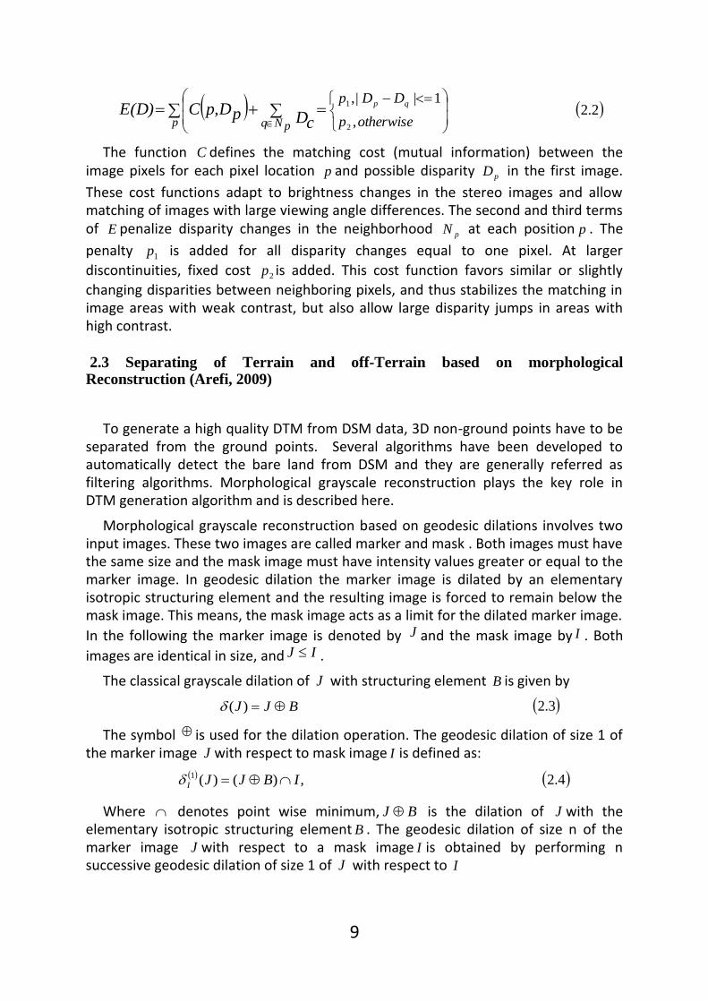
The function C defines the matching cost (mutual information) between the image pixels for each pixel location p and possible disparity pD in the first image.

These cost functions adapt to brightness changes in the stereo images and allow matching of images with large viewing angle differences. The second and third terms of E penalize disparity changes in the neighborhood pN at each position p . The

penalty 1p is added for all disparity changes equal to one pixel. At larger

discontinuities, fixed cost 2p is added. This cost function favors similar or slightly

changing disparities between neighboring pixels, and thus stabilizes the matching in image areas with weak contrast, but also allow large disparity jumps in areas with high contrast.

2.3 Separating of Terrain and off-Terrain based on morphological Reconstruction (Arefi, 2009)

To generate a high quality DTM from DSM data, 3D non-ground points have to be separated from the ground points. Several algorithms have been developed to automatically detect the bare land from DSM and they are generally referred as filtering algorithms. Morphological grayscale reconstruction plays the key role in DTM generation algorithm and is described here.

Morphological grayscale reconstruction based on geodesic dilations involves two input images. These two images are called marker and mask . Both images must have the same size and the mask image must have intensity values greater or equal to the marker image. In geodesic dilation the marker image is dilated by an elementary isotropic structuring element and the resulting image is forced to remain below the mask image. This means, the mask image acts as a limit for the dilated marker image.

In the following the marker image is denoted by J and the mask image by I . Both

images are identical in size, and IJ .

The classical grayscale dilation of J with structuring element B is given by

BJJ )( 3.2

The symbol is used for the dilation operation. The geodesic dilation of size 1 of the marker image J with respect to mask image I is defined as:

,)()(1 IBJJI 4.2

Where denotes point wise minimum, BJ is the dilation of J with the elementary isotropic structuring element B . The geodesic dilation of size n of the marker image J with respect to a mask image I is obtained by performing n successive geodesic dilation of size 1 of J with respect to I

11

n

III

n

I JJJ )1()1()1()( ....)()( 5.2

Equation 2.5 defines the morphological reconstruction by geodesic dilation of the mask I from the marker J . The desired reconstruction is achieved by carrying out geodesic dilations until stability is reached (Vincent, 1993). In other words, morphological reconstruction can be thought of conceptually as repeated dilations of the marker image until the contour lines of the marker image fits under the mask image. Each successive dilation operation is forced to lie underneath the mask. When further dilations do not change the marker image any more, the processing is finished. The final dilation creates the reconstructed image. Figure 2.2 illustrates the morphological reconstruction by means of geodesic dilations of D1 signal I from a marker signal .hIJ

By subtracting the reconstructed image from the mask image the normalized DSM (nDSM) is obtained.

A first classification of terrain and off-terrain points is carried out by binarising the nDSM. Any point (in the nDSM) above zero is collected as an off-terrain point.

Figure 2.2 Morphological reconstruction by

geodesic dilation of D1 mask signal I from a

marker signal .hIJ . (From H.Arefi 2009)

11

3 DTM quality assessment

With the upcoming of new technologies for the acquisition of terrain data and new developments in the area of digital photogrammetry due to automatic image matching techniques and revolution of laser scanning for capture of topographic data the question of quality" how accurate is DTM?" has to be studied new.

In this manner several methods have been already proposed based on statistical methods or visual interpretation.

In the first section of this chapter several enhanced visual techniques for quality assessment are described. Second part is dedicated to measures for accuracy assessment of DTMs based on robust statistical methods.

3.1 Visual methods for DTM quality assessment

Visual methods can be very important for the evaluation of DTMs and can balance some weakness of statistical methods.

The usage of visual methods depends on the expertise and experience of the operator. Visual methods actually offer the first assessments of DTMs ( Prodobnikar, 2009). In the following some of the visualization techniques and corresponding performance for DTM quality are introduced.

(1) 2D raster rendering

One of the most common ways to display DTMs is to associate each elevation with a color band. The resulting image broadly indicates topography and might also impliy any blunder in the elevation models.(Figure 3.1). The only form of data error likely to be detected using this method is that of blunders which significantly are observed by localized deviations in elevation value.

(2) Bi-polar difference maps

Two elevation surfaces are available, one of which is known to be of higher accuracy than the other, a difference map is produced using simple map algebra.

(3) Pseudo-3D projection: it represents the surface topography by two sets of orthogonal lines that follow the shape of the surface (Figure 3.2). In this method a 3

dimensional viewing location in polar coordinates r,, and surface location of zyx ,, are given. Next the screen coordinates YX , using homogeneous matrices can be calculated based on these data as follows:

100

0cossin0

0sinsinsincoscos

0cossincoscossin

1,,,,,

r

zyxzyx eee

1.3

where eee zyx ,, are the 3-dimensional viewing coordinates.

12

e

e

e

e

z

ydY

z

xdX , Where d is a scaling coefficient that represents the distance

from viewpoint to screen.

This method produces a realistic rendering of the elevation model surface and does not suffer from the quantization of elevation into bands. 3D projections offer more intuitive views than 2D rendering, but changes in parameters like viewing distance, field of view and vertical exaggeration can be misleading.

(4) Shaded relief maps: Generally processes that work based on local neighbors are more likely sensitive to the types of internal errors. One such process is calculating local shaded relief (Yeoli, 1967; Brassel, 1974). Principally, gray values depend on slope and aspect which are both calculated from the DEM. Then the illumination model determines the gray value of each pixel by calculating the cosine of the angle between the surface normal and the light vector (Foley et al., 1990)

This local operator provides a more discriminating way of looking at local variation. The disadvantage of this method is a danger of only selectivity highlighting parts of the elevation model in specific direction. For example considering only southeast and northeast slopes only (Wood and Fisher, 1993)

Figure 3.1: solid colored 2D raster s

are built with assigning elevation

classes to different colors

Figure 3.2: pseudo 3D projection of the same

area for figure 3.1. They represent the model

as 3D projection of intersecting orthogonal

lines

Figure 3.3: a shaded relief map for

the same area as preceding figures.

Clearly local topographic variation is

intuitive.

13

3.2 Accuracy measurement using robust statistical methods

Many of the statistical procedures assume that data are normally distributed. Unfortunately, when there are outliers in data, classical statistical methods often have very poor performance and large deviations from the normal distribution can cause problems (Heohle and Heohle, 2009).

As a simple example, let us consider n independent measurements of the same quantity, the question arises which value should be taken as the best estimate of the unknown true value. This question is answered if the error distribution is known and the arithmetic mean is accepted as a good estimator for unknown true value as long as normal distribution is considered as the distribution of error (Huber, 1972).

However empirical investigations show that the distribution of errors are slightly but clearly longer tailed because of this fact that real data normally contain outliers and their fraction is typically between 1 and 10 percent (Hampel et al, 1986). Therefore considering of outliers is crucial since they can play havoc with standard statistical methods.

Robust statistical measurements provide an alternative approach to classical statistical methods. The motivation is to produce estimators which are nonparametric and independent of error distribution (free distribution).

This chapter is organized in 2 sections; first section outlines statistical test and visual statistical methods as a component of good data analysis for investigating normality. In the second chapter robust accuracy measures suited for non normal error distributions are portrayed

3.2.1 Graphical Methods for test of normality

1. Histogram: The distribution of errors can be visualized by a histogram of the sampled errors, where the number of errors (frequency) within certain predefined interval is plotted and it is an estimate of the probability distribution of a continuous variable. Such a histogram gives a first impression of the normality of the error distribution. A better diagnostic to check the normality of error distribution is relied on two significant characteristics of histogram, namely skewness and kurtosis

Skewness is referred to asymmetry of the distribution. A distribution with an asymmetric tail extending out to the right is referred to as positively skewed or skewed to the right, while a distribution with an asymmetric tail extending out to the left is referred to as negatively skewed or skewed to the left. Skewness can range from minus infinity to positive infinity.

Figure 3.4: These figures depict the concept

of skwness in error histogram. Above figure

indicates that probability distribution has

fewer right values and longer right

tai(positive skewness), while figure below

shows a longer left tail, (negative skewness).

14

Kurtosis is introduced as a measure of how flat is the top of a symmetric distribution when compared to a normal distribution of the same variance (Pearson, 1905). It is actually more influenced by scores in the tails of the distribution than scores in the center of a distribution (De Carlo, 1967). Distribution with the positive kurtosis is fat in the tails. In contrast negative kurtosis depicts that distribution of errors is thin in the tails.

2. quantile-quantile plot: A better diagnostic plot for checking a deviation from the normal distribution is the so-called quantile-quantile(Q-Q)plot.

The Q-Q plot provides a more precise graphical test of whether a set of data could have come from a particular distribution. The data points,

d Tnddd ,..., 21 2.3

are first sorted in numerical order from smallest to largest into a vector y, which is plotted versus

)/)5.0((1 niFxi ),...,2,1( ni 3.3

Where )(xF is cumulative distribution function ( CDF ) of the distribution against which we wish to compare our observations.

If we are testing to see if the elements of d could have come from the normal distribution, then )(xF is the CDF for the standard normal distribution

dzexF

xz

N

2

2

1

2

1)(

4.3

If the element of d is normally distributed, the points ),( ii xy will follow a straight

line.

Figure 3.5: these figures describe

the notion of kurtosis. The

distribution of errors on the right

histogram has higher kurtosis than

the left one. It is more peaked at

the center, and it is has fatter tails.

Figure3.3: the Q-Q plot for a sample

dataset. A strong deviation from a straight

line is obvious which indicates the

distribution of dataset is not normal.

15

3.2.2 Statistical Tests for Normality

Many procedures for testing the normality of data samples have been posed in the literature. Considering only tests with composite null hypothesis, the goodness-of-fit statistic tests for normality can be grouped into four categories. The first one consists of measuring the distance between the theoretical distance function and the empirical distribution function. The second class of statistics is derived by skewness and kurtosis. The third family is based on generalization of the classical Pearson's 2 .

The last class relies on regression tools (D'Agostino and Stephens, 1986; Thode, 2002). In this study Chi-Square Goodness-of-fit in third category is portrayed to compare the observed sample distribution with the expected probability distribution function.

3.2.2.1 Chi-Square Goodness-of-Fit

This test establishes whether or not an observed frequency distribution differs from a theoretical distribution. A chi square test is applicable as long as sample data consists of these assumptions:

1. Random samples: A random sampling of the data from a population is provided.

2. Sample size: A sample with a sufficiently large size is assumed.

3. Independence: the observations are assumed to be independent of each other.

The chi square test is defined for hypothesis 0H , namely data follow a specific distribution and 1H , which means data don't follow a specific distribution. For the chi-square goodness-of-fit computation, the data are divided into k bins and the test statistic is defined as:

i

i

k

i i

E

EO 2

12)(

5.3

Where iO is the observed frequency for bin i and iE is the expected frequency for

bin i. The expected frequency is calculated by:

iui YFYFNE 6.3

Where F is the cumulative Distribution Function for the distribution is being tested,

uY is upper limit for class i, lY is the lower limit for class I and N is sample size.

The test statistics follows approximately, a chi- square distribution with ck degree of freedom where k is the number of non-empty bins and c is the estimated parameters for the distribution plus 1.

Therefore the hypothesis that data are from a population with the specific distribution is rejected if:

2

),(

2

ck 7.3

16

3.2.3 Robust accuracy measures suited for non-normal error distributions.

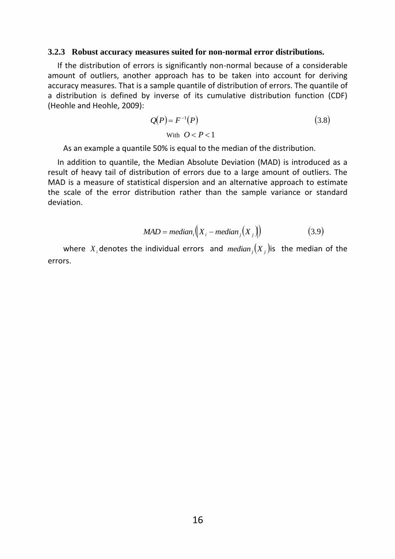
If the distribution of errors is significantly non-normal because of a considerable amount of outliers, another approach has to be taken into account for deriving accuracy measures. That is a sample quantile of distribution of errors. The quantile of a distribution is defined by inverse of its cumulative distribution function (CDF) (Heohle and Heohle, 2009):

PFPQ 1 8.3

With 1 PO

As an example a quantile 50% is equal to the median of the distribution.

In addition to quantile, the Median Absolute Deviation (MAD) is introduced as a result of heavy tail of distribution of errors due to a large amount of outliers. The MAD is a measure of statistical dispersion and an alternative approach to estimate the scale of the error distribution rather than the sample variance or standard deviation.

jjii XmedianXmedianMAD

9.3

where iX denotes the individual errors and jj Xmedian is the median of the

errors.

17

4 Evaluation of filtering efficiency as a part of DTM generation algorithm.

As mentioned before several methods for generation of Digital Surface Model have been proposed and executed. However, it should be noted that DSMs include many 3D objects such as buildings, trees and cars, therefore classification and extraction of bare earth is needed for DTM generation. To evaluate the accuracy of produced DTM it is also vital to assess the performance of filtering algorithm for separating ground and non-ground pixels.

As stated in chapter 2, the filtering algorithm implemented in the DTM generation procedure is based on mathematical morphology; corresponding techniques were discussed. This chapter is dedicated to determine the performance of this filtering algorithm and make a comparison with some others well known filtering algorithms based on presented datasets in ISPRS-commission III, working group III/3 "3D reconstruction from Airborne Laser Scanner and InSAR Data".

This chapter comprises in two sections. In the first section datasets and corresponding areas are presented and some terms relevant to this work are described. In the second part a brief review of the algorithm compared to the DLR algorithm is given first. Afterwards the filter data is compared to the reference that was generated by manual filtering of the DSM data and the output of the filter algorithm is compared against reference data. For evaluation of Type I and type 2 errors for feature in landscape, the cross-matrices are produced and the size of the error between the reference and filtered DSM is computed and analysis.

4.1 Test data.

To determine the filter difficulties pertaining to outliers, object complexity, attached objects, vegetation and discontinuities in the bare Earth, fifteen samples were extracted from eight datasets .These test data which were provided for this assessment are LIDAR dataset with resolution of 1-1.5 meter point spacing and are acquired from Vaihingen/Enz test field and Stuttgart city center. These areas are comprised of diverse feature content such as open fields, vegetation, buildings, roads, railroads, rivers, bridges, power lines, water surfaces. The properties of these selected sites are summarized in table 4.1.

Site Special features

1 Steep slopes, mix of vegetation and building in hill sides

2 Large building, irregularly shaped buildings, road with bridge and small tunnel

3 Density packed building with vegetation between them, open space with mixture of low and high features

4 Railway station with trains

5 Steep slopes with vegetation quarry, vegetation on river bank

6 Large building, road with embankment

7 Bridge, Underpass, road with embankments.

8 High bridge, break-line, vegetation on river bank

Table 4.1 properties of selected sites.

18

Figure4.1 Outlier in LIDAR dataset

Figure 4.3 a sample of complex object

Before proceeding to examine of filter algorithm it should be cited here that input data for the filtering algorithm have to be in a grid format. Therefore regularly spaced elevation grid points are founded by nearest neighbor interpolation of raw 3D laser points. The nearest neighbor interpolation is used to avoid smoothing over discontinuities given in the raw data.

For more clarification, some of the terms used for description of properties of selected area and are applied in continuation of this chapter defined as follow:

(1) Landscape: it consists of bare earth and any other features such as buildings, trees, power lines, etc.

(2) Detached objects: objects that stand on the bare Earth vertically on all sides such as trees or buildings.

(3) Attached objects: they pose on the bare earth vertically on some sides but not all e.g., bridges, ramps etc.

(4) Outliers: the term of outliers is addressed

to such points that normally are not part of

landscape.

(5) Large objects: herein if the size of objects goes beyond the test neighborhood, such objects are large objects.

(6) Small objects: the objects with 10 LIDAR data points or less are classified as small objects. For instance cars are prominent example of such objects.

(7) Very low objects- the objects that are very close to the bare earth are classified as very low objects and generally are difficult to detect in filtering algorithms.

(8) Complex objects: this term is assigned to features with complexity in shape, and configuration.

(9) Disconnected terrain- the reason for occurrence of this situation is enclosing bare earth with surrounded objects.

(10) Very low vegetables: like very low objects which are very close to the bare Earth.

Figure 4.2 Large, Small and Low objects

19

(11) Preservation (steep slopes)- these situations occur when the bare earth is piecewise continuous and produce misleading for those filtering algorithms that work with assumption of the objects are appears as discontinuities in landscape.

4.2 Assessment of filtering performance

As stated in beginning of the chapter, for performance evaluation of filtering algorithm, cross matrices are generated for different areas and then these matrices are used to evaluate type 1 (classify bare Earth points as object points) and type 2 errors (classify object point as bare earth pints) for corresponding areas. Before proceeding with this section a brief overview and description of compared algorithms with DLR algorithm is summarized in table 4.2

Developer(s) Filter description

M. Elmqvist-FOI(Swedish Defense Research institute), Sweden

Active Contour- Elmqvist(2001)

G. Sohn- University College London(UCL) Regularization method- Sohn(2002)

M. Roggero- Politecnico di Torino Modified slope based filter- Roggero (2001)

M.Brovelli- Politecnico di Milano Spline interpolation- Brovelli(2002)

R. Wack, A.Wimmer- Joanneum Research institute of Digital image processing

Hierarchical Modified Block Minimum- wack(2002)

P. Axelsson – DIGPRO Progressive TIN densification- Axelsson(1999-2000)

G. Sithole, G.Vosselman- TU Delf Modified Slope Based filter- wosselman(2000), Sithole(2001)

N. Pfeifer, C. Briese- TU Vienna Hierarchic robust interpolation – Pfeifer et. al.(1998), Briese et al.(2001)

Figure 4.4 Steep slopes which courses that

discontinuities in bare Earth are lost.

Table 4.2: structures and corresponding developer of different filtering algorithms (from

Sithole,2003).

21

Unused

Refe

ren

ce Bare Earth

Object

a b

c d

Participant

Filtered

Bare Earth(BE) Object

a+b

c+d

j

Ratio

dcba

baf

ca db dcbae

c

bK

dcba

dcg

ccba

cah

dcba

dbi

Std Dev

Totall

Type 2

Type 1

Min

p

q r s t

%

l m n

Max Mean

ba

b

dc

c

e

cb

To calculate the type 1 and type 2 errors, process of generating of cross matrices is presented as follow:

Table 4.3 Cross-matrices

The parameters that are indicated in above table are portrayed follow as:

a, is the number of Bare Earth points that have been correctly identified as Bare Earth.

b, is the number of Bare Earth points that have been incorrectly identified as objects

c, is the number of object points that have been incorrectly identified as Bare Earth.

d, is the number of object points that have been correctly identified as object.

e, is the total number of points which are tested.

a+b, c+d are total number of Bare Earth and object points in the reference data respectively.

a+c, b+d, are the total number of Bare Earth and object points in filter data respectively.

f,g are the proportions of Bare Earth and object points in the reference data in relation to the tested data respectively.

h, i are the proportions of Bare Earth and object points in filter data in relation to the tested data respectively.

K, ratio of number of type 1 and type 2 errors.

To present the type 1 and type 2 another table based on the values of cross-matrices is needed which is shown as follow:

Table 4.4 this table show s the error type 1 and 2 and corresponding distribution of them

21

UNUSED j

38010

Filtered

Bared Earth Object

12906

PARTICIPANT

21786

16224

0.573165

0.426835

Bare Earth

Object

Refe

rence

Ratio 2.026823

15061 6725

3318

18379 19631

0.48353065 0.51646935

Table 4.5: Cross –matrix for sample points 1-1

Table 4.6 Corresponding error type 1 and 2 for sample points 1-1

% Min% Max% Mean% Std Dev

0.126

26.42199

Type2

Total

30.86845 1.2 34.2 15.01

20.45118 1 49.6 16.6

TypeI1 0.112

%, is the percentage of type 1, type 2, or total error

L, m is the magnitude of the minimum and maximum type 1 error respectively

N, is the mean of the type 1 errors

P, is the standard deviation of the type 1 errors

q, r, is the magnitude of the minimum and maximum type 2 error respectively

s, is the mean of the type 2 errors

t, is the standard deviation of the type 2 errors

Moreover for fifteen samples from 8 sites which have been already mention in preceding section their corresponding cross-matrices are created and relevant errors type 1 and type 2 are computed.

Site1- the spesific properties of this area are steep slopes, mix of vegetation and building in hillsides. Two sorts of sample points are extracted from this area.

(1-1) Sample points 1 with properties of vegetation and building on sleep slopes. Corresponding cross matrices and error types are shown as follow:

Figure 4.5: 3D visualization of site 1.

22

UNUSED j

52119

Ratio 9.479419

Refe

rence

Bare Earth 18861 7830 266910.512117

Object 826

19687 32432

0.377731729 0.622268271

2460225428

PARTICIPANT

Filtered

Bared Earth Object

0.487883


Total0.166081

Type20.032484

1 49.6 16.6 0.126

TypeI10.293357

1.2 34.2 15.01 0.112

(1-2) Sample points 2 with property of small object. Corresponding cross matrices and error types are shown as follow:

Elmqvist

SohnAxelsson

Pfeifer

Brovelli

Roggero

wackSithol

eArefi

type1 error 33.63 26.56 15.96 28.26 62 33.16 39.12 37.69 30.86

Total errors 22.4 20.49 10.76 17.35 36.96 20.8 24.02 23.25 26.42

0

10

20

30

40

50

60

70p

erc

en

tage

Figure 4.6: Comparison of error type 1 for DLR algorithm (Arefi) respect to other

different algorithm for sample points 1-1


Table 4.8: Corresponding error type 1 and 2 for sample points 1-2

23

UNUSED j

12960

Ratio 3.408511

Refe

rence

Bare Earth 8483 1602 100850.778164

Object 470

8953 4007

0.690817901 0.309182099

2405 2875

PARTICIPANT

Filtered

Bared Earth Object

0.221836


Total15.98765

Type216.34783

1 49.6 16.6 0.126

TypeI115.88498

1.2 34.2 15.01 0.112

Site 2 – this area is composed of features with properties of large building, irregularly shaped buildings, road with bridge and small tunnel. Four different types of sample datasets with disparate characteristics are identified from this area as follow:

(2-1) Sample points 1 with property of Narrow building. Corresponding cross matrices and error types are shown as

follow:






Elmqvist

SohnAxelsson

Pfeifer

Brovelli

Roggero

wackSithol

eArefi

type1 error 12.36 8.87 4.89 7.29 29.63 11.92 11.94 19.19 29.3

Total errors 8.18 8.39 3.25 4.5 16.28 6.61 6.61 10.21 16.6

0

5

10

15

20

25

30

35p

erc

en

tage

24

UNUSED j

32706

Ratio 1.172823

Refe

rence

Bare Earth 19837 2667 225040.688069

Object 2274

22111 10595

0.676053324 0.323946676

7928 10202

PARTICIPANT

Filtered

Bared Earth Object

0.311931


Total15.10732

Type222.28975

1 49.6 16.6 0.126

TypeI111.85123

1.2 34.2 15.01 0.112

(2-2) Sample points 2 with features of bridge (south west)/gang way (North East). Corresponding cross matrices and error types are shown as follow:

Elmqvist

SohnAxelsson

Pfeifer

Brovelli

Roggero

wackSithol

eArefi

type1 error 25.91 8.38 0.046 2.81 11.35 12.46 5.15 9.64 15.8

Total errors 8.53 8.8 4.25 2.57 9.3 9.84 4.55 7.76 15.98

0

5

10

15

20

25

30p

erc

en

tage





25

UNUSED j

25095

0.473082

0.492488544 Ratio 1.382862

Refe

rence

Bare Earth 11464 1759 132230.526918

Object 127210600

11872

12736 12359

0.507511456

PARTICIPANT

Filtered

Bared Earth Object


Total12.0781

Type210.71429

1 49.6 16.6 0.126

TypeI113.30258

1.2 34.2 15.01 0.112

(2-3) Sample points 3 with features of large building, complex building and disconnected terrain. Corresponding cross matrices and error types are shown as follow:

Elmqvist

SohnAxelsson

Pfeifer

Brovelli

Roggero

wackSitho

leArefi

type1 error 20.55 5.68 2.68 8.25 31.19 33.43 9.73 29.29 11.85

Total errors 8.93 7.54 3.63 6.71 22.28 23.78 7.51 20.86 15.1

0.00

5.00

10.00

15.00

20.00

25.00

30.00

35.00

40.00

pe

rce

nta

ge

Figure 4.10: Comparison of error type 1 for DLR algorithm (Arefi) respect to

other different algorithm for sample points 2-2



26

UNUSED j

7492

Ratio 1.916473

Refe

rence

Bare Earth 4608 826 54340.725307

Object 431

5039 2453

0.67258409 0.32741591

16272058

PARTICIPANT

Filtered

Bared Earth Object

0.274693

(2-4) Sample points 4 with features of ramp. Corresponding cross matrices and error types are shown as follow:

Elmqvist

SohnAxelsson

Pfeifer

Brovelli

Roggero

wackSithol

eArefi

type1 error 18.74 7.25 3.69 12.08 50.25 41.88 18.4 40.92 13.3

Total errors 12.28 9.84 4 8.22 27.8 23.2 10.97 22.71 12.07

0

10

20

30

40

50

60p

erc

en

tage


Total16.7779

Type220.94266

1 49.6 16.6 0.126

TypeI115.20059

1.2 34.2 15.01 0.112





27

UNUSED j

28862

Ratio 16.06061

Refe

rence

Bare Earth 10786 4770 155560.538979

Object 297

11083 17779

0.383999723 0.616000277

1300913306

PARTICIPANT

Filtered

Bared Earth Object

0.461021

Site 3- this region comprises of areas with density packed building and vegetation between them and open space with mixture of low and high features. Therefore the sample datasets possess the characteristics of disconnected terrain and low objects. Corresponding cross-matrices and error types are presented as follow:

Elmqvist

SohnAxelsson

Pfeifer

Brovelli

Roggero

wackSithol

eArefi

type1 error 31.8 13.17 3.38 8.54 47.63 30.43 14.41 32.79 15.2

Total errors 13.83 13.33 4.42 8.64 36.06 23.25 11.53 25.28 16.77

0

10

20

30

40

50

60

pe

rce

nta

ge





28


Total17.55596

Type22.232076

1 49.6 16.6 0.126

TypeI130.66341

1.2 34.2 15.01 0.112

Elmqvist

SohnAxelsson

Pfeifer

Brovelli

Roggero

wackSithol

eArefi

type1 error 8.47 4.81 7.91 1.6 21.75 3.03 3.15 4.85 30.66

Total errors 5.34 6.39 4.78 1.8 12.92 2.14 2.21 3.15 17.55

0

5

10

15

20

25

30

35

pe

rce

nta

ge




29

UNUSED j

11231

Ratio 0.23622

Refe

rence

Bare Earth 4942 660 56020.498798

Object 2794

7736 3495

0.688807764 0.311192236

28355629

PARTICIPANT

Filtered

Bared Earth Object

0.501202


Total30.75416

Type249.63581

1 49.6 16.6 0.126

TypeI111.78151

1.2 34.2 15.01 0.112

Site4- This area consists of Railway station with trains and two different sample datasets with following characteristics are taken out.

(4-1) Sample points 1 with clump of low points (multi path errors). Corresponding cross matrices and error types are shown as follow:

Figure 4.15: 3D visualization of site 4



31

UNUSED j

42470

0.707017

0.799387803 Ratio 12.78078

Refe

rence

Bare Earth 8187 4256 124430.292983

Object 333 29694 30027

8520 33950

0.200612197

PARTICIPANT

Filtered

Bared Earth Object


Total10.80527

Type21.109002

1 49.6 16.6 0.126

TypeI134.20397

1.2 34.2 15.01 0.112

(4-2) Sample points 2 with elongated objects, low objects and high frequency variation in the landscape. Corresponding cross matrices and error types are shown as follow:

Elmqvist

SohnAxelsson

Pfeifer

Brovelli

Roggero

wackSithol

eArefi

type1 error 14.42 19.25 25.81 19.85 32.41 21.55 17.63 47.13 11.7

Total errors 8.76 11.27 13.91 10.75 17.03 12.21 9.01 23.67 30.75

0

5

10

15

20

25

30

35

40

45

50

pe

rce

nta

ge





31

UNUSED j

17845

Ratio 0.707853

Refe

rence

Bare Earth 13274 676 139500.781732

Object 955

14229 3616

0.797366209 0.202633791

29403895

PARTICIPANT

Filtered

Bared Earth Object

0.218268


Total9.139815

Type224.51861

1 49.6 16.6 0.126

TypeI14.845878

1.2 34.2 15.01 0.112

Site 5- Steep slopes with vegetation quarry and vegetation on river bank are characteristics of this area. Based on these properties three different sorts of datasets are extracted.

(5-1) Sample points 1 from area with vegetation on slopes. Corresponding cross matrices and error types are shown as follow:

Elmqvist

SohnAxelsson

Pfeifer

Brovelli

Roggero

wackSithol

eArefi

type1 error 4.3 1.01 4.68 8.02 20.4 13.37 10.65 12.18 34.2

Total errors 3.68 1.78 1.62 2.64 6.38 4.3 3.54 3.58 10.8

0

5

10

15

20

25

30

35

40p

erc

en

tage





Table 4.23: Corresponding error type 1 and 2 for

sample points 5-1

32

UNUSED j

22474

Ratio 0.333333

Refe

rence

Bare Earth 19868 244 201120.894901

Object 732

20600 1874

0.916614755 0.083385245

16302362

PARTICIPANT

Filtered

Bared Earth Object

0.105099


Total4.342796

Type230.99069

1 49.6 16.6 0.126

TypeI11.213206

1.2 34.2 15.01 0.112

(5-2) these sample datasets are from areas with low vegetation, discontinuities and sharp regions. Corresponding cross matrices and error types are shown as follow:

Elmqvist

SohnAxelsson

Pfeifer

Brovelli

Roggero

wackSithol

eArefi

type1 error 49.34 10.33 0.13 4.21 28.23 1.9 14.03 7.03 4.8

Total errors 21.31 9.31 2.72 3.71 22.81 3.01 11.45 7.02 9.13

0

10

20

30

40

50

60p

erc

en

tage





33

UNUSED j

34378

12801389

PARTICIPANT

Filtered

Bared Earth Object

0.040404

32538 1840

0.946477398 0.053522602 Ratio 5.137615

Refe

rence

Bare Earth 32429 560 329890.959596

Object 109

(5-3) these sample datasets are from areas with discontinuities in the bare earth with low Vegetation, discontinuities and sharp regions. Corresponding cross matrices and error types relevant to such region are shown as follow:

Elmqvist

SohnAxelsson

Pfeifer

Brovelli

Roggero

wackSithol

eArefi

type1 error 85.05 12.34 1.78 21.27 50.43 9.8 26.49 30.41 1.21

Total errors 57.95 12.04 3.07 19.64 45.56 9.78 23.83 27.53 4.34

0

10

20

30

40

50

60

70

80

90p

erc

en

tage

Figure 4.20: Comparison of error type 1 for DLR algorithm (Arefi) respect to other different

algorithm for sample points 5-2



Total1.946012

Type27.847372

1 49.6 16.6 0.126

TypeI11.697536

1.2 34.2 15.01 0.112


34

UNUSED j

8608

Ratio 0.54386

Refe

rence

Bare Earth 3766 217 39830.462709

Object 399

4165 4443

0.48385223 0.51614777

42264625

PARTICIPANT

Filtered

Bared Earth Object

0.537291


Total7.156134

Type28.627027

1 49.6 16.6 0.126

TypeI15.448155

1.2 34.2 15.01 0.112

(5-4) these sample datasets are acquired from areas consist of low resolution buildings. Corresponding cross matrices and error types are shown as follow:

Elmqvist

SohnAxelsson

Pfeifer

Brovelli

Roggero

wackSitho

leArefi

type1 error 92.45 20.48 8.58 12.53 54.93 17.81 28.33 38.41 1.69

Total errors 48.45 20.19 8.91 12.6 52.81 17.29 27.24 37.03 1.94

0

10

20

30

40

50

60

70

80

90

100

pe

rce

nta

ge





35

UNUSED j

35060

Ratio 8.974843

Refe

rence

Bare Earth 32427 1427 338540.965602

Object 159

32586 2474

0.929435254 0.070564746

1047 1206

PARTICIPANT

Filtered

Bared Earth Object

0.034398

Site6- The predominant characteristic of this area is large buildings and roads with embankment. Based on these properties sample datasets are acquired from areas with discontinuities and sharp ridges.

Elmqvist

SohnAxelsson

Pfeifer

Brovelli

Roggero

wackSithol

eArefi

type1 error 27.91 6.72 1.25 10.66 49.54 1.01 15.93 12.38 5.44

Total errors 21.26 5.68 3.23 5.47 23.89 4.96 7.63 6.33 7.15

0

10

20

30

40

50

60

pe

rce

nta

ge





36


Total4.523674

Type213.18408

1 49.6 16.6 0.126

TypeI14.215159

1.2 34.2 15.01 0.112

Site7- This region includes bridge, Underpass, and road with embankments. Corresponding cross matrices and error types for sample datasets acquired from this region are shown as follow:

Elmqvist

SohnAxelsson

Pfeifer

Brovelli

Roggero

wackSitho

leArefi

type1 error 91.28 2.96 1.94 7.15 22.45 19.64 13.94 22.39 4.21

Total errors 35.87 2.99 2.08 6.91 21.68 18.99 13.47 21.63 4.52

0

10

20

30

40

50

60

70

80

90

100

pe

rce

nta

ge






37

UNUSED j

15645

Ratio 6.280236

Refe

rence

Bare Earth 11746 2129 138750.886865

Object 339

12085 3560

0.772451262 0.227548738

1431 1770

PARTICIPANT

Filtered

Bared Earth Object

0.113135


Total15.77501

Type219.15254

1 49.6 16.6 0.126

TypeI115.34414

1.2 34.2 15.01 0.112

Elmqvist

SohnAxelsson

Pfeifer

Brovelli

Roggero

wackSithol

eArefi

type1 error 75.19 1.26 0.14 9.78 39.41 5.41 18.88 24.57 1.53

Total errors 34.22 2.2 1.63 8.85 34.98 5.11 16.97 21.83 15.77

0

10

20

30

40

50

60

70

80

pe

rce

nta

ge





38

Interpretation of results:

According to above results the performance of the algorithm is interpreted based on the properties of the areas under study, namely steep slopes, discontinuities, complex scene, vegetation on slopes, low bare earth count and bridges. A significant remark regarding to the DLR filtering approach (Arefi,2009) needs to be considered about the 3D objects connected to the image borders. According to this filtering approach that is based on the hierarchical filtering of the non-ground pixels, only the objects which are entirely located inside the image will be filtered. Therefore, if any parts of 3D objects such as buildings are connected to the image border they will be filtered by this approach. Accordingly, to process on a special area it is suggested by the author that a larger area be considered for filtering to be sure all the 3D objects on desired region are filtered. This limitation increases the rate of errors comparing to the other algorithms.

Steep slopes- sample datasets 1-1, 5-1 belongs to such areas with property of steep slope. As might be seen there is significant bias towards type 1 errors and less towards type 2 errors, namely 30.86 and 20.45 % respectively for sample 1-1. In contrast for data samples 5-1 and 5-2 the error type 1 declines considerably to 4.84 and 1.24 % respectively and this is the least type 1 error in comparison with other mentioned algorithms for datasets 5-1. This means that filtering algorithm operates quite well for vegetation areas even though they lie on the steep slope but there is still problem for buildings areas.

Discontinuities – discontinuity is presented in datasets 2-2, 2-3, and 5-3. In according to corresponding type 1 errors for these datasets, namely 11.85, 13.30 and 1.69, general performance of the filtering algorithm for such areas is well especially for vegetation area. It should be noted that the performance of the filtering algorithm for sample points 5-3 acquired to examine the behavior of filter algorithms for discontinuity preservation is excellent in comparison with other filtering algorithms.

Complex scene- complex senses are presented in sample datasets 1-1, and 2-3 with corresponding errors type 1, 30.86, 11.85, and 13.30 respectively. As might be seen the performance of filtering algorithm for complex buildings lied on the steep slope areas( with error type30.86) is worse for those areas(datasets 23) with complex structures building located in nearly flat area.

Bridges and ramps - approximately all filters are blind to distinguish between objects that stand clear of the bare earth and those that are attached to the bare earth (Sithole,2003), and thus DLR filter algorithm is not exempt from this fact. By considering datasets 2-1, 2-4 and 7-1 pertaining to areas with bridge and ramp, and their respective errors 15.88, 15.20 and 15.34 corresponding of this error for other algorithms, it is concluded that the performance of filter is well and base on the visual result more and less all the bridge and ramp removed . However as already mentioned there are some problems in beginning and end of bridges.

Vegetation on slopes- datasets 5-1 and 5-2 are examples of vegetation on slopes.

39

As can be seen the functionality of filter algorithm for these areas based on respective 4.84 and 9.13 errors type1, is quite well, in particular identification of filter for low vegetables with only 1.21 % error type 1 and 4.34 % total errors in comparison with other errors is outstanding. However, the accuracy of filter for vegetation on slope is a little less than flat area.

Low bare earth point count- In general it is crucial there be enough sample points for bare earth for identification of this area by filter algorithm. This circumstance occurs in datasets 4-2 belong to railway station. According to type 1 error (34%) for this data the efficiency of filter algorithm in this situation is poor. Therefore, adequate number of points acquired from bare earth is crucial for efficiency of filter algorithm.

Conclusion - initially it has to be emphasized that general performance of filter algorithm is quite well in particular for vegetation areas. However, some difficulties in filtering were observed in complex landscape especially those that located on steep slopes. In general, from type 1 and 2 errors, for areas corresponding to sample points 12,31 and 4-2 with significant error type 1 the filter algorithm focuses on minimizing type 2 errors. This means that functionality of filtering algorithm is based on to remove the objects as many as possible even though if the valid terrain is also removed. The suppression of the effect might be appeared by choosing appropriate filter parameters for such areas. Finally, it should be mentioned that all comparisons are made without considering the limitation of the DLR filtering about the 3D objects connected to image borders. This has particularly a negative effect on the filtering of the sites 1, 2, 3, and 4 where many large buildings are connected to the image border.

41

5 DTM Accuracy Assessments

As it was already mentioned in preceding chapters, nowadays several techniques are available for generation of DSMs and corresponding DTMs that they represent the bare earth at some level of details and in fact demands on DTMs are still growing continuously. While new techniques such as LIDAR are available for almost instant DSM generation, the use of stereoscopic high-resolution satellite imagery (HRSI), coupled with image matching, affords cost-effective measurement of surface topography over large coverage area(Poon et al.,2005).However all these techniques imply the risk of error and ill determined areas. The objective of this chapter is to identify type and magnitude of errors, contribute in DTMs. It should be stressed here that as already cited DTM generation algorithm which is used in this study is based on semiglobal matching technique to produce the DSM and the rational of the filter used to separate the off terrain is pertaining to Mathematical morphology.

In general uncertainty in DTMs originates from two sources: 1) Gross, Systematic and random errors in lattice points, and 2) accuracy loss due to lattice representation of the terrain (Li et al., 2005). This chapter outlines the contribution and magnitude of errors in stage of data acquisition and processing data. This chapter is organized as follow: the first section introduces the stereo datasets which are open for benchmarking and the reference datasets. Second part of this chapter the contribution of random errors and corresponding magnitude is examined. In third part the cause of systematic errors and amount of such errors for different areas is evaluated. On the fourth part an algorithm based on robust statistical methods to determine the gross errors is proposed. The fifth chapter is dedicated to assess the amount of such errors for different sensors which are used for data acquisition. Through the entire chapter the fact of existing outlier is taken to account and robust statistical methods as an alternative for classical statistical methods are employed.

5.1 Study areas and data acquisition.

The test region in Catalonia, near Barcelona has been selected due to availability of several stereo satellite data and a high quality reference dataset provided by the Institute Cartografic de Catalunya(ICC). They consist of color orthoimages with a spatial resolution of 50 cm as well as an airborne laser scanning point cloud with approximately0.85 and 0.4 point per square meters for Lamola and Terrassa region respectively. The four ISPRS datasets are used for the test region. (ISPRS-Commission I, working group I /4, Benchmarking and quality analysis of DEM). The characteristics of these datasets and properties of selected test areas are described in table 1 and 2.

Figure 5.1 these images showing the two test areas, left image is Terrassa Region and right image

indicates Lamola area

41

The systematic errors of measured LIDAR points in according to (Husing et al., 1998) for flat, flat gross, hilly and hilly gross areas are 5-20, 20-200, 5-20 and 20-200 centimeter respectively.

Respective random errors for LIDAR data point for these areas are 10-20, 10-50, 20-200 and 20-200 centimeter.

Area Properties of selected test area

Height

Range

Mean Slope

degree Terrain

Description

Area

Size

Terrassa 281-311 12 City ,Industrial 5X5Km

La Mola 596-792 24.5

Mountainous

forest

5X5Km

Dataset Description of datasets

Image resolution(m) Generated DEM resolution(m)

Worldview -1 0.5 2.5

Table5.2 Properties of source datasets

Table 5.2 Terrains descriptive statistics

Figure 5.2: these images show the return density represented by each pixel area. Cells with

point densities falling within the .5 to 1 piont per square meter are colored green ,above this

range are colored blue and below are colored red corresponding to Lamola area(left) and

Terrassa area (right)

Figure 5.3 corresponding slope maps for Terrassa(left) and Lamola(right ) areas

Table 5.1 Properties of selected test area

42

The availability of very dense LIDAR data points gives the possibility of checking the generated DSM and thus In following generated DSMs by semiglobal stereo matching of World view-1 satellite images are compared with the first pulse laser points . More than 19 and 10million random LIDAR points for Lamola and Terrassa region respectively contribute to detect errors. it should be stated here that derived accuracy error for DSM is relative error respect to the accuracy of the LIDAR datasets. For evaluation of distribution errors, corresponding histograms and Q-Q plots for terrassa and lamola regions are shown in figure 1 and 2.

The both histograms show that the kurtosis of the errors distribution is positive, i.e. the distribution has a sharp peak around the mean and fatter and longer tails than normal distribution. Values for skewness of both error distributions indicate that deviation from the mean by outliers is going to be positive.

Alternatively to test of normality of distribution errors as stated in chapter 3, chi-square goodness-of-fit test is carried out. The computed chi values for corresponding areas as well as kurtosis and skewness are tabulated in table 3

Figure 5.4 Corresponding normalized histograms of h between Laser points and DSM for

Terrassa( Left) and Lamola(Right)

Figure 5.5 Corresponding Q-Q plots for Lamola(right) and Terrassa(Left) regions.

43

Figure 5.5 shows the Q-Q plots for corresponding regions. Both Q-Q plots diverge from straight line and it also can be seen there are more positive outliers than negative ones for Lamola region. In addition the bootstrap distribution of mean and median based on 50 bootstrap samples have been computed and shown in figure 5.6. It can be clearly seen that the distribution of mean in comparison to median is erratic as a result of outliers. According to the values of statistical parameters shown in table 5.33 and preceding discussion for presented graphs it can be concluded that there is an excessive amount of outliers in the observations. Furthermore robust statistical method which is resistant to outlier has to be applied.

Consequently median, 90 and 95 % sample quantiles of absolute errors and Median Absolute Deviation(MAD) as stated in chapter 3 are employed to estimate the accuracy of DSM respect to LIDAR datasets. And results are summarized in table 5.4 for corresponding areas.

Area

Statistical Measures

Skewness Kurtosis Computed chi-square

value

Chi square distribution value

α=%95,

Degree of freedom

Terrassa 00111 16.31 41877000 22.36 13

La Mola 6.50 74.61 183970000 42.56 29

Area Accuracy Measure

Mean Standard Deviation RMSE 50% quantile ∆h (m)

MAD ∆ (m) 68.3%quantile

|∆h| (m)

95%quantile

|∆h|(m)

Terrassa 0.349 4.23 4.25

0.116 2.43 2.16 9.72

La Mola -0.306 10.49 10.50

-1.59 8015 4.966 14.17

Table 5.3. Statistical measures to describe the distribution of observed errors for investigation areas.

Figure 5.6 This figure shows the bootstrap distribution of the mean (left) and median (left)

based on 50 bootstrap samples for each estimator.

Table 5.4 Accuracy measure of DSM generated by World views images respect to LIDAR

datasets

44

The plot in figure 5.7 shows the solid colored raster of difference between generated DSM by semiglobal matching and DSM derived by laser scanning. Grid surface for generated DSM by LIDAR points is created through bilinear interpolation. Additionally shaded relief map for DSM generated by semiglobal matching is also represented. It can be noted that outliers in shaded relief map are obvious. However, unlikely application of contour maps for outlier visualization in DSMs reduces due to surface discontinuity.

Figure 5.7 solid raster color error map for Terrassa area. As can be seen outliers are identified by a distinguish

color from their neighborhoods.

Figure 5.8 shaded relief map of generated DSM for Terrassa area by semiglobal matching. Outliers can be

detected directly without comparison to ground truth.

45

5.2 Random and systematic errors in generated DSM.

The word of random error indicates that they are inherently unpredictable and tend to have null arithmetic mean when the measurement is repeated several times and they have a normal distribution. Random errors are also referred to as white noise in statistics. For such errors, improvement of DSM quality is conducted by applying a low pass filtering (Li, 1990). A low-pass filter removes the high frequency

noise with the resulting output being a smoother grid. In this manner a 33 Gaussian low-pass filter is employed. With the Gaussian Low-pass filter, the weights fall-off with increased distance. Table 5.5 and 5.6 show the accuracy of DSM and amount of improvement percentage after filtering respectively.

33 Gaussian low pass filter

121

242

121

)1.5(

However, according to above results and achieved accuracy, necessity of applying filtering processes completely depends on magnitude of the random error occurring during the measurements. For example (Kubic and Roy, 1980) suggested 0.05% of flying height for photogrammetric measurement might be appropriate threshold.

Systematic errors are bias in the measurements caused by the situation where the mean of many separated measurements are different from the actual value of measured attributes. Systematic errors usually occur due to lack of adequate adjustment of instruments, and misalignment in georeferencing due to datum or processing errors. herein median of differences with o.112 and -1.586 meter for Terrassa and Lamola regions respectively are interpreted as systematic errors which are the values for systematic shift between the DSM and LIDAR datasets.




|∆h| (m)

95%quantile

|∆h|(m)

Terrassa 0.3492 4.161 4.176

0.1128 2.398 2.153 9.516

La Mola -0.306 10.266 10.271

-1.586 5.115 4.927 13.845

Area Accuracy improvement with random noise filtering(percentage)



|∆h| (m)

95%quantile

|∆h|(m)

Terrassa 0 1.6 1.7

2.8 1.3 0.3 1.9

La Mola 0 2.1 1.23 1.25 1.3 1.79 1.63

Table 5.5 Accuracy measure of DSM respect to LIDAR datasets after random noise filtering

Table 5.6 Accuracy improvement with random noise filtering

46

5.3 Outlier detection and removal in Digital Surface Model

Gross errors which are also called blunders, in fact can be any size in nature. Compared with random and systematic errors, they occur with small probability during measurements. In DSM generation Gross errors often occur in automatic image matching due to mismatching of image points.

It is obvious from Q-Q plot and also statistical measures from table 5.3, outliers exist and from table 5-4 this fact is deduced that they have a great influence on the estimated standard deviation. From this table for both areas 68.3% quantile and median absolute deviation are very close. However it should be noted that the 95% quintile for both regions are greater than two times the 68.3 % quantile due to fat tails of both distribution that clearly show the non-normality of errors.

To classify the outlier for accuracy measurements initially 3 times RMSE is considered and results are tabulated in table 5.7. with this threshold 1.5 and 2.5 percentage of data for Lamola and Terrassa regions are classified as outliers

As can be seen from table 5.7 the standard deviation and RMSE after removal of outliers are much lower as with outliers included. Additionally a improvement is observed in MAD and 68.3% quantle.

However , the condition of three times RMSE based on observed 95% quantiles for both areas are not completely fulfill our desire to achieve appropriate accuracy. Therefore in this project a new method to gain an appropriate threshold is proposed.

The methodology which is used here to detect the gross errors is based on the robust statistical measures and consists of four steps:




|∆h| (m)

95%quantile

|∆h|(m)

Terrassa 0.206 3.124 3.131 10100 2.114 2.113 7.54

La Mola -1.13 5.892

6.004 -1.636 4.02 4.81 12.522

Area Accuracy improvement with removing outliers by 3.RMSE(percentage)



|∆h| (m)

95%quantile

|∆h|(m)

Terrassa 69 33 25 14 21 7 26

La Mola -73 74

71 -3 24 3 11

Table 5.7 Accuracy measure of DSM. Herein outlier are classified by 3times of RMSE.

Table 5.8 Accuracy improvement with removing outliers by 3.RMSE (results are shown as

percentage).

47

(1) quantile .5 till quantile 1 are computed in sequence.

(2) Since linear least-squares estimators are badly affected by outliers, a robust regression estimator such as Least Median Square(LMS) is utilized to acquire regression parameters for computed quantiles and identify which quantiles are emerging as outlieres.

(3) Recording the index of first quantile which is recognized as an outlier. In this manner all quantiles are compared to corresponding estimated values by LMS. Corresponding quantile of first difference which is bigger than median absolute deviation is chosen. For example if quantile( .92) is recognized as outlier by least median square then.92 is saved as index of this quantile.

(4) Computing an appropriate threshold to remove the outliers. In this manner a certain confidence interval is proposed showing that observations (dh) lie within the interval based on Vysochanskij–Petunin theory[Vysochanskij,1980].

29

4

uxp (5.2)

For example based on this theory for any unimodal data sample, about 5% of the values are further than three standard deviations from the mean. However, as stated before, 3 times standard deviation doesn't fulfill our desire and cannot be an appropriate threshold. Moreover based on the sequence of the algorithm quantile 0.5 till 0.9 are computed. Figures 5.9 and 5.10 show that the values of corresponding quantile for both areas increase exponentially and relationship between the quantiles is not linear due to the fact of outliers. In these graphs corresponding Least

-2

0

2

4

6

8

10

12

14

16

18

Quantile Analysis for Terrassa Region

quantile 50% to 100% for |dh| in Lamola

LMS regression

Ordinary Least Square

Figure 5.9 this graph shows the amount of quanties from 0.5 to 0.99 of dh errors and

corresponding Least median square and ordinary least square for Terrassa area.

48

median square regression and ordinary least square line are plotted. It is obvious that the least square estimation is completely inefficient to estimate the true values of quantiles.

Conversely least median of square(LMS) regression as a robust estimator can resist the effect of nearly 50% of contamination in datasets (Rousseeuw,1984) and this mater can be noted clearly in these figures. In LMS the different approach is introduced in which the sum is replaced by median of the square residuals.

According to step 3, quantile 0.91 and 0.96 for terrassa and lamola are recognized respectively as outliers and their index 0.91 and 0.96 are saved. Finally based on (5.2) corresponding values of λ namely 2.22 and 3.3 for both areas are computed. Consequence respective 7.81 and 24.69 figures for Terrassa and Lamola are utilized as thresholds. Results of accuracy measure and corresponding percentage of improvement with considering the new value of thresholds for both areas are tabulated in table 5.7 and shown in figure 5.11 and 5.12

0

5

10

15

20

25

30

35

40

45

135791113151719212325272931333537394143454749

Quantile analysis for Lamola area

Quantile

LMS regression

Ordinary least square

Area

Accuracy Measure

Mean Standard

Deviation

RMSE 50%

quantile ∆h (m)

MAD ∆ (m)

Normalized

MAD

68.3%quantile

|∆h| (m)

95%quantile

|∆h|(m)

Terrassa 0.129 2.342 2.345 0.086 1.622 2.41 1.795 4.40

La Mola -1.21 5.57 5.70 -1.636 3.89 5.75 4.77 12.16

Figure 5.10 this graph shows the amount of quanties from 0.5 to 0.99 of dh errors and

corresponding Least median square and ordinary least square for Lamola area.

Table 5.9 Accuracy measure of DSM by applying new threshold computed by proposed method.

49

-4

-2

0

2

4

6

8

10

12

14

16

Accuracy improvement after applying appropriate threshold(Lamola)

Accurace measure before applying threshold

Accuracy measure after applying threshold

By applying the appropriate threshold for Terrassa and Lamola areas , 4.5 and 1.9 percentage of datasets are removed .

In the end the accuracy measures are computed by considering the thresholds based on proposed appropriate removal outliers method except that corresponding quantiles of first difference which are start to deviate from least median square line are chosen namely, quantiles of 81% and 80% and respective values of 1.52 and 1.49 are computed as threshold for Lamola and Terrassa areas correspondingly. However it has to be noted here Vysochanski theory functions for any λ>1.632. therefore λ=1.633 is chosen. Hence 5.79 and 12.12 are computed as appropriate thresholds for both areas and results are tabulated in table 5.7.

012345678910

Accuracy improvement after applying appropriate Threshold(Terrassa)

Accurace measure before applying threshold

Accuracy measure after applying threshold

Figure 5.11 Accuracy improvement after applying appropriate threshold for Terrassa area.

Figure 5.11 Accuracy improvement after applying appropriate threshold for Lamola area.

51

The standard deviation after removal of outliers for Terrassa area by applying 7.81 and cost of losing 4.5 percentage of dataset differ slightly from normalized MAD, namely 5.5 cm indicates that outliers removed very well. Additionally for Lamola area with value of 12.12 as threshold the cost of losing data is 7.37%. however as can be seen from table 5.7 standard deviation with normalized median and 68.3 quantile differs 47 and 5.6 cm respectively which is also very good indicator for successful outliers removal.

5.4 summary and discussion

In accuracy measures of DSM based on represented plots for histograms and Q_Q plots and corresponding skewness and kurtosis and also based on statistical chi-square goodness-of-fit results, the fact of existing outliers must be taken in account. In order to derive reliable value for systematic errors and standard deviation different approaches based on using all the data and also outlier removal according to three times RMSE threshold were used. Additionally a new methods based on quantile analysis to acquire appropriate threshold was proposed.

According to (Kraus, 2004) a formula that describes the height accuracy of topographic measurement by ALS is given in 5.3. Additionally quantification of systematic and random errors for LIDAR point is summarized in table 5.8.

Area

Accuracy Measure

Mean Standard

Deviation

RMSE 50%

quantile ∆h (m)

MAD ∆ (m)

Normalized

MAD

68.3%quantile

|∆h| (m)

95%quantile

|∆h|(m)

Terrassa 0.099 1.938 1.941 0.0782 1.401 2.178 1.63 4.382

La Mola -1.39 4.33 4.55 -1.668 3.246 4.80 4.386 9.482

Table 5.8 Quantification of systematic and random errors based on theoretical consideration.

(from Husing 1998)

5.10 Accuracy measure of DSM with λ=1.6.33 and respective thresholds 7.81 and 12.12 for Terrassa

and Lamola

51

tan50

6][

ncmH n Points per square meter )3.5(

For wooden area in (5.3) factor 0.25 has to be multiplied to n. consequently respective height accuracy of topographic measurements are 20.11 and 36 cm for Terrassa and Lamola regions. In addition the accuracy of source datasets indicated in table 5.8 has to be taken in account. Therefore computed accuracy for generated DSM respect to LASER data sets for Lamola region which is a hilly grass area is poor (RMSE 4.55 and NMAD 4.80) and also characteristics of such area influence the systematic error which is -1.39 and -1.69 for mean and 50% quantile .

However accuracy of DSM for Terrassa region comprised of regions with residential and hilly bared characteristics is much better namely, with RMSE 1.94 and NMAD 2.07m. In this area systematic error is small, around 0.8 centimeter.

52

6 conclusion and future recommendation

To measure the accuracy of DTMs and to improve it, the attributes of errors and their magnitudes have to be considered. Moreover we classified error characteristics as random, systematic and gross errors and evaluated significance of them.

it was concluded that general performance of filter algorithm is quite well in particular for vegetation areas. However, some difficulties in filtering were observed in complex landscape especially those that located on steep slopes.

Quality control of DSM by means of Visual inspection was introduced and concluded that such methods are able to detect and remove the outliers as many as possible.

The accuracy measures for generated DSM should not be influenced from outliers and non-normality of the error distribution. To avoid influence of outliers in error assessment robust statistical methods were proposed and based on them a method for gross error detection by analysis of quantile errors was proposed.

In the end according to final values obtained for two test areas it can be concluded that the performance of the DSM algorithm for mountainous wooden areas respect to the accuracy of LIDAR datasets is poor. Nevertheless in according to relative accuracy of urban area it can be concluded that DSM accuracy is able to follow the accuracy of LIDAR datasets.

Moreover in comparison to cost of using LIDAR system and according to this fact there is a possibility that some remained outliers removed by filter algorithm and consequently the accuracy of generated DTM is higher than DSM. Therefore by employing an appropriate interpolation method, generating DTM from high resolution satellite images in urban area can be an appropriate alternative for LIDAR systems.

53

Bibliography

Arefi, H (2009) From LIDAR point clouds to 3D building models. PhD thesis, Bundeswehr University Munich.

Aster R, Borchers B, Thurber C (2005) Parameter estimation and inverse problems. Academic press, Burlington:15-40

Axelsson P (2000) DEM generation from laser scanner data using TIN adaptive models. International Archive of photogrammetry and Remote Sensing, 33: 110-117

Axelsson P (1999) Processing of laser scanner data: algorithm and application. ISPRS journal of photogrammetry and Remote Sensing, 54: 138-147

Brovelli M (2002) Managing and processing LIDAR data within GRASS. In: proceeding of GRASS users Conference, Trento

D'Angelo P, Schwind P, Krauss T, Frithjof B, Reinartz R (2009) Automated DSM based Georeferencing of CARTOSAT-1 Stereo Scenes. In: Proceeding of International society for photogrammetry and remote sensing Workshop on High-Resolution Earth Imaging for Geospatial Information, Hannover.

D'Angelo P, Lehner M,Krauss T, Hoja D ,Reinartz P (2008) Towards automated DEM generation from high resolution stereo satellite images. In: International Archive of Photogrammetry and remote sensing, 36: 1137 – 1342. Elmqvist M (2001) Ground estimation of laser radar data using active shape models.

In: Proceeding of European Organization for Experimental Photogrametric Research

workshop on airborne laser scanning and interferometric SAR for detailed digital

elevation models

El-Sheimy N, Valeo C, Habib A (2005) Digital terrain Modeling: acquisition, manipulation, and application. ARTECH HOUSE, Boston: 159-177

Gonzalez R, Woods R (2009) Digital image processing using matlab. Gatesmark publishing, Washington,2nd :30-104

Heohle J, Heohle M (2009) Accuracy assessment of Digital Elevation Models by means of robust statistics methods. ISPRS Journal of Photogrammetry and Remote Sensing, 64:398-406

Hirschmeuller H (2008) Stereo processing by semi-global matching and mutual information. In: IEEE Transactions on Pattern Analysis and Machine Intelligence, 30(2):328-341

Huising E , Gomes Pereira L (1998) Errors and accuracy estimates of laser data acquired by various laser scanning systems for topographic applications. ISPRS Journal of Photogrammetry and Remote Sensing 53: 245–261

Kraus K, Briese C, Attwenger M,Pfeifer N(2004).Quality measures for digital terrain models. International Archives of Photogrammetry and Remote Sensing.

54

Lee J,Marion K(1994) Analysis of Spactial Autocorrelation of USGS. 1:250,000 Digital Elevation Models GIS/LIS: 504-513

Li Z, Zhu Q, Gold C(2005) Digital Terrain Modeling: Principle and Methodology. CRC Press, New York :133-190

Li, Z (1992) Variation of the accuracy of digital terrain models with sampling intervals. Photogrammetric record, 14 (79):113-128

Maune D, Huff L, Guenther G (2001) Digital Elevation Model technologies and application.In American Society for photogrammetry and Remote Sensing, The DEM user Manual Bethesda:367-394

Maune D (2007) Digital Elevation Model Technologies and Application. DEM user manual(2):83-122

Osman A (1987) Quality control of photogrammetrically sampled digital elevation models.Photogrammetric Record, 12(69): 331-341

Petrie G, Kennie T (1990) Terrain modeling in surveying and civil engineering. Whittles publishing, Caithness: 85-111

Petrou M (2010) Image Processing: the fundamental. John Wiley &Sons Ltd, Chichester, West Sussex, 2nd edition: 234-243

Prodobnikar T (2009) Methods for visual quality assessment of a digital terrain model. Surveys And Perspectives Integrating Environment & Society (S.A.P.I.EN.S), vol2, N2

Pfeifer N, Kostli A, Kraus K (1998) Interpolation and filtering of laser scanner data- implementation and first results. In international archives of photogrammetry and remote sensing, Vol 32, Columbus, part 3/1: 153-159

Reinartz P, D’Angelo, P, Kraus T, Poli D, Jacobsen K, Buyuksalih G(2010) Benchmarking and quality analysis of DEM generated from high and very high resolution optical stereo satellite data. International Archives of Photogrammetry and Remote Sensing and Spatial Information Sciences, Vol. 38, Part (1), 15-18

Rousseeuw P, Leroy A (2003) Robust regression and outlier detection. John Wiley and Sons Ltd, Hoboken: 21-71

Roggereo M (2001) Airbone Laser scanning : Clustering in raw data. In International archives of photogrammetry and remote sensing, Vol 34(3w4) : 22-24

Sithole G (2001) Filtering of laser altimetry data using a slope adaptive filter. In international archives of photogrammetry and remote sensing, Vol.XXXIV-3/w4 Annapolis:203-210

Sithole, G., Vosselman, G., 2004. Experimental Comparison of Filter Algorithms for Bare Earth Extraction from Airborne Laser Scanning Point Clouds. ISPRS Journal of Photogrammetry and Remote Sensing 59 (1-2): 85-101

Vosselman G (2000) slope based filtering of laser altimetry data. In international archives of photogrammetry and remote sensing, Vol 33,(B3), Amsterdam: 935-942

55

Vysochanskij D (1981) justification of the 3σ rule for unimodal distributions. American Mathematical Society journal of Theory of Probability and Mathematical Statistics 21: 25-36

Wack R (2002) Digital Terrain Models from Airbone Laser scanner Data:a grid based approach. In ISPRS commission III, Symposium :293-296

Documents

Evaluation of Errors in Digital Terrain Models generated