Embed Size (px)
Citation preview

MODULE 3: FINITE ELEMENT METHOD
Principles and Theory

http://www.lbl.gov/CS/html/exascale4energy/nuclear.html
You are here
2

I. Introduction
3

What is the finite element method?FEM is a numerical method to solve boundary value field problems (i.e. PDEs with boundary conditions)
For example, the heat equation over a finite domain with specified boundary conditions:
4http://www.archonengineering.com/projects/finite-element-analysis/42/ http://imtronics.cereteth.gr/?p=528
heat eqn force balance

What is the finite element method?
5
Navier-Stokes eqn
http://tetruss.larc.nasa.gov/apps/f16.html http://www.diffpack.com/products/applications/app_main.html

What is the finite element method?
6
Euler-Bernoulli beam eqn
http://en.wikipedia.org/wiki/File:Beam_mode_6.gif

Why is it useful?Solves PDEs over complex domains with spatio-temporally varying properties
Analytical theory cannot easily resolve complex details
Intermediate between continuum and molecular methods
Used to predict and understand materials properties and behaviors under different conditions
Invaluable tool in equipment design, materials selection, and reliability assessment
Extremely general and powerful methodology7

What is it used for?Structural modeling- stress fields, deformations, heat fluxes,weakness identification
Fluid mechanics- flow fields, plant design, microfluidics
Electrostatics- charge distribution, electrostatic forces
Biomechanics- skeletal analysis, prosthetic design & modeling, dentistry
Reliability assessment & structural forensics- stress testing, failure analysis
8http://www.engenya.com/the-finite-element-method-fem/ http://compbiomechblog.blogspot.com/2010/06/blog-post_20.html http://www.ce.ncsu.edu/news/article/21550/making-bridges-more-robust-to-earthquakes?from=rss

Is it used in industry?YES!
Indispensable, standard tool in modern engineering design
Massive cost savings in engineering design:- reduced labor, time & cost intensive experimentation - reliability assessment and failure prediction - identification of “soft spots” and reinforcement needs
Structural design and optimization of complex structures can be performed in a matter of hours instead of months!*
Reported ROI of 3:1 to 9:1 with investments of $5-20M9*Not so for de novo materials design http://books.nap.edu/catalog.php?record_id=12199

II. Basic Principles
10

The fundamental idea“Divide and conquer” - recast continuum problem (infinite dimensional) into a finite dimensional problem by spatially partitioning domain- find local solutions within subdomains and patch together into approximate numerical solution
1. Split continuum into finite subdomains meshing2. Assign properties to each cell properties3. Choose basis set basis4. Formulate & solve coupled equations solving
11

The fundamental ideaFor steady state solutions, we solve a set of coupled algebraic equations over the elements (linear algebra)
For time dependent solutions, we solve a set of coupled ODEs over the elements (numerical integration)
12http://en.wikipedia.org/wiki/File:Heat_eqn.gif

MeshingMeshing is flexible, conformal, dynamic, and adaptive- fit geometry of interest- place more elements where solution expected to change most rapidly, or where detail is required- mesh can evolve with domain in time
13http://en.wikipedia.org/wiki/File:FAE_visualization.jpg http://geuz.org/gmsh/

Meshing
14www.fer.unizg.hr/_download/repository/FEM_pred_2009.pdf
��
Element Types
��
Element Types

Basis functions
15
Trial function is composed from basis functions defined within mesh elements
Typically compactly supported fostering sparse matrix solutions and fast solvers (cf. spectral methods)
Choice of basis function order dictated by rqmtsof PDE (differentiability)and solution (smoothness)
http://www.sciencedirect.com/science/article/pii/S1359836813001005 1D B-spline bases of orders p=1-4

Weak solutionMathematically, FEM is a Galerkin method
Formulate a weak solution to the governing PDE, and fit trial functions to minimize the solution error
The RHS should hold for all trial functions, v, which are linear combinations of basis functions
In this sense the formulation is weak, since the solution ρ does not hold absolutely, just for all trial functions v
16
weak formulation

General steps
17
�
Finite Element Concept
�
��
Differential Equations : L u = F
General Technique: find an approximate solution that is a linearcombination of known (trial) functions
x
y
)y,x(c)y,x(* in
1ii�� �
�u
Variational techniques can be used to reduce this problem to the following linear algebra problems:
Solve the system K c = f
���� ��
d )L(K jiij ��� ��
d Ff ii
continuumproblem
trial function = linear combination of basis functions
Galerkin variational solution

Error sourcesResidual errors from:- domain discretization - choice of basis - formulation errors - numerical solution
18www.fer.unizg.hr/_download/repository/FEM_pred_2009.pdf
��
Sources of Error in the FEM• The three main sources of error in a typical FEM solution are
discretization errors, formulation errors and numerical errors.
• Discretization error results from transforming the physical system (continuum) into a finite element model, and can be related to modeling the boundary shape, the boundary conditions, etc.
Discretization error due to poor geometryrepresentation.
Discretization error effectively eliminated.
1. Domain discretization

Error sources
19
II. Basis set
��
www.fer.unizg.hr/_download/repository/FEM_pred_2009.pdf

Error sources
20
III. Formulation
www.fer.unizg.hr/_download/repository/FEM_pred_2009.pdf
��
Sources of Error in the FEM (cont.)
• Formulation error results from the use of elements that don't precisely describe the behavior of the physical problem.
• Elements which are used to model physical problems for which they are not suited are sometimes referred to as ill-conditioned or mathematically unsuitable elements.
• For example a particular finite element might be formulated on the assumption that displacements vary in a linear manner over the domain. Such an element will produce no formulation error when it is used to model a linearly varying physical problem (linear varying displacement field in this example), but would create a significant formulation error if it used to represent a quadratic or cubic varying displacement field.

Adaptive FEMError estimation can quantify the error in the numerical approximation relative to the continuum solution
Adaptive mesh optimization can refine the discretization to reduce the error to within a user specified tolerance:
r-adaptivity - moving nodesh-adaptivity - element refinement / unrefinementp-adaptivity - basis function order modification
Combinations are possible: hpr-refinement
21

Adaptive FEMhr-adaptivity: finer discretization at rapidly changing domain regions
22
��
www.fer.unizg.hr/_download/repository/FEM_pred_2009.pdf
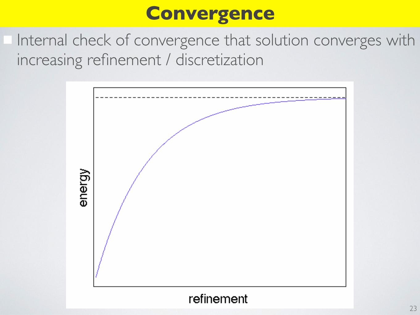
ConvergenceInternal check of convergence that solution converges with increasing refinement / discretization
23

Limitations and CaveatsApproximate solution with inherent errors
No closed form solution generated
Substantial experience / judgement required to synthesize good model
Computationally expensive
Data intensive I/O and computation
24
III. Simple Example
25
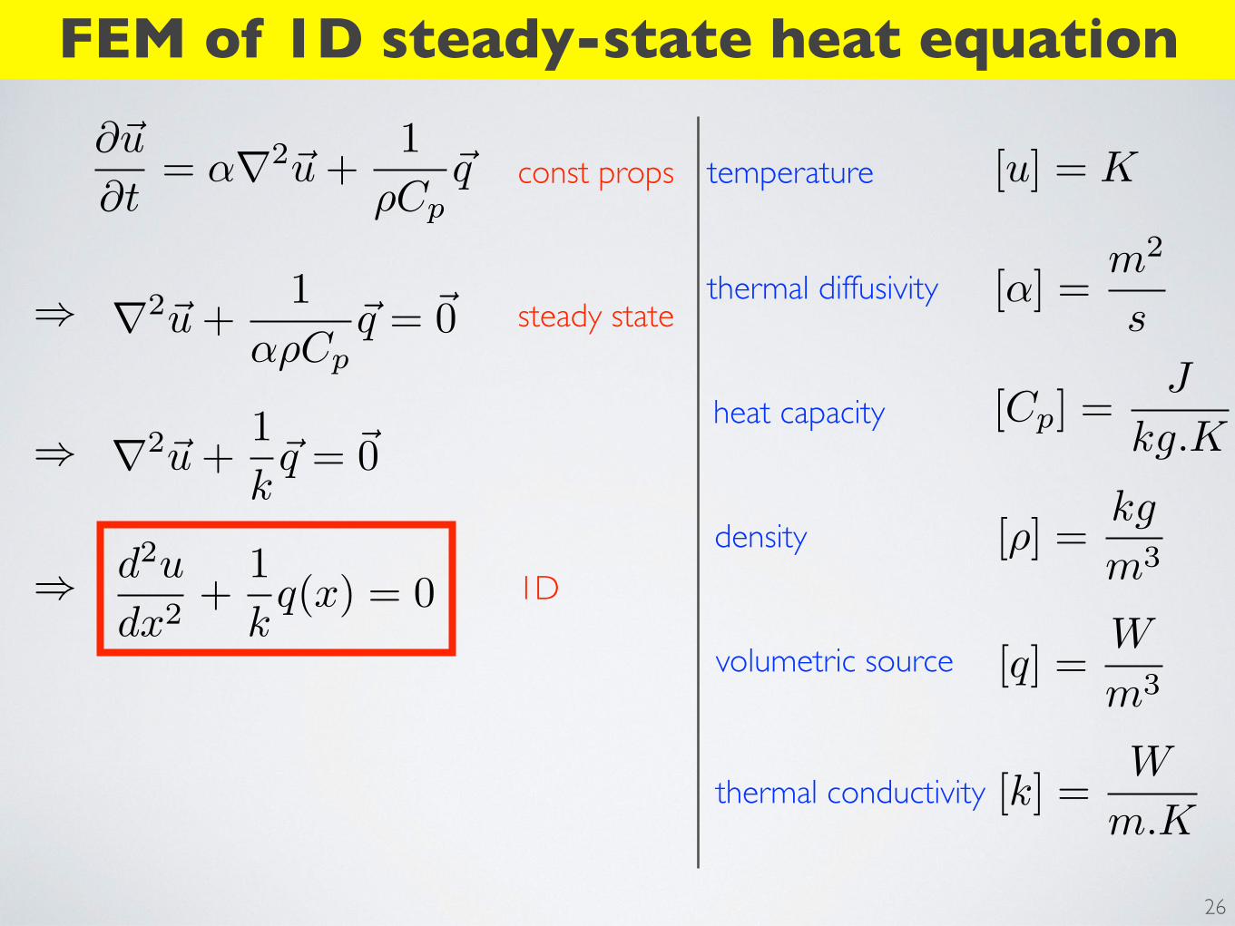
FEM of 1D steady-state heat equation
26
const props
steady state
1D
temperature
thermal diffusivity
heat capacity
density
volumetric source
thermal conductivity

System
27
x=0m x=1mxS=0.4m
T=0oC T=0oCC=4 kW/m3
k=57.8 W/m.K
Find steady-state temperature profile in the iron bar, u(x)

Analytical solution
28

1. Meshing
29
x=0 m x=1 m
II. Element properties
All elements identical size and thermal conductivity, k

III. Basis set
30
Simplest choice: “tent functions” - one-dimensional linear interpolants with compact support
http://www.panoramatech.com/papers/book/bookse11.php
y=1 n=4
Appropriate choice forproblem - expect linear soln
v1(x) v2(x) v3(x) v4(x)
u(x) =4X
i=1
uivi(x)
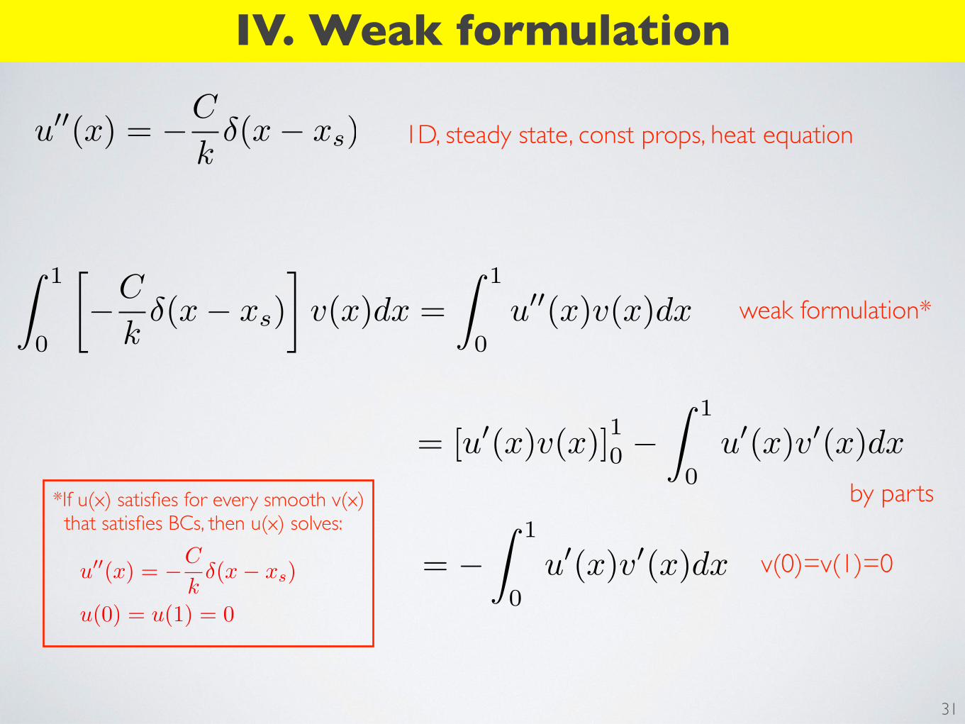
IV. Weak formulation
31
1D, steady state, const props, heat equation
weak formulation*
by parts
v(0)=v(1)=0
*If u(x) satisfies for every smooth v(x) that satisfies BCs, then u(x) solves:

IV. Weak formulation
32
governing eqn in each element
Exploiting finite support of each basis function:
Expanding solution in basis set:
Inserting solution expressed in basis set:
governing eqn in each element
ui are expansion coefficients

IV. Matrix form
33
governing eqn in each element
Finite dimensional basis admits simple matrix representation:
where
These matrix & vector elements can be explicitly evaluated!
“stiffness” matrix

IV. Matrix elements
34
Grinding through the (simple) algebra:
compactly supported basis functions make L sparse

Stiffness matrix is sparse, symmetric, and positive definite
Efficient solution via LU factorization or Cholesky decomposition
In MATLAB:
Recovering solution:
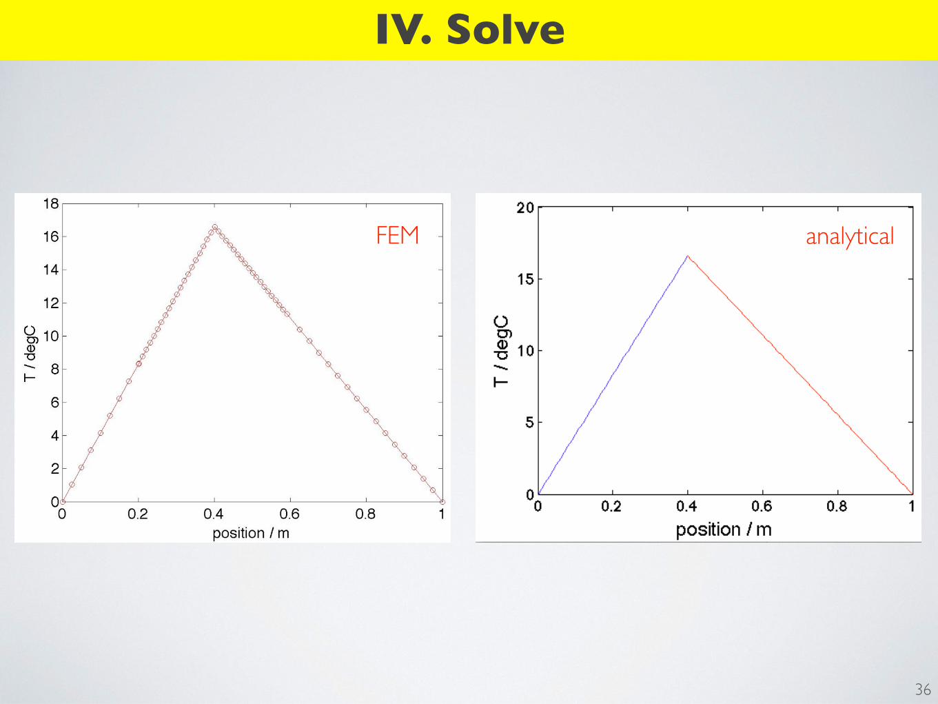
IV. Solve
35
General case - recover solution at arbitrary points x*:
u(x⇤) = up
✓xp+1 � x
⇤
xp+1 � xp
◆+ up+1
✓x
⇤ � xp
xp+1 � xp
◆
u(xp) = up
xp x
⇤< xp+1
Special case - recover solution only at grid points xp: ← very simple - the solution is the expansion coefficients!
u = �L\b
ui are expansion coefficients
vi are compactly supported, at most two are non-zero
IV. Solve
36
FEM analytical

IV. FEM Packages
37

FEM software
38
NIST FREEwww.ctcms.nist.gov/oof/oof2
Autodesk Simulation Multiphysics $4kwww.autodesk.com
Ansys UIUC lic.www.ansys.com
OOFEM FREEwww.oofem.org/en/oofem.html
Impact FREEhttp://impactprogram.wikispaces.com
CSC FREEwww.csc.fi/english/pages/elmer
Dassault Systemes $$$www.3ds.com/products-services/simulia
inuTech GmbH $$$www.diffpack.com


![Enhancements to Directional Coherence Maps · to the correct solution [Kajiy86]. The DCM incorpo-rate such a progressive refinement as well by using a hierarchical block refinement](https://img.dokumen.tips/doc/110x75/60a826d7679d92361a43c5d3/enhancements-to-directional-coherence-maps-to-the-correct-solution-kajiy86-the.jpg)