Evaluation of ensemble forecast uncertainty using a new ... · PDF fileQuarterlyJournaloftheRoyalMeteorologicalSociety Q.J.R.Meteorol.Soc.(2014)DOI:10.1002/qj.2375 Evaluation of ensemble

Quarterly Journal of the Royal Meteorological Society Q. J. R. Meteorol. Soc. (2014) DOI:10.1002/qj.2375

Evaluation of ensemble forecast uncertainty using a new proper score:Application to medium-range and seasonal forecasts

H. M. Christensen,a* I. M. Morozb and T. N. Palmera

aAtmospheric, Oceanic and Planetary Physics, University of Oxford, UKbOxford Centre for Industrial and Applied Mathematics, University of Oxford, UK

*Correspondence to: H. M. Christensen (nee H. M. Arnold), Atmospheric, Oceanic and Planetary Physics, Clarendon Laboratory,Parks Road, Oxford, OX1 3PU, UK. E-mail: [email protected]

Forecast verification is important across scientific disciplines, as it provides a frameworkfor evaluating the performance of a forecasting system. In the atmospheric sciences,probabilistic skill scores are often used for verification, as they provide a way of rankingthe performance of different probabilistic forecasts unambiguously. In order to be useful,a skill score must be proper: it must encourage honesty in the forecaster and rewardforecasts that are reliable and have good resolution. A new score, the error-spread score(ES), is proposed, which is particularly suitable for evaluation of ensemble forecasts. Itis formulated with respect to the moments of the forecast. The ES is confirmed to be aproper score and is therefore sensitive to both resolution and reliability. The ES is testedon forecasts made using the Lorenz ’96 system and found to be useful for summarizingthe skill of the forecasts. The European Centre for Medium-Range Weather Forecasts(ECMWF) ensemble prediction system (EPS) is evaluated using the ES. Its performanceis compared with a perfect statistical probabilistic forecast: the ECMWF high-resolutiondeterministic forecast dressed with the observed error distribution. This generates a forecastthat is perfectly reliable if considered over all time, but does not vary from day to day withthe predictability of the atmospheric flow. The ES distinguishes between the dynamicallyreliable EPS forecasts and the statically reliable dressed deterministic forecasts. Other skillscores are tested and found to be comparatively insensitive to this desirable forecast quality.The ES is used to evaluate seasonal range ensemble forecasts made with the ECMWFSystem 4. The ensemble forecasts are found to be skilful when compared with climatologicalor persistence forecasts, though this skill is dependent on the region and time of year.

Key Words: error-spread score; forecast verification; reliability; uncertainty; proper scores; ensemble forecasting

Received 15 July 2013; Revised 17 March 2014; Accepted 25 March 2014; Published online in Wiley Online Library

1. Intoduction: Evaluation of ensemble forecasts

It is well established that there are two major sources ofuncertainty in weather forecasts: initial condition uncertaintyand uncertainty due to the formulation of the weatherprediction model (Ehrendorfer, 1997). Instead of producing asingle deterministic forecast, an ensemble of forecasts shouldbe generated in which the ensemble members explore theseuncertainties (Palmer, 2001). The resultant probabilistic forecastis then issued to the user, who can make better informed decisionsthan if no uncertainty estimate were available. There are manydifferent methods commonly used for verification of probabilisticforecasts. Graphical forecast verification techniques provide acomprehensive summary of the forecast, but it can be difficultto compare many forecast models using them. They can also bemisleading, so must be interpreted carefully to draw the correctconclusions (Hamill, 2001). Instead, it is often necessary to choosea scalar summary of forecast performance which allows several

forecasts to be ranked unambiguously. Scoring rules provide aframework for forecast verification. They summarize the accuracyof the forecast by giving a quantitative score based on the forecastprobabilities and the actual outcome and can be considered asrewards that a forecaster wants to maximize.

Scoring rules must be carefully designed to encourage honestyfrom the forecaster: they must not contain features that promoteexaggerated or understated probabilities. This constitutes a properscore, without which the forecaster may feel pressurized to presenta forecast that is not their best guess (Brown, 1970). For example,a forecaster may want to be deliberately vague such that his orher prophecy will be proved correct, regardless of the outcome.Specifically, a proper scoring rule is one that is optimized ifthe true probability distribution is predicted, whereas a score isstrictly proper if it is optimized if and only if the true distributionis predicted.

Ideally, the verification should behave like a randomsample from the forecast probability distribution function (pdf)

c© 2014 Royal Meteorological Society

H. M. Christensen et al.

(Anderson, 1997; Wilks, 2006). If this is the case, the ensembleis perfectly capturing the uncertainty in the forecast and theforecast is said to be reliable. However, when averaged over along enough time window, the climatological forecast is perfectlyreliable but could be considered not to be particularly skilful forweather applications. The additional property that a probabilisticforecast must possess is resolution. Resolution is the propertythat provides the forecaster with information specifying thefuture state of the system (Brocker, 2009). Resolution is aproperty of the joint distribution of forecasts and observations:to have high resolution, a forecast must sort the observed statesof the system into groups that are different from each other(Wilks, 2006; Leutbecher, 2010). A proper skill score mustevaluate both the reliability and the resolution of a probabilisticforecast.

Currently, many scoring rules used for forecast verification,such as the continuous ranked probability score (CRPS: Wilks,2006) and the ignorance score (IGN: Roulston and Smith, 2002),require an estimate of the full forecast pdf. This is usually achievedusing kernel smoothing estimates or by fitting the parameters insome predetermined distribution, both of which require certainassumptions about the forecast pdf to be made. Alternatively, thepdf must be discretized in some way, such as for the Brier score(BS) and ranked probability score (RPS) (Wilks, 2006), whichwere both originally designed for multi-category forecasts. Onthe other hand, comparing the root-mean-square (RMS) errorin the ensemble mean with the ensemble spread (Leutbecherand Palmer, 2008; Leutbecher, 2010) is an attractive verificationtool, as it does not require an estimation of the full forecast pdfand instead is calculated using the raw ensemble forecast data.The RMS error and spread are displayed on scatter diagramsfor subsamples of the forecast cases conditioned on the spread.This diagnoses the ability of the forecasting system to make flow-dependent uncertainty estimates. However, being a graphicaldiagnostic, it is very difficult to compare many forecast modelsusing this tool.

We propose a new scoring rule designed for ensemble forecastsof continuous variables that is particularly sensitive to thereliability of a forecast and seeks to summarize the RMS error-spread scatter diagnostic. It will be formulated with respect tomoments of the forecast distribution and not using the fulldistribution itself. These moments may be calculated directlyfrom the ensemble forecast, provided it has sufficient membersfor an accurate estimate to be made. The new score we proposedoes not require the forecast to be discretized and acknowledgesthe inability of the forecaster to specify a probability distributionfor a variable fully, due both to the amount of information neededto estimate the distribution and the number of bits needed torepresent it on a computer. This limitation has been recognizedby other authors and forms the basis for the development of Bayeslinear statistics (Goldstein and Wooff, 2007).

The new score will be compared with a number of existingproper scores, detailed below.

1.1. The Brier score

The BS (Wilks, 2006) is used when considering dichotomousevents (e.g. rain or no rain). It is the mean square differencebetween the forecast and observed probability of an eventoccurring:

BSi = (yi − oi)2, (1)

where yi is the ith predicted probability of the event occurring;oi = 1 if the event occurred and 0 otherwise. The BS must beevaluated for many test cases i and the arithmetic mean calculated.

The BS can be decomposed explicitly into its reliabilityand resolution components (Murphy, 1973). In particular, the

reliability component of the BS is given by

REL = 1

N

P∑p=1

np

(fp − op

)2, (2)

where N is the total number of forecast–observation pairsand P is the number of unique forecast probabilities issued;for example, P = 11 if the allowed forecast probabilities are[0.0, 0.1, 0.2, . . . , 1.0]. fp is the forecast probability, op is theobserved frequency of the event given that fp was forecast and np

is the number of times fp was forecast.

1.2. The ranked probability score

The RPS is used to evaluate a multi-category forecast. Suchforecasts can take two forms: nominal, where there is no naturalordering of events, and ordinal, where the events are orderednumerically. For ordinal predictions, it is desirable that the scoretakes the ordering into account: a forecast should be rewardedfor allocating high probabilities to events similar in magnitudeto the observed event (a close distance in variable space). TheRPS is defined as the squared sum of the difference betweenforecast and observed probabilities, so is closely related to theBS. However, in order to include the effects of distance discussedabove, the difference is calculated between the cumulative forecastprobabilities Ym,i and the cumulative observations Om,i (Wilks,2006). Defining the number of event categories to be J, the ithforecast probability for event category j to be yj,i and the ithobserved probability for event category i to be oj,i,

Ym,i =m∑

j=1

yj,i, m = 1, 2, . . . , J (3)

and

Om,i =m∑

j=1

oj,i, m = 1, 2, . . . , J, (4)

then

RPSi =J∑

m=1

(Ym,i − Om,i)2 (5)

and the average RPS is calculated over many test cases i. In thisarticle, ten event categories are used, defined as the deciles of theclimatological distribution.

1.3. Ignorance

IGN was proposed by Roulston and Smith (2002) as a wayof evaluating a forecast based on the information it contains.As for the RPS, we define J event categories and considerN forecast–observation pairs. The forecast probability thatthe ith verification will be event j is defined to be f (i)j

(where j = 1, 2, . . . , J and i = 1, 2, . . . , N). If the correspondingoutcome event was j(i), IGN is defined to be

IGNi = −log2f (i)j(i). (6)

IGN should be calculated by averaging over many forecast-verification pairs. As for the RPS, the deciles of the climatologicaldistribution are used in this work to define ten categories forevaluating IGN. The expected value of IGN is closely related tothe relative entropy of the forecast,

R =∑

i

pi ln

(pi

qi

), (7)

c© 2014 Royal Meteorological Society Q. J. R. Meteorol. Soc. (2014)

Evaluation of Ensemble Forecast Uncertainty

where qi is the climatological distribution and pi is the forecast dis-tribution (Roulston and Smith, 2002). Information theoretic mea-sures, such as relative entropy and therefore IGN, measure forecastutility and have been shown to be useful for quantifying pre-dictability in chaotic systems (Kleeman, 2002; Majda et al., 2002).

1.4. Skill scores

Each of the above scores (S) may be converted into a skill score(SS) by comparison with the score evaluated for a referenceforecast, Sref :

SS = (S − Sref )

(Sperf − Sref ). (8)

For all the scoring rules above the perfect score, Sperf is zero andthe skill score can be expressed as

SS = 1 − S

Sref, −∞ < SS ≤ 1. (9)

2. The error-spread score

Consider two distributions. Q(X) is the truth probabilitydistribution function, which has moments mean µ, varianceσ 2, skewness γ and kurtosis β , defined in the usual way:

µ = E[X], (10)

σ 2 = E[(X − µ)2], (11)

γ = E

[(X − µ

σ

)3]

, (12)

β = E

[(X − µ

σ

)4]

, (13)

where E[·] denotes the expectation of the variable. Theprobabilistic forecast issued is denoted P(X), with mean m,variance s2, skewness g and kurtosis b, defined in the sameway. The perfect probabilistic forecast will have moments equalto those of the truth distribution: m = µ, s2 = σ 2, g = γ andb = β , etc.

The error-spread score (ES) is written

ESi = (s2i − e2

i − eisigi)2, (14)

where the difference between the verification zi and the ensemblemean mi is the error in the ensemble mean,

ei = (mi − zi), (15)

and the verification zi follows the truth probability distribution Q.The ES is calculated by averaging over many forecast-verificationpairs i, both from different grid-point locations and from differentstarting dates. A smaller average value of the score indicates abetter set of forecasts.

The first two terms in the square of the right-hand side ofEq. (14) are motivated by the spread-error relationship; for areliable ensemble, it is expected that the ensemble variance, s2,will give an estimate of the expected squared error in the ensemblemean, e2 (Leutbecher and Palmer, 2008). However, with thesetwo terms alone, the score is not proper.∗ Consider the trial score,

∗Note that the relationship between the average spread and average squareerror is valid for any distribution, regardless of skewness (Leutbecher andPalmer, 2008). However, skewness becomes important when the instantaneousvalues of spread and error are compared, as in the ES.

Figure 1. Schematic illustrating how the ES accounts for the skewness of theforecast distribution. The hypothetical probability density function (pdf) shownas a function of X is positively skewed and has mean (m) and standard deviation(s) as indicated. See text for more details.

(dropping the subscript i):

EStrial = (s2 − e2)2. (16)

It can be shown that the expected value of this score is notminimized by predicting the true moments m = µ, s = σ .In fact it is minimized by forecasting m = µ + γ σ/2 ands2 = σ 2

(1 + γ 2/4

)(see Appendix A). The substitutions

m → m + gs/2 and s2 → s2(1 + g2/4

)transform the trial

score into the ES (Eq. (14)), which can be shown to be a properscore (section 3).

The third term in the ES can be understood as acknowledgingthat the full forecast pdf contains more information than is inthe first two moments alone. This term depends on the forecastskewness, g. Consider the case when the forecast distributionis positively skewed (Figure 1). If the observed error is smallerthan the predicted spread, e2 < s2, the verification must fall ineither section B or C in Figure 1. The skewed forecast distributionpredicts that the verification is more likely to fall in B, so this caseis rewarded by the scoring rule. If the observed error is larger thanthe predicted spread, e2 > s2, the verification must fall in eithersection A or section D in Figure 1. Now, the forecast pdf indicatesthat section D is the more likely of the two, so the scoring rulerewards a negative error e.

The ES is a function of the first three moments only. Thiscan be understood by considering Eq. (16). When expanded, theresultant polynomial is fourth-order in the verification z. Thecoefficient of the z4 term is unity, i.e. it is dependent on the fourthpower of the verification only, so the forecaster cannot hedge hisor her bets by altering the kurtosis of the forecast distribution. Thefirst term with a non-constant coefficient is the z3 term, indicatingthat skewness is the first moment of the true distribution thatinteracts with the forecaster’s prediction. The forecast skewnessis therefore important and should appear in the proper score. Ifthe score were based on higher powers, for example motivatedfrom (sn − en)2, the highest-order moment required would bethe (2n − 1)th moment.†

3. Propriety of the error-spread score

A scoring rule must be proper in order to be a useful measureof forecast skill. The ES cannot be strictly proper, as it is onlya function of the moments of the forecast distribution; a pdfwith the same moments as the true pdf will score equallywell. However, it is important to confirm that the ES is aproper score.

To test for propriety, we calculate the expected value of thescore, assuming the verification follows the truth distribution

†Scores based on the magnitude of the error were also considered, for example(|s| − |e|)2, but a proper score could not be found.



(refer to Appendix B for the full derivation).

E [ES] = [(σ 2 − s2) + (µ − m)2 − sg(µ − m)

]2

+ σ 2[2(µ − m) + (σγ − sg)

]2

+ σ 4(β − γ 2 − 1). (17)

In order to be proper, the expected value of the scoringrule must be minimized when the truth distribution is forecast.Appendix B confirms that the truth distribution falls at a stationarypoint of the score, and that this stationary point is a minimum.Therefore the scoring rule is proper, though not strictly proper,and is optimized by issuing the truth distribution. Appendix Balso includes a second test of propriety, from Brocker (2009).

4. Testing the error-spread score using the gammadistribution

To analyze the sensitivity of the score to properties of theforecast and to demonstrate in what way it differs from existingscores, the ES score is first tested using an idealized statisticaldistribution. The gamma distribution is a family of continuousprobability distributions. The probability density function is givenby f (x;α, θ):

f (x;α, θ) = (x − M)α−1e−(x−M)/θ

θα�(α), (18)

where �(α) is the gamma function evaluated at α and(x − M), α, θ > 0. The gamma distribution has mean m =αθ + M, standard deviation s = θ

√α and skewness g = 2/

√α;

the gamma distribution is a useful test case for the ES, as itis a skewed distribution. The verification is defined to be arandom number drawn from a gamma distribution with moments(m, s, g) = (10, 6, 1.3). The error-spread skill score (ESS), Brierskill score (BSS), ranked probability skill score (RPSS) andignorance skill score (IGNSS) are used to evaluate many differentidealized forecasts. Each 300 member ensemble forecast is drawnfrom the gamma distribution with moments (mfc, sfc, gfc), whichare not necessarily equal to those for the ‘true’ verification gammadistribution. This is repeated for 10 000 test cases and the skillscores averaged over all cases.

Figure 2 shows each score evaluated as a function of the meanand spread of the forecast gamma distribution. The scores areconverted to skill scores by comparison with the climatologicalforecast (the true gamma distribution). As expected, each scoreindicates that forecasting a gamma distribution with the ‘true’moments is the most skilful.

The BSS is very sensitive to the mean of the forecast distributionand penalizes biased forecasts which have a systematic error in themean. However, it is comparatively insensitive to the spread of

the forecast distribution: it cannot distinguish between unbiasedforecasts that are under- or overdispersive. The RPSS is alsoless sensitive to the forecast spread than to the forecast bias.The IGNSS is assymetric and penalizes underdispersive forecastsheavily, but does not penalize overdispersive forecasts heavily.The ESS is sensitive to both the forecast mean and spread andevenly penalizes forecasts that have either moment incorrect:the contours are approximately circular. Similar figures can beused to explore the other directions in (m, s, g) space: the ESS isfound to be more sensitive to skewness than the other scores (notshown).

For a reliable forecast, it is important that the ensemble has thecorrect second moment. If it is underdispersive, the verificationwill frequently fall as an outlier. Conversely, if the ensemble isoverdispersive, the verification may fall too often towards thecentre of the distribution. The ESS is more sensitive to thesecond moment of the forecast than the other scores tested here,indicating an increased sensitivity to the reliability of a forecast.

5. Testing the error-spread score: Evaluation of forecastsin the Lorenz ’96 system

Experiments are carried out in the Lorenz (1996, hereafter L96)simplified model of the atmosphere. The model consists of twoscales of variables: a ring of large-scale, low-frequency X variablescoupled to many smaller scale high-frequency Y variables. Theinteraction between these scales is described by the set of coupledequations

dXk

dt= −Xk−1(Xk−2 − Xk+1) − Xk + F (19a)

− hc

b

kJ∑j=J(k−1)+1

Yj; k = 1, . . . , K,

dYj

dt= −cbYj+1(Yj+2 − Yj−1) − cYj (19b)

+ hc

bXint[(j−1)/J]+1; j = 1, . . . , JK,

where the variables have cyclic boundary conditions: Xk+K = Xk

and Yj+KJ = Yj. The interpretation of the parameters in theseequations and the values used in this study are shown in Table 1.The scaling of the variables is such that one model time unit isequal to five atmospheric days, deduced by comparing the errordoubling time of the model with that observed in the atmosphere(Lorenz, 1996).

This model provides an excellent test bed for techniques inatmospheric modelling, as a robust ‘truth’ can be defined touse as a verification. The full two-scale model is run and theresultant X time series defined as truth. A simplified model inwhich the Y variables are assumed unresolved is also run to

mfc

s fc

ESS(a)

8 10 124

5

6

7

8

−0.5 0

mfc

s fc

BSS(b)

8 10 124

5

6

7

8

−0.1 −0.05 0

mfc

s fc

RPSS(c)

8 10 124

5

6

7

8

−0.2 −0.1 0

mfc

s fc

IGNSS(d)

8 10 124

5

6

7

8

−0.5 0

Figure 2. (a) Error-spread skill score, (b) Brier skill score, (c) ranked probability skill score and (d) ignorance skill score evaluated for gamma distribution forecasts.The verification is drawn from a gamma distribution with moments (m, s, g) = (10, 6, 1.3), indicated by a black cross in each panel. The ensemble forecast is drawnfrom a gamma distribution with moments (mfc, sfc, gfc) indicated by the axis labels. The third moment gfc = g = 1.3 for each figure.



Table 1. Parameter settings used for the L96 system.

Parameter Symbol Setting

No. X variables K 8No. Y variables per X variable J 32Coupling constant h 1Forcing term F 20Spatial scale ratio b 10Time-scale ratio c 10

Table 2. Tunable parameters in the forecast model for the L96 system and theirvalues fitted from the truth time series.

a0 a1 a2 a3 σn φ

0.359 1.31 −0.0146 −0.00230 1.99 0.985

produce forecasts of the state of the X variables. The forecastmodel is given by Eq. (20): the effect of the unresolved Y variableson the X variables is represented by a cubic polynomial inX and a first-order autoregressive (AR(1)) additive stochastic

term is included to represent the variability of the unresolved Yvariables.

dXk

dt= −Xk−1(Xk−2 − Xk+1) − Xk + F − U(Xk), (20a)

U(Xk) = a0 + a1Xk + a2X2k + a3X3

k + ek(t), (20b)

ek(t) = φek(t − �t) + σn(1 − φ2)0.5z(t). (20c)

The cubic fit constants ai, the standard deviation of the noise termσn and the autocorrelation of the noise term φ are determinedfrom the truth time series and their fitted values are given inTable 2. The random number z(t) ∼ N (0, 1). For more detailson the methodology and for experiments using more complicatedstochastic forecast models, refer to Arnold et al. (2013).

40 member ensemble forecasts were initialized from perfectinitial conditions and their forecast skill evaluated at a lead timeof 0.9 model time unit (∼4.5 atmospheric days). The tunableparameters in the forecast model, σn and φ, were varied and theforecasts for each parameter pair evaluated using three techniques.Figure 3(a) shows the graphical error-spread diagnostic. Theforecast-verification pairs are binned according to the variance ofthe forecast. The average variance in each bin is plotted against

0 20 400

20

40

MS Spread

MS

Err

or

0 20 40 0 20 40 0 20 40 0 20 40 0 20 40

0

20

400

20

400

20

400

20

400

20

40(a)

0.0010.003

0.003

0.005

0.005

0.001

0.007

0.009

0.003

φ

σ / σ

mea

s

0.00

0

0.60

7

0.88

2

0.96

9

0.99

3

0.99

8

(b)

0.0

0.5

1.0

1.5

2.0

2.50.760.780.8

0.82

0.840.860.88

0.9

0.9

0.9

0.92

0.92

0.920.94

0.94

0.94

φ

σ / σ

mea

s

0.00

0

0.60

7

0.88

2

0.96

9

0.99

3

0.99

8

(c)

0.0

0.5

1.0

1.5

2.0

2.5

0.607 0.882 0.969 0.993 0.9980.000φ

2.5

2.0

1.5

1.0

0.5

0.0

σ / σm

Figure 3. (a) The mean square (MS) error-spread diagnostic, (b) the reliability component of the Brier score and (c) the error-spread skill score, evaluated forforecasts of the L96 system using an additive stochastic parametrization scheme. In each figure, moving left–right, the autocorrelation of the noise in the forecastmodel, φ, increases. Moving bottom–top, the standard deviation of the noise, σn, increases. The individual panels in (a) correspond to different values of (φ, σm). Thebottom row of panels in (a) are blank because deterministic forecasts cannot be analyzed using the MS error-spread diagnostic: there is no forecast spread to conditionthe binning on.



0 4.5 9 13.5 18 22.5289

290

291

292

293

294

295

Longitude

T 8

50

(a) EPS: 4° N

0 4.5 9 13.5 18 22.5289

290

291

292

293

294

295

Longitude

(b) DD: 4° N

13.3 20 26.7 33.3 40 46.7

250

260

270

280

290

300

Longitude

(c) EPS: 53° N

13.3 20 26.7 33.3 40 46.7

250

260

270

280

290

300

Longitude

(d) DD: 53° N

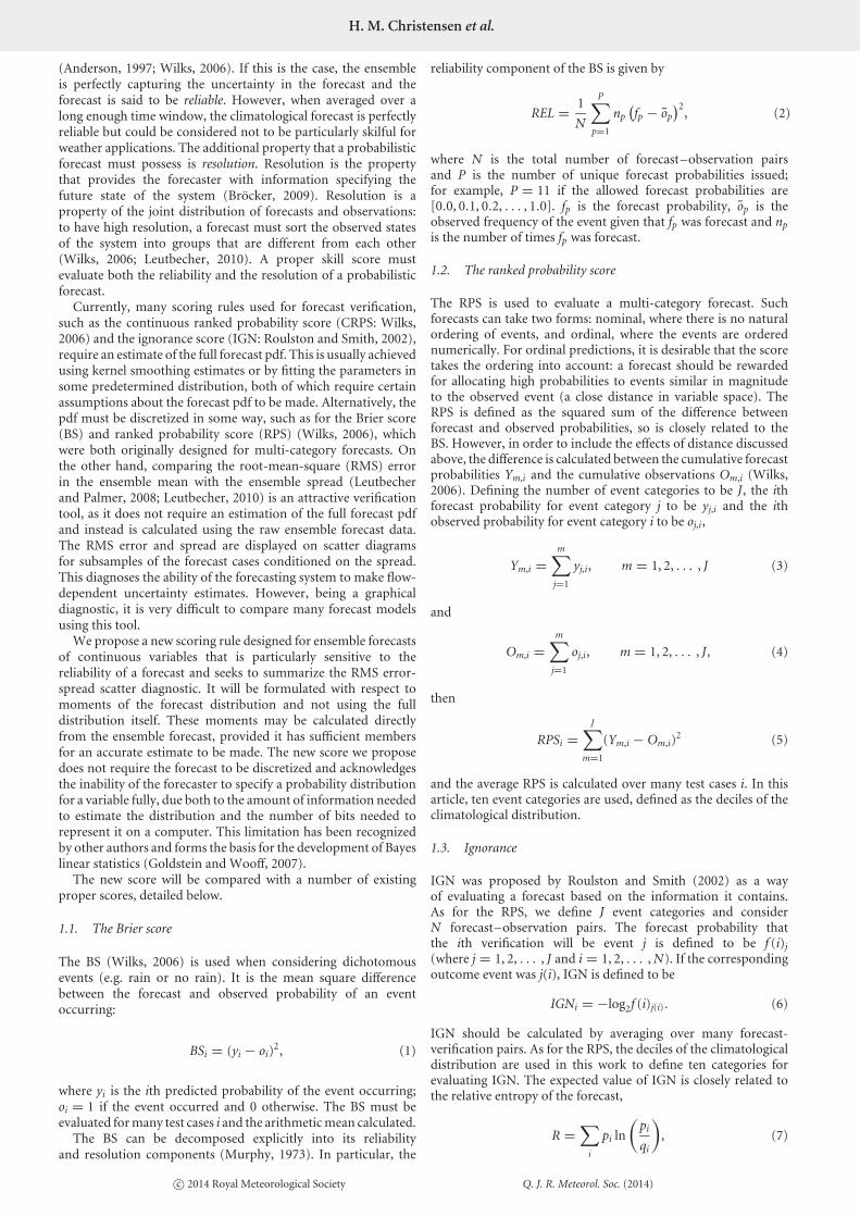
Figure 4. 4DVar analyses (black) of temperature at 850 hPa (T850) are compared with the ten-day ensemble forecasts (grey) at 11 longitudes at 4◦N for (a) the EPSand (b) the dressed deterministic system and at 11 longitudes at 53◦N for (c) the EPS and (d) the dressed deterministic system. The forecasts are initialized on 19 April2012 for all cases. The horizontal black dashed lines correspond to the deciles of the climatological distribution of T850 at this latitude.

the mean square error in each bin. For a reliable forecast system,these points should lie on the diagonal (Leutbecher and Palmer,2008). Figure 3(b) shows the reliability component of the Brierscore (Brier, 1950; Murphy, 1973), REL (Eq. (2)), where the‘event’ was defined as ‘the Xk variable is in the top third of itsclimatological distribution’. Figure 3(c) shows the new error-spread skill score (ESS), which is calculated with respect to theclimatological forecast.

The difficulty of analyzing many forecasts using a graphicalmethod can now be appreciated. Trends can easily be identifiedin Figure 3(a), but the best set of parameter settings is hardto identify. The stochastic forecasts with small-magnitude noise(low σn) are underdispersive. The error in the ensemble meanis systematically larger than the spread of the ensemble, i.e.they are overconfident. However, the stochastic parametrizationswith very persistent, large-magnitude noise (large σn, large φ)are overdispersive. Figure 3(b) shows REL evaluated for eachparameter setting, which is small for a reliable forecast. It scoreshighly those forecasts where the variance matches the mean squareerror, such that the points in (a) lie on the diagonal. The ESS is aproper score and is also sensitive to the resolution of the forecast.It rewards well-calibrated forecasts, but also those that have asmall error. The peak of the ESS in Figure 3(c) is shifted downcompared to REL and it penalizes the large σn, large φ models forthe increase in error in their forecasts. The ESS has summarizedthe results in Figure 3(a) and has shown a sensitivity to bothreliability and resolution, as required of a proper score.

6. Testing the error-spread score: Evaluationof medium-range forecasts from the integrated forecastingsystem

The ESS was tested using 10 day operational forecasts madewith the European Centre for Medium-Range Weather Forecasts(ECMWF) Ensemble Prediction System (EPS). The EPS usesa spectral atmosphere model, the Integrated Forecasting System(IFS). Out to day 10, the EPS is operationally run with a horizontaltriangular truncation of T639,‡ with 62 vertical levels, and usespersisted sea-surface temperature (SST) anomalies instead ofa dynamical ocean model. The 50 member ensemble samplesinitial condition uncertainty using perturbations derived froman ensemble of data assimilations (EDA: Isaksen et al., 2010),which are combined with perturbations from the leading singularvectors (Buizza et al., 2008).

The EPS system uses stochastic parametrizations to representuncertainty in the forecast due to model deficiencies; the50 ensemble members differ, as each uses a different seedfor the stochastic parametrization schemes. Two stochasticparametrization schemes are used. The stochastically perturbed

‡The IFS is a spectral model and resolution is indicated by the wave number atwhich the model is truncated. For comparison, a spectral resolution of T639corresponds to a reduced Gaussian grid of N320, or 30 km resolution, or a0.28◦ latitude/longitude grid.

parametrization tendencies (SPPT) scheme (Palmer et al., 2009)addresses model uncertainty due to physical parametrizationschemes; it perturbs the parametrized tendencies about theaverage value that a deterministic scheme represents. In SPPT,the parametrized tendencies in the horizontal wind components,temperature and humidity are multiplied by a random number.A spectral pattern generator is used to generate a smoothlyvarying perturbation field and the pattern’s spectral coefficientsevolve in time according to an AR(1) process. The secondscheme, stochastic kinetic energy backscatter (SKEB: Berneret al., 2009), represents a physical process absent from theIFS deterministic parametrization schemes. In SKEB, randomstream-function perturbations are used to represent upscalekinetic energy transfer. This counteracts the kinetic energy lossfrom too much dissipation in numerical integration schemes.The same kind of pattern generator as used in SPPT modulatesthe perturbations to the stream functions.

Ten-day forecasts were considered, initialized from 30 datesbetween 14 April and 15 September 2012 and separatedfrom each other by 5 days. The high-resolution 4D variational(4DVar) analysis (T1279, 16 km) was used for verification. Bothforecast and verification fields were truncated to T159 (125 km)before verification. Forecasts of temperature at 850 hPa (T850,approximately 1.5 km above ground level) were considered andthe RPS, IGN and ES calculated for each grid point for eachtest date. Each score was calculated as a function of latitude byaveraging over all test dates and grid points in a particular latitudeband.

For comparison, a perfect static probabilistic forecast wasgenerated based on the high-resolution (T1279, 0.141◦)operational deterministic forecast. This is defined in an analagousway to the idealized hypothetical forecasts in Leutbecher (2010).The error between the deterministic forecast and the 4DVaranalysis is computed for each ten-day forecast and the error pdfcalculated as a function of latitude. Each deterministic forecast isthen dressed with a 50 member ensemble of errors drawn from thislatitudinally dependent distribution. This dressed deterministicensemble (DD) can be considered a ‘perfect statistical’ forecast,as the error distribution is correct if averaged over all time,but it does not vary from day to day, as the predictability ofthe atmospheric flow varies. A useful score should distinguishbetween this perfect static forecast and the dynamic probabilisticforecasts made using the EPS.

An example ten-day forecast using these two systems is shownin Figure 4 for 11 longitudes close to the Equator and for 11longitudes in the midlatitudes. The flow dependence of the EPSis evident: the spread of the ensemble varies with position, givingan indication of the uncertainty in the forecast. The spread of theDD ensemble varies slightly, indicating the sampling error for a50 member ensemble.

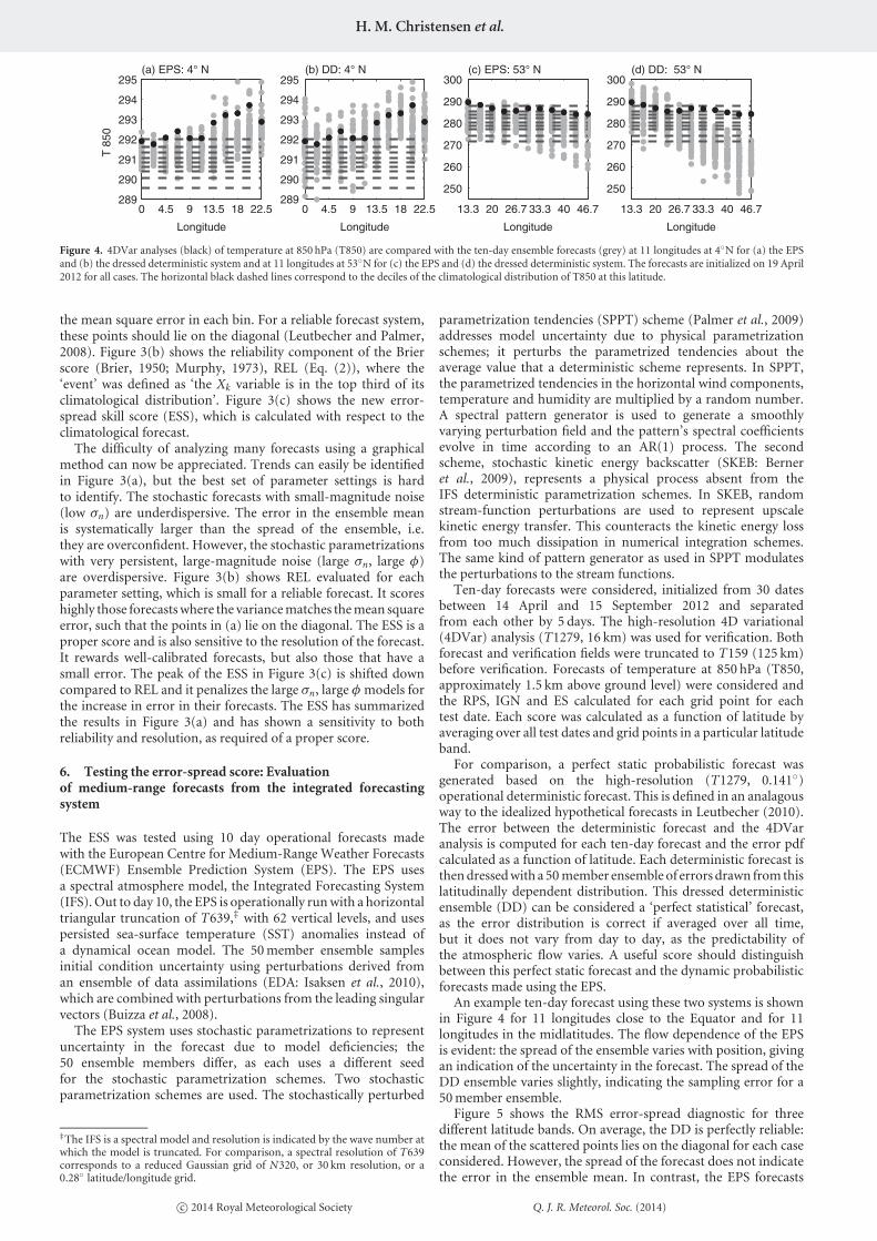
Figure 5 shows the RMS error-spread diagnostic for threedifferent latitude bands. On average, the DD is perfectly reliable:the mean of the scattered points lies on the diagonal for each caseconsidered. However, the spread of the forecast does not indicatethe error in the ensemble mean. In contrast, the EPS forecasts



0 1 2 30

1

2

3

RMS Spread

RM

S E

rror

(a) 18S − 10S

0.2 0.4 0.6 0.8 1 1.20.2

0.4

0.6

0.8

1

1.2

RMS Spread

RM

S E

rror

(b) 0N − 8N

2 4 61

2

3

4

5

6

RMS Spread

RM

S E

rror

(c) 50N − 60N

Figure 5. RMS error-spread plot for forecasts made using the EPS (pale grey) and the DD system (dark grey). Ten-day forecasts of T850 are considered for latitudesbetween (a) 18◦S and 10◦S, (b) 0◦N and 8◦N and (c) 50◦N and 60◦N. The ensemble forecasts are sorted and binned according to their forecast spread. The RMS errorin the ensemble mean in each bin is plotted against the RMS spread for each bin. For a reliable ensemble, these should lie on the diagonal shown (Leutbecher andPalmer, 2008).

5 10 15 20 25 30 35 40 45 501

1.1

1.2

1.3

1.4

1.5

1.6

1.7

1.8

M

S/S

M=

50

ESRPSIGN

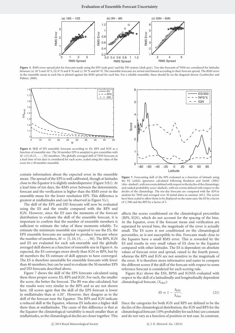
Figure 6. Skill of IFS ensemble forecasts according to ES, RPS and IGN as afunction of ensemble size. The 50 member EPS is sampled to give ensembles withM =[5,10,15, . . . , 50] members. The globally averaged skill of T850 forecasts ata lead time of ten days is considered for each score, scaled using the value of thescore for a 50 member ensemble.

contain information about the expected error in the ensemblemean. The spread of the EPS is well calibrated, though at latitudesclose to the Equator it is slightly underdispersive (Figure 5(b)). Ata lead time of ten days, the RMS error between the deterministicforecast and the verification is higher than the RMS error in theensemble mean for the lower resolution EPS. This difference isgreatest at midlatitudes and can be observed in Figure 5(c).

The skill of the EPS and DD forecasts will now be evaluatedusing the ES and the results compared with the RPS andIGN. However, since the ES uses the moments of the forecastdistribution to evaluate the skill of the ensemble forecast, it isimportant to confirm that the number of ensemble members issufficient to estimate the value of these moments reliably. Toestimate the minimum ensemble size required to use the ES, theEPS ensemble forecasts are sampled to produce forecasts wherethe number of members, M = [5, 10, 15, . . . , 50]. The RPS, IGNand ES are evaluated for each sub-ensemble and the globallyaveraged skill shown as a function of ensemble size in Figure 6. Asexpected, the ES converges more slowly than IGN or RPS, but by40 members the ES estimate of skill appears to have converged.The ES is therefore unsuitable for ensemble forecasts with fewerthan 40 members, but can be used to evaluate the 50 member EPSand DD forecasts described above.

Figure 7 shows the skill of the EPS forecasts calculated usingthese three proper scores: ES, RPS and IGN. For each, the smallerthe score, the better the forecast. The BS was also calculated, butthe results were very similar to the RPS and so are not shownhere. All scores agree that the skill of the EPS forecast is lowerin midlatitudes than at ±20◦. However, they disagree as to theskill of the forecast near the Equator. The RPS and IGN indicatea reduced skill at the Equator, whereas ES indicates a higher skillthere than at midlatitudes. The cause of this difference is that atthe Equator the climatological variability is much smaller than atmidlatitudes, so the climatological deciles are closer together. This

−80 −60 −40 −20 0 20 40 60 800

1

2

3

4

5

6

Latitude

Sco

re

ES/300RPS*5IGN

Figure 7. Forecasting skill of the EPS evaluated as a function of latitude usingthe ES (solid); ignorance calculated following Roulston and Smith (2002)(dot–dashed), with ten events defined with respect to the deciles of the climatology;and ranked probability score (dashed), with ten events defined with respect to thedeciles of the climatology. The ten-day forecasts are compared with the 4DVaranalysis for T850 and averaged over 30 initial dates in summer 2012. The scoreshave been scaled to allow them to be displayed on the same axes: the ES by a factorof 1/300 and the RPS by a factor of 5.

affects the scores conditioned on the climatological percentiles(RPS, IGN), which do not account for the spacing of the bins.At the Equator, even if the forecast mean and verification areseparated by several bins, the magnitude of the error is actuallysmall. The ES score is not conditioned on the climatologicalpercentiles, so is not susceptible to this. Forecasts made close tothe Equator have a small RMS error. This is rewarded by theES and results in very small values of ES close to the Equatorcompared with other latitudes. The ES is dependent on absolutevalues of forecast error and spread, raised to the fourth power,whereas the RPS and IGN are not sensitive to the magnitude ofthe error. It is therefore more informative and easier to comparethe different scores if the skill of the forecast with respect to somereference forecast is considered for each scoring rule.

Figure 8(a) shows the ESS, RPSS and IGNSS evaluated withrespect to the skill of a latitudinally and longitudinally dependentclimatological forecast, (Sclim):

SS = 1 − SEPS

Sclim. (21)

Since the categories for both IGN and RPS are defined to be thedeciles of the climatological distribution, the IGN and RPS for theclimatological forecast (10% probability for each bin) are constantand do not vary as a function of position or test case. In constrast,



−80−60−40−20 0 20 40 60 80

−0.2

0

0.2

0.4

0.6

0.8(a)

Reference: Climatology

Latitude

Ski

ll S

core

−80−60−40−20 0 20 40 60 80

−0.2

0

0.2

0.4

0.6

0.8(b)

Reference: DD

Latitude

Ski

ll S

core

−80−60−40−20 0 20 40 60 80

−0.2

0

0.2

0.4

0.6

0.8

Latitude

Ski

ll S

core

(c)Reference: DEM

ESSRPSSIGNSS

Figure 8. Skill scores for the EPS forecast evaluated as a function of latitude using (a) the climatological forecast as a reference, (b) the dressed deterministic forecastas a reference and (c) the dressed deterministic forecast as a reference, where the ensemble mean is used as the deterministic forecast. Three proper skill scores arecalculated: the ESS (solid), ignorance calculated following Roulston and Smith (2002) (dot–dashed) and RPSS (dashed). The legend in (c) corresponds to all figures.The ten-day forecasts are compared with the 4DVar analysis for T850 and averaged over 30 initial dates in the summer of 2012.

the ES for the climatological forecast is strongly latitudinallydependent, as the ES is sensitive to the absolute magnitudes ofthe forecast distribution: an ensemble forecast with small spreadand small forecast error will score better than a forecast withlarge spread and large error. Despite these differences, when eachskill score is calculated, all three proper skill scores rank differentlatitudes similarly. All three skill scores indicate little or no skill forforecasts made near the Equator: at this long lead time of 10 days,the climatological forecast is more skilful than the EPS in thisregion. The scores indicate higher forecast skill in the extratropicsand all three indicate that forecasts in the Northern Hemisphereare more skilful than those in the Southern Hemisphere. The ESSaccentuates the variation in skill as a function of latitude, butranks different latitudes similarly to RPSS and IGNSS.

A reliable forecast will include a flow-dependent estimateof uncertainty in the forecast. In some cases, the ensemblewill stay tight, indicating high predictability, whereas in othercases the spread of the ensemble will rapidly increase with time,indicating low predictability. It is desirable that a skill scorebe sensitive to how well a forecast captures flow-dependentuncertainty. The dressed deterministic forecast described aboveis perfectly reliable by construction if all verification cases areaveraged over, but it does not include any information aboutflow-dependent uncertainty, as the spread is constant for a givenlead time across all start dates. In contrast, the EPS forecastsinclude information about flow-dependent uncertainty and thespread of the ensemble varies from case to case depending on thepredictability of the atmosphere. Figure 8(b) shows skill scoresfor the EPS forecast calculated with reference to the dresseddeterministic (DD) forecast, using three different proper scores:ESS, RPSS and IGNSS. In each case, the skill score SS is related tothe score for the EPS, SEPS, and for the DD, SDD, by

SS = 1 − SEPS

SDD. (22)

The higher the skill score, the better the scoring rule is ableto distinguish between the dynamic probabilistic forecast madeusing the EPS and the static statistical forecast made using the DDensemble. Figure 8(b) indicates that the ESS is considerably moresensitive to this property of an ensemble than the other scores,though it still ranks the skill of different latitudes comparably. Allscores indicate that forecasts of T850 at the Equator are less skilfulthan at other latitudes: the ESS indicates there is forecast skill atthese latitudes, though the other scores suggest little improvementover the climatological forecast: the skill scores are close to zero.

It has already been observed that the deterministic forecast hasa larger RMS error than the mean of the EPS forecast. This willcontribute to the poorer scores for the DD forecast comparedwith the EPS forecast. A harsher test of the ability of the skill scores

to detect flow-dependent forecast uncertainty is to compare theEPS forecast with a forecast that dresses the EPS ensemble meanwith the correct distribution of errors. This dressed ensemblemean (DEM) forecast differs from the EPS forecast only in thatit has a fixed ensemble spread (perfect on average), whereas theEPS produces a dynamic, flow-dependent indication of forecastuncertainty. Figure 8(c) shows the skill of the EPS forecastcalculated with respect to the DEM forecast. The ESS is able todetect the skill in the EPS forecast from the dynamic reliability ofthe ensemble. Near the Equator, the EPS forecast is consistentlyunderdispersive, so has negative skill compared with the DEMensemble, which has the correct spread on average: the skillpreviously observed when comparing the EPS and DD forecastsis due to the lower RMS error for the EPS forecasts at equatoriallatitudes. The other skill scores indicate only a slight improvementof the EPS over the DEM: compared with the ESS, they areinsensitive to the dynamic flow-dependent reliability of a forecast.

7. Application to seasonal forecasts

Having confirmed that the error-spread score is a proper score,sensitive to both reliability and resolution but particularlysensitive to the reliability of a forecast, the score is used toevaluate forecasts made with the ECMWF seasonal forecastingsystem, System 4. In System 4, the IFS has a horizontal resolutionof T255 (∼80 km grid) with 91 levels in the vertical. The IFS iscoupled to the ocean model, Nucleus for European Modellingof the Ocean (NEMO), and a 50 member ensemble forecast isproduced out to a lead time of seven months. The forecasts areinitialized from 1 May and 1 November for the period 1981–2010.

Three regions are selected for this case study: the Nino 3.4(N3.4) region is defined as 5◦S–5◦N, 120–170◦W, the equatorialIndian Ocean (EqIO) region is defined as 10◦S–10◦N, 50–70◦Eand the North Pacific (NPac) region is defined as 30–50◦N,130–180◦W. The monthly and areally averaged SST anomalyforecasts are calculated for a given region and compared with theanalysis averaged over that region. The forecasts made with System4 are compared with two reference forecasts. The climatologicalforecast is generated by calculating the mean, standard deviationand skewness of the areally averaged reanalysis SST for eachregion over the 30 year time period considered. This forecastis therefore perfectly reliable, though it has no resolution. Apersistence forecast is also generated. The mean of the persistenceforecast is set to the average reanalysis SST for the month priorto the start of the forecast (e.g. April for the May initializedforecasts). The mean is calculated separately for each year andanalysis increments are calculated as the difference between theSST reanalysis and the starting SST. The standard deviation andskewness of the analysis increments are calculated and used forthe persistence forecast.



0 0.5 10

0.5

1Month 1 : M

RMS Spread

RM

S E

rror

(a)

0 0.5 10

0.5

1Month 2−4: JJA

RMS Spread

RM

S E

rror

(b)

0 0.5 10

0.5

1Month 5−7: SON

RMS Spread

RM

S E

rror

(c)

0 0.5 10

0.5

1Month 1 : N

RMS Spread

RM

S E

rror

(d)

0 0.5 10

0.5

1Month 2−4: DJF

RMS Spread

RM

S E

rror

(e)

0 0.5 10

0.5

1Month 5−7: MAM

RMS Spread

RM

S E

rror

(f)

Figure 9. RMS error-spread diagnostic for System 4 seasonal forecasts of SST initialized in (a)–(c) May and (d)–(f) November. Forecasts of the average SST overeach season were considered and compared with reanalysis. The upright dark grey triangles are for the Nino 3.4 region, the inverted mid-grey triangles are for theEquatorial Indian Ocean region and the light grey circles are for the North Pacific region, where the regions are defined in the text. To increase the sample size for thisdiagnostic, the unaveraged fields of SST in each region were used instead of their regionally averaged value.

Figure 9 shows the RMS error-spread diagnostic for eachregion calculated for each season. The spread of the forecastsfor each region gives a good indication of the expected errorin the forecast. However, it is difficult to identify which regionhas the most skilful forecasts: the EqIO has the smallest erroron average, but the forecast spread does not vary greatly fromthe climatological spread. In contrast, the errors in the forecastsfor the N3.4 region and the NPac region are much larger, butthe spread of the ensemble also has a greater degree of flowdependence.

Figure 10 shows the average ES score calculated for each regionfor the System 4 ensemble forecasts, the climatological forecastand the persistence forecast for the May and November start dates,respectively. Figure 10(a) and (b) shows that System 4 forecastsfor the N3.4 region have a high ES. However, the climatologicaland persistence forecasts score very poorly and have considerablyhigher ES than System 4 at all lead times for the May initializedforecasts and at some lead times for the November initializedcases. This indicates that there is considerable skill in the System4 forecasts in this region: they contain significant informationabout flow-dependent uncertainty, which is not contained in theclimatological or persistence forecast. In the N3.4 region, SSTis dominated by the ocean component of the El Nino SouthernOscillation (ENSO). ENSO has a large degree of interannualvariability, so the climatological and persistence forecasts scorecomparatively poorly. On the other hand, the oscillation has ahigh degree of predictability, which the ES indicates is reliablycaptured by the seasonal forecasts. These results suggest thatENSO is represented well in the IFS.

The System 4 forecasts for the EqIO (panels (c) and (d))have the lowest (best) ES out of all the regions considered forboth start dates. However, this region shows little variability,so the climatological and persistence forecasts also score well.The ES indicates that the probabilistic forecasts of SST inthe EqIO region for November–March are skilful, containinginformation about flow-dependent uncertainty. The forecast skillthen decreases slightly in April and May. Forecasts initializedin May show decreasing skill until August, but high skill forSeptember–November, scoring better than climatology for thesemonths despite the long lead time. In contrast, the climatologicaland persistence forecasts score similarly across the year. Anatmospheric teleconnection exists between the ENSO region andthe Indian Ocean (Klein et al., 1999; Alexander et al., 2002; Ding

M J J A S O N0

0.5

1

Month

ES

(a) N3.4

M J J A S O N0

0.02

0.04

0.06

Month

ES

(c) EqIO

M J J A S O N0

0.1

Month

ES

(e) NPac

N D J F M A M0

0.5

1

MonthE

S

(b) N3.4

N D J F M A M0

0.02

0.04

0.06

Month

ES

(d) EqIO

N D J F M A M0

0.1

Month

ES

(f) NPac

Figure 10. The ES score calculated as a function of lead time for forecasts ofmonthly averaged SST, averaged over each region. In each panel, the solid linewith circle markers corresponds to the System 4 ensemble forecast, the solid lineis for the climatological forecast and the dashed line is for the persistence forecast.Panels (a) and (b) are for forecasts of the Nino 3.4 region initialized in Mayand November respectively. Panels (c) and (d) are for forecasts of the EquatorialIndian Ocean region initialized in May and November respectively. Panels (e) and(f) are for forecasts of the North Pacific region initialized in May and Novemberrespectively.

and Li, 2012). The teleconnection is most active in September andOctober and observations suggest that the phase of ENSO resultsin predictable changes in EqIO SST, which persist from Octoberthrough to March/April (Ding and Li, 2012). In the spring, a slight‘persistence barrier’ is observed in the EqIO region, after which



M J J A S O N0.20.40.60.8

11.2

Month

σ

(a) N3.4

N D J F M A M0.20.40.60.8

11.2

Month

σ

(b) N3.4

M J J A S O N0.20.40.60.8

11.2

Month

σ

(c) EqIO

N D J F M A M0.20.40.60.8

11.2

Month

σ

(d) EqIO

M J J A S O N0.20.40.60.8

11.2

Month

σ

(e) NPac

N D J F M A M0.20.40.60.8

11.2

Month

σ

(f) NPac

Figure 11. The standard deviation of the climatological (solid line) andpersistence (dashed line) reference forecasts for SST, as a function of forecastlead time. The forecasts were calculated using the analysis data over the timeperiod analyzed, 1981–2010. Panels (a) and (b) are for forecasts of the Nino3.4 region initialized in May and November respectively. Panels (c) and (d)are for forecasts of the Equatorial Indian Ocean region initialized in May andNovember respectively. Panels (e) and (f) are for forecasts of the North Pacificregion initialized in May and November respectively.

the signal in the SST anomaly is lost (Ding and Li, 2012). TheSystem 4 forecasts show skill consistent with knowledge of thisteleconnection. As well as the ability to capture the behaviour ofENSO (demonstrated in panels (a) and (b)), panels (c) and (d)indicate that the IFS is able to capture the ENSO–Indian Oceanteleconnection successfully, resulting in predictability in the EqIOregion.

In the NPac region (panels (e) and (f)), variations in SST aremuch greater, but the System 4 ensemble is unable to forecastthe observed variations. This results in a higher ES in this region.The climatological and persistence forecasts are also poorer thanin the EqIO, due to the high variability. There is observationalevidence for an ENSO–North Pacific atmospheric teleconnection(Alexander et al., 2002). This results in NPac SST anticorrelatedto those in the N3.4 region. The NPac SST anomalies developduring the boreal summer, after which they remain fairly constantin magnitude from September through to May. The increasedpredictability in NPac SST due to this teleconnection is notreflected in the skill of the System 4 forecasts, according to theES. This indicates that the System 4 model is not able to capturethis mechanism skilfully. Improving the representation of theENSO–North Pacific teleconnection could be an interesting areafor future research in System 4.

Consideration of Figure 10 also indicates how the ES balancesscoring reliability and resolution in a forecast. Since theclimatological and persistence forecasts are perfectly reliable byconstruction, the difference in their scores is due to resolution.Figure 11 shows the spread of each reference forecast as a functionof lead time for all regions and both start dates. The skill of thereference forecasts as indicated by Figure 10 can be seen to bedirectly linked to their spread: the ES scores a reliable forecastwith narrow spread as better than a reliable forecast with large

spread. The ES results shown in Figure 10(a) and (b) indicatethat, in absolute terms, System 4 performs equally well in borealsummer and winter in the N3.4 region, so any difference in skillscores between the summer and winter seasons can be attributedto differences in skill of the climatological forecast. In particular,the reduced climatological ENSO variability in boreal spring,shown in Figure 11(b), results in a skilful climatological forecastfor these months, with both small spread and error resulting insmall values of the ES.

In summary, Figure 10 shows that the ES detects considerableskill in System 4 forecasts when compared with climatological orpersistence forecasts, but that this skill is dependent on the regionunder consideration and the time of year. From knowledge ofthe behaviour of the ES, the observed skill in the forecasts can beattributed to skill in the spread of the ensemble forecast, whichgives a reliable estimate of the uncertainty in the ensemble meanand varies according to the predictability of the atmospheric flow.

8. Conclusion

A new scoring rule, the error-spread score (ES), has beenproposed, which is particularly suitable for verification ofensemble forecasts and is particularly sensitive to the reliabilityof the forecast. It depends only on the first three moments of theforecast distribution, so it is not necessary to estimate the fullforecast pdf to evaluate the score. It is also not necessary to useevent categories to discretize the forecast pdf, as is the case for theRPS. The score is shown to be a proper score.

The behaviour of the ES was tested using ensemble forecastsdrawn from the gamma distribution and compared with thebehaviour of the RPS and IGN. The ES was found to be moresensitive to ensemble spread than either RPS or IGN: the ESpenalized forecasts with incorrect mean or standard deviation,whereas RPS and IGN were considerably more sensitive to themean of the forecast pdf than to the spread. This indicates thatthe ES is more sensitive to forecast reliability than the other scorestested.

The ES was tested using forecasts made in the Lorenz ’96 systemand was found to be sensitive to both reliability and resolution,as expected. The score was also tested using forecasts made withthe ECMWF IFS. The score was used to test both EPS forecasts,which have a dynamic representation of model uncertainty, anda ‘dressed deterministic’ ensemble forecast, which does not havea flow-dependent probability distribution. The ES was able todetect significant skill in the EPS forecasts, due to their abilityto predict flow-dependent uncertainty. Existing scores (RPS andIGN) were also used to evaluate the skill of these test cases,but were found to be comparatively insensitive to this desirableproperty of probabilistic forecasts.

The ES was used to evaluate the skill of seasonal forecasts madeusing the ECMWF System 4 model. The score indicates significantskill in the System 4 forecasts, as the ensemble is able to capture theflow-dependent uncertainty in the ensemble mean. The annualvariation in skill indicates that the IFS is successfully capturingthe behaviour of ENSO, as well an atmospheric teleconnectiondriven by ENSO, which results in predictability in Indian OceanSST.

The results indicate that the ES is a useful forecast verificationtool due to its ease of use, computational cheapness and sensitivityto desirable properties of ensemble forecasts.

Acknowledgements

The authors thank J. Brocker, C. Ferro and M. Leutbecher forhelpful discussion regarding scoring rules and A. Weisheimerfor providing and advising on on the seasonal forecasts. Thanksalso go to the editors and two anonymous reviewers for theirconstructive comments and suggestions, which helped to improvethis manuscript significantly. HMC is thankful to the AspenCenter for Physics and NSF Grant number 1066293 for hospitality



during the writing of this article. The research of HMC wassupported by a NERC studentship and the research of TNP wassupported by ERC grant number 291406.

Appendix A: Derivation of the form of the error-spread score

The starting point when deriving the ES is the spread–errorrelationship; the expected squared error of the ensemble meancan be related to the expected ensemble variance by assuming thatthe ensemble members and the truth are independently identicallydistributed random variables with variance σ 2 (Leutbecher,2010):

M

M − 1estimate ensemble variance (A1)

= M

M + 1squared ensemble mean error,

where the variance and mean error have been estimated byaveraging over many forecast-verification pairs and M is the sizeof the forecast ensemble. For large ensemble size, the correctionfactor is close to 1.

Consider the trial ES:

EStrial = (s2 − e2)2. (A2)

Expanding out the brackets and expressing the error e in terms ofthe forecast ensemble mean m and the verification z,

EStrial =s4 − 2s2(m − z)2 + (m − z)4

=(s4 − 2s2m2 + m4) + z(4s2m − 4m3)

+ z2(4m2 − 2s2 + 2m2) − 4mz3 + z4. (A3)

The expected value of the score can be calculated by assuming theverification follows the truth distribution:

E [EStrial] =(s4 − 2s2m2 + m4)

+ E[z] (4s2m − 4m3)

+ E[z2] (4m2 − 2s2 + 2m2)

− 4m E[z3] + E[z4]. (A4)

The stationary points of the score are calculated by differentiatingwith respect to the forecast moments:

F := dE [EStrial]

ds(A5)

= 4s(s2 − m2) + 8smE[z] − 4sE[z2],

G := dE [EStrial]

dm(A6)

= − 4m(s2 − m2) + (4s2 − 12m2)E[z]

+ 12mE[z2] − 4E[z3].

Substituting the true moments E[z] = µ, E[z2] = σ 2 + µ2

and E[z3] = γ σ 3 + 3µσ 2 + µ3,

F = 4s[s2 − σ 2 − (m − µ)2], (A7)

G = 4(m − µ)3 + 4(m − µ)(3σ 2 − s2) − 4γ σ 3. (A8)

Setting F = 0 gives

s2 = σ 2 + (m − µ)2. (A9)

Setting G = 0 and substituting Eq. (A9) gives

4γ σ 3 = 4(m − µ)3 + 4(m − µ)(3σ 2 − s2)

= 4(m − µ)[(m − µ)2 + 3σ 2 − σ 2 − (m − µ)2

]= 8σ 2(m − µ),

∴ m = µ + γ σ

2. (A10)

Substituting Eq. (A10) into Eq. (A9) gives

s2 = σ 2 +(µ + γ σ

2− µ

)2

= σ 2

(1 + γ 2

4

). (A11)

Therefore, the trial ES is not optimized if the mean andstandard deviation of the true distribution are forecast. Insteadof issuing his or her true belief, (m, s), the forecaster shouldpredict a distribution with mean mhedged = m + gs/2 and inflatedstandard deviation s2

hedged = s2(1 + g2/4

)in order to maximize

the expected score.To prevent a forecaster from hedging the forecast in this way,

the substitution m → m + gs/2 and s2 → s2(1 + g2/4

)can be

made in the trial ES:

EStrial := [s2 − (m − z)2

]2(A12)

→ ES :=[

s2

(1 + g2

4

)−

(m + gs

2− z

)2]2

,

ES =(s2 − e2 − esg)2. (A13)

Appendix B: Confirmation of propriety of the error-spreadscore

It is important to confirm that the ES is proper. Firstly, expandout the brackets:

ES =[s2 − (m − z)2 − (m − z)sg]2 (B1)

=(s4 − 2m2s2 − 2ms3g + m2s2g2 + 2m3sg + m4)

+ z(4ms2 + 2s3g − 4m2sg − 4m3 − 2ms2g2 − 2m2sg)

+ z2(−2s2 + 2m2 + 2msg + 4m2 + 4msg + s2g2)

+ z3(−4m − 2sg) + z4. (B2)

Calculate the expectation of the score assuming the verification,z, follows the truth distribution given by Eqs (11)–(13):

E [ES] =(s4 − 2m2s2 − 2ms3g

+ m2s2g2 + 2m3sg + m4)

+ E [z] (4ms2 + 2s3g − 4m2sg

− 4m3 − 2ms2g2 − 2m2sg)

+ E[z2

](−2s2 + 2m2 + 2msg

+ 4m2 + 4msg + s2g2)

+ E[z3

](−4m − 2sg) + E

[z4

]. (B3)

However,

E [z] = µ, (B4)

E[z2

] = σ 2 + µ2, (B5)

E[z3

] = σ 3γ + 3µσ 2 + µ3, (B6)

E[z4

] = σ 4β + 4µσ 3γ + 6µ2σ 2 + µ4. (B7)

Substituting these definitions, it can be shown that

E [ES] = [(σ 2 − s2) + (µ − m)2 − sg(µ − m)

]2

+ σ 2[2(µ − m) + (σγ − sg)

]2

+ σ 4(β − γ 2 − 1). (B8)

In order to be proper, the expected value of the scoring rulemust be minimized when the ‘truth’ distribution is forecast. Letus test this here.



Differentiating with respect to m:

dE[ES]

dm=2

[(σ 2 − s2) + (µ − m)2 − sg(µ − m)

]× [

sg − 2(µ − m)]

− 4σ 2[2(µ − m) + (σγ − sg)

](B9)

=0 at optimum.

Differentiating with respect to s:

dE[ES]

ds=2

[(σ 2 − s2) + (µ − m)2 − sg(µ − m)

]× [−2s − g(µ − m)

]− 2σ 2g

[2(µ − m) + (σγ − sg)

](B10)

=0 at optimum.

Differentiating with respect to g:

dE[ES]

dg= − 2s(µ − m)

× [(σ 2 − s2) + (µ − m)2 − sg(µ − m)

]− 2σ 2s

[2(µ − m) + (σγ − sg)

](B11)

=0 at optimum.

Since

dE[ES]

dv= 0 for v = m, s, g,

the ‘truth’ distribution corresponds to a stationary point of thescore. The Hessian of the score is given by

H = 2σ 2

γ 2 + 4 0 2σ

0 γ 2 + 4 σγ

2σ σγ σ 2

,

which has three eigenvalues ≥ 0. This stationary point is aminimum as required.

Additionally, a score, S is proper if, for any two probabilitydensities P(x) and Q(x) (Brocker, 2009),∫

S[P(x), z] Q(z) dz ≥∫

S[Q(x), z] Q(z) dz, (B12)

where the integral is over the possible verifications z. This criterioncan be tested for the ES. The term on the left of Eq. (B12) is justthe expectation of ES calculated earlier, if we identify P(x) withthe issued forecast and Q(x) with the ‘truth’ distribution:∫

S[P(x), z] Q(z)

= [(σ 2 − s2) + (µ − m)2 − sg(µ − m)

]2

+ σ 2[2(µ − m) + (σγ − sg)

]2 + σ 4(β − γ 2 − 1).(B13)

Similarly, ∫S[Q(x), z] Q(z) = σ 4(β − γ 2 − 1). (B14)

Therefore,∫S[P(x), z] Q(z) dz −

∫S[Q(x), z] Q(z)

= [(σ 2 − s2) + (µ − m)2 − sg(µ − m)

]2

+ σ 2[2(µ − m) + (σγ − sg)

]2

≥ 0 ∀ m, s and g. (B15)

The error-spread score is a proper score.

References

Alexander MA, Blade I, Newman M, Lanzante JR, Lau N-C, Scott JD. 2002.The atmospheric bridge: The influence of ENSO teleconnections on air–seainteraction over the global oceans. J. Clim. 15: 2205–2231.

Anderson JL. 1997. The impact of dynamical constraints on the selectionof initial conditions for ensemble predictions: Low-order perfect modelresults. Mon. Weather Rev. 125: 2969–2983.

Arnold HM, Moroz IM, Palmer TN. 2013. Stochastic parameterizations andmodel uncertainty in the Lorenz’96 system. Philos. Trans. R. Soc. A 371:1–22.

Berner J, Shutts GJ, Leutbecher M, Palmer TN. 2009. A spectral stochastickinetic energy backscatter scheme and its impact on flow dependentpredictability in the ECMWF ensemble prediction system. J. Atmos. Sci.66: 603–626.

Brier GW. 1950. Verification of forecasts expressed in terms of probability.Mon. Weather Rev. 78: 1–3.

Brocker J. 2009. Reliability, sufficiency, and the decomposition of properscores. Q. J. R. Meteorol. Soc. 135: 1512–1519.

Brown TA. 1970. ‘Probabilistic forecasts and reproducing scoring systems’,Technical report RM-6299-ARPA. RAND Corporation: Santa Monica, CA.

Buizza R, Leutbecher M, Isaksen L. 2008. Potential use of an ensemble ofanalyses in the ECMWF ensemble prediction system. Q. J. R. Meteorol. Soc.134: 2051–2066.

Ding R, Li J. 2012. Influences of ENSO teleconnection on the persistence of seasurface temperature in the tropical Indian Ocean. J. Clim. 25: 8177–8195.

Ehrendorfer M. 1997. Predicting the uncertainty of numerical weather forecasts:A review. Meteorol. Z. 6: 147–183.

Goldstein M, Wooff D. 2007. Bayes Linear Statistics, Theory and Methods.Wiley: Chichester, UK.

Hamill TM. 2001. Interpretation of rank histograms for verifying ensembleforecasts. Mon. Weather Rev. 129: 550–560.

Isaksen L, Bonavita M, Buizza R, Fisher M, Haseler J, Leutbecher M, RaynaudL. 2010. ‘Ensemble of data assimilations at ECMWF’, Technical Report 636.European Centre for Medium-Range Weather Forecasts: Reading, UK.

Kleeman R. 2002. Measuring dynamical prediction utility using relativeentropy. J. Atmos. Sci. 59: 2057–2072.

Klein SA, Soden BJ, Lau N-C. 1999. Remote sea surface temperature variationsduring ENSO: Evidence for a tropical atmospheric bridge. J. Clim. 12:917–932.

Leutbecher M. 2010. Diagnosis of ensemble forecasting systems. In Seminaron Diagnosis of Forecasting and Data Assimilation Systems, 7–10 September2009, 235–266. European Centre for Medium-Range Weather Forecasts:Reading, UK.

Leutbecher M, Palmer TN. 2008. Ensemble forecasting. J. Comput. Phys. 227:3515–3539.

Lorenz EN. 1996. Predictability –a problem partly solved. In Proceedings,Seminar on Predictability, 4–8 September 1995, 1: 1–18. European Centrefor Medium-Range Weather Forecasts: Reading, UK.

Majda AJ, Kleeman R, Cai D. 2002. A mathematical framework for quantifyingpredictability through relative entropy. Methods Appl. Anal. 9: 425–444.

Murphy AH. 1973. A new vector partition of the probability score. J. Appl.Meteorol. 12: 595–600.

Palmer TN. 2001. A nonlinear dynamical perspective on model error: Aproposal for non-local stochastic-dynamic parametrization in weather andclimate prediction models. Q. J. R. Meteorol. Soc. 127: 279–304.

Palmer TN, Buizza R, Doblas-Reyes F, Jung T, Leutbecher M, Shutts GJ,Steinheimer M, Weisheimer A. 2009. ‘Stochastic parametrization and modeluncertainty’, Technical Report 598. European Centre for Medium-RangeWeather Forecasts: Reading, UK.

Roulston MS, Smith LA. 2002. Evaluating probabilistic forecasts usinginformation theory. Mon. Weather Rev. 130: 1653–1660.

Wilks DS. 2006. Statistical Methods in the Atmospheric Sciences, InternationalGeophysics Series 91: (2nd edn). Elsevier: Oxford, UK.


Documents

Evaluation of ensemble forecast uncertainty using a new ... · PDF fileQuarterlyJournaloftheRoyalMeteorologicalSociety Q.J.R.Meteorol.Soc.(2014)DOI:10.1002/qj.2375 Evaluation of ensemble