bioengineering

Article

Evaluation of a Computer-Aided Diagnosis System inthe Classification of Lesions in Breast StrainElastography Imaging

Karem D. Marcomini 1,* ID , Eduardo F. C. Fleury 2, Vilmar M. Oliveira 3, Antonio A. O. Carneiro 4,Homero Schiabel 1 and Robert M. Nishikawa 5

1 Department of Electrical and Computer Engineering, University of São Paulo, 400 Trabalhador São-carlenseAv., São Carlos 13566-590, Brazil; homero@sc.usp.br

2 Brazilian Institute for Cancer Control, 2576 Alcântara Machado Av., São Paulo 03101-005, Brazil;edufleury@hotmail.com

3 Faculty of Medical Sciences of Santa Casa de São Paulo, 61 Doutor Cesário Motta Júnior St.,São Paulo 01221-020, Brazil; vilmarmarques@uol.com.br

4 Department of Physics, University of São Paulo, 3900 Bandeirantes Av., Ribeirão Preto 14040-901, Brazil;adilton@usp.br

5 Department of Radiology, University of Pittsburgh, 3362 Fifth Av., Pittsburgh, PA 15123, USA;nishikawarm@upmc.edu

* Correspondence: karem.dm@usp.br; Tel.: +55-(16)-3373-8742

Received: 12 June 2018; Accepted: 6 August 2018; Published: 9 August 2018�����������������

Abstract: Purpose: Evaluation of the performance of a computer-aided diagnosis (CAD) system basedon the quantified color distribution in strain elastography imaging to evaluate the malignancy ofbreast tumors. Methods: The database consisted of 31 malignant and 52 benign lesions. A radiologistwho was blinded to the diagnosis performed the visual analysis of the lesions. After six monthswith no eye contact on the breast images, the same radiologist and other two radiologists manuallydrew the contour of the lesions in B-mode ultrasound, which was masked in the elastographyimage. In order to measure the amount of hard tissue in a lesion, we developed a CAD system able toidentify the amount of hard tissue, represented by red color, and quantify its predominance in a lesion,allowing classification as soft, intermediate, or hard. The data obtained with the CAD system werecompared with the visual analysis. We calculated the sensitivity, specificity, and area under the curve(AUC) for the classification using the CAD system from the manual delineation of the contour byeach radiologist. Results: The performance of the CAD system for the most experienced radiologistachieved sensitivity of 70.97%, specificity of 88.46%, and AUC of 0.853. The system presentedbetter performance compared with his visual diagnosis, whose sensitivity, specificity, and AUC were61.29%, 88.46%, and 0.829, respectively. The system obtained sensitivity, specificity, and AUC of67.70%, 84.60%, and 0.783, respectively, for images segmented by Radiologist 2, and 51.60%, 92.30%,and 0.771, respectively, for those segmented by the Resident. The intra-class correlation coefficientwas 0.748. The inter-observer agreement of the CAD system with the different contours was good inall comparisons. Conclusions: The proposed CAD system can improve the radiologist performancefor classifying breast masses, with excellent inter-observer agreement. It could be a promising toolfor clinical use.

Keywords: breast cancer; elastography imaging; computer-aided diagnosis; color map;inter-observer agreement

Bioengineering 2018, 5, 62; doi:10.3390/bioengineering5030062 www.mdpi.com/journal/bioengineering

Bioengineering 2018, 5, 62 2 of 14

1. Introduction

Breast cancer is the leading cause of cancer-related death in women [1]. Mammography andultrasound (US) are commonly used for the detection and classification of breast masses in order todefine the risk of malignancy. Both methods present some limitations. Mammography may yieldfalse-negative results, especially in dense breasts, while US is sensitive in detection, but its specificityin lesion characterization is poor, leading to many unnecessary biopsy operations procedures and toradiologists failing to detect 10–30% of breast cancers [2–5].

Ultrasound elastography (UE) has been introduced as an additional modality for improvinglesion classification [2]. This is an emerging technique that is considered equivalent of clinicalmanual palpation. Elasticity is one of the important characteristics of tissues that may changeunder the influence of pathologic processes, such as inflammation and tumor development [2,6].Usually, a malignant lesion tends to be harder than a benign lesion because of its high cellularity andsurrounding tissue desmoplasia [7,8].

Strain elastography (SE) is a type of elastography based on applying a compressive force to thebreast in order to assess the tendency of tissue to resist to deformation with an applied force, or toresume its original shape after removal of the force, thus providing a value of lesion stiffness in relationto the surrounding tissue [2,9–11]. Elastography is widely used to evaluate lesions detected at breastcancer screening [12,13]. The strain data are converted to images, often in the form of a color overlayupon the corresponding B-mode image, or a gray-scale image displayed next to the correspondingB-mode image. The side by side display without overlay allows a better appreciation of patterns ofstiffness and softness within lesions as a result of the higher image contrast achievable when imagetransparency is not an issue [6,11]. In general, the elasticity information is displayed in the form of agray image. The dark region of an elastogram indicates the hard tissue (no strain) and the bright oneindicates the soft tissue (high strain). However, images can also be displayed in color scale, in whichthe color spectrum typically goes from blue tissue (high strain) to red (no strain), that is, from thesoft to hard lesions, respectively, with an intermediate level green (with a medium level of strain).The color scale may vary depending on the ultrasound manufacturer [14]. Many studies have reportedthat it can increase the specificity of conventional B-mode ultrasound in differentiating benign frommalignant masses, reducing the number of benign breast biopsy results [2,15]. An example of SE basedcompression process is shown in Figure 1.

Bioengineering 2018, 5, x FOR PEER REVIEW 2 of 13

1. Introduction

Breast cancer is the leading cause of cancer-related death in women [1]. Mammography and

ultrasound (US) are commonly used for the detection and classification of breast masses in order to

define the risk of malignancy. Both methods present some limitations. Mammography may yield

false-negative results, especially in dense breasts, while US is sensitive in detection, but its specificity

in lesion characterization is poor, leading to many unnecessary biopsy operations procedures and to

radiologists failing to detect 10–30% of breast cancers [2–5].

Ultrasound elastography (UE) has been introduced as an additional modality for improving

lesion classification [2]. This is an emerging technique that is considered equivalent of clinical manual

palpation. Elasticity is one of the important characteristics of tissues that may change under the

influence of pathologic processes, such as inflammation and tumor development [2,6]. Usually, a

malignant lesion tends to be harder than a benign lesion because of its high cellularity and

surrounding tissue desmoplasia [7,8].

Strain elastography (SE) is a type of elastography based on applying a compressive force to the

breast in order to assess the tendency of tissue to resist to deformation with an applied force, or to

resume its original shape after removal of the force, thus providing a value of lesion stiffness in

relation to the surrounding tissue [2,9–11]. Elastography is widely used to evaluate lesions detected

at breast cancer screening [12,13]. The strain data are converted to images, often in the form of a color

overlay upon the corresponding B-mode image, or a gray-scale image displayed next to the

corresponding B-mode image. The side by side display without overlay allows a better appreciation

of patterns of stiffness and softness within lesions as a result of the higher image contrast achievable

when image transparency is not an issue [6,11]. In general, the elasticity information is displayed in

the form of a gray image. The dark region of an elastogram indicates the hard tissue (no strain) and

the bright one indicates the soft tissue (high strain). However, images can also be displayed in color

scale, in which the color spectrum typically goes from blue tissue (high strain) to red (no strain), that

is, from the soft to hard lesions, respectively, with an intermediate level green (with a medium level

of strain). The color scale may vary depending on the ultrasound manufacturer [14]. Many studies

have reported that it can increase the specificity of conventional B-mode ultrasound in differentiating

benign from malignant masses, reducing the number of benign breast biopsy results [2,15]. An

example of SE based compression process is shown in Figure 1.

(a) (b)

Figure 1. Strain elastography measures tissue displacement as a consequence of an applied initial

compression. (a) Behavior of the soft and hard tissue after a compressive force. The displacement of

the first is larger in soft tissue than hard tissue. (b) Image of invasive ductal carcinoma in a 56-year-

old woman with strain elastography on left and B-mode ultrasound on right.

Figure 1. Strain elastography measures tissue displacement as a consequence of an applied initialcompression. (a) Behavior of the soft and hard tissue after a compressive force. The displacement ofthe first is larger in soft tissue than hard tissue. (b) Image of invasive ductal carcinoma in a 56-year-oldwoman with strain elastography on left and B-mode ultrasound on right.

Bioengineering 2018, 5, 62 3 of 14

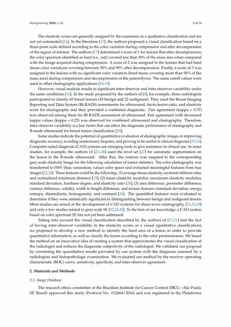
The elasticity scores are generally assigned by the examiners as a qualitative classification and arenot yet automated [16]. In the literature [17], the authors proposed a visual classification based on athree-point scale defined according to the color variation during compression and after decompressionof the region of interest. The authors [17] determined a score of 1 for lesions that after decompression,the color spectrum identified as hard (i.e., red) covered less than 50% of the mass area when comparedwith the image acquired during compression. A score of 2 was assigned to the lesions that had hardtissue color variations covering between 50% and 90% after decompression. Finally, a score of 3 wasassigned to the lesions with no significant color variation (hard tissue covering more than 90% of themass area) during compression and decompression of the parenchyma. The same cutoff values wereused in other elastography applications [18,19].

However, visual analysis results in significant inter-observer and intra-observer variability underthe same conditions [16]. In the study proposed by the authors of [8], for example, three radiologistsparticipated to classify 65 breast lesions (43 benign and 22 malignant). They used the Breast ImagingReporting and Data System (BI-RADS) assessments for ultrasound, fat-to-lesion ratio, and elasticityscore for elastography and they provided a combined diagnostic. Fair agreement (kappa = 0.37)was observed among them for BI-RADS assessment of ultrasound. Fair agreement with decreasedkappa values (kappa = 0.25) was observed for combined ultrasound and elastography. Therefore,inter-observer variability is a key factor that can affect the diagnostic performance of elastography andB-mode ultrasound for breast tumor classification [20].

Some studies indicate the potential of quantitative evaluation of elastographic images in improvingdiagnostic accuracy, avoiding unnecessary biopsies, and proving to be useful in clinical diagnosis [15,16].Computer-aided diagnosis (CAD) systems are emerging tools to give assistance in clinical use. In somestudies, for example, the authors of [21–26] used the level set [27] for automatic segmentation onthe lesion in the B-mode ultrasound. After that, the contour was mapped to the correspondinggrey-scale elasticity image for the following calculation of tumor statistics. The color elastography wastransferred to HSV (hue, saturation, value) color space and extracted meaningful features from hueimages [23,28]. These features could be the following: (1) average tissue elasticity, sectional stiffness ratio,and normalized minimum distance [23]; (2) mean elasticity modulus, maximum elasticity modulus,standard deviation, hardness degree, and elasticity ratio [29]; (3) area difference, perimeter difference,contour difference, solidity, width to height difference, and texture features (standard deviation, energy,entropy, dissimilarity, homogeneity, and contrast) [30]. The quantified features were evaluated todetermine if they were statistically significant in distinguishing between benign and malignant lesions.Most studies are aimed at the development of CAD systems for shear-wave eslatography [21,23,29]and only a few studies related to gray-scale SE [22,24,28]. To the best of our knowledge, a CAD systembased on color spectrum SE has not yet been addressed.

Taking into account the visual classification described by the authors of [17,31] and the factof having inter-observer variability in the elasticity scores as a visual (qualitative classification),we proposed to develop a new method to identify the hard area of a lesion in order to providequantitative information, as well as classify the lesion according to the color predominance. We basedthe method on an innovative idea of creating a system that approximates the visual classification ofthe radiologist and reduces the diagnostic subjectivity of the radiologist. We validated our proposalby correlating the quantitative results provided by our system with the diagnosis assessed by aradiologists and histopathologic examination. We evaluated our method by the receiver operatingcharacteristic (ROC) curve, sensitivity, specificity, and inter-observer agreement.

2. Materials and Methods

2.1. Image Database

The research ethics committee of the Brazilian Institute for Cancer Control (IBCC—São Paulo,SP, Brazil) approved this study (Protocol No. 012664/2016) and was registered in the Plataforma

Bioengineering 2018, 5, 62 4 of 14

Brazil (Protocol No. 53543016.2.0000.0072). Investigators of the study obtained written informedconsent from all included patients and protected their privacy. The collection of cases was from Julyto December 2015 during diagnostic breast exams at the IBCC. The data consisted of 83 consecutivewomen, represented by 92 solid lesions. All lesions underwent excisional biopsy; core needle biopsy;or fine-needle aspiration biopsy for pathologic diagnosis, used as the gold standard for evaluation ofthe CAD system. However, five patients were excluded because they presented non-mass lesions onthe ultrasound before the percutaneous biopsy confirmation. A total of 83 lesions were included in thestudy, resulting in 31 malignant and 52 benign lesions.

The mean age of the patients submitted to the study was 46.5 years, ranging from 23 to 73 years(standard deviation of 8.6). The mean lesion size was 11 mm (ranging from 2.39 to 28.3 mm).Positive results for carcinoma were found in 6 patients younger than 40 years (19.3%), 11 patientsbetween 40 and 50 years old (35.5%), and 14 patients older than 50 years (45.2%).

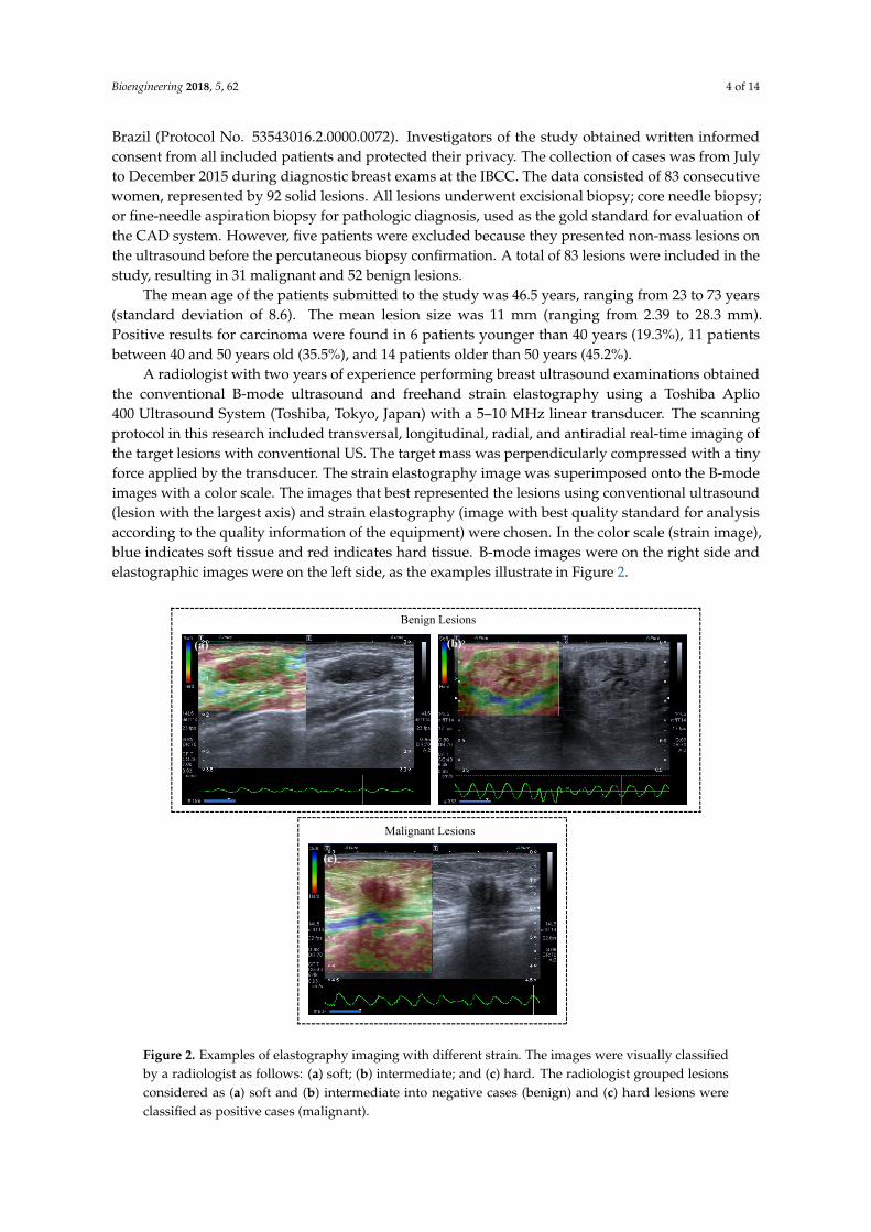
A radiologist with two years of experience performing breast ultrasound examinations obtainedthe conventional B-mode ultrasound and freehand strain elastography using a Toshiba Aplio400 Ultrasound System (Toshiba, Tokyo, Japan) with a 5–10 MHz linear transducer. The scanningprotocol in this research included transversal, longitudinal, radial, and antiradial real-time imaging ofthe target lesions with conventional US. The target mass was perpendicularly compressed with a tinyforce applied by the transducer. The strain elastography image was superimposed onto the B-modeimages with a color scale. The images that best represented the lesions using conventional ultrasound(lesion with the largest axis) and strain elastography (image with best quality standard for analysisaccording to the quality information of the equipment) were chosen. In the color scale (strain image),blue indicates soft tissue and red indicates hard tissue. B-mode images were on the right side andelastographic images were on the left side, as the examples illustrate in Figure 2.

Bioengineering 2018, 5, x FOR PEER REVIEW 4 of 13

to December 2015 during diagnostic breast exams at the IBCC. The data consisted of 83 consecutive

women, represented by 92 solid lesions. All lesions underwent excisional biopsy; core needle biopsy;

or fine-needle aspiration biopsy for pathologic diagnosis, used as the gold standard for evaluation of

the CAD system. However, five patients were excluded because they presented non-mass lesions on

the ultrasound before the percutaneous biopsy confirmation. A total of 83 lesions were included in

the study, resulting in 31 malignant and 52 benign lesions.

The mean age of the patients submitted to the study was 46.5 years, ranging from 23 to 73 years

(standard deviation of 8.6). The mean lesion size was 11 mm (ranging from 2.39 to 28.3 mm). Positive

results for carcinoma were found in 6 patients younger than 40 years (19.3%), 11 patients between 40

and 50 years old (35.5%), and 14 patients older than 50 years (45.2%).

A radiologist with two years of experience performing breast ultrasound examinations obtained

the conventional B-mode ultrasound and freehand strain elastography using a Toshiba Aplio 400

Ultrasound System (Toshiba, Tokyo, Japan) with a 5–10 MHz linear transducer. The scanning

protocol in this research included transversal, longitudinal, radial, and antiradial real-time imaging

of the target lesions with conventional US. The target mass was perpendicularly compressed with a

tiny force applied by the transducer. The strain elastography image was superimposed onto the B-

mode images with a color scale. The images that best represented the lesions using conventional

ultrasound (lesion with the largest axis) and strain elastography (image with best quality standard

for analysis according to the quality information of the equipment) were chosen. In the color scale

(strain image), blue indicates soft tissue and red indicates hard tissue. B-mode images were on the

right side and elastographic images were on the left side, as the examples illustrate in Figure 2.

Figure 2. Examples of elastography imaging with different strain. The images were visually classified

by a radiologist as follows: (a) soft; (b) intermediate; and (c) hard. The radiologist grouped lesions

considered as (a) soft and (b) intermediate into negative cases (benign) and (c) hard lesions were

classified as positive cases (malignant).

Benign Lesions

Malignant Lesions

(a) (b)

(c)

Figure 2. Examples of elastography imaging with different strain. The images were visually classifiedby a radiologist as follows: (a) soft; (b) intermediate; and (c) hard. The radiologist grouped lesionsconsidered as (a) soft and (b) intermediate into negative cases (benign) and (c) hard lesions wereclassified as positive cases (malignant).

Bioengineering 2018, 5, 62 5 of 14

2.2. Delimitation of the Lesion

In elasticity imaging, automatic segmentation of lesions is a difficult task because of thedistribution of colors, irregularity of the image, and difficulty in the direct extraction of the lesioncontour [28]. Therefore, it was opted for the three radiologists to manually and arbitrarily delineatethe contour of the lesions in the B-mode ultrasound images [28,29]. After manual delimitation of themass on the B-mode image, the extracted tumor was masked to the corresponding elasticity image forthe calculation of the hard area in the lesion.

2.3. Classification

In order to measure the amount of hard tissue (i.e., tissues in red) in a lesion, we developed analgorithm for segmenting red areas and quantifying its predominance within the lesion, allowing us toclassify it as soft, intermediate, or hard. The developed system is the result of an automatic process,in which the variable is the manual delimitation of the contour by the radiologist. The CAD systemflowchart is presented in Figure 3. We compared the automatic classification with the percutaneousbiopsy results.

Bioengineering 2018, 5, x FOR PEER REVIEW 5 of 13

2.2. Delimitation of the Lesion

In elasticity imaging, automatic segmentation of lesions is a difficult task because of the

distribution of colors, irregularity of the image, and difficulty in the direct extraction of the lesion

contour [28]. Therefore, it was opted for the three radiologists to manually and arbitrarily delineate

the contour of the lesions in the B-mode ultrasound images [28,29]. After manual delimitation of the

mass on the B-mode image, the extracted tumor was masked to the corresponding elasticity image

for the calculation of the hard area in the lesion.

2.3. Classification

In order to measure the amount of hard tissue (i.e., tissues in red) in a lesion, we developed an

algorithm for segmenting red areas and quantifying its predominance within the lesion, allowing us

to classify it as soft, intermediate, or hard. The developed system is the result of an automatic process,

in which the variable is the manual delimitation of the contour by the radiologist. The CAD system

flowchart is presented in Figure 3. We compared the automatic classification with the percutaneous

biopsy results.

Figure 3. Computer-aided diagnosis system for breast tumor classification.

A color model is a mathematical way of representing colors in numbers. There are several

models and each one was derived for specific purposes and has certain advantages over the others.

The main disadvantage of the RGB (red, green, blue) color space is related to the difficulty of

recognizing different levels of intensity of the same chrominance. To avoid light intensity influence,

we used the CIELab color space (also called L*a*b*) [32,33]. CIELab is a color space defined by the

International Commission on Illumination (CIE) to express the color as three numerical values. It is

represented by three matrices: brightness, green-red, and blue-yellow. The color axes are based on

the fact that a color cannot be red and green or blue and yellow, because these colors oppose each

other. On each axis, the values run from positive to negative (ranges from −127 to +127). On the a*

axis, positive values indicate amounts of red, while negative values indicate amounts of green. On

the b* axis, yellow is positive and blue is negative. The lightness or gray-scale axis (L*) represents the

darkest black (L* = 0) and the brightest white (L* = 100). The asterisk (*) after L, a, and b are part of

the full name to distinguish them from Hunter’s Lab color space [32,33]. Figure 4 illustrates an

example of a fibroadenoma with the color channels from RGB and CIELab color space displayed

Figure 3. Computer-aided diagnosis system for breast tumor classification.

A color model is a mathematical way of representing colors in numbers. There are several modelsand each one was derived for specific purposes and has certain advantages over the others. The maindisadvantage of the RGB (red, green, blue) color space is related to the difficulty of recognizing differentlevels of intensity of the same chrominance. To avoid light intensity influence, we used the CIELab colorspace (also called L*a*b*) [32,33]. CIELab is a color space defined by the International Commission onIllumination (CIE) to express the color as three numerical values. It is represented by three matrices:brightness, green-red, and blue-yellow. The color axes are based on the fact that a color cannot be redand green or blue and yellow, because these colors oppose each other. On each axis, the values runfrom positive to negative (ranges from −127 to +127). On the a* axis, positive values indicate amountsof red, while negative values indicate amounts of green. On the b* axis, yellow is positive and blue isnegative. The lightness or gray-scale axis (L*) represents the darkest black (L* = 0) and the brightestwhite (L* = 100). The asterisk (*) after L, a, and b are part of the full name to distinguish them fromHunter’s Lab color space [32,33]. Figure 4 illustrates an example of a fibroadenoma with the color

Bioengineering 2018, 5, 62 6 of 14

channels from RGB and CIELab color space displayed separately. The contour was manually drawnby the radiologist and the adjacent tissues were removed from the image to improve the visualizationof the mass.

Bioengineering 2018, 5, x FOR PEER REVIEW 6 of 13

separately. The contour was manually drawn by the radiologist and the adjacent tissues were

removed from the image to improve the visualization of the mass.

Analyzing the a* channel, we noted that it is possible to easily identify the red color, as it is

represented by the lighter pixels. For this procedure, the Otsu method was applied [34] on the a*

channel. The Otsu method is used to automatically perform clustering-based image thresholding or

the reduction of a gray level image to a binary image. The algorithm assumes that the image contains

two classes of pixels following bi-modal histogram (foreground pixels and background pixels), it then

calculates the optimum threshold separating the two classes so that their combined spread (intra-

class variance) is minimal, or equivalently (because the sum of pairwise squared distances is

constant), so that their inter-class variance is maximal.

Figure 4. RGB and CIELab color space with their color channels shown separately.

The cut-off point of classification is based on the percentage value of hard tissue in relation to

the total area of the lesion. In order to find the best value of separation between benign and malignant

lesions, we evaluated the performance of the CAD system using four values for the cut-off point.

Table 1 shows the AUC obtained in each cut-off point.

Table 1. Classification with different cut-off point. AUC—area under the curve.

Observers AUC—70% of

Hard Tissue

AUC—75% of

Hard Tissue

AUC—80% of

Hard Tissue

AUC—90% of

Hard Tissue

Radiologist 1 0.841 0.853 0.802 0.790

Radiologist 2 0.813 0.806 0.815 0.707

Resident 0.802 0.814 0.789 0.723

Visual Analysis—Radiologist 1 0.829

Radiologist 1 performed a prior visual analysis of the lesions, and after six months with no eye

contact with the images, he manually delimited the contour of the lesions. Data from the visual

Figure 4. RGB and CIELab color space with their color channels shown separately.

Analyzing the a* channel, we noted that it is possible to easily identify the red color, as it isrepresented by the lighter pixels. For this procedure, the Otsu method was applied [34] on the a*channel. The Otsu method is used to automatically perform clustering-based image thresholding orthe reduction of a gray level image to a binary image. The algorithm assumes that the image containstwo classes of pixels following bi-modal histogram (foreground pixels and background pixels), it thencalculates the optimum threshold separating the two classes so that their combined spread (intra-classvariance) is minimal, or equivalently (because the sum of pairwise squared distances is constant),so that their inter-class variance is maximal.

The cut-off point of classification is based on the percentage value of hard tissue in relation to thetotal area of the lesion. In order to find the best value of separation between benign and malignantlesions, we evaluated the performance of the CAD system using four values for the cut-off point.Table 1 shows the AUC obtained in each cut-off point.

Table 1. Classification with different cut-off point. AUC—area under the curve.

Observers AUC—70% ofHard Tissue

AUC—75% ofHard Tissue

AUC—80% ofHard Tissue

AUC—90% ofHard Tissue

Radiologist 1 0.841 0.853 0.802 0.790Radiologist 2 0.813 0.806 0.815 0.707

Resident 0.802 0.814 0.789 0.723

Visual Analysis—Radiologist 1 0.829

Bioengineering 2018, 5, 62 7 of 14

Radiologist 1 performed a prior visual analysis of the lesions, and after six months with no eyecontact with the images, he manually delimited the contour of the lesions. Data from the visual analysisare related to the clinical diagnosis provided by Radiologist 1, who did not use the computationalsystem to assist in his diagnosis. However, Radiologist 1 was the only one who performed thevisual analysis.

The best cut-off point achieved was 75% of hard lesions because it provided better AUC for twoof the three classification tests, in which one of them was using the delimitation of the contour by themost experienced radiologist.

After finding the cut-off point that would provide the best distinction between benign andmalignant lesions, the lesion was classified as follows: (1) soft for lesions with red areas lower than50% of the total area delineated by the observers; (2) intermediate for lesions with red areas between50–75%; and (3) hard for red areas higher than 75% of the total lesion area. From the redefinitionof classification values that had initially been proposed by the authors of [17], we achieved betterdiagnostic accuracy for this threshold values, as shown in previous work [35]. We considered lesionsclassified as soft and intermediate to be benign and hard to be malignant.

As output, the system provides two images: an image with the region classified as hard (redregion) and another image with the region classified as soft (other colors). Thus, the radiologist cananalyze the reliability of the computational diagnosis. Furthermore, the system also provides thepercentage value of hard tissue in the lesion, representing the tendency of malignancy, in which 0%corresponds to benign lesions and 100% to malignant lesions, as shown in Figure 5.

Bioengineering 2018, 5, x FOR PEER REVIEW 7 of 13

analysis are related to the clinical diagnosis provided by Radiologist 1, who did not use the

computational system to assist in his diagnosis. However, Radiologist 1 was the only one who

performed the visual analysis.

The best cut-off point achieved was 75% of hard lesions because it provided better AUC for two

of the three classification tests, in which one of them was using the delimitation of the contour by the

most experienced radiologist.

After finding the cut-off point that would provide the best distinction between benign and

malignant lesions, the lesion was classified as follows: (1) soft for lesions with red areas lower than

50% of the total area delineated by the observers; (2) intermediate for lesions with red areas between

50–75%; and (3) hard for red areas higher than 75% of the total lesion area. From the redefinition of

classification values that had initially been proposed by the authors of [17], we achieved better

diagnostic accuracy for this threshold values, as shown in previous work [35]. We considered lesions

classified as soft and intermediate to be benign and hard to be malignant.

As output, the system provides two images: an image with the region classified as hard (red

region) and another image with the region classified as soft (other colors). Thus, the radiologist can

analyze the reliability of the computational diagnosis. Furthermore, the system also provides the

percentage value of hard tissue in the lesion, representing the tendency of malignancy, in which 0%

corresponds to benign lesions and 100% to malignant lesions, as shown in Figure 5.

Figure 5. Classification using the system proposed.

2.4. Data Evaluation and Statistical Analysis

Two radiologists, with 16 and 10 years of experience, and a second-year resident in imaging

diagnosis, drew the contour of the lesions and assisted in evaluating our algorithm.

We compared the manual delimitation of the observers using the following measures: the Jaccard

Similarity Index (JSI) [36], oversegmentation (AVM) [37], and undersegmentation (AUM) [37].

JSI was used to compare the similarity of a data set, and was defined by the ratio between the

intersection and the union of two areas (Equation (1)).

JSI =���� ∩ ���

���� ∪ ���

(1)

where ���� denotes the segmented area and ��� is the corresponding ground truth area. JSI ranges

from 0 to 1, and the higher the value, the better the segmentation result.

Jaccard does not provide information on the undersegmentation and oversegmentation. So,

AUM and AVM were measured and are defined by Equations (2) and (3).

AUM = ��� − ����

���

(2)

AVM = ���� − ���

����

(3)

Figure 5. Classification using the system proposed.

2.4. Data Evaluation and Statistical Analysis

Two radiologists, with 16 and 10 years of experience, and a second-year resident in imagingdiagnosis, drew the contour of the lesions and assisted in evaluating our algorithm.

We compared the manual delimitation of the observers using the following measures: the JaccardSimilarity Index (JSI) [36], oversegmentation (AVM) [37], and undersegmentation (AUM) [37].

JSI was used to compare the similarity of a data set, and was defined by the ratio between theintersection and the union of two areas (Equation (1)).

JSI =Aseg ∩ Agt

Aseg ∪ Agt(1)

where Aseg denotes the segmented area and Agt is the corresponding ground truth area. JSI rangesfrom 0 to 1, and the higher the value, the better the segmentation result.

Jaccard does not provide information on the undersegmentation and oversegmentation. So,AUM and AVM were measured and are defined by Equations (2) and (3).

AUM =Agt − Aseg

Agt(2)

Bioengineering 2018, 5, 62 8 of 14

AVM =Aseg − Agt

Aseg(3)

Values of AUM and AVM range from 0 to 1, and large values indicate undersegmentation oroversegmentation, respectively.

The kappa coefficient [38] was used to measure the inter-rater agreement, in which 0.0–0.2 wasconsidered poor, 0.21–0.40 fair, 0.41–0.60 moderate, 0.61–0.80 good, and 0.81–1.00 very good agreement.We calculated the sensitivity, specificity, and ROC curves for all the observers. The ROC curves wereobtained using bootstrapping with 95% confidence intervals (CI) in all cases and were compared usinga significance level of 5%. For the calculation of the kappa coefficient, sensitivity, specificity, and AUC,we used the Med Calc software v16.2 (MedCalc Software, Ostend, Belgium), with significant levels atp < 0.05.

3. Results

3.1. Manual Delineation

Figure 6 illustrates the manual delimitation of the lesion on the B-mode ultrasound and thesuperposition of the contour in the elastography image.

Bioengineering 2018, 5, x FOR PEER REVIEW 8 of 13

Values of AUM and AVM range from 0 to 1, and large values indicate undersegmentation or

oversegmentation, respectively.

The kappa coefficient [38] was used to measure the inter-rater agreement, in which 0.0–0.2 was

considered poor, 0.21–0.40 fair, 0.41–0.60 moderate, 0.61–0.80 good, and 0.81–1.00 very good

agreement. We calculated the sensitivity, specificity, and ROC curves for all the observers. The ROC

curves were obtained using bootstrapping with 95% confidence intervals (CI) in all cases and were

compared using a significance level of 5%. For the calculation of the kappa coefficient, sensitivity,

specificity, and AUC, we used the Med Calc software v16.2 (MedCalc Software, Ostend, Belgium),

with significant levels at p < 0.05.

3. Results

3.1. Manual Delineation

Figure 6 illustrates the manual delimitation of the lesion on the B-mode ultrasound and the

superposition of the contour in the elastography image.

Figure 6. Results of the manual delineation of the tumor on B-mode image and contour mapped on

the elasticity image.

The radiologists were blinded to the diagnosis when they manually delimited the contour of the

lesion. Table 2 gives the agreement between the three radiologists’ manual delineation, using

different measures.

Table 2. Measures to evaluate the manual delineation.

Observers Jaccard Undersegmentation Oversegmentation

Radiologist 1 and Radiologist 2 Average 0.565 0.147 0.355

SD 0.178 0.144 0.213

Radiologist 1 and Resident Average 0.654 0.227 0.169

SD 0.122 0.148 0.135

Radiologist 2 and Resident Average 0.537 0.402 0.144

SD 0.193 0.212 0.174

Mean Value Desired 1.000 0.000 0.000

The desired value corresponds to the perfect overlap (JSI = 1.0) between the considered

segmented areas, with neither oversegmentation (AVM = 0) nor undersegmentation (AUM = 0).

The highest conformity in manual delineation occurred between Radiologist 1 and the Resident,

wherein they obtained the highest overlap index (JSI of 0.654) and low indices of undersegmentation

Figure 6. Results of the manual delineation of the tumor on B-mode image and contour mapped on theelasticity image.

The radiologists were blinded to the diagnosis when they manually delimited the contourof the lesion. Table 2 gives the agreement between the three radiologists’ manual delineation,using different measures.

Table 2. Measures to evaluate the manual delineation.

Observers Jaccard Undersegmentation Oversegmentation

Radiologist 1 and Radiologist 2 Average 0.565 0.147 0.355SD 0.178 0.144 0.213

Radiologist 1 and Resident Average 0.654 0.227 0.169SD 0.122 0.148 0.135

Radiologist 2 and Resident Average 0.537 0.402 0.144SD 0.193 0.212 0.174

Mean Value Desired 1.000 0.000 0.000

Bioengineering 2018, 5, 62 9 of 14

The desired value corresponds to the perfect overlap (JSI = 1.0) between the considered segmentedareas, with neither oversegmentation (AVM = 0) nor undersegmentation (AUM = 0).

The highest conformity in manual delineation occurred between Radiologist 1 and the Resident,wherein they obtained the highest overlap index (JSI of 0.654) and low indices of undersegmentationand oversegmentation (0.227 and 0.169, respectively). On the other hand, the lowest conformity wasbetween Radiologist 2 and the Resident, considering mainly the high index of undersegmentation(0.402) of the Resident in relation with Radiologist 2. Values are expressed in more detail in Table 2.

3.2. Classification Evaluation

We used the sensitivity, specificity, and the area under the ROC curve (AUC) measure to evaluatethe performance of the CAD system with the contour delineated by each specialist. Table 3 shows theresults of the classification using the cut-off of 75%.

Table 3. Classification of the lesions based on the manual delimitation of radiologists.

Observers Sensitivity Specificity AUC

Radiologist 1 70.97 88.46 0.853Radiologist 2 67.74 84.62 0.806

Resident 58.06 90.38 0.814Visual Analysis—Radiologist 1 61.29 88.46 0.829

Table 4 shows the final classification of the lesions using the CAD system from the contourdelineated of each radiologist according to the histological diagnosis (benign or malignant).

Table 4. Distribution of the final classification according to the score adopted, where score 1 representssoft lesions; score 2 represents intermediate; and score 3 is associated with hard lesions.

Type nRadiologist 1 Radiologist 2 Resident

Median Mean Median Mean Median Mean

Benign(n = 48)

Fibrocystic changes 30 2.0 1.7 1.0 1.7 1.5 1.7Fibroadenoma 18 2.0 1.6 2.0 1.6 2.0 1.6

Malignant(n = 31)

Invasive ductal carcinoma 23 3.0 2.5 3.0 2.5 3.0 2.4Invasive lobular carcinoma 2 3.0 3.0 3.0 3.0 3.0 3.0

Ductal Carcinoma in Situ (DCIS) 4 3.0 3.0 2.5 2.5 2.5 2.5Others 2 2.5 2.5 2.5 2.5 2.5 2.5

Indeterminate(n = 4) Indeterminate lesions 4 2.0 1.8 2.0 2.3 2.0 2.0

Total 83 -

The mean and median values correspond to the classification score. Score 1 was assigned to softlesions, score 2 to intermediate lesions, and score 3 to hard lesions.

3.3. Statistics Analysis

Table 5 shows the inter-observer agreement (kappa coefficient) for all the observers. The intra-classcorrelation coefficient was 0.748.

Table 5. Inter-observer agreement in the diagnosis of lesions in elastography imaging using thecomputer-aided diagnosis (CAD) system with different contours.

Observers Kappa

Radiologist 1 and Radiologist 2 0.796Radiologist 1 and Resident 0.758Radiologist 2 and Resident 0.682

Bioengineering 2018, 5, 62 10 of 14

We used the kappa coefficient to evaluate the concordance in the diagnosis of the CAD systemwith the contour of the lesion performed by specialists with different levels of experience in order toverify the susceptibility of our system to the contour. Based on the results presented in the table above,the agreement was good in all cases. The best agreement was found in the comparison between theCAD system with the contours of Radiologists 1 and 2.

Table 6 compares the differences in AUC values between all the radiologists, considering the visualanalysis provided by Radiologist 1 and the automatic classification based on the manual delineation ofeach one.

Table 6. Classification based on automatic system.

Observers Difference in AUC 95% Confidence Intervals (CI) p-Value

Visual Analysis—Radiologist 1 0.024 −0.048–0.096 0.517Visual Analysis—Radiologist 2 0.023 −0.050–0.096 0.538

Visual Analysis—Resident 0.033 −0.047–0.113 0.420

Radiologist 1 and Radiologist 2 0.047 −0.024–0.118 0.196Radiologist 1 and Resident 0.057 −0.015–0.128 0.120Radiologist 2 and Resident 0.010 −0.081–0.101 0.830

The table above shows that there is practically no inter-observer variation in the AUC. Althoughslight, the greatest variation is noted in the comparison between Radiologist 1 and Resident. This isbecause of the difference in experience time between them.

4. Discussion

The American College of Radiology suggests elasticity assessment as a way to evaluate breasttumor malignancy in the fifth edition of Breast Imaging Reporting and Data System (BI-RADS),released in 2013 [39]. The suggestion indicates that elastography provides additional diagnosticinformation over conventional B-mode imaging. This is in order to improve differentiation of benignand malignant breast tumors and avoid unnecessary biopsy.

The analysis of strain images involves the evaluation of the distribution of colors within thelesion and allows the classification of these lesions as soft, intermediate, or hard, as proposed by theBI-RADS lexicon. The inter-observer agreement is uncertain in the strain method because it is operatordependent and the results are qualitative.

This study presented a CAD system based on SE elastography images that could enable objectiveevaluation of the hard tissues of breast masses. The CAD system proposed is an innovative methodthat attempts to classify the lesion in a similar way to the specialist’s visual classification and providesquantitative information regarding the hard tissues present within the lesion.

In a CAD system, the accurate segmentation of breast lesions in US images is a difficult task,mainly in automatic systems, as a result of presence of speckle noise and shadows, the low ornon-uniform contrast of certain structures, and the variability of the echogenicity of the masses,while manual delineation is a subjective, time-consuming, and operator-dependent procedure.

We performed an initial study to evaluate the manual segmentation of the radiologists,because errors or distortions in the lesion representation may result in misdiagnosis. In our study,Resident (less experienced observer) presented manual delineation closer to Radiologist 1 (the mostexperienced), with a higher Jaccard index (0.654) and lower oversegmentation (0.169). When wemeasured inter-observer agreement, the observers obtained a good value (kappa = 0.758). On the otherhand, Radiologist 2 did not produce manual delineation as close to Radiologist 1 as that of Resident,with a similar inter-observer agreement (kappa = 0.796). We consider that the change in contour wasnot a harmful factor in the classification.

The computer method was compared with the physician’s visual diagnosis. The system providedan increase in sensitivity (70.97% vs. 61.29%) and the specificity remained constant (88.46%),

Bioengineering 2018, 5, 62 11 of 14

compared with the visual assessment by Radiologist 1 (see Table 3). The AUC value was 0.853 for thecase using the new method by computer, and 0.829 for the visual assessment. In relation to Radiologist2 and Resident, they reached AUCs of 0.806 and 0.814, respectively. Furthermore, we achieved goodagreement among all observers, indicating that the CAD system can aid in the interpretation of theelastography image.

This research is an apparent improvement of a previous work [35], in which we developedanother color classification approach. The previous system was more user-dependent and presentedsignificant inter- and intra-observer variation. This is because the user had to manually delimit a partof the red region, which may affect classifying the lesion. Based on the exposed, the algorithm hadalready presented results [35] comparable to the visual classification of the radiologist with sensitivity,specificity, and an AUC value of 54.5%, 90.5%, and 0.837, respectively.

In the study proposed by Chang [28], they evaluated the performance of a new computer-aidedmethod on color strain elastography in the differentiation of benign and malignant breast lesions.Their method consisted of the conversion from RGB to HSV color space and the extraction of six features(tumor mean, inner mean, outer mean, hard rate, inner hard, and outer hard) from hue images. Then,the neural network was utilized to distinguish tumors. The proposed CAD system presented betterperformance than the physician with 85.07% of sensitivity and 83.19% of specificity in comparisonwith 53.73% of sensitivity and 92.92% specificity from the physician. The kappa statistics was appliedto measure the agreement between the proposed CAD system and the physician’s diagnosis, the kappaof 0.54 indicated the moderate agreement between observers. Lo [22] presented an approach of CADsystem for gray-scale strain elastography. They extracted the contour using pre-processing techniquesfor contrast enhancement and level set to detect the edge of the lesion. The fuzzy c-means methodwas used to classify the pixels into three clusters and define the stiff area. Six strain features wereextracted and the leave-one-out cross-validation method was used to validate the performance of theselected subset. As a result, the diagnostic performance of the CAD system achieved values of 80%,80%, and 0.84 for sensitivity, specificity, and AUC, respectively.

One factor to consider is the lack of a public breast elastography image database. As theperformance of the algorithms is dependent on the images that are collected for each work, resultscannot be reliably compared.

The limitations of this study include the fact that the entire dataset was used in the trainingprocess and the lack of an automatic segmentation method. Another limitation is that the proposedsystem is based on the detection and quantification of the red color, whose prevalence determines thedegree of stiffness of a lesion. A possible improvement of the CAD system could be the inclusion ofthe B-mode features, such as those related to the morphology and texture of the lesion, in addition tothe use of machine learning techniques. On the other hand, the system is simple, fast, and achievessimilar or better results among the mentioned works, proving to be an important tool for classifyingbreast lesions in elastography images.

5. Conclusions

The proposed CAD system can reduce the inter-observer variability for breast elastography.The CAD system had a similar performance to the diagnosis of the most experienced radiologist,which would provide promising diagnoses in clinical use. In future work, we intend to evaluate thevisual analysis of more radiologists, in order to include automatic segmentation techniques, as wellas to include more features and study other types of automatic classifiers, such as machine learningtechniques. In addition, an ultrasound image characterization system could be included in our CADsystem in order to provide more information about the lesion, increasing the diagnostic accuracy inclassifying breast elastography images.

Bioengineering 2018, 5, 62 12 of 14

Author Contributions: Formal analysis, K.D.M.; Methodology, K.D.M.; Project administration, H.S.; Software,K.D.M.; Supervision, E.F.C.F., V.M.O., A.A.O.C., H.S. and R.M.N.; Validation, E.F.C.F.; Writing—original draft,K.D.M.; Writing—review & editing, E.F.C.F. and R.M.N.

Funding: This work was supported by the São Paulo Research Foundation (FAPESP) grant #2012/24006-5 andgrant #2015/17302-5.

Acknowledgments: To FAPESP for the financial support.

Conflicts of Interest: The authors declare no conflict of interest. The content is solely the responsibility of theauthors and does not necessarily represent the official views of FAPESP.

References

1. Shan, J.; Alam, S.K.; Garra, B.; Zhang, Y.; Ahmed, T. Computer-Aided Diagnosis for Breast Ultrasound UsingComputerized BI-RADS Features and Machine Learning Methods. Ultrasound Med. Biol. 2016, 42, 980–988.[CrossRef] [PubMed]

2. Ricci, P.; Maggini, E.; Mancuso, E.; Lodise, P.; Cantisani, V.; Catalano, C. Clinical application of breastelastography: State of the art. Eur. J. Radiol. 2014, 83, 429–437. [CrossRef] [PubMed]

3. Huang, Q.; Luo, Y.; Zhang, Q. Breast ultrasound image segmentation: A survey. Int. J. Comput. Assist.Radiol. Surg. 2017, 12, 493–507. [CrossRef] [PubMed]

4. Ekeh, A.P.; Alleyne, R.S.; Duncan, A.O. Role of mammography in diagnosis of breast cancer in an inner-cityhospital. J. Natl. Med. Assoc. 2000, 92, 372–374. [PubMed]

5. Stavros, A.T.; Thickman, D.; Rapp, C.L.; Dennis, M.A.; Parker, S.H.; Sisney, G.A. Solid breast nodules: Use ofsonography to distinguish between benign and malignant lesions. Radiology 1995, 196, 123–134. [CrossRef][PubMed]

6. Lu, R.; Xiao, Y.; Liu, M.; Shi, D. Ultrasound elastography in the differential diagnosis of benign and malignantcervical lesions. J. Ultrasound Med. 2014, 33, 667–671. [CrossRef] [PubMed]

7. Awad, F.M. Role of supersonic shear wave imaging quantitative elastography (SSI) in differentiating benignand malignant solid breast masses. Egypt. J. Radiol. Nucl. Med. 2013, 44, 681–685. [CrossRef]

8. Yoon, J.H.; Kim, M.H.; Kim, E.-K.; Moon, H.J.; Kwak, J.Y.; Kim, M.J. Interobserver Variability of UltrasoundElastography: How It Affects the Diagnosis of Breast Lesions. Am. J. Roentgenol. 2011, 196, 730–736.[CrossRef] [PubMed]

9. Barr, R.G. Breast Elastography; Thieme Medical: New York, NY, USA, 2015.10. Balleyguier, C.; Canale, S.; Hassen, W.B.; Vielh, P.; Bayou, E.H.; Mathieu, M.C.; Uzan, C.; Bourgier, C.;

Dromain, C. Breast elasticity: Principles, technique, results: An update and overview of commerciallyavailable software. Eur. J. Radiol. 2013, 82, 427–434. [CrossRef] [PubMed]

11. Zippel, D.; Shalmon, A.; Rundstein, A.; Novikov, I.; Yosepovich, A.; Zbar, A.; Goitein, D.; Sklair-Levy, M.Freehand Elastography for Determination of Breast Cancer Size: Comparison With B-Mode Sonography andHistopathologic Measurement. J. Ultrasound Med. 2014, 33, 1441–1446. [CrossRef] [PubMed]

12. Ophir, J. Elastography: A quantitative method for imaging the elasticity of biological tissues.Ultrason. Imaging 1991, 13, 111–134. [CrossRef] [PubMed]

13. Hall, T. In vivo real-time freehand palpation imaging. Ultrasound Med. Biol. 2003, 29, 427–435. [CrossRef]14. Diaz, J.J.; Castellanos, N.P.; Pineda, C.; Hernandez, C.; Ventura, L.; Gutierrez, J. Algorithm to estimate the

level of elasticity of biological tissue with ultrasound elastography images. In Proceedings of the 2015 PanAmerican Health Care Exchanges (PAHCE), Vina del Mar, Chile, 23–28 March 2015. [CrossRef]

15. Zhi, H.; Xiao, X.Y.; Yang, H.Y.; Wen, Y.L.; Ou, B.; Luo, B.M.; Liang, B.L. Semi-quantitating Stiffness of BreastSolid Lesions in Ultrasonic Elastography. Acad. Radiol. 2008, 15, 1347–1353. [CrossRef] [PubMed]

16. Zhang, X.; Xiao, Y.; Zeng, J.; Qiu, W.; Qian, M.; Wang, C.; Zheng, R.; Zheng, H. Computer-assisted assessmentof ultrasound real-time elastography: Initial experience in 145 breast lesions. Eur. J. Radiol. 2014, 83, 1–7.[CrossRef] [PubMed]

17. Fleury, E.F.C. The importance of breast elastography added to the BI-RADS(R) (5th edition) lexiconclassification. Assoc. Med. Bras. 2015, 61, 313–316. [CrossRef] [PubMed]

18. Lo, W.C.; Cheng, P.W.; Wang, C.T.; Liao, L.J. Real-time ultrasound elastography: An assessment of enlargedcervical lymph nodes. Eur. Radiol. 2013, 23, 2351–2357. [CrossRef] [PubMed]

Bioengineering 2018, 5, 62 13 of 14

19. Choi, Y.J.; Lee, J.H.; Baek, J.H. Ultrasound elastography for evaluation of cervical lymph nodes.Ultrasonography 2015, 34, 157–164. [CrossRef] [PubMed]

20. Moon, W.K.; Chang, S.C.; Chang, J.M.; Cho, N.; Huang, C.S.; Kuo, J.W.; Chang, R.F. Classification of BreastTumors Using Elastographic and B-mode Features: Comparison of Automatic Selection of RepresentativeSlice and Physician-Selected Slice of Images. Ultrasound Med. Biol. 2013, 39, 1147–1157. [CrossRef] [PubMed]

21. Xiao, Y.; Zeng, J.; Qian, M.; Zheng, R.; Zheng, H. Quantitative analysis of peri-tumor tissue elasticity based onshear-wave elastography for breast tumor classification. IEEE Eng. Med. Biol. Soc. 2013, 518055, 1128–1131.[CrossRef]

22. Lo, C.M.; Chang, Y.C.; Yang, Y.W.; Huang, C.S.; Chang, R.F. Quantitative breast mass classification based onthe integration of B-mode features and strain features in elastography. Comput. Biol. Med. 2015, 64, 91–100.[CrossRef] [PubMed]

23. Moon, W.K.; Huang, Y.-S.; Lee, Y.-W.; Chang, S.-C.; Lo, C.-M.; Yang, M.-C.; Bae, M.S.; Lee, S.H.; Chang, J.M.;Huang, C.-S.; et al. Computer-aided tumor diagnosis using shear wave breast elastography. Ultrasonics 2017,78, 125–133. [CrossRef] [PubMed]

24. Selvan, S.; Shenbagadevi, S.; Suresh, S. Computer-Aided Diagnosis of Breast Elastography and B-ModeUltrasound. In Artificial Intelligence and Evolutionary Algorithms in Engineering Systems; Suresh, L.P., Dash, S.S.,Panigrahi, B., Eds.; Springer: New Delhi, India, 2015; pp. 213–223.

25. Lo, C.M.; Chen, Y.P.; Chang, Y.C.; Lo, C.; Huang, C.S.; Chang, R.F. Computer-Aided Strain Evaluation forAcoustic Radiation Force Impulse Imaging of Breast Masses. Ultrason. Imaging 2014, 36, 151–166. [CrossRef][PubMed]

26. Moon, W.K.; Huang, C.S.; Shen, W.C.; Takada, E.; Chang, R.F.; Joe, J.; Nakajima, M.; Kobayashi, M. Analysis ofElastographic and B-mode Features at Sonoelastography for Breast Tumor Classification. Ultrasound Med. Biol.2009, 35, 1794–1802. [CrossRef] [PubMed]

27. Osher, S.; Sethian, J.A. Fronts propagating with curvature-dependent speed: Algorithms based onHamilton-Jacobi formulations. J. Comput. Phys. 1988, 79, 12–49. [CrossRef]

28. Chang, R.-F.; Shen, W.-C.; Yang, M.-C.; Moon, W.K.; Takada, E.; Ho, Y.-C.; Nakajima, M.; Kobayashi, M.Computer-aided diagnosis of breast color elastography. In Proceedings of the Medical Imaging 2008:Computer-Aided Diagnosis, Houston, TX, USA, 10–15 February 2018; Giger, M.L., Karssemeijer, N., Eds.;SPIE: Bellingham, WA, USA, 2008; p. 691501.

29. Xiao, Y.; Zeng, J.; Niu, L.; Zeng, Q.; Wu, T.; Wang, C.; Zheng, R.; Zheng, H. Computer-aided diagnosis basedon quantitative elastographic features with supersonic shear wave imaging. Ultrasound Med. Biol. 2014, 40,275–286. [CrossRef] [PubMed]

30. Selvan, S.; Kavitha, M.; Shenbagadevi, S.; Suresh, S. Feature Extraction for Characterization of Breast Lesionsin Ultrasound Echography and Elastography. J. Comput. Sci. 2010, 6, 67–74. [CrossRef]

31. Fleury, E.F.C.; Fleury, J.C.V.; Piato, S.; Junior, D.R. New elastographic classification of breast lesions duringand after compression. Diagn. Interv. Radiol. 2009, 15, 96–103.

32. Ganesan, P.; Rajini, V.; Rajkumar, R.I. Segmentation and edge detection of color images using CIELAB ColorSpace and Edge detectors. In Proceedings of the International Conference on Emerging Trends in Roboticsand Communication Technologies, INTERACT-2010, Chennai, India, 3–5 December 2010; pp. 393–397.[CrossRef]

33. Baldevbhai, P.J.; Anand, R.S. Color Image Segmentation for Medical Images using L*a*b* Color Space.J. Electron. Commun. Eng. 2012, 1, 24–45. [CrossRef]

34. Otsu, N. A threshold selection method from gray-level histograms. IEEE Trans. Syst. Man Cybern. 1979, 9,62–66. [CrossRef]

35. Marcomini, K.D.; Fleury, E.F.C.; Schiabel, H.; Nishikawa, R.M. Proposal of semi-automatic classification ofbreast lesions for strain sonoelastography using a dedicated CAD system. In Breast Imaging, Lecture Notes inComputer Science, Proceedings of the 13th International Workshop, IWDM 2016, Malmö, Sweden, 19–22 June 2016;Springer: New York, NY, USA; pp. 454–460. [CrossRef]

36. Jaccard, P. Distribution comparée de la flore alpine dans quelques régions des Alpes occidentales et orientales.Bull. Soc. Vaud. Sci. Nat. 1901, 37, 241–272. (In Franch)

Bioengineering 2018, 5, 62 14 of 14

37. Pei, C.; Wang, C.; Xu, S. Segmentation of the Breast Region in Mammograms using Marker-controlledWatershed Transform. In Proceedings of the 2nd International Conference on Information Science andEngineering, Hangzhou, China, 4–6 December 2010; pp. 2371–2374. [CrossRef]

38. Cohen, J. A Coefficient of Agreement for Nominal Scales. Educ. Psychol. Meas. 1960, 20, 37–46. [CrossRef]39. D’Orsi, C.; Sickles, E.; Mendelson, E.; Morris, E. Breast Imaging Reporting and Data System: ACR BI-RADS—

Breast Imaging Atlas, 5th ed.; American College of Radology: Reston, VA, USA, 2013.

© 2018 by the authors. Licensee MDPI, Basel, Switzerland. This article is an open accessarticle distributed under the terms and conditions of the Creative Commons Attribution(CC BY) license (http://creativecommons.org/licenses/by/4.0/).