Instructor’sManual(Evaluation)

Instructor’sManual(Evaluation)

Digital Image Processing Third Edition

Instructor's Manual―Evaluation Copy Version 3.0 Rafael C. Gonzalez Richard E. Woods Prentice Hall Upper Saddle River, NJ 07458 www.imageprocessingplace.com Copyright © 1992-2008 R. C. Gonzalez and R. E. Woods

About the Evaluation Manual The Evaluation Manual has the exact same teaching guidelines as the Full Manual, but only a few problem solutions are included for the purposes of evaluation. We provide this Evaluation Manual because the Full Manual is available only two instructor's who have adopted the book for classroom use. The Evaluation Manual allows individuals desiring to evaluate the Manual as a possible precursor to adopting the book.

Chapter 1

Introduction

The purpose of this chapter is to present suggested guidelines for teaching mate-rial from Digital Image Processing at the senior and first-year graduate levels. Wealso discuss use of the book web site. Although the book is totally self-contained,the web site offers, among other things, complementary review material andcomputer projects that can be assigned in conjunction with classroom work.Solutions to a few selected problems are included in this manual for purposesof evaluation. Detailed solutions to all problems in the book are included in thefull manual.

1.1 Teaching Features of the BookUndergraduate programs that offer digital image processing typically limit cov-erage to one semester. Graduate programs vary, and can include one or twosemesters of the material. In the following discussion we give general guidelinesfor a one-semester senior course, a one-semester graduate course, and a full-year course of study covering two semesters. We assume a 15-week program persemester with three lectures per week. In order to provide flexibility for examsand review sessions, the guidelines discussed in the following sections are basedon forty, 50-minute lectures per semester. The background assumed on the partof the student is senior-level preparation in mathematical analysis, matrix the-ory, probability, and computer programming. The Tutorials section in the bookweb site contains review materials on matrix theory and probability, and has abrief introduction to linear systems. PowerPoint classroom presentation mate-rial on the review topics is available in the Faculty section of the web site.

The suggested teaching guidelines are presented in terms of general objec-tives, and not as time schedules. There is so much variety in the way image pro-cessing material is taught that it makes little sense to attempt a breakdown of the

1

2 CHAPTER 1. INTRODUCTION

material by class period. In particular, the organization of the present edition ofthe book is such that it makes it much easier than before to adopt significantlydifferent teaching strategies, depending on course objectives and student back-ground. For example, it is possible with the new organization to offer a coursethat emphasizes spatial techniques and covers little or no transform material.This is not something we recommend, but it is an option that often is attractivein programs that place little emphasis on the signal processing aspects of thefield and prefer to focus more on the implementation of spatial techniques.

1.2 One Semester Senior CourseA basic strategy in teaching a senior course is to focus on aspects of image pro-cessing in which both the inputs and outputs of those processes are images.In the scope of a senior course, this usually means the material contained inChapters 1 through 6. Depending on instructor preferences, wavelets (Chap-ter 7) usually are beyond the scope of coverage in a typical senior curriculum.However, we recommend covering at least some material on image compres-sion (Chapter 8) as outlined below.

We have found in more than three decades of teaching this material to se-niors in electrical engineering, computer science, and other technical disciplines,that one of the keys to success is to spend at least one lecture on motivationand the equivalent of one lecture on review of background material, as the needarises. The motivational material is provided in the numerous application areasdis1.2 One Semester Senior Coursecussed in Chapter 1. This chapter was pre-pared with this objective in mind. Some of this material can be covered in classin the first period and the rest assigned as independent reading. Background re-view should cover probability theory (of one random variable) before histogramprocessing (Section 3.3). A brief review of vectors and matrices may be requiredlater, depending on the material covered. The review material in the book website was designed for just this purpose.

Chapter 2 should be covered in its entirety. Some of the material (Sections2.1 through 2.3.3) can be assigned as independent reading, but more detailedexplanation (combined with some additional independent reading) of Sections2.3.4 and 2.4 through 2.6 is time well spent. The material in Section 2.6 coversconcepts that are used throughout the book and provides a number of imageprocessing applications that are useful as motivational background for the restof the book

Chapter 3 covers spatial intensity transformations and spatial correlation andconvolution as the foundation of spatial filtering. The chapter also covers anumber of different uses of spatial transformations and spatial filtering for im-

1.2. ONE SEMESTER SENIOR COURSE 3

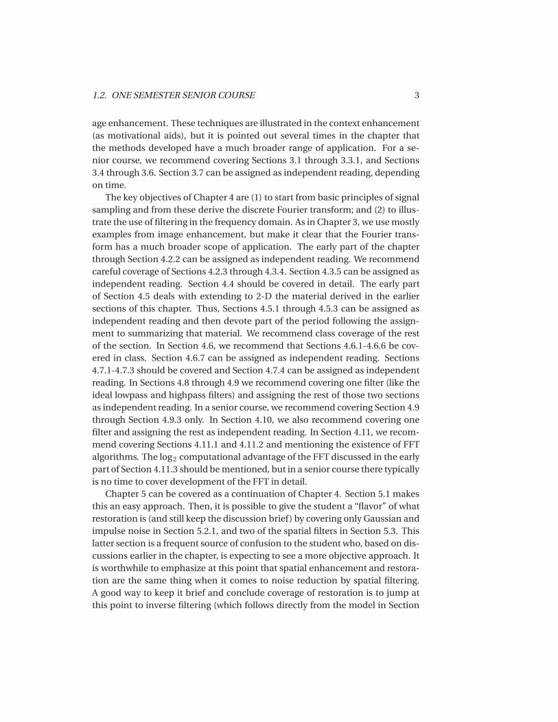
age enhancement. These techniques are illustrated in the context enhancement(as motivational aids), but it is pointed out several times in the chapter thatthe methods developed have a much broader range of application. For a se-nior course, we recommend covering Sections 3.1 through 3.3.1, and Sections3.4 through 3.6. Section 3.7 can be assigned as independent reading, dependingon time.

The key objectives of Chapter 4 are (1) to start from basic principles of signalsampling and from these derive the discrete Fourier transform; and (2) to illus-trate the use of filtering in the frequency domain. As in Chapter 3, we use mostlyexamples from image enhancement, but make it clear that the Fourier trans-form has a much broader scope of application. The early part of the chapterthrough Section 4.2.2 can be assigned as independent reading. We recommendcareful coverage of Sections 4.2.3 through 4.3.4. Section 4.3.5 can be assigned asindependent reading. Section 4.4 should be covered in detail. The early partof Section 4.5 deals with extending to 2-D the material derived in the earliersections of this chapter. Thus, Sections 4.5.1 through 4.5.3 can be assigned asindependent reading and then devote part of the period following the assign-ment to summarizing that material. We recommend class coverage of the restof the section. In Section 4.6, we recommend that Sections 4.6.1-4.6.6 be cov-ered in class. Section 4.6.7 can be assigned as independent reading. Sections4.7.1-4.7.3 should be covered and Section 4.7.4 can be assigned as independentreading. In Sections 4.8 through 4.9 we recommend covering one filter (like theideal lowpass and highpass filters) and assigning the rest of those two sectionsas independent reading. In a senior course, we recommend covering Section 4.9through Section 4.9.3 only. In Section 4.10, we also recommend covering onefilter and assigning the rest as independent reading. In Section 4.11, we recom-mend covering Sections 4.11.1 and 4.11.2 and mentioning the existence of FFTalgorithms. The log 2 computational advantage of the FFT discussed in the earlypart of Section 4.11.3 should be mentioned, but in a senior course there typicallyis no time to cover development of the FFT in detail.

Chapter 5 can be covered as a continuation of Chapter 4. Section 5.1 makesthis an easy approach. Then, it is possible to give the student a “flavor” of whatrestoration is (and still keep the discussion brief) by covering only Gaussian andimpulse noise in Section 5.2.1, and two of the spatial filters in Section 5.3. Thislatter section is a frequent source of confusion to the student who, based on dis-cussions earlier in the chapter, is expecting to see a more objective approach. Itis worthwhile to emphasize at this point that spatial enhancement and restora-tion are the same thing when it comes to noise reduction by spatial filtering.A good way to keep it brief and conclude coverage of restoration is to jump atthis point to inverse filtering (which follows directly from the model in Section

4 CHAPTER 1. INTRODUCTION

5.1) and show the problems with this approach. Then, with a brief explanationregarding the fact that much of restoration centers around the instabilities in-herent in inverse filtering, it is possible to introduce the “interactive” form of theWiener filter in Eq. (5.8-3) and discuss Examples 5.12 and 5.13. At a minimum,we recommend a brief discussion on image reconstruction by covering Sections5.11.1-5.11-2 and mentioning that the rest of Section 5.11 deals with ways togenerated projections in which blur is minimized.

Coverage of Chapter 6 also can be brief at the senior level by focusing onenough material to give the student a foundation on the physics of color (Sec-tion 6.1), two basic color models (RGB and CMY/CMYK), and then concludingwith a brief coverage of pseudocolor processing (Section 6.3). We typically con-clude a senior course by covering some of the basic aspects of image compres-sion (Chapter 8). Interest in this topic has increased significantly as a result ofthe heavy use of images and graphics over the Internet, and students usually areeasily motivated by the topic. The amount of material covered depends on thetime left in the semester.

1.3 One Semester Graduate Course (No Backgroundin DIP)

The main difference between a senior and a first-year graduate course in whichneither group has formal background in image processing is mostly in the scopeof the material covered, in the sense that we simply go faster in a graduate courseand feel much freer in assigning independent reading. In a graduate course weadd the following material to the material suggested in the previous section.

Sections 3.3.2-3.3.4 are added as is Section 3.3.8 on fuzzy image processing.We cover Chapter 4 in its entirety (with appropriate sections assigned as inde-pendent readying, depending on the level of the class). To Chapter 5 we add Sec-tions 5.6-5.8 and cover Section 5.11 in detail. In Chapter 6 we add the HSI model(Section 6.3.2) , Section 6.4, and Section 6.6. A nice introduction to wavelets(Chapter 7) can be achieved by a combination of classroom discussions and in-dependent reading. The minimum number of sections in that chapter are 7.1,7.2, 7.3, and 7.5, with appropriate (but brief) mention of the existence of fastwavelet transforms. Sections 8.1 and 8.2 through Section 8.2.8 provide a niceintroduction to image compression.

If additional time is available, a natural topic to cover next is morphologicalimage processing (Chapter 9). The material in this chapter begins a transitionfrom methods whose inputs and outputs are images to methods in which the in-puts are images, but the outputs are attributes about those images, in the sense

1.4. ONE SEMESTER GRADUATE COURSE (WITH STUDENT HAVING BACKGROUND IN DIP)5

defined in Section 1.1. We recommend coverage of Sections 9.1 through 9.4, andsome of the algorithms in Section 9.5.

1.4 One Semester Graduate Course (with Student Hav-ing Background in DIP)

Some programs have an undergraduate course in image processing as a prereq-uisite to a graduate course on the subject, in which case the course can be biasedtoward the latter chapters. In this case, a good deal of Chapters 2 and 3 is review,with the exception of Section 3.8, which deals with fuzzy image processing. De-pending on what is covered in the undergraduate course, many of the sectionsin Chapter 4 will be review as well. For Chapter 5 we recommend the same levelof coverage as outlined in the previous section.

In Chapter 6 we add full-color image processing (Sections 6.4 through 6.7).Chapters 7 and 8 are covered as outlined in the previous section. As noted inthe previous section, Chapter 9 begins a transition from methods whose inputsand outputs are images to methods in which the inputs are images, but the out-puts are attributes about those images. As a minimum, we recommend coverageof binary morphology: Sections 9.1 through 9.4, and some of the algorithms inSection 9.5. Mention should be made about possible extensions to gray-scaleimages, but coverage of this material may not be possible, depending on theschedule. In Chapter 10, we recommend Sections 10.1 through 10.4. In Chapter11 we typically cover Sections 11.1 through 11.4.

1.5 Two Semester Graduate Course (No Backgroundin DIP)

In a two-semester course it is possible to cover material in all twelve chaptersof the book. The key in organizing the syllabus is the background the studentsbring to the class. For example, in an electrical and computer engineering cur-riculum graduate students have strong background in frequency domain pro-cessing, so Chapter 4 can be covered much quicker than would be the case inwhich the students are from, say, a computer science program. The importantaspect of a full year course is exposure to the material in all chapters, even whensome topics in each chapter are not covered.

1.6 ProjectsOne of the most interesting aspects of a course in digital image processing is thepictorial nature of the subject. It has been our experience that students truly

6 CHAPTER 1. INTRODUCTION

enjoy and benefit from judicious use of computer projects to complement thematerial covered in class. Because computer projects are in addition to coursework and homework assignments, we try to keep the formal project reporting asbrief as possible. In order to facilitate grading, we try to achieve uniformity inthe way project reports are prepared. A useful report format is as follows:

Page 1: Cover page.

• Project title

• Project number

• Course number

• Student’s name

• Date due

• Date handed in

• Abstract (not to exceed 1/2 page)

Page 2: One to two pages (max) of technical discussion.

Page 3 (or 4): Discussion of results. One to two pages (max).

Results: Image results (printed typically on a laser or inkjet printer). All imagesmust contain a number and title referred to in the discussion of results.

Appendix: Program listings, focused on any original code prepared by the stu-dent. For brevity, functions and routines provided to the student are referred toby name, but the code is not included.

Layout: The entire report must be on a standard sheet size (e.g., letter size in theU.S. or A4 in Europe), stapled with three or more staples on the left margin toform a booklet, or bound using clear plastic standard binding products.1.2 OneSemester Senior Course

Project resources available in the book web site include a sample project, alist of suggested projects from which the instructor can select, book and otherimages, and MATLAB functions. Instructors who do not wish to use MATLABwill find additional software suggestions in the Support/Software section of theweb site.

1.7. THE BOOK WEB SITE 7

1.7 The Book Web SiteThe companion web site

www.prenhall.com/gonzalezwoods

(or its mirror site)

www.imageprocessingplace.com

is a valuable teaching aid, in the sense that it includes material that previouslywas covered in class. In particular, the review material on probability, matri-ces, vectors, and linear systems, was prepared using the same notation as inthe book, and is focused on areas that are directly relevant to discussions in thetext. This allows the instructor to assign the material as independent reading,and spend no more than one total lecture period reviewing those subjects. An-other major feature is the set of solutions to problems marked with a star in thebook. These solutions are quite detailed, and were prepared with the idea ofusing them as teaching support. The on-line availability of projects and digitalimages frees the instructor from having to prepare experiments, data, and hand-outs for students. The fact that most of the images in the book are available fordownloading further enhances the value of the web site as a teaching resource.

Chapter 2

Problem Solutions

Problem 2.1The diameter, x , of the retinal image corresponding to the dot is obtained fromsimilar triangles, as shown in Fig. P2.1. That is,

(d /2)0.2

=(x/2)0.017

which gives x = 0.085d . From the discussion in Section 2.1.1, and taking someliberties of interpretation, we can think of the fovea as a square sensor arrayhaving on the order of 337,000 elements, which translates into an array of size580× 580 elements. Assuming equal spacing between elements, this gives 580elements and 579 spaces on a line 1.5 mm long. The size of each element andeach space is then s = [(1.5mm)/1,159] = 1.3× 10−6 m. If the size (on the fovea)of the imaged dot is less than the size of a single resolution element, we assumethat the dot will be invisible to the eye. In other words, the eye will not detect adot if its diameter, d , is such that 0.085(d )< 1.3× 10−6 m, or d < 15.3× 10−6 m.

x/2xImage of the doton the fovea

Edge view of dot

d

d/2

0.2 m 0.017 m

Figure P2.1

9

10 CHAPTER 2. PROBLEM SOLUTIONS

Problem 2.3

The solution is

λ = c/v

= 2.998× 108(m/s)/60(1/s)

= 4.997× 106 m= 4997 Km.

Problem 2.6

One possible solution is to equip a monochrome camera with a mechanical de-vice that sequentially places a red, a green and a blue pass filter in front of thelens. The strongest camera response determines the color. If all three responsesare approximately equal, the object is white. A faster system would utilize threedifferent cameras, each equipped with an individual filter. The analysis thenwould be based on polling the response of each camera. This system would bea little more expensive, but it would be faster and more reliable. Note that bothsolutions assume that the field of view of the camera(s) is such that it is com-pletely filled by a uniform color [i.e., the camera(s) is (are) focused on a part ofthe vehicle where only its color is seen. Otherwise further analysis would be re-quired to isolate the region of uniform color, which is all that is of interest insolving this problem].

Problem 2.9

(a) The total amount of data (including the start and stop bit) in an 8-bit, 1024×1024 image, is (1024)2×[8+2] bits. The total time required to transmit this imageover a 56K baud link is (1024)2× [8+ 2]/56000= 187.25 sec or about 3.1 min.

(b) At 3000K this time goes down to about 3.5 sec.

Problem 2.11

Let p and q be as shown in Fig. P2.11. Then, (a) S1 and S2 are not 4-connectedbecause q is not in the set N4(p ); (b) S1 and S2 are 8-connected because q is inthe set N8(p ); (c) S1 and S2 are m-connected because (i) q is in ND (p ), and (ii)the set N4(p ) ∩N4(q ) is empty.

11

Figure P2.11

Problem 2.12

The solution of this problem consists of defining all possible neighborhood shapesto go from a diagonal segment to a corresponding 4-connected segments as Fig.P2.12 illustrates. The algorithm then simply looks for the appropriate match ev-ery time a diagonal segments is encountered in the boundary.

� or

� or

� or

� or

Figure P2.12

12 CHAPTER 2. PROBLEM SOLUTIONS

Figure P.2.15

Problem 2.15(a) When V = {0,1}, 4-path does not exist between p and q because it is impos-sible to get from p to q by traveling along points that are both 4-adjacent andalso have values from V . Figure P2.15(a) shows this condition; it is not possibleto get to q . The shortest 8-path is shown in Fig. P2.15(b); its length is 4. Thelength of the shortest m - path (shown dashed) is 5. Both of these shortest pathsare unique in this case.

Problem 2.16(a) A shortest 4-path between a point p with coordinates (x ,y ) and a point qwith coordinates (s , t ) is shown in Fig. P2.16, where the assumption is that allpoints along the path are from V . The length of the segments of the path are|x − s | and��y − t��, respectively. The total path length is |x − s |+ ��y − t

��, which werecognize as the definition of the D4 distance, as given in Eq. (2.5-2). (Recall thatthis distance is independent of any paths that may exist between the points.)The D4 distance obviously is equal to the length of the shortest 4-path when thelength of the path is |x − s |+ ��y − t

��. This occurs whenever we can get from pto q by following a path whose elements (1) are from V, and (2) are arranged insuch a way that we can traverse the path from p to q by making turns in at mosttwo directions (e.g., right and up).

Problem 2.18With reference to Eq. (2.6-1), let H denote the sum operator, let S1 and S2 de-note two different small subimage areas of the same size, and let S1+S2 denotethe corresponding pixel-by-pixel sum of the elements in S1 and S2, as explainedin Section 2.6.1. Note that the size of the neighborhood (i.e., number of pixels)is not changed by this pixel-by-pixel sum. The operator H computes the sumof pixel values in a given neighborhood. Then, H (aS1 + bS2) means: (1) mul-tiply the pixels in each of the subimage areas by the constants shown, (2) add

13

Figure P2.16

the pixel-by-pixel values from aS1 and bS2 (which produces a single subimagearea), and (3) compute the sum of the values of all the pixels in that single subim-age area. Let a p1 and bp2 denote two arbitrary (but corresponding) pixels fromaS1+bS2. Then we can write

H (aS1+bS2) =∑

p1∈S1 and p2∈S2

a p1+bp2

=∑

p1∈S1

a p1+∑

p2∈S2

bp2

= a∑

p1∈S1

p1+b∑

p2∈S2

p2

= a H (S1)+bH (S2)

which, according to Eq. (2.6-1), indicates that H is a linear operator.

Problem 2.20From Eq. (2.6-5), at any point (x ,y ),

g =1

K

K∑

i=1

g i =1

K

K∑

i=1

f i +1

K

K∑

i=1

ηi .

Then

E {g }= 1

K

K∑

i=1

E { f i }+ 1

K

K∑

i=1

E {ηi }.But all the f i are the same image, so E { f i } = f . Also, it is given that the noisehas zero mean, so E {ηi } = 0. Thus, it follows that E {g } = f , which proves thevalidity of Eq. (2.6-6).

14 CHAPTER 2. PROBLEM SOLUTIONS

To prove the validity of Eq. (2.6-7) consider the preceding equation again:

g =1

K

K∑

i=1

g i =1

K

K∑

i=1

f i +1

K

K∑

i=1

ηi .

It is known from random-variable theory that the variance of the sum of uncor-related random variables is the sum of the variances of those variables (Papoulis[1991]). Because it is given that the elements of f are constant and the ηi areuncorrelated, then

σ2g =σ

2f +

1

K 2 [σ2η1+σ2

η2+ · · ·+σ2

ηK].

The first term on the right side is 0 because the elements of f are constants. Thevarious σ2

ηiare simply samples of the noise, which is has variance σ2

η. Thus,σ2ηi=σ2

η and we have

σ2g =

K

K 2σ2η =

1

Kσ2η

which proves the validity of Eq. (2.6-7).

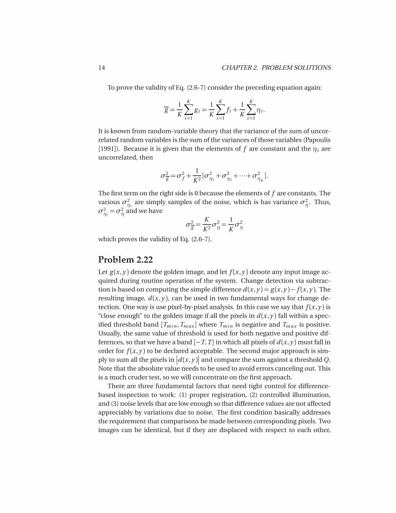
Problem 2.22Let g (x ,y ) denote the golden image, and let f (x ,y ) denote any input image ac-quired during routine operation of the system. Change detection via subtrac-tion is based on computing the simple difference d (x ,y ) = g (x ,y )− f (x ,y ). Theresulting image, d (x ,y ), can be used in two fundamental ways for change de-tection. One way is use pixel-by-pixel analysis. In this case we say that f (x ,y ) is“close enough” to the golden image if all the pixels in d (x ,y ) fall within a spec-ified threshold band [Tm i n ,Tm ax ] where Tm i n is negative and Tm ax is positive.Usually, the same value of threshold is used for both negative and positive dif-ferences, so that we have a band [−T,T ] in which all pixels of d (x ,y )must fall inorder for f (x ,y ) to be declared acceptable. The second major approach is sim-ply to sum all the pixels in

��d (x ,y )�� and compare the sum against a threshold Q.

Note that the absolute value needs to be used to avoid errors canceling out. Thisis a much cruder test, so we will concentrate on the first approach.

There are three fundamental factors that need tight control for difference-based inspection to work: (1) proper registration, (2) controlled illumination,and (3) noise levels that are low enough so that difference values are not affectedappreciably by variations due to noise. The first condition basically addressesthe requirement that comparisons be made between corresponding pixels. Twoimages can be identical, but if they are displaced with respect to each other,

15

Figure P2.23

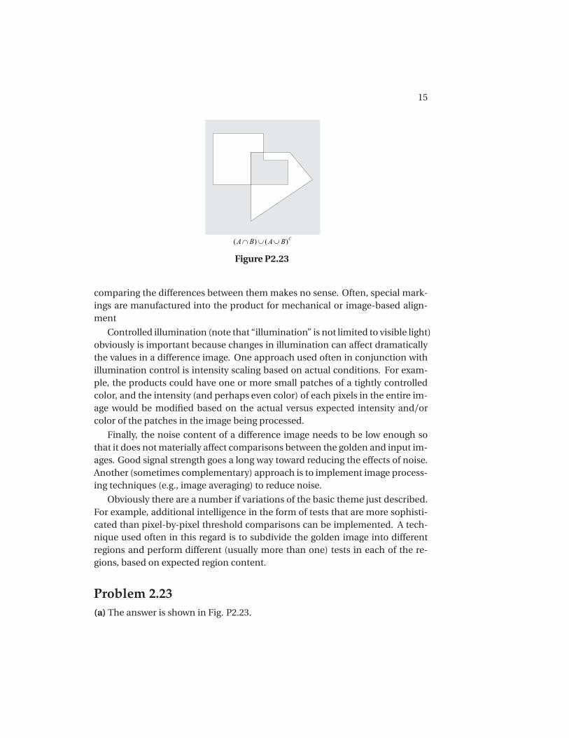
comparing the differences between them makes no sense. Often, special mark-ings are manufactured into the product for mechanical or image-based align-ment

Controlled illumination (note that “illumination” is not limited to visible light)obviously is important because changes in illumination can affect dramaticallythe values in a difference image. One approach used often in conjunction withillumination control is intensity scaling based on actual conditions. For exam-ple, the products could have one or more small patches of a tightly controlledcolor, and the intensity (and perhaps even color) of each pixels in the entire im-age would be modified based on the actual versus expected intensity and/orcolor of the patches in the image being processed.

Finally, the noise content of a difference image needs to be low enough sothat it does not materially affect comparisons between the golden and input im-ages. Good signal strength goes a long way toward reducing the effects of noise.Another (sometimes complementary) approach is to implement image process-ing techniques (e.g., image averaging) to reduce noise.

Obviously there are a number if variations of the basic theme just described.For example, additional intelligence in the form of tests that are more sophisti-cated than pixel-by-pixel threshold comparisons can be implemented. A tech-nique used often in this regard is to subdivide the golden image into differentregions and perform different (usually more than one) tests in each of the re-gions, based on expected region content.

Problem 2.23(a) The answer is shown in Fig. P2.23.

16 CHAPTER 2. PROBLEM SOLUTIONS

Problem 2.26From Eq. (2.6-27) and the definition of separable kernels,

T (u ,v ) =M−1∑

x=0

N−1∑

y=0

f (x ,y )r (x ,y ,u ,v )

=M−1∑

x=0

r1(x ,u )N−1∑

y=0

f (x ,y )r2(y ,v )

=M−1∑

x=0

T (x ,v )r1(x ,u )

where

T (x ,v ) =N−1∑

y=0

f (x ,y )r2(y ,v ).

For a fixed value of x , this equation is recognized as the 1-D transform alongone row of f (x ,y ). By letting x vary from 0 to M −1 we compute the entire arrayT (x ,v ). Then, by substituting this array into the last line of the previous equa-tion we have the 1-D transform along the columns of T (x ,v ). In other words,when a kernel is separable, we can compute the 1-D transform along the rowsof the image. Then we compute the 1-D transform along the columns of this in-termediate result to obtain the final 2-D transform, T (u ,v ). We obtain the sameresult by computing the 1-D transform along the columns of f (x ,y ) followed bythe 1-D transform along the rows of the intermediate result.

This result plays an important role in Chapter 4 when we discuss the 2-DFourier transform. From Eq. (2.6-33), the 2-D Fourier transform is given by

T (u ,v ) =M−1∑

x=0

N−1∑

y=0

f (x ,y )e−j 2π(u x/M+v y /N ).

It is easily verified that the Fourier transform kernel is separable (Problem 2.25),so we can write this equation as

T (u ,v ) =M−1∑

x=0

N−1∑

y=0

f (x ,y )e−j 2π(u x/M+v y /N )

=M−1∑

x=0

e−j 2π(u x/M )N−1∑

y=0

f (x ,y )e−j 2π(v y /N )

=M−1∑

x=0

T (x ,v )e−j 2π(u x/M )

17

where

T (x ,v ) =N−1∑

y=0

f (x ,y )e−j 2π(v y /N )

is the 1-D Fourier transform along the rows of f (x ,y ), as we let x = 0,1, . . . ,M−1.