Embed Size (px)
Citation preview

Evaluation and Rehabilitation of Damaged Beams in
Bridges
by
Salah A. Hameed
A Thesis submitted to the
Graduate School – New Brunswick
Rutgers, the State University of New Jersey
In partial fulfillment of the requirements
For the degree of
Master of Science
Graduate Program in Civil and Environmental Engineering
Written under the direction of
Professor P. N. Balaguru
And approved by
_______________________________________
_______________________________________
_______________________________________
New Brunswick, New Jersey
October, 2016

ii
Abstract of the Thesis
Evaluation and Rehabilitation of Damaged Beams in Bridges
By: SALAH AKRAM HAMEED
Thesis Director:
Dr. P.N. Balaguru
Aging infrastructures provide challenges in the areas of estimating the capacity of
partially deteriorated structural members and their Rehabilitation to restore their load
carrying capacity. Results presented in this thesis deals with assessing a deteriorated
prestressed girder of a bridge and a procedure to strengthen the weakened beam using
Fiber Reinforced Polymer (FRP) composites.
The condition of the prestressed box beam was assessed using load tests. The 46ft
span beam was part of a support system containing of 21 box girders. The test-load truck
was positioned to produce maximum possible moment on the deteriorated girder. All the
box girders were instrumented to measure maximum tensile strain at the bottom surface
of the beam. The strains at various girders were used to determine the fraction of road
carried by the deteriorated girder. Stresses and strains were computed analytically for the
test load and there is a good correlation between measured and computed values.
The second aspect of the thesis was to formulate a procedure to strengthen the
beam using FRP composites. A fraction of the pre-tensioned wire were corroded and
exposed due to environmental degradation. Carbon Fiber FRP composition repair scheme

iii
was designed assuming zero contribution from the damaged prestressing wires and
assuming complete prestress loss.
In the first scenario, amount of FRP needed to replace both prestressing force and
reinforcement capacity of the damaged wire. In the second scenario, the damaged
prestresing wires were assumed to act as non-prestressed reinforcement.
The results show that load testing provides an excellent tool for assessing
damaged beams and FRP system can be effectively used to restore the capacity of
damaged beams. Commercially available FRP systems were used for obtaining the
necessary parameters for design.

iv
ACKNOWLEDGEMENTS
I would like to take chance to express my deep gratitude to all my teachers for their
guidance and consultation and to my colleagues and friends for their friendship. Special
thanks are addressed to the following for their invaluable assistance in the completion of
this work:
To my advisor, Professor P.N. Balaguru, for his wisdom and guidance throughout
my education at Rutgers University.
To Professor Husam Najm, for his support during the program and my research.
To CAIT (Center for Advanced Infrastructure and Transportation) for the
Research Assistant appointments during my studies.
To my colleague, Alaa Abd Ali, for his help and support during different phases
of the research, study, and for his friendship.
Finally, I would like to express my gratitude to my wife Hiba Al-Adhami, for her
support and help during all phases of my study.

v
Table of Contents Abstract of the Thesis ...................................................................................................................... ii
ACKNOWLEDGEMENTS ................................................................................................................... iv
List of Tables .................................................................................................................................. vii
List of Figures ................................................................................................................................ viii
Chapter One ..................................................................................................................................... 1
Introduction ..................................................................................................................................... 1
1.1 Objective of the study ............................................................................................................ 3
Chapter Two ..................................................................................................................................... 4
State of the art ................................................................................................................................. 4
Chapter Three ................................................................................................................................ 11
Research Program .......................................................................................................................... 11
Chapter Four .................................................................................................................................. 13
Field Testing ................................................................................................................................... 13
4.1 Description of the Test Bridge ............................................................................................. 13
4.2.1 Gage Location: .................................................................................................................. 16
4.2.3 Sensors: ............................................................................................................................. 18
4.2.4 Data acquisition system and setup ................................................................................... 20
A. CR6 Data logger ................................................................................................................. 22
B. CDM-VW305 Dynamic Vibrating Wire Measurements...................................................... 23
C. 12V Battery and CH200 regulator: ..................................................................................... 24
D. Laptop with LoggerNet software Program: ....................................................................... 25
4.3 Test set up: ........................................................................................................................... 26
4.4 Field Test: ............................................................................................................................. 29
Installation and Field setup .................................................................................................... 29
Test Vehicle: ............................................................................................................................... 31
4.5 Result of live load test .......................................................................................................... 32
Chapter Five ................................................................................................................................... 37

vi
Analytical Competitions ................................................................................................................. 37
5.1 Load (sharing) distribution among beams and beam properties .................................... 37
5.2. A. Maximum Absolut Moment............................................................................................ 41
5.2. B. Another Approach to find M: .......................................................................................... 43
5.3.1 Influence of Asphalt layer on Distribution of load among the girder ........................... 45
In this part, the influence of the thickness of the asphalt layer on the concrete deck has been
included: .................................................................................................................................... 45
5.3.2 Prestress force from the bottom strand ....................................................................... 46
5.3.3 Fixed end moment ........................................................................................................ 47
Chapter Six ..................................................................................................................................... 49
Study for alternative solution for the bridge ................................................................................. 49
6.1 Introduction: ........................................................................................................................ 49
Chapter Seven ................................................................................................................................ 85
Design of Repair System for Damaged Prestressed Girders Using Fiber Reinforced Polymer (FRP)
....................................................................................................................................................... 85
7.1 Background .......................................................................................................................... 85
7.2 Summary of Proposed Repair .............................................................................................. 87
7.3 Initial repair using epoxy mortar and surface preparation .................................................. 88
7.4 FRP Repair design ................................................................................................................. 88
7.5. A. Repair design calculation ............................................................................................... 90
Non-linear analysis: ........................................................................................................................ 92
7.5. B. Repair design calculation ................................................................................................ 94
Chapter Eight ................................................................................................................................. 95
CONCLUSIONS ................................................................................................................................ 95
REFERENCES ................................................................................................................................... 97

vii
List of Tables
Table 3.1 - Pre-stressed properties…………………………………………………… 13
Table 3.2 - Location and Number of Sensors………………………………………… 16
Table 3.3a - Data for strain and displacement – Span 1……………………………… 31
Table 3.3b - Data for strain and displacement – Span 2……………………………… 33
Table 6.1 - AASHTO girder section properties ……………………………………… 51

viii
List of Figures
Figure 4.1 - Bridge side view ………………………………………….………. 14
Figure 4.2 - Structure No. 1223-153, Route 35 ………………………………... 14
Figure 4.3 - Bridge’s top view ……………………………………...………….. 15
Figure 4.4 - Locations of Sensors ………………………………..…………….. 17
Figure 4.5 - Vibrating wire strain gauge (4000) ……………..………………… 19
Figure 4.6 - 8510 Potentiometer ……………………………………………..… 20
Figure 4.7 - Data Acquisition Diagram ……………………………………..…. 21
Figure 4.8 - Data Acquisition System during Monitoring ………………………21
Figure 4.9 - Campbell Science CR6 Data …………………………………...…. 22
Figure 4.10 - CDM-VW305 Dynamic Vibrating …………………………….… 23
Figure 4.11 - 12V Battery and CH200 …………………………………..…….. 24
Figure 4.12 - LoggerNet computer program …………………………..………. 25
Figure 4.13 - Strain gage and PT Flexure Testing …………………..………… 27
Figure 4.14 - Strain gauge and PT8510 Transducer / Flexure Testing ……...… 28
Sample Testing Concrete Blocks
Figure 4.15 - Installed 4000 Vibrating wire strain Gauges ……………………..29

ix
Figure 4.16 - Installed 4000 Vibrating wire strain Gauges and PT 8510 ………30
Figure 4.17 - The weights and distances for the load vehicle ……………...….. 31
Figure 4.18 - Strain gauges scrawling for Beams 3, 4, 5, and 6 …………...….. 36
Figure 5.1 - Strains along the cross section of the bridge .………………………... 38
Figure 5.2 - Bottom bars ………………..……………………………………… 39
Figure 5.3 - Top bars …………………………………………………….……... 39
Figure 5.4 - cross section in box-girder ………………………………………... 39
Figure 5.5 - The relation between the distribution factor and strain………......... 41
Figure 5.6 - vehicle test location on the bridge ……………………………........ 41
Figure 5.7 - SFD and BMD for the beam ………………………………….…… 44
Figure 5.8 - cross section in box-girder with bottom reinforcement ………........ 44
Figure 5.9 - The relation between the Asphalt’s Modulus of elasticity……...….. 46
and strain
Figure 5.10 - The relationship between the fixed end moment …………….…… 48
and the strain
Figure 6.1 - Cross section in bridge deck …………………………………..….…50
Figure 6.2 - Girder spacing versus span length …………………………...……... 52
Figure 6.3 - Type 4 girder ……………………………………………...………… 53

x
Figure 6.4 - Girder details ……………………………………………………… 57
Figure 7.1 - Damaged Beams BM3 and BM 4 in Span 1 ……………………… 86
Figure 7.2 - Damaged Beams BM18 and BM19 in Span 1 ……………………. 86
Figure 7.3 - Damaged Beams BM3 and BM4 in Span 4 ………………………. 87
Figure 7.4 - Damaged Beams BM18 and BM19 in Span 4 ……………………. 87
Figure 7.5 - Typical detail of FRP Repair. Beam width is 36-inches………….. 89
FRP width shall be 30-inches
Figure 7.6 - calculate the maximum moment capacity using …………………. 93
non-linear approach

1
Chapter One
Introduction
Continuously operating instrumented structural health monitoring (SHM) systems
are becoming a practical alternative to supersede visual inspection for assessment of
condition and health of civil infrastructure, such as bridges. Although, the large amount
of data from an SHM system needs to be converted to useable information, it is still
considered a great challenge to which special signal processing techniques must be
applied. This study is devoted to the identification of abrupt, anomalous, and potentially
onerous events in the time histories of static, instantaneous sampled strains recorded by a
multi-sensor SHM system installed in a major bridge structure and operating
continuously for three types of tests ( static, dynamic, and crawling). Such events may
result from, among other causes, sudden settlement of foundation, ground movement,
excessive traffic load or failure of posttensioning cables.
It is much more efficient to provide in-place repair girders than to completely shut
down or reroute interstate highway traffic to rebuild a bridge. An effective in-place repair
is needed for these bridge girders. The pre-repair load test and a post-repair load test are
required to determine the effectiveness of the FRP repair. The pre-repair load test results
provide a baseline for which the post-repair load test results can be compared. The pre-
repair load test will also provide information to better understand the current bridge
behavior. Thus, it is important to have updated information on structural condition and
performance of bridges in order to earlier detect any worrying signs of decline and
undertake protective countermeasures.

2
In this study, the pre-repair static load test was described for a bridge in Perth
Amboy, New Jersey. In the test, bridge girders were instrumented, and data was collected
while a NJDOT load truck was positioned in predetermined locations along the bridge
surface. The results of the tests were recorded, and the measured bridge response was
examined to gain insight into the structural behavior of the system. Conclusions about the
behavior of the bridge were reported, and ideas were introduced about the possible
variation of bridge behavior with strain and displacement. A portion of the load test was
focused on using the principle of superposition to determine whether the existing bridge
superstructure behaves as a linear-elastic system under service-level loads.
One of the major challenges of a SHM study is making sense of large amounts of
data that continuously operating SHM systems produce. For the success of SHM, the data
needs to be reduced into manageable volumes and forms, and then that information needs
to be extracted and then be developed as knowledge about structural condition. There are
likely to be major differences between the relatively basic expectations and requirements
of infrastructure managers and the ambitions of systems designers; the latter usually
originally academic.
Transportation infrastructure authorities have long recognized the need to keep
their bridges healthy and to this end have implemented various inspection and
management programs. The current health monitoring practice is primarily based on
visual inspection. Due to high manpower demand, such inspections cannot be performed
frequently. Other drawbacks of visual inspection based condition assessment include
inaccessibility of critical parts of the structure and lack of information on actual loading.
These shortcomings lead to subjective and inaccurate evaluations of bridges’ safety and

3
reliability. As a result, some bridges may be retrofitted or replaced, while in fact they are
sound. On the other hand, existing damages in other bridges may not be identified until
they become expensive to repair or dangerous for structural integrity.
1.1 Objective of the study
The objective of the research described in this thesis is to perform the pre-repair
static load test required to determine the effectiveness of the FRP repair and analyze the
results. The pre-repair test will provide a baseline to which the post-repair test can be
compared. The test data is also analyzed to determine both the behavior of the cracked
girders and the effectiveness of superposition.

4
Chapter Two
State of the art
Beginning in the late 1950’s in the United States, the continuous prestressed
bridges have been developments to making multi-span and connecting the ends of the
girders over the supports. This began an investigation for improvement, which included
the connection between the girders by diaphragm connecting. Timely in this process, the
Portland Cement Association noticed that continuity could be beneficial in three different
ways (Kaar, et al 1960). First, both the deflection and maximum moments at the mid span
of girder could reduce by the continuity over support, also, approximately 5 to 15 percent
fewer strands could be allowed to be used when using the continuous girders, and also
more than this percent could be achieved (Freyermuth 1969). Second, the long term
durability of a girder could be developed by eliminating the joints over the support since
that will reduce the amount of water and salt, which are the main factors causing the
deterioration in the concrete. Also, the riding surface could be improved by eliminating
the joints. Third, the reserve load capacity in the event of an overload condition could be
provided by the continuity of a girder.
On the other hand, over the past fifty years, many states have been familiar with
the benefits of making precast, prestressed multi-girder bridges continuous by connecting
the girders with a continuity diaphragm. Further, there has not been as much agreement
on either the methods used for design of these system or details used for the continuity
connection, although there is agreement on the benefits of continuous construction.

5
Surveys show that 21% of the bridges in the US bridge inventory are prestressed, as are
more than half of the new bridges being built each year (TRB 2000).
Prestressed concrete bridges are often made of simple-span girders. The
performance of these bridges can be improved by providing a positive moment
connection between the girders after they are set in place. This makes the bridge simple
span for structural dead loads, but continuous for all superimposed loads. In addition to a
more favorable distribution of loads, these bridges have a number of practical and
economic benefits, such as improved durability, elimination of bridge deck joints, and
reduced maintenance costs.
The New Jersey Department of transportation (NJDOT) is currently involved in a
bridge rehabilitation and replacement program where each of the state’s bridges is
assessed to determine its rehabilitation needs. One of the bridges identified for
rehabilitation is located in Perth Amboy NJ.
Most precast, prestressed girders used for bridge construction are non-composite
for self-weight and the dead load of the deck but are later made composite by the addition
of a cast-in place concrete deck. Therefore, both composite and non-composite properties
must be considered in the design process. Also, unique to this type of construction, the
construction sequencing can have a large influence on the behavior of the system.
Once a multi-span system is made continuous, thermal restraint moments will
develop and induce additional stresses in the system. Some design methods do not
consider these influences; however, the stresses caused by the thermal restraint moments
may be significant and have been considered in this study.

6
Considering just some of these influences, it can be seen that the behavior of a
system made of precast, prestressed concrete made continuous can be difficult to predict.
As some responses begin to influence the behavior of other material properties, the
validity of using the law of superposition begins to be questioned, making the prediction
of the behavior of these systems even more difficult.
Various studies have been conducted since but, except for minor modifications,
the fundamental analysis methods have remained the same. Recent developments in
analysis methods and material behavioral research, coupled with long-term experimental
and field observations, have raised questions as to the validity of accepted analysis
methodology for these bridges. Recent research has determined that the long-term
behavior of ‘continuous for live load’ bridges is not predicted accurately by industry-
accepted methods of analysis. Specifically, these analytical models predict an alteration
in the distribution of moment in the structure, caused by shrinkage of concrete, which is
not confirmed by experimental data. The greatest challenge in modeling ‘continuous for
live load’ is determining a technique for simulating the complex creep and shrinkage
behavior of prestressed concrete and the shrinkage and cracking behavior of reinforced
concrete. A logical first step would be to model a simple span structure and be sure that
the creep, shrinkage and cracking behaviors can be accurately modeled. When this is
confirmed, these modeling techniques will be available for use in modeling ‘continuous
for live load’ bridges. This study attempts to simulate creep due to prestress and dead
load in the girders, differential shrinkage between the deck and girder and cracking in the
deck of a single span bridge.

7
Finally, this type of construction had the following advantages over conventional
simple span bridges: i) the maintenance costs associated with bridge deck joints and deck
drainage onto the substructure, were reduced or eliminated. ii) Continuity improved the
appearance and riding quality of the bridge. iii) Seismic performance was improved
(Miller et al 2004). iv).The structural economy of a continuous design and the elimination
of deck joints, guaranteed an initial economic advantage (Freyermuth 1969).
Health monitoring of civil infrastructures has achieved considerable importance in
recent years, since the failure of these structures can cause immense loss of life and
property. However, the large size and complex nature of the civil–structural systems
render the conventional visual inspection very tedious, expensive, and sometimes
unreliable, thus necessitating investigations for the development of automated techniques
for this purpose. Many monitoring techniques have been reported in the literature, the
most popular among the researchers in civil engineering being those based on the
response of low-frequency vibration on the structures. Using these techniques, the first
few mode shapes are extracted and processed to assess the locations and the amount of
damage. Some of the prominent algorithms employing this principle include the change
in stiffness method (Zimmerman and Kaouk 1994), the change in flexibility method
(Pandey and Biswas 1994), and the damage index method (Kim, Jeong-Tae 2003).
Basically, SHM should be broadly defined as “the use of insitu, nondestructive sensing
and analysis of structural characteristics, including the structural response, for the
purpose of identifying if damage has occurred (Level 1 of diagnostics), determining the
location of damage (Level 2), estimating the severity of damage (Level 3), and evaluating

8
the consequences of damage on structural serviceability, reliability and durability (Level
4)” (C. Sikorsky 1999).
The development of structural health monitoring technology for surveillance,
evaluation and assessment of existing or newly built bridges has now attained some
degree of maturity. On-structure long-term monitoring systems have been implemented
on bridges in Europe, the United States, Canada, Japan, Korea, China, and other
countries. Bridge structural health monitoring systems are generally envisaged to:
(i) validate design assumptions and parameters with the potential benefit of improving
design specifications and guidelines for future similar structures; (ii) detect anomalies in
loading and response, and possible damage/deterioration at an early stage to ensure
structural and operational safety; (iii) provide real-time information for safety assessment
immediately after disasters and extreme events; (iv) provide evidence and instruction for
planning and prioritizing bridge inspection, rehabilitation, maintenance and repair;
(v) monitor repairs and reconstruction with the view of evaluating the effectiveness of
maintenance, retrofit and repair works; and (vi) obtain massive amounts of in situ data for
leading-edge research in bridge engineering, such as wind- and earthquake-resistant
designs, new structural types and smart material applications (Ko, J. M., and Y. Q. Ni
2005).
To date, numerous structure health monitoring methodologies and systems have
been proposed, and some of them have been applied on the full-scale bridge structures:
e.g., the Alamosa Canyon Bridge (Farrar, C. R., and S. W. Doebling 1997), the I-10
Bridge (Todd et al. 1999), the Hakucho Bridge in Japan (Abe et al. 2000), the Bill
Emerson Memorial Bridge in Missouri (Çelebi et al. 2004), and the Tsing Ma Bridge in

9
Hong Kong (Wong 2004), to name a few. Though these examples demonstrated the
significant potential of SHM, the cost of obtaining the relevant information for structure
health monitoring on large structures is high (Rice and Spencer 2009). For example, the
Bill Emerson Memorial Bridge is instrumented with 84 accelerometer channels with an
average cost per channel of over $15 K, including installation (Jang, Shinae, et al. 2010).
Continuously operating structure health monitoring systems generally produce
various “raw” signals, such as displacements, accelerations, strains, stresses,
temperatures, wind velocities, or signals resulting from some form of analytical
processing of the raw data, e.g. natural frequencies or power spectra. Because of the
character of signals recorded by structure health monitoring systems, i.e. time series
sampled over long periods of time and at regular intervals, such data naturally lend
themselves to examination using the extensive and proven tools offered by the time series
analysis and statistical process control. The concepts of the time series analysis have
successfully been applied to numerous problems, notably in the field of econometrics,
where they have been used, for example, to investigate stock prices, production and
prices of various commodities, and interests rates (Wei, 1993). Little has been reported,
with the exception of the aforementioned study by Sohn et al. (2000), about application
of time series analysis in the area of SHM of civil infrastructure. Another publication is
that of Moyo and Brownjohn (2002b) who used intervention analysis for assessing the
impact of various events during construction of a bridge on the recorded time series of
strains. The present study uses several existing procedures of the time series analysis to
understand and extract information from the strain data recorded on a bridge structure.

10
The main objective is to identify abrupt events sustained by the bridge and possible
structural change or damage.

11
Chapter Three
Research Program
The concept of structural health monitoring has been the subject of research over
the last few years, especially in civil and structural engineering where the major concern
for the infrastructure is the old age. These studies have direct to initiatives towards the
development and employment of new sensing technologies. According to the tough
environments found in the construction industry, and the large size of civil engineering
structures, such sensors should be strong, tough, easy to use and economical.
The result reported in this dissertation deals with:
Lab testing for the equipment that used in the field test, this equipment should
prepare and calibrate before using in the field test. Also, this equipment have
attached to the concrete beam in the lab and test for the flexural test to ensure the
correct reading for the sensors and data acquisition.
Field testing of Prestress concrete girder, the test was in the site to collect the data
from the girders of the bridge, and this test have done with install 21 sensors for
the strain and eight sensors for displacement, and connect these sensors to data
acquisition, and connect the data acquisition to the computer to collect the data.
Analysis an actual bridge to verify the measurements and interpretation of load-
test result, and analysis the data that have gotten from the bridge to compare with
the standard

12
Analysis for replacing the box-girder by I-section girder to avoid the damage
which was happened for the girder by prevented the water from drainage. Also,
the cost for I- section girder less than the box-girder.
Analysis of damage girder and strengthened Prestress concrete girder, and
recommendation for repairing the Prestress concrete girder.
Procedure for repairing damaged girder by using FRP to avoid the bridge
replacement and prevent them girder from the corrosion by the time.
A typical SHM system comprises an array of sensors, sensor warning hardware, a
host computer and communication hardware and software. Sensors play the important
role of providing information about the state of strain, stress and temperature of the
structure. Their selection for a particular application is governed by application, sensor
sensitivity, power requirements, robustness and reliability. Most SHM systems reported
in the literature have focused on traditional sensing technologies such as electrical
resistance train sensors, vibrating wire strain gauges and piezoelectric accelerometers.
While the traditional sensors are robust and strong enough for civil engineering
applications they often require many cables to support them, and for long distance
monitoring these cables suffer from electromagnetic interference (EMI).

13
Chapter Four
Field Testing
4.1 Description of the Test Bridge
The bridge (structure No. 1223-153) is located on NJ Route 35 over Perth Amboy
Connector (NJ 440), Abandoned Perth Amboy (South Plainfield Branch) and Conrail.
The bridge has four spans (3-main & 1-approach), is simply supported, is composite, is a
pre-stressed concrete box beams in main span, and has voided slab beams in the south
approach span. This bridge was built in 1960 and underwent rehabilitation in 1972. The
rehabilitation repaired the spalls in pre-stressed beams with exposed strands in Spans 1
and 4. Cracks in the pavement on the approach roadway and over the abutment deck
joints have been partially sealed. The bridge is in serious condition due to the
superstructure. The bridge consists of 21 adjacent 3’-0” wide x 2’-3” high x 236’ long
pre-stressed concrete beams and an average 5.5” thick composite concrete deck. On each
side of exterior concrete girder, curbs and guardrails are located. The annual average
daily traffic was 22,300 vehicles and truck ADT is 4% in 2004 for this bridge. For
testing, a 58,000 lb 3-axle truck was driven over the bridge. All 21 concrete beams were
pre-stressed to have the properties in Table 4.1:
Table 4.1 Pre-stressed properties
strength of, f’c 5000 psi
Strength of, f’ci 4000 psi
Pre-stressing steel yield 248,000 psi
Reinforcing steel yield 40,000 psi
pre-stressing steel 7/16 Ø uncoated
Stressed- relived seven wires strans. Fi 27,000 psi, per strand
14
Figure 4.1 Bridge side view
Figure 4.2 - Structure No. 1223-153, Route 35

15
The instruments used in this investigation have been provided by several well-known
companies. The datalogger and its belongings were provided by Campbell Science, while
the dynamic strain sensors were provided by Geokon. Finally the displacement
potentiometers were provided by Celesco. The following will be introduced to describe
details of the instruments:
1- Gage Location
2- Instrumentations
3- Sensors
4- Data acquisition system and setup
Figure 4.3 - Bridge’s top view

16
4.2.1 Gage Location:
The strain gage has been attached in the middle of the span because of the
expected maximum strains in this location. There were 17 strain gages and 8 PTs
installed in the bottom of the beams in the post-tension rods. In addition, 17 strain gages
were attached to the bridge, one per beam. Two beams from each side did not have strain
gages because of its walkway. Four PTs were also attached to four beams on each side.
Generally, these settings were chosen to discuss:
Effects of the post-tensioning rod, especially for beam 3 and beam; these beams
were damaged
Load transfer from beam 3 and beam 4 to other beams
The bending of the first four beams from each side, four beams chosen to
compare between the first two that damaged and beams 5 and 6 respectively, to
see what is the difference in displacement
Strain Gage PT
Beam 3 to Beam 19 17
Beam 1 to beam 4 4
Beam 16 to beam 19 4
Table 4.2 Location and Number of Sensors

17
Figure 4.4 Locations of Sensors

18
4.2.2 Instrumentations:
The instruments that were used for this investigation were Geokon 4000A
vibrating wire strain gages and Celesco 8510 displacement potentiometers. Both strain
gages and PTs were attached underneath the beams of the bridge. To connect these
instruments to a computer and collect data, these instruments needed a data acquisition
device. The gages connected to a 16 x 18 inches enclosure; this enclosure contained a
CR6 data logger, a CDM-VW305, a 12V battery, and a charger. The 4000A strain gages
connected to a CDM-VW305, and the CDM-VW305 connected to a CR6. The 8510 PTs
connected directly to a CR6 data logger. The CR6 data logger connected to the laptop.
The CR6 data logger received power from the battery while the charger charged the
battery. All other instruments in the board received power from the CR6. The lead wires
connected the 8510 PTs and the strain gages to the enclosure. All connection was
completed on the day of the field test. However, access under the bridge was not allowed
during the day of the field test, but. NJDOT prepared all the appropriate papers to allow
us access at a future time.
4.2.3 Sensors:
All strain gages’ data was recorded to the CDM-VW305 then from the CDM-
VW305 to the CR6 data logger. Then the PTs’ data was recorded directly to the CR6
data logger. These strain gages and PTs attached directly to the bottom of the beams
for the bridge by using the instant adhesive glue. The installation of the gages was
done by three research assistants from Rutgers the State University of New Jersey.
Two types of instruments were used in this investigation:
19
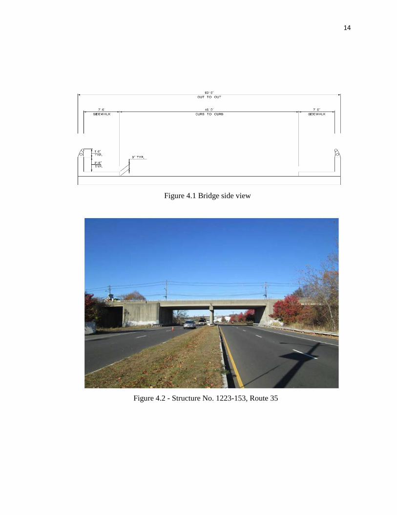
1- The Geokon model 4000 vibrating wire strain gage, is intended primarily
for long-term or short-term strain measurement on any steel or concrete
structure such as tunnel lining, arches, struts, piles, bridges, sheet pilings,
etc. The strain gage uses the vibrating wire principle: a length of steel wire
is tensioned between two mounting blocks that are attached to a concrete
beam. Deformations of the surface causes the two mounting blocks to move
relative to one another, thus altering the tension in the steel wire. The
tension in the wire is measured by plucking the wire and measuring its
resonant frequency of vibrating. The wire is plucked, and its resonant
frequency measured, by means of an electromagnetic coil positioned next to
the wire. See Figure 4.5 (Manual from Geokon Inc. 2014)
2- The Celesco PT 8510 displacement potentiometer, detects and measures
linear position and velocity using a flexible cable made from stainless steel
and a spring-loaded spool with an optical encoder sensor. The cable
measurement for the model that was used in this investigation was ranging
Figure 4.5 Vibrating wire strain gauge (4000)

20
between (0 – 6 inches). This model is designed for rough environments,
injecting modeling, and detecting the linear displacement for structures from
the gravity load. The accuracy of this model is 0.04 % from the full stroke.
The total weight of the sensor is 3 lb.
To ensure the compatibility between the PT 8150 and the CR6 there
is a special setup that should be provided for the PT 8150. The input voltage
for the PT 8150 should range between (0 – 5 volte), the operating
temperature should range between (0 – 160 F), and the maximum vibration
is 10g. (See figure 4.6)
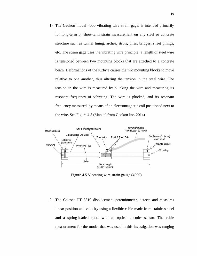
4.2.4 Data acquisition system and setup
During this investigation, the CR6 data logger was used for the control system
and measurement, the CDM-VW305 connected the strain gages to the CR6 data logger,
and the battery and charger gave power to the system. In addition, the CR1000 data
logger, CR3000 data logger, CS-CPI data logger and AM16/32 relay multiplexers were
Figure 4.6 - 8510 Potentiometer
21
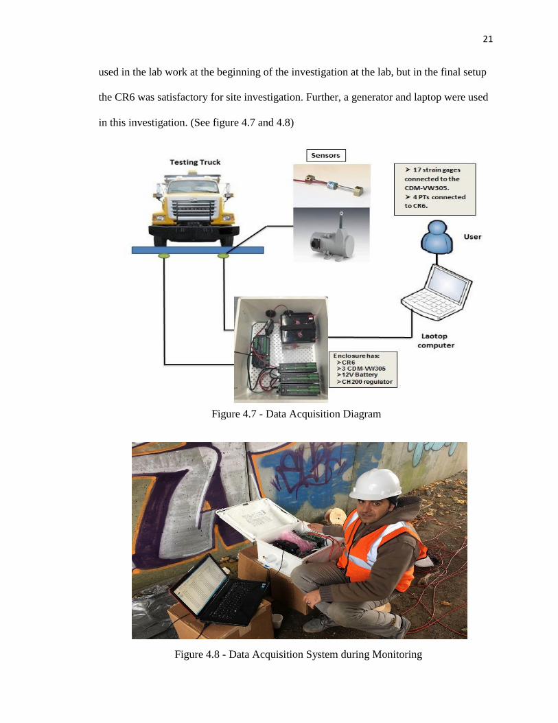
used in the lab work at the beginning of the investigation at the lab, but in the final setup
the CR6 was satisfactory for site investigation. Further, a generator and laptop were used
in this investigation. (See figure 4.7 and 4.8)
Figure 4.7 - Data Acquisition Diagram
Figure 4.8 - Data Acquisition System during Monitoring

22
A. CR6 Data logger
The CR6 data measurement and control system manufactured by Campbell
scientific, Inc. is a powerful core component of a data-acquisition system, adding
faster communications. Further, it combines the best features of all data loggers,
has low power requirements (flexible power input from solar panel, DC power
supply, 12V battery, or USB), has built in USB, and is a compact size. CR6-series
data loggers feature universal (U) terminals, which allow connection to virtually
any sensor-analog, digital, or smart, onboard communication via Ethernet 10/100.
It has a micro SD card drive for extended memory requirements, support for serial
sensors with RS-232 and RS-485 native, and CPI for hosting Campbell high-
speed sensors and distributed modules (CDMs). It is programmable with CRBasic
or SCWin program generator, completely PakBus compatible, and has a shared
operating system (OS) with the popular CRBasic CR1000 and CR3000 data
loggers. (Campbell Scientific, Inc.2015). (See figure 4.9)
Figure 4.9 - Campbell Science CR6 Data

23
B. CDM-VW305 Dynamic Vibrating Wire Measurements
The CDM-VW305 is an 8-channel link between sensors and data loggers that
takes lees time to gather data, and gathers the data simultaneously. This link uses an
excitation mechanism that ensures the vibrating wire sensor operates in a continuously
vibrating state. The interface measures the resonant frequency of the wire between
excitations using the patented vibrating wire spectral-analysis technology. The CDM-
VW305 provides very fine measurement resolution and also limits the effects of external
noise by distinguishing between signals and noise based on frequency content. Because
of this technology, signals can be carried through longer cables, providing compatibility
between the sensors and the CR6 data logger. . (See figure 4.10).
The CDM-VW305 interfaces with standard vibrating wire sensors, giving much
faster and more accurate. The CDM-VW305 has eight channels per module;
synchronized across multiple modules. Furthermore, it has dynamic measurement rates of
20 to 333 Hz. In addition, the CDM-VW305 has low power requirements; it can work by
a flexible power input from solar panel, DC power supply, or 12V battery.
Figure 4.10 - CDM-VW305 Dynamic Vibrating

24
C. 12V Battery and CH200 regulator:
The 12V battery supplied the power for all instruments in the enclosure and it was
charging from the CH200 regulator. The 12V battery includes a 24in. attached cable that
terminates in a connector for attaching the battery to a CH200 regulator. The CH200
regulator was connected directly to power source. The CH200 allows charging from
various sources: solar panels, AC wall chargers, and a generator. The CH200 allows
simultaneous connection of two charging sources such as solar panel and AC wall
charger. The CH200 has the ability to monitor both load and battery current. (See figure
4.11).
Figure 4.11 - 12V Battery and CH200

25
D. Laptop with LoggerNet software Program:
The CR6 data acquisition system is operated by a computer-coded program.
Campbell Scientific team was helping to create a program code that is compatible with 17
strain gages, eight PTs, the CR6, and the CDM-VW305. To collect and control necessary
data at the live load test, first the LoggerNet computer application had to be installed and
then the conformed program code on the data acquisition laptop computers was
processed. The LoggerNet software supports the CR6 program generation, real-time
display of data-logger measurements, graphing, and retrieval of data files. (See figure
4.12)
Figure 4.12 - LoggerNet computer program

26
4.3 Test set up:
To ensure the accuracy and performance of the field instrumentation, a lab test was
performed at the Civil Engineering Laboratory at Rutgers University. In addition, it was
necessary to check the field procedure, and then compare those results with the results
from the lab test.
One concrete beam sample was prepared and tested in the lab. The beam made of
plain concrete according to C192, and the cross sectional dimension of the concrete beam
were 6 x 6 inches and the total length was 20 inches, while the clear span was 18 inches.
Compressive strength of cylindrical concrete specimens had been tested according to
C39. The average compressive strength of the cylinders was 6250 psi. According to
ACI318, the modulus of rupture was given by:
𝑓𝑟=7.5 𝑓′𝑐
In this lab test, it was found that flexural strength was 593 psi.
The test setup was designed for 50% of the flexural strength. For that, the maximum
flexural strength in the lab test had not exceeded 300 psi to avoid the brittle failure of
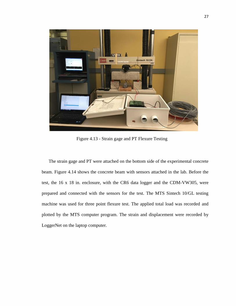
plain concrete. See Figure (4.13).
27
The strain gage and PT were attached on the bottom side of the experimental concrete
beam. Figure 4.14 shows the concrete beam with sensors attached in the lab. Before the
test, the 16 x 18 in. enclosure, with the CR6 data logger and the CDM-VW305, were
prepared and connected with the sensors for the test. The MTS Sintech 10/GL testing
machine was used for three point flexure test. The applied total load was recorded and
plotted by the MTS computer program. The strain and displacement were recorded by
LoggerNet on the laptop computer.
Figure 4.13 - Strain gage and PT Flexure Testing

28
The moment of inertia of the cross section of the concrete beam was 108 in4, and the
designed flexural strength was 300 psi, therefore, the expected applied moment was
10,800 lb.in. The MTS machine was setup to stop when the applied moment reached
10,800 lb.in, and this moment was expected to develop when the machine load reached
2400 lb.
The load was applied continuously with a deflection control until the load reached
2400 lb. with a loading rate equal to 0.05 in/min.
Figure 4.14 - Strain gauge and PT8510 Transducer / Flexure
Testing Sample Testing Concrete Blocks

29
As a result, the reported data showed an adequate compatibility between the field
instrumentation and the MTS machine with an off error less than 2%.
4.4 Field Test:
Installation and Field setup
In advance, the sensors were attached to the bridge by the research team on the first
week of December, 2015. The boom lift truck was used to reach the bottom of the bridge
to attach the sensors. The lead wire was used to connect the sensors to the enclosure, all
17 strain gages were connected to the CDM-VW305 and 8 PTs were connected to the
CR6 data logger correctly. The connection was checked by each sensor’s specific
resistance value using the multi-meter. The State of New Jersey Department of
Transportation (NJDOT) and the Center for Advance of Infrastructure and Transportation
(CAIT) provided access to the site. The traffic arrangement and the loading test vehicle
supplied were by the Maintenance of Traffic (MOT). (See figure 4.15 and 4.16)
Figure 4.15 - Installed 4000 Vibrating wire strain Gauges

30
After the sensors were installed, the 2-axle pre-loaded dump truck was used, the
truck path decided by the sensors location. Three types of tests (parking test, crawling
test, and dynamic test) were performed through four spans of the bridge, and each type of
test has been performed three times to confirm data reproducibility and to establish the
reliable characteristics of the beams’ behavior. The parking test was done by setting the
truck in the middle of the span for five minutes, the crawling test was done by driving the
truck 5 miles/hour over the span, and the dynamic test was done by drive the truck 30
miles/ hour through the path. When the truck was crossing over the structure, the sensors
recorded the data simultaneously to the CR6 data logger, and the data was collected to the
laptop by using the LoggerNet software program. The data logger collected data for the
strain gages and the PTs every 0.2 seconds (200 milliseconds), its mean recorded five
times per second.
Figure 4.16 - Installed 4000 Vibrating wire strain Gauges and PT 8510

31
Test Vehicle:
The weights and dimensions of the test vehicle were recorded before the
investigation. The live load was the weight of the vehicle in the station; the vehicle’s total
weight was 57,800 lbs. It is a three-axle truck, with a front-wheel weight of 9 kips for
each wheel, a rear-wheel weight of 10 kips for each wheel, and a middle-wheel weight of
10 kips for each wheel. The distance between the front and middle wheels is 16’9” and
the distance between the middle and a rear wheel is 4’9”. Figure 4.17 shows the distances
and the weights. The truck driver was instructed to drive along the path designated by
paint marks for each trip.
Figure 4.17 - The weights and distances for the load vehicle

32
4.5 Result of live load test
The data logger program began to collect data from CR6. As the CR6 data logger
collected data from sensors, the test vehicle started its journey. The data was recorded
onto a laptop computer in raw form. The raw data collected from strain gauges was
converted to strain data using a pre-coded program, while the raw data collected from the
PTs was converted from electrical signals to displacement values by using a preceded
program before being plotted on graphs. The test was carried out for two spans, with each
span having 21 beams, while each test had three iterations to ensure data quality. Tables
4.3a and 4.3b below show the maximum strain and maximum displacement for each
beam in the middle of the span.
Table 4.3a Data for strain and displacement – Span 1
Beam No. StrainX10-6 Disp.(in) StrainX10-6 Disp.(in)
1
2
3 16 0.0035 16 0.0035
4 - 0.0065 - 0.0065
5 28 0.008 28 0.008
6 28 0.0065 27 0.0065
7 25 25
8 18 19
9 14 15
10 10.5 10.5
11 8.5 8
12 10 11
13 13 15
14 19 21
15 24 25
16 23 0.003 23 0.003
17 27 0.008 28 0.008
18 16 0.005 16 0.005
19 17.5 0.003 18 0.003
20
21
StrainX10-6 Disp.(in)
8
10
13
0.003516
19
23
-
27
27
25
20
15
11
0.0065
0.008
0.0065
0.003
0.008
0.005
0.003
22
26.5
15.5
17
Park Test 1 Park Test 2 Park Test 3

33
Beam No. StrainX10-6 Disp. StrainX10-6 Disp. StrainX10-6 Disp.
1
2
3 16 0.006 17 0.006 18 0.006
4 6.5 0.004 7 0.004 6.5 0.004
5 22 0.004 23 0.004 22 0.004
6 22 0.006 23 0.006 23 0.006
7 18 18 18
8 16 14 14
9 15 12 14
10 12 10 12
11 12 8 13
12 13 10 14
13 16 12 14
14 17 14 14
15 20 20 20
16 24 0.0065 25 0.0065 25 0.0065
17 24 0.0045 25 0.0045 25 0.0045
18 7 0.004 7.5 0.004 7 0.004
19 17 0.0065 18 0.0065 19 0.0065
20
21
Crawing Test 1 Crawing Test 2 Crawing Test 3
Beam No. StrainX10-6 Disp.(in) StrainX10-6 Disp.(in) StrainX10-6 Disp.(in)
1
2
3 14 0.0055 15 0.0055 16 0.0055
4 - 0.005 - 0.005 - 0.005
5 23 0.005 26 0.005 25 0.005
6 25 0.008 27 0.008 23 0.008
7 22 25 20
8 17 18 15
9 12 15 10
10 8 9 7
11 6 7 7
12 8 10 8
13 11 13 15
14 17 18 17
15 23 24 24
16 25 0.003 25 0.003 25 0.003
17 26 0.0075 26 0.0075 27 0.0075
18 18 0.006 17.5 0.006 18.5 0.006
19 19 0.003 18 0.003 21 0.003
20
21
Dynamic Test 1 Dynamic Test 2 Dynamic Test 3

34
Beam No. StrainX10-6 Disp. StrainX10-6 Disp.
1
2
3 16 0.005 15 0.005
4 6.5 0.004 5 0.004
5 21 0.004 22 0.004
6 23 0.0045 23 0.0045
7 19 20
8 14 15
9 14 13
10 10 9
11 8 8
12 8 10
13 10 13
14 12 15
15 16 17
16 21 0.006 25 0.006
17 20 0.004 25 0.004
18 5 0.004 6 0.004
19 15 0.005 19 0.005
20
21
StrainX10-6 Disp.
21 0.004
22 0.0045
17
15 0.005
6 0.004
7
8
12
13
11
8
6 0.004
18 0.005
16
18
20 0.006
Park Test 1 Park Test 2 Park Test 3
25 0.004
Beam No. StrainX10-6 Disp. StrainX10-6 Disp. StrainX10-6 Disp.
1
2
3 16 0.006 17 0.006 18 0.006
4 6.5 0.004 7 0.004 6.5 0.004
5 22 0.004 23 0.004 22 0.004
6 22 0.006 23 0.006 23 0.006
7 18 18 18
8 16 14 14
9 15 12 14
10 12 10 12
11 12 8 13
12 13 10 14
13 16 12 14
14 17 14 14
15 20 20 20
16 24 0.0065 25 0.0065 25 0.0065
17 24 0.0045 25 0.0045 25 0.0045
18 7 0.004 7.5 0.004 7 0.004
19 17 0.0065 18 0.0065 19 0.0065
20
21
Crawing Test 1 Crawing Test 2 Crawing Test 3
Table 4.3b Data for strain and displacement – Span 2

35
Beams 3, 4, 5, and 6 were chosen to plot and show the differences in strain
between the damaged beams (3 and 4) and the intact beams (5 and 6). Figure (4.15)
describes the data that was recorded in the field test. The first max strain (Max 1) location
was the point at which the front wheels of the test vehicle crossed the sensor location for
the first beam (Beam 6), Also the same value maximum strain for the second beam
(Beam 5) was recorded. In the same manner, the second max strain (Max 2) location was
the point at which the rear wheels of test vehicle crossed the sensor location for Beams 5
and 6. The third maximum strain (Max 3) location was where the rear wheels of the test
vehicle crossed the sensor location for Beam 3. The fourth max strain (Max 4) location
was where the rear wheel of the test vehicle crossed the sensor location for Beam 4. All
strains are shown in Figure (4.18).
Beam No. StrainX10-6 Disp. StrainX10-6 Disp. StrainX10-6 Disp.
1
2
3 20 0.004 15 0.004 18 0.004
4 6 0.0045 5 0.0045 5.5 0.0045
5 25 0.006 20 0.006 25 0.006
6 25 0.0045 20 0.0045 25 0.0045
7 21 15 21
8 16 12 16
9 14 12 12
10 11 11 10
11 9 9 9
12 7 7 8
13 10 10 10
14 13 13 13
15 x x x
16 21 0.009 22 0.009 21 0.009
17 22 0.011 23 0.011 22 0.011
18 x 0.008 x 0.008 x 0.008
19 x 0.009 x 0.009 x 0.009
20
21
Dynamic Test 1 Dynamic Test 2 Dynamic Test 3

36
As indicated in Figure 4.18, there is a difference between the intact beams (5 and
6) and the damaged beams (3 and 4). The max strain of both intact beams shows a similar
trend of higher strain under the heavier (rear-wheel) load than under the front wheels.
Moreover, the strain for the intact beams is higher than the strains shown for the damaged
beams.

37
Chapter Five
Analytical Computations
This chapter provides details of analytical procedure to estimate the strains
measured during the load test testing. This study was conducted to find the influence of
many variables on the value of the strain. There are many variables have significant
effect to change the value of the correct strain. The various steps are:
Distribution load sharing among the beams and beam properties.
Computation maximum Absolut moment among the beam.
Properties of cross section.
Computation of maximum strain.
Variables that affect maximum strain.
Use of these variables for accurate prediction of maximum strain.
These variables are calculated to compare with the strain that has gotten from the
load-test in the site. Beam number 7 from the Table 3.3a was used for the parametric
study. The maximum strain for this beam was 25 micro.
5.1 Load (sharing) distribution among beams and beam properties
The wheel load is distributing unequally between the adjacent girders. In this part,
the maximum load distribution factor has been calculated by the area under the strain-
distance curve in Figure 5.1 as follow:

38
Total area under curve = 173
Maximum strain = 25
Distribution factor % =
* 100% = 14.5%
Check Ig:
Ig = 112 [ 36 * 273
– 26.75 * 163 ] = 49,918.3 in
4
y =
= 0.94 in
ɣ=
= 1.17”
n = 𝐸𝑠𝐸𝑐 =
√ = 7.2
Distance Strain
1.5 19
4.5 22
7.5 25
10.5 24
13.5 21
16.5 18
19.5 14
22.5 11
25.5 8
28.5 5
31.5 2
33.5 0
Figure 5.1 - Strains along the cross section of the bridge

39
A ctr = As * n
(
) (Ʃ 𝐴=544+𝑛−1𝐴𝑠+𝑛−2𝐴𝑠′)
ȳ = 14”
Itr. = 𝑛𝐴𝑠 (27−2.94−ȳ)2 +𝑛′𝐴𝑠′ (ȳ−ɣ)
2 + (36 27
3/12) +36 27 (27/2− ȳ)
2 − 26.75
163/12 − 26.75 16 (27/2− ȳ)
2
Itr = 53,051 in4
Figure 5.3 - Top bars Figure 5.2 - Bottom bars
Figure 5.4 - cross section in box-girder

40
ft =
= 1.53 K/in
2 = 1530 lb/in
2
Ec = 57000 5000 = 4030.5 Ksi
Є =
= 0.38 * 10
-3 = 380 micro strain
Reduced strain after applying the distribution factor was:
0.145 * 380= 55.1
The obtained strain from analysis 55.1μm was higher than the reported strain from
the field test 25 μm. There were many reasons for that. First, the end restriction of the
span may case reduction in the strain. In the analysis, the bridge assumed simply
supported without any restriction at the ends, however, in the real case there were some
restrictions due to the continuity of the bridge deck. Furthermore, the expected modulus
of elasticity was higher than the calculated one because the section was prestressed, so
the concrete may compressed and increased the modulus of elasticity. Moreover, the real
inertia of the section was higher than the calculated inertia because of the extra mild steel,
also prestressed strands. Finally, the effect of compression stress due to prestressed stand
in the tension zone had not considered in the analysis, and this might be the major reason
for difference.

41
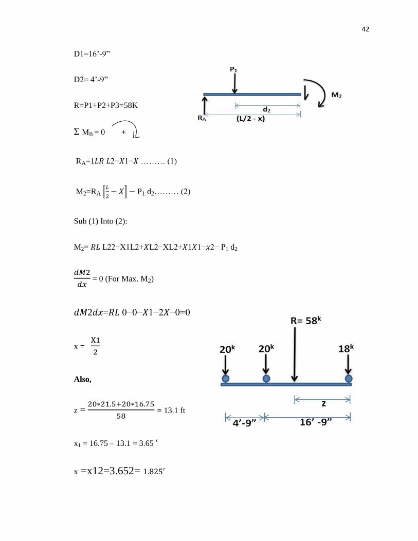
5.2. A. Maximum Absolut Moment
The theoretical maximum absolute moment have been calculated using the same
wheel load from the truck was used in the field test. The wheel load shown in the Figure
5.2.
Input:
P1= 20K
P2= 20K
P3= 18K
L= 46ft
Figure 5.6 - vehicle test location on the bridge
15
17
19
21
23
25
27
29
31
0.1 0.11 0.12 0.13 0.14 0.15 0.16
Str
ain
(μ
)
Distribution factor
Series1
Figure 5.5 - The relation between the distribution factor and strain
42
D1=16’-9”
D2= 4’-9”
R=P1+P2+P3=58K
Ʃ MB = 0 +
RA=1𝐿𝑅 𝐿2−𝑋1−𝑋 ……… (1)
M2=RA [
𝑋] P1 d2……… (2)
Sub (1) Into (2):
M2= 𝑅𝐿 L22−X1L2+𝑋L2−XL2+𝑋1𝑋1−𝑥2− P1 d2
= 0 (For Max. M2)
𝑑𝑀2𝑑𝑥=𝑅𝐿 0−0−𝑋1−2𝑋−0=0
x =
Also,
z =
= 13.1 ft
x1 = 16.75 – 13.1 = 3.65
x =x12=3.652=

43
L = 46 ft , R = 58k
RA =
[
– (3.65 – 1.825) ]
RA = 26.7k
(maximum expected reaction on the left pier)
ML = 26.7 * 21.175 – 20 * 4.75
ML = 470.4 K.ft
This moment represents the maximum moment if the beam resists the entire load. Since
the load is shared by other beams, the moment resisted by the damaged beam is estimated
using the procedure presents in the next section.
ML = 0.145 * 470.4 = 68.2 K.ft
5.2. B. Another Approach to find M:
In this approach, the maximum moment has been calculated assuming the load is
symmetric and the maximum moment in the middle of the span.
M = 20 * 20.635 = 412.7 K.ft
F’c = 5000 psi
Ig = 49,918 in4, A = 544 in
2 A(strand Ø 7/16) = 0.115 in
2

44
Figure 5.7 - SFD and BMD for the beam
Figure 5.8 - cross section in box-girder with bottom reinforcement

45
5.3.1 Influence of Asphalt layer on Distribution of load among the girder
In this part, the influence of the thickness of the asphalt layer on the concrete deck
has been included:
Ig = 49,918 in4
n = n’ = 𝐸𝑠/𝐸𝑐 =
√ = 7.2
Actr = As * n asph.
n1 = Easph./𝐸𝑐 =
√ = 0.25
𝑛 𝐴𝑠 ( (
)) (
) ( )
𝐴 𝑛 𝐴𝑠 𝑛 𝐴𝑠 𝑛 𝐴 𝑠
ȳ = 18.5 “
Itr=𝑛 𝐴𝑠 (33−2.94−ȳ)2+𝑛′𝐴𝑠′ (ȳ−(1.17+6))
2+36 27
3/12+36 27 (12.5-27/2)
2 − 26.75
163/12−26.75 16 (16/2-7)
2+6 9
3/12+6 9 (18.5−6/2)
2
Itr = 67,728 in4
ft =
* (33-18.5) = 0.6 k/in
2
Є =
= 0.15 * 10
-3 = 150 micro strain
Also,
E ( Asphalt )
psi
Strain (Micro
strain )
0.5 * 106 160
0.75 * 106 155
1 * 106 150
1.25 * 106 144
1.5 * 106 138

46
5.3.2 Prestress force from the bottom strand
To include the effect of prestress force on the strain of the girder from the bottom strand,
eight strand were assumed deteriorated.
Then,
The total workable strands in the girder = 26 – 8 = 18 strands
P = 18 * 0.115 * 120 = 248.4 K
e = 33 – 18.5 – 0.94 = 13.56 in
Me = 248.4 * 13.56 / 12 = 281 K/in2
fbottom =
* ( Me –ML)
=
– K/in
2
Є =
= 0.11 * 10
-3 = 110 micro strain
270
275
280
285
290
295
300
305
310
315
320
325
0 0.5 1 1.5 2
Sta
rin
(μ
)
EAsphalt * 106 psi
Strain
Figure 5.9 - The relation between the Asphalt’s Modulus of elasticity and strain

47
5.3.3 Fixed end moment
In the ideal case the maximum moment was calculated assuming there wasn’t any
restriction at the ends. In the real case there was a significant effect for this restriction. To
include the effect of end restrain for possible zero moment were discussed, and the results
shown in Figure 5.10.
1- 0.975L = 44.85 ft
RA =
= 13.32 K
M = 13.32 * 20.6 – 10 * 4.75 = 227 k.ft
ft =
= 0.74 k/in
2
Є =
= 0.183 * 10
-3 = 183 micro strain
2- 0.95L = 43.7 ft
RA =
= 13.29 K
M = 13.29 * 20.025 – 10 * 4.75 = 218.6 k.ft
ft =
= 0.71 k/in
2
Є =
= 0.176 * 10
-3 = 176 micro strain
3- 0.925L = 42.55 ft
RA =
= 13.26 K
M = 13.26 * 19.45 – 10 * 4.75 = 210.4 k.ft
ft =
= 0.68 k/in
2
Є =
= 0.169 * 10
-3 = 169 micro strain
4- 0.9L = 41.4 ft
RA =
= 13.22 K

48
M = 13.22 * 18.875 – 10 * 4.75 = 202 k.ft
ft =
= 0.65 k/in
2
Є =
= 0.162 * 10
-3 = 162 micro strain
320
325
330
335
340
345
350
355
360
365
370
0.88 0.9 0.92 0.94 0.96 0.98
Stra
in (μ
)
Fixed end Moment * L (ft.)
Series1
Figure 5.10 - The relationship between the fixed end moment and the strain

49
Chapter Six
Study for alternative solution for the bridge
6.1 Introduction:
In the box- girder adjacent bridge that we have investigated in this study, the
water ingress to the joint between girders and cased a sever deterioration to the box-
girders of the bridge. The type of the geometry and the shear key that connected the box-
girders of the bridge to each other may the main reason for this deterioration by holding
the water in place.
In the original geometry, the bridge was consisting of four spans with total span
length equal to 236 ft. the second and the fourth pier were deteriorated severely. For that,
an alternative geometry for the spans has been proposed. The proposed new span
geometry has two equal spans with 120 ft. each and one pier in the middle.
Moreover, an alternative geometry for the girders has been suggested in this study
in case of any future plan to replace the bridge. Type IV precast prestrssed concrete beam
suggested instated of the box-girder. All the detailed calculations for analysis the new
bridge have been elaborated and reported in this chapter.

50
Given:-
1. span data:
Overall beam length= 121 ft
Design beam length= 120 ft
2- Cross section data:
Number of lanes=2
Number of beams= 7
Beam spacing=6 ft
3- Dead loads:
Figure 6.1 - Cross section in bridge deck

51
Slab thickness = 7 in
Barrier weight= 0.2 k/ft
Future wearing surface= 0.02 k/ft2
Wearing width=25 ft
Wc=145 lb/ft3
4- Live loads:
HL-93 Design truck +Design lane load
5- Deck properties:
Deck concrete 28- day strength =4 ksi
f'c=4 ksi
ksifwE cc 40745)145.0(*3300033000 5.1'5.1
6- Beam properties:
Beam concrete 28- day strength =7 ksi
ksifwE cc 48217)145.0(*3300033000 5.1'5.1
Beam concrete strength at release = 6 ksi
ksifwE cc 44636)145.0(*3300033000 5.1'5.1
52
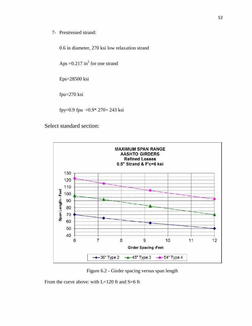
7- Prestressed strand:
0.6 in diameter, 270 ksi low relaxation strand
Aps =0.217 in2 for one strand
Eps=28500 ksi
fpu=270 ksi
fpy=0.9 fpu =0.9* 270= 243 ksi
Select standard section:
From the curve above: with L=120 ft and S=6 ft
Figure 6.2 - Girder spacing versus span length

53
The best section is (Type 4) with 54 in depth
The properties of sections as elaborated in Table 5.1:
Table 5.1 AASHTO girder section properties
Figure 6.3 - Type 4 girder

54
Effective flange width – AASHTO (4.6.2.6.1)
A- Interior beam:
For the interior beam, the effective flange width may be taken as the least of:
1- One quarter of the effective span length : 120 feet for simple spans
(0.25) (120) (12) = 360 in
2- Twelve time the average thickness of the slab, 7 in , plus the greater of
The web thickness: 8 in
One-half of the top flange of the girder: 42 in
(0.5) (20) =10 in
The greater of these two values is 10 in and:
(12) (7) + (10) = 94 in
3- The average spacing of adjacent beams: 6 ft
(6) (12) = 72 in
The least of these is 72 in and therefore, the effective flange width is (72 in).
B- For the exterior beam, the effective flange width may be taken as one- half the
effective flange width of the adjacent beam, 72 in, plus the least of:

55
1- One-eighth of the effective span length: 120 feet
(0.125) (120) (12) = 180 in
2- Six times the average thickness of the slab: 7 in, plus the greater of:
One-half of the web thickness: 8 in
(0.5) (8) = 4 in
One- quarter of the top flange of the girder: 20 in
(0.25) (20) = 5 in
The greater of these two values is 5 in and:
(6) (7)+5 = 47 in
3- The width of the overhang: 2.5 ft
(2.5) (12) = 30 in
The least of these is 30 in and the effective flange width is:
(0.5) (72) + 30 = 66 in
Composite section properties:
845.04821
4074
beam
deck
E
En
The transformed deck area is:
A= (72) (.845) (7) = 425.88 in2

56
Io =(72) (0.845 (7)3/12 = 1739 in
4
A Yb Ayb D Ad2 Io Io+Ad
2
Deck 425.9 57.5 24489.25 21.26 192501.52 1739 194240
Beam 788.4 24.75 19512.9 11.49 104084.64 260403 364487
Total 1214.4 44002.15 558727
Property Interior beam Exterior beam
Icomp(in4) 558727
ybc(in) 36.24
ytc(in) 17.76
yslab top(in) 24.76
Sbc(in3) 15417.4
Stc(in3) 31460
Sslab top(in3) 22565.7

57
Dead loads:
Interior beam
The dead loads, DC, acting on the non-composite section are:
Figure 6.4 - Girder details

58
Weight of beam = 0.821 k/ft
Slab weight= (72/12) (7/12) (0.15) = 0.525 k/ft
The dead load, DC, acting on the composite section is:
Barrier
(0.2) (2)/7 = 0.057 k/ft
The dead load, DC, acting on the composite section is:
Future wearing surface allowance (FWS):
(0.02) (25)/7 = 0.0714 k/ft
Distribution of live load:
Interior beam
eg=yt+ts = 29.249 + 7/2 = 32.75 in
183.14074
4821
deck
beam
E
En
The longitudinal stiffness parameter is :
422 1308462)75.32*44.788260403(183.1)( inAeInK gg

59
Distribution of live load for moment AASHTO (4.6.2.2.2b)
Check the range of applicability
koftSS .65.3
kointt ss .7125.4
koftLL .12024020
koftSS .65.3
koinkk gg .1308462700000010000 4
koNN bb .74
For one lane loaded:
1.0
3
3.04.0
121406.0
s
g
Lt
K
L
SSg
38.0)7)(120(12
1308462
120
6
14
606.0
1.0
3
3.04.0
g
For the fatigue limit state, remove the multiple presence factor.
316.02.1
38.0g
For two or more design lane loaded:

60
1.0
3
2.06.0
125.9075.0
s
g
Lt
K
L
SSg
534.0)7)(120(12
1308462
120
6
5.9
6075.0
1.0
3
2.06.0
g
Distribution of live load for shear:
Check the range of applicability
koftSS .65.3
kointt ss .7125.4
koftLL .12024020
koftSS .65.3
koinkk gg .1308462700000010000 4
koNN bb .74
For one design lane loaded:
6.025
636.0
2536.0
Sg

61
For the fatigue limit state, remove the multiple presence factor.
5.02.1
6.0g
For two or more design lane loaded:
67.035
6
25
62.0
35122.0
22
SSg
Limit states:
The most common limit states for prestressed concrete beam design are:
Strength I
1.25DC+1.5DW+1.75(LL+IM)
Strength II
1.25DC+1.5DW+1.35(LL+IM)
Service I
1.0DC+1.0DW+1.0(LL+IM)
Service III
1.0DC+1.0DW+0.8(LL+IM)
Fatigue
0.75(LL+IM)

62
Beam stresses:
In order to determine the number of required strands, first calculate the maximum
tensile stress in the beam for Service III limit state. The number of required strands is
usually controlled by the maximum tensile stresses in the beam meet the tensile stress
limit. For simple span beams, the maximum tensile force is at mid span at the extreme
bottom beam fiber. The tension service stress at the bottom beam fibers can be calculated
using:
bc
LLFWSbarrier
b
slabbeambottom
S
MMM
S
MMf
8.0
(Service III limit state)
The non-composite moments are:
ftkM beam .14788
120*821.0 2
ftkM slab .9458
120*525.0 2
The composite moments are:
ftkM barrier .6.1028
120*057.0 2
ftkM FWS .5.1288
120*0714.0 2

63
Live load plus dynamic load allowance :( HL-93)
)33.1( trucklaneILL MMDFM
ftkM lane .11528
120*64.0 2
ftkM truck .1883
1952k.ft1883)*1.330.534(1152ILL
M
Interior beam- stresses due to dead load and live load.
)(16.412*)4.15417
1952*8.05.1286.102
10521
9451478( tksifbottom

64
Preliminary strand arrangement:
The development of a strand pattern is a cyclic process. Two design parameter
need to be initially estimated: the total prestress losses and the eccentricity of the strand
pattern at mid span.
The total required prestress force can be calculated using:
bmc
bottomtene
S
e
A
ffP
1
The concrete stress limit for tension, all loads applied, and subjected to severe corrosion
condition table (5.9.4.2.2-1), is
ksiff cten 25.070948.00948.0 '
)(35 estimatedksif pT
ksif pj 5.202)270)(75.0(
ksif pe 5.167355.202
kAfP pspee 34.36217.0*5.167* (For one strand)
e = -20 inches (estimated)
kPe 7.1233
10521
)20(
4.788
1
)16.4(25.0

65
The number of strand required is:
94.3334.36
7.1233
Try use 34 strands.
The distance from the bottom of the beam to the center of gravity of the prestressing
strands is:
iny 75.434
8*46*104*102*10
The eccentricity of the prestressing strands at the midspan is:
e = 24.75- 4.75= 20 in
At the ends of the beam the distance from the bottom of the beam to the center of gravity
of the prestressing strands with 10 strand harped at the 0.4 span point, is:
iny 94.1634
)4446485052(26*84*82*8
The eccentricity of the prestressing strands at ends of the beam is:
e=24.75- 16.94= 7.81 in

66
Prestress loss- Low relaxation strand
We will assume that the prestressing strands are jacked to an initial stress of o.75fpu
Girder creep coefficients for final time due to loading at transfer
H=70%
V/S= 4.5
ti= 1 day
tf=20000 days
t=20000-1=19999 days
865.0)5.4(13.045.1)/(13.045.1 SVKvs
7142.061
5
1
5'
c
ff
K 9981.019999)6(461
19999
461 '
tf
tK
ci
td
118.09.1),(
itdfhcvsif tKKKKtt
1715.1)1)(9981.0)(7142.0)(1)(865.0(9.1),(118.0
if tt
Girder creep coefficient at time of deck placement due to loading introduced at transfer
td=180 days
t=180-1= 179 days
170*008.056.1008.056.1 HKhc

67
828.0178)6(461
178
461 '
tf
tK
ci
td
118.09.1),(
itdfhcvsid tKKKKtt
972.0)1)(828.0)(7142.0)(1)(865.0(9.1),(118.0
id tt
Girder creep coefficient at final time due to loading at deck placement
t=20000-180 = 19820 days
9981.019820)6(461
19820
461 '
tf
tK
ci
td
118.09.1),(
itdfhcvsdf tKKKKtt
6348.0)180)(9981.0)(7142.0)(1)(865.0(9.1),(118.0
df tt
Deck creep coefficients:
Deck creep coefficients at final time due to loading at deck placement
V/S= 5
t=20000-180 = 19820 days
koSVKvs .0.08.0)5(13.045.1)/(13.045.1
141
5
1
5'
c
ff
K

68
9977.019820)4(461
19820
461 '
tf
tK
ci
td
118.09.1),(
itdfhcvsdf tKKKKtt
8217.0)180)(9977.0)(1)(1)(8.0(9.1),(118.0
df tt
Transformed section coefficients for time period between transfer and deck placement:
epg = 20 in
),(7.01(11
12
ifb
g
pgg
g
ps
ci
p
id
ttI
eA
A
A
E
EK
855.0
)1715.1*7.01(260403
20*4.7881
4.788
202.5
4463
285001
12
idK
Transformed section coefficients for time period between deck placement and final time:
epc=36.24 – 4.75 = 31.49 in
),(7.01(11
12
ifb
c
pcc
c
ps
ci
p
df
ttI
eA
A
A
E
EK
8642.0
)1715.1*7.01(558727
49.31*4.12141
4.1214
202.5
4463
285001
12
dfK

69
Elastic shortening: AASHTO (5.9.5.2.3a)
For the first iteration, calculate fcgp using a stress in the prestressing steel equal to 0.9 of
the stress just before transfer.
Pt=(0.9)(202.5)(5.202) = 948 k
inkM beam .1773612*8
120*821.0 2
I
yM
I
yeP
A
Pf beamtt
cgp )(
ksifcgp 29.1260403
)20(*17736
260403
)20))(20(*948(
4.788
948
cgp
ci
p
pES fE
Ef
ksif pES 23.829.1*4463
28500
ksif pt 27.19423.85.202
For the second iteration, calculate fcgp using a stress in the prestressing steel of 194.27
ksi
Pt=(194.27)(5.202) = 1010.6 k
ksifcgp 472.1260403
)20(*17736
260403
)20))(20(*6.1010(
4.788
6.1010

70
ksif pES 4.9472.1*4463
28500
ksif pt 1.1934.95.202
Pt=(193.1)(5.202) = 1004.5 k
ksifcgp 455.1260403
)20(*17736
260403
)20))(20(*5.1004(
4.788
5.1004
ksif pES 291.9455.1*4463
28500
ksif pt 2.193291.95.202
Pt=(193.2)(5.202) = 1005.02 k
ksifcgp 456.1260403
)20(*17736
260403
)20))(20(*02.1005(
4.788
02.1005
ksif pES 3.9456.1*4463
28500
ksif pt 2.1933.95.202
Pt=(193.2)(5.202) = 1005.02 k
ksifcgp 456.1260403
)20(*17736
260403
)20))(20(*02.1005(
4.788
02.1005
ksif pES 3.9456.1*4463
28500

71
Losses: time of transfer to time of deck placement
Shrinkage of girder concrete, (5.9.5.4.2a)
310*48.0* tdfhsvsbid KKKK
ininbid /00039.010*48.0*1*9977.0*02.1*8.0 3
ksiKEf idpbidpSR 6.98642.0*28500*00039.0
Creep of girder concrete AASHTO (5.9.5.4.2b)
ididbcgp
ci
p
pCR KttfE
Ef ),(
ksif pCR 81.78642.0*972.0*456.14463
28500
The relaxation loss pRIf may be assumed equal to 1.2 ksi for low-relaxation strands.
Losses: time of deck placement to final time.
02.170*014.02014.02 HKhs

72
Shrinkage of girder concrete AASHTO (5.9.5.4.3a)
310*48.0* tdfhsvsbif KKKK
ininbid /00039.010*48.0*9981.0*9977.0*02.1*8.0 3
000039.000039.0 bidbifbdf
0 dfpbdfpSD KEf
Creep of girder concrete AASHTO (5.9.5.4.3b)
comp
compFWSbarrierslabcd
I
yMM
I
yMf
)(
ksifcd 03.1558727
)49.31(*12)5.1286.102(
260403
)20(*12*945
0),(),(),( dfdfbcd
c
p
dfidbifbcgp
ci
p
pCD KttfE
EKttttf
E
Ef
8642.0*8217.0*03.14821
28500
8642.0)972.01715.1(456.14463
28500
pCDf
ksif pCD 92.5

73
Shrinkage of deck concrete AASHTO (5.9.5.4.3c)
Strain due to shrinkage
310*48.0* tdfhsvsddf KKKK
ininddf /000421.010*48.0*9981.0*9977.0*02.1*865.0 3
c
dpc
dfd
cddddf
cdfI
ee
Att
EAf
1
)),(7.01(
558727
)26.21(499.31
4.1214
1
)8217.0*7.01(
)4074)(504(000421.0cdff
ksifcdf 205.0
)),(7.01( dfbdfcdf
c
p
pSS ttKfE
Ef
ksif pSS 65.1)8217.0*7.01(8642.0)205.0(4821
28500
Total losses:
dfpSSpRpCDpSDidpRpCRpSRpLT fffffff )()( 21
ksif pLT 08.24)65.12.192.50()2.181.76.9(
ksifff pESpLTpT 37.333.908.24

74
Strand arrangement:
Now that the total loss in the prestressing steel stress has been calculated, check if
the preliminary strand pattern and eccentricity are still valid. The calculated effective
stress in the prestressing steel is:
For interior beam
(169.12)(0.217) = 36.7 k
The number of strands required
The preliminary strand arrangement with 34 strands is still good.
ksif pe 12.16938.335.202
kPe 7.1233
10521
)20(
4.788
1
)16.4(25.0
6.337.36
7.1233

75
Service limit state:
Calculate the beam stress limits for two conditions: temporary before losses for
the release condition and after all losses for the service condition. For the temporary
before losses condition (5.9.4.1):
Tension:
ksiuseksiksifc 2.02.0232.060948.00948.0 '
Compression:
ksifc 6.36*6.06.0 '
At all service limit state after all losses (5.9.4.2)
Tension: severe corrosion condition:
ksifc 25.070948.00948.0 '
Compression:
Due to effective prestress and permanent loads:
ksifc 15.37*45.045.0 '
Due to live load and one-half the sum of effective prestress and permanent loads:
ksifc 8.27*4.04.0 '

76
Due to effective prestress, permanent loads, and transient loads:
'6.0 cw f
The reduction factor w is equal to (1) if the flange slenderness ratio is not greater than
15. The slenderness ratio is the ratio of the flange width to depth:
28.107
72
depthflange
widthflane
Since this value is not greater than 15, w is equal to (1) and the stress limit is:
ksifcw 2.47*1*6.06.0 '
The stress limits for the concrete deck slab at the service limit state:
Compression:
Due to effective prestress and permanent loads:
ksifc 8.14*45.045.0 '
Due to effective prestress and permanent loads, and transient loads:
ksifcw 4.24*1*6.06.0 '
The total area of prestressing steel, the initial or transfer prestressing force, and the
effective prestressing force are:
2378.734*217.0 inAps

77
kAfP psptt 4.1425)378.7)(2.193())((
kAfP pspee 84.1247)378.7)(13.169())((
Stresses at transfer:
I
yM
I
yeP
A
Pf beamtt
bottom )(
(Service I limit state)
(Service I limit state)
At the harp point due to the initial prestress force and the beam dead load
inkMbeam .7.1726012*4.1438
)(8.2260403
)751.24(17260
260403
)751.24)(20)(1425(
44.788
1425cksifbottom
)(54.0260403
)249.29(17260
260403
)249.29)(20)(1425(
44.788
1425cksiftop
At the ends of transfer length due to the initial prestress force and the beam dead load:
The transfer length is 60 strand diameter or 36 inches. Therefore, the end of the transfer
length is 36 inches from the end of the beam or 30 inches from the centerline of bearing,
the 0.0208 point. The eccentricity of the prestressing force is:
e=8.3 in
I
yM
I
yeP
A
Pf beamtt
top )(

78
inkMbeam .144012*120
)(79.2260403
)751.24(1440
260403
)751.24)(3.8)(1425(
44.788
1425cksifbottom
)(82.0260403
)751.24(1440
260403
)751.24)(3.8)(1425(
44.788
1425cksiftop
Stresses at service condition:
The service stresses, assuming tension at the bottom fibers, can be calculated using:
c
LLFWSbarrierslabbeameebottom
I
yMMM
I
yMM
I
yeP
A
Pf
)8.0()()(
(Service III limit state)
c
LLFWSbarrierslabbeameetop
I
yMMM
I
yMM
I
yeP
A
Pf
)()()(
(Service I limit state)
Interior beam:
At end of transfer length due to the effective prestress force and dead load:
ksi
fbottom
32.2558727
24.36)7.1253.100(
260403
751.24)5.9241440(
260403
751.24)3.8)(8.1247(
44.788
8.1247

79
ksi
ftop
756.0558727
76.17)7.1253.100(
260403
249.29)5.9241440(
260403
249.29)3.8)(8.1247(
44.788
8.1247
At mid span due to the effective prestress force and dead load:
)(01.1558727
24.36*12)5.1286.102(
260403
751.24*12)9451478(
260403
751.24)20)(8.1247(
44.788
8.1247
cksi
fbottom
)(13.2558727
76.17*12)5.1286.102(
260403
249.29*12)9451478(
260403
249.29)20)(8.1247(
44.788
8.1247
cksi
ftop
At mid span due to the effective prestress force, dead load, and live load :
ftkM ILL .1952
)(2.0558727
24.36*12)1952*8.05.1286.102(
260403
751.24*12)9451478(
260403
751.24)20)(8.1247(
44.788
8.1247
tksi
fbottom
)(87.2558727
76.17*12)19525.1286.102(
260403
249.29*12)9451478(
260403
249.29)20)(8.1247(
44.788
8.1247
cksi
ftop

80
At mid span due to live load and one-half the effective prestress force and dead load
)(81.1558727
76.17*12*1952)
558727
76.17*12)5.1286.102(
260403
249.29*12)9451478(
260403
249.29)20)(8.1247(
44.788
8.1247(
2
1
cksi
ftop
Strength limits state:
The strength limits state includes checks on the nominal flexural resistance and
the amount of prestressed reinforcement. For practical design the rectangular stress
distribution can be used.
Nominal flexural resistance- mid span:
1-The factored moments for the strength I limit state, Mu is:-
ftkMu .75.6765)1952(75.1)5.128(5.1)6.1029451478(25.1
1- Calculate the depth of the compression block (5.7.3.1.1)
b= 72 in
dp=7+54-4.75 =56.25 in
K= 0.28
85.01 for f'c=4 ksi deck concrete
In order to calculate the depth of the compression block, a, first calculate the depth to the
neutral axis, c, assuming rectangular section behavior.

81
p
pu
psc
ysyspups
d
fkAbf
fAfAfAc
1
'
''
85.0
inc 1.9
25.56
270)378.7(28.0)72)(85.0)(4(85.0
00270*378.7
Since the depth to the neutral axis is larger than the slab thickness, the assumed
rectangular section behavior is incorrect. We have to calculate the new (c ) assuming T-
section:
p
pu
pswc
fwcysyspups
d
fkAbf
hbbffAfAfAc
1
'
'''
85.0
)(85.0
inc 14.11
25.56
270)378.7(28.0)20)(85.0)(4(85.0
7)2072)(4(85.000270*378.7
3-Calculate the stress in the prestressing steel at the nominal flexural resistance
(5.7.3.1.1)
p
pupsd
ckff 1
ksif ps 25525.56
14.1128.01270

82
4-Calculate the factor flexural resistance (5.7.3.2.2-1)
22)(85.0
222
'
'''
f
fwc
ssssssp
ps
psn
hahbbf
adfA
adfA
adfAM
ftk
M n
.2.815912/)2
7
2
14.11)7)(2072)(4(85.0
02
14.1125.56255*378.7(
ftkftkMM nr .75.6765.8159)8159)(1(
O.K
Reinforcement limits-mid span:
Check the reinforcement limits, maximum and minimum. The maximum amount of
prestressed and non-prestressed reinforcement (5.7.3.3.1) should satisfy:
42.0ed
c
infAfA
dfAdfAd
yspsps
sysppsps
e 25.56255*378.7
025.56*255*378.7
KOd
c
e
.42.02.25.56
14.11

83
The minimum amount of prestressed and non-prestressed reinforcement is the amount
needed to develop a factored resistance, Mr , equal to the lesser of the following
(5.7.3.3.2):
1.2Mcr
1.33times the factored moments (strength limit state, Mu)
The cracking moment, Mcr, may be taken as:
rc
nc
cdnccperccr fS
S
SMffSM
1
ksiff cr 635.0742.024.0 '
ksifcpe 95.3260403
751.24*20*8.1247
44.788
8.1247
inkftkMdnc .2907612*.24239451478
31541724.36
558727inSc
310521751.24
260403inSnc
ftkM
M
cr
cr
.4763
12
1)1
10521
154172907695.3635.015417(
tfkfSM rccr .8.81512/635.0*154174763

84
Since, Mcr is to be less than or equal to Scfr
1.2Mcr 1.2*815.8=979 k.ft
1.33Mu = 1.33*6765.75 = 8998.4 k.ft
The lesser of these two values is (979 k. ft) and the factored resistance is 8159 k.ft > 979
k.ft O.K

85
Chapter Seven
Design of Repair System for Damaged Prestressed Girders
Using Fiber Reinforced Polymer (FRP)
7.1 Background
The prestressed adjacent box beams of the bridge carrying NJ Route 35 over the
US Route 440 connector are severely deteriorated due to water ingress. Beams number 4
(BM4) and 18 (BM18) on span 1 and span 4 exhibited longitudinal and transverse cracks,
large spalls, heavy efflorescence, unsound concrete, leakage and water stains along the
beam joints and bottom of the beams. The visual inspection indicated that the underside
of beams BM 4 and BM 18 of both spans had been previously repaired with concrete
patch. However, patching appears to have covered the joint between beams, thus water
collected and new large spalls resulted, exposing strands at the bottom of beams BM 4
and BM 18. The condition is especially worse in beam BM 18 of span 4 (46.7 ft. long).
The spall area is about one quarter of its span. On the bridge deck surface, the asphalt
overlay exhibited several wide transverse/longitudinal cracks and a large pothole. The
team suspects that seepage at the gutter line is causing water infiltration between beams
BM3 and BM4, and BM18 and BM 19, which is leading to deterioration. See Figure 1
and Figure 2 for images of deteriorated beams in Span 1; and Figure 3 and Figure 4 for
images of deteriorated beams in Span 4.

86
Figure 7.1 - Damaged Beams BM3 and BM 4 in Span 1
Figure 7.2 - Damaged Beams BM18 and BM19 in Span 1

87
7.2 Summary of Proposed Repair
It is proposed to repair the damaged beam using Fiber Reinforced Polymer (FRP)
using a one layer of unidirectional carbon fabric. A careful surface preparation is needed
to assure proper bonding of FRP to generate the required tensile force. Proper preparation
of surface and initial repair using epoxy mortar will also allow the use of tendons as
regular (non-prestressed) reinforcement. Note that part of the prestress will still be
effective, and will add to the beam capacity. It is also proposed to verify the contribution
of FRP after installment, during the next 2.5 years at which time the bridge is expected to
be replaced using staged construction. During the replacement of bridge, the behavior of
(some) the repaired beams and their capability to carry any additional loads during the
staging will be evaluated by measuring the maximum tensile strains in FRP. After the
Figure 7.3 - Damaged Beams
BM3 and BM4 in Span 4
Figure 7.4 - Damaged Beams
BM18 and BM19 in Span 4

88
bridge replacement, the repaired beam will be further evaluated for determining the
effectiveness of FRP for future design and use of FRP. The strength calculations are for
beam in the most deteriorated condition.
7.3 Initial repair using epoxy mortar and surface preparation
Since the deterioration to the beam is minimal, the previous patching could be left
undisturbed, or those previously repaired areas could be repaired using epoxy mortar to prepare a
flat surface for application of FRP. Use the epoxy mortar recommended by the fiber
manufacturer.
Beam should be repaired using the following procedure:
1. Remove loose concrete by chipping or hammering. Use only hand held power tools.
2. Apply a corrosion inhibitor.
3. Apply SikaDur® 30 or approved equal epoxy mortar to cover the strands. Apply using
manufacturer recommended practices. Apply sufficient material only to create a smooth, flat
surface. Re-constituting the original beam section is not necessary.
7.4 FRP Repair design
The FRP repair shall constitute a layer of SikaWrap® 1200C carbon fiber FRP or
approved equal. The following properties were considered in the design:
Typical Data (Material and curing conditions @ 73°F and 50% R.H.)
RESULTS MAY DIFFER BASED UPON STATISTICAL
VARIATIONS DEPENDING UPON MIXING METHODS AND
EQUIPMENT, TEMPERATURE,

89
APPLICATION METHODS, TEST METHODS, ACTUAL SITE
CONDITIONS AND CURING CONDITIONS.
Shelf Life 10 years
Storage Conditions Store dry at 40°-95°F (4°-35°C)
Color Black
Primary Fiber Direction 0° (unidirectional)
Area Weight 36.50 oz/sq.yd (1238 g/m2)
Typical Dry Fiber Properties
Tensile Strength 580,000 psi (4.00 GPa)
Tensile Modulus 35.0 x 10⁶ psi (240 GPa)
Elongation 1.7%
Density 0.065 lb/in^3 (1.80 g/cm3)
Normal Fiber Thickness 0.064 in. (1.63 mm)
Cured Laminate Properties with Sikadur 300/Sikadur Hex 300 Epoxy
Properties after standard cure [70°-75°F (21°-24°C) - 5 days and 48
hour post cure at 140°F(60°C)]
Figure 7.5 - Typical detail of FRP Repair. Beam width is 36-inches. FRP
width shall be 30-inches

90
7.5. A. Repair design calculation
Based on the manufacturers data allowable design strength for the composite ply
is 9.9 kips/inch width at a strain level of 0.012. Since FHWA recommendation is to use a
maximum FRP strain of 0.005 for ultimate strength computations, a strength value of 4.4
kips/inch width is used for calculations.
Computation of fabric width needed
For the worst case, one beam has 8 strands exposed.
The wire in the beams is 3/8" Dia., 7-wire strands.
The nominal area = 0.080sq.in./strand.
Total area of 8 strands = 0.64 sq. in.
Assuming that all the pre-stress is lost and the strands will act as reinforcement with a
stress of 100 ksi when FRP reaches a strain of 0.005 at ultimate load, Tension force needed
to compensate for the loss pre-stress = 0.64 x 150 =96 kips
Assuming a force contribution or 4.4 kips/inch width of FRP needed = 96/4.4 = 21.8 in
Provide a width of 30 in.
Note that, Width of box sections = 36 in.
Therefore, provide one layer of unidirectional carbon fabric that is 30 in, wide.
Check for ultimate load
Since the tensile force capacity of FRP exceeds the capacity lost due to loss of
pre-stress, the nominal moment capacity of the repaired beam will be higher than the

91
original undamaged beam.
Check for working load
Since the moment produced by traffic constitutes a very small fraction of total
dead plus live load, the stresses in FRP will be in the order of 10 ksi. This estimate is
based on the strain measurements made during the load test conducted in December
2015.
Check for bond
Tfrp = tensile force per inch width of fabric
(In place as a cured laminate) = 4400 lb (Sika)
Ӷint = 0.065*(fc ’) 0.5
=0.065 * 2 =0.13 ksi or 130 psi (Assuming the compressive strength of concrete
used for the girders is 4000 psi)
Bfrp = width of the FRP strip = 1 inch
Development length = 4400/ (130*1) = 34 in.
Extend the fabric all the way to the supports. This will provide a bond length of at least
120 in. for the shortest beam.
Check the coupon strength before installation (Quality assurance)
Make coupons during the repair to assure the strength Check bond after repair. The
tests will be done only for the fabric chosen for the current repair. Follow
manufacturer’s recommendations for the preparation of coupons and standard test

92
protocols (American Concrete Institute committee 440 and FHWA) for testing. The
results should be used to verify that the data provided by the manufacturer is achievable.
Non-linear analysis:
The non-linear analysis has been conducted using Desayi model to calculate the
maximum strength capacity of the enhanced girders in the bridge. The Desayi model
was represented the stress-strain curve in the following equation:
An excel sheet was developed to calculate the maximum moment capacity using non-
linear approach as shown in (Figure 7.6). The model assumed the enhancement was
done using one layer of carbon fiber with 30 inches width, and the maximum strain of
FRP equal to 0.005 according to FHWA. The results showed that the capacity of the
enhanced section was 898 K.ft; however, the measured moment capacity from the truck
test was equal to 470 K.ft, and that provided an adequate margin of safety equal to 1.9.

93
b= 36 in
h= 27 in
d= 26 in
Asp= 2.07 in2
f'c= 5000 psi
fy= 100000 psi
As'= 0 in2
d'= 0 in€s= 0.00476873 in/in
€FRP= 0.005 in/in
FRP width= 30 in
FRP thick= 0.064 in
Es= 29000000 psi Ec= 4030509 psi
n1= 7.20 EFRP= 24000000 psi
n2= 5.95
a1= 18
b1= 26.3267019
c1= 695.927051
Kd= 5.53 in
Kd*= 5.38 in
€o= 0.00212132 €c= 0.001244
€c/€o= 0.58653014 (€c/€o)2= 0.344018
β2= 0.5041
Cc= 439.34 kips
Tmax= 207 kips
Tactual= 286.267021 kips
Tuse= 207 kips
TFRP= 230.4 kips
Cs(max) 0 kips €s'= 0.001244 in/in
Cs(actual)= 0.000 kips fs'= 36.08 ksi
Cs(used)= 0.000 kips
439.344 kips
437.400 kips
error= Good <1%
K2= 0.3533
M= 10778.17 k-in 898.18 K.ft
fc= 3.928 ksi
find the neutral axia from linear elastic behavior (Kd)
calculate the strain in concrete and β2
calculate the total tension and compression force and compare
strain in comp. steel
calculate the tension force of steel (T) kips
tension force at yield point
actual tension force=< tension @yield
smaller of Tmax and Tactual
neutral axis from linear analysis
neutral axia from trial and error
compression strain in extrem concrete fiber
calculate the tension force from FRP(TFRP) kips
total tension force(Tuse+TFRP)
calculate the stress in compression fiber
Non-linear analysis of rectangular section with double reinforcement and FRP
then calculate the compression force of steel(Ts) kips
total compression force(Cc+Cs)=
check the convergency
calculate the capacity of the section
calculate the compression force of the concrete (Cc) kips
a1(kd)2 𝑑 𝑐
Figure 7.6 - calculate the maximum moment capacity using non-linear approach

94
7.5. B. Repair design calculation
If the contribution from damaged prestressed wires is assumed to zero, the area of
replaced with carbon area of FRP.
Assuming an average E value of 20*106 psi for carbon, area needed for carbon fabric is:
Computation of fabric width needed
For the worst case, one beam has 26 strands exposed.
The wire in the beams is 3/8" Dia., 7-wire strands.
The nominal area = 0.080sq.in./strand.
Total area of 8 strands = 2.08 sq. in.
Assuming that all the pre-stress is lost and the strands will act as reinforcement with a
stress of 100 ksi when FRP reaches a strain of 0.005 at ultimate load, Tension force needed
to compensate for the loss pre-stress = 2.08 x 150 =96 kips
Assuming a force contribution or 4.4 kips/inch width of FRP needed = 312/4.4 = 70 in
Provide a width of 35 in, 2 layers.
Note that, Width of box sections = 36 in.
Therefore, provide two layer of unidirectional carbon fabric that is 35 in, wide.

95
Chapter Eight
CONCLUSIONS
Based on the observations made during the experimental investigation and
analytical results the following conclusions can be drawn.
The truck load test can provide an excellent tool to estimate the residual capacity
of the damaged girders and evaluate the response of the bridge elements for
applied standards live loads.
Three different types of test can be performed: statistic test, dynamic test, and
crawling test. In addition, there are different types of data can be collect in these
tests. A bridge engineer can use this data for (1) improved load rating based on in
service data, (2) monitoring bridge performance under permit vehicles, (3)
fatigue investigations, and (4) as part of the biannual inspection for improved
maintenance of the bridge.
The Health Monitoring System and other system like it, can be used as a tool by
DOT’s and bridge engineer to collect quantitative information about the response
of the bridges, which can then become part of the permanent bridge maintenance
and inspection record. The information can be used for good maintenance and
management for the bridges.
Using commercial carbon fiber reinforced polymer (CFRP) in fabric form is a
feasible approach to enhance the capacity of the girders and extend the life time
of the bridge, and increasing the CFRP area will increase the strength capacity of
the girders, however, there is a limit to use in order to get the maximum capacity,
after which increasing the area of CFRP will not be effective.

96
One of the most important field observations in this bridge was the way of
connecting the girders for each other using shear key. These types of connection
was the main reason to get this deterioration in the bridge by preventing water to
come through and collecting it, then the steel will tend to corrode.
The allowable stress in carbon fiber can be decreased by increasing the thickness
of the reinforcing layer to keep the strain in the CFRP within the maximum limit
suggested by FHWA.
Using inorganic matrix to provide the required attachment between FRP and the
concrete surface is more durable and fire resistant, but have to considering the
brittleness of the inorganic matrix.

97
REFERENCES
Abe, M., Fujino, Y., Yanagihara, M., & Sato, M. (2000, June). Monitoring of Hakucho
Suspension Bridge by ambient vibration measurement. In SPIE's 5th Annual
International Symposium on Nondestructive Evaluation and Health Monitoring of Aging
Infrastructure (pp. 237-244). International Society for Optics and Photonics.
Chang, Fu-Kuo. Structural health monitoring 2000. CRC Press, 1999.
Campbell Scientific, Inc. 2015 CR6 Measurement and Control System Operator’s
Manual: Logan, Utah. (PDF version of document downloaded June 05, 2015).
Çelebi, M., Purvis, R., Hartnagel, B., Gupta, S., Clogston, P., Yen, P., ... & Franke, M.
(2004, February). Seismic instrumentation of the Bill emerson memorial mississippi river
bridge at cape girardeau (MO): a cooperative effort. In Proceedings of the 4th
International Seismic Highway Conference.
Cho, S., Jang, S. A., Jo, H., Mechitov, K., Rice, J. A., Jung, H. J., ... & Seo, J. (2010,
March). Structural health monitoring system of a cable-stayed bridge using a dense array
of scalable smart sensor network. In SPIE Smart Structures and Materials+
Nondestructive Evaluation and Health Monitoring(pp. 764707-764707). International
Society for Optics and Photonics.
Farrar, C. R., & Doebling, S. W. (1997). Lessons learned from applications of vibration
based damage identification methods to large bridge structure.Structural Health
Monitoring: Current Status and Perspectives, 351-370.
Freyermuth, C. L. (1969). Design of continuous highway bridges with precast,
prestressed concrete girders.
Jang, S., Jo, H., Cho, S., Mechitov, K., Rice, J. A., Sim, S. H., ... & Agha, G. (2010).
Structural health monitoring of a cable-stayed bridge using smart sensor technology:
deployment and evaluation. Smart Structures and Systems, 6(5-6), 439-459.
Juang, J. N., & Pappa, R. S. (1985). An eigensystem realization algorithm for modal
parameter identification and model reduction. Journal of guidance, control, and
dynamics, 8(5), 620-627.
Kim, J. T., Ryu, Y. S., Cho, H. M., & Stubbs, N. (2003). Damage identification in beam-
type structures: frequency-based method vs mode-shape-based method. Engineering
structures, 25(1), 57-67.
Ko, J. M., & Ni, Y. Q. (2005). Technology developments in structural health monitoring
of large-scale bridges. Engineering structures, 27(12), 1715-1725.
Mattock, A. H., & Kaar, P. H. (1960). Precast-Prestressed Concrete Bridges: 3. Further
Tests of Continuous Girders. Portland Cement Association, Research and Development
Laboratories.

98
Moyo, P., & Brownjohn, J. M. (2002). Application of Box-Jenkins models for assessing
the effect of unusual events recorded by structural health monitoring systems. Structural
Health Monitoring, 1(2), 149-160.
Pandey, A. K., & Biswas, M. (1994). Damage detection in structures using changes in
flexibility. Journal of sound and vibration, 169(1), 3-17.
Balaguru, P., Nanni, A., & Giancaspro, J. (2008). Frp composites for reinforced and
prestressed concrete structures: A guide to fundamentals and design for repair and
retrofit. CRC Press.
Rice, J. A., & Spencer Jr, B. F. (2009). Flexible smart sensor framework for autonomous
full-scale structural health monitoring. Newmark Structural Engineering Laboratory.
University of Illinois at Urbana-Champaign..
Soh, C. K., Tseng, K. K., Bhalla, S., & Gupta, A. (2000). Performance of smart
piezoceramic patches in health monitoring of a RC bridge. Smart materials and
Structures, 9(4), 533.
Sohn, H., Czarnecki, J. A., & Farrar, C. R. (2000). Structural health monitoring using
statistical process control. Journal of Structural Engineering, 126(11), 1356-1363.
Structure Number 1223-153, State of New Jersey, New Jersey Department of
Transportation data base.
Todd, M., Johnson, G., Vohra, S., Chen-Chang, C., Danver, B., & Malsawma, L. (1999).
Civil infrastructure monitoring with fiber Bragg grating sensor arrays. Structural Health
Monitoring, 359-368.
Wong, K. Y. (2004). Instrumentation and health monitoring of cable‐supported
bridges. Structural control and health monitoring, 11(2), 91-124.
Zimmerman, D. C., & Kaouk, M. (1994). Structural damage detection using a minimum
rank update theory. Journal of Vibration and Acoustics, 116(2), 222-231.