Embed Size (px)
Citation preview

Evaluating, Understanding, and Improving
Behavioral Game Theory Models For Predicting
Human Behavior in Unrepeated Normal-Form
Games
James R. Wright Kevin Leyton-Brown
December 29, 2012
Abstract
It is common to assume that agents will adopt Nash equilibrium strate-gies; however, experimental studies have demonstrated that Nash equilib-rium is often a poor description of human players’ behavior in unrepeatednormal-form games. In this paper, we analyze four widely studied models(QRE, Lk, Cognitive Hierarchy, QLk) that aim to describe actual, ratherthan idealized, human behavior. We performed a meta-analysis of thesemodels, leveraging nine different data sets from the literature, predomi-nantly of two-player games. We begin by evaluating the models’ gener-alization or predictive performance, asking how well a model fits unseen“test data” after having had its parameters calibrated based on separate“training data”. Surprisingly, we found that the QLk model of Stahl andWilson (1994) consistently achieved the best performance. Motivated bythis finding, we describe methods for analyzing the posterior distributionsover a model’s parameters. We found that QLk’s parameters were beingset to values that were not consistent with their intended economic inter-pretation. We thus explored variations of QLk, ultimately identifying anew model family that has fewer parameters, gives rise to more parsimo-nious parameter values, and achieves better predictive performance.
1 Introduction
In strategic settings, it is frequently assumed that agents will adopt Nash equi-librium strategies, jointly behaving so that each optimally responds to the oth-ers. This solution concept has many appealing properties; e.g., under any otherstrategy profile, one or more agents will regret their strategy choices. How-ever, experimental evidence shows that Nash equilibrium often fails to describehuman strategic behavior (Goeree and Holt, 2001)—even among professionalgame theorists (Becker et al., 2005). The relatively new field of behavioral gametheory extends game-theoretic models to account for human behavior by taking
1

account of human cognitive biases and limitations (Camerer, 2003). Experimen-tal evidence is a cornerstone of behavioral game theory, and researchers havedeveloped many models of how humans behave in strategic situations basedon experimental data. This multitude of models presents a practical problem,however: which model should be used for prediction? Existing work in behav-ioral game theory does not directly answer this question, for two reasons. First,it has tended to focus on explaining (fitting) in-sample behavior rather thanpredicting out-of-sample behavior. This means that models are vulnerable to“overfitting” the data: the most flexible model can be preferred to the mostaccurate model. Second, behavioral game theory has tended not to comparemultiple behavioral models, instead either exploring the implications of a singlemodel or comparing only to a single other model (typically Nash equilibrium).
Our focus is on the most basic model of strategic interaction: initial playin simultaneous move games. In the behavioral game theory literature, fourkey paradigms have emerged for modeling human play in this setting: quantalresponse equilibrium (QRE; McKelvey and Palfrey, 1995); cognitive hierarchymodel (CH; Camerer et al., 2004) models; the closely related level-k (Lk; Costa-Gomes et al., 2001; Nagel, 1995) models; and what we dub quantal level-k (QLk;Stahl and Wilson, 1994) models. Although different studies may study differentspecific variations (e.g., Stahl and Wilson, 1995; Ho et al., 1998; Rogers et al.,2009), the overwhelming majority of behavioral models of initial play of normal-form games fall broadly into this categorization. The first main contributionof our work is to conduct an exhaustive meta-analysis based on data publishedin nine different studies, rigorously comparing Lk, QLk, CH and QRE to eachother and to a model based on Nash equilibrium.
All of the models just mentioned depend upon exogenous parameters. Mostprevious work has focused on models’ ability to describe human behavior, andhence has sought parameter values that best explain the observed experimentaldata, or more formally that maximize the dataset’s probability. (Observe thatour models make probabilistic predictions; thus, we must score models accord-ing to how much probability mass they assign to observed events, rather thanassessing “accuracy.”) We depart from this descriptive focus, seeking to findmodels, and hence parameter values, that are effective for predicting previouslyunseen human behavior. Thus, we follow a different approach from machinelearning and statistics. We begin by randomly dividing the experimental datainto a training set and a test set. We then set each model’s parameters to val-ues that maximize the likelihood of the training dataset, and finally score theeach model according to the (disjoint) test dataset’s likelihood. To reduce thevariance of this estimate without biasing its expected value, we systematicallyrepeat it with different test and training sets, a procedure called cross-validationBishop (see, e.g., 2006).
Our meta-analysis leads us to draw three qualitative conclusions. First, andleast surprisingly, Nash equilibrium is a less suitable tool for prediction thanbehavioral models. Second, two high-level ingredients that underly the four be-havioral models (which we dub “cost-proportional errors” and “limited iterativestrategic thinking”) appear to model independent phenomena. Thus, third, the
2

quantal level-k model of Stahl and Wilson (1994) (QLk)—which combines bothof these ingredients—is the best choice for prediction. Specifically, QLk sub-stantially outperformed all other models on a new dataset spanning all data inour possession, and also had the best or nearly the best performance on eachindividual dataset. Our findings appear to be quite robust across variation inthe actual games played by human subjects. We compared model performanceon subsets of the data broken down by game features such as number and typeof equilibria and dominance structure, and obtained essentially the same resultsas in the combined dataset.
The approach we have described so far is good for comparing model perfor-mance, but yields little insight into how or why a model works. For example,maximum likelihood estimates provide no information about the extent to whichparameter values can be changed without a large drop in predictive accuracy, oreven about the extent to which individual parameters influence a model’s per-formance at all. We thus describe an alternate (Bayesian) approach for gainingunderstanding about a behavioral model’s entire parameter space. We combineexperimental data with explicitly quantified prior beliefs to derive a posteriordistribution that assigns probability to parameter settings in proportion to theirconsistency with the data and the prior (Gill, 2002). Applying our approach, weanalyze the posterior distributions for two models: QLk and Poisson–CognitiveHierarchy (Poisson-CH). Although Poisson-CH did not demonstrate competitiveperformance in our initial model comparisons, we analyze it because it is verylow-dimensional, and because of a very concrete and influential recommenda-tion in the literature: Camerer et al. (2004) recommended setting the model’ssingle parameter, which represents agents’ mean number of steps of strategicreasoning, to 1.5. Our own analysis sharply contradicts this recommendation,placing the 99% confidence interval almost a factor of three lower, on the range[0.51, 0.59]. We devote most of our attention to QLk, however, due to its strongperformance. Our new analysis points out a range of anomalies in the parame-ter distributions for QLk, suggesting that a simpler model could be preferable.By exhaustively evaluating a family of variations on QLk, we identify a sim-pler, more predictive family of models based in part on the cognitive hierarchyconcept. In particular, we introduce a new three-parameter model that givesrise to a more plausible posterior distribution over parameter values, while alsoachieving better predictive performance than five-parameter QLk.
In the next section, we define the models that we study. Section 3.1 definesthe formal framework within which we work, and Section 4 describes our data,methods, and the Nash-equilibrium-based model to which we compare the be-havioral models. Section 5 presents the results of our comparisons. Section 7describes our Bayesian parameter analysis. Section 8 explains the space of mod-els that we search, and introduces our new, high-performing three-parametermodel. In Section 9 we survey related work and explain the novelty of ourcontribution. We conclude in Section 10.
3
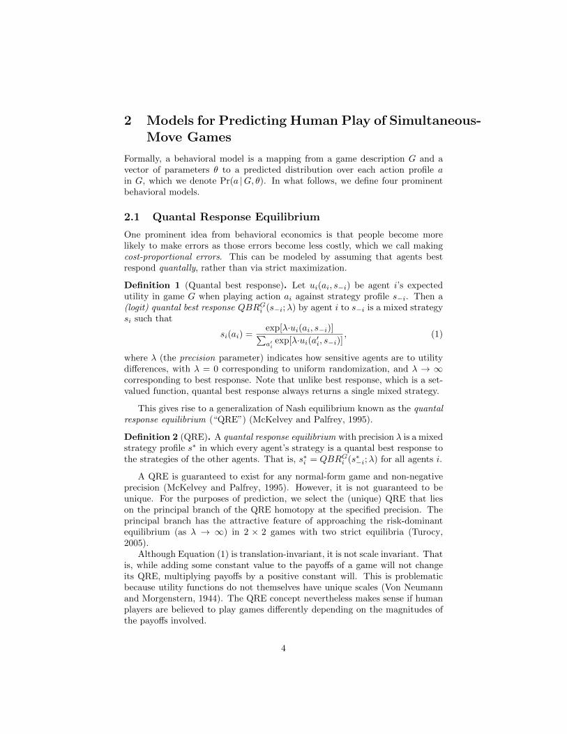
2 Models for Predicting Human Play of Simultaneous-Move Games
Formally, a behavioral model is a mapping from a game description G and avector of parameters θ to a predicted distribution over each action profile ain G, which we denote Pr(a |G, θ). In what follows, we define four prominentbehavioral models.
2.1 Quantal Response Equilibrium
One prominent idea from behavioral economics is that people become morelikely to make errors as those errors become less costly, which we call makingcost-proportional errors. This can be modeled by assuming that agents bestrespond quantally, rather than via strict maximization.
Definition 1 (Quantal best response). Let ui(ai, s−i) be agent i’s expectedutility in game G when playing action ai against strategy profile s−i. Then a(logit) quantal best response QBRGi (s−i;λ) by agent i to s−i is a mixed strategysi such that
si(ai) =exp[λ·ui(ai, s−i)]∑a′i
exp[λ·ui(a′i, s−i)], (1)
where λ (the precision parameter) indicates how sensitive agents are to utilitydifferences, with λ = 0 corresponding to uniform randomization, and λ → ∞corresponding to best response. Note that unlike best response, which is a set-valued function, quantal best response always returns a single mixed strategy.
This gives rise to a generalization of Nash equilibrium known as the quantalresponse equilibrium (“QRE”) (McKelvey and Palfrey, 1995).
Definition 2 (QRE). A quantal response equilibrium with precision λ is a mixedstrategy profile s∗ in which every agent’s strategy is a quantal best response tothe strategies of the other agents. That is, s∗i = QBRGi (s∗−i;λ) for all agents i.
A QRE is guaranteed to exist for any normal-form game and non-negativeprecision (McKelvey and Palfrey, 1995). However, it is not guaranteed to beunique. For the purposes of prediction, we select the (unique) QRE that lieson the principal branch of the QRE homotopy at the specified precision. Theprincipal branch has the attractive feature of approaching the risk-dominantequilibrium (as λ → ∞) in 2 × 2 games with two strict equilibria (Turocy,2005).
Although Equation (1) is translation-invariant, it is not scale invariant. Thatis, while adding some constant value to the payoffs of a game will not changeits QRE, multiplying payoffs by a positive constant will. This is problematicbecause utility functions do not themselves have unique scales (Von Neumannand Morgenstern, 1944). The QRE concept nevertheless makes sense if humanplayers are believed to play games differently depending on the magnitudes ofthe payoffs involved.
4

2.2 Level-k
Another key idea from behavioral economics is that humans can perform only alimited number of iterations of strategic reasoning.1 The level-k model (Costa-Gomes et al., 2001) captures this idea by associating each agent i with a levelki ∈ {0, 1, 2, . . .}, corresponding to the number of iterations of reasoning theagent is able to perform. A level-0 agent plays randomly, choosing uniformlyat random from his possible actions. A level-k agent, for k ≥ 1, best respondsto the strategy played by level-(k − 1) agents. If a level-k agent has more thanone best response, he mixes uniformly over them.
Here we consider a particular level-k model, dubbed Lk, which assumes thatall agents belong to levels 0,1, and 2.2 Each agent with level k > 0 has anassociated probability εk of making an “error”, i.e., of playing an action thatis not a best response to the level-(k − 1) strategy. Agents are assumed not toaccount for these errors when forming their beliefs about how lower-level agentswill act.
Definition 3 (Lk model). Let Ai denote player i’s action set, and BRGi (s−i)denote the set of i’s best responses in game G to the strategy profile s−i. LetIBRGi,k denote the iterative best response set for a level-k agent i, with IBRGi,0 =
Ai and IBRGi,k = BRGi (IBRG−i,k−1). Then the distribution πLki,k ∈ Π(Ai) thatthe Lk model predicts for a level-k agent i is defined as
πLki,0 (ai) = |Ai|−1,
πLki,k (ai) =
{(1− εk)/|IBRGi,k| if ai ∈ IBRGi,k,εk/(|Ai| − |IBRGi,k|) otherwise.
The overall predicted distribution of actions is a weighted sum of the distribu-tions for each level:
Pr(ai |G,α1, α2, ε1, ε2) =
2∑`=0
α`πLki,` (ai),
where α0 = 1 − α1 − α2. This model thus has 4 parameters: {α1, α2}, theproportions of level-1 and level-2 agents, and {ε1, ε2}, the error probabilities forlevel-1 and level-2 agents.
2.3 Cognitive Hierarchy
The cognitive hierarchy model (Camerer et al., 2004), like level-k, models agentswith heterogeneous bounds on iterated reasoning. It differs from the level-k model in two ways. First, agents do not make errors; each agent always
1This limit is generally believed to be quite low. For example, Arad and Rubinstein (2011)found no evidence for beliefs of fourth order or higher.
2We here model only level-k agents, unlike Costa-Gomes et al. (2001) who also modeledother decision rules.
5

best responds to its beliefs. Second, agents of level-m best respond to thefull distribution of agents at levels 0–m − 1, rather than only to level-(m − 1)agents. More formally, every agent has an associated level m ∈ {0, 1, 2, . . .}. Letf be a probability mass function describing the distribution of the levels in thepopulation. Level-0 agents play uniformly at random. Level-m agents (m ≥ 1)best respond to the strategies that would be played in a population describedby the truncated probability mass function f(j | j < m).
Camerer et al. (2004) advocate a single-parameter restriction of the cognitivehierarchy model called Poisson-CH, in which f is a Poisson distribution.
Definition 4 (Poisson-CH model). Let πPCHi,m ∈ Π(Ai) be the distribution overactions predicted for an agent i with level m by the Poisson-CH model. Letf(m) = Poisson(m; τ). Let BRGi (s−i) denote the set of i’s best responses ingame G to the strategy profile s−i. Let
πPCHi,0:m =
m∑`=0
f(`)πPCHi,`∑m`′=0 f(`′)
be the “truncated” distribution over actions predicted for an agent conditionalon that agent’s having level 0 ≤ ` ≤ m. Then πPCH is defined as
πPCHi,0 (ai) = |Ai|−1,
πPCHi,m (ai) =
{|BRGi (πPCHi,0:m−1)|−1 if ai ∈ BRGi (πPCHi,0:m−1),
0 otherwise.
The overall predicted distribution of actions is a weighted sum of the distribu-tions for each level:
Pr(ai |G, τ) =
∞∑`=0
f(`)πPCHi,` (ai).
The mean of the Poisson distribution, τ , is thus this model’s single parameter.
Rogers et al. (2009) argue that cognitive hierarchy predictions often exhibitcost-proportional errors (which they call the “negative frequency-payoff devia-tion relationship”), even though the cognitive hierarchy model does not explic-itly model this effect. This leaves open the question whether cognitive hierarchy(and level-k) predict well only to the extent that their predictions happen to ex-hibit cost-proportional errors, or whether bounded iterated reasoning capturesa distinct behavioral phenomenon.
2.4 Quantal Level-k
Stahl and Wilson (1994) propose a rich model of strategic reasoning that com-bines elements of the QRE and level-k models; we refer to it as the quantallevel-k model (QLk). In QLk, agents have one of three levels, as in Lk. Each
6

agent responds to its beliefs quantally, as in QRE. Like Lk, each agent believesthat the rest of the population has the next-lower type.
A key difference between QLk and Lk is in the error structure. In Lk, higher-level agents believe that all lower-level agents best respond perfectly, although infact every agent has some probability of making an error. In contrast, in QLk,agents are aware of the quantal nature of the lower-level agents’ responses,and have a (possibly incorrect) belief about the lower-level agents’ precision.That is, level-1 and level-2 agents use potentially different precisions (λ’s), andfurthermore level-2 agents’ beliefs about level-1 agents’ precision can be wrong.
Definition 5 (QLk model). The probability distribution πQLki,k ∈ Π(Ai) overactions that QLk predicts for a level-k agent i is
πQLki,0 (ai) = |Ai|−1,
πQLki,1 = QBRGi (πQLk−i,0 ;λ1),
πQLki,1(2) = QBRGi (πQLk−i,0 ;λ1(2)),
πQLki,2 = QBRGi (πQLki,1(2);λ2),
where πQLki,1(2) is a mixed-strategy profile representing level-2 agents’ (possibly in-
correct) beliefs about how level-1 agents play. The overall predicted distributionof actions is the weighted sum of the distributions for each level:
Pr(ai |α1, α2, λ1, λ2, λ1(2)) =
2∑k=0
αkπQLki,k (ai),
where α0 = 1−α1−α2. The QLk model thus has five parameters: {α1, α2, λ1, λ2, λ1(2)}.
3 Methods I: Comparing Models
3.1 Prediction Framework
How do we determine whether a behavioral model is well supported by experi-mental data? Formally, a behavioral model is a mapping from a game descrip-tion G and a vector of parameters θ to a predicted distribution over each actionprofile a in G, which we denote Pr(a |G, θ). Assume that there is some “true”set of parameter values, θ∗, under which the model outputs the true distributionPr(a |G) over action profiles, and that θ is independent of G. An experimentaldataset, D, is a set of elements (Gi, ai), where Gi is a game and ai is a (pure)action played by a human player in Gi. (Observe that there is no reason topair the play of a human player with that of his opponent, as games are unre-peated.) Our model can only be used to make predictions when its parametersare instantiated.
We use the maximum likelihood estimate of the parameters based on D,
θ = arg maxθ
Pr(D | θ),
7

as a point estimate of the true set of parameters θ∗. We then use θ to evaluatethe model:
Pr(a |G,D) = Pr(a |G, θ). (2)
The likelihood of a single datapoint di = (Gi, ai) ∈ D is
Pr(di | θ) = Pr(Gi, ai | θ).
By the chain rule of probabilities, this is equivalent to
Pr(di | θ) = Pr(ai |Gi, θ) Pr(Gi | θ),
and by independence of G and θ we have
Pr(di | θ) = Pr(ai |Gi, θ) Pr(Gi). (3)
The datapoints are independent, so the likelihood of the dataset is just theproduct of the likelihoods of the datapoints,
Pr(D | θ) =∏di∈D
Pr(ai |Gi, θ) Pr(Gi). (4)
The probabilities Pr(Gi) are constant with respect to θ, and can therefore bedisregarded when maximizing the likelihood:
arg maxθ
Pr(D | θ) = arg maxθ
∏di∈D
Pr(ai |Gi, θ).
3.2 Assessing generalization performance
We evaluate a given model on a given dataset by the (log) likelihood ; that is,by how probable the test data is according to the model. That is, the moreprobable the observed data according to the model, the better we say that themodel predicted the data. We used the maximum likelihood estimate for eachmodels parameters on disjoint training data.
Randomly dividing our experimental data into training and test sets in-troduces variance into the prediction score, since the exact value of the scoredepends partly upon the random division. To reduce this variance, we perform10 rounds of 10-fold cross-validation. Specifically, for each round, we randomlydivide the dataset into 10 equal-sized parts. For each of the 10 ways of selecting9 parts from the 10, we compute the maximum likelihood estimate of the model’sparameters based on those 9 parts. We then determine the log likelihood of theremaining part given the prediction. We call the average of this quantity acrossall 10 parts the cross-validated log likelihood. The average (across rounds) of thecross-validated log likelihoods is distributed according to a Student’s-t distribu-tion (see, e.g., Witten and Frank, 2000). We compare the predictive power ofdifferent behavioral models on a given dataset by comparing the average cross-validated log likelihood of the dataset under each model. We say that one modelpredicts significantly better than another when the 95% confidence intervals forthe average cross-validated log likelihoods do not overlap.
8
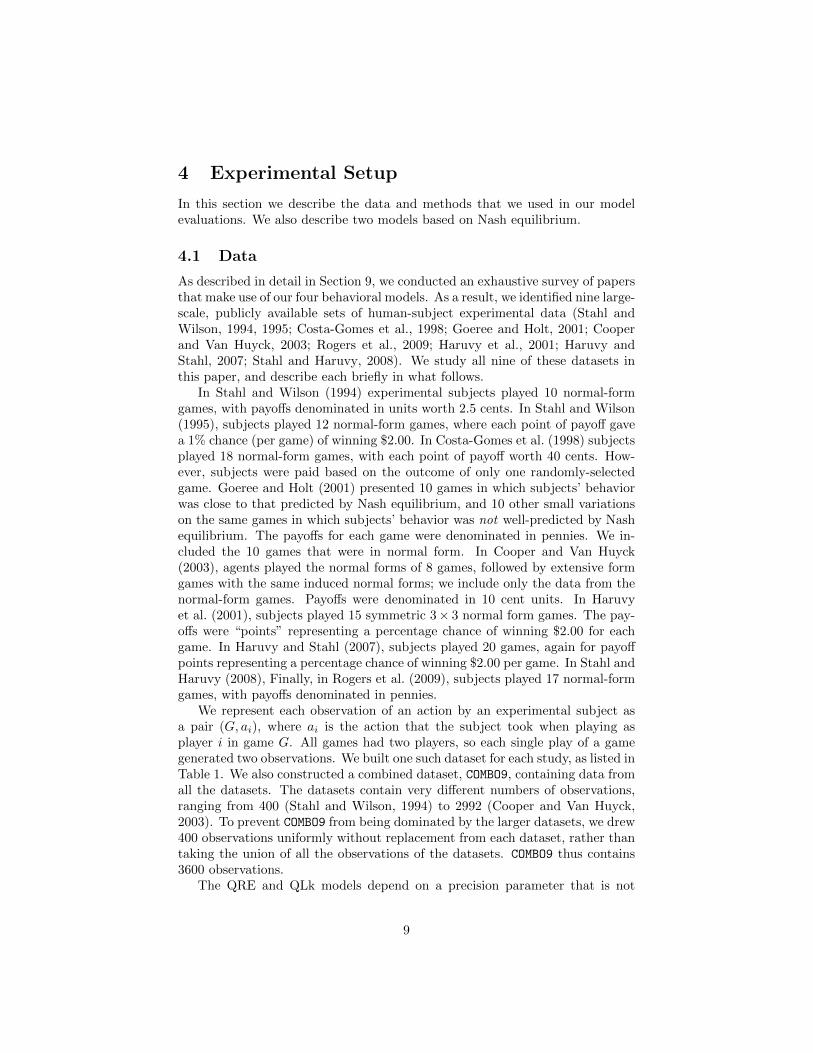
4 Experimental Setup
In this section we describe the data and methods that we used in our modelevaluations. We also describe two models based on Nash equilibrium.
4.1 Data
As described in detail in Section 9, we conducted an exhaustive survey of papersthat make use of our four behavioral models. As a result, we identified nine large-scale, publicly available sets of human-subject experimental data (Stahl andWilson, 1994, 1995; Costa-Gomes et al., 1998; Goeree and Holt, 2001; Cooperand Van Huyck, 2003; Rogers et al., 2009; Haruvy et al., 2001; Haruvy andStahl, 2007; Stahl and Haruvy, 2008). We study all nine of these datasets inthis paper, and describe each briefly in what follows.
In Stahl and Wilson (1994) experimental subjects played 10 normal-formgames, with payoffs denominated in units worth 2.5 cents. In Stahl and Wilson(1995), subjects played 12 normal-form games, where each point of payoff gavea 1% chance (per game) of winning $2.00. In Costa-Gomes et al. (1998) subjectsplayed 18 normal-form games, with each point of payoff worth 40 cents. How-ever, subjects were paid based on the outcome of only one randomly-selectedgame. Goeree and Holt (2001) presented 10 games in which subjects’ behaviorwas close to that predicted by Nash equilibrium, and 10 other small variationson the same games in which subjects’ behavior was not well-predicted by Nashequilibrium. The payoffs for each game were denominated in pennies. We in-cluded the 10 games that were in normal form. In Cooper and Van Huyck(2003), agents played the normal forms of 8 games, followed by extensive formgames with the same induced normal forms; we include only the data from thenormal-form games. Payoffs were denominated in 10 cent units. In Haruvyet al. (2001), subjects played 15 symmetric 3× 3 normal form games. The pay-offs were “points” representing a percentage chance of winning $2.00 for eachgame. In Haruvy and Stahl (2007), subjects played 20 games, again for payoffpoints representing a percentage chance of winning $2.00 per game. In Stahl andHaruvy (2008), Finally, in Rogers et al. (2009), subjects played 17 normal-formgames, with payoffs denominated in pennies.
We represent each observation of an action by an experimental subject asa pair (G, ai), where ai is the action that the subject took when playing asplayer i in game G. All games had two players, so each single play of a gamegenerated two observations. We built one such dataset for each study, as listed inTable 1. We also constructed a combined dataset, COMBO9, containing data fromall the datasets. The datasets contain very different numbers of observations,ranging from 400 (Stahl and Wilson, 1994) to 2992 (Cooper and Van Huyck,2003). To prevent COMBO9 from being dominated by the larger datasets, we drew400 observations uniformly without replacement from each dataset, rather thantaking the union of all the observations of the datasets. COMBO9 thus contains3600 observations.
The QRE and QLk models depend on a precision parameter that is not
9

Table 1: Names and contents of each dataset. Units are in expected value.
Source Games Observations Units
Stahl and Wilson (1994) 10 400 $0.025Stahl and Wilson (1995) 12 576 $0.02Costa-Gomes et al. (1998) 18 1566 $0.022Goeree and Holt (2001) 10 500 $0.01Cooper and Van Huyck (2003) 8 2992 $0.10Rogers et al. (2009) 17 1210 $0.01Haruvy et al. (2001) 15 869 $0.02Haruvy and Stahl (2007) 20 2940 $0.02Stahl and Haruvy (2008) 18 1288 $0.02
COMBO9 128 3600 $0.01
scale-invariant. That is, if λ is the correct value for a game whose payoffs aredenominated in cents, then λ/100 would be the correct value for a game whosepayoffs are denominated in dollars. To ensure consistent estimation of precisionparameters, especially in the COMBO9 dataset where observations from multiplestudies are combined, we normalized the payoff values for each game to be inexpected cents.3
4.2 Comparing to Nash Equilibrium
It is desirable to compare the predictive performance of our behavioral modelsto that of Nash equilibrium. However, such a comparison is not as simple asone might hope, because any attempt to use Nash equilibrium for predictionmust extend the solution concept to solve two problems. The first problemis that many games have multiple Nash equilibria; in these cases, the Nash“prediction” is not well defined. The second problem is that Nash equilibriumfrequently assigns probability zero to some actions. Indeed, in 72% of the gamesin our COMBO9 dataset every Nash equilibrium assigned probability 0 to actionsthat were actually taken by experimental subjects. This is a problem becausewe assess the quality of a model by how well it explains the data; unmodified,Nash equilibrium model considers our experimental data to be impossible, andhence receives a log likelihood of negative infinity.4
3As described earlier, in some datasets, payoff points were worth a certain number of cents;in others, points represented percentage chances of winning a certain sum, or were otherwisein “expected” units. Table 1 lists the number of expected cents that we deemed each payoffpoint to be worth for the purposes of normalization.
4One might wonder whether the ε-equilibrium solution concept solves either of these prob-lems. It does not: ε-equilibrium can still assign probability 0 to some actions, and relaxing theequilibrium concept only increases the number of equilibria. Indeed, every game has infinitelymany ε-equilibria for any ε > 0. To our knowledge, no algorithm for characterizing this setexists, making equilibrium selection impractical. Thus, we did not consider ε-equilibrium in
10

We addressed the second problem by augmenting the Nash equilibrium so-lution concept to say that with some probability, each player chooses an actionuniformly at random. This probability is thus a free parameter of the model; aswe did with behavioral models, we fit this parameter using maximum likelihoodestimation on a training set. (We thus call the model Nash Equilibrium withError, or NEE.) We sidestepped the first problem, assuming that agents alwayscoordinate to some equilibrium, and reporting statistics across different equilib-ria, in some cases “cheating” by looking at the test set. Specifically, we reportthe performance achieved by choosing the equilibria that respectively best andworst fit the test data, thereby giving upper and lower bounds on the test-setperformance of any Nash-based prediction. We also report the expected predic-tion performance achieved by randomly sampling a Nash equilibrium uniformlyat random and assuming that agents play this equilibrium; observe that thismodel can be evaluated without looking at the test set (“cheating”).
4.3 Computational Environment
We performed computation on the glacier, hermes, and orcinus clusters ofWestGrid (www.westgrid.ca), which have 1680 32-bit Intel Xeon CPU cores,672 64-bit Intel Xeon CPU cores, and 9600 64-bit Intel Xeon CPU cores, re-spectively. In total, computing the results reported in this paper required over aCPU-year of machine time, primarily for model fitting and posterior estimation.Specifically, we used Gambit (McKelvey et al., 2007) to compute QRE and toenumerate the Nash equilibria of games, and computed maximum likelihoodestimates using the Nelder–Mead simplex algorithm (Nelder and Mead, 1965).
5 Model Comparisons
In this section we describe the results of our experiments comparing the pre-dictive performance of the four behavioral models from Section 2 and of theNash-based models of Section 4.2. Figure 1 compares our behavioral and Nash-based models. For each model and each dataset, we give the factor by whichthe dataset is more likely according to the model’s prediction than it is accord-ing to a uniform random prediction. Thus, for example, the COMBO9 datasetis approximately 1018 times more likely according to Poisson-CH’s predictionthan it is according to a uniform random prediction. For the Nash Equilibriumwith Error model, the error bars show the upper and lower bounds on predictiveperformance obtained by selecting an equilibrium so as to maximize or minimizetest-set performance, and the bar shows the expected predictive performance ofselecting an equilibrium uniformly at random.
our study.
11

100
1010
1020
1030
1040
1050
1060
COMBO9
SW94SW95
CGCB98
GH01HSW01
CVH03
RPC09
HS07SH08
Like
lihoo
d im
prov
emen
tQRE
Poisson-CHLk
QLkNEE
Figure 1: Average likelihood ratios of model predictions to random predictions,with 95% confidence intervals. Confidence intervals for NEE range over equilib-ria as well as fold partitions.
5.1 Comparing Behavioral Models
In six datasets, including COMBO9, the model based on cost-proportional errors(QRE) predicted human play significantly better than the two models based onbounded iterated reasoning (Lk and Poisson-CH). However, in four datasets,the situation was reversed, with Lk and Poisson-CH outperforming QRE. Thismixed result is consistent with earlier comparisons of QRE with these two mod-els (Chong et al., 2005; Crawford and Iriberri, 2007; Rogers et al., 2009), andsuggests to us that bounded iterated reasoning and cost-proportional errorscapture distinct underlying phenomena. If this claim is true, we might expectthat our remaining model, which incorporates both components, would predictbetter than models that incorporate only one component. This was indeed thecase: QLk generally outperformed the single-component models. Overall, QLkwas the strongest of the behavioral models, predicting significantly better thanall models in all datasets except CVH03 and SW95 (and GH01, which we discussin detail below).
Earlier studies found relatively few level-0 agents. Stahl and Wilson (1994)estimated 0% of the population were level-0; Stahl and Wilson (1995) estimated17%, with a confidence interval of [6%, 30%]; and Haruvy et al. (2001) estimatedrates between 6–16% for various model specifications. In contrast, our fittedparameters for the Lk and QLk models estimated large proportions of level-0agents (56% and 38% respectively on the COMBO9 dataset). This is explained by
12

100
105
1010
1015
1020
GH01Treasure
Contradiction
Like
lihoo
d im
prov
emen
t
QREPoisson-CH
LkQLkNEE
Figure 2: Average likelihood ratios of model predictions to random predictions,with 95% confidence intervals, on GH01 data separated into “treasure” and “con-tradiction” treatments. Confidence intervals for NEE range over equilibria aswell as fold partitions.
differences in the fitting procedures used. We chose parameters to maximize thecombined likelihood of each action/game pair observation, treating the agentsas anonymous, whereas the cited studies maximized the combined likelihoods ofper-subject sequences of choices. We analyze the full distributions of parametervalues in Section 7.
5.2 Comparing to Nash Equilibrium
It is already widely believed that Nash equilibrium is a poor description of hu-mans’ initial play in normal-form games (e.g., see Goeree and Holt, 2001). Nev-ertheless, for the sake of completeness, we also evaluated the predictive powerof Nash equilibrium with error on our datasets. Referring again to Figure 1,we see that NEE’s predictions were worse than those of every behavioral modelon every dataset except SW95. NEE’s predictions were significantly worse thanthose of QLk on every dataset except SW95 and GH01.
We found NEE’s strong performance on SW95 to be surprising; we believethat this finding may warrant additional study. In contrast, it is unsurprisingthat NEE performed well on GH01, since this distribution was deliberately con-structed so that human play on half of its games (the “treasure” conditions)would be relatively well-described by Nash equilibrium. Figure 2 separatesGH01 into its “treasure” and “contradiction” treatments and compares the per-formance of the BGT and Nash-based models on these separated datasets. Notethat although NEE had a higher upper bound than QLk on the “treasure” treat-ment, its expected performance was still substantially worse than most of theBGT models.
In addition to the deliberate selection of “treasures”, many of GH01’s gameshave multiple equilibria, which offers an advantage to our NEE model’s upperbound (because it gets to pick the equilibrium with best test-set performanceon a per-instance basis); see Section 5.3 below.
13

Table 2: Datasets separated by game features. The column headed “games”indicates how many games of the full dataset meet the criterion, and the col-umn headed “n” indicates how many observations each feature-based datasetcontains.
Name Description Games n
D1 Weak dominance solvable in one round 2 748D2 Weak dominance solvable in two rounds 38 5058D2s Strict dominance solvable in two rounds 23 2000DS Weak dominance solvable 44 5446DSs Strict dominance solvable 28 2338ND Not weak dominance solvable 84 6625
PSNE1 Single Nash equilibrium, which is pure 42 4431MSNE1 Single Nash equilibrium, which is mixed 24 2509Multi-Eqm Multiple Nash equilibria 62 5131
5.3 Dataset Composition
As we have already seen in the case of GH01, our experimental results are sensi-tive to choices made by the authors of our various datasets about which gamesto include. In this section we describe how features of these games influencedmodel performance. In particular, we divided the combined dataset based onfeatures of the games and evaluated models fit on each subset.
Overall, our datasets spanned 128 games. The vast majority of these gamesare matrix games, deliberately lacking inherent meaning in order to avoid fram-ing effects. (Indeed, some studies (e.g., Rogers et al., 2009) even avoid “focal”payoffs like 0 and 100.) For the most part, these games were chosen to varyaccording to dominance solvability and equilibrium structure. In particular,authors were concerned with whether a game could be solved by iterated re-moval of dominated strategies (either strict or weak), and with how many stepsof iteration were required; and with the number and type of Nash equilibriathat each game possesses. The two exceptions are Goeree and Holt (2001),who chose games which had both intuitive equilibria and strategically equiv-alent variations with counterintuitive equilibria; and Cooper and Van Huyck(2003), whose normal form games were based on an exhaustive enumeration ofthe payoff orderings possible in generic 2-player, 2-action extensive-form games.
We constructed subsets of the full dataset based on these criteria as describedin Table 2.5 We used the full dataset with no subsampling rather than Combo9,as there is less concern about one study dominating a dataset that has beenfiltered to contain games of a specific type.
We computed cross-validated MLE fits for each model on each of the feature-based datasets of Table 2. The results are summarized in Figure 3. In two
5These criteria are not all mutually exclusive, so the total number of games does not sumto 128.
14

respects, the results across the feature-based datasets mirror the results of Sec-tion 5.1 and Section 5.2. First, QLk significantly outperformed the other be-havioral models on almost every dataset; the sole exception is D1, where QLkperformed insignificantly better than Lk. Second, every behavioral model sig-nificantly outperformed NEE in all but three datasets: D1, ND and Multi-eqm.In these three datasets, the upper and lower bounds on NEE’s performancecontain the performance of either two or all three of the single-factor behav-ioral models (but not QLk). The performance of all models on the D1 datasetis roughly similar, likely due to the ease with which various different forms ofreasoning can uncover a dominant strategy. It is unsurprising that NEE’s up-per and lower bounds would be widely separated on the Multi-eqm dataset,since the more equilibria a game has, the more likely it is that there will existan equilibrium that fits well post-hoc. It turns out that 55 of the 84 games(and 4731 of the 6625 observations) in the ND dataset are from the Multi-eqm
dataset, which likely explains NEE’s high upper bound in that dataset as well.Indeed, this analysis helps to explain some of our previous observations aboutthe GH01 dataset. NEE contains all other models in its performance boundsin this dataset, and in addition to the fact that half the dataset’s games (the“treasure” treatments) that were chosen for consistency with Nash equilibrium,some of the other games (the “contradiction” treatments) turn out to have mul-tiple equilibria. Overall, the overlap between GH01 and Multi-eqm is 5 gamesout of 10, and 250 observations out of 500.
Unlike in the per-dataset comparisons of Section 5.1, both iterative single-factor models (Poisson-CH and Lk) significantly outperformed QRE in everyfactor-based dataset. One possible explanation is that the filtering factors areall biased toward iterative models. However, it seems unlikely that, e.g., bothdominance-solvability and dominance-nonsolvability are biased toward iterativemodels. Another possibility is that iterative models are a better model of humanbehavior, but the cost-proportional error model of QRE is sufficiently superiorto the respectively simple and non-existent error models of Poisson-CH and Lkthat it outperforms on many datasets that mix game types. Or, similarly, iter-ative models may fit very differently on dominance solvable and non-dominancesolvable games; in this case, they would perform very poorly on mixed data.
6 Methods II: Analyzing Model Parameters
Using BGT models to make good predictions about human behavior requiresusing “good” estimates of the model parameters. However, these estimates canalso be useful in themselves. Examining parameter values that perform well canhelp researchers understand both how people behave in strategic situations andwhether a model’s behavior aligns or clashes with its intended economic inter-pretation. However, the maximum likelihood estimation of Section 3—findinga single set of parameters that best explains the training set—is not a goodway of gaining this kind of understanding. The problem is that we have no wayof knowing how much of a difference it would have made to have set the pa-
15

100105
101010151020102510301035
Like
lihoo
d im
prov
emen
t
DS (n=5446)100101102103104105
D1 (n=748)100105
10101015102010251030
D2 (n=5058)
QREPCH
LkQLkNEE
100102104106108
10101012101410161018
Like
lihoo
d im
prov
emen
t
DSS (n=2338)100102104106108
101010121014
D2S (n=2000)100
10101020103010401050106010701080
ND (n=6625)
100105
10101015102010251030
Like
lihoo
d im
prov
emen
t
PSNE1 (n=4431)100102104106108
1010101210141016
MSNE1 (n=2509)100
1010102010301040105010601070
Multi-Eqm (n=5131)
Figure 3: Average likelihood ratios of model predictions to random predictions,with 95% confidence intervals, on feature-based datasets. Confidence intervalsfor NEE range over equilibria as well as fold partitions.
rameters differently, and hence how important each parameter setting is to themodel’s performance. For example, if some parameter is completely uncorre-lated with predictive accuracy, the maximum likelihood estimate will set it to anarbitrary value, from which we would be wrong to draw economic conclusions.Similarly, if there are multiple, very different ways of configuring the model tomake good predictions, we would not want to draw firm conclusions about howpeople reason. An alternative is to use Bayesian analysis to estimate the entireposterior distribution over parameter values, rather than simply estimating themode of this distribution. This allows us to identify the most likely parametervalues; how wide a range of values are argued for by the data (equivalently, howstrongly the data argues for the most likely values); and whether the values thatthe data argues for are plausible in terms of our intuitions about parameters’meanings. In this section we derive an expression for the posterior distribution,and describe methods for constructing posterior estimates and using them toassess parameter importance. In Section 7 we will apply these methods to studyQLk and Poisson-CH: the former because it achieved such reliably strong per-formance, and the latter because it is the model about which the most explicitparameter recommendation was made in the literature.
16
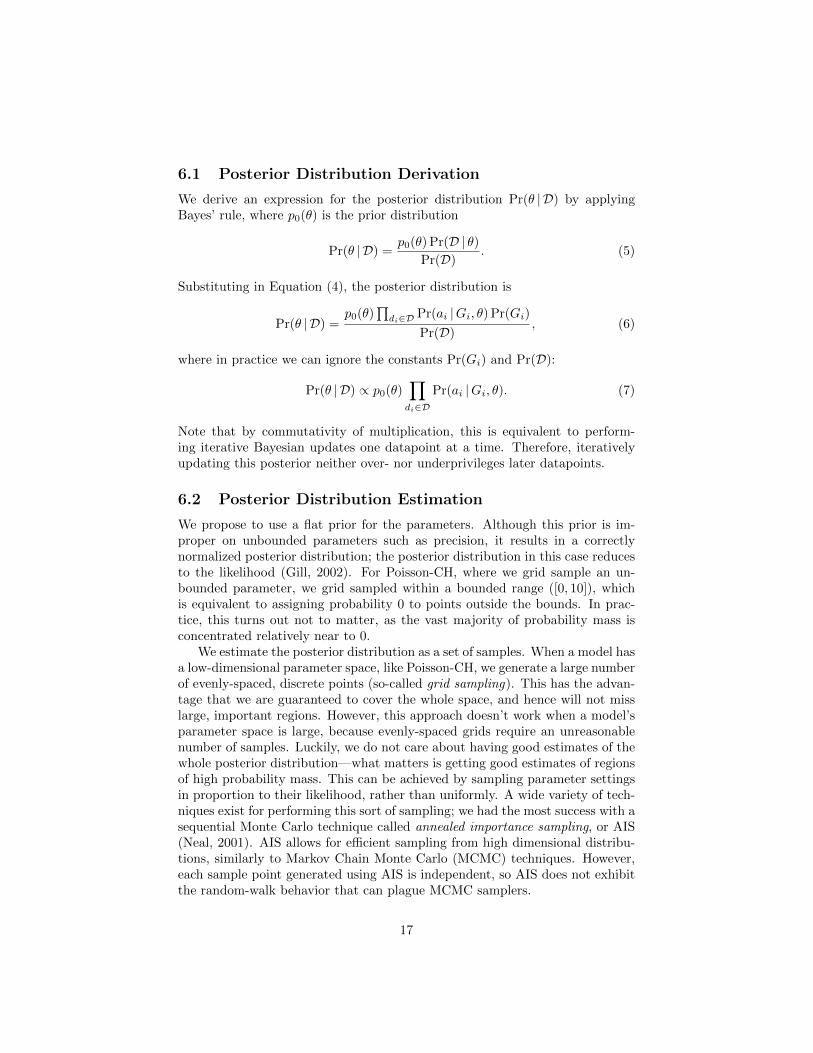
6.1 Posterior Distribution Derivation
We derive an expression for the posterior distribution Pr(θ | D) by applyingBayes’ rule, where p0(θ) is the prior distribution
Pr(θ | D) =p0(θ) Pr(D | θ)
Pr(D). (5)
Substituting in Equation (4), the posterior distribution is
Pr(θ | D) =p0(θ)
∏di∈D Pr(ai |Gi, θ) Pr(Gi)
Pr(D), (6)
where in practice we can ignore the constants Pr(Gi) and Pr(D):
Pr(θ | D) ∝ p0(θ)∏di∈D
Pr(ai |Gi, θ). (7)
Note that by commutativity of multiplication, this is equivalent to perform-ing iterative Bayesian updates one datapoint at a time. Therefore, iterativelyupdating this posterior neither over- nor underprivileges later datapoints.
6.2 Posterior Distribution Estimation
We propose to use a flat prior for the parameters. Although this prior is im-proper on unbounded parameters such as precision, it results in a correctlynormalized posterior distribution; the posterior distribution in this case reducesto the likelihood (Gill, 2002). For Poisson-CH, where we grid sample an un-bounded parameter, we grid sampled within a bounded range ([0, 10]), whichis equivalent to assigning probability 0 to points outside the bounds. In prac-tice, this turns out not to matter, as the vast majority of probability mass isconcentrated relatively near to 0.
We estimate the posterior distribution as a set of samples. When a model hasa low-dimensional parameter space, like Poisson-CH, we generate a large numberof evenly-spaced, discrete points (so-called grid sampling). This has the advan-tage that we are guaranteed to cover the whole space, and hence will not misslarge, important regions. However, this approach doesn’t work when a model’sparameter space is large, because evenly-spaced grids require an unreasonablenumber of samples. Luckily, we do not care about having good estimates of thewhole posterior distribution—what matters is getting good estimates of regionsof high probability mass. This can be achieved by sampling parameter settingsin proportion to their likelihood, rather than uniformly. A wide variety of tech-niques exist for performing this sort of sampling; we had the most success with asequential Monte Carlo technique called annealed importance sampling, or AIS(Neal, 2001). AIS allows for efficient sampling from high dimensional distribu-tions, similarly to Markov Chain Monte Carlo (MCMC) techniques. However,each sample point generated using AIS is independent, so AIS does not exhibitthe random-walk behavior that can plague MCMC samplers.
17

Briefly, the annealed importance sampling procedure is as follows. A sample#»
θ 0 is drawn from an easy-to-sample-from distribution P0. For each Pj in asequence of intermediate distributions P1, . . . , Pr−1 that become progressivelycloser to the posterior distribution, a sample
#»
θ j is generated by drawing a sam-
ple#»
θ ′ from a proposal distribution Q(· | #»
θ j−1), and accepted with probability
Pj(#»
θ ′)Q(#»
θ j−1 |#»
θ ′)
Pj(#»
θ j−1)Q(#»
θ ′ | #»
θ j−1). (8)
If the proposal is accepted,#»
θ j =#»
θ ′; otherwise,#»
θ j =#»
θ j−1. We repeat thisprocedure multiple times, obtaining one sample each time. In the end, ourestimate of the posterior is the set of
#»
θ r values, each weighted according to
P1(#»
θ 0)P2(#»
θ 1)
P0(#»
θ 0)P1(#»
θ 1)· · · Pr−1(
#»
θ r−2)Pr(#»
θ r−1)
Pr−2(#»
θ r−2)Pr−1(#»
θ r−1). (9)
7 Bayesian analysis of model parameters
In this section we analyze the posterior distributions of the parameters for twoof the models compared in Section 5: Poisson-CH and QLk. We computed allposterior distributions with respect to the COMBO9 dataset. For Poisson-CH, wecomputed the likelihood for each value of τ ∈ {0.01k | k ∈ N, 0 ≤ 0.01k ≤ 10},and then normalized by the sum of the likelihoods. For QLk, we used annealedimportance sampling. For the initial sampling distribution P0, we used a prod-uct distribution over the population proportions parameters and the precisionparameters. For the population proportion parameter components we used aDirichlet distribution Dir(1, 1, 1); this is equivalent to uniformly sampling overthe simplex of all possible combinations of population proportions. For theprecision parameter components we used the renormalized non-negative half ofa univariate Gaussian distribution N (0, 22) for each precision parameter; thisgives a distribution that is decreasing in precision (on the assumption thathigher precisions are less likely than lower ones), and with a standard devia-tion of 2, which was large enough to give a non-negligible probability to mostprevious precision estimates. For the proposal distribution, we chose a prod-uct distribution “centered” at the current value, with proportion parameters#»α ′ sampled from Dir(20 #»αj−1), and each precision parameter λ′ sampled fromN (λj−1, 0.2
2) (truncated at 0 and renormalized). We chose the “hyperparame-ters” for the Dirichlet distribution (20) and the precision distributions (0.22) bytrial and error on a small subset of the data to make the acceptance rate nearto the standard heuristic value of 0.5 (Robert and Casella, 2004). We used 200intermediate distributions of the form
Pj(#»
θ ) = Pr(#»
θ | D)γj ,
with the first 40 γj ’s spaced uniformly from 0 to 0.01, and the remaining 160 γj ’sspaced geometrically from 0.01 to 1, as in the original AIS description (Neal,
18

0
0.2
0.4
0.6
0.8
1
0 0.5 1 1.5 2
Cum
ulat
ive
prob
abilit
y
τ
COMBO9SW94SW95
CGCB98GH01
HSW01CVH03RPC09
HS07SH08
Figure 4: Cumulative posterior distributions for the τ parameter of the Poisson-CH model. Bold trace is for the combined dataset; solid trace is for the out-lier Stahl and Wilson (1994) source dataset; dotted traces are all other sourcedatasets.
2001). We performed 5 Metropolis updates in each distribution before movingto the next distribution in the chain.
7.1 Poisson-CH
Camerer et al. (2004) recommend setting the τ parameter of the Poisson-CHmodel to 1.5. Figure 4 gives the cumulative posterior distribution over τ foreach of our datasets. Overall, our analysis strongly contradicts Camerer et al.’srecommendation. On COMBO9, the posterior probability of 0.51 ≤ τ ≤ 0.59 ismore than 99%. Every other source dataset had a wider 99% credible interval(a Bayesian counterpart to confidence interval) for τ than COMBO9, as indicatedby the higher slope of COMBO9’s cumulative density function; this is expected, assmaller datasets lead to less confident predictions. Nevertheless, all but two ofthe source datasets had median values less than 1.0. Only the Stahl and Wilson(1994) dataset (SW94) appears to support Camerer et al.’s recommendation (me-dian 1.43). However, SW94 appears to be an outlier; its credible interval is widerthan that of the other distributions, and the distribution is very multimodal,likely due to SW94’s small size.
7.2 QLk
Figure 5 gives the marginal cumulative posterior distributions for each of theparameters of the QLk model. (That is, we computed the five-dimensional pos-terior distribution, and then extracted from it the five marginal distributionsshown here.) We found these distributions surprising for several reasons. First,the models predict many more level-2 agents than level-1 agents. In contrast, itis typically assumed that higher level agents are scarcer, as they perform morecomplex strategic reasoning. Even more surprisingly, the model predicts thatlevel-1 agents should have much higher precisions than level-2 agents. This isodd if the level-2 agents are to be understood as “more rational”; indeed, preci-
19

0
0.2
0.4
0.6
0.8
1
0 0.1 0.2 0.3 0.4 0.5
Cum
ulat
ive
prob
abilit
yLevel proportions
α1α2
0
0.2
0.4
0.6
0.8
1
0 0.5 1 1.5 2 2.5 3 3.5 4
Cum
ulat
ive
prob
abilit
y
Precisions
λ1λ2λ1(2)
Figure 5: Marginal cumulative posterior distribution functions for the level pro-portion parameters (α1, α2; top panel) and precision parameters (λ1, λ2, λ1(2);bottom panel) of the QLk model on the combined dataset.
sion is sometimes interpreted as a measure of rationality (e.g., see Weizsacker,2003; Gao and Pfeffer, 2010). Third, the distribution of λ1(2), the precision thatlevel-2 agents ascribe to level-1 agents, is very concentrated around very smallvalues ([0.023, 0.034]). This differs by two orders of magnitude from the “true”value of λ1, which is quite concentrated around its median value of 3.1. Finally,disregarding the ordering of λ1 and λ2, the median value of λ1 (3.1) is morethan 17 times larger than that of λ2 (0.18). It seems unlikely that level-1 agentswould be an order of magnitude more sensitive to utility differences than level-2agents.
One interpretation is that the QLk model is essentially accurate, and theseparameter values simply reflect a surprising reality. For example, the low preci-sion of level-2 agents and the even lower precision that they (incorrectly) ascribeto the level-1 agents may indicate that two-level strategic reasoning causes a highcognitive load, which makes agents more likely to make mistakes, both in theirown actions and in their predictions. The main appeal of this explanation isthat it allows us to accept the QLk model’s strong performance at face value.
An alternate interpretation is that QLk fails to capture some crucial aspectof experimental subjects’ strategic reasoning. For example, if the higher-levelagents reasoned about all lower levels rather than only one level below them-selves, then the low value of λ1(2) could predict well because it “simulates” amodel where level-2 agents respond to a mixture of level-0 and level-1 agents.We investigate this second possibility in the next section.
20

8 Model Variations
In this section, we investigate the properties of the QLk model by evaluatingthe predictive power of a family of systematic variations of the model. In theend, we identify a simpler model that dominates QLk on our data, and whichalso yields much more reasonable marginal distributions over parameter values.
Specifically, we constructed a family of models by extending or restrictingthe QLk model along four different axes. QLk assumes a maximum level of2; we considered maximum levels of 1 and 3 as well. QLk has inhomogeneousprecisions in that it allows each level to have a different precision; we variedthis by also considering homogeneous precision models. QLk allows general pre-cision beliefs that can differ from lower level agents’ true precisions; we alsoconstructed models that make the simplifying assumption that all agents haveaccurate precision beliefs. Finally, in addition to Lk beliefs, where all otheragents are assumed by a level-k agent to be level-(k − 1), we also constructedmodels with CH beliefs, where agents believe that the population consists ofthe true, truncated distribution over the lower levels. We evaluated each com-bination of axis values; the 17 resulting models6 are listed in the top part ofTable 3. In addition to the 17 exhaustive axis combinations for models with max-imum levels in {1, 2, 3}, we also evaluated 12 additional axis combinations thathave higher maximum levels and 8 parameters or fewer: ai-QCH4 and ai-QLk4;ah-QCH and ah-QLk variations with maximum levels in {4, 5, 6, 7}; and ah-QCH
and ah-QLk variations that assume a Poisson distribution over the levels ratherthan using an explicit tabular distribution.7 These additional models are listedin the bottom part of Table 3.
8.1 Simplicity Versus Predictive Performance
We evaluated the predictive performance of each model on the COMBO9 datasetusing 10-fold cross-validation repeated 10 times, as in Section 5. The results aregiven in the last column of Table 3 and plotted in Figure 6.
All else being equal, a model with higher performance is more desirable,as is a model with fewer parameters. We can plot an “efficient frontier” ofthose models that achieved the (statistically significantly) best performance fora given number of parameters or fewer; see Figure 6. The original QLk model(gi-QLk2) is not efficient in this sense; it is dominated by ah-QCH3, which hassignificantly better predictive performance even though it has fewer parame-ters (due to restricting agents to homogeneous precisions and accurate beliefs).Our analysis thus argues that the flexibility added by inhomogeneous precisionsand general precision beliefs is less important than the number of levels andthe choice of population belief. Conversely, the poor performance of the Pois-son variants relative to ah-QCH3 suggests that flexibility in describing the leveldistribution is more important than the total number of levels modeled.
6When the maximum level is 1, all combinations of the other axes yield identical predic-tions. Therefore there are only 17 models instead of 3 · 23 = 24.
7The ah-QCHp model is equivalent to the CH-QRE model of Camerer et al. (2011).
21

1026
1027
1028
1029
1030
1031
1 2 3 4 5 6 7 8 9 10 11
Like
lihoo
d im
prov
emen
t ove
r u.a
.r.
Number of parameters
Model performanceEfficient frontier
gi-QLk
ai-QLk2
gh-QLk2
ah-QLk2
gi-QCH2
ai-QCH2
gh-QCH2
ah-QCH2
gi-QLk3
ai-QLk3
gh-QLk3
ah-QLk3
gi-QCH3
ai-QCH3
ah-QLk4ah-QLk5 ah-QLk6
ah-QCH6
ah-QLk7
ah-QCH7
ah-QLkp
gh-QCH3
ah-QCHp
ah-QCH3
ah-QCH4
ah-QCH5
Figure 6: Model simplicity (number of parameters) versus prediction perfor-mance. QLk1, which has far lower performance than the other models, is omittedfor scaling reasons.
There is a striking pattern in the models along the efficient frontier: thisset consists exclusively of models with accurate precision beliefs, homogeneousprecisions, and cognitive hierarchy beliefs.8 This suggests that the most parsi-monious way to model human behavior in normal-form games is to use a modelof this form, with the tradeoff between simplicity (i.e., number of parameters)and predictive power determined solely by the number of levels modeled. Forthe COMBO9 dataset, adding additional levels yielded small increases in predic-tive power until level 5, after which it yielded no further, statistically significantimprovements. Thus, Figure 6 includes ah-QCH4 and ah-QCH5 as part of theefficient frontier.
8.2 Parameter Analysis for ah-QCH3
We are now in a position to answer some of the questions from Section 7.2 byexamining marginal posterior distributions from a member of our new modelfamily, plotted in Figure 7.
8One might be interested in a weaker definition of the efficient frontier, saying that a modelis efficient if it achieves significantly better performance than all efficient models with fewerparameters, rather than all models with fewer parameters. In this case the efficient frontierconsists of all models previously identified as efficient plus ah-QCH7 and gi-QLk3. Our originaldefinition rejects gi-QLk3 because it did not predict significantly better than gh-QLk3, whichin turn did not predict significantly better than ah-QCH5.
22
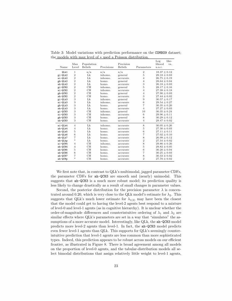
Table 3: Model variations with prediction performance on the COMBO9 dataset;the models with max level of ∗ used a Poisson distribution.
NameMaxLevel
PopulationBeliefs Precisions
PrecisionBeliefs Parameters
Log like-lihood vs.u.a.r.
QLk1 1 n/a n/a n/a 2 18.37± 0.12gi-QLk2 2 Lk inhomo. general 5 29.18± 0.03ai-QLk2 2 Lk inhomo. accurate 4 26.75± 0.19gh-QLk2 2 Lk homo. general 4 28.64± 0.04ah-QLk2 2 Lk homo. accurate 3 26.18± 0.03gi-QCH2 2 CH inhomo. general 5 28.17± 0.16ai-QCH2 2 CH inhomo. accurate 4 27.39± 0.18gh-QCH2 2 CH homo. general 4 27.90± 0.03ah-QCH2 2 CH homo. accurate 3 27.44± 0.02gi-QLk3 3 Lk inhomo. general 9 30.57± 0.17ai-QLk3 3 Lk inhomo. accurate 6 29.54± 0.27gh-QLk3 3 Lk homo. general 7 30.35± 0.20ah-QLk3 3 Lk homo. accurate 4 27.27± 0.03gi-QCH3 3 CH inhomo. general 10 30.35± 0.24ai-QCH3 3 CH inhomo. accurate 6 29.96± 0.11gh-QCH3 3 CH homo. general 8 30.29± 0.12ah-QCH3 3 CH homo. accurate 4 29.47± 0.02
ai-QLk4 4 Lk inhomo. accurate 8 30.05± 0.26ah-QLk4 4 Lk homo. accurate 5 27.30± 0.03ah-QLk5 5 Lk homo. accurate 6 27.11± 0.11ah-QLk6 6 Lk homo. accurate 7 27.02± 0.10ah-QLk7 7 Lk homo. accurate 8 26.99± 0.12ah-QLkp * Lk homo. accurate 2 27.34± 0.02ai-QCH4 4 CH inhomo. accurate 8 29.86± 0.20ah-QCH4 4 CH homo. accurate 5 29.82± 0.05ah-QCH5 5 CH homo. accurate 6 30.20± 0.04ah-QCH6 6 CH homo. accurate 7 30.25± 0.03ah-QCH7 7 CH homo. accurate 8 30.33± 0.02ah-QCHp * CH homo. accurate 2 27.70± 0.02
We first note that, in contrast to QLk’s multimodal, jagged parameter CDFs,the parameter CDFs for ah-QCH3 are smooth and (nearly) unimodal. Thissuggests that ah-QCH3 is a much more robust model; its prediction quality isless likely to change drastically as a result of small changes in parameter values.
Second, the posterior distribution for the precision parameter λ is concen-trated around 0.20, which is very close to the QLk model’s estimate for λ2. Thissuggests that QLk’s much lower estimate for λ1(2) may have been the closestthat the model could get to having the level-2 agents best respond to a mixtureof level-0 and level-1 agents (as in cognitive hierarchy). It is unclear whether theorder-of-magnitude differences and counterintuitive ordering of λ1 and λ2 aresimilar effects where QLk’s parameters are set in a way that “simulates” the as-sumptions of a more accurate model. Interestingly, like QLk, the ah-QCH3 modelpredicts more level-2 agents than level-1. In fact, the ah-QCH3 model predictseven fewer level-1 agents than QLk. This supports for QLk’s seemingly counter-intuitive prediction that level-1 agents are less common than more sophisticatedtypes. Indeed, this prediction appears to be robust across models on our efficientfrontier, as illustrated in Figure 8. There is broad agreement among all modelson the proportion of level-0 agents, and the tabular-distribution models all se-lect bimodal distributions that assign relatively little weight to level-1 agents,
23

0
0.2
0.4
0.6
0.8
1
0 0.1 0.2 0.3 0.4 0.5
Cum
ulat
ive
prob
abilit
yLevel proportions
α1α2α3
0
0.2
0.4
0.6
0.8
1
0 0.5 1 1.5 2 2.5 3 3.5 4
Cum
ulat
ive
prob
abilit
y
Precisions
λ
Figure 7: Marginal cumulative posterior distributions for the level proportionparameters (α1, α2, α3; top panel) and precision parameter (λ; bottom panel)of the ah-QCH3 model on the combined dataset.
and more to higher-level agents (level-2 and higher). The poor performance ofah-QCHp appears to follow from the fact that it models the level distribution asa (unimodal) Poisson: in order to get the “right” number of level-0 agents, themodel must place a great deal of weight on level-1 agents as well.
8.3 Spike-Poisson
If the proportion of level-0 agents were specified separately, it is possible that aPoisson distribution would better fit our data. This would have the advantageof representing higher-level agents without needing a separate parameter foreach level. In this section, we evaluate an ah-QCH model that uses just sucha distribution: a mixture of a deterministic distribution of level-0 agents, anda standard Poisson distribution. We refer to this mixture as a “spike-Poisson”distribution. Our Spike-Poisson QCH model is defined as follows:
Definition 6 (Spike-Poisson QCH model). Let πSPi,m ∈ Π(Ai) be the distributionover actions predicted for an agent i with level m by the Spike-Poisson QCHmodel. Let
f(m) =
{ε+ (1− ε)Poisson(m; τ) if m = 0,
(1− ε)Poisson(m; τ) otherwise.
Let QBRGi (s−i;λ) denote i’s quantal best response in game G to the strategy
24

0
0.2
0.4
0.6
0.8
1
0 0.1 0.2 0.3 0.4 0.5
Proportion of level-0
ah-QCHpah-QCH3ah-QCH4ah-QCH5
ah-QCH-sp
0
0.2
0.4
0.6
0.8
1
0 0.1 0.2 0.3 0.4 0.5
Proportion of level-1
0
0.2
0.4
0.6
0.8
1
0 0.1 0.2 0.3 0.4 0.5
Proportion of level-2
0
0.2
0.4
0.6
0.8
1
0 0.1 0.2 0.3 0.4 0.5
Proportion of level-3
0
0.2
0.4
0.6
0.8
1
0 0.1 0.2 0.3 0.4 0.5
Proportion of level-4
0
0.2
0.4
0.6
0.8
1
0 0.1 0.2 0.3 0.4 0.5
Proportion of level-5
Figure 8: Marginal cumulative posterior distributions of levels of reasoning forefficient frontier models.
25

1027
1028
1029
1030
1031
2 3 4 5 6
Like
lihoo
d im
prov
emen
t ove
r u.a
.r.
Number of parameters
Model performanceEfficient frontier
ah-QCHp
ah-QCH-sp
ah-QCH2
ah-QCH3
gi-QLk2 (QLk)
ah-QCH4
ah-QCH5
Figure 9: Model simplicity (number of parameters) versus prediction perfor-mance on the COMBO9 dataset, comparing the ah-QCH models of Section 8.1,QLk, and ah-QCH-sp.
profile s−i, given precision parameter λ. Let
πSPi,0:m =
m∑`=0
f(`)πSPi,`∑m`′=0 f(`′)
be the “truncated” distribution over actions predicted for an agent conditionalon that agent’s having level 0 ≤ ` ≤ m. Then πSP is defined as
πSPi,0 (ai) = |Ai|−1,πSPi,m(ai) = QBRGi (πSPi,0:m−1).
The overall predicted distribution of actions is a weighted sum of the distribu-tions for each level:
Pr(ai | τ, ε, λ) =
∞∑`=0
f(`)πSPi,` (ai).
The model thus has three parameters: the mean of the Poisson distribution τ ,the spike probability ε, and the precision λ.
Figure 9 compares the performance of ah-QCH-sp to the ah-QCH models ofSection 8.1; for reference, QLk is also included. The three-parameter ah-QCH-sp
26

model outperforms every model except for ah-QCH5. In particular, it outper-forms ah-QCH3 and ah-QCH4, despite having fewer parameters than either. Alikely explanation is that accurately modeling high-level agents (e.g., level 5)is sufficiently important that ah-QCH-sp, which includes these agents, outper-forms the models that do not; but accurately modeling the shape of the distri-bution of level-4 and level-5 agents is more important than including levels 6and up, hence ah-QCH5 outperforms ah-QCH-sp.
Overall, given the small improvement in performance between ah-QCH-spand ah-QCH5 compared to the doubling in the number of parameters required,we recommend the use of Spike-Poisson QCH for predicting human play inunrepeated normal-form games.
8.4 Generalization Performance on Unseen Games
In our cross-validated performance comparisons thus far, we have used cross-validation at the level of individual datapoints (Gi, ai). In practice, this turnsout to mean that every game in every testing fold has at least one datapoint inthe corresponding training set. That is, we never evaluate a model’s predictionson an entirely unseen game. But we claim that we can use a model fit on oneset of games to predict behavior in other, unseen games.
We checked this claim by comparing the performance of the three “efficient”models from Figure 9 using a modified cross-validation procedure. In the modi-fied procedure, we divided our combined dataset into equal-sized folds of games,with all of the datapoints for a given game being placed into a single fold. Hence,we evaluated each model entirely using games that were absent from the trainingset. We varied the number of folds from 2 (half of the games used for training,half for testing) to 128 (training on all the games but one and then testing onthe remaining game) to evaluate the importance of extra training data on gen-eralization performance. Figure 10 shows the generalization performance of theah-QCH5, ah-QCH-sp, and ah-QCHp models using this modified game-by-gamecross-validation procedure. Overall, we note that performance is very similarfor most different numbers of folds, suggesting that the models generalize wellto unseen games. The exception was the 2-fold condition, which tended to giverise to higher variance and lower performance compared to the other conditions.
9 Related work
Our work has been motivated by the question, “What model is best for predict-ing human behavior in general, simultaneous-move games?” Before beginningour study, we conducted an exhaustive literature survey to determine the extentto which this question had already been answered. Specifically, we used GoogleScholar to identify all (1698) citations to the papers introducing the QRE, CH,Lk and QLk models (McKelvey and Palfrey, 1995; Camerer et al., 2004; Nagel,1995; Stahl and Wilson, 1994), and manually checked every reference. We dis-carded superficial references, papers that simply applied one of the models to
27

1027
1028
1029
1030
1031
2 4 8 16 32 64 128
Like
lihoo
d im
prov
emen
t (re
norm
aliz
ed)
Number of folds
ah-QCH5ah-QCH-sp
ah-QCHp
Figure 10: Generalization performance of the frontier models on unseen games,with different numbers of folds, on the COMBO9 dataset. The 2-fold conditionuses half the games for training and half for test; the 4-fold condition uses 3/4 ofthe games for training and 1/4 for test; etc. Performance values are normalizedto the same scale as the 10-fold condition used elsewhere in the paper.
an application domain, and papers that studied repeated games. This left uswith a total of 21 papers (including the four with which we began), which wesummarize in Table 4. Overall, we found no paper that compared the predic-tive performance of all four models. Indeed, there were two senses in which theliterature fell short of addressing this question. First, the behavioral economicsliterature appears to be concerned more with explaining behavior than withpredicting it. Thus, comparisons of out-of-sample prediction performance wererare. Here we describe the only exceptions that we found: Morgan and Sefton(2002) and Hahn et al. (2010) evaluated prediction performance using held-outtest data; Camerer et al. (2004) and Chong et al. (2005) computed likelihoodson each individual game in their datasets after using models fit to the n− 1 re-maining games; Crawford and Iriberri (2007) compared the performance of twomodels by training each model on each game in their dataset individually, andthen evaluating the performance of each of these n trained models on each of then − 1 other individual games; and Camerer et al. (2011) evaluated the perfor-mance of QRE and cognitive hierarchy variants on one experimental treatmentusing parameters estimated on two separate experimental treatments. Second,most of the papers compared only one of the four models (often with variations)to Nash equilibrium. Indeed, only six of the 21 studies (see the bottom portionof Table 4) compared more than one of the four key models. Only three of these
28

studies explicitly compared the prediction performance of more than one of thefour models (Chong et al., 2005; Crawford and Iriberri, 2007; Camerer et al.,2011); the remaining three performed comparisons in terms of training set fit(Camerer et al., 2001; Costa-Gomes et al., 2009; Rogers et al., 2009).
Rogers et al. (2009) proposed a unifying framework that generalizes bothPoisson-CH and QRE, and compared the fit of several variations within thisframework. Notably, their framework allows for quantal response within a cog-nitive hierarchy model. Their work is thus similar to our own search over asystem of QLk variants, but there are several differences. First, we comparedout-of-sample prediction performance, not in-sample fit. Second, Rogers et al.restricted the distributions of types to be grid, uniform, or Poisson distribu-tions, whereas we considered unconstrained discrete distributions. Third, theyrequired different types to have different precisions, while we did not. Finally,we considered level-k beliefs as well as cognitive hierarchy beliefs, whereas theycompared only cognitive hierarchy belief models (although their framework inprinciple allows for both).
One line of work from the computer science literature also meets our criteriaof predicting action choices and modeling human behavior (Altman et al., 2006).This approach learns association rules between agents’ actions in different gamesto predict how an agent will play based on its actions in earlier games. We didnot consider this approach in our study, as it requires data that identifies agentsacross games, and cannot make predictions for games that are not in the trainingdataset. Nevertheless, such machine-learning-based methods could clearly beextended to apply to our setting; investigating their performance would be aworthwhile direction for future work.
10 Conclusions
To our knowledge, ours is the first study to address the question of which of theQRE, level-k, cognitive hierarchy, and quantal level-k behavioral models is bestsuited to predicting unseen human play of normal-form games. We explored theprediction performance of these models, along with several modifications. Wefound that bounded iterated reasoning and cost-proportional errors are bothcritical ingredients in a predictive model of human game theoretic behavior.The best-performing models we studied (QLk and the QCH family) combineboth of these elements.
Bayesian parameter analysis is a valuable technique for investigating thebehavior and properties of models, particularly because it is able to make quan-titative recommendations for parameter values. We showed how Bayesian pa-rameter analysis can be applied to derive concrete recommendations for theuse of an existing model, Poisson-CH, differing substantially from advice in theliterature. We also uncovered anomalies in the parameter settings of the best-performing existing model (QLk), which led us to evaluate systematic variationsof its modeling assumptions. In the end, we identified a new model family (theaccurate precision belief, homogeneous-precision QCH models) that allows the
29
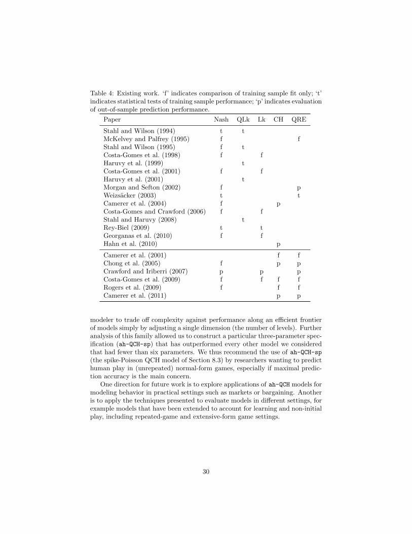
Table 4: Existing work. ‘f’ indicates comparison of training sample fit only; ‘t’indicates statistical tests of training sample performance; ‘p’ indicates evaluationof out-of-sample prediction performance.
Paper Nash QLk Lk CH QRE
Stahl and Wilson (1994) t tMcKelvey and Palfrey (1995) f fStahl and Wilson (1995) f tCosta-Gomes et al. (1998) f fHaruvy et al. (1999) tCosta-Gomes et al. (2001) f fHaruvy et al. (2001) tMorgan and Sefton (2002) f pWeizsacker (2003) t tCamerer et al. (2004) f pCosta-Gomes and Crawford (2006) f fStahl and Haruvy (2008) tRey-Biel (2009) t tGeorganas et al. (2010) f fHahn et al. (2010) p
Camerer et al. (2001) f fChong et al. (2005) f p pCrawford and Iriberri (2007) p p pCosta-Gomes et al. (2009) f f f fRogers et al. (2009) f f fCamerer et al. (2011) p p
modeler to trade off complexity against performance along an efficient frontierof models simply by adjusting a single dimension (the number of levels). Furtheranalysis of this family allowed us to construct a particular three-parameter spec-ification (ah-QCH-sp) that has outperformed every other model we consideredthat had fewer than six parameters. We thus recommend the use of ah-QCH-sp(the spike-Poisson QCH model of Section 8.3) by researchers wanting to predicthuman play in (unrepeated) normal-form games, especially if maximal predic-tion accuracy is the main concern.
One direction for future work is to explore applications of ah-QCH models formodeling behavior in practical settings such as markets or bargaining. Anotheris to apply the techniques presented to evaluate models in different settings, forexample models that have been extended to account for learning and non-initialplay, including repeated-game and extensive-form game settings.
30

References
Altman, A., Bercovici-Boden, A., and Tennenholtz, M. (2006). Learning inone-shot strategic form games. In ECML, pages 6–17.
Arad, A. and Rubinstein, A. (2011). The 11-20 money request game: A level-kreasoning study. http://www.tau.ac.il/~aradayal/moneyrequest.pdf.
Becker, T., Carter, M., and Naeve, J. (2005). Experts playing the traveler’sdilemma. Diskussionspapiere aus dem Institut fr Volkswirtschaftslehre derUniversitt Hohenheim 252/2005, Department of Economics, University of Ho-henheim, Germany.
Bishop, C. (2006). Pattern recognition and machine learning. Springer.
Camerer, C., Ho, T., and Chong, J. (2001). Behavioral game theory: Thinking,learning, and teaching. Nobel Symposium on Behavioral and ExperimentalEconomics.
Camerer, C., Ho, T., and Chong, J. (2004). A cognitive hierarchy model ofgames. QJE, 119(3):861–898.
Camerer, C., Nunnari, S., and Palfrey, T. R. (2011). Quantal response andnonequilibrium beliefs explain overbidding in maximum-value auctions. Work-ing paper, California Institute of Technology.
Camerer, C. F. (2003). Behavioral Game Theory: Experiments in StrategicInteraction. Princeton University Press.
Chong, J., Camerer, C., and Ho, T. (2005). Cognitive hierarchy: A limitedthinking theory in games. Experimental Business Research, Vol. III: Market-ing, accounting and cognitive perspectives, pages 203–228.
Cooper, D. and Van Huyck, J. (2003). Evidence on the equivalence of thestrategic and extensive form representation of games. JET, 110(2):290–308.
Costa-Gomes, M. and Crawford, V. (2006). Cognition and behavior in two-person guessing games: An experimental study. AER, 96(5):1737–1768.
Costa-Gomes, M., Crawford, V., and Broseta, B. (1998). Cognition and behaviorin normal-form games: an experimental study. Discussion paper 98-22, UCSD.
Costa-Gomes, M., Crawford, V., and Broseta, B. (2001). Cognition and behaviorin normal-form games: An experimental study. Econometrica, 69(5):1193–1235.
Costa-Gomes, M., Crawford, V., and Iriberri, N. (2009). Comparing modelsof strategic thinking in Van Huyck, Battalio, and Beil’s coordination games.JEEA, 7(2-3):365–376.
31
Crawford, V. and Iriberri, N. (2007). Fatal attraction: Salience, naivete, andsophistication in experimental “hide-and-seek” games. AER, 97(5):1731–1750.
Gao, X. A. and Pfeffer, A. (2010). Learning game representations from datausing rationality constraints. In UAI-10, pages 185–192.
Georganas, S., Healy, P. J., and Weber, R. (2010). On the persistence of strategicsophistication. Working paper, University of Bonn.
Gill, J. (2002). Bayesian methods: A social and behavioral sciences approach.CRC press.
Goeree, J. K. and Holt, C. A. (2001). Ten little treasures of game theory andten intuitive contradictions. AER, 91(5):1402–1422.
Hahn, P. R., Lum, K., and Mela, C. (2010). A semiparametric model for as-sessing cognitive hierarchy theories of beauty contest games. Working paper,Duke University.
Haruvy, E. and Stahl, D. (2007). Equilibrium selection and bounded rationalityin symmetric normal-form games. JEBO, 62(1):98–119.
Haruvy, E., Stahl, D., and Wilson, P. (1999). Evidence for optimistic andpessimistic behavior in normal-form games. Economics Letters, 63(3):255–259.
Haruvy, E., Stahl, D., and Wilson, P. (2001). Modeling and testing for hetero-geneity in observed strategic behavior. Review of Economics and Statistics,83(1):146–157.
Ho, T., Camerer, C., and Weigelt, K. (1998). Iterated dominance and iteratedbest response in experimental” p-beauty contests”. The American EconomicReview, 88(4):947–969.
McKelvey, R., McLennan, A., and Turocy, T. (2007). Gambit: Software toolsfor game theory, version 0.2007. 01.30.
McKelvey, R. and Palfrey, T. (1995). Quantal response equilibria for normalform games. GEB, 10(1):6–38.
Morgan, J. and Sefton, M. (2002). An experimental investigation of unprofitablegames. GEB, 40(1):123–146.
Nagel, R. (1995). Unraveling in guessing games: An experimental study. AER,85(5):1313–1326.
Neal, R. M. (2001). Annealed importance sampling. Statistics and Computing,11(2):125–139.
Nelder, J. A. and Mead, R. (1965). A simplex method for function minimization.Computer Journal, 7(4):308–313.
32

Rey-Biel, P. (2009). Equilibrium play and best response to (stated) beliefs innormal form games. GEB, 65(2):572–585.
Robert, C. P. and Casella, G. (2004). Monte Carlo statistical methods. SpringerVerlag.
Rogers, B. W., Palfrey, T. R., and Camerer, C. F. (2009). Heterogeneous quantalresponse equilibrium and cognitive hierarchies. JET, 144(4):1440–1467.
Stahl, D. and Haruvy, E. (2008). Level-n bounded rationality and dominatedstrategies in normal-form games. JEBO, 66(2):226–232.
Stahl, D. and Wilson, P. (1994). Experimental evidence on players’ models ofother players. JEBO, 25(3):309–327.
Stahl, D. and Wilson, P. (1995). On players’ models of other players: Theoryand experimental evidence. GEB, 10(1):218–254.
Turocy, T. (2005). A dynamic homotopy interpretation of the logistic quan-tal response equilibrium correspondence. Games and Economic Behavior,51(2):243–263.
Von Neumann, J. and Morgenstern, O. (1944). Theory of Games and EconomicBehavior. Princeton University Press.
Weizsacker, G. (2003). Ignoring the rationality of others: evidence from exper-imental normal-form games. GEB, 44(1):145–171.
Witten, I. H. and Frank, E. (2000). Data Mining: Practical Machine LearningTools and Techniques with Java Implementations. Morgan Kaufmann.
33