Embed Size (px)
Citation preview

IT 13 006
Examensarbete 30 hpJanuari 2013
Evaluating NOSQL Technologies for Historical Financial Data
Ansar Rafique
Institutionen för informationsteknologiDepartment of Information Technology


Teknisk- naturvetenskaplig fakultet UTH-enheten Besöksadress: Ångströmlaboratoriet Lägerhyddsvägen 1 Hus 4, Plan 0 Postadress: Box 536 751 21 Uppsala Telefon: 018 – 471 30 03 Telefax: 018 – 471 30 00 Hemsida: http://www.teknat.uu.se/student
Abstract
Evaluating NOSQL Technologies for HistoricalFinancial Data
Ansar Rafique
Today, when businesses and organizations are generating huge volumes of data; theapplications like Web 2.0 or social networking requires processing of petabytes ofdata. Stock Exchange Systems are among the ones that process large amount ofquotes and trades on a daily basis. The limited database storage ability is a majorbottleneck in meeting up the challenge of providing efficient access to information.
Further to this, varying data are the major source of information for the financialindustry. This data needs to be read and written efficiently in the database; this isquite costly when it comes to traditional Relational Database Management System.RDBMS is good for different scenarios and can handle certain types of data very well,but it isn’t always the perfect choice. The existence of innovative architectures allowsthe storage of large data in an efficient manner.
“Not only SQL” brings an effective solution through the provision of an efficientinformation storage capability. NOSQL is an umbrella term for various new datastore. The NOSQL databases have gained popularity due to different factors thatinclude their open source nature, existence of non-relational data store,high-performance, fault-tolerance, and scalability to name a few. Nowadays, NOSQLdatabases are rapidly gaining popularity because of the advantages that they offercompared to RDBMS.
The major aim of this research is to find an efficient solution for storing andprocessing the huge volume of data for certain variants. The study is based onchoosing a reliable, distributed, and efficient NOSQL database at Cinnober FinancialTechnology AB. The research majorly explores NOSQL databases and discussesissues with RDBMS; eventually selecting a database, which is best suited for financialdata management. It is an attempt to contribute the current research in the field ofNOSQL databases which compares one such NOSQL database Apache Cassandrawith Apache Lucene and the traditional relational database MySQL for financialmanagement.
The main focus is to find out which database is the preferred choice for differentvariants. In this regard, the performance test framework for a selected set ofcandidates has also been taken into consideration.
Keywords: NOSQL, Apache Cassandra, MySQL, Financial data, Historical data,Benchmark performance.
Tryckt av: Reprocentralen ITCIT 13 006Examinator: Lisa KaatiÄmnesgranskare: Erik ZeitlerHandledare: Lars Albertsson


1 | P a g e
Acknowledgements
My foremost thanks and praise goes to Almighty ALLAH, without whose compassion and
mercifulness I wouldn’t have been able to finalize my Master’s project and thesis.
I offer profound gratitude to Cinnober Financial Technology AB Company for introducing
me to the problem and offering me the resources to perform the research work and
implementation. I am greatly obliged to Cinnober Financial Technology AB for bringing in
such a great opportunity to me. I was offered a warm working atmosphere during my stay
at Cinnober Financial Technology AB, and I am really grateful to all the people who were
directly or indirectly involved in my project. I particularly acknowledge the help of Nick
Bailey, Asma Khurshid, Shehla Rafique Khan, Olle Eriksson, Samiaa Munawar, and Sameen
Shaukat.
Moreover, I would like to gratefully thank Lars Albertsson for his supervision, guidance, and
support throughout the thesis work. His cooperation and supervision has been a major
source of motivation for me that helped me to successfully attain my goal. I would also like
to offer my gratitude to Erik Zeitler for his kind support, especially in the report write-up.
Finally, credit goes to my family and friends for their prayers and support that they
extended towards me throughout the project.

2 | P a g e
Abbreviations
HS History Server QS Query Server ACID Atomicity, Consistency, Isolation, and Durability CAP Consistency, Availability, and Partition Tolerance DB Database DBs Databases DBAs Database Administrators RDBMS Relational Database Management System SQL Structured Query Language NOSQL Not Only SQL AP Availability and Partition Tolerance CP Consistency and Partition Tolerane CA Consistency and Availability K-V Key-Value CF Column Family RP Random Partitioner OPP Order Preserving Partitioner SSTable Sorted String Table I/O Input/Output CPUs Central Processing Units CLI Command Line Interface MD5 Message Digest Algorithm J2SE Java to Standard Edition Java EE Java Enterprise Edition J2EE Java to Enterprise Edition Java ME Java Micro Edition J2ME Java to Mobile Edition JBC Java Byte Code JVM Java Virtual Machine VMs Virtual Machines JDBC Java Database Connectivity JNDI Java Naming Directory Interface RMI Remote Method Invocation AWT Abstract Window Toolkit JSP Java Server Pages JSF Java Server Faces EJB Enterprise Java Beans APIs Application Programming Interface CQL Cassandra Query Language HDFS Hadoop Distributed File System IDE Integrated Development Environment HTML HyperText Markup Language MVCC Multiversion Concurrency Control RPC Remote Procedure Calls

3 | P a g e
Contents
Acknowledgements ................................................................................................................................. 1
Abbreviations .......................................................................................................................................... 2
1. Introduction ................................................................................................................................... 11
1.1. The Organization ................................................................................................................... 11
1.2. Research Background ............................................................................................................ 11
1.3. Tasks ...................................................................................................................................... 12
1.4. Thesis Outline ........................................................................................................................ 12
2. Related Work ................................................................................................................................. 13
3. Theoretical Basics .......................................................................................................................... 14
3.1. Relational Database Management System (RDBMS) ............................................................ 14
3.1.1. Table .............................................................................................................................. 14
3.1.2. Record/Field .................................................................................................................. 14
3.1.3. Column .......................................................................................................................... 15
3.1.4. SQL Constraints ............................................................................................................. 15
3.1.5. Data Integrity ................................................................................................................. 15
3.2. ACID MODEL .......................................................................................................................... 15
3.2.1. Atomicity ....................................................................................................................... 16
3.2.2. Consistency .................................................................................................................... 16
3.2.3. Isolation ......................................................................................................................... 16
3.2.4. Durability ....................................................................................................................... 16
3.3. Scalability in RDBMS .............................................................................................................. 16
3.3.1. Sharding ......................................................................................................................... 16
3.3.2. Replication ..................................................................................................................... 17
3.4. Apache Lucene ...................................................................................................................... 18
3.5. Not Only SQL (NOSQL) ........................................................................................................... 18
3.5.1. NOSQL Categories ......................................................................................................... 18
3.5.1.1. Key-Value Store ..................................................................................................... 19
Example ..................................................................................................................................... 19
3.5.1.2. Column Family/BigTable Clone.............................................................................. 19
Example ..................................................................................................................................... 19
3.5.1.3. Document Databases ............................................................................................ 20
Example ..................................................................................................................................... 20
4 | P a g e
3.5.1.4. Graph Databases ................................................................................................... 20
Example ..................................................................................................................................... 20
3.5.2. NOSQL Data Model ........................................................................................................ 21
3.6. CAP Theorem ......................................................................................................................... 21
3.6.1. Consistency .................................................................................................................... 21
3.6.2. Availability ..................................................................................................................... 21
3.6.3. Partition Tolerance ........................................................................................................ 21
3.6.4. Choose any two ............................................................................................................. 21
3.7. Difference between RDBMS and NOSQL............................................................................... 22
3.7.1. When to choose RDBMS................................................................................................ 22
3.7.2. NOSQL and RDBMS Data Store...................................................................................... 23
3.7.3. When to choose NOSQL ................................................................................................ 24
3.7.4. Why RDBMS does not scale and NOSQL does? ............................................................. 24
4. Analysis .......................................................................................................................................... 25
4.1. Distributed Database ............................................................................................................. 25
4.1.1. Advantages of Distributed Databases ........................................................................... 25
4.1.1.1. Data Replication .................................................................................................... 26
4.1.1.2. Horizontally Fragmented data ............................................................................... 26
4.1.1.3. Vertically Fragmented data ................................................................................... 26
4.1.1.4. Improved Performance ......................................................................................... 26
4.2. Popular NOSQL Databases Comparison ................................................................................ 26
4.2.1. MONGODB..................................................................................................................... 26
4.2.2. CouchDB ........................................................................................................................ 27
4.2.3. Hadoop/HBase (V0.92.0) ............................................................................................... 27
4.2.4. Apache Cassandra ......................................................................................................... 28
4.2.5. RIAK (V1.0) ..................................................................................................................... 28
4.2.6. Redis (V2.4) .................................................................................................................... 29
4.2.7. Membase ....................................................................................................................... 29
4.3. What’s wrong with Relational Database Management Systems (RDBMS)? ......................... 29
4.4. What’s wrong with Lucene? .................................................................................................. 31
4.5. NOSQL Category Selection and Motivation .......................................................................... 31
4.6. NOSQL Database Selection .................................................................................................... 32
4.6.1. Difference between HBase and Cassandra ................................................................... 32
4.6.1.1. Apache Hadoop/HBase .......................................................................................... 32
5 | P a g e
4.6.1.2. Apache Cassandra ................................................................................................. 32
4.6.2. Motivation for Selected Database ................................................................................. 33
5. Apache Cassandra – Distributed Database ................................................................................... 34
5.1. Cassandra Data Store ............................................................................................................ 34
5.2. Cassandra Architecture ......................................................................................................... 35
5.2.1. Internodes Communication ........................................................................................... 35
5.2.2. Cluster Membership and Seed Node ............................................................................ 36
5.2.3. Failure Detection and Recovery .................................................................................... 36
5.3. Data Partitioning in Cassandra .............................................................................................. 36
5.4. Partitioning Types .................................................................................................................. 37
5.4.1. Random Partitioner ....................................................................................................... 37
5.4.2. Order Preserving Partitioners ........................................................................................ 37
5.5. Replication in Cassandra ....................................................................................................... 37
5.6. Replica Placement Strategy ................................................................................................... 37
5.6.1. Simple Strategy .............................................................................................................. 37
5.6.2. NetworkTopologyStrategy ............................................................................................ 38
5.7. Client Requests in Cassandra ................................................................................................ 39
5.7.1. Write Request ................................................................................................................ 39
5.7.2. Read Request ................................................................................................................. 40
5.8. Indexes in Cassandra ............................................................................................................. 41
5.8.1. Primary Index ................................................................................................................ 41
5.8.2. Alternate Index .............................................................................................................. 41
5.8.3. Native Secondary Indexes (Built-in) .............................................................................. 41
5.8.4. Build Custom Secondary Index ...................................................................................... 42
5.8.5. Use Secondary Index ..................................................................................................... 42
5.8.5.1. Create New Column Family with Index ................................................................. 42
5.8.5.2. Create Index on existing column family ................................................................ 42
5.9. How Cassandra differs from RDBMS ..................................................................................... 42
5.10. Tuning Cassandra for Improving Performance .................................................................. 43
5.10.1. Improve writes performance ........................................................................................ 43
5.10.2. Improve read performance ........................................................................................... 43
5.11. Node Configuration Option ............................................................................................... 44
5.12. Gossip Settings .................................................................................................................. 44
5.13. High level clients in Cassandra .......................................................................................... 44
6 | P a g e
6. Implementation Environment ....................................................................................................... 47
6.1. Java ........................................................................................................................................ 47
6.1.1. Java to Standard Edition (J2SE) ..................................................................................... 47
6.1.2. Java Enterprise Edition (Java EE) ................................................................................... 47
6.1.3. Java Micro Edition (Java ME) ......................................................................................... 47
6.2. Apache Lucene ...................................................................................................................... 48
6.3. Java Database Connectivity (JDBC) ....................................................................................... 48
MYSQLJDBCConnector .................................................................................................................. 49
6.4. Cassandra Query Language - JDBC (CQL-JDBC) ..................................................................... 50
CQLJDBCConnector ....................................................................................................................... 50
6.5. JUNIT...................................................................................................................................... 52
6.6. JFreeChart .............................................................................................................................. 52
6.7. MySQL ................................................................................................................................... 52
6.8. Apache Cassandra ................................................................................................................. 52
7. Testing and Evaluation .................................................................................................................. 53
7.1. Benchmark Configuration ..................................................................................................... 54
7.1.1.1. MySQL Write ......................................................................................................... 54
7.1.1.2. MySQL find by primary key ................................................................................... 55
7.1.1.3. MySQL find by parameters .................................................................................... 56
7.1.2. Apache Cassandra ......................................................................................................... 57
7.1.2.1. Cassandra Write .................................................................................................... 57
7.1.2.2. Cassandra find by key ............................................................................................ 58
7.1.2.3. Cassandra find by parameters ............................................................................... 59
7.1.3. Apache Lucene .............................................................................................................. 60
7.1.3.1. Lucene Write ......................................................................................................... 60
7.1.3.2. Lucene find by parameters .................................................................................... 61
7.2. Performance Analysis ............................................................................................................ 62
7.2.1. Write Performance ........................................................................................................ 62
7.2.2. Read Performance ......................................................................................................... 63
7.2.2.1. Find by Key ................................................................................................................ 63
7.2.2.2. Find by Parameter ..................................................................................................... 63
7.2.3. Reason for MySQL slow write........................................................................................ 63
7.2.4. Reason for Cassandra slow read ................................................................................... 64
8. Conclusion ..................................................................................................................................... 65

7 | P a g e
8.1. Future work ........................................................................................................................... 66
8 | P a g e
List of Figures
Figure 1- Example of Sharding Technique .......................................................... 17
Figure 2- Master Slave architecture ................................................................. 17
Figure 3-Indexing Lucene Architecture ............................................................. 18
Figure 4- Key-Value Store ............................................................................ 19
Figure 5- Graph Database ............................................................................ 20
Figure 6- NOSQL Data Model ......................................................................... 21
Figure 7- RDBMS and NOSQL data store and process ............................................. 23
Figure 8- Distributed Databases ..................................................................... 25
Figure 9- Where RDBMS Stand ....................................................................... 30
Figure 10- Cassandra Data Store Architecture ..................................................... 34
Figure 11- Cassandra Data Partition ................................................................ 36
Figure 12- Cassandra Simple Strategy Replication ................................................ 38
Figure 13- Cassandra Network Topology Strategy Replication .................................. 39
Figure 14- Cassandra Write Request ................................................................ 40
Figure 15- Cassandra Read Request ................................................................. 41
Figure 16- Application Interface ..................................................................... 48
Figure 17- JDBC Connectivity ........................................................................ 49
Figure 18- MySQL Write Performance ............................................................... 54
Figure 19- MySQL Write Performance ............................................................... 55
Figure 20- MySQL Find by Key Performance ....................................................... 55
Figure 21- MySQL Find by Key Performance ....................................................... 56
Figure 22- MySQL Find by Parameter Performance ............................................... 56
Figure 23- MySQL Find by Parameter Performance ............................................... 57
Figure 24- Cassandra Write Performance .......................................................... 57
Figure 25- Cassandra Write Performance .......................................................... 58
Figure 26- Cassandra Find by Key Performance ................................................... 58
9 | P a g e
Figure 27- Cassandra Find by Key Performance ................................................... 59
Figure 28- Cassandra Find by Parameter Performance ........................................... 59
Figure 29- Cassandra Find by Parameter Performance ........................................... 60
Figure 30- Lucene Write Performance .............................................................. 60
Figure 31- Lucene Write Performance .............................................................. 61
Figure 32- Lucene Find by Parameter Performance .............................................. 61
Figure 33- Lucene Find by Parameter Performance .............................................. 62
10 | P a g e
List of Tables
Table 1- Table in RDBMS .............................................................................. 14
Table 2- Record/Field in RDBMS ..................................................................... 14
Table 3- Column in RDBMS ........................................................................... 15
11 | P a g e
Chapter 1
1. Introduction
This chapter aims to provide an introduction of the research work and project that was
conducted to complete this thesis. Initially, an overview of the organizational history has
been presented for Cinnober Financial Technology AB followed by the research
background, tasks, and thesis outline.
1.1. The Organization Cinnober Financial Technology AB was founded in 1998 in Stockholm, Sweden. The
Company provides solutions for exigent trading and clearing venues by supplying advanced
technology systems for financial market. Cinnober Financial Technology AB powers some of
the most demanding financial marketplaces in the world for example, Alpha Exchange,
American Stock Exchange, etc. The organization specializes in managing and supporting
mission-critical marketplace solutions. The major products offered by Cinnober Financial
technology AB are based on TRADExpress. TRADExpress is a Java-based platform that offers
fully redundant and scalable architecture [19].
1.2. Research Background There are different types of databases and architectures that have been designed to
process data from varied sources of information. Previously, the relational model was the
dominant choice among all database models, and nearly all databases followed the same
basic architecture. However, the recent innovations in the field of technology have made
the developers realize that the relational model is not always the best choice. This motive
has resulted in the development of other architectures that offer more scalability and
flexibility for storing information in a reliable manner. For Example; today the major
internet companies such as Google, Amazon, and Facebook are not only using relational
model, but have also developed their own architecture to store large amount of data in
the database in a more efficient manner. The intent behind this thesis is to find an
efficient solution for storing and processing huge amounts of data at Cinnober Financial
Technology AB.
Traditional Relational Database Management Systems (RDBMS) are hard to scale large
chunks of information or data. Stock Exchange Trading System provides access to financial
market data, e.g. stock quotes and volumes. The system is required to process huge
volume of quotes and trades each day. Summing up the historical market information,
results in the generation of significant data. Traditional RDBMS brings a bottleneck in this
scenario because it does not have the ability to meet the challenge of providing efficient
access to this information.
This research mainly focuses on how to improve the History Server (HS). HS uses Hibernate
framework for the persistence of data and MySQL database for the permanent back-end
storage. HS contains 30 days data and for the financial industry it can be a huge amount of
data. Along with HS there is another server called Query Server (QS). QS contains up-to-

12 | P a g e
date information and store only one day data. RDBMS is not always the perfect choice for
storing and processing the large volume of data mainly when the concern is only reading
and writing, delete and update operations are not involved nor consistency required.
Consistency is not an issue in case of HS because if the up-to-date information is required
then it is also available in QS. The purpose of research work and the experiments described
in Testing and Evaluation is to find the other architectures which can replace MySQL and
get the understanding of how different architectures behave for different variants.
1.3. Tasks The main task of this thesis is to research Not Only SQL (NOSQL) databases. The research
mainly covers topics like; what makes NOSQL better than Relational Database Management
Systems (RDBMS), when to use RDBMS and when to use NOSQL, and how to make NOSQL
category and database selection. Furthermore, the research work evaluates NOSQL
database by testing its suitability for the Financial Industry. In this regard, a performance
test framework has been built for selected set of candidate technologies and traditional
SQL databases as a reference.
1.4. Thesis Outline The first section of the report explains the Scalability limitations in Relational Database
Management Systems (RDBMS) and provides an overview of Not Only SQL (NOSQL)
databases. Advantages of NOSQL databases and how these solve the limitations that are
typically found in case of using RDBMS is discussed. Furthermore, comparison of few NOSQL
databases is presented.
The second section explains, Apache Cassandra and its architecture in detail, and further
evaluates how different databases behave for different variants in terms of read and write
throughput. The evaluation is done by creating a performance benchmark for Apache
Cassandra, while keeping RDBMS and Apache Lucene as reference.
The following is an outline of the thesis structure:
Chapter 2: Explains concepts of Relational Database Management Systems (RDBMS),
Atomicity, Consistency, Isolation, and Durability (ACID) Model, Salability in RDBMS, Apache
Lucene, Not Only SQL (NOSQL), Consistency, Availability, and Partition Tolerance (CAP)
Theorem, discusses the difference between RDBMS and NOSQL, and why RDBMS do not
scale and NOSQL does.
Chapter 3: Explains distributed databases, popular Not Only SQL (NOSQL) databases,
limitations with Relational Database Management Systems (RDBMS), NOSQL category
selection, NOSQL database selection, and difference between Cassandra and HBase.
Chapter 4: Gives a brief introduction about Apache Cassandra and its architecture.
Chapter 5: Describes the tools and technologies used for the implementation work.
Chapter 6: Explains test and performance evaluations of Apache Lucene, Relational
Database Management Systems (RDBMS), and Apache Cassandra.
Chapter 7: Concludes the work.
13 | P a g e
Chapter 2
2. Related Work
The thesis evaluates Not Only SQL (NOSQL) technologies in general, compares different
NOSQL databases, discusses the limitations with Relational Database Management Systems
(RDBMS), and gives an understanding of how different databases behave for different
variants with different amounts of data in the database. Below is the list of related work
and how these differ from the work in this thesis.
The thesis “No Relation: The Mixed Blessings of Non Relational Databases” [31]
gives a good understanding of non-relational data stores. The author discusses the
non-relational data stores in detail and how they differ from relational data stores.
Comparison of both data models in terms of strengths and weaknesses has also been
discussed. Non-relational data stores gained popularity when developers started to
realize that there was a need to find an alternative, then non relational data store
and new efficient architectures were developed to make the data read and write
fast such as in memory data store and process. As the thesis is more than three
years old, some parts are already outdated as new architectures have been
developed or modified for good read and write performance. For example, the
author discusses super columns in Cassandra which are not recommended to use
anymore.
The thesis “Cassandra” [25] gives a good understanding of Apache Cassandra. The
author identifies the limitations that exist in RDBMS and how these limitations can
be solved using Apache Cassandra such as Scalability. Moreover, differences
between Cassandra and RDBMS have also been discussed from different point of
views. As thesis is more than two years old, new concepts are not discussed such as
Cassandra data store, Cassandra architecture, Cassandra replication strategy,
Cassandra data partition, how Cassandra handles read and write requests, and
different indexes techniques in Cassandra for efficient data access. Cassandra is an
open source project which makes it strong candidate to progress in the next few
years. Many wrappers over Remote Procedure Calls (RPC) client have developed for
different programming languages described in High level clients in Cassandra
which are also not discussed.
There is no doubt that NOSQL databases are getting popularity, but according to
Database Administrators (DBAs) NOSQL has an immature data store. NOSQL
proponents react with the argument that RDBMS does not scale large data volume
well. The author has not found any example where NOSQL has been used to store
financial data. Kristof Kovacs blog NOSQL Database Comparison [4] compares
different popular NOSQL databases and identifies the situation in which they are
best to use. According to author, Apache Cassandra is mostly suited for banking and
financial industry [4].
14 | P a g e
Chapter 3
3. Theoretical Basics
In order to fully understand this report, reader should be familiar with the topics in this
chapter.
3.1. Relational Database Management System (RDBMS) Relational Database Management Systems (RDBMS) is based on relational model which was
introduced by E. F. Codd. RDBMS is the basis for Structured Query Language (SQL) and
modern database systems like Oracle, MS SQL Server, MySQL, and PostgreSQL [8].
In general, RDBMS provides following features:
Data are stored in tables.
Data storage is in the form of rows and columns.
Primary keys are used to uniquely classify the rows.
Indexing facility makes the data retrieval faster.
Databases allow the creation of views or virtual tables.
Primary and foreign keys can be used to define relationship between two entities,
i.e. the existence of a common column between two tables.
Multi-user accessibility
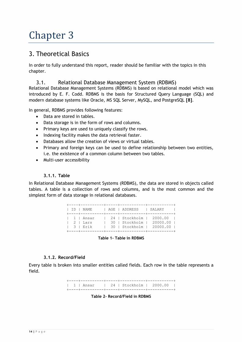
3.1.1. Table
In Relational Database Management Systems (RDBMS), the data are stored in objects called
tables. A table is a collection of rows and columns, and is the most common and the
simplest form of data storage in relational databases.
+----+----------+-----+-----------+-----------+
| ID | NAME | AGE | ADDRESS | SALARY |
+----+----------+-----+-----------+-----------+
| 1 | Ansar | 24 | Stockholm | 2000.00 |
| 2 | Lars | 30 | Stockholm | 20000.00 |
| 3 | Erik | 30 | Stockholm | 20000.00 |
+----+----------+-----+-----------+-----------+
Table 1- Table in RDBMS
3.1.2. Record/Field
Every table is broken into smaller entities called fields. Each row in the table represents a
field.
+----+----------+-----+-----------+-----------+
| 1 | Ansar | 24 | Stockholm | 2000.00 |
+----+----------+-----+-----------+-----------+
Table 2- Record/Field in RDBMS

15 | P a g e
3.1.3. Column
Every record is divided into smaller attributes called columns. A Column is a vertical entity
in a table that contains all the information associated with a specific record in a table.
+-----------+
| ADDRESS |
+-----------+
| Stockholm |
| Stockholm |
| Stockholm |
+-----------+
Table 3- Column in RDBMS
3.1.4. SQL Constraints
Constraints are the rules enforced on data columns in the table. Constraints ensure the
reliability and accuracy of data in the database [8].
Following are the common constraints available in SQL:
Not NULL Constraint: It ensures that the column cannot have NULL value.
DEFAULT Constraint: Provides default value for a column when nothing is specified for a column value.
UNIQUE Constraint: Ensures that all values in a column are different, i.e. Values of two columns are not same.
PRIMARY Key: Uniquely identifies each record in a table.
FOREIGN Key: Uniquely identify records in the referenced table.
CHECK Constraint: Ensures that all values in a column satisfy certain conditions.
INDEX: Used to retrieve the data from the database very quickly.
3.1.5. Data Integrity
The following data integrity constraints exist with each RDBMS.
Entity Integrity: It ensures that there are no duplicate rows in the table.
Referential integrity: It states that each foreign key value in a relation must have a
corresponding primary key value in base table.
Domain Integrity: It ensures the validity of the values for the column by restricting
type, format, and range of values.
User-defined Integrity: It allows the enforcement of some specific business rules
from the user.
3.2. ACID MODEL According to Mike Chapple [3] Atomicity, Consistency, Isolation, and Durability (ACID)
model is one of the oldest and important concepts of database. It sets following four goals
that must be achieved by database for ensuring reliability:
16 | P a g e
3.2.1. Atomicity
Atomicity states that each transaction should be “italics” which means that transaction
should be either completely executed or executed not at all. If one part of the transaction
fails then entire transaction should fail [3].
3.2.2. Consistency
Consistency states that only valid data should be written to the database. If a transaction
is executed that violates the database consistency rules, then the entire transaction will
be rolled back [3]. If a transaction executes successfully, then it should take the database
from one consistent state to another.
3.2.3. Isolation
Isolation states that the transactions should be executed independent of each other. For
example, if Ansar issues a transaction on database ‘A’ and Lars issues another transaction
on the same database at the same time, then both transactions should operate on the
database in an isolated manner. The database should perform Ansar’s transaction before
executing Lars’s transaction or vice versa. This will prevent Lars’s transaction from reading
intermediate data that were produced by Ansar’s transaction, which is still yet to be
committed in the database.
3.2.4. Durability
Durability ensures that transaction that has been committed to the database will not be
lost. Durability is ensured through the employment of database backups and transaction
logs.
Looking at the Atomicity, Consistency, Isolation, and Durability (ACID) properties in detail,
it is certain that read operations alone do not violate any ACID properties. It is only
possible to violate when the write operations are involved.
3.3. Scalability in RDBMS Scalability is required in order to handle more requests. It is achieved either by upgrading
the hardware of existing nodes or by adding more nodes. Scalability became one of the
most important and desired properties of any database [25] because of exponential growth
of data. Due to exponential growth of data it is not possible for a single server to store
huge amount of data and process thousands of user requests. To cope with such scenario,
scalability is required. Sharding and Replication are two common techniques that improve
Scalability [25].
3.3.1. Sharding
In a Sharding databases, data are portioned across different nodes. The easiest technique
is to move heavily used table to another node and let the node to handle table requests for
both read and write. This technique can helps to achieve data sharding, but it is not
possible to move the table to another node because what will happen if the table has
outgrown a new node? The other technique is to manually assign ranges to each node and
split the rows across the node where each node is responsible for specific row ranges, let
the look-up service to decide which node holds which rows. [25].

17 | P a g e
Sharding is definitely a solution to handle scalability, but with some limitations. With
manually assigned ranges to each server there is a big risk of overloading a single node for
both reads and writes operations; also it is not always possible to achieve the Sharding
because of table based nature of Relational Database Management Systems (RDBMS).
Sharding requires the distinct entities to store across the nodes [25].
Figure 1- Example of Sharding Technique
3.3.2. Replication
Replication is a technique to improve the number of reads and writes operations. The
simple strategy is to create master and slave architecture. Writes are sent to master and
pushed to slaves while reads are sent to slave to handle directly [25].
The limitation with this approach is, if the master node goes down, then writes operations
cannot be performed.
Figure 2- Master Slave architecture

18 | P a g e
3.4. Apache Lucene Apache Lucene is a high performance, open source, text search engine library that is
entirely written in Java. It allows the searching and indexing functionality to the
applications [5].
Lucene stores different types of documents and for each document there is a separate
parser that does some pre-processing. For example, HyperText Markup Language (HTML)
parser filters the HTML tag and outputs the text content. Lucene Analyzer extracts tokens
and related information such as token frequency and writes the tokens and related
information to the index file of Lucene [6].
Figure 3-Indexing Lucene Architecture
3.5. Not Only SQL (NOSQL) Non-Relational data that does not need to be fixed schema for storage, usually avoids join
operations, and typically scales horizontally [32]. Not only SQL (NOSQL) databases trade-
off Atomicity, Consistency, Isolation, and Durability (ACID) properties by introducing
following features:
NOSQL is not “NEVER SQL”
NOSQL is not “NO SQL”
NOSQL is “NOT ONLY SQL”
Rather, NOSQL means that back-end features will consist of not only Structured Query
Language (SQL) databases, but also key value store, column family/big table clone, graph
databases, and document databases.
3.5.1. NOSQL Categories
Key-Value Store
Column Family/BigTable Clone
Document Databases
Graph Databases

19 | P a g e
3.5.1.1. Key-Value Store
A research paper published by Amazon [28] states that Amazon achieves scalability
not only by Structured Query Language (SQL), but to meet reliability and scalability
Amazon has developed a number of storage technologies, the simplest one is called
Dynamo, which is based on key-value store. A Key-value store uses a hash table
where there is a unique key and pointer to particular data items [29].
Data Model: Collection of Key-Value Pairs.
In key-value stores, values are indexed and retrieved by keys [27].
Key-Value model is the simplest and easiest to implement because it is popular in
different programming languages.
Among other disadvantages, it is inefficient when the interest is only on querying or
updating the specific part of the value rather than the whole value.
Example
RIAK
Voldemort used at Linkedin
Tokyo
Figure 4- Key-Value Store
3.5.1.2. Column Family/BigTable Clone
Column Family/BigTable is based on Google BigTable Paper [30]. Like Amazon
Google also scale systems by using not only Structured Query Language (SQL)
databases, but also using alternative implementation called BigTable.
Data Models: BigTable, Column Family.
The unique thing about Column Family/BigTable Clone is that every individual
record/row can have its own schema. For example. One record/row can have five
columns and another record/row can have 10 columns.
They were created to store and process large amount of data distributed over many
machines [29].
There are still keys, but they point to multiple columns and the columns are
arranged by Column Family [2].
Example
Hadoop/HBase (Apache)

20 | P a g e
Apache Cassandra (Popular BigTable/Column Family)
Hypertable
Cloudera
BigTable
Accumulo
3.5.1.3. Document Databases
Inspired by Lotus Notes and similar to Key-value store [2].
Data Model: Key-Value collection.
Document databases are the next level of key/value allowing nested values are
associated with each key [2].
Document databases support dynamic and complex querying more efficiently [2].
Example
Couch DB (First popular document database a few years ago, inspired by Lotus
Notes)
Mongo DB (Popular document database today, written in C++)
JasDB
Raptor DB
3.5.1.4. Graph Databases
Inspired by Euler & Graph Theory.
Data Model: Nodes, Key-Value (K-V).
Instead of table rows and columns, rigid structure of SQL a flexible graphical model
is used which can scale across multiple machines [2].
Example
Sones
NEO4J
Infinite Graph
InfoGrid
Figure 5- Graph Database
21 | P a g e
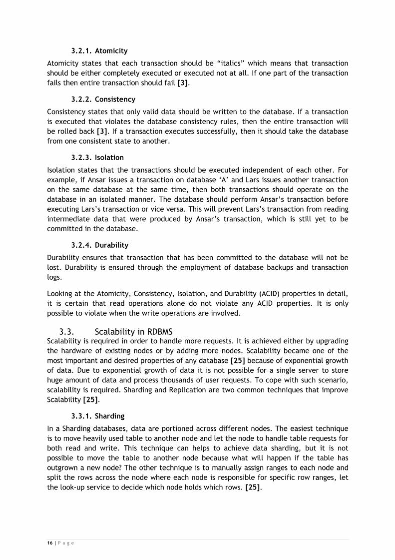
3.5.2. NOSQL Data Model
NOSQL is all about Scalability (Data Size and Data Complexity)
Figure 6- NOSQL Data Model
The Key-value store is remarkable at scaling in terms of data size, but it has weak support
for data complexity. BigTable clone is good at data size and better at data complexity
because each row can have its own schema and it does not only allow the equality queries,
rather we can also perform the range queries, and querying the specific part of the value.
Document databases are better at storing complex data and allow complex querying
efficiently. Graph databases are very good at handling data complexity.
3.6. CAP Theorem Consistency, Availability, and Partition Tolerance (CAP) was formulated by Professor
Brewer from University of California [21]. The CAP theorem states the trade off that has
to be made when designing the highly scalable systems. It lists three properties.
3.6.1. Consistency
Consistency means that querying all the nodes in the cluster should return the same data.
This means that write to one node should be replicated to all the nodes in the cluster. This
is an important feature for any distributed database system [27].
3.6.2. Availability
Availability means either the system is available or not. It guarantees that every request
receives a response.
3.6.3. Partition Tolerance
Partition Tolerance means system will continue to respond regardless of failure to
communicate within the cluster.
3.6.4. Choose any two
CAP theorem formulates that you can pick any two of the features, i.e. Consistency,
Availability, and Partition Tolerance. You cannot have three features at the same time and

22 | P a g e
get an acceptable latency. If you choose Consistency and Availability (CA) and sacrifice
partition tolerance, then your application cannot handle loss of data. In case you choose
Availability and Partition Tolerance (AP) and sacrifice consistency, then your data might
not be up-to-date in the cluster. If the third option is selected, i.e. Consistency and
Partition Tolerance (CP) while sacrificing availability, then the cluster will become
unavailable if one node is down.
3.7. Difference between RDBMS and NOSQL Database Administrators (DBAs) are defending the Relational Database Management
Systems (RDBMS) by stating that Not Only SQL (NOSQL) has no standards and it is an
immature data store [9]. NOSQL proponents react with the argument that today businesses
and organizations are generating huge amounts of data, to handle this data in an efficient
manner it should be distributed across many nodes, but RDBMS does not scale large data
volume well.
When we compare RDBMS with NOSQL, there are solid reasons for choosing RDBMS over
NOSQL as long as the schema is fixed and predefined and the amount of data is not very
large. However, there are equally good reasons for choosing NOSQL over RDBMS [9].
3.7.1. When to choose RDBMS
If you need most of the features mentioned below, then Relational Database Management
Systems (RDBMS) is definitely the right choice.
Table-Based
Referential Integrity
Atomicity, Consistency, Isolation, and Durability (ACID) Transactions
Queries and Joins
Table based nature is not the feature of RDBMS, but it is just the easiest way of storing
data in tables.
Referential Integrity is an important integrity constraint of RDBMS and it ensures the
logical consistency between the tables. Referential Integrity can also be checked at the
application layer.
The ACID properties of RDBMS ensure that either all changes that have been made are
consistent and appear the same to all users, or else none of the changes were committed.
Consistency is a property that depends on the application. For example: Will I have
concerns in case Lars is shown up married and his wife is still seen as unmarried? For the
Government yes, but for Facebook it is not.
Queries can be executed using Structured Query Language (SQL) as the query language.
SQL is more expressive than other query languages. Many Not Only SQL (NOSQL) databases
also have the abilities to execute the queries, but RDBMS queries differ from NOSQL
queries in a way that it allows group and join data from different tables into a new view.
This feature makes RDBMS a powerful tool for query execution.
23 | P a g e
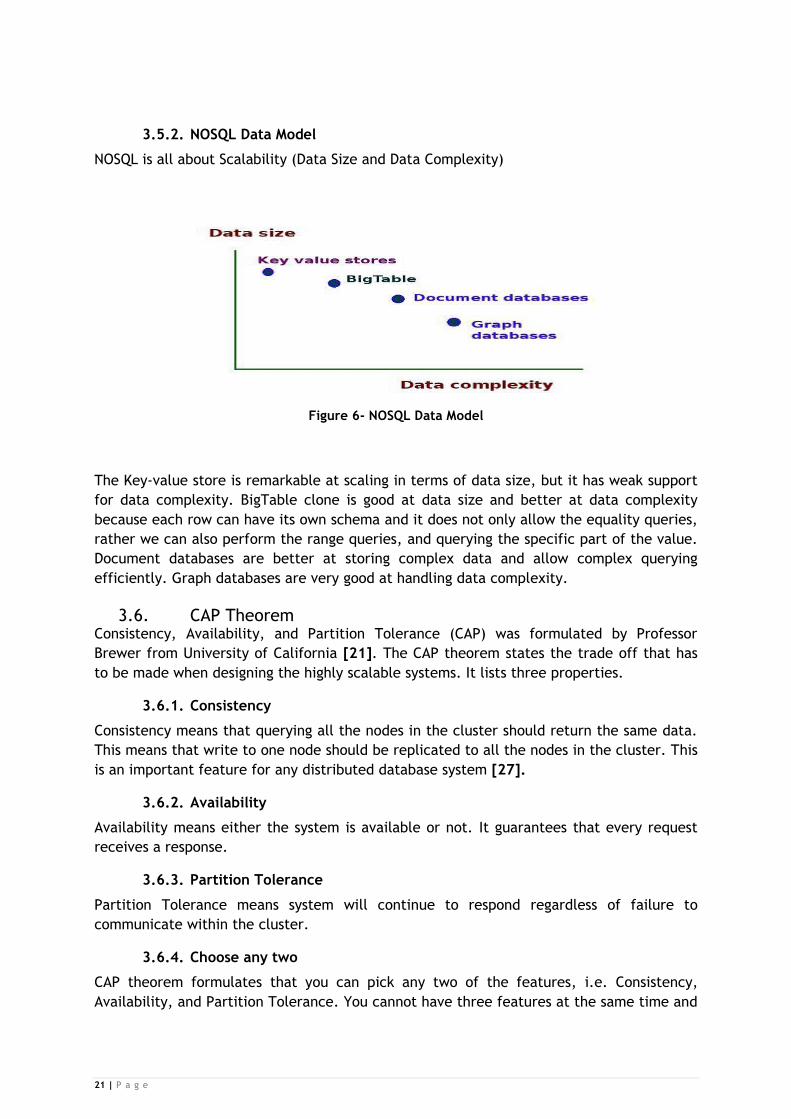
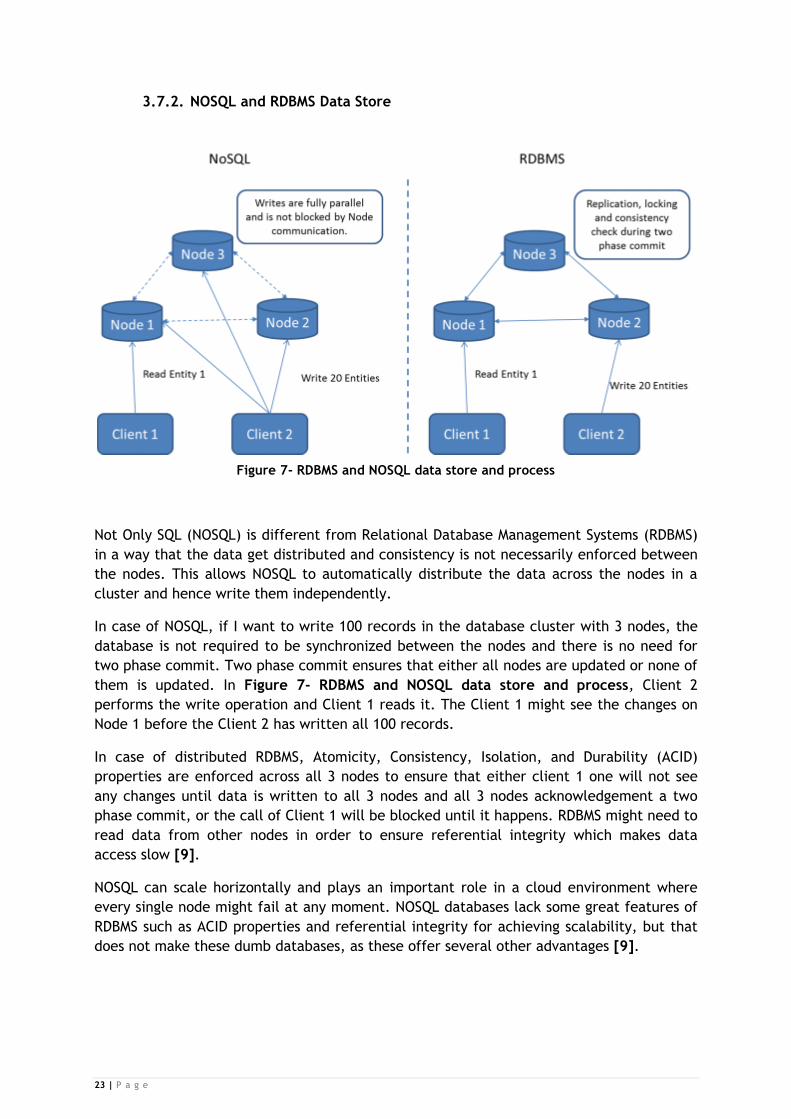
3.7.2. NOSQL and RDBMS Data Store
Figure 7- RDBMS and NOSQL data store and process
Not Only SQL (NOSQL) is different from Relational Database Management Systems (RDBMS)
in a way that the data get distributed and consistency is not necessarily enforced between
the nodes. This allows NOSQL to automatically distribute the data across the nodes in a
cluster and hence write them independently.
In case of NOSQL, if I want to write 100 records in the database cluster with 3 nodes, the
database is not required to be synchronized between the nodes and there is no need for
two phase commit. Two phase commit ensures that either all nodes are updated or none of
them is updated. In Figure 7- RDBMS and NOSQL data store and process, Client 2
performs the write operation and Client 1 reads it. The Client 1 might see the changes on
Node 1 before the Client 2 has written all 100 records.
In case of distributed RDBMS, Atomicity, Consistency, Isolation, and Durability (ACID)
properties are enforced across all 3 nodes to ensure that either client 1 one will not see
any changes until data is written to all 3 nodes and all 3 nodes acknowledgement a two
phase commit, or the call of Client 1 will be blocked until it happens. RDBMS might need to
read data from other nodes in order to ensure referential integrity which makes data
access slow [9].
NOSQL can scale horizontally and plays an important role in a cloud environment where
every single node might fail at any moment. NOSQL databases lack some great features of
RDBMS such as ACID properties and referential integrity for achieving scalability, but that
does not make these dumb databases, as these offer several other advantages [9].

24 | P a g e
3.7.3. When to choose NOSQL
If you want to store your application entities in persistent and consistent manner, so that
value is complex entity, then Relational Database Management Systems (RDBMS) is not the
right choice, however, Graph databases might be a good option.
If you have to store a large volume of data and relationships exist between the tables,
then RDBMS might not be an optimal option because large amount of data needs to be
distributed across the nodes in a cluster in order to serve multiple read/write requests for
fast storage and processing of data.
3.7.4. Why RDBMS does not scale and NOSQL does?
System scales in two ways either the nodes are upgraded or more nodes are added. If the
system handles these two conditions, then system is said to well scale and system’s
performance should increase in linear fashion. The limitation with Relational Database
Management Systems (RDBMS) is the distribution of data. Due to the limitations discussed
in Scalability in RDBMS, data Sharding and Replication are not always the right choice to
achieve scalability in RDBMS. RDBMS brings certain limitations when it comes to
distribution of data as it does not have the ability to achieve the automatic data Sharding
because it requires distinct data entities that can be easily distributed across the nodes. In
a relational database, it is very difficult to achieve because of its table-based nature.
Table based nature of relational databases make them the right choice to ensure ACID
(Atomicity, Consistency, Isolation, and Durability) properties, In contrast to this, NOSQL
(Not Only SQL) can easily distribute the rows across the nodes because of its table-less
schema and each record/entity is not distributed across multiple nodes rather whole
record/entity is stored in a single node [9].

25 | P a g e
Chapter 4
4. Analysis
This chapter discusses the nature of distributed databases and its advantages, comparison
of popular Not Only SQL (NOSQL) databases, NOSQL category selection, and NOSQL
database selection.
4.1. Distributed Database Distributed database means that data get distributed between the nodes and it has no
single physical location, instead it is distributed across a network of many nodes. It spreads
across the network of computers that are connected via communication links.
A simple distributed database architecture is shown in the figure below.
Figure 8- Distributed Databases
4.1.1. Advantages of Distributed Databases
There are numbers of advantages using NOSQL over RDBMS including:
Data Replication
26 | P a g e
Horizontally Fragmented data
Vertically Fragmented data
Improved Performance
4.1.1.1. Data Replication
Data replication means that there are multiple copies of the same data, and it is
maintained in more than one node. Data may be replicated across multiple machines to
improve data transmission between nodes. If one node goes down, then data are still
available to read from other nodes [10].
4.1.1.2. Horizontally Fragmented data
Horizontal fragmentation means that data are distributed across many nodes based on the
primary key. In horizontally fragmented data, the whole row is stored on one single node
which help reading data fast by routing the request to a specific node which owns the data
rather than routing the requests to all nodes in a cluster.
4.1.1.3. Vertically Fragmented data
Vertical fragmentation means that data has been split by columns across multiple nodes.
This helps reading the data fast if the interest is on specific column. Primary key is
replicated at each site [10].
4.1.1.4. Improved Performance
In a distributed database, performance improves depending on two basic factors.
Due to horizontal and vertical fragmentation, data get distributed across multiple
nodes to achieve scalability and each data request is sent to the closest node that
owns the data.
Due to the parallelism of distributed database systems, each query is executed in
parallel on different nodes in the network. Each query or batch is divided into sub-
queries so that many queries can be executed at the same time in order to improve
performance.
4.2. Popular NOSQL Databases Comparison Currently, there are about 122+ NOSQL databases, and it not possible to compare every
database. However, below is the comparison of popular Not Only SQL (NOSQL) databases
and their suitability according to different conditions.
4.2.1. MONGODB
MongoDB is an open source, scalable, and high performance NOSQL document-
oriented database.
It is written in C++ and provides some of the key features of SQL such as querying
and indexing.
Instead of storing data in tables, MongoDB stores JSON like documents.
It supports Ad hoc queries such as search by any field, regular expression searches,
and range queries.
It supports secondary indexes and any field can be indexed.
License: AGPL (Drivers: Apache).
27 | P a g e
Protocol: Custom, binary (BSON).
It supports master/slave replication. Read and write requests are handled by
master node while slaves node copy the data from master and only be used for data
backup or to handle the read requests.
It has a built-in sharding support which makes it to scale horizontally.
Best used: It is best used when you need dynamic and complex queries in your application
because it supports Ad hoc queries, also if you prefer to define indexes because it supports
secondary indexes and any field can indexed.
For example: MongoDB provide SQL like features such as querying and indexing so it is
best used for most of the things that you do with MySQL or PostgreSQL or any RDBMS, but
with dynamic schema instead of predefined columns [4].
4.2.2. CouchDB
CouchDB is an open source, NOSQL document database that focuses on ease to use.
It is written in Erlang.
License: Apache.
Protocol: HTTP/REST.
Unlike RDBMS, CouchDB does not store data in tables instead database is a
collection of documents.
It provides easy replication.
It uses Multiversion Concurrency Control (MVCC) to avoid database lock during write
operations.
It provides availability and partition tolerance and considered as eventually
consistent.
Best used: It is best used for the applications where data is occasionally changed or
support for versioning is important [4].
For example: Customer Relationship Management (CRM) and Content Management System
(CMS) [4].
4.2.3. Hadoop/HBase (V0.92.0)
HBase/Hadoop is an open source, non relational, and distributed database model
written in Java.
Main point: It may contain Billions of rows X millions of columns.
License: Apache.
Protocol: HTTP/REST (also Thrift).
It provides strict consistency with automatic sharding of tables.
Uses Hadoop Distributed File System (HDFS) as storage.
Map/reduce with Hadoop.
Optimizations for real-time queries.
A high performance Thrift gateway.
JRuby-based (JIRB) shell.
Rolling restarts for configuration changes and minor upgrades.
Random access performance is similar to MySQL.
28 | P a g e
It has the support of multi-site replication.
Best used: When you use the Hadoop/HDFS stack and when you need random, strict
consistency for read and write operations, and real-time read and write access to
BigTable-like data [4].
For example: For data that is similar to a search engine's data [4].
4.2.4. Apache Cassandra
Apache Cassandra is highly available, NOSQL, and distributed database management
system with Amazon Dynamo like infrastructure that is written in Java.
Main point: Best of BigTable and Dynamo with support of Billions of rows X millions
of columns.
It provides highly available services with no single point of failure.
License: Apache.
Protocol: Custom, binary (Thrift).
Consistency is tunable in Cassandra while reading or writing the data.
It supports both querying by columns and range of keys.
It provides BigTable-like features such as columns and column families.
It has a built-in secondary indexes support.
It also supports to build custom secondary indexes.
Writes are faster than reads.
It has a multi-site replication support.
Best used: When you write more than you read (logging) [4].
For example: Banking and financial industry (though not necessarily for financial
transactions, but these industries also have other needs) Writes are faster than reads [4].
4.2.5. RIAK (V1.0)
RIAK is powerful, open source, and distributed database that is written in C, Erlang,
and some Javascript.
Main point: Fault tolerance.
License: Apache.
Protocol: HTTP/REST or custom binary.
Data are distributed across nodes using consistent hashing which ensures that data
are equally distributed.
It supports secondary indexes but only one index field at a time.
It provides full-text search, indexing and querying functionality using Riak search
server.
Master-less multi-site replication and SNMP monitoring are commercially licensed.
Best used: If you want something Cassandra-like (Dynamo-like), but you are not going to
deal with complexity. If you need good single-site scalability, replication, and availability
than it is good but you have to pay for multi-site replication [4].
29 | P a g e
For example: Places where every single second is important and even seconds of
downtime can hurt, i.e Point-of-sales systems, Factory control system. [4].
4.2.6. Redis (V2.4)
Redis is open source, in memory, key-value data store that is written in C/C++.
Main point: Blazing fast.
License: BSD.
Protocol: Telnet-like.
Value in Redis can be string, but it also supports lists and sets.
It allows server side union and intersection between the sets.
It has a simple and fast Master-slave replication. To makes the master and slave
nodes up and running, only one line is required in configuration file.
Best used: For rapidly changing data with a foreseeable database size (should fit mostly in
memory). [4]
For example: Places where data gets change quickly such as Stock prices, Analytics, and
Real-time data. [4].
4.2.7. Membase
Membase is also known as Couchbase sever is a key-value data store that is written
in Erlang & C.
License: Apache 2.0.
It has peer-to-peer replication support.
It supports several languages and application frameworks.
It guarantees data consistency.
Node can easily be added or removed from a running cluster.
Write de-duplication to reduce IO.
Very nice cluster-management web GUI.
Software upgrades without taking the Database (DB) offline.
Best used: It is best used for the applications where low-latency data access and high
concurrency support is a requirement [4].
For example: Highly concurrent web apps like online gaming (e.g. Farmville) [4].
4.3. What’s wrong with Relational Database Management Systems (RDBMS)?
As such, there are no particular shortcomings of RDBMS except for the few limitations as
below:
Hard to distribute the data among nodes because of foreign key relationship
between the tables, which makes it very slow to write and process the data in the
cluster. Data Sharding requires distinct entities that can be distributed, but in
relational database it is not possible because of its table-based nature.

30 | P a g e
In RDBMS, there is no direct versioning support. Updating the record destroys the
information instead of the database adding another record with the new time
stamp when the data changes [2].
Performance falls off as RDBMS normalizes the data since normalized data requires
more tables, then denormalized data and joins between the tables. If data start to
grow in terabytes and with the growth in volume of data read and write operations
become slow down [2].
RDBMS either locks the whole table or set of records when inserting data and it
works in sequential order.
Sequential Order:
W1, W2, W3, W4, W5, and W6
RDBMS follows strict orders, which means that W1 will be performed first and W6 will be
performed at the end. For example, when inserting the record for id = 37; the database
locks all the existing records of a table. Once the last record with id=37 is inserted, then
other records are unlocked. When records are locked, no one can read or write the data
because it has been locked by another query.
The limitation with sequential approach is that it makes the database access slow. If client
1 is writing the data and gets locked, then no one can read or write the data until it is
unlocked.
Atomicity, Consistency, Isolation, and Durability (ACID) properties make it slow to
read and write the data because whenever any read or write operation is
performed on the database, RDBMS always checks that the data are consistent and
it satisfy the ACID properties.
Figure 9- Where RDBMS Stand
31 | P a g e
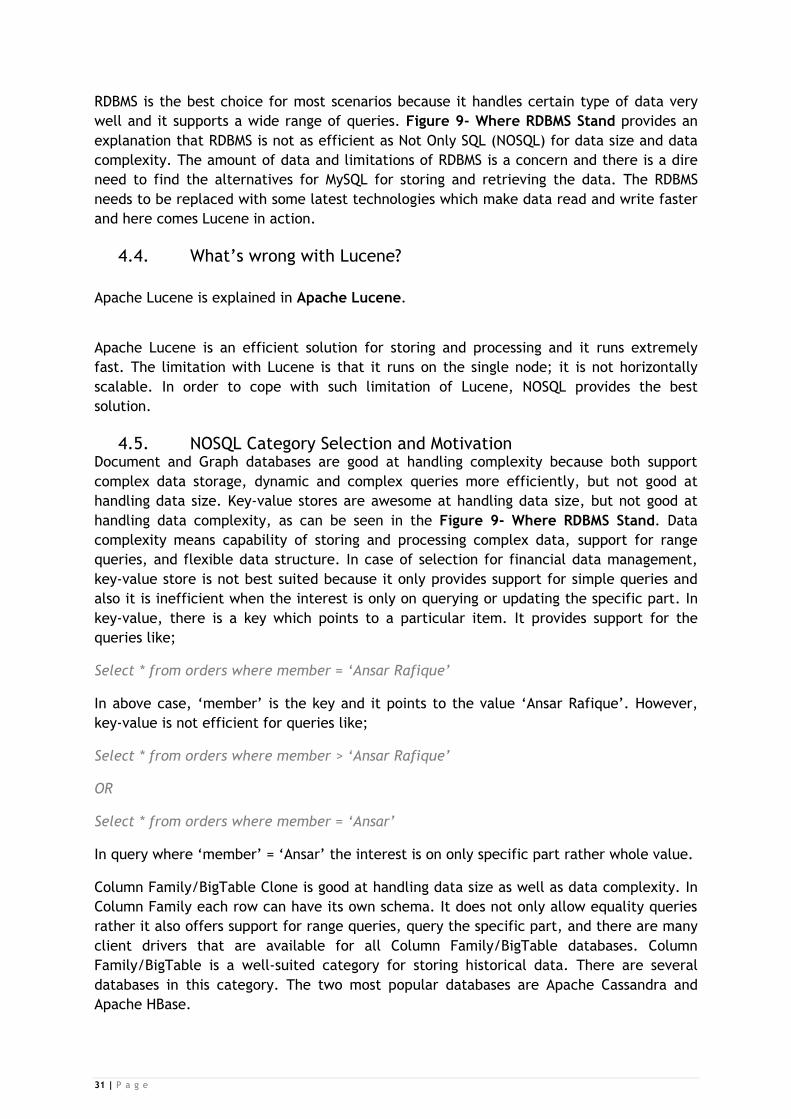
RDBMS is the best choice for most scenarios because it handles certain type of data very
well and it supports a wide range of queries. Figure 9- Where RDBMS Stand provides an
explanation that RDBMS is not as efficient as Not Only SQL (NOSQL) for data size and data
complexity. The amount of data and limitations of RDBMS is a concern and there is a dire
need to find the alternatives for MySQL for storing and retrieving the data. The RDBMS
needs to be replaced with some latest technologies which make data read and write faster
and here comes Lucene in action.
4.4. What’s wrong with Lucene?
Apache Lucene is explained in Apache Lucene.
Apache Lucene is an efficient solution for storing and processing and it runs extremely
fast. The limitation with Lucene is that it runs on the single node; it is not horizontally
scalable. In order to cope with such limitation of Lucene, NOSQL provides the best
solution.
4.5. NOSQL Category Selection and Motivation Document and Graph databases are good at handling complexity because both support
complex data storage, dynamic and complex queries more efficiently, but not good at
handling data size. Key-value stores are awesome at handling data size, but not good at
handling data complexity, as can be seen in the Figure 9- Where RDBMS Stand. Data
complexity means capability of storing and processing complex data, support for range
queries, and flexible data structure. In case of selection for financial data management,
key-value store is not best suited because it only provides support for simple queries and
also it is inefficient when the interest is only on querying or updating the specific part. In
key-value, there is a key which points to a particular item. It provides support for the
queries like;
Select * from orders where member = ‘Ansar Rafique’
In above case, ‘member’ is the key and it points to the value ‘Ansar Rafique’. However,
key-value is not efficient for queries like;
Select * from orders where member > ‘Ansar Rafique’
OR
Select * from orders where member = ‘Ansar’
In query where ‘member’ = ‘Ansar’ the interest is on only specific part rather whole value.
Column Family/BigTable Clone is good at handling data size as well as data complexity. In
Column Family each row can have its own schema. It does not only allow equality queries
rather it also offers support for range queries, query the specific part, and there are many
client drivers that are available for all Column Family/BigTable databases. Column
Family/BigTable is a well-suited category for storing historical data. There are several
databases in this category. The two most popular databases are Apache Cassandra and
Apache HBase.

32 | P a g e
4.6. NOSQL Database Selection
4.6.1. Difference between HBase and Cassandra
There is a dire need of using Distributed Scalable databases nowadays. “Big Data” is
becoming very important every day, whereas “Hadoop” has emerged as the defacto
standard for handling big data problems. Both Cassandra and HBase are influenced by
Google’s BigTable (Cassandra was directly influenced by Amazon’s Dynamo and is a hybrid
approach influenced by Amazon Dynamo and Google BigTable). BigTable stores data in
multi dimensional sorted map format.
The two databases that have gained most attentions are.
Apache Hadoop/HBase
Apache Cassandra
4.6.1.1. Apache Hadoop/HBase
HBase is a robust database for majority of use cases.
It offers strong consistency and high availability.
HBase is the part of the Hadoop eco-system. It has the support of many useful
distributed processing frameworks such as cascading and hive. Cascading is an API
which facilitates users to create solutions on Hadoop without to think about
MapReduce, but it uses MapReduce during execution. Hive is a data warehouse
system for Hadoop. Hive supports SQL like query language called HiveQL. This
makes it easier to make complex data analysis.
HBase is useful for data processing than data write.
Due to the reason it scarifies partition tolerance. HBase is a master slave
architecture, so there is a single point of failure if the master goes down.
It has the ability to handle replication up to thousands of nodes connected across
slow unpredicted internet.
A lot of configurations are required in HBase for setting nodes and clusters up and
running.
4.6.1.2. Apache Cassandra
Cassandra writes never fail, which is one of its major advantages.
It offers availability and partitioning tolerance.
Cassandra gives choice in Consistency, Availability, and Partition Tolerance (CAP).
Cassandra is useful for storing the data then processing.
It has an eventual consistency, but we can tune it to strong consistent by specifying
the consistency level while reading and writing the data.
Datastax provides a user interface which can be used to view cluster status.
It has Peer-to-Peer (P2P) structure so there is no single point of failure.
Cassandra is optimized for small data center (hundreds of nodes) connected by fast
fiber.
Little configuration is required to make the Cassandra node and cluster up and
running.
33 | P a g e
4.6.2. Motivation for Selected Database
Cassandra provides Availability and Partition Tolerance (AP). Consistency and latency are
tunable in Cassandra. Cassandra becomes eventually consistent, which means that
database can be inconsistent for a short period of time and will retrieve back its consistent
state. Strong consistency can be achieved in Cassandra by specifying a consistency level
[15]. This means that the programmer can decide whether he/she wants full consistency
among entire cluster or little inconsistency is acceptable in case the result does not
contain most up-to-date data. In contrast, HBase provides Consistency and Availability
(CA).
Both HBase and Cassandra are Apache open source products and both have their
advantages and disadvantages. Both databases are widely used these days. They differ in
data placement. The main advantage Cassandra offers over HBase is that there is no
master-slave architecture and it has no single point of failure. Cassandra requires little
configuration to make the nodes and clusters up and running which makes it a strong
candidate to select for performance benchmark test.
34 | P a g e
Chapter 5
5. Apache Cassandra – Distributed Database
This chapter discusses the most important concepts of Apache Cassandra including data
store, architecture, data partition, replication, reads and writes request, and Indexes. In-
depth detail of Cassandra can be found in DataStax documentation [23].
Apache Cassandra is a free, open source, and highly available NOSQL distributed database
system for managing huge volumes of data. Cassandra is designed to scale up to a large
size across many servers with no single point of failure.
Cassandra supports a dynamic schema data model, which provides flexibility and
performance. Cassandra uses Google Big Table data model with a Amazon Dynamo like
infrastructure with tunable consistency. The Cassandra data model is designed for large
scale distributed data to achieve performance [11]. In Cassandra both read and write
throughput increase linearly as new machines are added with no downtime and
interruption to applications [24].
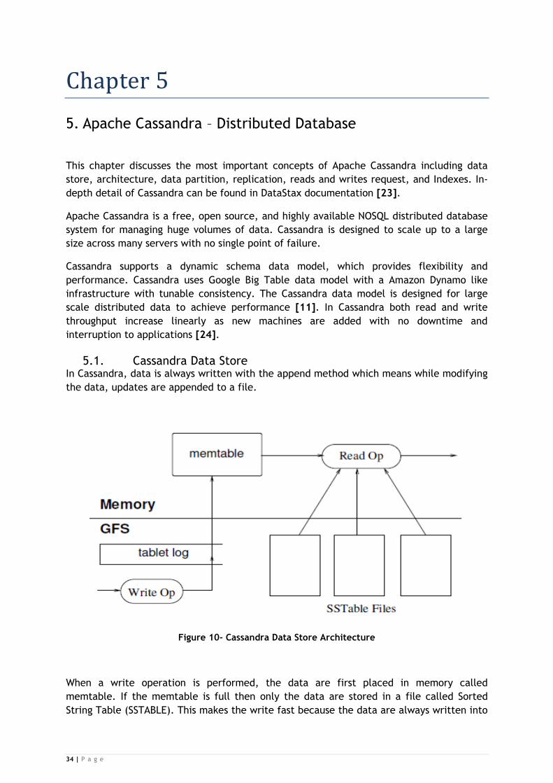
5.1. Cassandra Data Store In Cassandra, data is always written with the append method which means while modifying
the data, updates are appended to a file.
Figure 10- Cassandra Data Store Architecture
When a write operation is performed, the data are first placed in memory called
memtable. If the memtable is full then only the data are stored in a file called Sorted
String Table (SSTABLE). This makes the write fast because the data are always written into

35 | P a g e
the memtable until it gets full and thereby it avoids a great deal of Input/Output (I/O)
operations. The log file is updated every time before the data are written into memtable,
so if something goes wrong or database crashes unexpectedly, then the updated
information is available in the log file to store back and rebuilds memtable. The client
never reads the data from log file; it is only read when the node gets started for the first
time.
If a read operation is performed, initially the data are read from the memtable. If data are
not in the memtable, then data get read from SSTable. Multiple SSTables may be looked up
to find the data. Reading directly from SSTable decreases the performance because there
are many SSTable that might need to be looked at hence requires an I/O operation means
it requires touching the disk. Compared to SSTable, reading directly from memtable is fast
because there is no I/O involved. The more the I/O operations are involved, the more
performance will be degraded. Performance can also be increased by increasing the size of
memtable [7].
Cassandra uses Bloom filter to judge quickly whether the key exists in the SSTable or not
before touching the disk. Bloom filter is a efficient data structure that checks whether
element is a member of a set by dividing the memory into buckets. Check each bucket to
see if a key is present and if any bucket is empty then key was never inserted before. If
there are many SSTables, then lots of I/O operations would be needed to read the data
which can definitely decrease the performance. This is because of the fact that I/O
operations are expensive and therefore compaction is used to improve read performance.
Compaction merge two SSTables and sort to become one SSTable, which eventually
decreases the number of SSTables and number of I/O operations, hence increasing the
performance [7].
SSTable provides persistent and immutable map from keys to values. Operations are
provided to look-up the value associated with the specific key. Internally, each SSTable
contains a sequence of blocks and each block is 64 KB in size, but it is configurable [30].
Due to these reasons, read and update are slower than insert in most NOSQL databases.
5.2. Cassandra Architecture Nodes are connected to make a cluster. In Cassandra Cluster, all nodes are peers meaning
that there is no master node and no centralized management system. New node joins
Cassandra cluster based on configuration setting describe in cassandra.yaml configuration
file for each node.
5.2.1. Internodes Communication
In order to find information about the other nodes participating in the cluster, Cassandra
uses a communication protocol called gossip. Gossip is a peer-to-peer (P2P) communication
protocol. Using the gossip protocol, nodes share the information about themselves and
about the other nodes participating in the cluster [23].
In Cassandra, all nodes learn about other nodes participating in the cluster using gossip
process. The Gossip process runs to exchange the message with up to three nodes in the
cluster. The nodes share information about themselves and about other nodes they have
gossiped with [23].
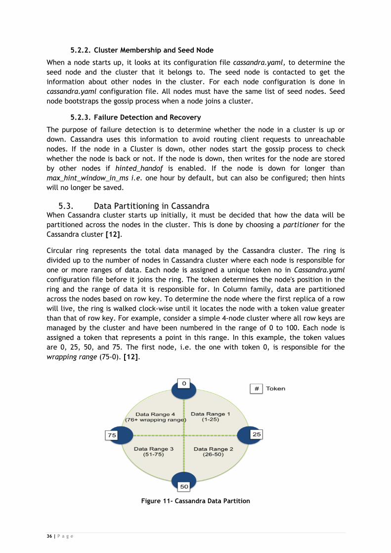
36 | P a g e
5.2.2. Cluster Membership and Seed Node
When a node starts up, it looks at its configuration file cassandra.yaml, to determine the
seed node and the cluster that it belongs to. The seed node is contacted to get the
information about other nodes in the cluster. For each node configuration is done in
cassandra.yaml configuration file. All nodes must have the same list of seed nodes. Seed
node bootstraps the gossip process when a node joins a cluster.
5.2.3. Failure Detection and Recovery
The purpose of failure detection is to determine whether the node in a cluster is up or
down. Cassandra uses this information to avoid routing client requests to unreachable
nodes. If the node in a Cluster is down, other nodes start the gossip process to check
whether the node is back or not. If the node is down, then writes for the node are stored
by other nodes if hinted_handof is enabled. If the node is down for longer than
max_hint_window_in_ms i.e. one hour by default, but can also be configured; then hints
will no longer be saved.
5.3. Data Partitioning in Cassandra When Cassandra cluster starts up initially, it must be decided that how the data will be
partitioned across the nodes in the cluster. This is done by choosing a partitioner for the
Cassandra cluster [12].
Circular ring represents the total data managed by the Cassandra cluster. The ring is
divided up to the number of nodes in Cassandra cluster where each node is responsible for
one or more ranges of data. Each node is assigned a unique token no in Cassandra.yaml
configuration file before it joins the ring. The token determines the node's position in the
ring and the range of data it is responsible for. In Column family, data are partitioned
across the nodes based on row key. To determine the node where the first replica of a row
will live, the ring is walked clock-wise until it locates the node with a token value greater
than that of row key. For example, consider a simple 4-node cluster where all row keys are
managed by the cluster and have been numbered in the range of 0 to 100. Each node is
assigned a token that represents a point in this range. In this example, the token values
are 0, 25, 50, and 75. The first node, i.e. the one with token 0, is responsible for the
wrapping range (75-0). [12].
Figure 11- Cassandra Data Partition
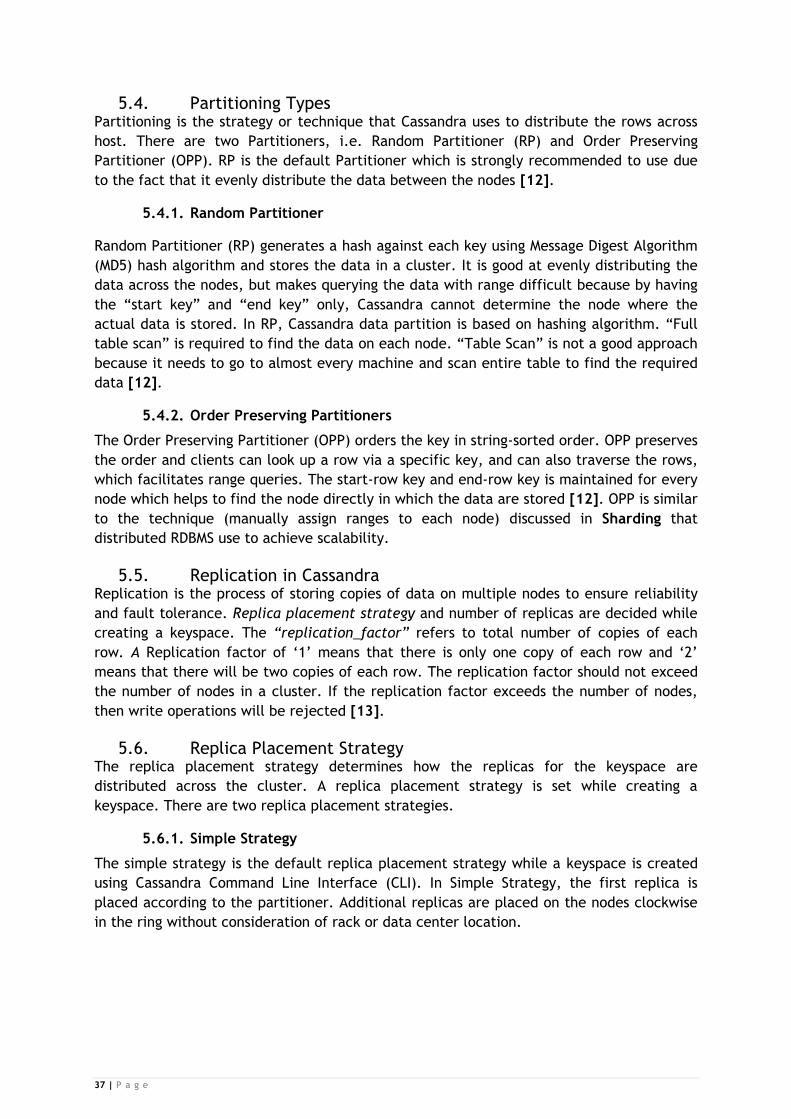
37 | P a g e
5.4. Partitioning Types Partitioning is the strategy or technique that Cassandra uses to distribute the rows across
host. There are two Partitioners, i.e. Random Partitioner (RP) and Order Preserving
Partitioner (OPP). RP is the default Partitioner which is strongly recommended to use due
to the fact that it evenly distribute the data between the nodes [12].
5.4.1. Random Partitioner
Random Partitioner (RP) generates a hash against each key using Message Digest Algorithm
(MD5) hash algorithm and stores the data in a cluster. It is good at evenly distributing the
data across the nodes, but makes querying the data with range difficult because by having
the “start key” and “end key” only, Cassandra cannot determine the node where the
actual data is stored. In RP, Cassandra data partition is based on hashing algorithm. “Full
table scan” is required to find the data on each node. “Table Scan” is not a good approach
because it needs to go to almost every machine and scan entire table to find the required
data [12].
5.4.2. Order Preserving Partitioners
The Order Preserving Partitioner (OPP) orders the key in string-sorted order. OPP preserves
the order and clients can look up a row via a specific key, and can also traverse the rows,
which facilitates range queries. The start-row key and end-row key is maintained for every
node which helps to find the node directly in which the data are stored [12]. OPP is similar
to the technique (manually assign ranges to each node) discussed in Sharding that
distributed RDBMS use to achieve scalability.
5.5. Replication in Cassandra Replication is the process of storing copies of data on multiple nodes to ensure reliability
and fault tolerance. Replica placement strategy and number of replicas are decided while
creating a keyspace. The “replication_factor” refers to total number of copies of each
row. A Replication factor of ‘1’ means that there is only one copy of each row and ‘2’
means that there will be two copies of each row. The replication factor should not exceed
the number of nodes in a cluster. If the replication factor exceeds the number of nodes,
then write operations will be rejected [13].
5.6. Replica Placement Strategy The replica placement strategy determines how the replicas for the keyspace are
distributed across the cluster. A replica placement strategy is set while creating a
keyspace. There are two replica placement strategies.
5.6.1. Simple Strategy
The simple strategy is the default replica placement strategy while a keyspace is created
using Cassandra Command Line Interface (CLI). In Simple Strategy, the first replica is
placed according to the partitioner. Additional replicas are placed on the nodes clockwise
in the ring without consideration of rack or data center location.
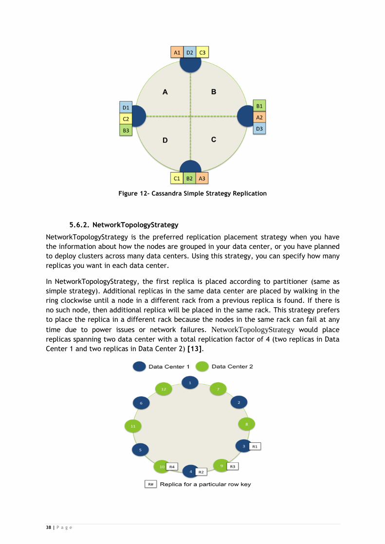
38 | P a g e
Figure 12- Cassandra Simple Strategy Replication
5.6.2. NetworkTopologyStrategy
NetworkTopologyStrategy is the preferred replication placement strategy when you have
the information about how the nodes are grouped in your data center, or you have planned
to deploy clusters across many data centers. Using this strategy, you can specify how many
replicas you want in each data center.
In NetworkTopologyStrategy, the first replica is placed according to partitioner (same as
simple strategy). Additional replicas in the same data center are placed by walking in the
ring clockwise until a node in a different rack from a previous replica is found. If there is
no such node, then additional replica will be placed in the same rack. This strategy prefers
to place the replica in a different rack because the nodes in the same rack can fail at any
time due to power issues or network failures. NetworkTopologyStrategy would place
replicas spanning two data center with a total replication factor of 4 (two replicas in Data
Center 1 and two replicas in Data Center 2) [13].
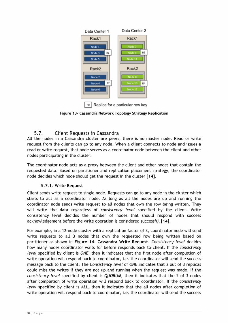
39 | P a g e
Figure 13- Cassandra Network Topology Strategy Replication
5.7. Client Requests in Cassandra All the nodes in a Cassandra cluster are peers; there is no master node. Read or write
request from the clients can go to any node. When a client connects to node and issues a
read or write request, that node serves as a coordinator node between the client and other
nodes participating in the cluster.
The coordinator node acts as a proxy between the client and other nodes that contain the
requested data. Based on partitioner and replication placement strategy, the coordinator
node decides which node should get the request in the cluster [14].
5.7.1. Write Request
Client sends write request to single node. Requests can go to any node in the cluster which
starts to act as a coordinator node. As long as all the nodes are up and running the
coordinator node sends write request to all nodes that own the row being written. They
will write the data regardless of consistency level specified by the client. Write
consistency level decides the number of nodes that should respond with success
acknowledgement before the write operation is considered successful [14].
For example, in a 12-node cluster with a replication factor of 3, coordinator node will send
write requests to all 3 nodes that own the requested row being written based on
partitioner as shown in Figure 14- Cassandra Write Request. Consistency level decides
how many nodes coordinator waits for before responds back to client. If the consistency
level specified by client is ONE, then it indicates that the first node after completion of
write operation will respond back to coordinator, i.e. the coordinator will send the success
message back to the client. The Consistency level of ONE indicates that 2 out of 3 replicas
could miss the writes if they are not up and running when the request was made. If the
consistency level specified by client is QUORUM, then it indicates that the 2 of 3 nodes
after completion of write operation will respond back to coordinator. If the consistency
level specified by client is ALL, then it indicates that the all nodes after completion of
write operation will respond back to coordinator, i.e. the coordinator will send the success
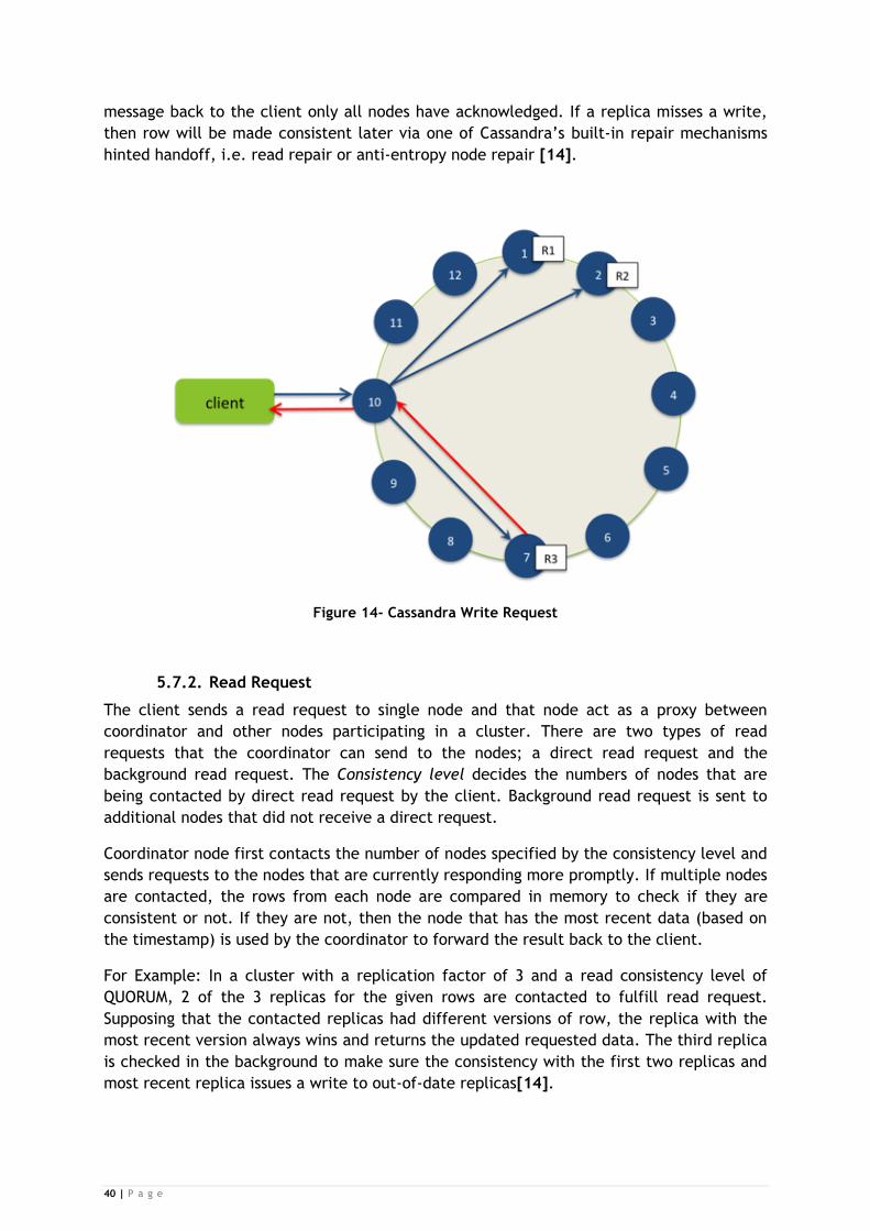
40 | P a g e
message back to the client only all nodes have acknowledged. If a replica misses a write,
then row will be made consistent later via one of Cassandra’s built-in repair mechanisms
hinted handoff, i.e. read repair or anti-entropy node repair [14].
Figure 14- Cassandra Write Request
5.7.2. Read Request
The client sends a read request to single node and that node act as a proxy between
coordinator and other nodes participating in a cluster. There are two types of read
requests that the coordinator can send to the nodes; a direct read request and the
background read request. The Consistency level decides the numbers of nodes that are
being contacted by direct read request by the client. Background read request is sent to
additional nodes that did not receive a direct request.
Coordinator node first contacts the number of nodes specified by the consistency level and
sends requests to the nodes that are currently responding more promptly. If multiple nodes
are contacted, the rows from each node are compared in memory to check if they are
consistent or not. If they are not, then the node that has the most recent data (based on
the timestamp) is used by the coordinator to forward the result back to the client.
For Example: In a cluster with a replication factor of 3 and a read consistency level of
QUORUM, 2 of the 3 replicas for the given rows are contacted to fulfill read request.
Supposing that the contacted replicas had different versions of row, the replica with the
most recent version always wins and returns the updated requested data. The third replica
is checked in the background to make sure the consistency with the first two replicas and
most recent replica issues a write to out-of-date replicas[14].

41 | P a g e
Figure 15- Cassandra Read Request
5.8. Indexes in Cassandra Indexes allow the fast and efficient look-up of data.
5.8.1. Primary Index
The primary key is a unique key that is used to identify each row in a table. In Cassandra,
the primary index for a column family is its row key. Each node in the cluster maintains
the primary index for the data it contains.
5.8.2. Alternate Index
Secondary Index is a way to find rows through other means than row keys. A secondary
Index is an index on the column values. Cassandra supports secondary index of type KEYS.
KEYS is similar to a hash index and Cassandra secondary indexes allows for efficient
querying by using equality predicates (where a = b). Cassandra uses the term “secondary
index” to refer to the native secondary index (built-in) support that was added to version
0.7. Alternate index is a broader term, which refers to both native secondary index (built-
in) secondary index and techniques to create custom indexes in Cassandra.
5.8.3. Native Secondary Indexes (Built-in)
Cassandra's built-in secondary index is the best choice for cases when many rows contain
the same column value for a particular column. The more unique values there exist in a
particular column, the more overhead there will be to maintain the index [20]. For
example, suppose you have a user table with millions of users and you are interested in
looking up users by state. Many users will share the same column value for the state (such
as Stockholm, Uppsala, Blekinge, and Kalmar). This would be a good candidate for a
secondary index. On the other hand, if you want to look up users by their email address,
42 | P a g e
then email address is unique for each user, and it will be more efficient to build a custom
secondary index on user and maintain a dynamic column family as a form of an "index".
5.8.4. Build Custom Secondary Index
There are different techniques to create your custom secondary indexes in Cassandra. If
you are using random partitioner for the equal distribution of data among the nodes in a
cluster, and you want to have the range query facility, then you might need to build
custom secondary index. In case of random partitioner is used it is not easy to traverse row
keys because by having only the “start key” and “end key” Cassandra cannot determine
the node where the actual data is stored, also the sorting order of those keys is based on
hashing algorithm. This technique allows performing the range queries.
5.8.5. Use Secondary Index
In order to create a secondary index you can either specify the KEYS index type when
creating a column family or you can add it later to existing column family. Secondary
indexes are automatically built in the background without blocking read or write
operations.
5.8.5.1. Create New Column Family with Index
Column family in Cassandra is similar to table in RDBMS where the actual data is stored.
Below is an example of creating secondary index of type KEYS while creating a new column
family. Secondary index is created on column state where index_type is KEYS.
Create column family users with comparator=UTF8Type and column_metadata=[{column_name: full_name, validation_class: UTF8Type}, {column_name: email, validation_class: UTF8Type}, {column_name: birth_year, validation_class: LongType, index_type: KEYS}, {column_name: state, validation_class: UTF8Type, index_type: KEYS}];
5.8.5.2. Create Index on existing column family
Cassandra also allows create indexes on existing column families. Secondary indexes on
existing column families are built in the background without blocking reads and writes
operations. Below is an example of creating secondary index of type KEYS on existing
column family. Secondary index is created on column state where index_type is KEYS.
update column family users with comparator=UTF8Type and column_metadata=[{column_name: full_name, validation_class: UTF8Type}, {column_name: email, validation_class: UTF8Type}, {column_name: birth_year, validation_class: LongType, index_type: KEYS}, {column_name: state, validation_class: UTF8Type, index_type: KEYS}];
An Index has been created on a column state so it can be directly queried using
get users where state = ' Uppsala’;
5.9. How Cassandra differs from RDBMS Instead of building on a relational model, the team behind Cassandra identified the
limitations that exist with Relational Databases Management Systems (RDBMS) and how
43 | P a g e
these limitations can be solved. Cassandra has taken a completely different approach for
database design than RDBMS [25].
From an architect perspective, the core difference between Cassandra and RDBMS is data
modeling. In RDBMS the main focus is mostly on the data store and data relationship while
in Cassandra the main focus is on how the data will be accessed [25].
From an operational team’s point of view, it is very easy to add or remove nodes in
Cassandra cluster, which is not in the case of RDBMS [25].
5.10. Tuning Cassandra for Improving Performance Cassandra can be tuned to improve the performance for both read and write.
5.10.1. Improve writes performance
Cassandra is extremely fast for writing the data, but still writing performance can
significantly be improved in Cassandra by tuning the following parameters.
In order to maximize write performance, it is recommended to use a separate hard disk for
the data file and commit log, so the data file and commit log are not competing for
Input/Output (I/O) bandiwidth. These configurations can be configured in cassandra.yaml
configuration file.
commitlog_directory: /var/lib/cassandra/commitlog data_file_directories: /var/lib/cassandra/data
Cassandra, like many other databases, is dependent on the speed of hard disk and
speed of Central Processing Units (CPUs). It is recommended using the fastest disks
and four or eight cores CPUs to take the advantage of Cassandra high concurrency.
Instead of using wrapper over Remote Procedure Calls (RPC) client, direct use of
fast RPC client can also increase write performance.
Decreasing Write Consistency Level also help increasing write performance, as
fewer nodes need to be blocked for write operations.
5.10.2. Improve read performance
Cassandra read performance is not as efficient as write performance because it is a write-
oriented system; [24] but it can be enhanced by tuning a couple of parameters.
Key caching and/or Row caching can be enabled in Cassandra to improve read
performance.
By default key cache is enabled and Cassandra caches 20,000 keys per Column
Family (CF). The key cache decreases the Input/Output (I/O) operations because if
key cache is not enabled then I/O operation is required in order to figure out the
exact location of the row. Key cache holds the exact location of the data belonging
to that key.
Row cache holds the entire content of the row in cache. By default, row cache is
disabled. The overhead of enabling or increasing the row cache is that it may
require more Java Virtual Machine (JVM) heap of Cassandra.
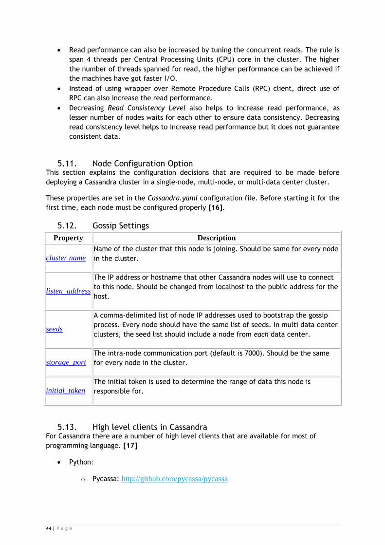
44 | P a g e
Read performance can also be increased by tuning the concurrent reads. The rule is
span 4 threads per Central Processing Units (CPU) core in the cluster. The higher
the number of threads spanned for read, the higher performance can be achieved if
the machines have got faster I/O.
Instead of using wrapper over Remote Procedure Calls (RPC) client, direct use of
RPC can also increase the read performance.
Decreasing Read Consistency Level also helps to increase read performance, as
lesser number of nodes waits for each other to ensure data consistency. Decreasing
read consistency level helps to increase read performance but it does not guarantee
consistent data.
5.11. Node Configuration Option This section explains the configuration decisions that are required to be made before
deploying a Cassandra cluster in a single-node, multi-node, or multi-data center cluster.
These properties are set in the Cassandra.yaml configuration file. Before starting it for the
first time, each node must be configured properly [16].
5.12. Gossip Settings
Property Description
cluster name
Name of the cluster that this node is joining. Should be same for every node
in the cluster.
listen_address
The IP address or hostname that other Cassandra nodes will use to connect
to this node. Should be changed from localhost to the public address for the
host.
seeds
A comma-delimited list of node IP addresses used to bootstrap the gossip
process. Every node should have the same list of seeds. In multi data center
clusters, the seed list should include a node from each data center.
storage_port
The intra-node communication port (default is 7000). Should be the same
for every node in the cluster.
initial_token
The initial token is used to determine the range of data this node is
responsible for.
5.13. High level clients in Cassandra For Cassandra there are a number of high level clients that are available for most of
programming language. [17]
Python:
o Pycassa: http://github.com/pycassa/pycassa

45 | P a g e
o Telephus: http://github.com/driftx/Telephus (Twisted)
Java:
o Astyanax: https://github.com/Netflix/astyanax/wiki/Getting-Started
o CQL-JDBC:
Site: http://code.google.com/a/apache-extras.org/p/cassandra-jdbc/
Sources: http://code.google.com/a/apache-extras.org/p/cassandra-
jdbc/source/checkout
Hector:
o Site: http://hector-client.org
o Examples https://github.com/zznate/hector-examples
o Sources http://github.com/rantav/hector
Kundera http://github.com/impetus-opensource/Kundera
o Examples https://github.com/impetus-opensource/Kundera-Examples
Pelops: http://github.com/s7/scale7-pelops
Easy-Cassandra: https://github.com/otaviojava/Easy-Cassandra
o Cassandrelle (Demoiselle Cassandra):
http://demoiselle.sf.net/component/demoiselle-cassandra/
o User guide: http://demoiselle.sourceforge.net/docs/guide-cassandra/
Scala
o Cascal: https://github.com/Shimi/cascal
o Cassie: https://github.com/twitter/cassie
Node.js
o Helenus: https://github.com/simplereach/helenus
Clojure
o clj-hector: https://github.com/pingles/clj-hector
.NET
o Aquiles: http://aquiles.codeplex.com/
o Cassandraemon: http://cassandraemon.codeplex.com/

46 | P a g e
o cassandra-sharp: http://code.google.com/p/cassandra-sharp/
o FluentCassandra: https://github.com/managedfusion/fluentcassandra
Ruby:
o Fauna: https://github.com/twitter/cassandra
PHP:
o Cassandra PHP Client Library: https://github.com/kallaspriit/Cassandra-PHP-
Client-Library
o phpcassa: http://github.com/thobbs/phpcassa
o SimpleCassie: http://code.google.com/p/simpletools-php/wiki/SimpleCassie
o Pandra: https://github.com/mjpearson/Pandra
Perl:
o Cassandra::Simple: https://github.com/fmgoncalves/p5-cassandra-simple
o Net::Cassandra: http://search.cpan.org/~lbrocard/Net-Cassandra-
0.35/lib/Net/Cassandra.pm
o Net::Cassandra::Easy: http://search.cpan.org/~teodor/Net-Cassandra-Easy-
0.15/
o Cassandra::Lite: http://search.cpan.org/~gslin/Cassandra-Lite-0.4.0/
C++
o libQtCassandra repository: http://sf.net/p/libqtcassandra/
o Home Page, Developer Guide: http://snapwebsites.org/project/libqtcassandra
Haskell
o cassy: https://github.com/ozataman/cassy
o HackageDB Page: http://hackage.haskell.org/package/cassy
47 | P a g e
Chapter 6
6. Implementation Environment
Performance benchmark implementation for MySQL, Apache Cassandra, and Apache Lucene
has been done using various Java technologies. The purpose of implementation is to find
out the throughput for selected set of technologies. For the backend permanent data
storage MySQL, Apache Cassandra and Apache Lucene are used. The ultimate purpose is to
find out how different databases behave for different variants with different amount of
data in the database.
For most of the development work, Eclipse is used as an Integrated Development
Environment (IDE) and Swing Application Programming Interface (API) for the interface
design.
6.1. Java Java is the programming language and platform first released by Sun Microsystems in 1995
and it is one of the most popular programming languages today. It is an object-oriented
language that derives most of its syntax from C++, but it has a simpler object model.
Java program is compiled to byte code (class file) called Java Byte Code (JBC). JBC can run
on any Java Virtual Machine (JVM) regardless of computer architecture. Java is intended to
“write once run anywhere”; means that code runs on one platform and has does not need
to be recompiled in order to run on another platform.
Java comes in three flavors:
6.1.1. Java to Standard Edition (J2SE)
J2SE contains mixed general purpose libraries including Java Database Connectivity (JDBC),
Java Naming Directory Interface (JNDI), Remote Method Invocation (RMI), Abstract Window
Toolkit (AWT), and Swing.
6.1.2. Java Enterprise Edition (Java EE)
JavaEE known as Java to Enterprise Edition (J2EE), it includes Java to Standard Edition
(J2SE) plus most of other Java technologies; few of which are Java Mail, Java Server Pages
(JSP), Servlets, Enterprise Java Beans (EJB), and Java Server Faces (JSF).
6.1.3. Java Micro Edition (Java ME)
JavaME known as Java to Micro Edition (J2ME), it includes most of the Java to Standard
Edition (J2SE) and some additional Application Programming Interfaces (APIs) for devices.
The Implementation is done using J2SE flavor.
All the development for the project was done using Java, and the Swing library was used to
create an interface for the application that generates benchmark graphs.
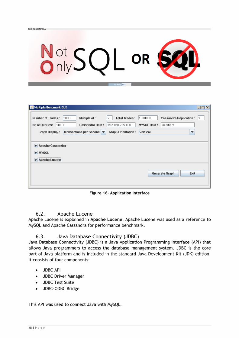
48 | P a g e
Figure 16- Application Interface
6.2. Apache Lucene Apache Lucene is explained in Apache Lucene. Apache Lucene was used as a reference to
MySQL and Apache Cassandra for performance benchmark.
6.3. Java Database Connectivity (JDBC) Java Database Connectivity (JDBC) is a Java Application Programming Interface (API) that
allows Java programmers to access the database management system. JDBC is the core
part of Java platform and is included in the standard Java Development Kit (JDK) edition.
It consists of four components:
JDBC API
JDBC Driver Manager
JDBC Test Suite
JDBC-ODBC Bridge
This API was used to connect Java with MySQL.

49 | P a g e
Figure 17- JDBC Connectivity
MYSQLJDBCConnector
The class below connects Java with MySQL and returns the connection object for the
execution of statement. This class implements the singleton pattern, i.e. it does not
always create abcCon object when calls come to this method. It only creates the object, if
abcCon is null or it is closed.
package com.cinnober.framework.mysql.jdbc.connection;
import java.sql.*;
import com.cinnober.framework.mysql.jdbc.config.MYSQLConfig;
/**
* JDBC Connector to create connection between Java and MYSQL
* @author ansar.rafique
*
*/
public class MYSQLJDBCConnector {
private static Connection abcCon = null;
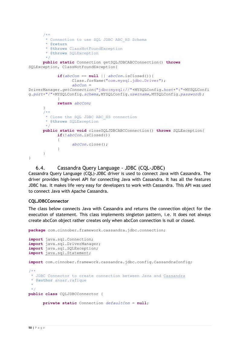
50 | P a g e
/**
* Connection to use SQL JDBC ABC_HS Schema
* @return
* @throws ClassNotFoundException
* @throws SQLException
*/
public static Connection getSQLJDBCABCConnection() throws
SQLException, ClassNotFoundException{
if(abcCon == null || abcCon.isClosed()){
Class.forName("com.mysql.jdbc.Driver");
abcCon =
DriverManager.getConnection("jdbc:mysql://"+MYSQLConfig.host+":"+MYSQLConfi
g.port+"/"+MYSQLConfig.schema,MYSQLConfig.username,MYSQLConfig.password);
}
return abcCon;
}
/**
* Close the SQL JDBC ABC_HS connection
* @throws SQLException
*/
public static void closeSQLJDBCABCConnection() throws SQLException{
if(!abcCon.isClosed())
{
abcCon.close();
}
}
}
6.4. Cassandra Query Language - JDBC (CQL-JDBC) Cassandra Query Language (CQL)-JDBC driver is used to connect Java with Cassandra. The
driver provides high-level API for connecting Java with Cassandra. It has all the features
JDBC has. It makes life very easy for developers to work with Cassandra. This API was used
to connect Java with Apache Cassandra.
CQLJDBCConnector
The class below connects Java with Cassandra and returns the connection object for the
execution of statement. This class implements singleton pattern, i.e. It does not always
create abcCon object rather creates only when abcCon connection is null or closed.
package com.cinnober.framework.cassandra.jdbc.connection;
import java.sql.Connection;
import java.sql.DriverManager;
import java.sql.SQLException;
import java.sql.Statement;
import com.cinnober.framework.cassandra.jdbc.config.CassandraConfig;
/**
* JDBC Connector to create connection between Java and Cassandra
* @author ansar.rafique
*
*/
public class CQLJDBCConnector {
private static Connection defaultCon = null;
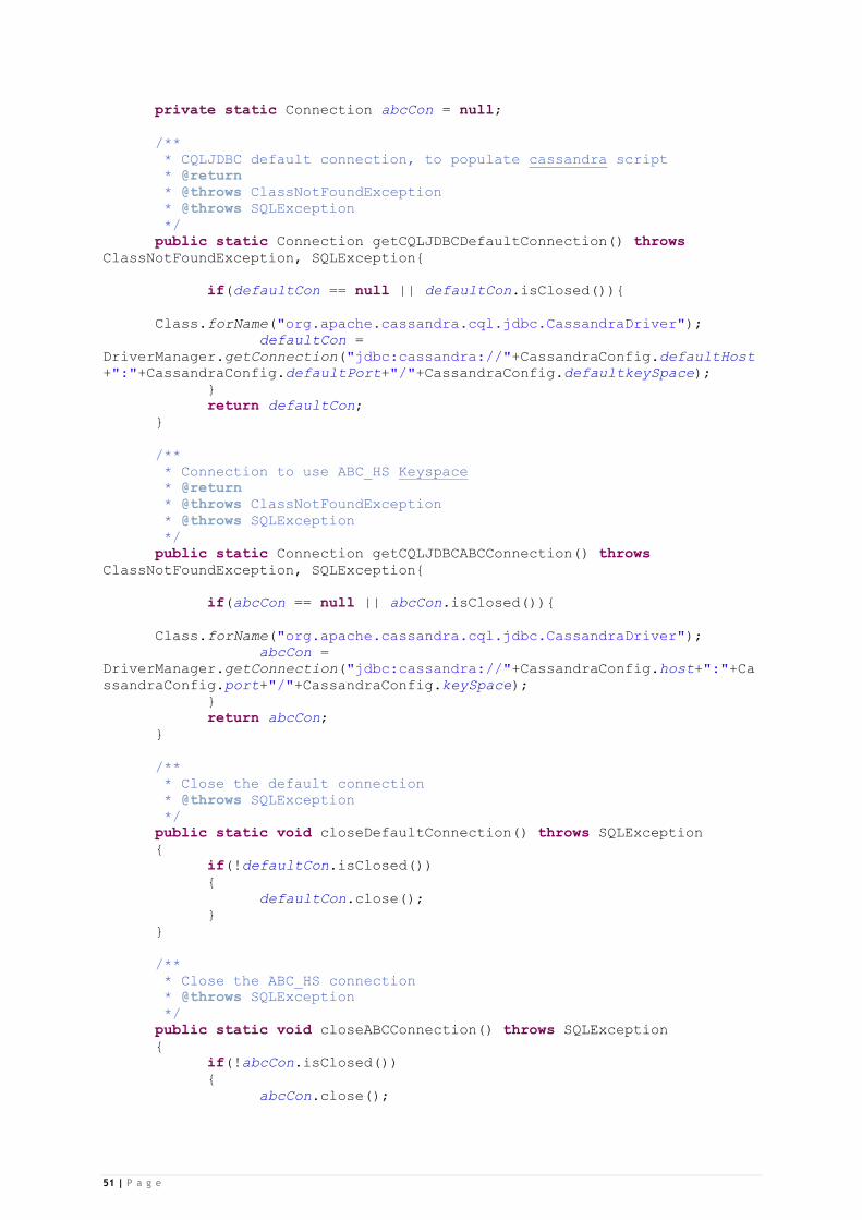
51 | P a g e
private static Connection abcCon = null;
/**
* CQLJDBC default connection, to populate cassandra script
* @return
* @throws ClassNotFoundException
* @throws SQLException
*/
public static Connection getCQLJDBCDefaultConnection() throws
ClassNotFoundException, SQLException{
if(defaultCon == null || defaultCon.isClosed()){
Class.forName("org.apache.cassandra.cql.jdbc.CassandraDriver");
defaultCon =
DriverManager.getConnection("jdbc:cassandra://"+CassandraConfig.defaultHost
+":"+CassandraConfig.defaultPort+"/"+CassandraConfig.defaultkeySpace);
}
return defaultCon;
}
/**
* Connection to use ABC_HS Keyspace
* @return
* @throws ClassNotFoundException
* @throws SQLException
*/
public static Connection getCQLJDBCABCConnection() throws
ClassNotFoundException, SQLException{
if(abcCon == null || abcCon.isClosed()){
Class.forName("org.apache.cassandra.cql.jdbc.CassandraDriver");
abcCon =
DriverManager.getConnection("jdbc:cassandra://"+CassandraConfig.host+":"+Ca
ssandraConfig.port+"/"+CassandraConfig.keySpace);
}
return abcCon;
}
/**
* Close the default connection
* @throws SQLException
*/
public static void closeDefaultConnection() throws SQLException
{
if(!defaultCon.isClosed())
{
defaultCon.close();
}
}
/**
* Close the ABC_HS connection
* @throws SQLException
*/
public static void closeABCConnection() throws SQLException
{
if(!abcCon.isClosed())
{
abcCon.close();
52 | P a g e
}
}
}
6.5. JUNIT JUnit is the unit test framework for Java programming language. Java is important in test-
driven-development and it is one of the families of unit test framework. This API was used
for Java benchmark testing.
6.6. JFreeChart JFreeChart is a free and open source Java chart library that makes it easy for developers
to display the charts in the application. This API was used to create charts and display the
benchmark test in the charts.
6.7. MySQL MySQL is the RDBMS that is used to store the data in tables. It supports a query language
called SQL. MySQL was used to store the relational data in the database.
6.8. Apache Cassandra Cassandra is explained in Apache Cassandra – Distributed Database. Cassandra is used for
most of the implementation. It is a core part of the thesis. Cassandra is used to stored data
on single node and 3-node cluster using replication factor up to 1, 2, and 3.

53 | P a g e
Chapter 7
7. Testing and Evaluation
As described in Research Background about the History Server (HS). Along with HS there is
another server called Query Server (QS). Both HS and QS store orders. HS store trades and
orders for a long period of time and responds to queries. Each trade and order contain at
least order id, sequence number, time of event, order book, trading member, member,
and user where each user belongs to a single member. Each trade and order has number of
attributes, but I have assumed that order id, member, user, and member and user
attribute will gain access frequently so secondary indexes are created on selected columns
to make the data access fast. The goal is to experiment with different databases with
different indexing strategies to examine the behavior and read and write throughput for
different data sets. For performance benchmark, three popular selected databases are
MySQL, Apache Cassandra, and Apache Lucene.
For MySQL, the variants are no-index, user-index, and member & user-index. For MySQL,
in case of no-index, it will go through the entire table to match the conditions and full
table scan is required, in case of user-index, secondary index is created on the user column
for quick search. If a user is involved in any conditional query then it will retrieve the user
data fast because MySQL maintains the index for secondary indexes and it doesn’t need to
go through the entire table. In case of member & user-index, index is created on tuple,
which is the combination of member & user. If member & user are involved in any
conditional query then it will retrieve the data fast as it maintains the index for secondary
indexes.
For Apache Cassandra, the variants are no-index, user-index, member-index & user-index,
and a custom-index (user). For reading the data in case of no-index, all the records need
to be fetched in order to match the elements programmatically because Cassandra does
not support the conditional query on non-key columns until and unless there is at least one
secondary index. For Cassandra, in case of member-index & user-index, it is different from
MySQL index because Cassandra does not allow the index on tuple; separate index is
created on both columns. In case of custom-index on user, I have built a custom secondary
index on the user column by using the pattern (one-to-many) keeping random partitioner
as the default for an equal distribution of data. New hidden column, i.e. family user; is
created for the indexed column values and all the column values become a single row with
only one KEY having many columns. This technique helps perform the range queries on the
column because all the columns in a row are sorted by default if the value of comparator is
specified.
For Apache Lucene, the variants are user-index and member & user-index. For Lucene, in
case of user-index an index is created on the user column and in case of member & user-
index, index is created on combination of both columns.
Building a good performance benchmark model for Cassandra requires a deep
understanding of its architecture, data storage, and data distribution mechanism. Taking
all this information into account, I have built a performance benchmark test which
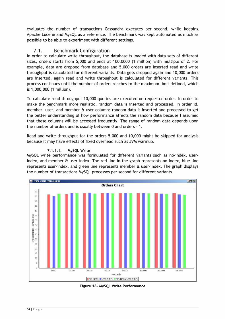
54 | P a g e
evaluates the number of transactions Cassandra executes per second, while keeping
Apache Lucene and MySQL as a reference. The benchmark was kept automated as much as
possible to be able to experiment with different settings.
7.1. Benchmark Configuration In order to calculate write throughput, the database is loaded with data sets of different
sizes, orders starts from 5,000 and ends at 100,0000 (1 million) with multiple of 2. For
example, data are dropped from database and 5,000 orders are inserted read and write
throughput is calculated for different variants. Data gets dropped again and 10,000 orders
are inserted, again read and write throughput is calculated for different variants. This
process continues until the number of orders reaches to the maximum limit defined, which
is 1,000,000 (1 million).
To calculate read throughput 10,000 queries are executed on requested order. In order to
make the benchmark more realistic, random data is inserted and processed. In order id,
member, user, and member & user columns random data is inserted and processed to get
the better understanding of how performance affects the random data because I assumed
that these columns will be accessed frequently. The range of random data depends upon
the number of orders and is usually between 0 and orders – 1.
Read and write throughput for the orders 5,000 and 10,000 might be skipped for analysis
because it may have effects of fixed overhead such as JVM warmup.
7.1.1.1. MySQL Write
MySQL write performance was formulated for different variants such as no-index, user-
index, and member & user-index. The red line in the graph represents no-index, blue line
represents user-index, and green line represents member & user-index. The graph displays
the number of transactions MySQL processes per second for different variants.
Figure 18- MySQL Write Performance
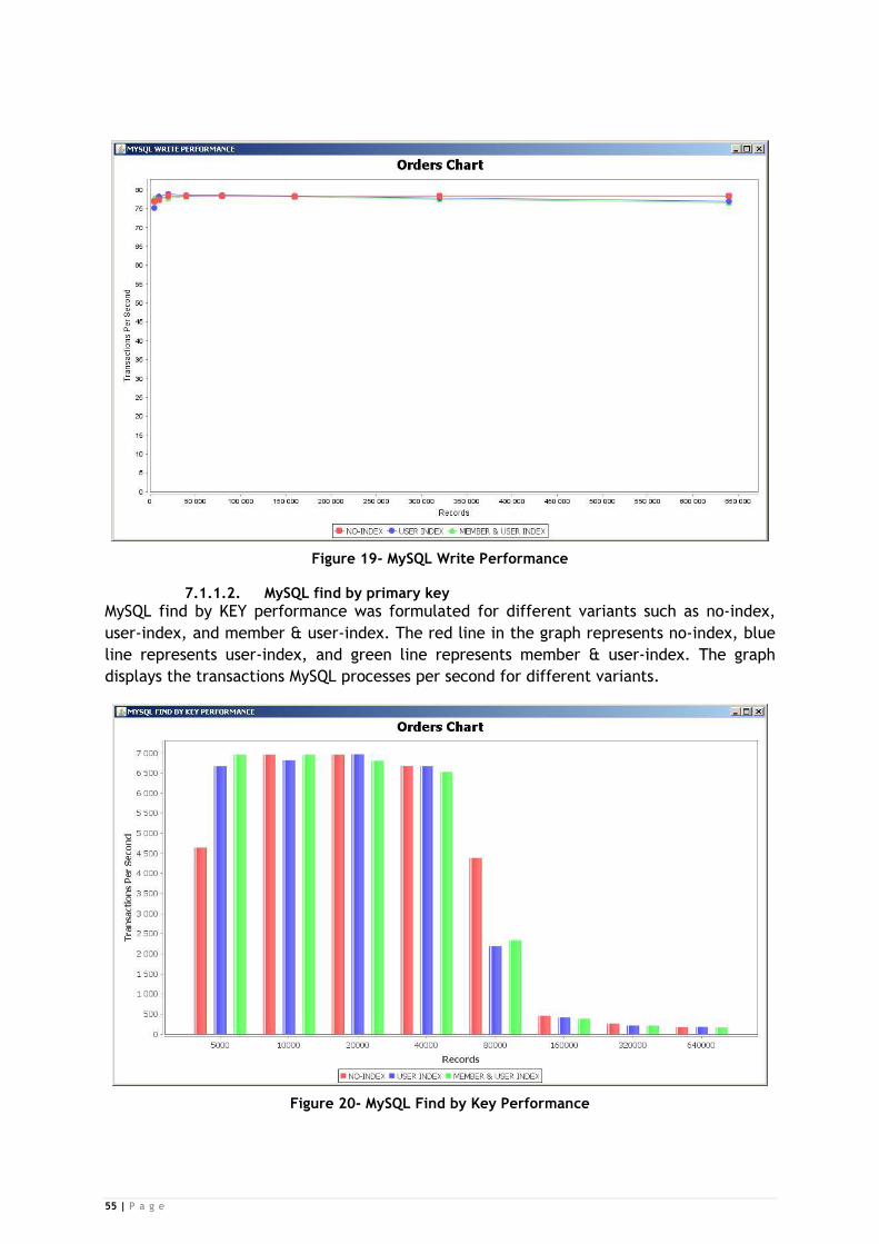
55 | P a g e
Figure 19- MySQL Write Performance
7.1.1.2. MySQL find by primary key
MySQL find by KEY performance was formulated for different variants such as no-index,
user-index, and member & user-index. The red line in the graph represents no-index, blue
line represents user-index, and green line represents member & user-index. The graph
displays the transactions MySQL processes per second for different variants.
Figure 20- MySQL Find by Key Performance

56 | P a g e
Figure 21- MySQL Find by Key Performance
7.1.1.3. MySQL find by parameters
MySQL find by parameters performance was formulated for different different variants
such as no-index, user-index, and member & user-index. The red line in the graph
represents no-index, blue line represents user-index, and green line represents member &
user-index. The graph displays the transactions MySQL processes per second for different
variants.
Figure 22- MySQL Find by Parameter Performance
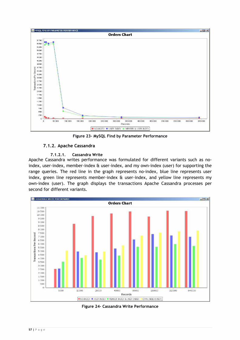
57 | P a g e
Figure 23- MySQL Find by Parameter Performance
7.1.2. Apache Cassandra
7.1.2.1. Cassandra Write
Apache Cassandra writes performance was formulated for different variants such as no-
index, user-index, member-index & user-index, and my own-index (user) for supporting the
range queries. The red line in the graph represents no-index, blue line represents user
index, green line represents member-index & user-index, and yellow line represents my
own-index (user). The graph displays the transactions Apache Cassandra processes per
second for different variants.
Figure 24- Cassandra Write Performance

58 | P a g e
Figure 25- Cassandra Write Performance
7.1.2.2. Cassandra find by key
Apache Cassandra finds by KEY performance was formulated for different variants such as
no-index, user-index, member-index & user-index, and my own-index (user). The red line
in the graph represents no-index, blue line represents user-index, green line represents
member-index & user-index, and yellow line represents my own-index (user). The graph
displays the transactions Apache Cassandra processes per second for different variants.
Figure 26- Cassandra Find by Key Performance

59 | P a g e
Figure 27- Cassandra Find by Key Performance
7.1.2.3. Cassandra find by parameters
Apache Cassandra finds by parameters performance was formulated for different variants
such as no-index, user-index, member-index & user-index, and my own-index (user). The
red line in the graph represents no-index, blue line represents user-index, green line
represents member-index & user index, and yellow line represents my own-index (user).
The graph displays the transactions Apache Cassandra processes per second for different
variants.
Figure 28- Cassandra Find by Parameter Performance

60 | P a g e
Figure 29- Cassandra Find by Parameter Performance
7.1.3. Apache Lucene
7.1.3.1. Lucene Write
Apache Lucene writes performance was formulated for variants such as user-index and
member & user-index. The red line in the graph represents user-index and blue line
represents member & user-index. The graph displays the transactions Lucene processes per
second for different variants.
Figure 30- Lucene Write Performance
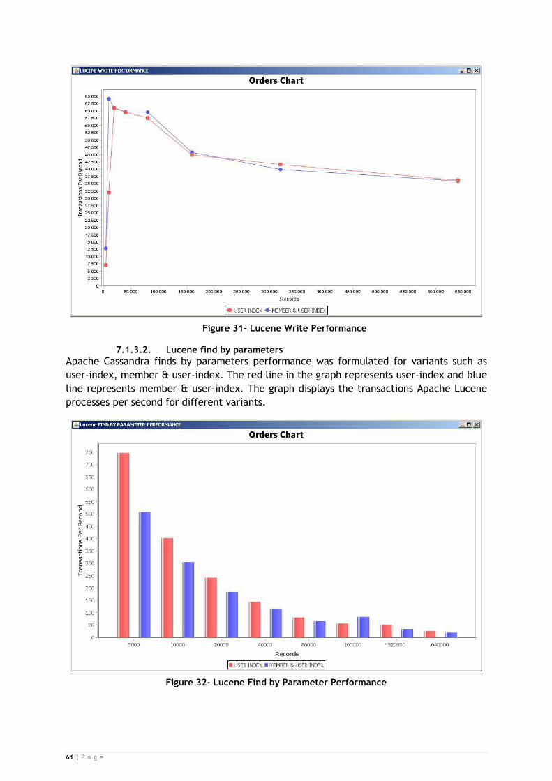
61 | P a g e
Figure 31- Lucene Write Performance
7.1.3.2. Lucene find by parameters
Apache Cassandra finds by parameters performance was formulated for variants such as
user-index, member & user-index. The red line in the graph represents user-index and blue
line represents member & user-index. The graph displays the transactions Apache Lucene
processes per second for different variants.
Figure 32- Lucene Find by Parameter Performance

62 | P a g e
Figure 33- Lucene Find by Parameter Performance
7.2. Performance Analysis MySQL and Lucene benchmarks were run on a development machine while Apache
Cassandra benchmarks were run on Virtual Machines (VMs) of 3-nodes cluster. VMS
introduced rough performance variation; due to many factors including network delays and
all the VMs sharing the same physical partition for the commit log. The intention was to
obtain the performance characteristics by running the benchmarks on VMs. Only
benchmarks run on dedicated physical machines can yield trustworthy results.
7.2.1. Write Performance
In case of write, MySQL processes 75-80 transactions per second, Apache Cassandra
processes 5,000 – 11,000 transactions per second, and Apache Lucene processes 30,000 –
60,000 transactions per second as shown in Figure 18- MySQL Write Performance, Figure
24- Cassandra Write Performance, and Figure 30- Lucene Write Performance
respectively.
Figure 19- MySQL Write Performance described that MySQL write performance almost
remains the same for different variants with different data size.
Cassandra write performance varies depending upon the variants as shown in Figure 25-
Cassandra Write Performance. It is quite evident that the write operation in Cassandra is
much faster if there is no index, but it becomes eventually slow, if we create indexes on
the columns. The number of transactions Cassandra processes for each variant remains the
same for the different data size.
Lucene write performance varies on the data size as shown in Figure 31- Lucene Write
Performance. Lucene started showing good performance. Index on one column performs
better than indexes on tuple. Inserting the huge amount of data makes the Lucene
performance again falls down.
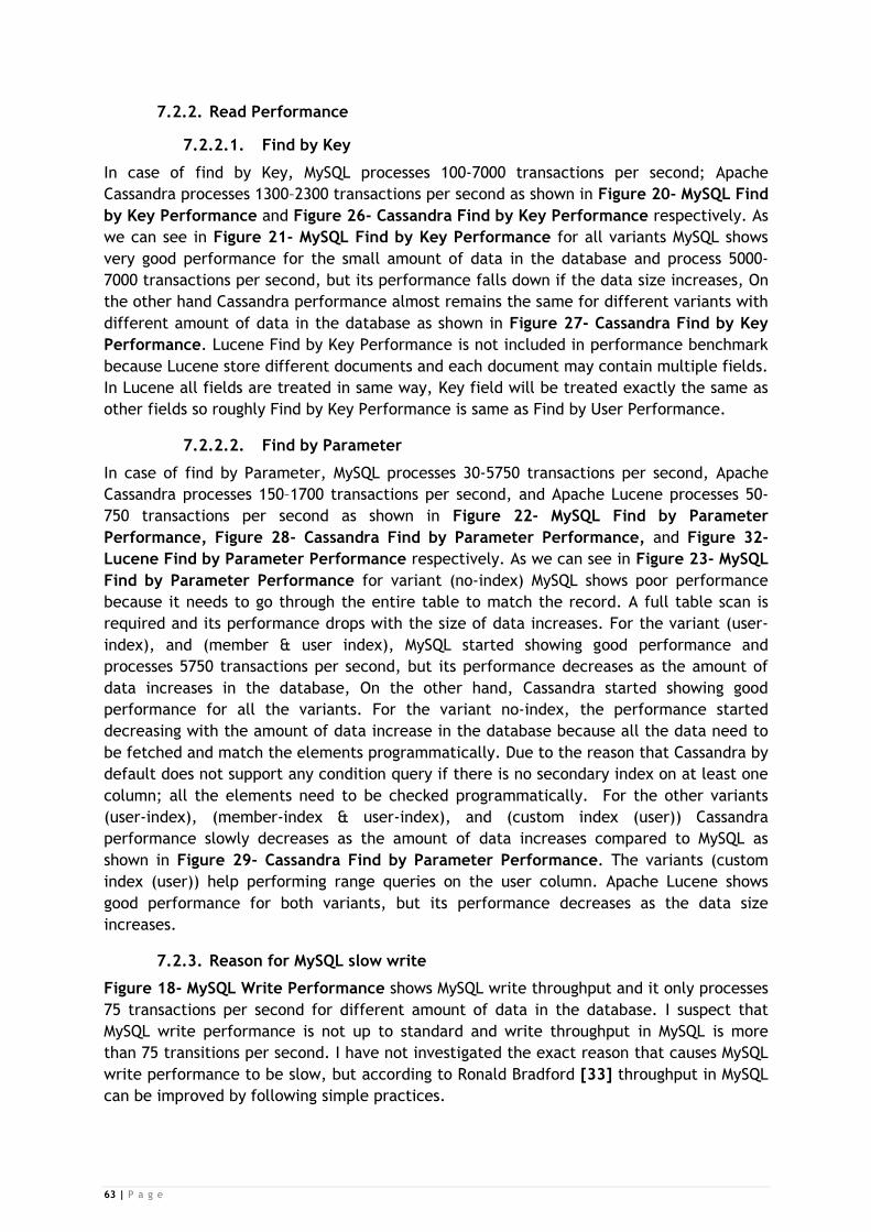
63 | P a g e
7.2.2. Read Performance
7.2.2.1. Find by Key
In case of find by Key, MySQL processes 100-7000 transactions per second; Apache
Cassandra processes 1300–2300 transactions per second as shown in Figure 20- MySQL Find
by Key Performance and Figure 26- Cassandra Find by Key Performance respectively. As
we can see in Figure 21- MySQL Find by Key Performance for all variants MySQL shows
very good performance for the small amount of data in the database and process 5000-
7000 transactions per second, but its performance falls down if the data size increases, On
the other hand Cassandra performance almost remains the same for different variants with
different amount of data in the database as shown in Figure 27- Cassandra Find by Key
Performance. Lucene Find by Key Performance is not included in performance benchmark
because Lucene store different documents and each document may contain multiple fields.
In Lucene all fields are treated in same way, Key field will be treated exactly the same as
other fields so roughly Find by Key Performance is same as Find by User Performance.
7.2.2.2. Find by Parameter
In case of find by Parameter, MySQL processes 30-5750 transactions per second, Apache
Cassandra processes 150–1700 transactions per second, and Apache Lucene processes 50-
750 transactions per second as shown in Figure 22- MySQL Find by Parameter
Performance, Figure 28- Cassandra Find by Parameter Performance, and Figure 32-
Lucene Find by Parameter Performance respectively. As we can see in Figure 23- MySQL
Find by Parameter Performance for variant (no-index) MySQL shows poor performance
because it needs to go through the entire table to match the record. A full table scan is
required and its performance drops with the size of data increases. For the variant (user-
index), and (member & user index), MySQL started showing good performance and
processes 5750 transactions per second, but its performance decreases as the amount of
data increases in the database, On the other hand, Cassandra started showing good
performance for all the variants. For the variant no-index, the performance started
decreasing with the amount of data increase in the database because all the data need to
be fetched and match the elements programmatically. Due to the reason that Cassandra by
default does not support any condition query if there is no secondary index on at least one
column; all the elements need to be checked programmatically. For the other variants
(user-index), (member-index & user-index), and (custom index (user)) Cassandra
performance slowly decreases as the amount of data increases compared to MySQL as
shown in Figure 29- Cassandra Find by Parameter Performance. The variants (custom
index (user)) help performing range queries on the user column. Apache Lucene shows
good performance for both variants, but its performance decreases as the data size
increases.
7.2.3. Reason for MySQL slow write
Figure 18- MySQL Write Performance shows MySQL write throughput and it only processes
75 transactions per second for different amount of data in the database. I suspect that
MySQL write performance is not up to standard and write throughput in MySQL is more
than 75 transitions per second. I have not investigated the exact reason that causes MySQL
write performance to be slow, but according to Ronald Bradford [33] throughput in MySQL
can be improved by following simple practices.
64 | P a g e
MySQL multi value capability shows 88 % improvement in performance [33]. Multi value
capability means multiple rows can be inserted using a single INSERT statement. Multiple
rows can be inserted using single statement as shown below
INSERT INTO table1 (col1, col2, col3) VALUES (?, ?, ?), (?, ?, ?);
Data can also be inserted using multiple INSERT statements as shown below.
INSERT INTO table1 (col1, col2, col3) VALUES (?, ?, ?);
INSERT INTO table1 (col1, col2, col3) VALUES (?, ?, ?);
INSERT INTO table1 (col1, col2, col3) VALUES (?, ?, ?);
Multiple INSERT statements work fine but its performance is not as efficient as single INSERT statement due to the overhead of back and forth of each SQL statement call. According to Ronland Bradford Max_allowed_packet is the system variable which can be
tuned for large INSERT statements.
In performance benchmark data is inserted using multiple INSERT statements. Little
modification in the code such as, insert data using single INSERT statement and adjust
Max_allowed_packet can increase write throughput significantly in MySQL.
7.2.4. Reason for Cassandra slow read
Cassandra is a write-oriented system, but still read performance can be enhanced by
tuning couple of parameters described in Improve read performance. In our performance
benchmark, there can be number of other factors also involved which can cause read
operation to become slow.
One obvious reason is reading from only single thread. It makes the read slow because of
distributed database architecture. Distributed database architecture is designed to serve
concurrent reads.
Secondly, we are not getting the advantage of Row Cache/Key Cache, because it takes
time to update the Key Cache/Row Cache after the data are inserted. In our case, we are
doing benchmarking for different data size having different variants, so that it drops the
databases, inserts new data and reads it quickly. During this time, no Row Cache/Key
Cache updates take place.
65 | P a g e
Chapter 8
8. Conclusion
The overall purpose of this research work was to investigate whether any database exists
which can handle historical financial data efficiently. In this regard, a research on
different architectures that exist today was conducted, so as to find efficient architecture
which has the ability to handle such data in an efficient manner. To find such architecture
and its performance for different variants, a performance benchmark was developed for
Apache Cassandra, Apache Lucene, and MySQL.
The thesis concludes that different databases exist, which can be of great help for
developers in order to handle large-scale information. However, to achieve this, the
developer must be willing to compromise some of the key features of traditional RDBMS
such as ACID. In this research work, Apache Cassandra was selected as a candidate keeping
Apache Lucene and MySQL as a reference. Apache Lucene and Apache Cassandra are
efficient solutions for storing and processing huge volumes of data. Apache Lucene runs on
the single machine and it is not horizontally scalable which makes it limited to handle
number of request. According to my point of view, these factors make Apache Cassandra a
stronger candidate for storing historical financial data in an efficient manner. Cinnober
Financial Technology AB currently uses Apache Lucene for storing and processing the data
for the History Server (HS). There are factors involved in which Apache Cassandra can be
considered. These are higher read and write throughput, larger amount of data in the
database, and a high number of client requests.
Cassandra benchmark model provides valuable information about Cassandra read and write
performance. Cassandra performance benchmark model was built for different variants
(no-index, user-index, member-index & user-index, and own-index (user)) to calculate
read and write throughput.
It was found that Apache Cassandra is an efficient solution for storing and processing the
huge amounts of data with different variants. Its performance remains the same even if
the size of data increases in the database. According to Abhinav Gopisetty [34] it is found
that Cassandra is horizontally scalable and both read and write throughput increase
linearly as new machines are added. Higher performance can also be achieved on a single
machine by performance tuning. Replication among the nodes in a cluster and built-in load
balancer are two powerful functionalities of Cassandra. Its architecture is best suited for
server which requires performing multiple read/write requests at same time and that has
been designed to handle large amounts of data distributed across the nodes in a cluster.
New node can easily be added in the cluster. Cassandra compromises the consistency and
it is considered as eventually consistent. Strong consistency can also be achieved in
Cassandra by specifying consistency level while reading or writing data. Consistency is not
always required and it depends upon the application. However, in case of Cinnober
Financial Technology AB, consistency was not the point of concern to improve the History
Server (HS).
66 | P a g e
8.1. Future work The performance benchmark I have built has limitations. Performance benchmark is
designed to handle one client request at a time. Cassandra is a distributed architecture
that is designed to handle multiple read/write requests at a time. Cassandra shows good
performance for multiple read/write requests. In case of write, it shows good performance
even for a single write request. But it was realized that Cassandra read throughput
performance was not up to the standard because of few reason described in Reason for
Cassandra slow read also MySQL write throughput performance was suspicious due to the
reasons described in Reason for MySQL slow write
In addition, I tried to make the performance benchmark more realistic by inserting random
data and based on assumptions created secondary indexes on frequent access fields. This
benchmark can be improved by obtaining real data and finding out the frequent access
fields by looking at logs. Inserting the real data and creating indexes based on logs will
definitely improve benchmark quality.
Future work can be aimed to address the above limitations such as in case of MySQL, write
data using single INSERT statement instead of using multiple INSERT statements and in case
of Cassandra, tune the concurrent reads. Moreover, design a more realistic performance
benchmark not only by inserting random data, but also by obtaining the real data. New
performance benchmark can be designed to improve performance, quality, and throughput
by handling these limitations.

67 | P a g e
References
1. NOSQL. http://en.citizendium.org/wiki/NoSQL. Accessed on March 18, 2012.
2. NOSQL Database Selection. http://blog.monitis.com/index.php/2011/05/22/picking-the-right-nosql-database-tool/. Accessed on June 2, 2012.
3. ACID Model. http://databases.about.com/od/specificproducts/a/acid.htm/ Accessed on June 1, 2012.
4. NOSQL Database Comparison. http://kkovacs.eu/cassandra-vs-mongodb-vs-couchdb-vs-redis. Accessed on March 28, 2012.
5. Apache Lucene Introduction. http://lucene.apache.org/core/. Accessed on April 20, 2012.
6. Apche Lucene. http://www.ibm.com/developerworks/library/wa-lucene/. Accessed on April 20, 2012.
7. NOSQL Benchmarking. http://www.cubrid.org/blog/dev-platform/nosql-benchmarking/. Accessed on March 30, 2012.
8. RDBMS. http://www.tutorialspoint.com/sql/sql-rdbms-concepts.htm. Accessed on March 30, 2012.
9. RDBMS VS NOSQL. http://blog.dynatrace.com/2011/10/05/nosql-or-rdbms-are-we-asking-the-right-questions/. Accessed on March 31, 2012.
10. Distributed Databases. http://it.toolbox.com/blogs/enterprise-solutions/overview-of-distributed-databases-16228. Accessed on April 20, 2012.
11. Apache Cassandra. http://kellabyte.com/2012/02/13/getting-started-using-apache-cassandra/. Accessed on April 20, 2012.
12. Apache Cassandra Partition. http://www.datastax.com/docs/1.0/cluster_architecture/partitioning. Accessed on May 10, 2012.
13. Apache Cassandra Replication. http://www.datastax.com/docs/0.8/cluster_architecture/replication. Accessed on May 10, 2012.
14. Apache Cassandra Request. http://www.datastax.com/docs/1.0/cluster_architecture/about_client_requests. Accessed on May 10, 2012.
15. Apache Cassandra Architecture. http://wiki.apache.org/cassandra/ArchitectureOverview. Accessed on May 10, 2012.
16. Apache Cassandra Clustering. http://www.datastax.com/docs/1.0/cluster_architecture/cluster_planning. Accessed on May 10, 2012.
17. Apache Cassandra Client. http://wiki.apache.org/cassandra/ClientOptions. Accessed on May 12, 2012.
18. Java. http://www.java.com/en/download/faq/whatis_java.xml. Accessed on May 17, 2012.
19. AB. http://www.ab.com. Accessed on June 10, 2012.
20. Apache Cassandra Indexes. http://www.datastax.com/docs/0.8/ddl/indexes. Accessed on June 26, 2012.
21. Brewer's Conjecture and the Feasibility of Consistent, Available, Partition-Tolerant Web Services. http://citeseerx.ist.psu.edu/viewdoc/download?doi=10.1.1.20.1495&rep=rep1&type=pdf.
22. Introduction to Cassandra. http://thelastpickle.com/files/2011-02-07-introduction-to-cassandra/introduction-to-cassandra.pdf.
23. Cassandra Documentation: Apache Cassandra 1.0 Documentation, DataStax, 2012.
24. T.Rabl, M.Sadoghi, H.Jacobsen, S.Gomez-Villamor, V.Muntes-Mulero and S.Mankovskii. Solving Big Data Challenges for Enterprise Application Performance Management, Proc. VLDB Endowment Vol.5, 2012.

68 | P a g e
25. J.Bohman, J.Hilding. “Cassandra”. Royal Institute of Technology, 2010.
26. NOSQL Databases. http://oak.cs.ucla.edu/cs144/handouts/nosqldbs.pdf.
27. R. Prasad Padhy, M.Ranjan Patra, S.Chandra Satapathy. RDBMS to NOSQL: Reviewing Some Next-Generation Non-Relational Database’s, Proc. IJAEST Vol.11, 2011.
28. G. DeCandia, D. Hastorun, M. Jampano, G.Kakulapati, A. Lakshman, A.Pilchin, S.Sivasubramanian, P.Vosshall, W.Vogels. Dynamo: Amazon’s Highly Avaialble Key-value Store, SOSP’07. ACM Press, Washington, USA.
29. Arto Salminen: Introduction to NOSQL. http://www.cs.tut.fi/~tjm/seminars/nosql2012/NoSQL-Intro.pdf, 2012.
30. F. Chang, J. Dean, S. Ghemawat, Wilson C. Hsieh, Deborah A. Wallach, M. Burrows, T. Chandra, A. Fikes, Robert E. Gruber. Bigtable: A Distributed Storage System for Structured Data, Proc. OSDI, 2006.
31. I.T. Varley. “No Relation: The Mixed Blessings of Non-Relational Databases”. The University of Texas at Austin, 2009.
32. NOSQL Scalability. http://www.w3resource.com/mongodb/nosql.php. Accessed on October 10, 2012.
33. Increase MySQL write throughput. http://ronaldbradford.com/blog/improving-mysql-insert-thoughput-2010-11-05/. Accessed on October 28, 2012.
34. Abhinav Gopisetty: A Survery on Cassandra and its performance with RDBMS and HBase.

69 | P a g e