Embed Size (px)
Citation preview

EUROPEAN ECONOMY
Economic and Financial Affairs
ISSN 2443-8049 (online)
1st Quarter 2017
TECHNICAL PAPER 015 | APRIL 2017
European BusinessCycle Indicators
EUROPEAN ECONOMY
European Economy Technical Papers are reports and data compiled by the staff of the European Commissionrsquos Directorate-General for Economic and Financial Affairs Authorised for publication by Joseacute Eduardo Leandro Director for Policy Strategy and Communication
LEGAL NOTICE Neither the European Commission nor any person acting on its behalf may be held responsible for the use which may be made of the information contained in this publication or for any errors which despite careful preparation and checking may appear This document exists in English only and can be downloaded from httpseceuropaeuinfopublicationseconomic-and-financial-affairs-publications_en It appears quarterly
Europe Direct is a service to help you find answers to your questions about the European Union
Freephone number () 00 800 6 7 8 9 10 11
() The information given is free as are most calls (though some operators phone boxes or hotels may charge you)
More information on the European Union is available on httpeuropaeu Luxembourg Publications Office of the European Union 2017
KC-BF-17-015-EN-N (online) KC-BF-17-015-EN-C (print) ISBN 978-92-79-64782-6 (online) ISBN 978-92-79-64781-9 (print) doi10276546681 (online) doi102765460709 (print)
copy European Union 2017 Reproduction is authorised provided the source is acknowledged Data whose source is not the European Union as identified in tables and charts of this publication is property of the named third party and therefore authorisation for its reproduction must be sought directly with the source
European Commission Directorate-General for Economic and Financial Affairs
European Business Cycle Indicators 1st Quarter 2017
Special topic Nowcasting the direction of euro-area GDP growth
This document is written by the staff of the Directorate-General for Economic and Financial Affairs Directorate A for Policy Strategy and Communication Unit A3 ndash Economic Situation Forecasts Business and Consumer Surveys httpeceuropaeuinfobusiness-economy-euroindicators-statisticseconomic-databasesbusiness-and-consumer-surveys_en Contact ChristianGayereceuropaeu EUROPEAN ECONOMY Technical Paper 015
CONTENTS
OVERVIEW 6
1 RECENT DEVELOPMENTS IN SURVEY INDICATORS 7
11 EU and euro area 7
12 Selected Member States 13
2 SPECIAL TOPIC NOWCASTING THE DIRECTION OF EURO-AREA GDP GROWTH 18
ANNEX 25
6
OVERVIEW
Recent developments in survey indicators
After having booked marked increases over the last quarter of 2016 the euro-area
and EU Economic Sentiment Indicators (ESI) remained broadly stable over the first
quarter of 2017 At 1079 (euro-area) and 1091 (EU) points both indicators remain
comfortably above their long-term averages of 100 at levels which were last
witnessed more than five (euro-area) or nine (EU) years ago
Also at the sectoral level developments were quite contained euro-area confidence
brightened in the construction and industry sectors and clouded over somewhat in
the retail trade sector The same holds for the EU whereby the improvement in
construction confidence was more forceful and the deterioration in retail trade
confidence much more contained
From a country perspective developments compared to December were rather
limited too Sentiment improved in the UK (+17) Poland (+16) Italy (+14) the
Netherlands (+11) and Spain (+09) while it cooled slightly in France (-06) and
Germany (-02)
Capacity utilisation in manufacturing increased by 02 percentage points in the euro
area and 03 percentage points in the EU Currently both indicators are about 1 frac12
percentage points above their respective long-term averages Capacity utilisation in
services remained unchanged in both the euro area and the EU also about 1 frac12
percentage points above their respective long-term averages
Special topic Nowcasting the direction of euro-area GDP growth
While a vast amount of econometric models have been developed to forecast Gross
Domestic Product (GDP) prior to its release the commonality of virtually all models is their
focus on predicting the growth rate of GDP Although obviously a highly relevant
estimation target we argue that correctly predicting the profile of GDP growth (ie whether
growth rates in- or decrease compared to the preceding quarter) can at times be even more
important from an economic or policy point of view In principle the expected growth
profile can simply be derived from a models forecasts of GDP growth However experience
shows that models producing high-quality point forecasts do not necessarily provide
particularly reliable information on the growth profile
Against that backdrop this special topic presents a number of new models explicitly tailored
to forecast the profile of GDP growth The models have in common that they rely to a large
extent on interaction terms ie variables measuring the effect of two developments
happening at the same time In a pseudo out-of-sample exercise the new models are shown
to provide rather reliable forecasts of the GDP profile resulting in hit ratios of 97 to 86
superior to the performance of the alternative approach of deriving the GDP profile from the
point forecasts of conventional bridge models predicting GDP growth
7
1 RECENT DEVELOPMENTS IN SURVEY INDICATORS
11 EU and euro area
Following sharp increases in the final quarter of
2016 the euro-area and EU Economic
Sentiment Indicators (ESI) stabilised at a high
level during the first quarter of 2017 Currently
standing at 1079 (euro-area) and 1091 (EU)
points respectively both indicators are not only
comfortably above their long-term averages of
100 but also at levels which were last
witnessed more than five (euro-area) or nine
(EU) years ago (see Graph 111)
Graph 111 Economic Sentiment Indicator
60
70
80
90
100
110
120
-6
-4
-2
0
2
4
6Euro area
60
70
80
90
100
110
120
-6
-4
-2
0
2
4
6
2009 2011 2013 2015 2017
EU
Real GDP growth (y-o-y) Economic Sent iment (rhs)
Note The horizontal line (rhs) marks the long-term average of the survey indicators Confidence indicators are expressed in balances
of opinion and hard data in y-o-y changes If necessary monthly
frequency is obtained by linear interpolation of quarterly data
While the ESI remained broadly unchanged in
the first quarter Markit Economics Composite
PMI for the euro area booked the strongest
increase in the course of a quarter since the
beginning of 2015 At 564 points the March-
reading is the highest in more than 5 frac12 years
Also the Ifo Business Climate Index (for
Germany) rose in the course of Q1 The
indicator currently stands at 1123 points its
highest level in more than 5 frac12 years
Graph 112 Radar Charts
Note A development away from the centre reflects an
improvement of a given indicator The ESI is computed with the
following sector weights industry 40 services 30 consumers 20 construction 5 retail trade 5 Series are normalised to a
mean of 100 and a standard deviation of 10 Historical averages
are generally calculated from 1990q1 For more information on the radar charts see the Special Topic in the 2016q1 EBCI
(httpseceuropaeuinfopublicationseconomy-
financeeuropean-business-cycle-indicators-1st-quarter-2016_en)
From a sectoral perspective confidence in the first
quarter of the year increased slightly among euro-
area managers in industry and construction (see
Graph 112) On the other hand confidence in the
retail trade sector cooled down somewhat while
consumer and services confidence stayed broadly
unchanged In the EU confidence improved
markedly in the construction sector and to a
much lesser degree in industry and among
consumers while it deteriorated slightly in the
services and retail trade sectors
In terms of levels almost all sectoral euro-area
and EU confidence indicators continue to be
significantly above their historical means only
8
services confidence in both regions has still not
lifted significantly above its long-term average
From a country perspective economic
sentiment improved mildly in five of the seven
largest EU economies namely in the UK
(+17) Poland (+16) Italy (+14) the
Netherlands (+11) and Spain (+09) while it
cooled slightly in France (-06) and Germany
(-02)
Sector developments
Industrial confidence in both the euro area and
the EU brightened slightly completing the first
quarter 12 points (euro area) and 11 points
(EU) higher than the preceding one As
illustrated by Graph 113 industry confidence
is rather high by historic standards at levels last
seen in mid-2011
Graph 113 Industry Confidence indicator
-50
-40
-30
-20
-10
0
10
20
-25
-15
-5
5
15Euro area
-50
-40
-30
-20
-10
0
10
20
-25
-15
-5
5
15
2009 2011 2013 2015 2017
EU
y-o-y industrial production growth
Industrial Confidence (rhs)
In both European aggregates the slight upward
trend of the confidence indicator resulted from
improvements in managers assessments of
order books while their assessments of the
stocks of finished products remained broadly
unchanged Regarding production expectations
managers were slightly more optimistic in the
euro area while in the EU production
expectations remained virtually stable
Of the components not included in the
confidence indicator past production in the
euro area deviated from the common trend
settling below its December level while export
order books appraisals were significantly more
upbeat than in December in both the euro area
and the EU
Euro-area and EU selling price expectations
continued the forceful recovery they had
embarked upon at the beginning of 2016
settling at their highest since mid-2011 The
same goes for employment expectations which
in March were as positive as last time in
summer 2011 (see Graph 114)
Graph 114 Employment - Industry Confidence
indicator
-50
-40
-30
-20
-10
0
10
-15
-10
-5
0
5Euro area
-50
-40
-30
-20
-10
0
10
-15
-10
-5
0
5
2009 2011 2013 2015 2017
EU
Employees manufacturing - growth
Employment expectations - Industry (rhs)
Focussing on the seven largest EU economies a
comparison of December and March readings
shows sharply improved industry confidence in
the UK (+56) and to a lesser extent Italy
(+29) Spain (+17) Germany (+14) and the
Netherlands (+13) Confidence in Poland
(+06) and France (-05) showed little change on
the quarter
The latest results of the quarterly manufacturing
survey (January) showed capacity utilisation
in manufacturing having increased by 02
percentage points in the euro area and 03
percentage points in the EU Currently both
indicators are about 1 frac12 percentage point above
their respective long-term averages (at 825 in
the euro area and 821 in the EU)
In line with the ESI trend euro-area services
confidence remained broadly unchanged (-02)
9
while it slightly deteriorated (-11) in the EU
Still both indicators score above their long-
term averages (see Graph 115)
Graph 115 Services Confidence indicator
-35
-25
-15
- 5
5
15
25
-8
-6
-4
-2
0
2
4
6Euro area
-35
-25
-15
- 5
5
15
25
-8
-6
-4
-2
0
2
4
6
2009 2011 2013 2015 2017
EU
Services value added growth Service Confidence (rhs)
Looking at the components of services
confidence assessments of the past business
situation and demand expectations worsened
while assessments of the past demand remained
broadly unchanged (EU) or improved (euro
area)
Compared to the end of Q4 employment
expectations in March remained virtually
unchanged both in the euro area and the EU
(see Graph 116) Selling price expectations
firmed in the euro area while they stayed
broadly unchanged in the EU
The flat signals from the services sector were
echoed in France (+03) Confidence brightened
in the Netherlands (+33) Italy (+18) and
Poland (+15) while it clouded over in the UK
(-51) Germany (-24) and Spain (-16)
Capacity utilisation in services as measured
by the January wave of the dedicated quarterly
survey remained unchanged in the euro area
and the EU The current rates of 894 (euro
area) and 893 (EU) correspond to levels
above the respective long-term averages
(calculated from 2011 onwards) of 878 and
881
Graph 116 Employment - Services Confidence
indicator
-20
-10
0
10
20
-4
-2
0
2
4Euro area
-20
-10
0
10
20
-4
-2
0
2
4
2009 2011 2013 2015 2017
EU
Employees services - growth
Employment expectations - Service (rhs)
Compared to the end of Q4 retail trade
confidence in March decreased somewhat in the
euro area (-17) and to a lesser extent in the EU
(-07) Both indicators stand comfortably above
their long-term averages (see Graph 117)
Graph 117 Retail Trade Confidence indicator
-30
-20
-10
0
10
-4
-3
-2
-1
0
1
2
3Euro area
-30
-20
-10
0
10
-4
-3
-2
-1
0
1
2
3
2009 2011 2013 2015 2017
EU
Consumption growth Retail Confidence (rhs)
A look at the individual components making up
the confidence indicator reveals that they
followed opposing trajectories while views on
the past business activity clouded over
assessments of the volume of stocks marginally
brightened Finally business expectations
10
slightly deteriorated in the euro area while they
mildly improved in the EU
Turning to a country perspective the months
since December saw retail trade confidence
improving in the UK (+37) Italy (+29) and
Poland (+17) while worsening in Germany
(-38) Spain (-20) France (-15) and more
mildly so in the Netherlands (-08)
Construction confidence continued the
recovery it had embarked upon in 2013 While
EU managers were much more upbeat (+42
points on the quarter) the improvements in the
euro area were somewhat more cautious (+22)
Graph 118 Construction Confidence indicator
-50
-40
-30
-20
-10
0
10
-15
-10
-5
0
5
10Euro area
-50
-40
-30
-20
-10
0
10
-15
-10
-5
0
5
10
2009 2011 2013 2015 2017
EU
Construction production growth
Construction Confidence (rhs)
In terms of the components making up the
indicator both EU and euro-area managers
reported much more positive appraisals of their
current order books while employment
expectations slightly improved in the EU and
remained virtually unchanged in the euro area
Focussing on the seven largest EU economies
construction confidence increased strongly in
the UK (+155) but also in the Netherlands
(+64) France (+31) Spain (+24) and Poland
(+15) Increases were more contained in
Germany (+09) and Italy (+04)
Consumer confidence remained broadly stable
during the first quarter Indicators increased by
01 points in the euro area and 04 points in the
EU scoring comfortably above their long-term
averages (see Graph 119)
While consumers expectations were much more
benign concerning unemployment and slightly
more optimistic concerning their savings they
were more pessimistic about their personal
financial situation and the general economic
situation
Graph 119 Consumer Confidence indicator
-40
-30
-20
-10
0
-4
-2
0
2
4Euro area
-40
-30
-20
-10
0
-4
-2
0
2
4
2009 2011 2013 2015 2017
EU
Consumption growth Consumer Confidence (rhs)
In terms of developments in the seven largest
EU economies the broadly flat developments
were echoed in Spain (+05) France (+04) and
the UK (+03) Confidence powered ahead in
the Netherlands (+34) and to some extent
Poland (+18) and Germany (+09) while it
deteriorated in Italy (-34)
EU and euro-area confidence in financial
services (not included in the ESI) booked solid
increases at the beginning of the year
completing the first quarter 98 (EU) to 117
(euro area) points higher than the previous one
The indicators are currently scoring at their
highest levels since 2011 (see Graph 1110)
In both regions appraisals of the past (demand
and business situation) contributed mostly to
the gains while the improvements in
expectations were somewhat more muted
11
Graph 1110 Financial Services Confidence indicator
-30
-10
10
30
-30
-10
10
30
Euro area
-30
-10
10
30
-30
-10
10
30
2009 2011 2013 2015 2017
EU
Financial Services Confidence
The positive developments in euro-areaEU
survey data over the fourth quarter are
illustrated by the evolution of the climate
tracers (see Annex for details)
Graph 1111 Euro area Climate Tracer
-4
-3
-2
-1
0
1
2
-04 -02 0 02
downswing
upswingcontraction
expansion
m-o-m change
lev
el
Mar-17
Jan-00
Jan-08
The economic climate tracers for the euro area
and the EU are comfortably settled in the
expansion area even slightly firmer than in
December 2016 (see Graphs 1111 and 1112)
The sectoral climate tracers (see Graph 1113)
are in line with the overall tracers in so far as all
of them indicate economic expansion as in
December Furthermore the services sector
indicators which were still close to the frontier
to the downswing area confirmed their position
in the expansion area
Graph 1112 EU Climate Tracer
-4
-3
-2
-1
0
1
2
-04 -02 0 02
downswing
upswingcontraction
expansion
m-o-m change
lev
el
Mar-17
Jan-00
Jan-08
12
Graph 1113 Economic climate tracers across sectors
Euro area EU
-4
-3
-2
-1
0
1
2
-05 -03 -01 01 03
Industry
downswing
upswingcontraction
expansion
m-o-m change
lev
el
Mar-17
Jan-00
Jan-08
-4
-3
-2
-1
0
1
2
-05 -03 -01 01 03
Industry
downswing
upswingcontraction
expansion
m-o-m change
lev
el
Mar-17
Jan-00
Jan-08
-3
-2
-1
0
1
2
-03 -01 01
Services
downswing
upswingcontraction
expansion
m-o-m change
lev
el
Mar-17
Jan-00
Jan-08
-3
-2
-1
0
1
2
-03 -01 01
Services
downswing
upswingcontraction
expansion
m-o-m change
lev
el
Mar-17
Jan-00
Jan-08
-4
-3
-2
-1
0
1
2
-05 -03 -01 01 03
Retail trade
downswing
upswingcontraction
expansion
m-o-m change
lev
el
Mar-17
Jan-00
Jan-08
-4
-3
-2
-1
0
1
2
-05 -03 -01 01 03
Retail trade
downswing
upswingcontraction
expansion
m-o-m change
lev
el
Mar-17
Jan-00
Jan-08
-3
-2
-1
0
1
2
-04 -02 0 02
Construction
downswing
upswingcontraction
expansion
m-o-m change
lev
el
Mar-17
Jan-00
Jan-08
-3
-2
-1
0
1
2
-04 -02 0 02
Construction
downswing
upswingcontraction
expansion
m-o-m change
lev
el
Mar-17
Jan-00
Jan-08
-3
-2
-1
0
1
2
-03 -01 01
Consumers
downswing
upswingcontraction
expansion
m-o-m change
lev
el
Mar-17
Jan-00
Jan-08
-3
-2
-1
0
1
2
-03 -01 01
Consumers
downswing
upswingcontraction
expansion
m-o-m change
lev
el
Mar-17
Jan-00
Jan-08
13
12 Selected Member States
Over the first quarter of 2017 changes in
sentiment were rather contained The
differences between the national indicators at
the end of 2016 and 2017 Q1 were positive in
the UK (+17) Poland (+16) Italy (+14) the
Netherlands (+11) and Spain (+09) and mildly
negative in Germany (-02) and France (-06)
In Germany a mild setback in economic
sentiment over the first two months of 2017 was
broadly offset by a commensurate increase in
March resulting in a broadly stable ESI in Q1
At 1092 points the indicator remained well
above its long-term average of 100 In terms of
the climate tracer (see Graph 121) the German
economy confirmed its position in the
expansion quadrant
Graph 121 Economic Sentiment Indicator
and Climate Tracer for Germany
60
70
80
90
100
110
120
-8
-6
-4
-2
0
2
4
6
2009 2011 2013 2015 2017
y-o-y real GDP growth (lhs) Economic Sent iment (rhs)
-3
-2
-1
0
1
2
-04 -02 0 02
downswing
upswingcontraction
expansion
m-o-m change
lev
el
Mar-17
Jan-00
Jan-08
From a sectoral perspective the first quarter
brought small improvements in industry and
among consumers while confidence clouded
over in the services and retail trade sectors
Confidence in the construction sector remained
virtually unchanged While all indicators
remained well above their respective long-term
averages (see Graph 122) the construction
sector is clearly enjoying an exceptionally high
confidence
Graph 122 Radar Chart for Germany
Note Given the high level of construction confidence the scale of the German radar chart extends to 130 unlike the other radar
charts in this publication
In France deteriorating sentiment in January
and March was mitigated by better readings in
February resulting in a mild cooling of
sentiment in Q1 At 1049 points the headline
indicator posts well above its long-term average
of 100 Accordingly the French climate tracer
(see Graph 123) is firmly settled in the
expansion quadrant
Graph 123 Economic Sentiment Indicator
and Climate Tracer for France
60
70
80
90
100
110
120
-6
-4
-2
0
2
4
2009 2011 2013 2015 2017
y-o-y real GDP growth (lhs) Economic Sent iment (rhs)
-3
-2
-1
0
1
2
-04 -02 0 02
downswing
upswingcontraction
expansion
m-o-m change
lev
el
Mar-17
Feb-03
Jan-08
14
A look at the French radar chart (see Graph
124) shows that only the construction sector
sent mildly positive signals while confidence
deteriorated in the retail trade sector In all other
sectors (industry services and consumers)
sentiment remained virtually unchanged In
terms of levels sentiment remained
comfortably above its long-term average in
industry and services and by a markedly
greater margin in retail trade and among
consumers In spite of its positive trend
construction confidence remained just below its
long-term average
Graph 124 Radar Chart for France
Due to an improvement in January followed by
virtually stable sentiment in February and
March the ESI in Italy settled above its level at
the end of 2016 (+14) At 1055 points the
Italian ESI confirmed its position firmly above
the long-term average of 100 As Graph 125
shows mildly improved sentiment in Q1 carried
the Italian climate tracer into the expansion
area coming from the frontier with the
downswing quadrant
Graph 125 Economic Sentiment Indicator
and Climate Tracer for Italy
60
70
80
90
100
110
120
-8
-6
-4
-2
0
2
4
2009 2011 2013 2015 2017
y-o-y real GDP growth (lhs) Economic Sent iment (rhs)
-3
-2
-1
0
1
2
3
-04 -02 0 02
downswing
upswingcontraction
expansion
m-o-m change
lev
el
Mar-17
Jan-00
Jan-08
Looking at the evolution of sectoral confidence
levels (see Graph 126) confidence brightened
in industry and to a lesser extent in retail trade
and services while it clouded over among
consumers and remained broadly stable in the
construction sector As in Q4 all sectoral
confidence indicators remained above their
long-term averages and most notably so the
indicator in retail trade
Graph 126 Radar Chart for Italy
15
While sentiment in Spain gained momentum at
the beginning of Q1 with increases in January
and February the last month of the quarter
brought a small set-back leaving the ESI just
09 points higher on the quarter At 1069
points the indicator increased its distance to the
long-term average of 100 The climate tracer for
Spain stayed virtually unchanged continuing to
locate the economy in the expansion quadrant
(see Graph 127)
Graph 127 Economic Sentiment Indicator
and Climate Tracer for Spain
60
70
80
90
100
110
120
-6
-4
-2
0
2
4
6
2009 2011 2013 2015 2017
y-o-y real GDP growth (lhs) Economic Sent iment (rhs)
-3
-2
-1
0
1
2
-04 -02 0 02
downswing
upswingcontraction
expansion
m-o-m change
lev
el
Mar-17
Jan-00
Jan-08
As the radar chart highlights (see Graph 128)
only the industry sector posted noteworthy
improvements in confidence while sentiment in
the retail trade sector deteriorated Nonetheless
same as in Q4 all sectoral confidence indicators
stayed well in excess of their respective long-
term averages with the notable exception of
construction which remained at historically low
levels
Graph 128 Radar Chart for Spain
Following positive developments in January
the Dutch sentiment reached a plateau at the
end of the first quarter At 1082 points the ESI
finished 11 points higher on the quarter and
remained well in excess of its long-term
average of 100 Propelled by the improvement
in sentiment the Dutch climate tracer (see
Graph 129) moved further into the expansion
area over Q1
Graph 129 Economic Sentiment Indicator
and Climate Tracer for the Netherlands
60
70
80
90
100
110
120
-6
-4
-2
0
2
4
6
2009 2011 2013 2015 2017
y-o-y real GDP growth (lhs) Economic Sent iment (rhs)
-3
-2
-1
0
1
2
-04 -02 0 02
downswing
upswingcontraction
expansion
m-o-m change
lev
el
Mar-17
Jan-00
Jan-08
A glance at the Dutch radar chart (see Graph
1210) shows that confidence improved in four
sectors (industry construction services and
consumers) and remained broadly unchanged
in the retail trade sector Compared to historic
16
levels confidence is high particularly among
consumers and in construction and rather low
in retail trade
Graph 1210 Radar Chart for the Netherlands
Sentiment in the United Kingdom continued
the rally it had embarked upon after the initial
shock of the Brexit referendum March data
came in 17 points higher on the quarter and
above their pre-referendum peak of June 2016
At 1102 points the UK ESI is firmly above its
long-term average of 100 The brighter
sentiment moved the UK climate tracer (see
Graph 1211) further into the expansion
quadrant
Graph 1211 Economic Sentiment Indicator
and Climate Tracer for the United Kingdom
50
70
90
110
130
-8
-6
-4
-2
0
2
4
6
2009 2011 2013 2015 2017
y-o-y real GDP growth (lhs) Economic Sent iment (rhs)
-4
-3
-2
-1
0
1
2
-04 -02 0 02
downswing
upswingcontraction
expansion
m-o-m change
lev
el
Mar-17
Jan-00
Jan-08
Focussing on sectoral developments the radar
chart for the UK (see Graph 1212) shows that
confidence increased markedly in construction
and industry and to a lesser extent in retail
trade while it cooled down in services and
remained broadly unchanged among consumers
The levels of confidence indexes are well in
excess of historic averages among consumers
and in retail trade and by a markedly greater
margin in industry and construction In the
services sector the decrease between December
and March brought the confidence indicator
back to its long-term average
Graph 1212 Radar Chart for the UK
Thanks mostly to a strong improvement in
January sentiment in Poland finished Q1 16
points above its Q4 level At 1027 the
indicator stayed above its long-term average
during the whole quarter for the first time since
2011 and reached its highest level since 2008
The improvement in sentiment moved the
climate tracer for Poland further into the
expansion quadrant (see Graph 1213)
17
Graph 1213 Economic Sentiment Indicator
and Climate Tracer for Poland
60
80
100
120
-1
1
3
5
7
2009 2011 2013 2015 2017
y-o-y real GDP growth (lhs) Economic Sent iment (rhs)
-3
-2
-1
0
1
2
3
-04 -02 0 02
downswing
upswingcontraction
expansion
m-o-m change
lev
el
Mar-17
Feb-03
Jan-08
As the Polish radar chart (see Graph 1214)
shows confidence has firmed across all sectors
of the economy All indicators remained above
their long-term averages with the exception of
the services sector which in spite of its positive
trend remained below but close to its long-term
average
Graph 1214 Radar Chart for Poland
18
2 SPECIAL TOPIC NOWCASTING THE DIRECTION OF EURO-AREA
GDP GROWTH
Introduction
Economic and political decision-makers base
their choices on an early understanding of the
state of the economy With the most
comprehensive measure of economic activity
Gross Domestic Product (GDP) released with
a significant time-lag1 a vast amount of
econometric models have been developed to
forecast GDP figures prior to their actual
release While there is abundant variety in
terms of the econometric techniques applied
and predictor variables deployed the
commonality of virtually all models is their
focus on predicting the growth rate of GDP
Although obviously a highly relevant
estimation target we argue that correctly
predicting the profile of GDP growth (ie
whether growth rates in- or decrease compared
to the preceding quarter) can at times be even
more important from an economicpolicy point
of view especially at turning points eg when
GDP starts picking up after a recession
In principle the expected growth profile can
simply be derived from a models forecasts of
GDP growth However experience shows that
models producing high-quality point forecasts
(in terms of root mean squared errors
(RMSEs)) do not necessarily provide
particularly reliable information on the growth
profile
Against that backdrop the present article
presents models which explicitly forecast the
profile of GDP growth Besides targeting a
dummy variable (taking the value one if GDP
growth is higher than in the preceding quarter)
the models differ from the current standard
models in respect of the selection of predictor
1 Eurostat publishes a first preliminary flash estimate of EA GDP
some 30 days after the reference quarter
variables relying to a significant extent on
interaction terms which are shown to be
particularly useful in the context of the
exercise
Our analysis constitutes to the best of the
authors knowledge the first attempt to
explicitly forecast the quarterly growth profile
of euro-area (EA) GDP growth and thus
complements a 2011-note by the French
Statistical Institute (Insee)2 which documents the
merits of such binary models for the case of
French GDP
The need for directional change
models
The pertinence of developing models explicitly
tailored to forecasting the profile of GDP
growth can be illustrated by looking at the
reliability of information which other existing
models provide in respect of the GDP growth
profile Concretely one can simply derive the
GDP profile from the forecasts of standard
bridge models targeting quarter-on-quarter (q-
o-q) GDP growth To test the merits of that
approach we rely on four short-term models
regularly operated by DG ECFIN whose
performance in forecasting EA GDP growth is
at par with other well-reputed models like
Bank of Italys euro-coin indicator3 and which
cover a variety of different econometric
approaches and types of predictor variables
Two of them are standard bridge models based
on survey indicators (BM1 and BM2) The
2 Mikol F and M Cornec (2011) Will activity accelerate or slow
down A few tools to answer the question French National Institute of Statistics and Economic Studies Conjoncture in
France December 3 The RMSEs of DG ECFINs bridge models and the euro-coin
indicator produced at the end of the reference quarter cluster
around 025 (percentage-points of q-o-q GDP growth) over the period 2010q1 to 2016q4
19
time-varying parameter model (TVP) is also
based on survey data but differs from the
former in that parameters are allowed to
change over time The last one (FM) is a factor
model4 As another benchmark a naiumlve
autoregressive model is also run Finally the
pooling approach (POOL) is based on the
average of the nowcasts of the above models
Table 21 summarises the forecasting
performance of the different models as
generated by a pseudo real-time exercise
covering the period 2010q1 to 2016q4 (ie 28
quarters) and assuming that forecasts are
conducted at the end of the third month of each
quarter ie 30 days before the first estimate of
GDP (preliminary flash) is released5 As it
turns out even the best performing models do
not achieve to correctly identify the GDP
growth profile6 in more than 20 out of 28
cases which translates into a rate of 717
Table 21 Nowcasting performance by model (2010q1-
2016q4) correct in-decreases (out of 28)
BM1 TVP BM2 FM AR POOL
20 18 19 19 20 20
Particularities of the target variable
Before turning to the presentation of the new
(directional change) models some thoughts on
the target variable are warranted Generally to
assess the performance of models nowcasting
the (continuous) GDP growth rate it is
considered sufficient and valid to work in
pseudo real-time ie with the last revised
vintage of GDP (see Diron 20068) This is due
4
For more details about the factor model see Gayer C A
Girardi and A Reuter (2014) The role of survey data in
nowcasting euro area GDP growth European Commission
European Economy Economic Papers 538 5 Note that the preliminary flash only exists since 2016q2 Prior to
that date the first release of GDP (flash estimate) got
available 45 days after the end of the reference quarter 6 The GDP growth profile is derived from the real-time flash
estimates as explained below 7 That percentage is statistically significantly different from the
predictions of a random guess model (equivalent to repeatedly tossing a coin) at the 99 significance level
8 Diron M (2006) Short-term forecasts of euro area real GDP
growth an assessment of real-time performance based on
to the fact that revisions of the target variable
(GDP growth) are usually rather contained
Unfortunately that does not necessarily hold
true when forecasting the profile of GDP
since even small revisions in GDP growth can
lead to changes in the GDP profile
Against that backdrop one has to make a
conscious choice in respect of the version of
GDP whose growth profile one wants to
nowcast We argue that most users of GDP
nowcasts (analysts policy makers etc) tend to
judge their reliability by comparing them to
timely releases of GDP rather than revised
figures getting available several months later
Accordingly we choose to construct our target
variable on the basis of the flash estimates of
GDP which get released some 45 days after
the reference quarter9 In line with our
theoretical considerations the binary variable
derived from real-time data is quite different
from the one based on the last revised GDP
series available on the Eurostat website from
2001q1 to 2013q4 the growth profiles
signalled by the two variables differ in 31 of
cases
The dataset
In order to explicitly nowcast the quarterly
growth profile of EA GDP our target variable
is a binary (dummy) series Its value is defined
as one whenever the real-time q-o-q GDP
growth is higher than in the previous quarter
and zero otherwise
In terms of potential predictor variables to
choose from we consider a wide array of time-
series typically deployed in the context of
GDP forecasting ranging from business and
consumer surveys (BCS) to hard data such as
industrial production (IP) etc Since we focus
on the development of models forecasting the
GDP profile at the end of the third month of a
quarter (where a number of variables relating
to the forecasting quarter have not yet been
vintage data European Central Bank ECB working paper
series No 622 May 9 The data are retrieved from the Revisions Analysis Dataset
provided by the OECD which is available here httpstatsoecdorgindexaspxqueryid=206
20
released) some variables (eg IP) are only
partially included in the dataset
All variables considered in our analysis are in
a first step subject to the typical
transformations ensuring their stationarity (eg
trending variables such as IP are expressed as
growth rates) Given that our dependent
variable is based on the difference of the
usually targeted GDP growth rate we also
express each transformed variable (i) in terms
of first differences and (ii) as a dummy
variable indicating whether that difference is
positive We thus end up with three versions of
each variable being included in the data-set
Apart from the standard variables mentioned
above our data-set also includes a new
variable called correction term which is the
difference between the fitted values of a
survey (BCS)-based regression targeting GDP
growth and the actual realisation of GDP
growth Given the close statistical relationship
between GDP growth and the survey data
(BCS) whenever the term is positive (ie GDP
growth is lower than suggested by surveys) it
signals an increased likelihood that GDP
growth in the next quarter will accelerate (and
vice versa)10
The models
Intermediate models
Following the approach developed by Insee
our first attempt to model the GDP growth
profile involves the estimation of a logit model
using only survey variables as predictors
While the resulting model performs quite well
on French data the approach turns out to be
rather ineffective at EA level presumably
because EA GDP growth is much smoother
As a consequence the approach is broadened
so as to allow the inclusion of other types of
variables (hard and financial data) Although
variables typically considered in GDP models
10 The exact regression underlying the indicator-construction is
growth(GDP)t = ESIt + ΔESIt As a robustness check the indicator has also been derived from other survey variables
than the Economic Sentiment Indicator (ESI) The resulting
variables generally displayed a high degree of comovement with the initial correction term
are included (IP retail sales etc) the
performance of the models is rather
unsatisfactory with the best logit model
achieving a correct identification of ac-
decelerations of output in just 77 of cases11
The results can be rationalised when
considering that the individual ability of the
input variables to correctly signal ac-
decelerations of GDP growth is less
pronounced than the co-movement of their
trend-cycle component with that of GDP
growth which is exploited in the usual models
targeting GDP growth After all even a
variable like IP in the manufacturing sector
whose merits for the forecast of GDP growth
are well-documented moves only in 68 of
the quarters in the same direction as GDP
growth12
Final models
Given the limited qualification of the available
input variables for the purpose of forecasting
the GDP profile the new models presented in
this section follow a novel strategy which is to
focus mainly on interactions of variables
rather than a number of isolated predictors
The approach is motivated by the
consideration that for GDP not just to grow
but to grow faster than in the previous quarter
a particular constellation or momentum is
required Our assumption is that a decisive
difference between episodes of growth and of
accelerating growth is that in the latter certain
positive developments happen at the same
time Put differently the joint effect of certain
developments occurring simultaneously is
supposed to be higher than the sum of the
effects of the two developments occurring in
isolation Econometrically the joint effect is
captured by interaction terms ie series which
11 The detailed results are not reported due to space constraints
but can be shared upon request 12 This percentage was computed over the period 2010q1-2016q4
with IP values restricted to the first month of the reference
quarter (as is realistic in the light of the significant time-lag
of IP releases) Every quarterly value corresponds to the IP q-o-q growth resulting from the level of IP in month 1 of the
reference quarter (assumed to stay constant over months 2
and 3) compared to the average level of IP in the previous quarter
21
represent the product of two independent
variables
Besides allowing a better measurement of
momentum the use of interaction terms also
helps to render certain variables with a mixed
effect on GDP growth more meaningful
Rising inflation for instance might be a proxy
of rallying demand (associated with strong
GDP growth) but also of rising input prices
(eg oil) associated with weaker demand and
GDP growth While the effect of inflation
might thus not be significant in a regression
targeting GDP growth the interaction of
inflation and oil prices could well be (notably
negative)
The selection of models presented in Table 22
is the result of a bottom-up testing approach in
which variables were incrementally added to
the model13
and their marginal effect on the
proportion of explained variance of the target
variable (R-squared) monitored The range of
possible input variables was determined based
on variables correlation with the target
variable (ie the GDP profile) and whether
their inclusion in the model made sense from
an economic point of view
13 The models are estimated with standard ordinary least squares
(OLS) since they contain one or several dummy explanatory
variables Furthermore the estimation of the variance has
been rendered heteroskedasticity-robust (using Newey-West estimators)
Table 22
coeff
Model 1 (2001q2 - 2016q3) - R2 062
constant 056
ESI-based correction term t-1 101
dummy (Δ industry selling price expectations t-1 gt 0) 006 Δ industry past orders development t
Δ services past business situation t 007 Δ -change money supply M2 t-1
construction confidence t-1 002 dummy (Δ industry confidence t-1 gt 0)
dummy (Δ PMI construction t gt 0) 006 Δ construction employment expectations t-1
Model 2 (2001q2 - 2016q3) - R2 058
constant 032
dummy (-change money supply M1 t gt 0) 023
Δ -change manufacturing production t 020 dummy (Δ -change raw material price index t lt 0)
dummy (Δ -change raw material price index t gt 0) 083 Δ Ifo world economic climate t
dummy (Δ consumers expected major purchases t gt 0) 012 Δ presence of above-average stocks in retail sector t
Model 3 (2001q2 - 2016q3) - R2 063
constant 034
dummy (-change money supply M1 t gt 0) 020
ESI-based correction term t-1 043
Δ -change manufacturing production t 018 dummy (Δ -change raw material price index t lt 0)
dummy (Δ -change raw material price index t gt 0) 073 Δ Ifo world economic climate t
dummy (Δ consumers expected major purchases t gt 0) 012 Δ presence of above-average stocks in retail sector t
Model 4 (2001q2 - 2016q3) - R2 066
constant 040
ESI-based correction term t-1 106
dummy (Δ -change retail sales t-1 gt0) 010 Δ PMI Composite t
-change exports of goods out of EA t-1 005 dummy (Δ -change commodity price index excl energy t
gt0)
Δ -change production of machinery and equipment t 008 dummy (Δ -change commodity price index t-1 gt 0)
Δ consumers savings expectations t 0005 consumers expected major purchases t
Note Three asterisks indicate significance at the 1-level two
asterisks at the 5-level
22
While it would go beyond the scope of this
article to discuss every model in detail a
number of commonalities among them can be
pointed out (i) Three of the models include the
Economic Sentiment Indicator (ESI)-based
correction term highlighting its ability to
signal increases in GDP growth rates (ii) All
models include at least one variable from the
industry sector which is in line with the well-
documented impact of IP on the variation of
GDP growth Furthermore the role of retail
trade and consumer sentiment seems to be
prominent with elements of both featuring in
three of the models That contrasts with the
services and construction sectors which are
only included in Model 1 (iii) There are four
types of interaction terms which all seem
helpful to capture momentum for GDP
growth to increase
first interactions which combine
developments in different sectors of
the economy such as the penultimate
variable of Model 1 which considers
the level of construction confidence
when it coincides with an increase in
industry confidence The justification
for that type of interaction is that it
captures whether a given tendency in
the economy (here buoyant
confidence in construction) is an
isolated trend or a phenomenon
observed across different sectors of the
economy When the latter applies the
chances for an acceleration in GDP
growth are arguably significantly
enhanced
second interactions which relate
sector-specific developments to
variables impacting on the entire
economy such as the third variable of
Model 2 which captures changes in
manufacturing production growth only
when they coincide with a deceleration
of raw material prices The rationale of
such interactions is that positive
developments in a given economic
sector are more likely to result in an
acceleration of GDP growth when
they happen in a growth-friendly
overall context (eg an environment of
low input prices low interest rates
etc)
third interactions which capture the
simultaneous occurrence of certain
external developments with a
potentially stimulating effect on the
economy under investigation The
penultimate variable of Model 2 is an
example of that category considering
changes in world economic climate
whenever growth in raw material
prices is accelerating Taking account
of changes in the price levels of raw
materials helps distilling particularly
pronounced and sustained upswings in
world demand rather than
temporaryshort ones
fourth there are interactions which
render variables with a potentially
mixed effect on GDP growth
meaningful For instance the last
variable of Model 3 considers changes
in retail trade stocks only when they
occur in conjunction with higher
expected demand The interaction thus
filters out situations in which retail
trade stocks pile up because of a lack
of demand and retains only incidents
where stocks are accumulated in the
expectation of higher demand
Having established a good in-sample fit of the
four models we test their performance in a
(pseudo) out-of sample exercise over a period
stretching from the financial crisis to the
current edge (2008q2 to 2016q4)14
The
predictions of the models are interpreted as
signalling accelerations whenever they attach a
probability larger 05 to an increase in GDP
growth The opposite applies to decelerations
Figures 21 to 24 summarise the results
As the graphs show all four models perform
very well at predicting output ac-
decelerations in almost all cases in which the
difference in GDP growth (black line) is in
positive territory the blue bars (which
14 The starting point for the out-of sample exercise could not be
chosen earlier since the models can only be run from
2001q12001q2 onwards (due to limited data availability)
and some 20 quarters of in-sample observations were deemed necessary to estimate meaningful coefficients
23
represent the forecasts expressed as deviations
from 05) are positive too The opposite holds
true when the GDP line turns negative The
few incorrect predictions are highlighted as red
bars Depending on the model there are one
(Model 1) to five (Model 2) of them
Considering the length of the out-of sample
exercise (35 quarters) the models are thus
correct in 97 to 86 of cases which
represents a big improvement in precision
compared to deriving directional nowcasts
from the models presented in the above
sections
The forecasting performance appears even
more convincing when taking a closer look at
the wrong predictions (red bars) and the
associated actual changes in GDP growth
rates As regards the former in at least half of
the cases where the models fail this is because
they are forced to produce a clear-cut
judgment (increase or decrease of GDP
growth) although they actually cannot distil
any clear signal from the data at all (ie the
predicted values are close to 05) Against that
backdrop one might consider introducing a
blind zone for the interpretation of the
models predictions ie a range of predicted
probabilities which are so close to 05 that
forecasts falling into the interval are
interpreted as signalling neither an ac- nor a
deceleration of GDP growth A visual
inspection of the graphs suggests that the
interval from 042 to 058 might be an
appropriate blind zone allowing to increase
the percentage of correctly identified ac-
decelerations while at the same time
keeping the amount of quarters where the
models fail to deliver forecasts reasonably
limited Indeed when applying an 042-058
blind zone Model 1 gets flawless Model 3
produces a single while Models 24 just two
wrong predictions At the same time applying
the blind zone causes models to be unable to
produce nowcasts in just 2 (Model 4) to 5
(Model 3) quarters and thus less than 15 of
the observed period
Turning to the actual differences in GDP
growth rates observed in the quarters where
our models produce wrong forecasts several
of those differences are very marginal and
would probably be interpreted as signalling
stable output rather than ac- or decelerations
of economic activity When the models err in
those circumstances one might argue that the
mistake is less grave than usual since the
actual economic developments are not the
exact opposite of the models predictions As
evidenced by graphs 21 to 24 several of our
models errors can thus be relativized notably
wrong predictions in 2008q3 (by Model 3)
2011q3 (by Model 2) and 2016q4 (by Models
2 and 4)
Figure 21 Model 1
Figure 22 Model 2
Figure 23 Model 3
24
Figure 24 Model 4
Note The black lines represent the q-o-q differences in GDP
growth ie values above (below) 0 indicate accelerations (decelerations) of economic activity Since the cut-off for the
categorisation of the models predictions into accelerations and
decelerations of output is 05 the blue bars represent the predicted values minus 05
Conclusions
Departing from the observation that correctly
predicting the profile of GDP growth can at
times be more important from an
economicpolicy point of view than getting a
reasonable estimate of the actual growth rate
this special topic presents a number of new
models explicitly tailored to forecast the profile
of GDP growth The models have in common
that they rely to a large extent on interaction
terms ie variables measuring the effect of two
developments happening at the same time (eg
IP and retail sales rising simultaneously) It
appears that those interaction terms do a good
job capturing the momentum that is required
for GDP not just to grow but to grow faster
than in the preceding quarter
In a pseudo out-of-sample exercise the new
models are shown to provide rather reliable
forecasts of the GDP profile with the best
model producing just a single and the worst a
total of five wrong predictions over a sample of
35 quarters The resulting hit ratios of 97 to
86 are shown to be superior to the
performance of alternative approaches such as
the derivation of the GDP profile from the point
forecasts of conventional bridge models
predicting GDP growth
In addition to their merits for the forecast of in-
decreases in GDP growth the new models also
have the potential to enhance the quality of the
point forecasts of GDP growth generated by
conventional bridge models Concretely when
the latter indicate a growth rate whose error
bands include the level of the previous quarters
growth rate the forecasts from the new models
could justify considering some part of the error
bands irrelevant (namely the part which lies
between last quarters growth rate and the lower
(upper) end of the error band when the new
models predict an acceleration (deceleration) of
output) The combined reading of the two
approaches can thus help reduce the uncertainty
around the nowcasts
25
ANNEX
Reference series
Confidence
indicators
Reference series from Eurostat via Ecowin
(volumeyear-on-year growth rates)
Total economy (ESI) GDP seasonally- and calendar-adjusted
Industry Industrial production working day-adjusted
Services Gross value added for the private services sector seasonally- and calendar-adjusted
Consumption Household and NPISH final consumption expenditure seasonally- and calendar-adjusted
Retail Household and NPISH final consumption expenditure seasonally- and calendar-adjusted
Building Production index for building and civil engineering trend-cycle component
Economic Sentiment Indicator
The economic sentiment indicator (ESI) is a weighted average of the balances of replies to selected
questions addressed to firms and consumers in five sectors covered by the EU Business and
Consumer Surveys Programme The sectors covered are industry (weight 40 ) services (30 )
consumers (20 ) retail (5 ) and construction (5 )
Balances are constructed as the difference between the percentages of respondents giving positive and
negative replies EU and euro-area aggregates are calculated on the basis of the national results and
seasonally adjusted The ESI is scaled to a long-term mean of 100 and a standard deviation of 10
Thus values above 100 indicate above-average economic sentiment and vice versa Further details on
the construction of the ESI can be found here
Long time series (ESI and confidence indices) are available here
Economic Climate Tracer
The economic climate tracer is a two-stage procedure The first stage consists of building economic
climate indicators based on principal component analyses of balance series (sa) from five surveys
The input series are as follows industry five of the monthly survey questions (employment and
selling-price expectations are excluded) services all five monthly questions consumers nine
questions (price-related questions and the question about the current financial situation are excluded)
retail all five monthly questions building all four monthly questions The economic climate
indicator (ECI) is a weighted average of the five sector climate indicators The sector weights are
equal to those underlying the Economic Sentiment Indicator (ESI see above)
In the second stage all climate indicators are smoothed using the HP filter in order to eliminate short-
term fluctuations of a period of less than 18 months The smoothed series are then normalised (zero
mean and unit standard deviation) The resulting series are plotted against their first differences The
four quadrants of the graph corresponding to the four business cycle phases are crossed in an anti-
clockwise movement and can be described as above average and increasing (top right lsquoexpansionrsquo)
above average but decreasing (top left lsquodownswingrsquo) below average and decreasing (bottom left
lsquocontractionrsquo) and below average but increasing (bottom right lsquoupswingrsquo) Cyclical peaks are
positioned in the top centre of the graph and troughs in the bottom centre In order to make the graphs
more readable two colours have been used for the tracer The darker line shows developments in the
current cycle which in the EU and euro area roughly started in January 2008
EUROPEAN ECONOMY TECHNICAL PAPERS European Economy Technical Papers can be accessed and downloaded free of charge from the following address httpeceuropaeueconomy_financepublicationseetpindex_enhtm Titles published before July 2015 can be accessed and downloaded free of charge from httpeceuropaeueconomy_financepublicationscycle_indicatorsindex_enhtm (European Business Cycle Indicators)
Alternatively hard copies may be ordered via the ldquoPrint-on-demandrdquo service offered by the EU Bookshop httpbookshopeuropaeu
HOW TO OBTAIN EU PUBLICATIONS Free publications bull one copy
via EU Bookshop (httpbookshopeuropaeu) bull more than one copy or postersmaps
- from the European Unionrsquos representations (httpeceuropaeurepresent_enhtm) - from the delegations in non-EU countries (httpseeaseuropaeuheadquartersheadquarters-homepageareageo_en) - by contacting the Europe Direct service (httpeuropaeueuropedirectindex_enhtm) or calling 00 800 6 7 8 9 10 11 (freephone number from anywhere in the EU) () () The information given is free as are most calls (though some operators phone boxes or hotels may charge you)
Priced publications bull via EU Bookshop (httpbookshopeuropaeu)
ISBN 978-92-79-64782-6
KC-BF-17-015-EN-N

6
OVERVIEW
Recent developments in survey indicators
After having booked marked increases over the last quarter of 2016 the euro-area
and EU Economic Sentiment Indicators (ESI) remained broadly stable over the first
quarter of 2017 At 1079 (euro-area) and 1091 (EU) points both indicators remain
comfortably above their long-term averages of 100 at levels which were last
witnessed more than five (euro-area) or nine (EU) years ago
Also at the sectoral level developments were quite contained euro-area confidence
brightened in the construction and industry sectors and clouded over somewhat in
the retail trade sector The same holds for the EU whereby the improvement in
construction confidence was more forceful and the deterioration in retail trade
confidence much more contained
From a country perspective developments compared to December were rather
limited too Sentiment improved in the UK (+17) Poland (+16) Italy (+14) the
Netherlands (+11) and Spain (+09) while it cooled slightly in France (-06) and
Germany (-02)
Capacity utilisation in manufacturing increased by 02 percentage points in the euro
area and 03 percentage points in the EU Currently both indicators are about 1 frac12
percentage points above their respective long-term averages Capacity utilisation in
services remained unchanged in both the euro area and the EU also about 1 frac12
percentage points above their respective long-term averages
Special topic Nowcasting the direction of euro-area GDP growth
While a vast amount of econometric models have been developed to forecast Gross
Domestic Product (GDP) prior to its release the commonality of virtually all models is their
focus on predicting the growth rate of GDP Although obviously a highly relevant
estimation target we argue that correctly predicting the profile of GDP growth (ie whether
growth rates in- or decrease compared to the preceding quarter) can at times be even more
important from an economic or policy point of view In principle the expected growth
profile can simply be derived from a models forecasts of GDP growth However experience
shows that models producing high-quality point forecasts do not necessarily provide
particularly reliable information on the growth profile
Against that backdrop this special topic presents a number of new models explicitly tailored
to forecast the profile of GDP growth The models have in common that they rely to a large
extent on interaction terms ie variables measuring the effect of two developments
happening at the same time In a pseudo out-of-sample exercise the new models are shown
to provide rather reliable forecasts of the GDP profile resulting in hit ratios of 97 to 86
superior to the performance of the alternative approach of deriving the GDP profile from the
point forecasts of conventional bridge models predicting GDP growth
7
1 RECENT DEVELOPMENTS IN SURVEY INDICATORS
11 EU and euro area
Following sharp increases in the final quarter of
2016 the euro-area and EU Economic
Sentiment Indicators (ESI) stabilised at a high
level during the first quarter of 2017 Currently
standing at 1079 (euro-area) and 1091 (EU)
points respectively both indicators are not only
comfortably above their long-term averages of
100 but also at levels which were last
witnessed more than five (euro-area) or nine
(EU) years ago (see Graph 111)
Graph 111 Economic Sentiment Indicator
60
70
80
90
100
110
120
-6
-4
-2
0
2
4
6Euro area
60
70
80
90
100
110
120
-6
-4
-2
0
2
4
6
2009 2011 2013 2015 2017
EU
Real GDP growth (y-o-y) Economic Sent iment (rhs)
Note The horizontal line (rhs) marks the long-term average of the survey indicators Confidence indicators are expressed in balances
of opinion and hard data in y-o-y changes If necessary monthly
frequency is obtained by linear interpolation of quarterly data
While the ESI remained broadly unchanged in
the first quarter Markit Economics Composite
PMI for the euro area booked the strongest
increase in the course of a quarter since the
beginning of 2015 At 564 points the March-
reading is the highest in more than 5 frac12 years
Also the Ifo Business Climate Index (for
Germany) rose in the course of Q1 The
indicator currently stands at 1123 points its
highest level in more than 5 frac12 years
Graph 112 Radar Charts
Note A development away from the centre reflects an
improvement of a given indicator The ESI is computed with the
following sector weights industry 40 services 30 consumers 20 construction 5 retail trade 5 Series are normalised to a
mean of 100 and a standard deviation of 10 Historical averages
are generally calculated from 1990q1 For more information on the radar charts see the Special Topic in the 2016q1 EBCI
(httpseceuropaeuinfopublicationseconomy-
financeeuropean-business-cycle-indicators-1st-quarter-2016_en)
From a sectoral perspective confidence in the first
quarter of the year increased slightly among euro-
area managers in industry and construction (see
Graph 112) On the other hand confidence in the
retail trade sector cooled down somewhat while
consumer and services confidence stayed broadly
unchanged In the EU confidence improved
markedly in the construction sector and to a
much lesser degree in industry and among
consumers while it deteriorated slightly in the
services and retail trade sectors
In terms of levels almost all sectoral euro-area
and EU confidence indicators continue to be
significantly above their historical means only
8
services confidence in both regions has still not
lifted significantly above its long-term average
From a country perspective economic
sentiment improved mildly in five of the seven
largest EU economies namely in the UK
(+17) Poland (+16) Italy (+14) the
Netherlands (+11) and Spain (+09) while it
cooled slightly in France (-06) and Germany
(-02)
Sector developments
Industrial confidence in both the euro area and
the EU brightened slightly completing the first
quarter 12 points (euro area) and 11 points
(EU) higher than the preceding one As
illustrated by Graph 113 industry confidence
is rather high by historic standards at levels last
seen in mid-2011
Graph 113 Industry Confidence indicator
-50
-40
-30
-20
-10
0
10
20
-25
-15
-5
5
15Euro area
-50
-40
-30
-20
-10
0
10
20
-25
-15
-5
5
15
2009 2011 2013 2015 2017
EU
y-o-y industrial production growth
Industrial Confidence (rhs)
In both European aggregates the slight upward
trend of the confidence indicator resulted from
improvements in managers assessments of
order books while their assessments of the
stocks of finished products remained broadly
unchanged Regarding production expectations
managers were slightly more optimistic in the
euro area while in the EU production
expectations remained virtually stable
Of the components not included in the
confidence indicator past production in the
euro area deviated from the common trend
settling below its December level while export
order books appraisals were significantly more
upbeat than in December in both the euro area
and the EU
Euro-area and EU selling price expectations
continued the forceful recovery they had
embarked upon at the beginning of 2016
settling at their highest since mid-2011 The
same goes for employment expectations which
in March were as positive as last time in
summer 2011 (see Graph 114)
Graph 114 Employment - Industry Confidence
indicator
-50
-40
-30
-20
-10
0
10
-15
-10
-5
0
5Euro area
-50
-40
-30
-20
-10
0
10
-15
-10
-5
0
5
2009 2011 2013 2015 2017
EU
Employees manufacturing - growth
Employment expectations - Industry (rhs)
Focussing on the seven largest EU economies a
comparison of December and March readings
shows sharply improved industry confidence in
the UK (+56) and to a lesser extent Italy
(+29) Spain (+17) Germany (+14) and the
Netherlands (+13) Confidence in Poland
(+06) and France (-05) showed little change on
the quarter
The latest results of the quarterly manufacturing
survey (January) showed capacity utilisation
in manufacturing having increased by 02
percentage points in the euro area and 03
percentage points in the EU Currently both
indicators are about 1 frac12 percentage point above
their respective long-term averages (at 825 in
the euro area and 821 in the EU)
In line with the ESI trend euro-area services
confidence remained broadly unchanged (-02)
9
while it slightly deteriorated (-11) in the EU
Still both indicators score above their long-
term averages (see Graph 115)
Graph 115 Services Confidence indicator
-35
-25
-15
- 5
5
15
25
-8
-6
-4
-2
0
2
4
6Euro area
-35
-25
-15
- 5
5
15
25
-8
-6
-4
-2
0
2
4
6
2009 2011 2013 2015 2017
EU
Services value added growth Service Confidence (rhs)
Looking at the components of services
confidence assessments of the past business
situation and demand expectations worsened
while assessments of the past demand remained
broadly unchanged (EU) or improved (euro
area)
Compared to the end of Q4 employment
expectations in March remained virtually
unchanged both in the euro area and the EU
(see Graph 116) Selling price expectations
firmed in the euro area while they stayed
broadly unchanged in the EU
The flat signals from the services sector were
echoed in France (+03) Confidence brightened
in the Netherlands (+33) Italy (+18) and
Poland (+15) while it clouded over in the UK
(-51) Germany (-24) and Spain (-16)
Capacity utilisation in services as measured
by the January wave of the dedicated quarterly
survey remained unchanged in the euro area
and the EU The current rates of 894 (euro
area) and 893 (EU) correspond to levels
above the respective long-term averages
(calculated from 2011 onwards) of 878 and
881
Graph 116 Employment - Services Confidence
indicator
-20
-10
0
10
20
-4
-2
0
2
4Euro area
-20
-10
0
10
20
-4
-2
0
2
4
2009 2011 2013 2015 2017
EU
Employees services - growth
Employment expectations - Service (rhs)
Compared to the end of Q4 retail trade
confidence in March decreased somewhat in the
euro area (-17) and to a lesser extent in the EU
(-07) Both indicators stand comfortably above
their long-term averages (see Graph 117)
Graph 117 Retail Trade Confidence indicator
-30
-20
-10
0
10
-4
-3
-2
-1
0
1
2
3Euro area
-30
-20
-10
0
10
-4
-3
-2
-1
0
1
2
3
2009 2011 2013 2015 2017
EU
Consumption growth Retail Confidence (rhs)
A look at the individual components making up
the confidence indicator reveals that they
followed opposing trajectories while views on
the past business activity clouded over
assessments of the volume of stocks marginally
brightened Finally business expectations
10
slightly deteriorated in the euro area while they
mildly improved in the EU
Turning to a country perspective the months
since December saw retail trade confidence
improving in the UK (+37) Italy (+29) and
Poland (+17) while worsening in Germany
(-38) Spain (-20) France (-15) and more
mildly so in the Netherlands (-08)
Construction confidence continued the
recovery it had embarked upon in 2013 While
EU managers were much more upbeat (+42
points on the quarter) the improvements in the
euro area were somewhat more cautious (+22)
Graph 118 Construction Confidence indicator
-50
-40
-30
-20
-10
0
10
-15
-10
-5
0
5
10Euro area
-50
-40
-30
-20
-10
0
10
-15
-10
-5
0
5
10
2009 2011 2013 2015 2017
EU
Construction production growth
Construction Confidence (rhs)
In terms of the components making up the
indicator both EU and euro-area managers
reported much more positive appraisals of their
current order books while employment
expectations slightly improved in the EU and
remained virtually unchanged in the euro area
Focussing on the seven largest EU economies
construction confidence increased strongly in
the UK (+155) but also in the Netherlands
(+64) France (+31) Spain (+24) and Poland
(+15) Increases were more contained in
Germany (+09) and Italy (+04)
Consumer confidence remained broadly stable
during the first quarter Indicators increased by
01 points in the euro area and 04 points in the
EU scoring comfortably above their long-term
averages (see Graph 119)
While consumers expectations were much more
benign concerning unemployment and slightly
more optimistic concerning their savings they
were more pessimistic about their personal
financial situation and the general economic
situation
Graph 119 Consumer Confidence indicator
-40
-30
-20
-10
0
-4
-2
0
2
4Euro area
-40
-30
-20
-10
0
-4
-2
0
2
4
2009 2011 2013 2015 2017
EU
Consumption growth Consumer Confidence (rhs)
In terms of developments in the seven largest
EU economies the broadly flat developments
were echoed in Spain (+05) France (+04) and
the UK (+03) Confidence powered ahead in
the Netherlands (+34) and to some extent
Poland (+18) and Germany (+09) while it
deteriorated in Italy (-34)
EU and euro-area confidence in financial
services (not included in the ESI) booked solid
increases at the beginning of the year
completing the first quarter 98 (EU) to 117
(euro area) points higher than the previous one
The indicators are currently scoring at their
highest levels since 2011 (see Graph 1110)
In both regions appraisals of the past (demand
and business situation) contributed mostly to
the gains while the improvements in
expectations were somewhat more muted
11
Graph 1110 Financial Services Confidence indicator
-30
-10
10
30
-30
-10
10
30
Euro area
-30
-10
10
30
-30
-10
10
30
2009 2011 2013 2015 2017
EU
Financial Services Confidence
The positive developments in euro-areaEU
survey data over the fourth quarter are
illustrated by the evolution of the climate
tracers (see Annex for details)
Graph 1111 Euro area Climate Tracer
-4
-3
-2
-1
0
1
2
-04 -02 0 02
downswing
upswingcontraction
expansion
m-o-m change
lev
el
Mar-17
Jan-00
Jan-08
The economic climate tracers for the euro area
and the EU are comfortably settled in the
expansion area even slightly firmer than in
December 2016 (see Graphs 1111 and 1112)
The sectoral climate tracers (see Graph 1113)
are in line with the overall tracers in so far as all
of them indicate economic expansion as in
December Furthermore the services sector
indicators which were still close to the frontier
to the downswing area confirmed their position
in the expansion area
Graph 1112 EU Climate Tracer
-4
-3
-2
-1
0
1
2
-04 -02 0 02
downswing
upswingcontraction
expansion
m-o-m change
lev
el
Mar-17
Jan-00
Jan-08
12
Graph 1113 Economic climate tracers across sectors
Euro area EU
-4
-3
-2
-1
0
1
2
-05 -03 -01 01 03
Industry
downswing
upswingcontraction
expansion
m-o-m change
lev
el
Mar-17
Jan-00
Jan-08
-4
-3
-2
-1
0
1
2
-05 -03 -01 01 03
Industry
downswing
upswingcontraction
expansion
m-o-m change
lev
el
Mar-17
Jan-00
Jan-08
-3
-2
-1
0
1
2
-03 -01 01
Services
downswing
upswingcontraction
expansion
m-o-m change
lev
el
Mar-17
Jan-00
Jan-08
-3
-2
-1
0
1
2
-03 -01 01
Services
downswing
upswingcontraction
expansion
m-o-m change
lev
el
Mar-17
Jan-00
Jan-08
-4
-3
-2
-1
0
1
2
-05 -03 -01 01 03
Retail trade
downswing
upswingcontraction
expansion
m-o-m change
lev
el
Mar-17
Jan-00
Jan-08
-4
-3
-2
-1
0
1
2
-05 -03 -01 01 03
Retail trade
downswing
upswingcontraction
expansion
m-o-m change
lev
el
Mar-17
Jan-00
Jan-08
-3
-2
-1
0
1
2
-04 -02 0 02
Construction
downswing
upswingcontraction
expansion
m-o-m change
lev
el
Mar-17
Jan-00
Jan-08
-3
-2
-1
0
1
2
-04 -02 0 02
Construction
downswing
upswingcontraction
expansion
m-o-m change
lev
el
Mar-17
Jan-00
Jan-08
-3
-2
-1
0
1
2
-03 -01 01
Consumers
downswing
upswingcontraction
expansion
m-o-m change
lev
el
Mar-17
Jan-00
Jan-08
-3
-2
-1
0
1
2
-03 -01 01
Consumers
downswing
upswingcontraction
expansion
m-o-m change
lev
el
Mar-17
Jan-00
Jan-08
13
12 Selected Member States
Over the first quarter of 2017 changes in
sentiment were rather contained The
differences between the national indicators at
the end of 2016 and 2017 Q1 were positive in
the UK (+17) Poland (+16) Italy (+14) the
Netherlands (+11) and Spain (+09) and mildly
negative in Germany (-02) and France (-06)
In Germany a mild setback in economic
sentiment over the first two months of 2017 was
broadly offset by a commensurate increase in
March resulting in a broadly stable ESI in Q1
At 1092 points the indicator remained well
above its long-term average of 100 In terms of
the climate tracer (see Graph 121) the German
economy confirmed its position in the
expansion quadrant
Graph 121 Economic Sentiment Indicator
and Climate Tracer for Germany
60
70
80
90
100
110
120
-8
-6
-4
-2
0
2
4
6
2009 2011 2013 2015 2017
y-o-y real GDP growth (lhs) Economic Sent iment (rhs)
-3
-2
-1
0
1
2
-04 -02 0 02
downswing
upswingcontraction
expansion
m-o-m change
lev
el
Mar-17
Jan-00
Jan-08
From a sectoral perspective the first quarter
brought small improvements in industry and
among consumers while confidence clouded
over in the services and retail trade sectors
Confidence in the construction sector remained
virtually unchanged While all indicators
remained well above their respective long-term
averages (see Graph 122) the construction
sector is clearly enjoying an exceptionally high
confidence
Graph 122 Radar Chart for Germany
Note Given the high level of construction confidence the scale of the German radar chart extends to 130 unlike the other radar
charts in this publication
In France deteriorating sentiment in January
and March was mitigated by better readings in
February resulting in a mild cooling of
sentiment in Q1 At 1049 points the headline
indicator posts well above its long-term average
of 100 Accordingly the French climate tracer
(see Graph 123) is firmly settled in the
expansion quadrant
Graph 123 Economic Sentiment Indicator
and Climate Tracer for France
60
70
80
90
100
110
120
-6
-4
-2
0
2
4
2009 2011 2013 2015 2017
y-o-y real GDP growth (lhs) Economic Sent iment (rhs)
-3
-2
-1
0
1
2
-04 -02 0 02
downswing
upswingcontraction
expansion
m-o-m change
lev
el
Mar-17
Feb-03
Jan-08
14
A look at the French radar chart (see Graph
124) shows that only the construction sector
sent mildly positive signals while confidence
deteriorated in the retail trade sector In all other
sectors (industry services and consumers)
sentiment remained virtually unchanged In
terms of levels sentiment remained
comfortably above its long-term average in
industry and services and by a markedly
greater margin in retail trade and among
consumers In spite of its positive trend
construction confidence remained just below its
long-term average
Graph 124 Radar Chart for France
Due to an improvement in January followed by
virtually stable sentiment in February and
March the ESI in Italy settled above its level at
the end of 2016 (+14) At 1055 points the
Italian ESI confirmed its position firmly above
the long-term average of 100 As Graph 125
shows mildly improved sentiment in Q1 carried
the Italian climate tracer into the expansion
area coming from the frontier with the
downswing quadrant
Graph 125 Economic Sentiment Indicator
and Climate Tracer for Italy
60
70
80
90
100
110
120
-8
-6
-4
-2
0
2
4
2009 2011 2013 2015 2017
y-o-y real GDP growth (lhs) Economic Sent iment (rhs)
-3
-2
-1
0
1
2
3
-04 -02 0 02
downswing
upswingcontraction
expansion
m-o-m change
lev
el
Mar-17
Jan-00
Jan-08
Looking at the evolution of sectoral confidence
levels (see Graph 126) confidence brightened
in industry and to a lesser extent in retail trade
and services while it clouded over among
consumers and remained broadly stable in the
construction sector As in Q4 all sectoral
confidence indicators remained above their
long-term averages and most notably so the
indicator in retail trade
Graph 126 Radar Chart for Italy
15
While sentiment in Spain gained momentum at
the beginning of Q1 with increases in January
and February the last month of the quarter
brought a small set-back leaving the ESI just
09 points higher on the quarter At 1069
points the indicator increased its distance to the
long-term average of 100 The climate tracer for
Spain stayed virtually unchanged continuing to
locate the economy in the expansion quadrant
(see Graph 127)
Graph 127 Economic Sentiment Indicator
and Climate Tracer for Spain
60
70
80
90
100
110
120
-6
-4
-2
0
2
4
6
2009 2011 2013 2015 2017
y-o-y real GDP growth (lhs) Economic Sent iment (rhs)
-3
-2
-1
0
1
2
-04 -02 0 02
downswing
upswingcontraction
expansion
m-o-m change
lev
el
Mar-17
Jan-00
Jan-08
As the radar chart highlights (see Graph 128)
only the industry sector posted noteworthy
improvements in confidence while sentiment in
the retail trade sector deteriorated Nonetheless
same as in Q4 all sectoral confidence indicators
stayed well in excess of their respective long-
term averages with the notable exception of
construction which remained at historically low
levels
Graph 128 Radar Chart for Spain
Following positive developments in January
the Dutch sentiment reached a plateau at the
end of the first quarter At 1082 points the ESI
finished 11 points higher on the quarter and
remained well in excess of its long-term
average of 100 Propelled by the improvement
in sentiment the Dutch climate tracer (see
Graph 129) moved further into the expansion
area over Q1
Graph 129 Economic Sentiment Indicator
and Climate Tracer for the Netherlands
60
70
80
90
100
110
120
-6
-4
-2
0
2
4
6
2009 2011 2013 2015 2017
y-o-y real GDP growth (lhs) Economic Sent iment (rhs)
-3
-2
-1
0
1
2
-04 -02 0 02
downswing
upswingcontraction
expansion
m-o-m change
lev
el
Mar-17
Jan-00
Jan-08
A glance at the Dutch radar chart (see Graph
1210) shows that confidence improved in four
sectors (industry construction services and
consumers) and remained broadly unchanged
in the retail trade sector Compared to historic
16
levels confidence is high particularly among
consumers and in construction and rather low
in retail trade
Graph 1210 Radar Chart for the Netherlands
Sentiment in the United Kingdom continued
the rally it had embarked upon after the initial
shock of the Brexit referendum March data
came in 17 points higher on the quarter and
above their pre-referendum peak of June 2016
At 1102 points the UK ESI is firmly above its
long-term average of 100 The brighter
sentiment moved the UK climate tracer (see
Graph 1211) further into the expansion
quadrant
Graph 1211 Economic Sentiment Indicator
and Climate Tracer for the United Kingdom
50
70
90
110
130
-8
-6
-4
-2
0
2
4
6
2009 2011 2013 2015 2017
y-o-y real GDP growth (lhs) Economic Sent iment (rhs)
-4
-3
-2
-1
0
1
2
-04 -02 0 02
downswing
upswingcontraction
expansion
m-o-m change
lev
el
Mar-17
Jan-00
Jan-08
Focussing on sectoral developments the radar
chart for the UK (see Graph 1212) shows that
confidence increased markedly in construction
and industry and to a lesser extent in retail
trade while it cooled down in services and
remained broadly unchanged among consumers
The levels of confidence indexes are well in
excess of historic averages among consumers
and in retail trade and by a markedly greater
margin in industry and construction In the
services sector the decrease between December
and March brought the confidence indicator
back to its long-term average
Graph 1212 Radar Chart for the UK
Thanks mostly to a strong improvement in
January sentiment in Poland finished Q1 16
points above its Q4 level At 1027 the
indicator stayed above its long-term average
during the whole quarter for the first time since
2011 and reached its highest level since 2008
The improvement in sentiment moved the
climate tracer for Poland further into the
expansion quadrant (see Graph 1213)
17
Graph 1213 Economic Sentiment Indicator
and Climate Tracer for Poland
60
80
100
120
-1
1
3
5
7
2009 2011 2013 2015 2017
y-o-y real GDP growth (lhs) Economic Sent iment (rhs)
-3
-2
-1
0
1
2
3
-04 -02 0 02
downswing
upswingcontraction
expansion
m-o-m change
lev
el
Mar-17
Feb-03
Jan-08
As the Polish radar chart (see Graph 1214)
shows confidence has firmed across all sectors
of the economy All indicators remained above
their long-term averages with the exception of
the services sector which in spite of its positive
trend remained below but close to its long-term
average
Graph 1214 Radar Chart for Poland
18
2 SPECIAL TOPIC NOWCASTING THE DIRECTION OF EURO-AREA
GDP GROWTH
Introduction
Economic and political decision-makers base
their choices on an early understanding of the
state of the economy With the most
comprehensive measure of economic activity
Gross Domestic Product (GDP) released with
a significant time-lag1 a vast amount of
econometric models have been developed to
forecast GDP figures prior to their actual
release While there is abundant variety in
terms of the econometric techniques applied
and predictor variables deployed the
commonality of virtually all models is their
focus on predicting the growth rate of GDP
Although obviously a highly relevant
estimation target we argue that correctly
predicting the profile of GDP growth (ie
whether growth rates in- or decrease compared
to the preceding quarter) can at times be even
more important from an economicpolicy point
of view especially at turning points eg when
GDP starts picking up after a recession
In principle the expected growth profile can
simply be derived from a models forecasts of
GDP growth However experience shows that
models producing high-quality point forecasts
(in terms of root mean squared errors
(RMSEs)) do not necessarily provide
particularly reliable information on the growth
profile
Against that backdrop the present article
presents models which explicitly forecast the
profile of GDP growth Besides targeting a
dummy variable (taking the value one if GDP
growth is higher than in the preceding quarter)
the models differ from the current standard
models in respect of the selection of predictor
1 Eurostat publishes a first preliminary flash estimate of EA GDP
some 30 days after the reference quarter
variables relying to a significant extent on
interaction terms which are shown to be
particularly useful in the context of the
exercise
Our analysis constitutes to the best of the
authors knowledge the first attempt to
explicitly forecast the quarterly growth profile
of euro-area (EA) GDP growth and thus
complements a 2011-note by the French
Statistical Institute (Insee)2 which documents the
merits of such binary models for the case of
French GDP
The need for directional change
models
The pertinence of developing models explicitly
tailored to forecasting the profile of GDP
growth can be illustrated by looking at the
reliability of information which other existing
models provide in respect of the GDP growth
profile Concretely one can simply derive the
GDP profile from the forecasts of standard
bridge models targeting quarter-on-quarter (q-
o-q) GDP growth To test the merits of that
approach we rely on four short-term models
regularly operated by DG ECFIN whose
performance in forecasting EA GDP growth is
at par with other well-reputed models like
Bank of Italys euro-coin indicator3 and which
cover a variety of different econometric
approaches and types of predictor variables
Two of them are standard bridge models based
on survey indicators (BM1 and BM2) The
2 Mikol F and M Cornec (2011) Will activity accelerate or slow
down A few tools to answer the question French National Institute of Statistics and Economic Studies Conjoncture in
France December 3 The RMSEs of DG ECFINs bridge models and the euro-coin
indicator produced at the end of the reference quarter cluster
around 025 (percentage-points of q-o-q GDP growth) over the period 2010q1 to 2016q4
19
time-varying parameter model (TVP) is also
based on survey data but differs from the
former in that parameters are allowed to
change over time The last one (FM) is a factor
model4 As another benchmark a naiumlve
autoregressive model is also run Finally the
pooling approach (POOL) is based on the
average of the nowcasts of the above models
Table 21 summarises the forecasting
performance of the different models as
generated by a pseudo real-time exercise
covering the period 2010q1 to 2016q4 (ie 28
quarters) and assuming that forecasts are
conducted at the end of the third month of each
quarter ie 30 days before the first estimate of
GDP (preliminary flash) is released5 As it
turns out even the best performing models do
not achieve to correctly identify the GDP
growth profile6 in more than 20 out of 28
cases which translates into a rate of 717
Table 21 Nowcasting performance by model (2010q1-
2016q4) correct in-decreases (out of 28)
BM1 TVP BM2 FM AR POOL
20 18 19 19 20 20
Particularities of the target variable
Before turning to the presentation of the new
(directional change) models some thoughts on
the target variable are warranted Generally to
assess the performance of models nowcasting
the (continuous) GDP growth rate it is
considered sufficient and valid to work in
pseudo real-time ie with the last revised
vintage of GDP (see Diron 20068) This is due
4
For more details about the factor model see Gayer C A
Girardi and A Reuter (2014) The role of survey data in
nowcasting euro area GDP growth European Commission
European Economy Economic Papers 538 5 Note that the preliminary flash only exists since 2016q2 Prior to
that date the first release of GDP (flash estimate) got
available 45 days after the end of the reference quarter 6 The GDP growth profile is derived from the real-time flash
estimates as explained below 7 That percentage is statistically significantly different from the
predictions of a random guess model (equivalent to repeatedly tossing a coin) at the 99 significance level
8 Diron M (2006) Short-term forecasts of euro area real GDP
growth an assessment of real-time performance based on
to the fact that revisions of the target variable
(GDP growth) are usually rather contained
Unfortunately that does not necessarily hold
true when forecasting the profile of GDP
since even small revisions in GDP growth can
lead to changes in the GDP profile
Against that backdrop one has to make a
conscious choice in respect of the version of
GDP whose growth profile one wants to
nowcast We argue that most users of GDP
nowcasts (analysts policy makers etc) tend to
judge their reliability by comparing them to
timely releases of GDP rather than revised
figures getting available several months later
Accordingly we choose to construct our target
variable on the basis of the flash estimates of
GDP which get released some 45 days after
the reference quarter9 In line with our
theoretical considerations the binary variable
derived from real-time data is quite different
from the one based on the last revised GDP
series available on the Eurostat website from
2001q1 to 2013q4 the growth profiles
signalled by the two variables differ in 31 of
cases
The dataset
In order to explicitly nowcast the quarterly
growth profile of EA GDP our target variable
is a binary (dummy) series Its value is defined
as one whenever the real-time q-o-q GDP
growth is higher than in the previous quarter
and zero otherwise
In terms of potential predictor variables to
choose from we consider a wide array of time-
series typically deployed in the context of
GDP forecasting ranging from business and
consumer surveys (BCS) to hard data such as
industrial production (IP) etc Since we focus
on the development of models forecasting the
GDP profile at the end of the third month of a
quarter (where a number of variables relating
to the forecasting quarter have not yet been
vintage data European Central Bank ECB working paper
series No 622 May 9 The data are retrieved from the Revisions Analysis Dataset
provided by the OECD which is available here httpstatsoecdorgindexaspxqueryid=206
20
released) some variables (eg IP) are only
partially included in the dataset
All variables considered in our analysis are in
a first step subject to the typical
transformations ensuring their stationarity (eg
trending variables such as IP are expressed as
growth rates) Given that our dependent
variable is based on the difference of the
usually targeted GDP growth rate we also
express each transformed variable (i) in terms
of first differences and (ii) as a dummy
variable indicating whether that difference is
positive We thus end up with three versions of
each variable being included in the data-set
Apart from the standard variables mentioned
above our data-set also includes a new
variable called correction term which is the
difference between the fitted values of a
survey (BCS)-based regression targeting GDP
growth and the actual realisation of GDP
growth Given the close statistical relationship
between GDP growth and the survey data
(BCS) whenever the term is positive (ie GDP
growth is lower than suggested by surveys) it
signals an increased likelihood that GDP
growth in the next quarter will accelerate (and
vice versa)10
The models
Intermediate models
Following the approach developed by Insee
our first attempt to model the GDP growth
profile involves the estimation of a logit model
using only survey variables as predictors
While the resulting model performs quite well
on French data the approach turns out to be
rather ineffective at EA level presumably
because EA GDP growth is much smoother
As a consequence the approach is broadened
so as to allow the inclusion of other types of
variables (hard and financial data) Although
variables typically considered in GDP models
10 The exact regression underlying the indicator-construction is
growth(GDP)t = ESIt + ΔESIt As a robustness check the indicator has also been derived from other survey variables
than the Economic Sentiment Indicator (ESI) The resulting
variables generally displayed a high degree of comovement with the initial correction term
are included (IP retail sales etc) the
performance of the models is rather
unsatisfactory with the best logit model
achieving a correct identification of ac-
decelerations of output in just 77 of cases11
The results can be rationalised when
considering that the individual ability of the
input variables to correctly signal ac-
decelerations of GDP growth is less
pronounced than the co-movement of their
trend-cycle component with that of GDP
growth which is exploited in the usual models
targeting GDP growth After all even a
variable like IP in the manufacturing sector
whose merits for the forecast of GDP growth
are well-documented moves only in 68 of
the quarters in the same direction as GDP
growth12
Final models
Given the limited qualification of the available
input variables for the purpose of forecasting
the GDP profile the new models presented in
this section follow a novel strategy which is to
focus mainly on interactions of variables
rather than a number of isolated predictors
The approach is motivated by the
consideration that for GDP not just to grow
but to grow faster than in the previous quarter
a particular constellation or momentum is
required Our assumption is that a decisive
difference between episodes of growth and of
accelerating growth is that in the latter certain
positive developments happen at the same
time Put differently the joint effect of certain
developments occurring simultaneously is
supposed to be higher than the sum of the
effects of the two developments occurring in
isolation Econometrically the joint effect is
captured by interaction terms ie series which
11 The detailed results are not reported due to space constraints
but can be shared upon request 12 This percentage was computed over the period 2010q1-2016q4
with IP values restricted to the first month of the reference
quarter (as is realistic in the light of the significant time-lag
of IP releases) Every quarterly value corresponds to the IP q-o-q growth resulting from the level of IP in month 1 of the
reference quarter (assumed to stay constant over months 2
and 3) compared to the average level of IP in the previous quarter
21
represent the product of two independent
variables
Besides allowing a better measurement of
momentum the use of interaction terms also
helps to render certain variables with a mixed
effect on GDP growth more meaningful
Rising inflation for instance might be a proxy
of rallying demand (associated with strong
GDP growth) but also of rising input prices
(eg oil) associated with weaker demand and
GDP growth While the effect of inflation
might thus not be significant in a regression
targeting GDP growth the interaction of
inflation and oil prices could well be (notably
negative)
The selection of models presented in Table 22
is the result of a bottom-up testing approach in
which variables were incrementally added to
the model13
and their marginal effect on the
proportion of explained variance of the target
variable (R-squared) monitored The range of
possible input variables was determined based
on variables correlation with the target
variable (ie the GDP profile) and whether
their inclusion in the model made sense from
an economic point of view
13 The models are estimated with standard ordinary least squares
(OLS) since they contain one or several dummy explanatory
variables Furthermore the estimation of the variance has
been rendered heteroskedasticity-robust (using Newey-West estimators)
Table 22
coeff
Model 1 (2001q2 - 2016q3) - R2 062
constant 056
ESI-based correction term t-1 101
dummy (Δ industry selling price expectations t-1 gt 0) 006 Δ industry past orders development t
Δ services past business situation t 007 Δ -change money supply M2 t-1
construction confidence t-1 002 dummy (Δ industry confidence t-1 gt 0)
dummy (Δ PMI construction t gt 0) 006 Δ construction employment expectations t-1
Model 2 (2001q2 - 2016q3) - R2 058
constant 032
dummy (-change money supply M1 t gt 0) 023
Δ -change manufacturing production t 020 dummy (Δ -change raw material price index t lt 0)
dummy (Δ -change raw material price index t gt 0) 083 Δ Ifo world economic climate t
dummy (Δ consumers expected major purchases t gt 0) 012 Δ presence of above-average stocks in retail sector t
Model 3 (2001q2 - 2016q3) - R2 063
constant 034
dummy (-change money supply M1 t gt 0) 020
ESI-based correction term t-1 043
Δ -change manufacturing production t 018 dummy (Δ -change raw material price index t lt 0)
dummy (Δ -change raw material price index t gt 0) 073 Δ Ifo world economic climate t
dummy (Δ consumers expected major purchases t gt 0) 012 Δ presence of above-average stocks in retail sector t
Model 4 (2001q2 - 2016q3) - R2 066
constant 040
ESI-based correction term t-1 106
dummy (Δ -change retail sales t-1 gt0) 010 Δ PMI Composite t
-change exports of goods out of EA t-1 005 dummy (Δ -change commodity price index excl energy t
gt0)
Δ -change production of machinery and equipment t 008 dummy (Δ -change commodity price index t-1 gt 0)
Δ consumers savings expectations t 0005 consumers expected major purchases t
Note Three asterisks indicate significance at the 1-level two
asterisks at the 5-level
22
While it would go beyond the scope of this
article to discuss every model in detail a
number of commonalities among them can be
pointed out (i) Three of the models include the
Economic Sentiment Indicator (ESI)-based
correction term highlighting its ability to
signal increases in GDP growth rates (ii) All
models include at least one variable from the
industry sector which is in line with the well-
documented impact of IP on the variation of
GDP growth Furthermore the role of retail
trade and consumer sentiment seems to be
prominent with elements of both featuring in
three of the models That contrasts with the
services and construction sectors which are
only included in Model 1 (iii) There are four
types of interaction terms which all seem
helpful to capture momentum for GDP
growth to increase
first interactions which combine
developments in different sectors of
the economy such as the penultimate
variable of Model 1 which considers
the level of construction confidence
when it coincides with an increase in
industry confidence The justification
for that type of interaction is that it
captures whether a given tendency in
the economy (here buoyant
confidence in construction) is an
isolated trend or a phenomenon
observed across different sectors of the
economy When the latter applies the
chances for an acceleration in GDP
growth are arguably significantly
enhanced
second interactions which relate
sector-specific developments to
variables impacting on the entire
economy such as the third variable of
Model 2 which captures changes in
manufacturing production growth only
when they coincide with a deceleration
of raw material prices The rationale of
such interactions is that positive
developments in a given economic
sector are more likely to result in an
acceleration of GDP growth when
they happen in a growth-friendly
overall context (eg an environment of
low input prices low interest rates
etc)
third interactions which capture the
simultaneous occurrence of certain
external developments with a
potentially stimulating effect on the
economy under investigation The
penultimate variable of Model 2 is an
example of that category considering
changes in world economic climate
whenever growth in raw material
prices is accelerating Taking account
of changes in the price levels of raw
materials helps distilling particularly
pronounced and sustained upswings in
world demand rather than
temporaryshort ones
fourth there are interactions which
render variables with a potentially
mixed effect on GDP growth
meaningful For instance the last
variable of Model 3 considers changes
in retail trade stocks only when they
occur in conjunction with higher
expected demand The interaction thus
filters out situations in which retail
trade stocks pile up because of a lack
of demand and retains only incidents
where stocks are accumulated in the
expectation of higher demand
Having established a good in-sample fit of the
four models we test their performance in a
(pseudo) out-of sample exercise over a period
stretching from the financial crisis to the
current edge (2008q2 to 2016q4)14
The
predictions of the models are interpreted as
signalling accelerations whenever they attach a
probability larger 05 to an increase in GDP
growth The opposite applies to decelerations
Figures 21 to 24 summarise the results
As the graphs show all four models perform
very well at predicting output ac-
decelerations in almost all cases in which the
difference in GDP growth (black line) is in
positive territory the blue bars (which
14 The starting point for the out-of sample exercise could not be
chosen earlier since the models can only be run from
2001q12001q2 onwards (due to limited data availability)
and some 20 quarters of in-sample observations were deemed necessary to estimate meaningful coefficients
23
represent the forecasts expressed as deviations
from 05) are positive too The opposite holds
true when the GDP line turns negative The
few incorrect predictions are highlighted as red
bars Depending on the model there are one
(Model 1) to five (Model 2) of them
Considering the length of the out-of sample
exercise (35 quarters) the models are thus
correct in 97 to 86 of cases which
represents a big improvement in precision
compared to deriving directional nowcasts
from the models presented in the above
sections
The forecasting performance appears even
more convincing when taking a closer look at
the wrong predictions (red bars) and the
associated actual changes in GDP growth
rates As regards the former in at least half of
the cases where the models fail this is because
they are forced to produce a clear-cut
judgment (increase or decrease of GDP
growth) although they actually cannot distil
any clear signal from the data at all (ie the
predicted values are close to 05) Against that
backdrop one might consider introducing a
blind zone for the interpretation of the
models predictions ie a range of predicted
probabilities which are so close to 05 that
forecasts falling into the interval are
interpreted as signalling neither an ac- nor a
deceleration of GDP growth A visual
inspection of the graphs suggests that the
interval from 042 to 058 might be an
appropriate blind zone allowing to increase
the percentage of correctly identified ac-
decelerations while at the same time
keeping the amount of quarters where the
models fail to deliver forecasts reasonably
limited Indeed when applying an 042-058
blind zone Model 1 gets flawless Model 3
produces a single while Models 24 just two
wrong predictions At the same time applying
the blind zone causes models to be unable to
produce nowcasts in just 2 (Model 4) to 5
(Model 3) quarters and thus less than 15 of
the observed period
Turning to the actual differences in GDP
growth rates observed in the quarters where
our models produce wrong forecasts several
of those differences are very marginal and
would probably be interpreted as signalling
stable output rather than ac- or decelerations
of economic activity When the models err in
those circumstances one might argue that the
mistake is less grave than usual since the
actual economic developments are not the
exact opposite of the models predictions As
evidenced by graphs 21 to 24 several of our
models errors can thus be relativized notably
wrong predictions in 2008q3 (by Model 3)
2011q3 (by Model 2) and 2016q4 (by Models
2 and 4)
Figure 21 Model 1
Figure 22 Model 2
Figure 23 Model 3
24
Figure 24 Model 4
Note The black lines represent the q-o-q differences in GDP
growth ie values above (below) 0 indicate accelerations (decelerations) of economic activity Since the cut-off for the
categorisation of the models predictions into accelerations and
decelerations of output is 05 the blue bars represent the predicted values minus 05
Conclusions
Departing from the observation that correctly
predicting the profile of GDP growth can at
times be more important from an
economicpolicy point of view than getting a
reasonable estimate of the actual growth rate
this special topic presents a number of new
models explicitly tailored to forecast the profile
of GDP growth The models have in common
that they rely to a large extent on interaction
terms ie variables measuring the effect of two
developments happening at the same time (eg
IP and retail sales rising simultaneously) It
appears that those interaction terms do a good
job capturing the momentum that is required
for GDP not just to grow but to grow faster
than in the preceding quarter
In a pseudo out-of-sample exercise the new
models are shown to provide rather reliable
forecasts of the GDP profile with the best
model producing just a single and the worst a
total of five wrong predictions over a sample of
35 quarters The resulting hit ratios of 97 to
86 are shown to be superior to the
performance of alternative approaches such as
the derivation of the GDP profile from the point
forecasts of conventional bridge models
predicting GDP growth
In addition to their merits for the forecast of in-
decreases in GDP growth the new models also
have the potential to enhance the quality of the
point forecasts of GDP growth generated by
conventional bridge models Concretely when
the latter indicate a growth rate whose error
bands include the level of the previous quarters
growth rate the forecasts from the new models
could justify considering some part of the error
bands irrelevant (namely the part which lies
between last quarters growth rate and the lower
(upper) end of the error band when the new
models predict an acceleration (deceleration) of
output) The combined reading of the two
approaches can thus help reduce the uncertainty
around the nowcasts
25
ANNEX
Reference series
Confidence
indicators
Reference series from Eurostat via Ecowin
(volumeyear-on-year growth rates)
Total economy (ESI) GDP seasonally- and calendar-adjusted
Industry Industrial production working day-adjusted
Services Gross value added for the private services sector seasonally- and calendar-adjusted
Consumption Household and NPISH final consumption expenditure seasonally- and calendar-adjusted
Retail Household and NPISH final consumption expenditure seasonally- and calendar-adjusted
Building Production index for building and civil engineering trend-cycle component
Economic Sentiment Indicator
The economic sentiment indicator (ESI) is a weighted average of the balances of replies to selected
questions addressed to firms and consumers in five sectors covered by the EU Business and
Consumer Surveys Programme The sectors covered are industry (weight 40 ) services (30 )
consumers (20 ) retail (5 ) and construction (5 )
Balances are constructed as the difference between the percentages of respondents giving positive and
negative replies EU and euro-area aggregates are calculated on the basis of the national results and
seasonally adjusted The ESI is scaled to a long-term mean of 100 and a standard deviation of 10
Thus values above 100 indicate above-average economic sentiment and vice versa Further details on
the construction of the ESI can be found here
Long time series (ESI and confidence indices) are available here
Economic Climate Tracer
The economic climate tracer is a two-stage procedure The first stage consists of building economic
climate indicators based on principal component analyses of balance series (sa) from five surveys
The input series are as follows industry five of the monthly survey questions (employment and
selling-price expectations are excluded) services all five monthly questions consumers nine
questions (price-related questions and the question about the current financial situation are excluded)
retail all five monthly questions building all four monthly questions The economic climate
indicator (ECI) is a weighted average of the five sector climate indicators The sector weights are
equal to those underlying the Economic Sentiment Indicator (ESI see above)
In the second stage all climate indicators are smoothed using the HP filter in order to eliminate short-
term fluctuations of a period of less than 18 months The smoothed series are then normalised (zero
mean and unit standard deviation) The resulting series are plotted against their first differences The
four quadrants of the graph corresponding to the four business cycle phases are crossed in an anti-
clockwise movement and can be described as above average and increasing (top right lsquoexpansionrsquo)
above average but decreasing (top left lsquodownswingrsquo) below average and decreasing (bottom left
lsquocontractionrsquo) and below average but increasing (bottom right lsquoupswingrsquo) Cyclical peaks are
positioned in the top centre of the graph and troughs in the bottom centre In order to make the graphs
more readable two colours have been used for the tracer The darker line shows developments in the
current cycle which in the EU and euro area roughly started in January 2008
EUROPEAN ECONOMY TECHNICAL PAPERS European Economy Technical Papers can be accessed and downloaded free of charge from the following address httpeceuropaeueconomy_financepublicationseetpindex_enhtm Titles published before July 2015 can be accessed and downloaded free of charge from httpeceuropaeueconomy_financepublicationscycle_indicatorsindex_enhtm (European Business Cycle Indicators)
Alternatively hard copies may be ordered via the ldquoPrint-on-demandrdquo service offered by the EU Bookshop httpbookshopeuropaeu
HOW TO OBTAIN EU PUBLICATIONS Free publications bull one copy
via EU Bookshop (httpbookshopeuropaeu) bull more than one copy or postersmaps
- from the European Unionrsquos representations (httpeceuropaeurepresent_enhtm) - from the delegations in non-EU countries (httpseeaseuropaeuheadquartersheadquarters-homepageareageo_en) - by contacting the Europe Direct service (httpeuropaeueuropedirectindex_enhtm) or calling 00 800 6 7 8 9 10 11 (freephone number from anywhere in the EU) () () The information given is free as are most calls (though some operators phone boxes or hotels may charge you)
Priced publications bull via EU Bookshop (httpbookshopeuropaeu)
ISBN 978-92-79-64782-6
KC-BF-17-015-EN-N

7
1 RECENT DEVELOPMENTS IN SURVEY INDICATORS
11 EU and euro area
Following sharp increases in the final quarter of
2016 the euro-area and EU Economic
Sentiment Indicators (ESI) stabilised at a high
level during the first quarter of 2017 Currently
standing at 1079 (euro-area) and 1091 (EU)
points respectively both indicators are not only
comfortably above their long-term averages of
100 but also at levels which were last
witnessed more than five (euro-area) or nine
(EU) years ago (see Graph 111)
Graph 111 Economic Sentiment Indicator
60
70
80
90
100
110
120
-6
-4
-2
0
2
4
6Euro area
60
70
80
90
100
110
120
-6
-4
-2
0
2
4
6
2009 2011 2013 2015 2017
EU
Real GDP growth (y-o-y) Economic Sent iment (rhs)
Note The horizontal line (rhs) marks the long-term average of the survey indicators Confidence indicators are expressed in balances
of opinion and hard data in y-o-y changes If necessary monthly
frequency is obtained by linear interpolation of quarterly data
While the ESI remained broadly unchanged in
the first quarter Markit Economics Composite
PMI for the euro area booked the strongest
increase in the course of a quarter since the
beginning of 2015 At 564 points the March-
reading is the highest in more than 5 frac12 years
Also the Ifo Business Climate Index (for
Germany) rose in the course of Q1 The
indicator currently stands at 1123 points its
highest level in more than 5 frac12 years
Graph 112 Radar Charts
Note A development away from the centre reflects an
improvement of a given indicator The ESI is computed with the
following sector weights industry 40 services 30 consumers 20 construction 5 retail trade 5 Series are normalised to a
mean of 100 and a standard deviation of 10 Historical averages
are generally calculated from 1990q1 For more information on the radar charts see the Special Topic in the 2016q1 EBCI
(httpseceuropaeuinfopublicationseconomy-
financeeuropean-business-cycle-indicators-1st-quarter-2016_en)
From a sectoral perspective confidence in the first
quarter of the year increased slightly among euro-
area managers in industry and construction (see
Graph 112) On the other hand confidence in the
retail trade sector cooled down somewhat while
consumer and services confidence stayed broadly
unchanged In the EU confidence improved
markedly in the construction sector and to a
much lesser degree in industry and among
consumers while it deteriorated slightly in the
services and retail trade sectors
In terms of levels almost all sectoral euro-area
and EU confidence indicators continue to be
significantly above their historical means only
8
services confidence in both regions has still not
lifted significantly above its long-term average
From a country perspective economic
sentiment improved mildly in five of the seven
largest EU economies namely in the UK
(+17) Poland (+16) Italy (+14) the
Netherlands (+11) and Spain (+09) while it
cooled slightly in France (-06) and Germany
(-02)
Sector developments
Industrial confidence in both the euro area and
the EU brightened slightly completing the first
quarter 12 points (euro area) and 11 points
(EU) higher than the preceding one As
illustrated by Graph 113 industry confidence
is rather high by historic standards at levels last
seen in mid-2011
Graph 113 Industry Confidence indicator
-50
-40
-30
-20
-10
0
10
20
-25
-15
-5
5
15Euro area
-50
-40
-30
-20
-10
0
10
20
-25
-15
-5
5
15
2009 2011 2013 2015 2017
EU
y-o-y industrial production growth
Industrial Confidence (rhs)
In both European aggregates the slight upward
trend of the confidence indicator resulted from
improvements in managers assessments of
order books while their assessments of the
stocks of finished products remained broadly
unchanged Regarding production expectations
managers were slightly more optimistic in the
euro area while in the EU production
expectations remained virtually stable
Of the components not included in the
confidence indicator past production in the
euro area deviated from the common trend
settling below its December level while export
order books appraisals were significantly more
upbeat than in December in both the euro area
and the EU
Euro-area and EU selling price expectations
continued the forceful recovery they had
embarked upon at the beginning of 2016
settling at their highest since mid-2011 The
same goes for employment expectations which
in March were as positive as last time in
summer 2011 (see Graph 114)
Graph 114 Employment - Industry Confidence
indicator
-50
-40
-30
-20
-10
0
10
-15
-10
-5
0
5Euro area
-50
-40
-30
-20
-10
0
10
-15
-10
-5
0
5
2009 2011 2013 2015 2017
EU
Employees manufacturing - growth
Employment expectations - Industry (rhs)
Focussing on the seven largest EU economies a
comparison of December and March readings
shows sharply improved industry confidence in
the UK (+56) and to a lesser extent Italy
(+29) Spain (+17) Germany (+14) and the
Netherlands (+13) Confidence in Poland
(+06) and France (-05) showed little change on
the quarter
The latest results of the quarterly manufacturing
survey (January) showed capacity utilisation
in manufacturing having increased by 02
percentage points in the euro area and 03
percentage points in the EU Currently both
indicators are about 1 frac12 percentage point above
their respective long-term averages (at 825 in
the euro area and 821 in the EU)
In line with the ESI trend euro-area services
confidence remained broadly unchanged (-02)
9
while it slightly deteriorated (-11) in the EU
Still both indicators score above their long-
term averages (see Graph 115)
Graph 115 Services Confidence indicator
-35
-25
-15
- 5
5
15
25
-8
-6
-4
-2
0
2
4
6Euro area
-35
-25
-15
- 5
5
15
25
-8
-6
-4
-2
0
2
4
6
2009 2011 2013 2015 2017
EU
Services value added growth Service Confidence (rhs)
Looking at the components of services
confidence assessments of the past business
situation and demand expectations worsened
while assessments of the past demand remained
broadly unchanged (EU) or improved (euro
area)
Compared to the end of Q4 employment
expectations in March remained virtually
unchanged both in the euro area and the EU
(see Graph 116) Selling price expectations
firmed in the euro area while they stayed
broadly unchanged in the EU
The flat signals from the services sector were
echoed in France (+03) Confidence brightened
in the Netherlands (+33) Italy (+18) and
Poland (+15) while it clouded over in the UK
(-51) Germany (-24) and Spain (-16)
Capacity utilisation in services as measured
by the January wave of the dedicated quarterly
survey remained unchanged in the euro area
and the EU The current rates of 894 (euro
area) and 893 (EU) correspond to levels
above the respective long-term averages
(calculated from 2011 onwards) of 878 and
881
Graph 116 Employment - Services Confidence
indicator
-20
-10
0
10
20
-4
-2
0
2
4Euro area
-20
-10
0
10
20
-4
-2
0
2
4
2009 2011 2013 2015 2017
EU
Employees services - growth
Employment expectations - Service (rhs)
Compared to the end of Q4 retail trade
confidence in March decreased somewhat in the
euro area (-17) and to a lesser extent in the EU
(-07) Both indicators stand comfortably above
their long-term averages (see Graph 117)
Graph 117 Retail Trade Confidence indicator
-30
-20
-10
0
10
-4
-3
-2
-1
0
1
2
3Euro area
-30
-20
-10
0
10
-4
-3
-2
-1
0
1
2
3
2009 2011 2013 2015 2017
EU
Consumption growth Retail Confidence (rhs)
A look at the individual components making up
the confidence indicator reveals that they
followed opposing trajectories while views on
the past business activity clouded over
assessments of the volume of stocks marginally
brightened Finally business expectations
10
slightly deteriorated in the euro area while they
mildly improved in the EU
Turning to a country perspective the months
since December saw retail trade confidence
improving in the UK (+37) Italy (+29) and
Poland (+17) while worsening in Germany
(-38) Spain (-20) France (-15) and more
mildly so in the Netherlands (-08)
Construction confidence continued the
recovery it had embarked upon in 2013 While
EU managers were much more upbeat (+42
points on the quarter) the improvements in the
euro area were somewhat more cautious (+22)
Graph 118 Construction Confidence indicator
-50
-40
-30
-20
-10
0
10
-15
-10
-5
0
5
10Euro area
-50
-40
-30
-20
-10
0
10
-15
-10
-5
0
5
10
2009 2011 2013 2015 2017
EU
Construction production growth
Construction Confidence (rhs)
In terms of the components making up the
indicator both EU and euro-area managers
reported much more positive appraisals of their
current order books while employment
expectations slightly improved in the EU and
remained virtually unchanged in the euro area
Focussing on the seven largest EU economies
construction confidence increased strongly in
the UK (+155) but also in the Netherlands
(+64) France (+31) Spain (+24) and Poland
(+15) Increases were more contained in
Germany (+09) and Italy (+04)
Consumer confidence remained broadly stable
during the first quarter Indicators increased by
01 points in the euro area and 04 points in the
EU scoring comfortably above their long-term
averages (see Graph 119)
While consumers expectations were much more
benign concerning unemployment and slightly
more optimistic concerning their savings they
were more pessimistic about their personal
financial situation and the general economic
situation
Graph 119 Consumer Confidence indicator
-40
-30
-20
-10
0
-4
-2
0
2
4Euro area
-40
-30
-20
-10
0
-4
-2
0
2
4
2009 2011 2013 2015 2017
EU
Consumption growth Consumer Confidence (rhs)
In terms of developments in the seven largest
EU economies the broadly flat developments
were echoed in Spain (+05) France (+04) and
the UK (+03) Confidence powered ahead in
the Netherlands (+34) and to some extent
Poland (+18) and Germany (+09) while it
deteriorated in Italy (-34)
EU and euro-area confidence in financial
services (not included in the ESI) booked solid
increases at the beginning of the year
completing the first quarter 98 (EU) to 117
(euro area) points higher than the previous one
The indicators are currently scoring at their
highest levels since 2011 (see Graph 1110)
In both regions appraisals of the past (demand
and business situation) contributed mostly to
the gains while the improvements in
expectations were somewhat more muted
11
Graph 1110 Financial Services Confidence indicator
-30
-10
10
30
-30
-10
10
30
Euro area
-30
-10
10
30
-30
-10
10
30
2009 2011 2013 2015 2017
EU
Financial Services Confidence
The positive developments in euro-areaEU
survey data over the fourth quarter are
illustrated by the evolution of the climate
tracers (see Annex for details)
Graph 1111 Euro area Climate Tracer
-4
-3
-2
-1
0
1
2
-04 -02 0 02
downswing
upswingcontraction
expansion
m-o-m change
lev
el
Mar-17
Jan-00
Jan-08
The economic climate tracers for the euro area
and the EU are comfortably settled in the
expansion area even slightly firmer than in
December 2016 (see Graphs 1111 and 1112)
The sectoral climate tracers (see Graph 1113)
are in line with the overall tracers in so far as all
of them indicate economic expansion as in
December Furthermore the services sector
indicators which were still close to the frontier
to the downswing area confirmed their position
in the expansion area
Graph 1112 EU Climate Tracer
-4
-3
-2
-1
0
1
2
-04 -02 0 02
downswing
upswingcontraction
expansion
m-o-m change
lev
el
Mar-17
Jan-00
Jan-08
12
Graph 1113 Economic climate tracers across sectors
Euro area EU
-4
-3
-2
-1
0
1
2
-05 -03 -01 01 03
Industry
downswing
upswingcontraction
expansion
m-o-m change
lev
el
Mar-17
Jan-00
Jan-08
-4
-3
-2
-1
0
1
2
-05 -03 -01 01 03
Industry
downswing
upswingcontraction
expansion
m-o-m change
lev
el
Mar-17
Jan-00
Jan-08
-3
-2
-1
0
1
2
-03 -01 01
Services
downswing
upswingcontraction
expansion
m-o-m change
lev
el
Mar-17
Jan-00
Jan-08
-3
-2
-1
0
1
2
-03 -01 01
Services
downswing
upswingcontraction
expansion
m-o-m change
lev
el
Mar-17
Jan-00
Jan-08
-4
-3
-2
-1
0
1
2
-05 -03 -01 01 03
Retail trade
downswing
upswingcontraction
expansion
m-o-m change
lev
el
Mar-17
Jan-00
Jan-08
-4
-3
-2
-1
0
1
2
-05 -03 -01 01 03
Retail trade
downswing
upswingcontraction
expansion
m-o-m change
lev
el
Mar-17
Jan-00
Jan-08
-3
-2
-1
0
1
2
-04 -02 0 02
Construction
downswing
upswingcontraction
expansion
m-o-m change
lev
el
Mar-17
Jan-00
Jan-08
-3
-2
-1
0
1
2
-04 -02 0 02
Construction
downswing
upswingcontraction
expansion
m-o-m change
lev
el
Mar-17
Jan-00
Jan-08
-3
-2
-1
0
1
2
-03 -01 01
Consumers
downswing
upswingcontraction
expansion
m-o-m change
lev
el
Mar-17
Jan-00
Jan-08
-3
-2
-1
0
1
2
-03 -01 01
Consumers
downswing
upswingcontraction
expansion
m-o-m change
lev
el
Mar-17
Jan-00
Jan-08
13
12 Selected Member States
Over the first quarter of 2017 changes in
sentiment were rather contained The
differences between the national indicators at
the end of 2016 and 2017 Q1 were positive in
the UK (+17) Poland (+16) Italy (+14) the
Netherlands (+11) and Spain (+09) and mildly
negative in Germany (-02) and France (-06)
In Germany a mild setback in economic
sentiment over the first two months of 2017 was
broadly offset by a commensurate increase in
March resulting in a broadly stable ESI in Q1
At 1092 points the indicator remained well
above its long-term average of 100 In terms of
the climate tracer (see Graph 121) the German
economy confirmed its position in the
expansion quadrant
Graph 121 Economic Sentiment Indicator
and Climate Tracer for Germany
60
70
80
90
100
110
120
-8
-6
-4
-2
0
2
4
6
2009 2011 2013 2015 2017
y-o-y real GDP growth (lhs) Economic Sent iment (rhs)
-3
-2
-1
0
1
2
-04 -02 0 02
downswing
upswingcontraction
expansion
m-o-m change
lev
el
Mar-17
Jan-00
Jan-08
From a sectoral perspective the first quarter
brought small improvements in industry and
among consumers while confidence clouded
over in the services and retail trade sectors
Confidence in the construction sector remained
virtually unchanged While all indicators
remained well above their respective long-term
averages (see Graph 122) the construction
sector is clearly enjoying an exceptionally high
confidence
Graph 122 Radar Chart for Germany
Note Given the high level of construction confidence the scale of the German radar chart extends to 130 unlike the other radar
charts in this publication
In France deteriorating sentiment in January
and March was mitigated by better readings in
February resulting in a mild cooling of
sentiment in Q1 At 1049 points the headline
indicator posts well above its long-term average
of 100 Accordingly the French climate tracer
(see Graph 123) is firmly settled in the
expansion quadrant
Graph 123 Economic Sentiment Indicator
and Climate Tracer for France
60
70
80
90
100
110
120
-6
-4
-2
0
2
4
2009 2011 2013 2015 2017
y-o-y real GDP growth (lhs) Economic Sent iment (rhs)
-3
-2
-1
0
1
2
-04 -02 0 02
downswing
upswingcontraction
expansion
m-o-m change
lev
el
Mar-17
Feb-03
Jan-08
14
A look at the French radar chart (see Graph
124) shows that only the construction sector
sent mildly positive signals while confidence
deteriorated in the retail trade sector In all other
sectors (industry services and consumers)
sentiment remained virtually unchanged In
terms of levels sentiment remained
comfortably above its long-term average in
industry and services and by a markedly
greater margin in retail trade and among
consumers In spite of its positive trend
construction confidence remained just below its
long-term average
Graph 124 Radar Chart for France
Due to an improvement in January followed by
virtually stable sentiment in February and
March the ESI in Italy settled above its level at
the end of 2016 (+14) At 1055 points the
Italian ESI confirmed its position firmly above
the long-term average of 100 As Graph 125
shows mildly improved sentiment in Q1 carried
the Italian climate tracer into the expansion
area coming from the frontier with the
downswing quadrant
Graph 125 Economic Sentiment Indicator
and Climate Tracer for Italy
60
70
80
90
100
110
120
-8
-6
-4
-2
0
2
4
2009 2011 2013 2015 2017
y-o-y real GDP growth (lhs) Economic Sent iment (rhs)
-3
-2
-1
0
1
2
3
-04 -02 0 02
downswing
upswingcontraction
expansion
m-o-m change
lev
el
Mar-17
Jan-00
Jan-08
Looking at the evolution of sectoral confidence
levels (see Graph 126) confidence brightened
in industry and to a lesser extent in retail trade
and services while it clouded over among
consumers and remained broadly stable in the
construction sector As in Q4 all sectoral
confidence indicators remained above their
long-term averages and most notably so the
indicator in retail trade
Graph 126 Radar Chart for Italy
15
While sentiment in Spain gained momentum at
the beginning of Q1 with increases in January
and February the last month of the quarter
brought a small set-back leaving the ESI just
09 points higher on the quarter At 1069
points the indicator increased its distance to the
long-term average of 100 The climate tracer for
Spain stayed virtually unchanged continuing to
locate the economy in the expansion quadrant
(see Graph 127)
Graph 127 Economic Sentiment Indicator
and Climate Tracer for Spain
60
70
80
90
100
110
120
-6
-4
-2
0
2
4
6
2009 2011 2013 2015 2017
y-o-y real GDP growth (lhs) Economic Sent iment (rhs)
-3
-2
-1
0
1
2
-04 -02 0 02
downswing
upswingcontraction
expansion
m-o-m change
lev
el
Mar-17
Jan-00
Jan-08
As the radar chart highlights (see Graph 128)
only the industry sector posted noteworthy
improvements in confidence while sentiment in
the retail trade sector deteriorated Nonetheless
same as in Q4 all sectoral confidence indicators
stayed well in excess of their respective long-
term averages with the notable exception of
construction which remained at historically low
levels
Graph 128 Radar Chart for Spain
Following positive developments in January
the Dutch sentiment reached a plateau at the
end of the first quarter At 1082 points the ESI
finished 11 points higher on the quarter and
remained well in excess of its long-term
average of 100 Propelled by the improvement
in sentiment the Dutch climate tracer (see
Graph 129) moved further into the expansion
area over Q1
Graph 129 Economic Sentiment Indicator
and Climate Tracer for the Netherlands
60
70
80
90
100
110
120
-6
-4
-2
0
2
4
6
2009 2011 2013 2015 2017
y-o-y real GDP growth (lhs) Economic Sent iment (rhs)
-3
-2
-1
0
1
2
-04 -02 0 02
downswing
upswingcontraction
expansion
m-o-m change
lev
el
Mar-17
Jan-00
Jan-08
A glance at the Dutch radar chart (see Graph
1210) shows that confidence improved in four
sectors (industry construction services and
consumers) and remained broadly unchanged
in the retail trade sector Compared to historic
16
levels confidence is high particularly among
consumers and in construction and rather low
in retail trade
Graph 1210 Radar Chart for the Netherlands
Sentiment in the United Kingdom continued
the rally it had embarked upon after the initial
shock of the Brexit referendum March data
came in 17 points higher on the quarter and
above their pre-referendum peak of June 2016
At 1102 points the UK ESI is firmly above its
long-term average of 100 The brighter
sentiment moved the UK climate tracer (see
Graph 1211) further into the expansion
quadrant
Graph 1211 Economic Sentiment Indicator
and Climate Tracer for the United Kingdom
50
70
90
110
130
-8
-6
-4
-2
0
2
4
6
2009 2011 2013 2015 2017
y-o-y real GDP growth (lhs) Economic Sent iment (rhs)
-4
-3
-2
-1
0
1
2
-04 -02 0 02
downswing
upswingcontraction
expansion
m-o-m change
lev
el
Mar-17
Jan-00
Jan-08
Focussing on sectoral developments the radar
chart for the UK (see Graph 1212) shows that
confidence increased markedly in construction
and industry and to a lesser extent in retail
trade while it cooled down in services and
remained broadly unchanged among consumers
The levels of confidence indexes are well in
excess of historic averages among consumers
and in retail trade and by a markedly greater
margin in industry and construction In the
services sector the decrease between December
and March brought the confidence indicator
back to its long-term average
Graph 1212 Radar Chart for the UK
Thanks mostly to a strong improvement in
January sentiment in Poland finished Q1 16
points above its Q4 level At 1027 the
indicator stayed above its long-term average
during the whole quarter for the first time since
2011 and reached its highest level since 2008
The improvement in sentiment moved the
climate tracer for Poland further into the
expansion quadrant (see Graph 1213)
17
Graph 1213 Economic Sentiment Indicator
and Climate Tracer for Poland
60
80
100
120
-1
1
3
5
7
2009 2011 2013 2015 2017
y-o-y real GDP growth (lhs) Economic Sent iment (rhs)
-3
-2
-1
0
1
2
3
-04 -02 0 02
downswing
upswingcontraction
expansion
m-o-m change
lev
el
Mar-17
Feb-03
Jan-08
As the Polish radar chart (see Graph 1214)
shows confidence has firmed across all sectors
of the economy All indicators remained above
their long-term averages with the exception of
the services sector which in spite of its positive
trend remained below but close to its long-term
average
Graph 1214 Radar Chart for Poland
18
2 SPECIAL TOPIC NOWCASTING THE DIRECTION OF EURO-AREA
GDP GROWTH
Introduction
Economic and political decision-makers base
their choices on an early understanding of the
state of the economy With the most
comprehensive measure of economic activity
Gross Domestic Product (GDP) released with
a significant time-lag1 a vast amount of
econometric models have been developed to
forecast GDP figures prior to their actual
release While there is abundant variety in
terms of the econometric techniques applied
and predictor variables deployed the
commonality of virtually all models is their
focus on predicting the growth rate of GDP
Although obviously a highly relevant
estimation target we argue that correctly
predicting the profile of GDP growth (ie
whether growth rates in- or decrease compared
to the preceding quarter) can at times be even
more important from an economicpolicy point
of view especially at turning points eg when
GDP starts picking up after a recession
In principle the expected growth profile can
simply be derived from a models forecasts of
GDP growth However experience shows that
models producing high-quality point forecasts
(in terms of root mean squared errors
(RMSEs)) do not necessarily provide
particularly reliable information on the growth
profile
Against that backdrop the present article
presents models which explicitly forecast the
profile of GDP growth Besides targeting a
dummy variable (taking the value one if GDP
growth is higher than in the preceding quarter)
the models differ from the current standard
models in respect of the selection of predictor
1 Eurostat publishes a first preliminary flash estimate of EA GDP
some 30 days after the reference quarter
variables relying to a significant extent on
interaction terms which are shown to be
particularly useful in the context of the
exercise
Our analysis constitutes to the best of the
authors knowledge the first attempt to
explicitly forecast the quarterly growth profile
of euro-area (EA) GDP growth and thus
complements a 2011-note by the French
Statistical Institute (Insee)2 which documents the
merits of such binary models for the case of
French GDP
The need for directional change
models
The pertinence of developing models explicitly
tailored to forecasting the profile of GDP
growth can be illustrated by looking at the
reliability of information which other existing
models provide in respect of the GDP growth
profile Concretely one can simply derive the
GDP profile from the forecasts of standard
bridge models targeting quarter-on-quarter (q-
o-q) GDP growth To test the merits of that
approach we rely on four short-term models
regularly operated by DG ECFIN whose
performance in forecasting EA GDP growth is
at par with other well-reputed models like
Bank of Italys euro-coin indicator3 and which
cover a variety of different econometric
approaches and types of predictor variables
Two of them are standard bridge models based
on survey indicators (BM1 and BM2) The
2 Mikol F and M Cornec (2011) Will activity accelerate or slow
down A few tools to answer the question French National Institute of Statistics and Economic Studies Conjoncture in
France December 3 The RMSEs of DG ECFINs bridge models and the euro-coin
indicator produced at the end of the reference quarter cluster
around 025 (percentage-points of q-o-q GDP growth) over the period 2010q1 to 2016q4
19
time-varying parameter model (TVP) is also
based on survey data but differs from the
former in that parameters are allowed to
change over time The last one (FM) is a factor
model4 As another benchmark a naiumlve
autoregressive model is also run Finally the
pooling approach (POOL) is based on the
average of the nowcasts of the above models
Table 21 summarises the forecasting
performance of the different models as
generated by a pseudo real-time exercise
covering the period 2010q1 to 2016q4 (ie 28
quarters) and assuming that forecasts are
conducted at the end of the third month of each
quarter ie 30 days before the first estimate of
GDP (preliminary flash) is released5 As it
turns out even the best performing models do
not achieve to correctly identify the GDP
growth profile6 in more than 20 out of 28
cases which translates into a rate of 717
Table 21 Nowcasting performance by model (2010q1-
2016q4) correct in-decreases (out of 28)
BM1 TVP BM2 FM AR POOL
20 18 19 19 20 20
Particularities of the target variable
Before turning to the presentation of the new
(directional change) models some thoughts on
the target variable are warranted Generally to
assess the performance of models nowcasting
the (continuous) GDP growth rate it is
considered sufficient and valid to work in
pseudo real-time ie with the last revised
vintage of GDP (see Diron 20068) This is due
4
For more details about the factor model see Gayer C A
Girardi and A Reuter (2014) The role of survey data in
nowcasting euro area GDP growth European Commission
European Economy Economic Papers 538 5 Note that the preliminary flash only exists since 2016q2 Prior to
that date the first release of GDP (flash estimate) got
available 45 days after the end of the reference quarter 6 The GDP growth profile is derived from the real-time flash
estimates as explained below 7 That percentage is statistically significantly different from the
predictions of a random guess model (equivalent to repeatedly tossing a coin) at the 99 significance level
8 Diron M (2006) Short-term forecasts of euro area real GDP
growth an assessment of real-time performance based on
to the fact that revisions of the target variable
(GDP growth) are usually rather contained
Unfortunately that does not necessarily hold
true when forecasting the profile of GDP
since even small revisions in GDP growth can
lead to changes in the GDP profile
Against that backdrop one has to make a
conscious choice in respect of the version of
GDP whose growth profile one wants to
nowcast We argue that most users of GDP
nowcasts (analysts policy makers etc) tend to
judge their reliability by comparing them to
timely releases of GDP rather than revised
figures getting available several months later
Accordingly we choose to construct our target
variable on the basis of the flash estimates of
GDP which get released some 45 days after
the reference quarter9 In line with our
theoretical considerations the binary variable
derived from real-time data is quite different
from the one based on the last revised GDP
series available on the Eurostat website from
2001q1 to 2013q4 the growth profiles
signalled by the two variables differ in 31 of
cases
The dataset
In order to explicitly nowcast the quarterly
growth profile of EA GDP our target variable
is a binary (dummy) series Its value is defined
as one whenever the real-time q-o-q GDP
growth is higher than in the previous quarter
and zero otherwise
In terms of potential predictor variables to
choose from we consider a wide array of time-
series typically deployed in the context of
GDP forecasting ranging from business and
consumer surveys (BCS) to hard data such as
industrial production (IP) etc Since we focus
on the development of models forecasting the
GDP profile at the end of the third month of a
quarter (where a number of variables relating
to the forecasting quarter have not yet been
vintage data European Central Bank ECB working paper
series No 622 May 9 The data are retrieved from the Revisions Analysis Dataset
provided by the OECD which is available here httpstatsoecdorgindexaspxqueryid=206
20
released) some variables (eg IP) are only
partially included in the dataset
All variables considered in our analysis are in
a first step subject to the typical
transformations ensuring their stationarity (eg
trending variables such as IP are expressed as
growth rates) Given that our dependent
variable is based on the difference of the
usually targeted GDP growth rate we also
express each transformed variable (i) in terms
of first differences and (ii) as a dummy
variable indicating whether that difference is
positive We thus end up with three versions of
each variable being included in the data-set
Apart from the standard variables mentioned
above our data-set also includes a new
variable called correction term which is the
difference between the fitted values of a
survey (BCS)-based regression targeting GDP
growth and the actual realisation of GDP
growth Given the close statistical relationship
between GDP growth and the survey data
(BCS) whenever the term is positive (ie GDP
growth is lower than suggested by surveys) it
signals an increased likelihood that GDP
growth in the next quarter will accelerate (and
vice versa)10
The models
Intermediate models
Following the approach developed by Insee
our first attempt to model the GDP growth
profile involves the estimation of a logit model
using only survey variables as predictors
While the resulting model performs quite well
on French data the approach turns out to be
rather ineffective at EA level presumably
because EA GDP growth is much smoother
As a consequence the approach is broadened
so as to allow the inclusion of other types of
variables (hard and financial data) Although
variables typically considered in GDP models
10 The exact regression underlying the indicator-construction is
growth(GDP)t = ESIt + ΔESIt As a robustness check the indicator has also been derived from other survey variables
than the Economic Sentiment Indicator (ESI) The resulting
variables generally displayed a high degree of comovement with the initial correction term
are included (IP retail sales etc) the
performance of the models is rather
unsatisfactory with the best logit model
achieving a correct identification of ac-
decelerations of output in just 77 of cases11
The results can be rationalised when
considering that the individual ability of the
input variables to correctly signal ac-
decelerations of GDP growth is less
pronounced than the co-movement of their
trend-cycle component with that of GDP
growth which is exploited in the usual models
targeting GDP growth After all even a
variable like IP in the manufacturing sector
whose merits for the forecast of GDP growth
are well-documented moves only in 68 of
the quarters in the same direction as GDP
growth12
Final models
Given the limited qualification of the available
input variables for the purpose of forecasting
the GDP profile the new models presented in
this section follow a novel strategy which is to
focus mainly on interactions of variables
rather than a number of isolated predictors
The approach is motivated by the
consideration that for GDP not just to grow
but to grow faster than in the previous quarter
a particular constellation or momentum is
required Our assumption is that a decisive
difference between episodes of growth and of
accelerating growth is that in the latter certain
positive developments happen at the same
time Put differently the joint effect of certain
developments occurring simultaneously is
supposed to be higher than the sum of the
effects of the two developments occurring in
isolation Econometrically the joint effect is
captured by interaction terms ie series which
11 The detailed results are not reported due to space constraints
but can be shared upon request 12 This percentage was computed over the period 2010q1-2016q4
with IP values restricted to the first month of the reference
quarter (as is realistic in the light of the significant time-lag
of IP releases) Every quarterly value corresponds to the IP q-o-q growth resulting from the level of IP in month 1 of the
reference quarter (assumed to stay constant over months 2
and 3) compared to the average level of IP in the previous quarter
21
represent the product of two independent
variables
Besides allowing a better measurement of
momentum the use of interaction terms also
helps to render certain variables with a mixed
effect on GDP growth more meaningful
Rising inflation for instance might be a proxy
of rallying demand (associated with strong
GDP growth) but also of rising input prices
(eg oil) associated with weaker demand and
GDP growth While the effect of inflation
might thus not be significant in a regression
targeting GDP growth the interaction of
inflation and oil prices could well be (notably
negative)
The selection of models presented in Table 22
is the result of a bottom-up testing approach in
which variables were incrementally added to
the model13
and their marginal effect on the
proportion of explained variance of the target
variable (R-squared) monitored The range of
possible input variables was determined based
on variables correlation with the target
variable (ie the GDP profile) and whether
their inclusion in the model made sense from
an economic point of view
13 The models are estimated with standard ordinary least squares
(OLS) since they contain one or several dummy explanatory
variables Furthermore the estimation of the variance has
been rendered heteroskedasticity-robust (using Newey-West estimators)
Table 22
coeff
Model 1 (2001q2 - 2016q3) - R2 062
constant 056
ESI-based correction term t-1 101
dummy (Δ industry selling price expectations t-1 gt 0) 006 Δ industry past orders development t
Δ services past business situation t 007 Δ -change money supply M2 t-1
construction confidence t-1 002 dummy (Δ industry confidence t-1 gt 0)
dummy (Δ PMI construction t gt 0) 006 Δ construction employment expectations t-1
Model 2 (2001q2 - 2016q3) - R2 058
constant 032
dummy (-change money supply M1 t gt 0) 023
Δ -change manufacturing production t 020 dummy (Δ -change raw material price index t lt 0)
dummy (Δ -change raw material price index t gt 0) 083 Δ Ifo world economic climate t
dummy (Δ consumers expected major purchases t gt 0) 012 Δ presence of above-average stocks in retail sector t
Model 3 (2001q2 - 2016q3) - R2 063
constant 034
dummy (-change money supply M1 t gt 0) 020
ESI-based correction term t-1 043
Δ -change manufacturing production t 018 dummy (Δ -change raw material price index t lt 0)
dummy (Δ -change raw material price index t gt 0) 073 Δ Ifo world economic climate t
dummy (Δ consumers expected major purchases t gt 0) 012 Δ presence of above-average stocks in retail sector t
Model 4 (2001q2 - 2016q3) - R2 066
constant 040
ESI-based correction term t-1 106
dummy (Δ -change retail sales t-1 gt0) 010 Δ PMI Composite t
-change exports of goods out of EA t-1 005 dummy (Δ -change commodity price index excl energy t
gt0)
Δ -change production of machinery and equipment t 008 dummy (Δ -change commodity price index t-1 gt 0)
Δ consumers savings expectations t 0005 consumers expected major purchases t
Note Three asterisks indicate significance at the 1-level two
asterisks at the 5-level
22
While it would go beyond the scope of this
article to discuss every model in detail a
number of commonalities among them can be
pointed out (i) Three of the models include the
Economic Sentiment Indicator (ESI)-based
correction term highlighting its ability to
signal increases in GDP growth rates (ii) All
models include at least one variable from the
industry sector which is in line with the well-
documented impact of IP on the variation of
GDP growth Furthermore the role of retail
trade and consumer sentiment seems to be
prominent with elements of both featuring in
three of the models That contrasts with the
services and construction sectors which are
only included in Model 1 (iii) There are four
types of interaction terms which all seem
helpful to capture momentum for GDP
growth to increase
first interactions which combine
developments in different sectors of
the economy such as the penultimate
variable of Model 1 which considers
the level of construction confidence
when it coincides with an increase in
industry confidence The justification
for that type of interaction is that it
captures whether a given tendency in
the economy (here buoyant
confidence in construction) is an
isolated trend or a phenomenon
observed across different sectors of the
economy When the latter applies the
chances for an acceleration in GDP
growth are arguably significantly
enhanced
second interactions which relate
sector-specific developments to
variables impacting on the entire
economy such as the third variable of
Model 2 which captures changes in
manufacturing production growth only
when they coincide with a deceleration
of raw material prices The rationale of
such interactions is that positive
developments in a given economic
sector are more likely to result in an
acceleration of GDP growth when
they happen in a growth-friendly
overall context (eg an environment of
low input prices low interest rates
etc)
third interactions which capture the
simultaneous occurrence of certain
external developments with a
potentially stimulating effect on the
economy under investigation The
penultimate variable of Model 2 is an
example of that category considering
changes in world economic climate
whenever growth in raw material
prices is accelerating Taking account
of changes in the price levels of raw
materials helps distilling particularly
pronounced and sustained upswings in
world demand rather than
temporaryshort ones
fourth there are interactions which
render variables with a potentially
mixed effect on GDP growth
meaningful For instance the last
variable of Model 3 considers changes
in retail trade stocks only when they
occur in conjunction with higher
expected demand The interaction thus
filters out situations in which retail
trade stocks pile up because of a lack
of demand and retains only incidents
where stocks are accumulated in the
expectation of higher demand
Having established a good in-sample fit of the
four models we test their performance in a
(pseudo) out-of sample exercise over a period
stretching from the financial crisis to the
current edge (2008q2 to 2016q4)14
The
predictions of the models are interpreted as
signalling accelerations whenever they attach a
probability larger 05 to an increase in GDP
growth The opposite applies to decelerations
Figures 21 to 24 summarise the results
As the graphs show all four models perform
very well at predicting output ac-
decelerations in almost all cases in which the
difference in GDP growth (black line) is in
positive territory the blue bars (which
14 The starting point for the out-of sample exercise could not be
chosen earlier since the models can only be run from
2001q12001q2 onwards (due to limited data availability)
and some 20 quarters of in-sample observations were deemed necessary to estimate meaningful coefficients
23
represent the forecasts expressed as deviations
from 05) are positive too The opposite holds
true when the GDP line turns negative The
few incorrect predictions are highlighted as red
bars Depending on the model there are one
(Model 1) to five (Model 2) of them
Considering the length of the out-of sample
exercise (35 quarters) the models are thus
correct in 97 to 86 of cases which
represents a big improvement in precision
compared to deriving directional nowcasts
from the models presented in the above
sections
The forecasting performance appears even
more convincing when taking a closer look at
the wrong predictions (red bars) and the
associated actual changes in GDP growth
rates As regards the former in at least half of
the cases where the models fail this is because
they are forced to produce a clear-cut
judgment (increase or decrease of GDP
growth) although they actually cannot distil
any clear signal from the data at all (ie the
predicted values are close to 05) Against that
backdrop one might consider introducing a
blind zone for the interpretation of the
models predictions ie a range of predicted
probabilities which are so close to 05 that
forecasts falling into the interval are
interpreted as signalling neither an ac- nor a
deceleration of GDP growth A visual
inspection of the graphs suggests that the
interval from 042 to 058 might be an
appropriate blind zone allowing to increase
the percentage of correctly identified ac-
decelerations while at the same time
keeping the amount of quarters where the
models fail to deliver forecasts reasonably
limited Indeed when applying an 042-058
blind zone Model 1 gets flawless Model 3
produces a single while Models 24 just two
wrong predictions At the same time applying
the blind zone causes models to be unable to
produce nowcasts in just 2 (Model 4) to 5
(Model 3) quarters and thus less than 15 of
the observed period
Turning to the actual differences in GDP
growth rates observed in the quarters where
our models produce wrong forecasts several
of those differences are very marginal and
would probably be interpreted as signalling
stable output rather than ac- or decelerations
of economic activity When the models err in
those circumstances one might argue that the
mistake is less grave than usual since the
actual economic developments are not the
exact opposite of the models predictions As
evidenced by graphs 21 to 24 several of our
models errors can thus be relativized notably
wrong predictions in 2008q3 (by Model 3)
2011q3 (by Model 2) and 2016q4 (by Models
2 and 4)
Figure 21 Model 1
Figure 22 Model 2
Figure 23 Model 3
24
Figure 24 Model 4
Note The black lines represent the q-o-q differences in GDP
growth ie values above (below) 0 indicate accelerations (decelerations) of economic activity Since the cut-off for the
categorisation of the models predictions into accelerations and
decelerations of output is 05 the blue bars represent the predicted values minus 05
Conclusions
Departing from the observation that correctly
predicting the profile of GDP growth can at
times be more important from an
economicpolicy point of view than getting a
reasonable estimate of the actual growth rate
this special topic presents a number of new
models explicitly tailored to forecast the profile
of GDP growth The models have in common
that they rely to a large extent on interaction
terms ie variables measuring the effect of two
developments happening at the same time (eg
IP and retail sales rising simultaneously) It
appears that those interaction terms do a good
job capturing the momentum that is required
for GDP not just to grow but to grow faster
than in the preceding quarter
In a pseudo out-of-sample exercise the new
models are shown to provide rather reliable
forecasts of the GDP profile with the best
model producing just a single and the worst a
total of five wrong predictions over a sample of
35 quarters The resulting hit ratios of 97 to
86 are shown to be superior to the
performance of alternative approaches such as
the derivation of the GDP profile from the point
forecasts of conventional bridge models
predicting GDP growth
In addition to their merits for the forecast of in-
decreases in GDP growth the new models also
have the potential to enhance the quality of the
point forecasts of GDP growth generated by
conventional bridge models Concretely when
the latter indicate a growth rate whose error
bands include the level of the previous quarters
growth rate the forecasts from the new models
could justify considering some part of the error
bands irrelevant (namely the part which lies
between last quarters growth rate and the lower
(upper) end of the error band when the new
models predict an acceleration (deceleration) of
output) The combined reading of the two
approaches can thus help reduce the uncertainty
around the nowcasts
25
ANNEX
Reference series
Confidence
indicators
Reference series from Eurostat via Ecowin
(volumeyear-on-year growth rates)
Total economy (ESI) GDP seasonally- and calendar-adjusted
Industry Industrial production working day-adjusted
Services Gross value added for the private services sector seasonally- and calendar-adjusted
Consumption Household and NPISH final consumption expenditure seasonally- and calendar-adjusted
Retail Household and NPISH final consumption expenditure seasonally- and calendar-adjusted
Building Production index for building and civil engineering trend-cycle component
Economic Sentiment Indicator
The economic sentiment indicator (ESI) is a weighted average of the balances of replies to selected
questions addressed to firms and consumers in five sectors covered by the EU Business and
Consumer Surveys Programme The sectors covered are industry (weight 40 ) services (30 )
consumers (20 ) retail (5 ) and construction (5 )
Balances are constructed as the difference between the percentages of respondents giving positive and
negative replies EU and euro-area aggregates are calculated on the basis of the national results and
seasonally adjusted The ESI is scaled to a long-term mean of 100 and a standard deviation of 10
Thus values above 100 indicate above-average economic sentiment and vice versa Further details on
the construction of the ESI can be found here
Long time series (ESI and confidence indices) are available here
Economic Climate Tracer
The economic climate tracer is a two-stage procedure The first stage consists of building economic
climate indicators based on principal component analyses of balance series (sa) from five surveys
The input series are as follows industry five of the monthly survey questions (employment and
selling-price expectations are excluded) services all five monthly questions consumers nine
questions (price-related questions and the question about the current financial situation are excluded)
retail all five monthly questions building all four monthly questions The economic climate
indicator (ECI) is a weighted average of the five sector climate indicators The sector weights are
equal to those underlying the Economic Sentiment Indicator (ESI see above)
In the second stage all climate indicators are smoothed using the HP filter in order to eliminate short-
term fluctuations of a period of less than 18 months The smoothed series are then normalised (zero
mean and unit standard deviation) The resulting series are plotted against their first differences The
four quadrants of the graph corresponding to the four business cycle phases are crossed in an anti-
clockwise movement and can be described as above average and increasing (top right lsquoexpansionrsquo)
above average but decreasing (top left lsquodownswingrsquo) below average and decreasing (bottom left
lsquocontractionrsquo) and below average but increasing (bottom right lsquoupswingrsquo) Cyclical peaks are
positioned in the top centre of the graph and troughs in the bottom centre In order to make the graphs
more readable two colours have been used for the tracer The darker line shows developments in the
current cycle which in the EU and euro area roughly started in January 2008
EUROPEAN ECONOMY TECHNICAL PAPERS European Economy Technical Papers can be accessed and downloaded free of charge from the following address httpeceuropaeueconomy_financepublicationseetpindex_enhtm Titles published before July 2015 can be accessed and downloaded free of charge from httpeceuropaeueconomy_financepublicationscycle_indicatorsindex_enhtm (European Business Cycle Indicators)
Alternatively hard copies may be ordered via the ldquoPrint-on-demandrdquo service offered by the EU Bookshop httpbookshopeuropaeu
HOW TO OBTAIN EU PUBLICATIONS Free publications bull one copy
via EU Bookshop (httpbookshopeuropaeu) bull more than one copy or postersmaps
- from the European Unionrsquos representations (httpeceuropaeurepresent_enhtm) - from the delegations in non-EU countries (httpseeaseuropaeuheadquartersheadquarters-homepageareageo_en) - by contacting the Europe Direct service (httpeuropaeueuropedirectindex_enhtm) or calling 00 800 6 7 8 9 10 11 (freephone number from anywhere in the EU) () () The information given is free as are most calls (though some operators phone boxes or hotels may charge you)
Priced publications bull via EU Bookshop (httpbookshopeuropaeu)
ISBN 978-92-79-64782-6
KC-BF-17-015-EN-N

10
slightly deteriorated in the euro area while they
mildly improved in the EU
Turning to a country perspective the months
since December saw retail trade confidence
improving in the UK (+37) Italy (+29) and
Poland (+17) while worsening in Germany
(-38) Spain (-20) France (-15) and more
mildly so in the Netherlands (-08)
Construction confidence continued the
recovery it had embarked upon in 2013 While
EU managers were much more upbeat (+42
points on the quarter) the improvements in the
euro area were somewhat more cautious (+22)
Graph 118 Construction Confidence indicator
-50
-40
-30
-20
-10
0
10
-15
-10
-5
0
5
10Euro area
-50
-40
-30
-20
-10
0
10
-15
-10
-5
0
5
10
2009 2011 2013 2015 2017
EU
Construction production growth
Construction Confidence (rhs)
In terms of the components making up the
indicator both EU and euro-area managers
reported much more positive appraisals of their
current order books while employment
expectations slightly improved in the EU and
remained virtually unchanged in the euro area
Focussing on the seven largest EU economies
construction confidence increased strongly in
the UK (+155) but also in the Netherlands
(+64) France (+31) Spain (+24) and Poland
(+15) Increases were more contained in
Germany (+09) and Italy (+04)
Consumer confidence remained broadly stable
during the first quarter Indicators increased by
01 points in the euro area and 04 points in the
EU scoring comfortably above their long-term
averages (see Graph 119)
While consumers expectations were much more
benign concerning unemployment and slightly
more optimistic concerning their savings they
were more pessimistic about their personal
financial situation and the general economic
situation
Graph 119 Consumer Confidence indicator
-40
-30
-20
-10
0
-4
-2
0
2
4Euro area
-40
-30
-20
-10
0
-4
-2
0
2
4
2009 2011 2013 2015 2017
EU
Consumption growth Consumer Confidence (rhs)
In terms of developments in the seven largest
EU economies the broadly flat developments
were echoed in Spain (+05) France (+04) and
the UK (+03) Confidence powered ahead in
the Netherlands (+34) and to some extent
Poland (+18) and Germany (+09) while it
deteriorated in Italy (-34)
EU and euro-area confidence in financial
services (not included in the ESI) booked solid
increases at the beginning of the year
completing the first quarter 98 (EU) to 117
(euro area) points higher than the previous one
The indicators are currently scoring at their
highest levels since 2011 (see Graph 1110)
In both regions appraisals of the past (demand
and business situation) contributed mostly to
the gains while the improvements in
expectations were somewhat more muted
11
Graph 1110 Financial Services Confidence indicator
-30
-10
10
30
-30
-10
10
30
Euro area
-30
-10
10
30
-30
-10
10
30
2009 2011 2013 2015 2017
EU
Financial Services Confidence
The positive developments in euro-areaEU
survey data over the fourth quarter are
illustrated by the evolution of the climate
tracers (see Annex for details)
Graph 1111 Euro area Climate Tracer
-4
-3
-2
-1
0
1
2
-04 -02 0 02
downswing
upswingcontraction
expansion
m-o-m change
lev
el
Mar-17
Jan-00
Jan-08
The economic climate tracers for the euro area
and the EU are comfortably settled in the
expansion area even slightly firmer than in
December 2016 (see Graphs 1111 and 1112)
The sectoral climate tracers (see Graph 1113)
are in line with the overall tracers in so far as all
of them indicate economic expansion as in
December Furthermore the services sector
indicators which were still close to the frontier
to the downswing area confirmed their position
in the expansion area
Graph 1112 EU Climate Tracer
-4
-3
-2
-1
0
1
2
-04 -02 0 02
downswing
upswingcontraction
expansion
m-o-m change
lev
el
Mar-17
Jan-00
Jan-08
12
Graph 1113 Economic climate tracers across sectors
Euro area EU
-4
-3
-2
-1
0
1
2
-05 -03 -01 01 03
Industry
downswing
upswingcontraction
expansion
m-o-m change
lev
el
Mar-17
Jan-00
Jan-08
-4
-3
-2
-1
0
1
2
-05 -03 -01 01 03
Industry
downswing
upswingcontraction
expansion
m-o-m change
lev
el
Mar-17
Jan-00
Jan-08
-3
-2
-1
0
1
2
-03 -01 01
Services
downswing
upswingcontraction
expansion
m-o-m change
lev
el
Mar-17
Jan-00
Jan-08
-3
-2
-1
0
1
2
-03 -01 01
Services
downswing
upswingcontraction
expansion
m-o-m change
lev
el
Mar-17
Jan-00
Jan-08
-4
-3
-2
-1
0
1
2
-05 -03 -01 01 03
Retail trade
downswing
upswingcontraction
expansion
m-o-m change
lev
el
Mar-17
Jan-00
Jan-08
-4
-3
-2
-1
0
1
2
-05 -03 -01 01 03
Retail trade
downswing
upswingcontraction
expansion
m-o-m change
lev
el
Mar-17
Jan-00
Jan-08
-3
-2
-1
0
1
2
-04 -02 0 02
Construction
downswing
upswingcontraction
expansion
m-o-m change
lev
el
Mar-17
Jan-00
Jan-08
-3
-2
-1
0
1
2
-04 -02 0 02
Construction
downswing
upswingcontraction
expansion
m-o-m change
lev
el
Mar-17
Jan-00
Jan-08
-3
-2
-1
0
1
2
-03 -01 01
Consumers
downswing
upswingcontraction
expansion
m-o-m change
lev
el
Mar-17
Jan-00
Jan-08
-3
-2
-1
0
1
2
-03 -01 01
Consumers
downswing
upswingcontraction
expansion
m-o-m change
lev
el
Mar-17
Jan-00
Jan-08
13
12 Selected Member States
Over the first quarter of 2017 changes in
sentiment were rather contained The
differences between the national indicators at
the end of 2016 and 2017 Q1 were positive in
the UK (+17) Poland (+16) Italy (+14) the
Netherlands (+11) and Spain (+09) and mildly
negative in Germany (-02) and France (-06)
In Germany a mild setback in economic
sentiment over the first two months of 2017 was
broadly offset by a commensurate increase in
March resulting in a broadly stable ESI in Q1
At 1092 points the indicator remained well
above its long-term average of 100 In terms of
the climate tracer (see Graph 121) the German
economy confirmed its position in the
expansion quadrant
Graph 121 Economic Sentiment Indicator
and Climate Tracer for Germany
60
70
80
90
100
110
120
-8
-6
-4
-2
0
2
4
6
2009 2011 2013 2015 2017
y-o-y real GDP growth (lhs) Economic Sent iment (rhs)
-3
-2
-1
0
1
2
-04 -02 0 02
downswing
upswingcontraction
expansion
m-o-m change
lev
el
Mar-17
Jan-00
Jan-08
From a sectoral perspective the first quarter
brought small improvements in industry and
among consumers while confidence clouded
over in the services and retail trade sectors
Confidence in the construction sector remained
virtually unchanged While all indicators
remained well above their respective long-term
averages (see Graph 122) the construction
sector is clearly enjoying an exceptionally high
confidence
Graph 122 Radar Chart for Germany
Note Given the high level of construction confidence the scale of the German radar chart extends to 130 unlike the other radar
charts in this publication
In France deteriorating sentiment in January
and March was mitigated by better readings in
February resulting in a mild cooling of
sentiment in Q1 At 1049 points the headline
indicator posts well above its long-term average
of 100 Accordingly the French climate tracer
(see Graph 123) is firmly settled in the
expansion quadrant
Graph 123 Economic Sentiment Indicator
and Climate Tracer for France
60
70
80
90
100
110
120
-6
-4
-2
0
2
4
2009 2011 2013 2015 2017
y-o-y real GDP growth (lhs) Economic Sent iment (rhs)
-3
-2
-1
0
1
2
-04 -02 0 02
downswing
upswingcontraction
expansion
m-o-m change
lev
el
Mar-17
Feb-03
Jan-08
14
A look at the French radar chart (see Graph
124) shows that only the construction sector
sent mildly positive signals while confidence
deteriorated in the retail trade sector In all other
sectors (industry services and consumers)
sentiment remained virtually unchanged In
terms of levels sentiment remained
comfortably above its long-term average in
industry and services and by a markedly
greater margin in retail trade and among
consumers In spite of its positive trend
construction confidence remained just below its
long-term average
Graph 124 Radar Chart for France
Due to an improvement in January followed by
virtually stable sentiment in February and
March the ESI in Italy settled above its level at
the end of 2016 (+14) At 1055 points the
Italian ESI confirmed its position firmly above
the long-term average of 100 As Graph 125
shows mildly improved sentiment in Q1 carried
the Italian climate tracer into the expansion
area coming from the frontier with the
downswing quadrant
Graph 125 Economic Sentiment Indicator
and Climate Tracer for Italy
60
70
80
90
100
110
120
-8
-6
-4
-2
0
2
4
2009 2011 2013 2015 2017
y-o-y real GDP growth (lhs) Economic Sent iment (rhs)
-3
-2
-1
0
1
2
3
-04 -02 0 02
downswing
upswingcontraction
expansion
m-o-m change
lev
el
Mar-17
Jan-00
Jan-08
Looking at the evolution of sectoral confidence
levels (see Graph 126) confidence brightened
in industry and to a lesser extent in retail trade
and services while it clouded over among
consumers and remained broadly stable in the
construction sector As in Q4 all sectoral
confidence indicators remained above their
long-term averages and most notably so the
indicator in retail trade
Graph 126 Radar Chart for Italy
15
While sentiment in Spain gained momentum at
the beginning of Q1 with increases in January
and February the last month of the quarter
brought a small set-back leaving the ESI just
09 points higher on the quarter At 1069
points the indicator increased its distance to the
long-term average of 100 The climate tracer for
Spain stayed virtually unchanged continuing to
locate the economy in the expansion quadrant
(see Graph 127)
Graph 127 Economic Sentiment Indicator
and Climate Tracer for Spain
60
70
80
90
100
110
120
-6
-4
-2
0
2
4
6
2009 2011 2013 2015 2017
y-o-y real GDP growth (lhs) Economic Sent iment (rhs)
-3
-2
-1
0
1
2
-04 -02 0 02
downswing
upswingcontraction
expansion
m-o-m change
lev
el
Mar-17
Jan-00
Jan-08
As the radar chart highlights (see Graph 128)
only the industry sector posted noteworthy
improvements in confidence while sentiment in
the retail trade sector deteriorated Nonetheless
same as in Q4 all sectoral confidence indicators
stayed well in excess of their respective long-
term averages with the notable exception of
construction which remained at historically low
levels
Graph 128 Radar Chart for Spain
Following positive developments in January
the Dutch sentiment reached a plateau at the
end of the first quarter At 1082 points the ESI
finished 11 points higher on the quarter and
remained well in excess of its long-term
average of 100 Propelled by the improvement
in sentiment the Dutch climate tracer (see
Graph 129) moved further into the expansion
area over Q1
Graph 129 Economic Sentiment Indicator
and Climate Tracer for the Netherlands
60
70
80
90
100
110
120
-6
-4
-2
0
2
4
6
2009 2011 2013 2015 2017
y-o-y real GDP growth (lhs) Economic Sent iment (rhs)
-3
-2
-1
0
1
2
-04 -02 0 02
downswing
upswingcontraction
expansion
m-o-m change
lev
el
Mar-17
Jan-00
Jan-08
A glance at the Dutch radar chart (see Graph
1210) shows that confidence improved in four
sectors (industry construction services and
consumers) and remained broadly unchanged
in the retail trade sector Compared to historic
16
levels confidence is high particularly among
consumers and in construction and rather low
in retail trade
Graph 1210 Radar Chart for the Netherlands
Sentiment in the United Kingdom continued
the rally it had embarked upon after the initial
shock of the Brexit referendum March data
came in 17 points higher on the quarter and
above their pre-referendum peak of June 2016
At 1102 points the UK ESI is firmly above its
long-term average of 100 The brighter
sentiment moved the UK climate tracer (see
Graph 1211) further into the expansion
quadrant
Graph 1211 Economic Sentiment Indicator
and Climate Tracer for the United Kingdom
50
70
90
110
130
-8
-6
-4
-2
0
2
4
6
2009 2011 2013 2015 2017
y-o-y real GDP growth (lhs) Economic Sent iment (rhs)
-4
-3
-2
-1
0
1
2
-04 -02 0 02
downswing
upswingcontraction
expansion
m-o-m change
lev
el
Mar-17
Jan-00
Jan-08
Focussing on sectoral developments the radar
chart for the UK (see Graph 1212) shows that
confidence increased markedly in construction
and industry and to a lesser extent in retail
trade while it cooled down in services and
remained broadly unchanged among consumers
The levels of confidence indexes are well in
excess of historic averages among consumers
and in retail trade and by a markedly greater
margin in industry and construction In the
services sector the decrease between December
and March brought the confidence indicator
back to its long-term average
Graph 1212 Radar Chart for the UK
Thanks mostly to a strong improvement in
January sentiment in Poland finished Q1 16
points above its Q4 level At 1027 the
indicator stayed above its long-term average
during the whole quarter for the first time since
2011 and reached its highest level since 2008
The improvement in sentiment moved the
climate tracer for Poland further into the
expansion quadrant (see Graph 1213)
17
Graph 1213 Economic Sentiment Indicator
and Climate Tracer for Poland
60
80
100
120
-1
1
3
5
7
2009 2011 2013 2015 2017
y-o-y real GDP growth (lhs) Economic Sent iment (rhs)
-3
-2
-1
0
1
2
3
-04 -02 0 02
downswing
upswingcontraction
expansion
m-o-m change
lev
el
Mar-17
Feb-03
Jan-08
As the Polish radar chart (see Graph 1214)
shows confidence has firmed across all sectors
of the economy All indicators remained above
their long-term averages with the exception of
the services sector which in spite of its positive
trend remained below but close to its long-term
average
Graph 1214 Radar Chart for Poland
18
2 SPECIAL TOPIC NOWCASTING THE DIRECTION OF EURO-AREA
GDP GROWTH
Introduction
Economic and political decision-makers base
their choices on an early understanding of the
state of the economy With the most
comprehensive measure of economic activity
Gross Domestic Product (GDP) released with
a significant time-lag1 a vast amount of
econometric models have been developed to
forecast GDP figures prior to their actual
release While there is abundant variety in
terms of the econometric techniques applied
and predictor variables deployed the
commonality of virtually all models is their
focus on predicting the growth rate of GDP
Although obviously a highly relevant
estimation target we argue that correctly
predicting the profile of GDP growth (ie
whether growth rates in- or decrease compared
to the preceding quarter) can at times be even
more important from an economicpolicy point
of view especially at turning points eg when
GDP starts picking up after a recession
In principle the expected growth profile can
simply be derived from a models forecasts of
GDP growth However experience shows that
models producing high-quality point forecasts
(in terms of root mean squared errors
(RMSEs)) do not necessarily provide
particularly reliable information on the growth
profile
Against that backdrop the present article
presents models which explicitly forecast the
profile of GDP growth Besides targeting a
dummy variable (taking the value one if GDP
growth is higher than in the preceding quarter)
the models differ from the current standard
models in respect of the selection of predictor
1 Eurostat publishes a first preliminary flash estimate of EA GDP
some 30 days after the reference quarter
variables relying to a significant extent on
interaction terms which are shown to be
particularly useful in the context of the
exercise
Our analysis constitutes to the best of the
authors knowledge the first attempt to
explicitly forecast the quarterly growth profile
of euro-area (EA) GDP growth and thus
complements a 2011-note by the French
Statistical Institute (Insee)2 which documents the
merits of such binary models for the case of
French GDP
The need for directional change
models
The pertinence of developing models explicitly
tailored to forecasting the profile of GDP
growth can be illustrated by looking at the
reliability of information which other existing
models provide in respect of the GDP growth
profile Concretely one can simply derive the
GDP profile from the forecasts of standard
bridge models targeting quarter-on-quarter (q-
o-q) GDP growth To test the merits of that
approach we rely on four short-term models
regularly operated by DG ECFIN whose
performance in forecasting EA GDP growth is
at par with other well-reputed models like
Bank of Italys euro-coin indicator3 and which
cover a variety of different econometric
approaches and types of predictor variables
Two of them are standard bridge models based
on survey indicators (BM1 and BM2) The
2 Mikol F and M Cornec (2011) Will activity accelerate or slow
down A few tools to answer the question French National Institute of Statistics and Economic Studies Conjoncture in
France December 3 The RMSEs of DG ECFINs bridge models and the euro-coin
indicator produced at the end of the reference quarter cluster
around 025 (percentage-points of q-o-q GDP growth) over the period 2010q1 to 2016q4
19
time-varying parameter model (TVP) is also
based on survey data but differs from the
former in that parameters are allowed to
change over time The last one (FM) is a factor
model4 As another benchmark a naiumlve
autoregressive model is also run Finally the
pooling approach (POOL) is based on the
average of the nowcasts of the above models
Table 21 summarises the forecasting
performance of the different models as
generated by a pseudo real-time exercise
covering the period 2010q1 to 2016q4 (ie 28
quarters) and assuming that forecasts are
conducted at the end of the third month of each
quarter ie 30 days before the first estimate of
GDP (preliminary flash) is released5 As it
turns out even the best performing models do
not achieve to correctly identify the GDP
growth profile6 in more than 20 out of 28
cases which translates into a rate of 717
Table 21 Nowcasting performance by model (2010q1-
2016q4) correct in-decreases (out of 28)
BM1 TVP BM2 FM AR POOL
20 18 19 19 20 20
Particularities of the target variable
Before turning to the presentation of the new
(directional change) models some thoughts on
the target variable are warranted Generally to
assess the performance of models nowcasting
the (continuous) GDP growth rate it is
considered sufficient and valid to work in
pseudo real-time ie with the last revised
vintage of GDP (see Diron 20068) This is due
4
For more details about the factor model see Gayer C A
Girardi and A Reuter (2014) The role of survey data in
nowcasting euro area GDP growth European Commission
European Economy Economic Papers 538 5 Note that the preliminary flash only exists since 2016q2 Prior to
that date the first release of GDP (flash estimate) got
available 45 days after the end of the reference quarter 6 The GDP growth profile is derived from the real-time flash
estimates as explained below 7 That percentage is statistically significantly different from the
predictions of a random guess model (equivalent to repeatedly tossing a coin) at the 99 significance level
8 Diron M (2006) Short-term forecasts of euro area real GDP
growth an assessment of real-time performance based on
to the fact that revisions of the target variable
(GDP growth) are usually rather contained
Unfortunately that does not necessarily hold
true when forecasting the profile of GDP
since even small revisions in GDP growth can
lead to changes in the GDP profile
Against that backdrop one has to make a
conscious choice in respect of the version of
GDP whose growth profile one wants to
nowcast We argue that most users of GDP
nowcasts (analysts policy makers etc) tend to
judge their reliability by comparing them to
timely releases of GDP rather than revised
figures getting available several months later
Accordingly we choose to construct our target
variable on the basis of the flash estimates of
GDP which get released some 45 days after
the reference quarter9 In line with our
theoretical considerations the binary variable
derived from real-time data is quite different
from the one based on the last revised GDP
series available on the Eurostat website from
2001q1 to 2013q4 the growth profiles
signalled by the two variables differ in 31 of
cases
The dataset
In order to explicitly nowcast the quarterly
growth profile of EA GDP our target variable
is a binary (dummy) series Its value is defined
as one whenever the real-time q-o-q GDP
growth is higher than in the previous quarter
and zero otherwise
In terms of potential predictor variables to
choose from we consider a wide array of time-
series typically deployed in the context of
GDP forecasting ranging from business and
consumer surveys (BCS) to hard data such as
industrial production (IP) etc Since we focus
on the development of models forecasting the
GDP profile at the end of the third month of a
quarter (where a number of variables relating
to the forecasting quarter have not yet been
vintage data European Central Bank ECB working paper
series No 622 May 9 The data are retrieved from the Revisions Analysis Dataset
provided by the OECD which is available here httpstatsoecdorgindexaspxqueryid=206
20
released) some variables (eg IP) are only
partially included in the dataset
All variables considered in our analysis are in
a first step subject to the typical
transformations ensuring their stationarity (eg
trending variables such as IP are expressed as
growth rates) Given that our dependent
variable is based on the difference of the
usually targeted GDP growth rate we also
express each transformed variable (i) in terms
of first differences and (ii) as a dummy
variable indicating whether that difference is
positive We thus end up with three versions of
each variable being included in the data-set
Apart from the standard variables mentioned
above our data-set also includes a new
variable called correction term which is the
difference between the fitted values of a
survey (BCS)-based regression targeting GDP
growth and the actual realisation of GDP
growth Given the close statistical relationship
between GDP growth and the survey data
(BCS) whenever the term is positive (ie GDP
growth is lower than suggested by surveys) it
signals an increased likelihood that GDP
growth in the next quarter will accelerate (and
vice versa)10
The models
Intermediate models
Following the approach developed by Insee
our first attempt to model the GDP growth
profile involves the estimation of a logit model
using only survey variables as predictors
While the resulting model performs quite well
on French data the approach turns out to be
rather ineffective at EA level presumably
because EA GDP growth is much smoother
As a consequence the approach is broadened
so as to allow the inclusion of other types of
variables (hard and financial data) Although
variables typically considered in GDP models
10 The exact regression underlying the indicator-construction is
growth(GDP)t = ESIt + ΔESIt As a robustness check the indicator has also been derived from other survey variables
than the Economic Sentiment Indicator (ESI) The resulting
variables generally displayed a high degree of comovement with the initial correction term
are included (IP retail sales etc) the
performance of the models is rather
unsatisfactory with the best logit model
achieving a correct identification of ac-
decelerations of output in just 77 of cases11
The results can be rationalised when
considering that the individual ability of the
input variables to correctly signal ac-
decelerations of GDP growth is less
pronounced than the co-movement of their
trend-cycle component with that of GDP
growth which is exploited in the usual models
targeting GDP growth After all even a
variable like IP in the manufacturing sector
whose merits for the forecast of GDP growth
are well-documented moves only in 68 of
the quarters in the same direction as GDP
growth12
Final models
Given the limited qualification of the available
input variables for the purpose of forecasting
the GDP profile the new models presented in
this section follow a novel strategy which is to
focus mainly on interactions of variables
rather than a number of isolated predictors
The approach is motivated by the
consideration that for GDP not just to grow
but to grow faster than in the previous quarter
a particular constellation or momentum is
required Our assumption is that a decisive
difference between episodes of growth and of
accelerating growth is that in the latter certain
positive developments happen at the same
time Put differently the joint effect of certain
developments occurring simultaneously is
supposed to be higher than the sum of the
effects of the two developments occurring in
isolation Econometrically the joint effect is
captured by interaction terms ie series which
11 The detailed results are not reported due to space constraints
but can be shared upon request 12 This percentage was computed over the period 2010q1-2016q4
with IP values restricted to the first month of the reference
quarter (as is realistic in the light of the significant time-lag
of IP releases) Every quarterly value corresponds to the IP q-o-q growth resulting from the level of IP in month 1 of the
reference quarter (assumed to stay constant over months 2
and 3) compared to the average level of IP in the previous quarter
21
represent the product of two independent
variables
Besides allowing a better measurement of
momentum the use of interaction terms also
helps to render certain variables with a mixed
effect on GDP growth more meaningful
Rising inflation for instance might be a proxy
of rallying demand (associated with strong
GDP growth) but also of rising input prices
(eg oil) associated with weaker demand and
GDP growth While the effect of inflation
might thus not be significant in a regression
targeting GDP growth the interaction of
inflation and oil prices could well be (notably
negative)
The selection of models presented in Table 22
is the result of a bottom-up testing approach in
which variables were incrementally added to
the model13
and their marginal effect on the
proportion of explained variance of the target
variable (R-squared) monitored The range of
possible input variables was determined based
on variables correlation with the target
variable (ie the GDP profile) and whether
their inclusion in the model made sense from
an economic point of view
13 The models are estimated with standard ordinary least squares
(OLS) since they contain one or several dummy explanatory
variables Furthermore the estimation of the variance has
been rendered heteroskedasticity-robust (using Newey-West estimators)
Table 22
coeff
Model 1 (2001q2 - 2016q3) - R2 062
constant 056
ESI-based correction term t-1 101
dummy (Δ industry selling price expectations t-1 gt 0) 006 Δ industry past orders development t
Δ services past business situation t 007 Δ -change money supply M2 t-1
construction confidence t-1 002 dummy (Δ industry confidence t-1 gt 0)
dummy (Δ PMI construction t gt 0) 006 Δ construction employment expectations t-1
Model 2 (2001q2 - 2016q3) - R2 058
constant 032
dummy (-change money supply M1 t gt 0) 023
Δ -change manufacturing production t 020 dummy (Δ -change raw material price index t lt 0)
dummy (Δ -change raw material price index t gt 0) 083 Δ Ifo world economic climate t
dummy (Δ consumers expected major purchases t gt 0) 012 Δ presence of above-average stocks in retail sector t
Model 3 (2001q2 - 2016q3) - R2 063
constant 034
dummy (-change money supply M1 t gt 0) 020
ESI-based correction term t-1 043
Δ -change manufacturing production t 018 dummy (Δ -change raw material price index t lt 0)
dummy (Δ -change raw material price index t gt 0) 073 Δ Ifo world economic climate t
dummy (Δ consumers expected major purchases t gt 0) 012 Δ presence of above-average stocks in retail sector t
Model 4 (2001q2 - 2016q3) - R2 066
constant 040
ESI-based correction term t-1 106
dummy (Δ -change retail sales t-1 gt0) 010 Δ PMI Composite t
-change exports of goods out of EA t-1 005 dummy (Δ -change commodity price index excl energy t
gt0)
Δ -change production of machinery and equipment t 008 dummy (Δ -change commodity price index t-1 gt 0)
Δ consumers savings expectations t 0005 consumers expected major purchases t
Note Three asterisks indicate significance at the 1-level two
asterisks at the 5-level
22
While it would go beyond the scope of this
article to discuss every model in detail a
number of commonalities among them can be
pointed out (i) Three of the models include the
Economic Sentiment Indicator (ESI)-based
correction term highlighting its ability to
signal increases in GDP growth rates (ii) All
models include at least one variable from the
industry sector which is in line with the well-
documented impact of IP on the variation of
GDP growth Furthermore the role of retail
trade and consumer sentiment seems to be
prominent with elements of both featuring in
three of the models That contrasts with the
services and construction sectors which are
only included in Model 1 (iii) There are four
types of interaction terms which all seem
helpful to capture momentum for GDP
growth to increase
first interactions which combine
developments in different sectors of
the economy such as the penultimate
variable of Model 1 which considers
the level of construction confidence
when it coincides with an increase in
industry confidence The justification
for that type of interaction is that it
captures whether a given tendency in
the economy (here buoyant
confidence in construction) is an
isolated trend or a phenomenon
observed across different sectors of the
economy When the latter applies the
chances for an acceleration in GDP
growth are arguably significantly
enhanced
second interactions which relate
sector-specific developments to
variables impacting on the entire
economy such as the third variable of
Model 2 which captures changes in
manufacturing production growth only
when they coincide with a deceleration
of raw material prices The rationale of
such interactions is that positive
developments in a given economic
sector are more likely to result in an
acceleration of GDP growth when
they happen in a growth-friendly
overall context (eg an environment of
low input prices low interest rates
etc)
third interactions which capture the
simultaneous occurrence of certain
external developments with a
potentially stimulating effect on the
economy under investigation The
penultimate variable of Model 2 is an
example of that category considering
changes in world economic climate
whenever growth in raw material
prices is accelerating Taking account
of changes in the price levels of raw
materials helps distilling particularly
pronounced and sustained upswings in
world demand rather than
temporaryshort ones
fourth there are interactions which
render variables with a potentially
mixed effect on GDP growth
meaningful For instance the last
variable of Model 3 considers changes
in retail trade stocks only when they
occur in conjunction with higher
expected demand The interaction thus
filters out situations in which retail
trade stocks pile up because of a lack
of demand and retains only incidents
where stocks are accumulated in the
expectation of higher demand
Having established a good in-sample fit of the
four models we test their performance in a
(pseudo) out-of sample exercise over a period
stretching from the financial crisis to the
current edge (2008q2 to 2016q4)14
The
predictions of the models are interpreted as
signalling accelerations whenever they attach a
probability larger 05 to an increase in GDP
growth The opposite applies to decelerations
Figures 21 to 24 summarise the results
As the graphs show all four models perform
very well at predicting output ac-
decelerations in almost all cases in which the
difference in GDP growth (black line) is in
positive territory the blue bars (which
14 The starting point for the out-of sample exercise could not be
chosen earlier since the models can only be run from
2001q12001q2 onwards (due to limited data availability)
and some 20 quarters of in-sample observations were deemed necessary to estimate meaningful coefficients
23
represent the forecasts expressed as deviations
from 05) are positive too The opposite holds
true when the GDP line turns negative The
few incorrect predictions are highlighted as red
bars Depending on the model there are one
(Model 1) to five (Model 2) of them
Considering the length of the out-of sample
exercise (35 quarters) the models are thus
correct in 97 to 86 of cases which
represents a big improvement in precision
compared to deriving directional nowcasts
from the models presented in the above
sections
The forecasting performance appears even
more convincing when taking a closer look at
the wrong predictions (red bars) and the
associated actual changes in GDP growth
rates As regards the former in at least half of
the cases where the models fail this is because
they are forced to produce a clear-cut
judgment (increase or decrease of GDP
growth) although they actually cannot distil
any clear signal from the data at all (ie the
predicted values are close to 05) Against that
backdrop one might consider introducing a
blind zone for the interpretation of the
models predictions ie a range of predicted
probabilities which are so close to 05 that
forecasts falling into the interval are
interpreted as signalling neither an ac- nor a
deceleration of GDP growth A visual
inspection of the graphs suggests that the
interval from 042 to 058 might be an
appropriate blind zone allowing to increase
the percentage of correctly identified ac-
decelerations while at the same time
keeping the amount of quarters where the
models fail to deliver forecasts reasonably
limited Indeed when applying an 042-058
blind zone Model 1 gets flawless Model 3
produces a single while Models 24 just two
wrong predictions At the same time applying
the blind zone causes models to be unable to
produce nowcasts in just 2 (Model 4) to 5
(Model 3) quarters and thus less than 15 of
the observed period
Turning to the actual differences in GDP
growth rates observed in the quarters where
our models produce wrong forecasts several
of those differences are very marginal and
would probably be interpreted as signalling
stable output rather than ac- or decelerations
of economic activity When the models err in
those circumstances one might argue that the
mistake is less grave than usual since the
actual economic developments are not the
exact opposite of the models predictions As
evidenced by graphs 21 to 24 several of our
models errors can thus be relativized notably
wrong predictions in 2008q3 (by Model 3)
2011q3 (by Model 2) and 2016q4 (by Models
2 and 4)
Figure 21 Model 1
Figure 22 Model 2
Figure 23 Model 3
24
Figure 24 Model 4
Note The black lines represent the q-o-q differences in GDP
growth ie values above (below) 0 indicate accelerations (decelerations) of economic activity Since the cut-off for the
categorisation of the models predictions into accelerations and
decelerations of output is 05 the blue bars represent the predicted values minus 05
Conclusions
Departing from the observation that correctly
predicting the profile of GDP growth can at
times be more important from an
economicpolicy point of view than getting a
reasonable estimate of the actual growth rate
this special topic presents a number of new
models explicitly tailored to forecast the profile
of GDP growth The models have in common
that they rely to a large extent on interaction
terms ie variables measuring the effect of two
developments happening at the same time (eg
IP and retail sales rising simultaneously) It
appears that those interaction terms do a good
job capturing the momentum that is required
for GDP not just to grow but to grow faster
than in the preceding quarter
In a pseudo out-of-sample exercise the new
models are shown to provide rather reliable
forecasts of the GDP profile with the best
model producing just a single and the worst a
total of five wrong predictions over a sample of
35 quarters The resulting hit ratios of 97 to
86 are shown to be superior to the
performance of alternative approaches such as
the derivation of the GDP profile from the point
forecasts of conventional bridge models
predicting GDP growth
In addition to their merits for the forecast of in-
decreases in GDP growth the new models also
have the potential to enhance the quality of the
point forecasts of GDP growth generated by
conventional bridge models Concretely when
the latter indicate a growth rate whose error
bands include the level of the previous quarters
growth rate the forecasts from the new models
could justify considering some part of the error
bands irrelevant (namely the part which lies
between last quarters growth rate and the lower
(upper) end of the error band when the new
models predict an acceleration (deceleration) of
output) The combined reading of the two
approaches can thus help reduce the uncertainty
around the nowcasts
25
ANNEX
Reference series
Confidence
indicators
Reference series from Eurostat via Ecowin
(volumeyear-on-year growth rates)
Total economy (ESI) GDP seasonally- and calendar-adjusted
Industry Industrial production working day-adjusted
Services Gross value added for the private services sector seasonally- and calendar-adjusted
Consumption Household and NPISH final consumption expenditure seasonally- and calendar-adjusted
Retail Household and NPISH final consumption expenditure seasonally- and calendar-adjusted
Building Production index for building and civil engineering trend-cycle component
Economic Sentiment Indicator
The economic sentiment indicator (ESI) is a weighted average of the balances of replies to selected
questions addressed to firms and consumers in five sectors covered by the EU Business and
Consumer Surveys Programme The sectors covered are industry (weight 40 ) services (30 )
consumers (20 ) retail (5 ) and construction (5 )
Balances are constructed as the difference between the percentages of respondents giving positive and
negative replies EU and euro-area aggregates are calculated on the basis of the national results and
seasonally adjusted The ESI is scaled to a long-term mean of 100 and a standard deviation of 10
Thus values above 100 indicate above-average economic sentiment and vice versa Further details on
the construction of the ESI can be found here
Long time series (ESI and confidence indices) are available here
Economic Climate Tracer
The economic climate tracer is a two-stage procedure The first stage consists of building economic
climate indicators based on principal component analyses of balance series (sa) from five surveys
The input series are as follows industry five of the monthly survey questions (employment and
selling-price expectations are excluded) services all five monthly questions consumers nine
questions (price-related questions and the question about the current financial situation are excluded)
retail all five monthly questions building all four monthly questions The economic climate
indicator (ECI) is a weighted average of the five sector climate indicators The sector weights are
equal to those underlying the Economic Sentiment Indicator (ESI see above)
In the second stage all climate indicators are smoothed using the HP filter in order to eliminate short-
term fluctuations of a period of less than 18 months The smoothed series are then normalised (zero
mean and unit standard deviation) The resulting series are plotted against their first differences The
four quadrants of the graph corresponding to the four business cycle phases are crossed in an anti-
clockwise movement and can be described as above average and increasing (top right lsquoexpansionrsquo)
above average but decreasing (top left lsquodownswingrsquo) below average and decreasing (bottom left
lsquocontractionrsquo) and below average but increasing (bottom right lsquoupswingrsquo) Cyclical peaks are
positioned in the top centre of the graph and troughs in the bottom centre In order to make the graphs
more readable two colours have been used for the tracer The darker line shows developments in the
current cycle which in the EU and euro area roughly started in January 2008
EUROPEAN ECONOMY TECHNICAL PAPERS European Economy Technical Papers can be accessed and downloaded free of charge from the following address httpeceuropaeueconomy_financepublicationseetpindex_enhtm Titles published before July 2015 can be accessed and downloaded free of charge from httpeceuropaeueconomy_financepublicationscycle_indicatorsindex_enhtm (European Business Cycle Indicators)
Alternatively hard copies may be ordered via the ldquoPrint-on-demandrdquo service offered by the EU Bookshop httpbookshopeuropaeu
HOW TO OBTAIN EU PUBLICATIONS Free publications bull one copy
via EU Bookshop (httpbookshopeuropaeu) bull more than one copy or postersmaps
- from the European Unionrsquos representations (httpeceuropaeurepresent_enhtm) - from the delegations in non-EU countries (httpseeaseuropaeuheadquartersheadquarters-homepageareageo_en) - by contacting the Europe Direct service (httpeuropaeueuropedirectindex_enhtm) or calling 00 800 6 7 8 9 10 11 (freephone number from anywhere in the EU) () () The information given is free as are most calls (though some operators phone boxes or hotels may charge you)
Priced publications bull via EU Bookshop (httpbookshopeuropaeu)
ISBN 978-92-79-64782-6
KC-BF-17-015-EN-N
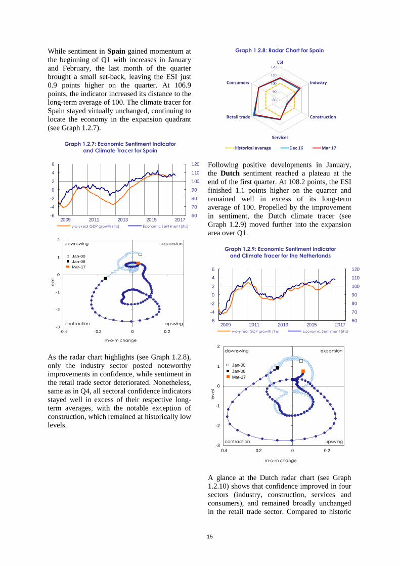

ISBN 978-92-79-64782-6
KC-BF-17-015-EN-N