Embed Size (px)
Citation preview

February 2, 2011
Euclidean Field TheoryKasper Peeters & Marija Zamaklar
Lecture notes for the M.Sc. in Elementary Particle Theory at Durham University.

Copyright c© 2009-2011 Kasper Peeters & Marija Zamaklar
Department of Mathematical SciencesUniversity of DurhamSouth RoadDurham DH1 3LEUnited Kingdom
http://maths.dur.ac.uk/users/kasper.peeters/eft.html

1 Introducing Euclidean Field Theory 51.1 Executive summary and recommended literature . . . . . . . . . . . . 51.2 Path integrals and partition sums . . . . . . . . . . . . . . . . . . . . . 71.3 Finite temperature quantum field theory . . . . . . . . . . . . . . . . . 81.4 Phase transitions and critical phenomena . . . . . . . . . . . . . . . . 10
2 Discrete models 152.1 Ising models . . . . . . . . . . . . . . . . . . . . . . . . . . . . . . . . . 15
2.1.1 One-dimensional Ising model . . . . . . . . . . . . . . . . . . . 152.1.2 Two-dimensional Ising model . . . . . . . . . . . . . . . . . . . 182.1.3 Kramers-Wannier duality and dual lattices . . . . . . . . . . . 19
2.2 Kosterlitz-Thouless model . . . . . . . . . . . . . . . . . . . . . . . . . 21
3 Effective descriptions 253.1 Characterising phase transitions . . . . . . . . . . . . . . . . . . . . . 253.2 Mean field theory . . . . . . . . . . . . . . . . . . . . . . . . . . . . . . 273.3 Landau-Ginzburg . . . . . . . . . . . . . . . . . . . . . . . . . . . . . . 28
4 Universality and renormalisation 314.1 Kadanoff block scaling . . . . . . . . . . . . . . . . . . . . . . . . . . . 314.2 Renormalisation group flow . . . . . . . . . . . . . . . . . . . . . . . . 33
4.2.1 Scaling near the critical point . . . . . . . . . . . . . . . . . . . 334.2.2 Critical surface and universality . . . . . . . . . . . . . . . . . 34
4.3 Momentum space flow and quantum field theory . . . . . . . . . . . 35
5 Lattice gauge theory 375.1 Lattice action . . . . . . . . . . . . . . . . . . . . . . . . . . . . . . . . . 375.2 Wilson loops . . . . . . . . . . . . . . . . . . . . . . . . . . . . . . . . . 385.3 Strong coupling expansion and confinement . . . . . . . . . . . . . . 395.4 Monopole condensation . . . . . . . . . . . . . . . . . . . . . . . . . . 39
3

4

1Introducing Euclidean Field Theory
1.1. Executive summary and recommended literature
This course is all about the close relation between two subjects which at first sighthave very little to do with each other: quantum field theory and the theory of criti-cal statistical phenomena. On the one hand, the methods and insight from quantumfield theory have helped tremendously to understand the concept of “universality”in statistical mechanics. This is the fact that the effective theory relevant for longdistance behaviour of statistical systems depends only on a small number of param-eters. On the other hand, the theory of critical phenomena has shed new light on therole of “renormalisation” in particle physics. Meant here is the way in which subtletuning of parameters of the model is required to remove, or make sense of, spuriousinfinities in loop computations. It is the goal of these lectures to explain how thesetwo fields are related.
Given that this course is about the common ground of two quite different disci-plines, it is no surprise that there is a vast literature to help you with many technicaland conceptual issues. The list below is highly incomplete, but you are strongly en-couraged to consult some of these books to get a wider view on the topics discussedhere.
• M. Le Bellac, “Quantum and statistical field theory”, Oxford University Press,1991.Good for a number of explicit computations, though not terribly transparentin its connection between the two fields, at least on first reading.
• J. L. Cardy, “Scaling and renormalization in statistical physics”, CambridgeUniversity Press, 1996.Standard book on the topic, gives a good overview, but is somewhat thin onexplicit computations.
• J. M. Yeomans, “Statistical mechanics of phase transitions”, Oxford UniversityPress, 1992.Very good, compact and explicit book on the statistical aspects of phase tran-sitions.
• J. B. Kogut and M. A. Stephanov, “The phases of quantum chromodynamics:From confinement to extreme environments”, 2004.Mainly focussed on applications to QCD, but contains some good introductorychapters as well.
5

1.1 Executive summary and recommended literature
• A. M. Polyakov, “Gauge fields and strings”, Harwood, 1987. Contemporaryconcepts in physics, volume 3.An original take on many of the topics discussed here, though sometimes a bittoo compact for a first introduction.
• M. H. Thoma, “New developments and applications of thermal field theory”,hep-ph/0010164.Very clear text on quantum field theory at finite temperature, in particularthe connection between the imaginary time and real time formalisms. Alsocontains a number of explicit applications to QCD.
• G. P. Lepage, “What is Renormalization?”, hep-ph/0506330.Lectures on the meaning of renormalisation from the point of view of a particlephysics theorist.
• M. Creutz, “Quarks, gluons and lattices”, Cambridge University Press, 1983.Another very accessible intro to lattice field theory.
• I. Montvay and G. Munster, “Quantum fields on a lattice”, Cambridge Uni-versity Press, 1994.More advanced book on lattice field theory. Good examples on the strong-coupling expansion.
• J. Smit, “Introduction to quantum fields on a lattice: A robust mate”, Cam-bridge Lect. Notes Phys., 2002.Nice and compact book about lattice field theory. Used heavily in the prepa-ration of these lectures.
• J. Zinn-Justin, “Quantum field theory and critical phenomena”, Int. Ser. Monogr.Phys. 113 (2002) 1–1054.A thousand page reference book, not for the faint of heart, and not always or-ganised in the most pedagogical way. Nevertheless, a very good source if youwant to look up details.
• J. Zinn-Justin, “Quantum field theory at finite temperature: An introduction”,hep-ph/0005272.A much smaller set of lectures exposing the relation between finite tempera-ture quantum field theory and statistical mechanics. The first few sections areworth reading as an introduction to the topic.
6

1.2 Path integrals and partition sums
1.2. Path integrals and partition sums
The root of the connection between quantum field theory and statistical systems isthe functional integral (or path integral). This functional integral is closely relatedto an object in classical statistical mechanics: the partition sum. In order to illustratethis, let us briefly recall the quantum mechanics of a non-relativistic particle in thepath integral language.
Let us start with the transition amplitude for such a particle to go from q to q′ intime ∆. It is given by
A(q′, ∆; q, 0) =∫ q(t=∆)=q′
q(t=0)=qDq(t) exp
[ ih
∫ ∆
0
(m2
qi(t)qi(t)−V(q(t)))
dt]
. (1.1)
As you have seen in the course on quantum field theory, this path integral expres-sion can be related to the usual expression for a transition amplitude in the operatorformalism. For a suitable normalisation of the path integral measure, we have
A(q′, ∆; q, 0) = 〈q′| exp[− i
hH∆]|q〉 , with H =
p2
2m+ V(q) . (1.2)
Here |q〉 is a time-independent state in the Heisenberg picture, and H the Hamilto-nian corresponding to the particle action used in (1.1). For the details of this relation,see your favourite quantum mechanics book.
Consider now what happens to the path integral expression if we make a substi-tution t→ −iτ. This is called a Wick rotation (it rotates the integration in the complextime plane by 90, as in the figure). Provided the Lagrangian does not depend ex-plicitly on t (which, in our case, it does not), this changes the path integral weightinto a nice real expression,
A(q′, ∆; q, 0) =∫ q(τ=∆)=q′
q(t=0)=qDq(τ) exp
[− 1
h
∫ ∆
0
(m2
qi(τ)qi(τ) + V(q(τ)))
dτ]
,
(1.3)where the dot now indicates a derivative with respect to τ. Similarly, if we substitute
The Wick rotation in the complex timeplane.
∆→ −i∆ in the operator expression, we get
A(q′, ∆; q, 0) = 〈q′| exp[− 1
hH∆]|q〉 . (1.4)
This expression should make some bells ring. If we would set |q〉 = |q′〉, and sumover all position eigenstates, then (1.4) looks exactly like the expression for the par-tition function Z[β] of a statistical system at inverse temperature β := 1/(kT) givenby β = ∆/h, The quantum mechanical
transition amplitude for a systemwith periodic boundary conditionsis, after summing over allboundary conditions, equal to aquantum statistical partitionfunction, with β↔ ∆/h.
Z[β] = ∑n〈n| exp
[− βH
]|n〉 , (1.5)
where we sum over a complete basis of states. This gives us our first relation be-tween a quantum mechanical transition amplitude with periodic boundary condi-tions and a quantum statistical system at non-zero temperature.
Let us now take a somewhat different look at the exponent in (1.3). We can writeit as
Vstring = −1h
∫ ∆
0
(m2
qi(τ, τ)qi(τ, τ) + V(q(τ)))
dτ , (1.6)
i.e. as the potential energy of a field qi(τ, τ) in two dimensions, where we now viewτ as the time (the total energy would have an additional kinetic term involving τderivatives). The path integral then simply sums over time-independent configu-rations of this field. We thus see that we can also interpret (1.3) as computing the
7

1.3 Finite temperature quantum field theory
partition function of a classical string of length ∆, at an inverse temperature β = 1/h.This gives us our second relation, between a quantum mechanical transition functionfor a particle and a classical statistical system for a string.The transition amplitude for a
quantum particle for a time −i∆ isequal to the classical partitionfunction of a string of length ∆,with β↔ 1/h.
The second of these relations is easily generalised to quantum field theory. In aLorentzian field theory, the “generating functional in the presence of a source” takesthe form
Z[J] =∫Dφ exp
[ih
S[φ] +∫
dd+1x J(x)φ(x)− ε
h
∫dd+1x φ(x)2
]. (1.7)
where S[φ] is the action corresponding to the field φ. We have included a damping(end of lecture 1)factor dependent on ε, which ensures that field configurations which do not fall offat space-like and time-like infinity are suppressed in the path integral. This ensuresthat all correlation functions which we compute from Z[J] are correlation functionsin the vacuum state, e.g.
〈0| T(
φ(x)φ(y))|0〉 = 1
Z[J]δ
δJ(x)δ
δJ(y)Z[J]
∣∣∣J=0
. (1.8)
We can now do a Wick rotation, and then interpret the exponent in (1.7) as the po-tential of a field φ in one extra dimension. The path integral then computes for usthe classical partition sum of a model at inverse temperature β = 1/h.
The first relation is a bit more tricky to generalise to field theory, because of theexplicit dependence of the statistical model on the time interval. In field theory weusually take the time interval to ±∞. Moreover, we never consider arbitrary fieldconfigurations at the endpoint of this time interval, but rather force the field to sitin the vacuum state. So summing over boundary conditions does not produce ansensible object in quantum field theory. However, what we can do is turn the firstrelation around, and use it to describe a quantum field theory at finite temperaturein terms of a Euclidean path integral. This is the topic of the next section.
I Summary: The generating functional of a Euclidean quantum field theory in dspace dimensions can alternatively be interpreted as a partition sum in a classicalstatistical model in d dimensions. The corresponding inverse temperature is thenrelated to Planck’s constant by β ∼ 1/h.
I See also: Discussions like these can be found in many places, e.g. chapter 2 of thebook by Smit [10] or chapter V.2 of the book by Zee [13].
1.3. Finite temperature quantum field theory
In standard quantum field theory courses one almost always works with systems atvanishing temperature. That is to say, the state which is used to define all correlationfunctions is taken to be the vacuum state |0〉 of the free theory, with no particles. Thepropagator, for instance, is defined as
GF(x− y) = 〈0| T(
φ(x)φ(y))|0〉 . (1.9)
However, we can certainly also construct a quantum theory of fields in which we usea thermal state instead of the no-particle vacuum. Instead of computing a vacuumexpectation value, we then have to compute
GT>0F (x− y) =
∑n〈n| T
(φ(x)φ(y)
)|n〉 e−βEn
∑n
e−βEn. (1.10)
8

1.3 Finite temperature quantum field theory
Here |n〉 is an eigenstate of the Hamiltonian with eigenvalue En. Such states aregenerically complicated multi-particle states. As particles can be created with anythree-momentum, and in any number, they take the form
∣∣n1, . . . , nM;~k1, . . . ,~kM⟩=
M
∏i=1
(a†(~ki)
)ni√ni!
|0〉 . (1.11)
This state has ∑i ni particles, and the generic label n that appears in (1.10) is seen todescribe both the set of momenta that appear, as well as the number of particles ofeach momentum.
We will leave this expression for the time being, and instead ask the questionwhether we can write (1.10) back in a path integral language. It is not immediatelyclear how to do this, because the Gaussian factor in the path integral (1.7) enforcesthe appearances of the |0〉 state in the correlator. The way to continue is to observethat (1.10) is an expression similar to (1.4). We can thus take it from there, andgo backwards, i.e. rewrite the thermal sum over energy eigenstates in terms of apath integral, as we did for the non-relativistic particle. We view the right-handside of (1.10) as a propagator for a field theory over a compact Euclidean time withperiod β, with periodic boundary conditions in this direction.
In fact, this additional Euclidean direction is simply the imaginary part of thetime coordinate which is already present in xµ and yµ. That is to say, the Greenfunction (1.10) is periodic under a shift of the time difference by −ihβ:
GT>0F (x0,~x; 0,~y) =
1Z
Tr[e−βHT
(φ(x0,~x)φ(0,~y)
)]=
1Z
Tr[e−βH φ(x0,~x)φ(0,~y)
](assuming x0 > 0)
=1Z
Tr[φ(0,~y)e−βH φ(x0,~x)
]=
1Z
Tr[e−βHeβH φ(0,~y)e−βH φ(x0,~x)
]=
1Z
Tr[e−βHT
(φ(x0,~x)φ(−ihβ,~y)
)]= GT>0
F (x0,~x;−ihβ,~y) .
(1.12)
The last step, in which we re-introduce time-ordering, requires that we can comparex0 with −ihβ. That is possible if x0 = −iτ, i.e. if the time coordinate was imaginaryto start with. The derivation thus goes through only for correlation functions whichare independent of the real time. For time-dependent situations, we need what iscalled the real-time formalism for thermal quantum field theory, which goes beyondthe Euclidean Field Theory concepts which we focus on in these lectures.
I Summary: The static properties of a quantum field theory at finite temperature canbe obtained by doing a Wick rotation and imposing periodic boundary conditionsin imaginary time.1 The periodic boundary conditions of the path integral corre-spond to the trace of the thermal sum, and the period corresponds to the inversetemperature ∆τ ↔ β.
I See also: The lectures by Thoma [6].
1You may have heard about Hawking radiation of black holes, and the fact that it has a certaintemperature. The simplest way to see that black holes have a temperature is by looking at the analyticcontinuation of a black hole metric in the complex plane. It turns out that the imaginary part of timeneeds to be compact, and hence that any field theory on top of the black hole background is in a thermalstate.
9

1.4 Phase transitions and critical phenomena
1.4. Phase transitions and critical phenomena
Although we have quickly stepped over the relation between the path integral andthe quantum mechanical transition amplitude, a crucial ingredient in the derivationof that relation is a proper definition of the path integral measure. The infinite-dimensional integral is only well-defined if we regularise the model somehow, forinstance by putting it on a lattice (which, in the quantum-mechanical model, meansdiscretising time). As a result, all the systems that we are dealing with in theselectures are in a sense discrete systems, with a countable number N of degrees offreedom. The main question we are then interested in is how such systems behavewhen we change their parameters, when we change the lattice spacing, and whenwe take the thermodynamic limit N → ∞.
From statistical systems, we know that many interesting things can happen. Toillustrate some of these, let us focus on an example which will return several moretimes during these lectures: the Ising model. This model has its roots in the searchfor a simple model which describes a ferromagnet. The main property of a ferro-magnet is that it retains its magnetisation in the absence of an external magneticfield. However, for sufficiently large temperature, this magnetisation disappears.(end of lecture 2)
The key ingredient is the interaction between the electron spins at different sitesof the atomic lattice. A simple model of this type is the Heisenberg model, with Hamil-tonian operator
HHeisenberg = −J ∑〈i,j〉
~σi ·~σj , J > 0 . (1.13)
Here the~σi are the Pauli matrices acting on the spin degrees of freedom at site i. Thenotation 〈i, j〉 indicates a pair of spins at site i and j. Unfortunately, this model canonly be solved on a one-dimensional lattice (Bethe 1931). In that case, for J > 0 theground state is one in which all spins are aligned (while for J < 0 the ground state isthe so-called Neel state, with alternating spins). Even in the classical limit, in whichwe replace the spin operator~σi at each site by a classical three-vector ~Si, the modelis not solvable except in one dimension.
The Ising model incorporates one last simplification, namely the reduction ofthe three-vector at each site to a simple scalar Si, which can take the values ±1. Itsclassical Hamiltonian, in the presence of an external magnetic field, reads
HIsing = −J ∑〈i,j〉
SiSj − h ∑i
Si . (1.14)
This model was introduced by Lenz in the 1920’s, and solved by Ising in the one-dimensional case. In the absence of a magnetic field h, the model was solved byOnsager in two dimensions. No other exact solutions are known.
The parameters of this model are thus the coupling J, the external field h andthe number of sites N. All distances between spins are determined by the latticespacing a (which in this simple model does not actually appear in the Hamiltonian).The partition sum, finally, adds the temperature T to the set of parameters. What wewant to learn is how we can do measurements on this system, how we can expressthose measurements in terms of J, h, N, a and T, and how these behave when wevary the parameters and take the N → ∞ limit. This same story holds for all theother discrete models that appear in these lectures.
What are the observables which we can measure in a statistical model of thetype (1.14)? In general, these are correlation functions, just like in a quantum fieldtheory. The simplest correlation function is the expectation value of a single spin,which is called the local magnetisation. The expectation value of the sum of all spins
10
1.4 Phase transitions and critical phenomena
is the total magnetisation,2
M :=
∑Si
[(∑
iSi)e−βHIsing[Si]
]∑Si
e−βHIsing[Si]. (1.16)
Naively, one would perhaps be tempted to say that M = 0 when the backgroundmagnetic field h vanishes: for every configuration Si there exists another config-uration in which all the spins are flipped, and these two configurations contributewith opposite sign to the partition sum.
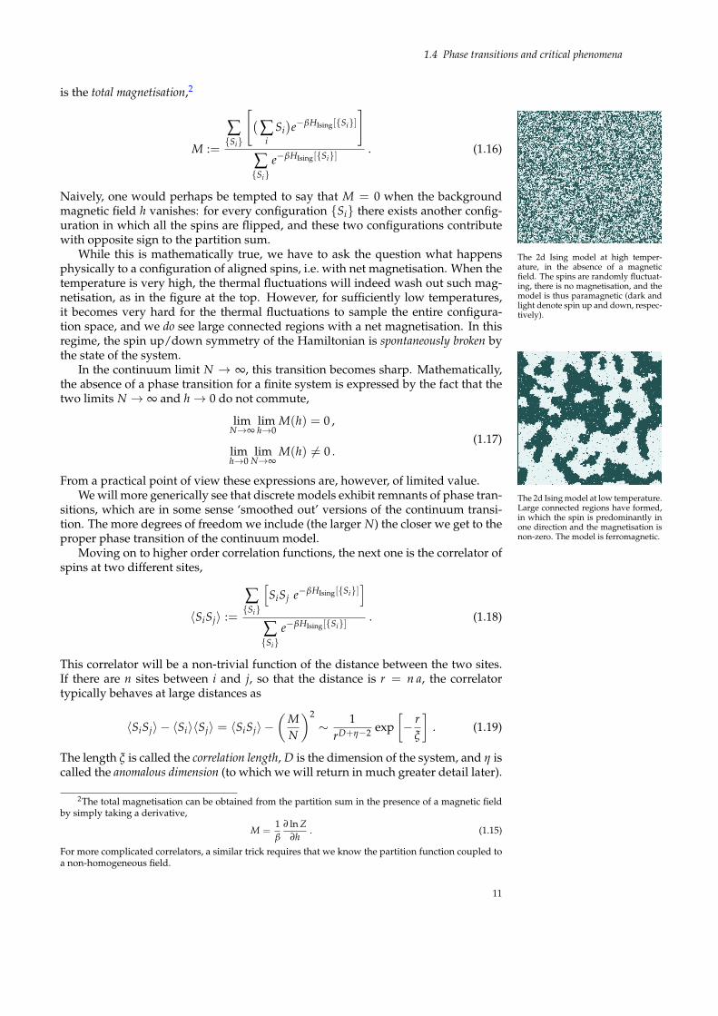
The 2d Ising model at high temper-ature, in the absence of a magneticfield. The spins are randomly fluctuat-ing, there is no magnetisation, and themodel is thus paramagnetic (dark andlight denote spin up and down, respec-tively).
While this is mathematically true, we have to ask the question what happensphysically to a configuration of aligned spins, i.e. with net magnetisation. When thetemperature is very high, the thermal fluctuations will indeed wash out such mag-netisation, as in the figure at the top. However, for sufficiently low temperatures,it becomes very hard for the thermal fluctuations to sample the entire configura-tion space, and we do see large connected regions with a net magnetisation. In thisregime, the spin up/down symmetry of the Hamiltonian is spontaneously broken bythe state of the system.
In the continuum limit N → ∞, this transition becomes sharp. Mathematically,the absence of a phase transition for a finite system is expressed by the fact that thetwo limits N → ∞ and h→ 0 do not commute,
limN→∞
limh→0
M(h) = 0 ,
limh→0
limN→∞
M(h) 6= 0 .(1.17)
From a practical point of view these expressions are, however, of limited value.The 2d Ising model at low temperature.Large connected regions have formed,in which the spin is predominantly inone direction and the magnetisation isnon-zero. The model is ferromagnetic.
We will more generically see that discrete models exhibit remnants of phase tran-sitions, which are in some sense ‘smoothed out’ versions of the continuum transi-tion. The more degrees of freedom we include (the larger N) the closer we get to theproper phase transition of the continuum model.
Moving on to higher order correlation functions, the next one is the correlator ofspins at two different sites,
〈SiSj〉 :=
∑Si
[SiSj e−βHIsing[Si]
]∑Si
e−βHIsing[Si]. (1.18)
This correlator will be a non-trivial function of the distance between the two sites.If there are n sites between i and j, so that the distance is r = n a, the correlatortypically behaves at large distances as
〈SiSj〉 − 〈Si〉〈Sj〉 = 〈SiSj〉 −(
MN
)2∼ 1
rD+η−2 exp[− r
ξ
]. (1.19)
The length ξ is called the correlation length, D is the dimension of the system, and η iscalled the anomalous dimension (to which we will return in much greater detail later).
2The total magnetisation can be obtained from the partition sum in the presence of a magnetic fieldby simply taking a derivative,
M =1β
∂ ln Z∂h
. (1.15)
For more complicated correlators, a similar trick requires that we know the partition function coupled toa non-homogeneous field.
11

1.4 Phase transitions and critical phenomena
As is clear from the figures, the correlation length becomes large when we approachthe phase transition, and we will see that it in fact diverges in a very particular wayas we approach the critical temperature.
We will often use a thermodynamical language to describe the large-distancebehaviour of statistical systems. Without trying to include a full course on ther-modynamics, let us briefly recall some essential concepts. The basic quantity weneed is the entropy. At the microscopic level, it is defined in terms of the number ofmicrostates Ω given the macroscopic parameters (like magnetisation),
S := kB ln Ω . (1.20)
It can also be expressed in terms of the probability of a single state p(Si) to occur,using Shannon’s formula,
S = −kB ∑Si
p(Si) ln[
p(Si)]
. (1.21)
This allows us to relate the entropy to the energy and eventually to the partitionfunction, as we have
p(Si) =1Z
exp[− βH(Si)
], Z = ∑
Siexp
[− βH(Si)
]. (1.22)
All of thermodynamics follows from this microscopic starting point, together withthe laws of thermodynamics.
The second law of thermodynamics states that a system out of equilibrium willeventually evolve to an equilibrium in which the entropy is at least as large as before.If we have two connected systems at energy EA and EB respectively, equilibrium willbe reached when the total entropy reaches an extremum, i.e. when
dStot
dEA
∣∣∣∣eq.
= 0 . (1.23)
This leads to the fundamental definition of temperature in terms of entropy,
T :=(
dSdE
)−1. (1.24)
From here, all the other usual thermodynamical potentials follow by making useof the first law of thermodynamics, which essentially expresses that energy is con-served. The change in internal energy of a system is related to the heat absorbtionand the performed work as
dU = δQ− δW . (1.25)
In terms of state functions, this gives
dU = TdS− PdV + hdM . (1.26)
This expression holds true for a closed system. If the external parameters S andV are fixed, the system in thermodynamical equilibrium will be determined by aminimum of the internal energy U.
However, we often deal with open systems, which are coupled to a heat bathwhich can provide an arbitrary amount of energy to keep the temperature T con-stant. In this case, the energy flow means that S is no longer constant. The secondlaw now imposes that a minimum is found for
F = U − TS− hM . (1.27)
12

1.4 Phase transitions and critical phenomena
This quantity F is the Helmholtz free energy, and we can relate it to the partitionfunction by making use of (1.21),
S = −kB ∑Si
1Z
exp[− βH
](− βH − ln Z) = kB
[β(U − hM) + ln Z
], (1.28)
so that we find (end of lecture 3)F = −kBT ln Z . (1.29)
There are also thermodynamic potentials which are relevant when the pressure iskept fixed (and thus the volume is allowed to change), but these are not very rel-evant for systems like the Ising model. For completeness, they are all listed in thetable below.
Internal energy U(S, V, M) dU = TdS− PdV + hdM
Helmholtz free energy F(T, V, h) = U − TS− hM dF = −SdT − PdV −Mdh
Gibbs free energy G(T, P) = F + PV
Enthalpy H(S, P) = U + PV
In the last column of this table, you can see how the potentials change when theparameters are modified.
I See also: A more extensive explanation of entropy and free energy can be foundin [14].
13

1.4 Phase transitions and critical phenomena
14

2Discrete models
As announced, our main interest will be in systems which have a finite number ofdegrees of freedom, either because they are defined on a lattice or because they areobtained by cutting off high-momentum modes of a continuum theory. In chap-ter 4 we will be interested in analysing how such systems behave when we send thelattice spacing to zero, or remove the cutoff. For the time being, however, we areinterested in analysing the discrete models by themselves.
2.1. Ising models
2.1.1 One-dimensional Ising modelWe have already seen the Ising model Hamiltonian,
HIsing = −J ∑〈i,j〉
SiSj − h ∑i
Si . (2.1)
The partition function Z[β, J, h] for the one-dimensional model is then given by
Z = ∑Si=±1
N−1
∏i=0
exp[
β(
JSiSi+1 +12
h(Si + Si+1))]
. (2.2)
It can be computed by a method known as the transfer matrix method. For thispurpose, we make the spin chain periodic, i.e. the spin to the right of SN−1 is S0again. The partition can then be expressed as the trace of a product of 2× 2 matrices,
Z = ∑Si=±1
TS0S1 TS1S2 · · · TSN−1S0 ,
where TSiSj = exp[
β(
JSiSj +12
h(Si + Sj))]
. (2.3)
The matrix T is the transfer matrix. This procedure is in spirit very similar to theway in which we derive the path integral from the quantum mechanical transitionamplitude: we cut up the amplitude in a number of steps, glue those steps together,and sum over the states at the intermediate points. Here that sum over ‘intermediatestates’ is given by the sum over spins.
In more explicit form, we can write the matrix elements of T as
T =
(eβ(J−h) e−βJ
e−βJ eβ(J+h)
). (2.4)
15

2.1 Ising models
Since the trace of a matrix is equal to the sum of its eigenvalues, we can express thepartition sum as
Z = Tr[
TN]= λN
+ + λN− , (2.5)
where λ± are the eigenvalues of T, with λ+ > λ−. It is not hard to compute theseeigenvalues explicitly; from (2.4) we get
λ± = eβJ(
cosh(βh)±√
sinh2(βh) + e−4βJ)
. (2.6)
When we take the continuum limit N → ∞, the largest of these two eigenvalues willtend to dominate the physics.
We can immediately compute a number of observables, following the generallogic outlined in section 1.4. The simplest is the free energy F. In the N → ∞ limit,this one becomes
F = −kBTN ln λ+ = −JN − kBTN ln(
cosh(βh) +√
sinh2(βh) + e−4βJ)
. (2.7)
It is an extensive quantity (scaling with the size of the system), but the strict linearThe free energy in the continuumlimit is determined by the largesteigenvalue of the transfer matrix.
scaling with N holds true only in the large-N limit. When h = 0 this reduces to
F = −kBTN ln [2 cosh(βJ)] . (2.8)
This is an analytic function in T except at T = 0. Hence there is no phase transitionin the one-dimensional Ising model.
The next quantity is the magnetisation. We can compute this in two differentways. Given that we already have the free energy, we can compute it simply byusing
M = −(
∂F∂h
)T= N
sinh(βh)√sinh2(βh) + e−4βJ
. (2.9)
We can alternatively compute it by doing a direct computation of the expectationvalue of the sum of spins (this method will prove useful later when we computethe correlation length). Since the system is translationally invariant, we can simplycompute the expectation value of a single spin and multiply that with N, to get
M = N〈Sk〉 =NZ ∑Si
TS0S1 TS1S2 · · · TSk−1Sk × Sk × TSkSk+1 · · · TSN−1S0
= NTr[
TkSTN−k]
Tr[
TN] = N
Tr[S TN
]Tr[
TN] , where S :=
(−1 00 1
). (2.10)
Translation invariance is reflected in the fact that this result is independent of k, andrelated to the cyclic invariance of the trace. In order to compute the trace on theright-hand side of (2.10), we note that T is a symmetric matrix and hence can bediagonalised with an orthogonal matrix P,
T = PΛP−1 , where Λ =
(λ− 00 λ+
). (2.11)
If we find P, we can then compute the magnetisation using
M = NTr[
P−1SP ΛN]
Tr[ΛN] . (2.12)
16

2.1 Ising models
By writing out the right-hand side of (2.11) explicitly and comparing with the com-ponents of T on the left-hand side, one finds that
P =
(cos φ − sin φsin φ cos φ
), with cos(2φ) =
sinh(βh)√sinh2(βh) + e−4βJ
. (2.13)
We then get
-3 -2 -1 1 2 3h
-1.0
-0.5
0.5
1.0
M
The magnetisation of the one-dimensional Ising model as a functionof the external magnetic field. Theflatter curves correspond to highertemperatures.
P−1SP =
(− cos(2φ) sin(2φ)
sin(2φ) cos(2φ)
),
M = N(λN
+ − λN−) cos(2φ)
λN+ + λN
−
N→∞−→ N cos(2φ) , (2.14)
which together with (2.13) reproduces the result obtained in (2.9). Note that forh = 0 the magnetisation is always zero, indicating that there is indeed no phasetransition in the one-dimensional Ising model. A plot of the magnetisation as afunction of the external field, for various values of the temperature, is given in thefigure. (end of lecture 4)
The correlation length can now be computed using a very similar technique.
〈S0Sr〉 =1Z ∑Si
S0 × TS0S1 TS1S2 · · · TSr−1Sr × Sr × TSrSr+1 · · · TSN−1S0
=Tr[STrSTN−r
]Tr[
TN] =
Tr[S (PΛrP−1)S(PΛN−rP−1)
]Tr[
TN] , (2.15)
Here Λ is again the matrix of eigenvalues as given in (2.11). In the large-N limitthe ΛN matrix can be approximated by keeping only the largest eigenvalue λ+, butbecause r is finite, the Λr matrix depends on both eigenvalues. A bit of matrixmultiplication yields
〈S0Sr〉 = cos2(2φ) +
(λ−λ+
)rsin2(2φ) . (2.16)
Using our previous result for the magnetisation, the variance becomes
〈S0Sr〉 − 〈S0〉〈Sr〉 =(
λ−λ+
)rsin2(2φ) . (2.17)
The only r-dependence sits in the ratio of eigenvalues. From the definition of the 0.0 0.2 0.4 0.6 0.8 1.0 1.2 1.4h
0.5
1.0
1.5
2.0
2.5
3.0
3.5
Ξ
The correlation length of the one-dimensional Ising model as a functionof the external magnetic field. Again,the flatter curves correspond to highertemperatures.
correlation length (1.19) we then find
ξ ∝1∣∣ln (λ−/λ+
)∣∣ , η = 1 . (2.18)
At zero external magnetic field the correlation length reduces to ξ = 1/ ln tanh(βJ).The behaviour as a function of the magnetic field is plotted for various temperaturesin the figure.
We state here without proof that for many other models, the correlation lengthis determined by the same type of expression (2.18), with λ+ and λ− the two largest The correlation length is
determined in terms of the twolargest eigenvalues of the transfermatrix.
eigenvalues of the transfer matrix. Note that if λ− = 0 the correlation length van-ishes. This happens when J = 0, i.e. when there is no interaction between the spins.
17

2.1 Ising models
A phase transition happens when ξ → ∞, which requires that the two largesteigenvalues become degenerate. For the one-dimensional Ising model this only hap-pens when h = 0 and β→ ∞ (T → 0), but this does not connect two phases.
I See also: The one-dimensional Ising model is discussed in many places, seee.g. [15].
2.1.2 Two-dimensional Ising modelThe two-dimensional Ising model can also be solved by the transfer matrix tech-nique, as was shown by Onsager in 1944. However, this requires a much more sub-
The unique configuration whichchanges 4 bounds (multiplicity N).
stantial analysis. Instead, we will in these lectures use a different method to extractproperties of the two-dimensional model. This goes under the name of Kramers-Wannier duality, and is a relation between the low-temperature perturbative expan-sion and the high-temperature perturbative expansion. The advantage of doing thisis that such expansions and duality relations have analogues in all of the other sys-tems which we will discuss, and hence these techniques are of more general use (incontrast to the transfer matrix method which, although it can sometimes give exactresults, is in general too complicated to be of any use). We will in this section onlyconsider the case of a vanishing external magnetic field, i.e. h = 0, and for the timebeing just look at the low- and high-temperature expansions in isolation.
For the low-temperature expansion, we start with the ground state at T = 0, whichhas all spins in one direction (here taken to be ‘up’). We have to sum over all config-urations in the partition sum. For low temperature, the more spins we flip the morebonds will change their energy, and hence we can look at things order by order in thenumber of flipped spins. If we flip one spin, 4 bonds are changed. Each such bondyields an energy increase of 2βJ. If we flip two spins, we can do it in two differentways, depending on how close the spins are. For the first possibility (top figure) wecan place this at any of the N lattice sites, but there are two orientations, so there are2N possibilities, each changing 6 bonds. For the second possibility (bottom figure)we have N(N− 5)/2 possible ways of placing it, and we change 8 bonds. There arethree other configurations which change 8 bonds, obtained by flipping more spins.For the partition sum, we obtain the low-temperature expansion,
Z = e2NβJ(
1 + Ne−8βJ + 2Ne−12βJ +12
N(N + 9)e−16βJ + · · ·)
. (2.19)
Here e2NβJ is energy of the all-up state (explained by the fact that there are 2 linksfor every site, e.g. the one pointing up and to the right). Since T is small, βJ is largeand hence e−βJ is a small number.
Let us now turn to the high-temperature expansion. When T is large, βJ is small.A crucial role in finding an expansion in small βJ is played by the following sim-ple identities, valid for a variable S which takes values ±1 (and easily verified byinserting S = ±1 explicitly),
eβJS = cosh(βJ) + S sinh(βJ) , ∑S=±1
Sn =
0 if n odd
2 if n even .(2.20)
Using these identities we can rewrite the partition sum in the following form,
Configurations which change 6 bonds(top figure, multiplicity 2N) or 8 bonds(other figures, multiplicity 1
2 N(N − 5),2N, 4N and N respectively).
Z = ∑Si=±1
∏〈i,j〉
(cosh(βJ) + SiSj sinh(βJ)
)
=[
cosh(βJ)]2N
∑Si=±1
∏〈i,j〉
(1 + SiSj tanh(βJ)
). (2.21)
18

2.1 Ising models
At this stage we have not done any approximation yet, we have just rewritten thepartition sum in a somewhat different form. However, note that tanh(βJ) is smallat high temperature. We can thus use (2.21) to attempt an expansion in powers oftanh(βJ). (end of lecture 5)
If we expand (2.21) in powers of tanh(βJ), the only terms which contribute arethose in which all spins which occur do so in even powers (by virtue of the identitiesin (2.20)). It is convenient to think about such terms in a graphical way, since thatwill help us to count the number of terms at each order. To do this, first observe thatin the expression (2.21), a given product of two spins SnSm appears only once. If wedenote this product by a line from site n to site m, we need to look for those graphs inwhich the contours are closed, i.e. do not end in a single spin factor. Multiple closedcontours are allowed though. Every line segment contributes a power of tanh(βJ),and the total contour length thus sets the order in the perturbative expansion. Forthe partition sum we find
Z =(
cosh βJ)2N
2N(
1 + N(tanh βJ)4 + 2N(tanh βJ)6
+12
N(N + 9)(tanh βJ)8 + · · ·)
. (2.22)
The main idea behind the high-temperature expansion we have just seen is thattheir are only nearest-neighbour couplings in the Hamiltonian. These couplings arethe lines in our graphs, and what the high-temperature expansion does is to grouplattice variables into linked clusters. For this reason, it is also known as the clusterexpansion or hopping expansion. We will see that it has its use also in much morecomplicated discrete models, like lattice gauge theory.
2.1.3 Kramers-Wannier duality and dual latticesBoth the low-temperature and high-temperature expansions of the two-dimensionalIsing model partition sum are untransparent and complicated. However, we see thatthese two perturbative series get transformed into each other if we simultaneouslyreplace
e−2βJ ↔ tanh(βJ) ,
Zlow
e2NβJ ↔Zhigh
2N(cosh βJ)2N .(2.23)
This is a remarkable property. It says that if we understand the low-temperature,magnetised phase of the model, we will also understand the high-temperature, dis-ordered phase. As we will see shortly, this symmetry is not just a property of the
Various closed contours with non-overlapping edge segments. In thethird figure, there are N ways to putthe first square and N − 5 to put thesecond (since the 5 squares denoted byred dotted lines are disallowed). Themultiplicities are N, 2N, 1
2 N(N − 5),2N, 4N and N respectively.
first few terms in the perturbative expansions. In fact, it is possible to start witha partition sum Z[β], and rewrite it such that it looks like the partition sum of theIsing model at a different temperature, Z[−(1/2) ln tanh(βJ)]. More precisely,
Z[β] =[
sinh(2βJ)]−N× Z[β] , (2.24)
where β and β are related by the relation we found from the perturbative analysis,
βJ = −12
ln tanh(βJ) . (2.25)
The two-dimensional Ising model is called self-dual, in the sense that we can rewrite The two-dimensional Ising modelis self-dual.its partition function as that of another two-dimensional Ising model, but at a dif-
ferent temperature.
19

2.1 Ising models
If we assume that the system has only one phase transition, then this had betterhappen when the inverse temperatures β and β are the same. This requires(end of lecture 6)
sinh(2βc J) = 1 ⇒ Tc =2J
kB ln(1 +√
2). (2.26)
Even though we have not yet shown that there is in fact a phase transition, wealready know that it has to happen at this particular critical temperature. No exactsolution of the model was required.
In this particular case, the result (2.26) for the critical temperature can be veri-fied by making use of Onsager’s solution of the two-dimensional Ising model usingtransfer matrix techniques. Needless to say, it agrees with the explicit computation.
Let us now look closer at how the exact duality (2.24) can be proven. What wewant to show is how the Ising model partition sum can be rewritten in terms ofanother partition sum, but at a different temperature. The starting point is the fullexpression for the partition sum at vanishing magnetic field. Setting J = 1 (as onlythe combination βJ appears), this is
Z = ∑Si
exp[
β ∑〈i,j〉
SiSj
]. (2.27)
The first step is to rewrite this expression in a way similar to what we did in the firststep of the high-temperature treatment, now written in a somewhat more compactform,
Z = ∑Si
∏〈i,j〉
∑kij=0,1
Ckij(β)(SiSj)
kij ,
where C0(β) = cosh β , C1(β) = sinh β . (2.28)
The new variables kij are associated to every nearest-neighbour pair, i.e. to everylink on the lattice (they are link variables). As we already noted earlier, the only con-tributions to this sum are those which have an even power of each spin variable Si.This means that the only non-zero contributions are those in which the distributionof values of the link variables is such that the sum of all links connected to each andevery spin Si is an even number. If it is, the sum over Si will yield twice the samecontribution ‘one’, so that we can simplify Z as
Z = ∑kl
∏l
Ckl(β)∏
i2 δ(sum of values of links incident at i modulo 2) . (2.29)
In other words, we have rewritten the partition sum as a sum over the link variables,but these link variables have to satisfy a particular constraint.
The trick to solve this constraint is to realise that there is yet another set of vari-ables which we can introduce, such that the link constraint is always satisfied. These
The original Ising lattice (open dots) to-gether with the dual lattice (filled dots).Also indicated are the four links inci-dent on S1, one of which is k12. Thedual variables S1 and S2 are used to de-fine k12.
are the dual variables Si, which sit on the nodes of the dual lattice, as indicated in thefigure. The link variables are related according to
k12 =12(1− S1S2) , (2.30)
and so on. For the sum of the four link variables incident at S1, this gives
2− 12(S1S2 + S2S3 + S3S4 + S4S1) = 2− 1
2(S1 + S3)(S2 + S4) . (2.31)
This expression is manifestly even for any choice of dual variables.
20

2.2 Kosterlitz-Thouless model
So we can now write the partition function as
Z =12
2N ∑Si
∏〈i,j〉
C(1−Si Sj)/2(β) . (2.32)
The extra factor of 1/2 arises because there are two configurations of dual variableswhich give rise to the same value of the link variable, and thus all configurations oflink variables are counted twice. The only thing that is left is to express the Ck(β) interms of the dual variables. This gives
Ck(β) = cosh β(1 + k(tanh β− 1)
)= cosh β exp
[k ln tanh β
]= (cosh β sinh β)1/2 exp
[− 1
2 SiSj ln tanh β]
.
(2.33)
If we insert this into the partition sum we arrive at
Z =12(2 cosh β sinh β)N ∑
Siexp
[− 1
2 ln tanh β ∑〈i,j〉
SiSj]
=12(sinh 2β)−N ∑
Siexp
[β ∑〈i,j〉
SiSj]
. (2.34)
This is again an Ising model, now in terms of the dual variables, and with a cou-pling β which is related to the original one by the relation we found earlier in theperturbative analysis, namely β = −(1/2) ln tanh β.
I See also: A good text on duality in statistical systems and field theory is Savit’sreport [16]. The Ising model is discussed in e.g. [3].
2.2. Kosterlitz-Thouless model
The next model we will discuss is the Kosterlitz-Thouless model. It is again a latticemodel, but instead of the spin variables Si of the Ising model, which can only takeon the values ±1, it has a two-dimensional unit-vector ~S at each site. That is to say,there is one continuous angle variable at each site, with
~Si =(
cos θi, sin θi)
. (2.35)
It is thus the same as the classical Heisenberg model in two dimensions. The Hamil-tonian is again given by a nearest-neighbour one,
HKT = −J ∑〈i,j〉
~Si · ~Sj = −J ∑〈i,j〉
cos(θi − θj
)(2.36)
The crucial ingredients which set this model apart from the Ising model is that weare dealing with a continuous variable, and that this continous variable is periodic,i.e. takes values in a compact space. These properties will come back again whenwe discuss lattice gauge theories for QCD, so the Kosterlitz-Thouless model is a nicewarm-up example.
One might perhaps have expected that, just like for the Ising model, there shouldbe a high-temperature phase in which the spins are disordered and there is no mag-netisation, and a low-temperature phase in which the spins align and there is a net
21

2.2 Kosterlitz-Thouless model
magnetisation (the expectation value of the sum of spins does not vanish). However,that intuition turns out to be wrong. What we will see is that the Kosterlitz-Thoulessmodel never has a net magnetisation, but it does exhibit two different phases, char-acterised by two different behaviours of the correlation function 〈~Si~Sj〉.(end of lecture 7)
At high temperature, we can make an expansion which is very similar to the onein the Ising model. Write the correlation function as
〈eiθ0 e−iθn〉 = 1Z
∫∏m
dθm eiθ0−iθn × exp
12
βJ ∑〈i,j〉
(eiθi−iθj + eiθj−iθi
) . (2.37)
Here we have expanded the cosine in terms of exponentials. For large tempera-tures, we can expand in powers of β and obtain integrals over exponentials. Usingidentities which take the role of those in (2.20),∫ 2π
0dθm = 2π ,
∫ 2π
0dθmeiθm = 0 , (2.38)
we then see (again by similar logic as in the Ising model at high temperature) thatthe only terms which will contribute to the correlator are those in which we haveexponentials corresponding to a contour which starts at site 0 and ends at site n.Any other contour will have a left-over eiθk for some site, and integrate to zero.Assuming that the sites 0 and n are on an axis, the lowest order contribution comesfrom a contour that goes straight between these sites, and is of order (βJ)n. Thecorrelator thus behaves as
〈eiθ0 e−iθn〉 ∼ exp[− |n| ln
(1/(βJ)
)]. (2.39)
The correlation length is thus ξ ∼ 1/ ln(1/(βJ)
)at high temperature.The Kosterlitz-Thouless model at
high temperature has a finitecorrelation length, which goes tozero as T → ∞.
In the low-temperature phase we expect the phases θn to vary slowly as a func-tion of the position on the lattice. We can then expand the cosine in the Hamiltonian,and obtain for the correlator
〈eiθ0 e−iθn〉 = 1Z
∫∏m
dθm eiθ0−iθn exp
βJ − 12
βJ ∑〈i,j〉
(θi − θj)2
. (2.40)
In preparation for the jump to continuum field theories, the argument of the Boltz-mann weight is often interpreted as a discretised derivative, i.e.
12
βJ ∑〈i,j〉
(θi − θj)2 =
12
βJ ∑i,µ(∇µθi)
2 , (2.41)
where µ labels the direction away from site i, and (in a somewhat sloppy notation),
∇µθi := θi+µ − θi . (2.42)
The integral in (2.40) is purely Gaussian, so can be performed exactly. Using thecontinuum language (2.42), we find1
〈eiθ0 e−iθn〉 ∼∣∣∣∣ 1n∣∣∣∣ 1
2πβJ. (2.44)
Since there is no exponential suppression, the correlation length is infinite. How-The Kosterlitz-Thouless model atlow temperature has an infinitecorrelation length, but nospontaneous symmetry breaking.
1This is similar to the manipulation with path integrals, which states that∫Dφ exp
[∫dx( 1
2(∂µφ(x))2 + J(x)φ(x)
)]∝ exp
[12
∫dx∫
dy J(x)∆(x− y)J(y)]
, (2.43)
with ∆(x − y) the inverse of the kinetic operator. In the case here, J(x) = δ(x) − δ(n − x), and thepropagator in two dimensions behaves as ∆(n) ∼ − 1
2π ln |n|.
22

2.2 Kosterlitz-Thouless model
ever, the correlation function does fall off to zero for large distance. Because wehave 〈eiθ0 e−iθn〉 ∼ 〈eiθ0〉〈e−iθn〉 for large distances, this immediately also implies thatthere is no magnetisation, i.e. no spontaneous symmetry breaking. This is in agree-ment with the Coleman-Mermin-Wagner theorem which says that a continuous globalsymmetry in two dimensions cannot be spontaneously broken in a system with localinteractions.
The question now remains: what is the crucial qualitative difference betweenthe low-temperature and the high-temperature regime? The key ingredient is theperiodicity of the θi variables. If we consider the continuum formulation of themodel (using (2.41)), the solutions to the equations of motion are solutions to thetwo-dimensional Laplacian, with an additional periodicity condition,(
∂2x + ∂2
y
)θ = 0 , 0 < θ < 2π . (2.45)
The solutions to this equation can be labelled by the number of times the phase
A vortex of the Kosterlitz-Thoulessmodel, arrows denoting the unit-vectors ~Si .
θ goes around when we circle the origin. These vortices are configurations whichhave a lower free energy for sufficiently high temperatures. They ‘condense’ abovethis Tc, and lead to a finite correlation length.
It is not so easy to show that these vortices indeed dominate the partition sumabove Tc. However, it can be made plausible by estimating the free energy of avortex, and showing that condensation of a vortex lowers the free energy above acertain temperature. The free energy is
F = E− TS , (2.46)
where S is the entropy. The energy can be determined from
E =12
∫d2x (∂µθ)2 =
∫dφdr rgφφ = π J ln(L/a) , (2.47)
where we approximated θ = φ, and have written the answer in terms of the totalsize of the lattice L and the lattice spacing a. Now the entropy is simply given by kBtimes the logarithm of the number of ways in which we can put down the vortex,which is the number of lattice sites (L/a)2. So we find
F =(π J − 2kBT
)ln(L/a) . (2.48)
Above Tc = π J/(2kB) the system prefers to condense a vortex. This is one of theclassic examples of a system in which “entropy wins over energy”. Working outthe precise details of the condensation mechanism goes beyond the scope of theselectures. (end of lecture 8)
I See also: Section 2.5 of [4] for a deeper analysis of vortex condensation in theKosterlitz-Thouless model.
23

2.2 Kosterlitz-Thouless model
24

3Effective descriptions
In the previous chapter we have seen a number of explicit examples of systems witha phase transition. We have, however, not discussed much of the details of phasetransitions themselves, or the techniques to compute properties of these systemsclose to the phase transition. Exact computations are often hard (as witnessed bye.g. the two-dimensional Onsager solution of the Ising model). In the present chap-ter we will introduce two ideas for approximate methods to capture the essentialsof systems with phase transitions. Before we do that, we will however need a littlebit more terminology.
3.1. Characterising phase transitions
A phase transition occurs when the external parameters of a system are such thatone or more obervables are singular (i.e. discontinuous or divergent). These pointsin the phase diagram are called critical points. The critical exponents show how var-ious quantities vanish or diverge near the critical points. An important propertyof phase transitions is that various systems which naively look very different maystill, when they approach the critical point, have identical behavior. More precisely,many different systems turn out to have the same critical exponents. Examples ofsuch systems are the Ising model on a square and triangular lattice. While the valueof the critical temperature depends on the details of the interaction, these two mod-els do turn out to have the same critical exponents.
Phase transitions are commonly classified into roughly three different groups.For first order transitions,
The phase diagram of the two-dimensional Ising model. For T < Tcthe transition between h < 0 andh > 0, along the blue curve, isfirst-order (the magnetisation jumpsdiscontinuously). The line of first-order transitions in the h − T plane(red dashed line) ends in the criticalpoint T = Tc .
1. The singular behaviour is manifest in the form of discontinuities.
2. The correlation length ξ stays finite.
3. The latent heat can be non-zero, i.e. going from one phase to the other canrelease or absorb energy.
4. At the transition two or more phases may coexist in equilibrium (for instance,liquid-ice in water, or domains of magnetisation in ferromagnets).
5. The symmetries of the system in the phases on either side of the transition areoften unrelated.
A first order transition occurs for example in the Ising model below the critical tem-perature (see the figure), when we change the external magnetic field from negativeto positive. Typically, the line of first-order transitions ends in a critical point. If we
25

3.1 Characterising phase transitions
follow a path at zero magnetic field, passing through this point leads to a second-order transition.
Second-order transitions are transitions in which
1. The singular behaviour is visible in the form of divergences.
2. The correlation length ξ diverges.
3. The latent heat is zero.
4. There are no mixed phases at the transition point.
5. The symmetries of the system in the phases on either side of the transitionare related (usually the symmetries for T < Tc form a subgroup of those atT > Tc).
Using again the Ising model as an example, and focussing on h = 0, we see that thespontaneous magnetisation for T < Tc breaks the symmetry of the phase at T > Tc.
Finally, there exist a class of infinite order transitions, in which no symmetries getspontaneously broken. We have actually seen such a transition when we discussedthe Kosterlitz-Thouless model.1
For the purposes of this course, the second-order transitions are most relevant,as the correlation length diverges and the system loses knowledge about the mi-croscopic details. In the language of discretised quantum field theory, adjustingthe parameters such that the correlation length diverges is also known as taking thecontinuum limit. The way in which the correlation length diverges is commonly pa-rameterised by the critical exponent ν, defined asCritical exponents determine the
behaviour of observables near asecond-order phase transition.
ξ ∼∣∣T − Tc
∣∣−ν . (3.1)
In fact, the two-point correlator yields more information than just the correlationlength; recalling the definition (1.19),
〈SiSj〉 − 〈Si〉〈Sj〉 ∼1
rD+η−2 exp[− r
ξ
]. (3.2)
we also have the exponent η, which sets the power-law behaviour of the two-pointcorrelator. The η exponent is called the anomalous dimension. Typically, many othercorrelation functions will diverge too. The first of those is the magnetisation, whichis the order parameter of the phase transition (it can be used to determine whetherwe are in one phase or another). We thus have a number of other standard criticalexponents,Phase transitions are labelled by
the value of one or more orderparameters. specific heat : C ∼
∣∣T − Tc∣∣−α
(at h = 0) ,
order parameter : M ∼∣∣T − Tc
∣∣β (at h = 0) ,
susceptibility : χ ∼∣∣T − Tc
∣∣−γ(at h = 0) ,
equation of state : M ∼ h−1/δ (at T = Tc) .
(3.3)
The specific heat is defined as C = (∂2F/∂T2)V and the susceptibility as χ =(∂M/∂h)T . For systems other than the Ising model, the role of M and h can ofcourse be played by some other parameters. We will see later that not all of thesecritical exponents are independent; they are related by so-called scaling relations.The critical exponents α, β, γ, δ, ν
and the anomalous dimension ηlabel a universality class.
1The naming convention of phase transitions is historical and is vaguely connected to the order inderivatives of the thermodynamic potentials at which a discontinuity is present. This historical detail isbest forgotten.
26

3.2 Mean field theory
Experimentally, it is observed that many quite different systems neverthelesshave the same critical exponents. This goes under the name of universality. Fromthe point of view of the microscopic theory, the existence of such universality classescan be quite suprising. Mean field theory and the Landau-Ginzburg approximationboth explain to some extent why universality exists, and how we can make use of itto compute properties of systems near a phase transition.
3.2. Mean field theory
Mean field theory and Landau-Ginzburg models are phenomenological theorieswhich were developed to describe phase transitions. Both give the same predictionsfor the critical exponents. Both ignore local fluctuations of spins (or other variables)about their mean value. Hence, neither of them give correct critical exponents inlow dimensions, where these fluctuations can be very wild. As the dimension isincreased, the predictions of these theories is improved, and they essentially predictthe correct critical exponents at an ordinary critical point if D > 4. (end of lecture 9)
In the mean-field approach, we are still dealing with the microscopic degreesof freedom, but instead of coupling them to their neighbours, we couple them tothe average ‘field’ produced by all other degrees of freedom. Let us illustrate thisapproach at the level of the Ising model. Recall the Hamiltonian (1.14),
HIsing = −J ∑〈i,j〉
SiSj − h ∑i
Si . (3.4)
The idea is now to write Si = m + δSi, i.e. write the spin as a difference with respectto the average spin. We use this to write
SiSj = −m2 + m(Si + Sj) + δSiδSj . (3.5)
The idea will now be to neglect δSiδSj in all computations (as well as higher orderterms in the variation).2 With this assumption, the Hamiltonian becomes
HMFT = −J ∑〈i,j〉
(−m2 + m(Si + Sj)
)− h ∑
iSi
= JNDm2 − (h + 2JDm)∑i
Si , (3.6)
where we have made use of the fact that in D dimensions, there are D links for eachsite. The partition sum now becomes
ZMFT = exp[−βJNDm2
]∑Si
exp
[β(h + 2JDm)∑
iSi
]
= exp[−βJNDm2
] (2 cosh
(β(h + 2JDm)
))N, (3.7)
where we have used once more the identities (2.20). The free energy becomes
FMFT = N[
JDm2 − kBT ln(
2 cosh(
β(h + 2JDm)))]
. (3.8)
2As the average spin m can be between plus and minus one, the difference δSi can be of order onedepending on the site. However, the idea is that deviations for which this value is large are rare, and formost spins δSi will in fact be small.
27

3.3 Landau-Ginzburg
The magnetisation follows, as in section (2.1.1), either by computing the expec-tation value of the spin directly,
m = 〈Sk〉 =∑Si
Sk exp
[β(h + 2JDm)∑
iSi
]
∑Si
exp
[β(h + 2JDm)∑
iSi
] = tanh(
β(h + 2JDm))
, (3.9)
or by taking the h-derivative of the partition sum. The value for the magnetisationcan be obtained graphically from this equation, see the figure. Plotting the magneti-sation as a function of T then gives us the mean-field approximation to the phasediagram of the Ising model.
-1.5 -1.0 -0.5 0.5 1.0 1.5m
-1.5
-1.0
-0.5
0.5
1.0
1.5
<S>
Solving for the magnetisation of theIsing model in the mean-field approx-imation. At h = 0, there are three solu-tions, m = 0 and m = ±m0.
The critical exponents can be obtained directly. Firstly, the critical point (thattemperature above which (3.9) only has the trivial solution m = 0) is at T = 2DJ/kB.When h = 0 we can expand m near the critical point, to obtain
m ≈ m(1− t)− 13
m3(1− t)3 , (3.10)
where t = (T− Tc)/Tc (so that β ≈ 12DJ (1− t). This leads to m ∼ (−t)1/2 (of course
valid only for t < 0), so that the critical exponent β = 1/2. Similar logic leads to theother critical exponents, γ = 1 and δ = −3.1 2 3 4 5 6 7
T0.0
0.2
0.4
0.6
0.8
1.0
m
Magnetisation of the two-dimensionalIsing model in the mean-field approxi-mation, for h = 0 (positive branch) andh > 0, as a function of temperature.
The mean-field approximation gets several things wrong, in particular the factthat it predicts a second-order phase transition for any dimension (whereas we haveseen that no such transition exists for the one-dimensional Ising model).
3.3. Landau-Ginzburg
The Landau-Ginzburg approximation which assumes that the only relevant degreesof freedom near a phase transition are those which are associated to an order pa-rameter. Concretely, for the Ising model, this means that it attempts to describethe model purely in terms of the average magnetisation m(x) of the spins. In itscrudest form, it assumes that the average magnetisation is the same for all spins, inwhich case it obtains results which are like those of the mean-field approximation.(end of lecture 10)In contrast to that approximation, however, the Landau-Ginzburg approach doesnot explicitly deal with the microscopic degrees of freedom. Rather, the goal is towrite down the most general expression for the free energy as a function of the orderparameter, such that it is compatible with the symmetries of the underlying discretemodel. The idea is that the order parameter is in some sense the ‘slowest’ degree offreedom of the system.
For the Ising model, the underlying system at h = 0 has a symmetry Si ↔ −Si,so the Landau-Ginzburg energy has to be symmetric under a sign flip of m(x). Wewrite
F = F0 + F2m2 + F4m4 + . . . . (3.11)-2 -1 1 2
m
5
10
15
20
25F
Behaviour of the Landau-Ginzburgfree energy for positive, zero and nega-tive value of F2. For negative values,two minima appear, which break thesymmetry.
The value F2 = 0 corresponds to the critical temperature. For F2 > 0 only them = 0 minimum exists, but for F2 < 0 we get spontaneous symmetry breakingand two equivalent minima at m 6= 0 develop. Note that this happens despite thefact that the free energy is completely smooth. In this broken phase, we can writeF2 = tF2 with t the reduced temperature t = (T− Tc)/Tc. The other coefficients stayfinite when t→ 0. For t < 0, the minimum of the free energy is given by
∂F∂m
= 0 = 2F2tm + 4F4m3 , (3.12)
28

3.3 Landau-Ginzburg
from which we have m ∼ (−t)1/2. This recovers the mean-field exponent. Ofcourse, this had to happen, because the mean-field expression for the free energy,expanded for small magnetisation, reads at h = 0
FMFT = F0 + DJN(1− 2DJβ)m2 +O(m4) . (3.13)
Here we also see again that the critical temperature corresponds to the zero of F2.
1.0 0.5 0.5 1.0m
10
5
5
10
15
20
25F
Free energy in the F4 > 0 case, for largepositive h
1.0 0.5 0.5 1.0m
10
5
5
10
15
20
25F
Free energy in the F4 > 0 case for h = 0
1.0 0.5 0.5 1.0m
10
5
5
10
15
20
25F
Free energy for small negative h; thesystem is ‘overheated’ and still sits ina local rather than global minimum.
1.0 0.5 0.5 1.0m
10
5
5
10
15
20
25F
Free energy for large negative h; thesystem has now rolled to the globalminimum.
We can easily extend this model to a non-vanishing external magnetic field. Inthis case, the symmetry Si ↔ −Si of the underlying microscopic model is broken,and so we should allow for terms in the free energy which are odd powers of m. Thesimplest one is of course the hm interaction, so that
F = F0 + hm + F2m2 + F4m4 + . . . (3.14)
There are good reasons to exclude e.g. the m3 term. Assuming again F4 > 0, wefind that for any h 6= 0 there is only one global minimum. By changing slowly andcontinously from h > 0 to h < 0, the system undergoes a process by which it istemporarily overheated, i.e. sitting in a local minimum with a higher energy thanthe one in the global minimum. Near the critical point (where F2 = 0) the equationwhich determines the minimum of the free energy yields m ∼ h1/3. So we see thatthe critical exponent δ = −3. This is the same as in mean-field theory.
If F4 < 0, we need to include more terms in the free energy to prevent it frombeing unbounded from below. Let us briefly discuss the system determined by theLandau-Ginzburg free energy
F = F0 + F2m2 − |F4|m4 + F6m6 , (3.15)
where F6 > 0 in order to keep the free energy from running off to minus infinity.The minima are determined by
∂F∂m
= 0 = m(2F2 − 4|F4|m2 + 6F6m4) , (3.16)
which yields
m = 0 or m2 =|F4| ±
√|F4|2 − 3F6F2
3F6. (3.17)
When F2 > |F4|2/(3F6) only the m = 0 minimum exists. However, as long as |F4|is not zero, we can always make two minima appear by moving the temperaturesufficiently close to Tc (i.e. making F2 positive but sufficiently small). By tuningF2, we can make these two extra minima appear at F = F0, hence creating threedegenerate ground states.
There are thus two temperature scales that play a role. For T > T0 (where T0 isthe temperature at which the three minima become degenerate), there is only oneglobal minimum at m = 0. For Tc < T < T0 there are three minima, one of whichsits at m = 0, but the other two have lower free energy. Finally, for T < Tc theminimum at m = 0 disappears (turns into a maximum).
In the F4 → 0 limit, the two local minima that are typically present just belowthe critical temperature disappear. The special point at F2 = F4 = 0 is the tricriticalpoint. At this point, the equation of motion yields m ∼ h1/5 so that δ = −5. Thisis quite different from the mean-field behaviour at the ordinary critical point. Thisbehaviour is found in e.g. a mixture of 3He and 4He.
Phase diagram of the model with F6 =1, showing the tricritical point. At F4 =0, the system sits on the vertical axis,with the unbroken phase at T < Tc andthe broken phase at T > Tc , as before.
(end of lecture 11)
Finally, the assumption that m is a constant is only the first step as far as theLandau-Ginzburg approach is concerned. It makes perfect sense to assume that infact m = m(x) and include terms in the free energy which contain gradients of theaverage magnetisation.
29

3.3 Landau-Ginzburg
30

4Universality and renormalisation
We have seen that if we restrict ourselves to large distance physics, the idea ofLandau-Ginzburg is that we can restrict ourselves to the dynamics of the slow, long-wavelength modes, and this then essentially forces us to conclude that many sys-tems which are quite different at microscopic scale will behave in the same waywhen we get close to a phase transition. This phenomenon is called universality.The only things which really seem to matter are the symmetries of the underlyingmodel, and possibly the dimension of the system.
While the Landau-Ginzburg approach captures this idea nicely in the form ofa mathematical model, it would be much nicer if we could derive this universalityproperty from the microscopic models. The techniques used to do this go underthe name of the renormalisation group. They allow us to start from a microscopicmodel and, in successive steps, integrate out microscopic variables to end up witha model which describes the physics at a somewhat larger distance scale. Follow-ing this many times, we can then see which microscopic interactions determine thebehavour at large distances, and which ones are irrelevant for the purpose of de-scribing a phase transition.
4.1. Kadanoff block scaling
Before we discuss more general aspects, let us first illustrate the renormalisationgroup idea at the level of the one-dimensional Ising model. We start with a latticewith spacing a. The idea is now that we are only interested in what happens at largerdistances, e.g. ≥ 2a. We can then try to construct a new effective model with latticespacing 2a, in such a way that we reproduce all physics at these larger distancesfrom the simpler model with half the number of degrees of freedom.
The Ising partition sum is
Z = ∑Si
N
∏i=1
exp[
βJSiSi+1 + βhSi + βF0
]= ∑Si
TS1S2 TS2S3 · · · TSN S1 = Tr TN , (4.1)
with the transfer matrix
T = C
(AB A−1
A−1 AB−1
)A = eβJ , B = eβh , C = eβF0 . (4.2)
We have added a constant F0 to the energy, as we will shortly see that a renormalisa-tion group analysis requires us to keep track of it. The idea is now to do a so-calledblock-spin transformation, in which we group the dynamics of two spins together,
31

4.1 Kadanoff block scaling
i.e. integrate over every second spin. We can do that by grouping the transfer ma-trices in groups of two, and define
T(A, B, C) = T2(A, B, C) . (4.3)
This gives rise toCBA = C2(A2B2 + A−2) ,
CA−1 = C2(B + B−1) ,
CAB−1 = C2(A2B−2 + A−2) .
(4.4)
These are discrete renormalisation group equations: they relate the parameters (cou-pling constants) of the original model to those of the new model. The number of de-grees of freedom has been reduced by a factor of two, but the long-range behaviourof these two models is the same.
Isolating the parameters of the coarse grained model, and introducing the fol-lowing shorthands,
x = e−4βJ , y = e−2βh , z = C−4 , (4.5)
the system of equations becomes
x =x(1 + y)2
(x + y)(1 + xy),
y =y(x + y)1 + xy
,
z =z2xy2(1 + y)2
(x + y)(1 + xy).
(4.6)
Starting from some initial point (x, y, z), we can now follow the images of this pointunder successive renormalisation group transformations. Restricting ourselves tothe x− y plane, we get the following plot,
0.0 0.2 0.4 0.6 0.8 1.0x0.0
0.2
0.4
0.6
0.8
1.0
y
Under n blocking transformations, the correlation length (expressed in terms ofthe number of lattice sites) should scale as
ξ = 2−nξ . (4.7)
However, at a fixed point of the renormalisation group flow, the parameters do notchange, and hence the system will have the same correlation length before and afterthe transformations,
fixed point : ξ = ξ . (4.8)
32
4.2 Renormalisation group flow
This can only be true if ξ = 0 (a trivial fixed point) or ξ = ∞ (a non-trivial fixedpoint). (end of lecture 12)
We have here seen the simplest way in which we can implement the renormal-isation group. The process of summing over every other spin is called decimation.It has the property that the remaining variables, i.e. the variables in which the newsystem is expressed, are again Ising spins. The one-dimensional case is even morespecial in the sense that the new system is not just expressed in terms of Ising spins,but does not have anything more than the nearest-neighbour interactions that westarted from.
In general, things are not so simple. In two dimensions, for example, you mightbe tempted to sum over all spins on odd lattice sites. While this leaves us with asystem of Ising spins (the even lattice spins), it turns out to introduce new couplings,e.g. next-to-nearest neighbour ones.
I See also: This standard example appears e.g. in [3].
4.2. Renormalisation group flow
4.2.1 Scaling near the critical pointLet us now look at the renormalisation group in a somewhat more formal setting.The renormalisation group equations in general map a set of parameters (couplings)to another one; we will denote the set of parameters by K and its individual mem-bers by Ki,
Ki = J, h, . . .i ren.group−→ Ki = J, h, . . .i = Ri(K) . (4.9)
A fixed point Ki∗ of the equations is one where Ki = Ki = Ki
∗. In general, therenormalisation group transformation is highly non-linear. Close to a fixed point,however, we can expand the transformation in powers of the small deviation Vi
from the fixed point, or more formally,
Ki = Ki∗ + Vi = Ki
∗ + ∑j
∂Ri(K∗)∂K j V j , or Vi = ∑
jRi
j(K∗)V j , (4.10)
which implicitly defines the matrix components Rij. The problem becomes linear
(because R is evaluated at the fixed point).The eigenvalues λj and eigenvectors ~ej of R play an important role.1 We will
write the eigenvalues asλj ≡ byj , (4.11)
where b is the scale factor associated to the renormalisation group transformation(in the Ising case we discussed, b = 2). We can now expand a point Ki close to thefixed point in terms of the eigenvectors,
Ki = Ki∗ + ∑
jgj ej
i . (4.12)
The expansion coefficients gj are called the scaling fields. Applying one step of therenormalisation group transformation gives
gj = byj gj . (4.13)
1In general there is of course no guarantee that R is symmetric, so that the eigenvalues do not haveto be real and the eigenvectors do not have to span a complete basis. We will assume, however, that theydo.
33

4.2 Renormalisation group flow
This shows that there are particular combinations of the parameters of the theorywhich scale with a simple factor under the renormalisation group. The exponentsyj are directly related to the critical exponents we have seen in (3.3); we will see thisillustrated explicitly on the Ising model shortly.2
It is important to emphasise once more that the partition function does not changeunder the renormalisation group flow. We simply change from a partition functionexpressed in terms of N spins to one of N spins, with modified couplings,
TrSi e−βN f (K) = TrSi e−βN f (K) . (4.15)
Because N = b−D N, we have that the free energy per spin has to satisfy
f (K) = b−D f (K) . (4.16)
If we express the couplings using the scaling fields gj instead of the components Ki,and then use (4.13), we getThe free energy near a critical point
is a generalised homogeneousfunction, with exponents related tothe eigenvectors and -values of therenormalisation group matrix atthat point.
f (g1, g2, . . .) = b−D f (by1 g1, by2 g2, . . .) . (4.17)
Functions satisfying this property are called generalised homogeneous. We see that thefree energy near a critical point is constrained by the eigenvectors and -values of therenormalisation group transformation matrix.
4.2.2 Critical surface and universalityWe have seen that a good way to parameterise the system near a critical point is interms of the expansion coefficients gj, defined in (4.12). These linear combinationsof the parameters in K scale in a nice way under scale transformations, as we haveseen in (4.13). We can distinguish three different cases:
yi > 0The operators multiplying these coefficients are called relevant. As we do moreand transformations, the coefficients grow larger and larger, driving the sys-tem away from the critical point.
yi < 0These operators are called irrelevant. If you give them a small non-zero co-efficient, a renormalisation group transformation will drive these coefficientsback to zero, i.e. back to the critical point.
y = 0These are marginal. In order to understand what happens, you have to gobeyond the linear approximation.
In the vicinity of a critical point, the irrelevant directions span a subspace ofpoints which are attracted to the critical point. By continuity, this subspace will existalso in some larger neighbourhood of K∗. We call this subspace the critical surface.On the critical surface, the correlation length is infinite. This follows because the
2For the one-dimensional Ising model, we find from (4.6) that the matrix R at the critical point(x, y) = (0, 1) is
R∗(0, 1) =(
4 00 2
). (4.14)
The eigenvectors are simply~e1 = (1, 0) and~e2 = (0, 1), with eigenvalues λ1 = 4 and λ2 = 2 respectively,so that y1 = 2 and y2 = 1. The scaling fields are x and y. In terms of the nomenclature to be introducedbelow, these couplings (or equivalently, βJ and βh) are both relevant.
34

4.3 Momentum space flow and quantum field theory
correlation length can only decrease under renormalisation group transformations,but it has to be infinite at the critical point.
The directions orthogonal to the critical surface are spanned by the relevant pa-rameters. If you want to achieve infinite correlation length, these parameters haveto be tuned perfectly, because any small deviation from the critical surface will getamplified by successive renormalisation group transformations. (end of lecture 13)
I See also: [2] chapter 3, [1].
4.3. Momentum space flow and quantum field theory
We have so far discussed the renormalisation group transformation in terms of ‘co-ordinate space’, explicitly constructing blocks of microscopic degrees of freedomand clumping them together, integrating out the fluctuations within the block. Inquantum field theory, we are more accustomed to a discussion in momentum space,as it is there that an interpretation of asymptotic states (free particles with somegiven momentum) becomes most transparent. So let us transcribe the renormalisa-tion group idea to that setting.
In coordinate space, the renormalisation group has been implemented by sum-ming over fluctuations with wavelength between a and ba, so that we obtain a newlattice system with lattice spacing ba. All distances (measured in units of the latticespacing) get scaled down, i.e. ξ = b−1ξ. If we do more complicated transformationsthan the simple decimation we have seen in one dimension, it may also be neces-sary to rescale the remaining variables by a factor, in order to get back to the originalform of the Hamiltonian (plus possible new interaction terms). In momentum spacethe story will be very similar. Summing over the small wavelength fluctuations isnow replaced by summing or integrating over high-momentum modes. After that,all distances are scaled with b−1, and thus all momenta are scaled with b. Sometimesa rescaling of the variables is required.
Let us make this more explicit, by considering a scalar field on a lattice. TheHamiltonian is given by (we will start straight in the continuum)
H =∫
dDx[
12(∇φ)2 +
12
m20φ2 +
14!
λ0φ4 + . . .]
, (4.18)
and of course it is possible to write down an arbitrary number of higher-order terms.Here we immediately see that we will have to rescale the field φ after the blockingtransformation: if x = b−1x then ∇ = b∇ and in order to keep the same normalisa-tion of the gradient term, we need to scale
φ(x) = b(D−2)/2φ(x) =: bdφ φ(x) . (4.19)
The exponent dφ = (D− 2)/2 is called the engineering dimension of the field, or per-haps more useful, the mass dimension (if the mass dimension is one, the field scalesin a way opposite to length). In a similar way we can work out the dimensions ofthe coupling constants that appear in the Hamiltonian. If we now go to momentumspace using a Fourier transformation, we get
φ(~k) :=∫ dDx
LD/2 ei~k·~xφ(~x) . (4.20)
The normalisation L−D/2 is there also in the inverse transform. From this we findthat the field in momentum space transforms as
φ(k) = bdφ−D/2φ(k) . (4.21)
35

4.3 Momentum space flow and quantum field theory
The idea of the momentum space renormalisation group transformation is nowto split the Hamiltonian in modes with momentum below Λ/b and those betweenΛ/b and Λ. We will then integrate over the latter. This integration is trivial whenλ0 = 0, because we then just have a Gaussian integral. If the coupling is non-zero,we generate additional terms. It is not easy to do the integral in that case, but oneway to compute them is to resort to perturbation theory in λ0. At the very lowestorder, there is only one diagram that contributes, namely
(4.22)
This generates an effective interaction term for the long wavelength modes,
H =∫
dD x bD−2dφ−2[
12(∇φ)2 +
12
b2(
m20 +
λ0
2G)
φ2 + b2−2dφλ0
4!φ4]
. (4.23)
This gives us for the renormalisation group transformation
m20 = b2
(m2
0 +λ0
2G)
,
λ0 = b4−Dλ0 .(4.24)
There is a simple fixed point of these equations, at m20 = λ0 = 0. To make things
more explicit and prepare for linearisation, we at this stage in perturbation theoryonly need the integral
∫ Λ
Λ/b
kD−1
k2 dk =ΛD−2
D− 2(1− b2−D) . (4.25)
Linearising around the fixed point gives us a renormalisation group matrix
R =
(b2 B(b2 − b4−D)0 b4−D
), B =
KDΛD−2
2(D− 2). (4.26)
The eigenvectors and -values are
~e1 = (1, 0) , λ1 = b2 , y1 = 2 , ~e2 = (−B, 1) , λ2 = b4−D , y2 = 4− D . (4.27)
For D > 4 this has one critical exponent y1 = 2 and one exponent y2 = 4− D < 0.That is, there is one relevant direction, corresponding to the m0 parameter, and oneirrelevant direction, corresponding to λ0.(end of lecture 14)
36

5Lattice gauge theory
To tie the various element of this course together, let us finally have a look at a latticeformulation of the theory of strong interactions, described by a SU(3) gauge theory.We will see various things which we have encountered in earlier chapters someback in a somewhat more complicated setting, in particular the strong coupling ex-pansion and the condensation of vortex-like configurations in certain phases of themodel.
5.1. Lattice action
To formulate gauge theory on the lattice, we need to find a discretised version of theaction
S =14
∫d4x Tr(FµνFµν) , (5.1)
where the gauge field strength is given by
Faµν = ∂µ Aa
ν − ∂ν Aaµ + gYM f abc Ab
µ Acν . (5.2)
Here f abc are the structure constants of the group. This action is invariant under thenon-abelian gauge transformations
Aµ → g−1 Aµg +1
gYMg−1∂µg ,
Fµν → g−1Fµνg .
(5.3)
So we better make sure that this invariance exists in the lattice version of the theoryas well.
Let us first introduce some lattice language. We will denote a point on the latticeby
xµ = mµa , mµ = 0, 1, . . . , N − 1 . (5.4)
For derivatives of a field at a point x, we write
∂µφx =1a(φx+aµ − φx) , (5.5)
where µ is a unit-vector in the µ direction.The idea will now be to incorporate gauge invariance by associating the vector
potential Aµ not to the nodes of the lattice, but to the links connecting them. Moreprecisely, we will attach a link variable U to each link, given by
Uµ(x) = eigYMaAµ(x+aµ/2) . (5.6)
37

5.2 Wilson loops
Here a is, as always, the lattice spacing, and the relation to the continuum Aµ ismade by evaluating the latter at the midpoint between the nodes x and x + aµ. Ifwe now perform a gauge rotation g(x) at each site, the link variables transform as
Uµ(x)→ g(x)Uµ(x)g−1(x + aµ) . (5.7)
This is precisely what we need to know to construct a gauge invariant action: if westring together a set of link variables such that the contour is closed, we obtain agauge invariant object.
The simplest such object is the plaquette action, which is obtained by going arounda small two-dimensional square of the lattice and multiplying all link variables thatwe encounter,
Splaq =1
2g2YM<Tr
(UijUjkUklUli
). (5.8)
We can then construct an action by summing over this expression over all possibleplaquettes in the lattice. This indeed reproduces, in the small-a limit, the continuumaction. To see that, use the definition of the link variable and expand for small a.Using CBH then gives
UUUU ≈ eia2gYMFµν . (5.9)
Upon inserting this in the trace and expanding to second order in a we get the re-quired continuum result.
5.2. Wilson loops
Having access to a lattice action, how now do we go about and construct quantitieswhich correspond to interesting observables?1 One thing we would like to com-pute is the interaction potential between two static quarks. We can compute that bycreating a quark-antiquark state, evolving it in time and annihilating it again,
〈qq|e−HT |qq〉 = e−V(R)T , (5.10)
where R is the distance between the quarks. In a path integral setting, what we needto compute is the path integral in the presence of a source, which peaks at the twopositions of the quarks, i.e.∫
DAaµ exp
[− S + igYM
∫Aa
µ Jaµd4x
], (5.11)
with suitably chosen Jaµ(x). Incorporating the quark-antiquark creation process, we
are computing the expectation value of a link variable evaluated along the closedpath,
V(R) = − limT→∞
1T
ln〈Tr PeigYM∮
C Aµdxµ〉 (5.12)
The object on the right-hand side is called a Wilson loop. The symbol ‘P’ denotes pathordering, i.e. the matrices Aµdxµ are multiplied together in the order in which theyappear on the contour C. In the lattice version, this becomes a bit more well-defined:we now have
V(R) = − limT→∞
1T〈∏
CUµ(n)〉 , (5.13)
1We cannot simply compute the expectation value of a link variable, because it is not gauge invari-ant, and so it has to vanish. The simplest gauge-invariant object is obtained by stringing together linkvariables in a closed loop.
38

5.4 Monopole condensation
that is, the expectation value of the products of link variables, evaluated in the orderin which they appear on the contour C.
If this expression scales linearly with distance, we have a confining potential,
V(R) = κR + . . . . (5.14)
We will see that this behaviour is indeed present when we look at the strong-couplinglimit of the model, for which we can use techniques seen earlier (the high-temperatureexpansion).
5.3. Strong coupling expansion and confinement
We would like to see that at strong coupling, the potential is a linear function of R.This can be done using methods very similar to the strong coupling expansion wehave seen in the Ising model. What we need to compute is
〈∏C
Uµ(n)〉 =∫
∏n,µ
dUµ(n)∏C
Uµ(n)e−S/ ∫
∏n,µ
dUµ(n)e−S . (5.15)
This involves integrating over the group for every link variable. We need someidentities for these group integrals,∫
dU = 1 ,∫
dU Uij = 0 ,∫
dU UijU†kl =
12
δilδjk . (5.16)
These are similar, in some sense, to the relations we had for the exponential integralsin the Kosterlitz-Thouless model (2.38). Since we have one link variable for everylink in the contour C, we will need to bring down, from the action, a set of plaquetteswhich fills the contour, as in the figure. Since the plaquette action has an overallfactor 1/g2
YM (see (5.8)), this gives
〈∏C
Uµ(n)〉 =(
1g2
YM
)Nc
= exp(−Area · ln g2) . (5.17)
We thus see that we indeed obtain an area law, and the string tension at strongcoupling is given by
κ = ln g2YM + . . . . (5.18)
The conclusion is that for large bare coupling gYM, the colour force is confining.
I See also: [4] section 3.2.
5.4. Monopole condensation
Unfortunately, the fixed point in QCD is the one where the bare coupling goes tozero. That is to say, the continuum limit requires us to go away from the strong-coupling regime just analysed. It then becomes less clear what is responsible for theconfining force (which, in contrast to the bare coupling, is a physically measurablequantity). However, if we just do perturbation theory at small coupling, no sign ofthe confining force arises.
We thus need some new effects, very similar to what we have seen in the Kosterlitz-Thouless model, to understand what makes the regime of small bare coupling pro-duce a confining force. Electron condensation leads to magnetic flux tubes con-necting monopoles. Monopole condensation leads to electric flux tubes connectingelectrons. (end of lecture 15/16)
I See also: See e.g. [10] section 5.8 for more literature pointers.
39

5.4 Monopole condensation
40

Bibliography
[1] M. Le Bellac, “Quantum and statistical field theory”, Oxford University Press,1991.
[2] J. L. Cardy, “Scaling and renormalization in statistical physics”, CambridgeUniversity Press, 1996.
[3] J. M. Yeomans, “Statistical mechanics of phase transitions”, Oxford UniversityPress, 1992.
[4] J. B. Kogut and M. A. Stephanov, “The phases of quantum chromodynamics:From confinement to extreme environments”, 2004.
[5] A. M. Polyakov, “Gauge fields and strings”, Harwood, 1987. Contemporaryconcepts in physics, volume 3.
[6] M. H. Thoma, “New developments and applications of thermal field theory”,hep-ph/0010164.
[7] G. P. Lepage, “What is Renormalization?”, hep-ph/0506330.
[8] M. Creutz, “Quarks, gluons and lattices”, Cambridge University Press, 1983.
[9] I. Montvay and G. Munster, “Quantum fields on a lattice”, CambridgeUniversity Press, 1994.
[10] J. Smit, “Introduction to quantum fields on a lattice: A robust mate”,Cambridge Lect. Notes Phys., 2002.
[11] J. Zinn-Justin, “Quantum field theory and critical phenomena”, Int. Ser.Monogr. Phys. 113 (2002) 1–1054.
[12] J. Zinn-Justin, “Quantum field theory at finite temperature: An introduction”,hep-ph/0005272.
[13] A. Zee, “Quantum field theory in a nutshell”, 2003.
[14] K. Peeters, “A guide to biophysics and biomathematics”,http://maths.dur.ac.uk/~dma6kp/biophysics.html.
[15] K. Huang, “Statistical mechanics”, Wiley, 1987.
[16] R. Savit, “Duality in field theory and statistical systems”, Rev. Mod. Phys. 52(1980) 453.
41

![Real Space Migdal-Kadanoff Renormalisation of Glassy ... · arXiv:1702.03092v1 [cond-mat.dis-nn] 10 Feb 2017 Real Space Migdal-Kadanoff Renormalisation of Glassy Systems: Recent](https://img.dokumen.tips/doc/110x75/6024ff8efaa1ad6b8e3a2e26/real-space-migdal-kadanoff-renormalisation-of-glassy-arxiv170203092v1-cond-matdis-nn.jpg)


![Introduction to a renormalisation group method · Introduction to a renormalisation group method. arXiv:1907.05474v2 [math-ph] 11 Nov 2019. Preface This book provides an introduction](https://img.dokumen.tips/doc/110x75/5f87e3885598083cab79b37d/introduction-to-a-renormalisation-group-method-introduction-to-a-renormalisation.jpg)