Embed Size (px)
Citation preview

Etropic uncertainty in finite systems
Hans Maassen
Singapore, August 27, 2013.
Institute for Mathematical Sciences,
Center for Quantum Technologies

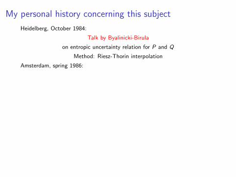
My personal history concerning this subject
Heidelberg, October 1984:
Talk by Byalinicki-Birula
on entropic uncertainty relation for P and Q
Method: Riesz-Thorin interpolation
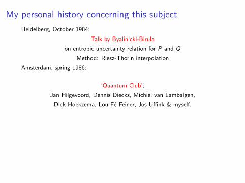
Amsterdam, spring 1986:
‘Quantum Club’:
Jan Hilgevoord, Dennis Diecks, Michiel van Lambalgen,
Dick Hoekzema, Lou-Fe Feiner, Jos Uffink & myself.
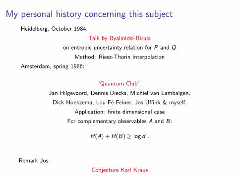
Application: finite dimensional case
For complementary observables A and B:
H(A) + H(B) ≥ log d .
Remark Jos:
Conjecture Karl Kraus

My personal history concerning this subject
Heidelberg, October 1984:
Talk by Byalinicki-Birula
on entropic uncertainty relation for P and Q
Method: Riesz-Thorin interpolation
Amsterdam, spring 1986:
‘Quantum Club’:
Jan Hilgevoord, Dennis Diecks, Michiel van Lambalgen,
Dick Hoekzema, Lou-Fe Feiner, Jos Uffink & myself.
Application: finite dimensional case
For complementary observables A and B:
H(A) + H(B) ≥ log d .
Remark Jos:
Conjecture Karl Kraus

1986:
Jos met Karl Kraus, mentioning that we had a proof.
Karl Kraus: “Publish!”
Sequel
We wrote down the result in a Phys. Rev. Letter. (1988)
(Impact factor 7.4.)
Jos elaborated the result in his Ph. D. thesis.
I published in Quantum Probability and Applications V (1990)
(Impact factor ε > 0.)
The Letter still is, for both of us, by far the most cited item on our publication
lists.
The inequality has been applied in quantum key distribution, entanglement
distillation, has been improved upon in special cases, and is generally
well-known in quantum information.

1986: Jos met Karl Kraus, mentioning that we had a proof.
Karl Kraus: “Publish!”
Sequel
We wrote down the result in a Phys. Rev. Letter. (1988)
(Impact factor 7.4.)
Jos elaborated the result in his Ph. D. thesis.
I published in Quantum Probability and Applications V (1990)
(Impact factor ε > 0.)
The Letter still is, for both of us, by far the most cited item on our publication
lists.
The inequality has been applied in quantum key distribution, entanglement
distillation, has been improved upon in special cases, and is generally
well-known in quantum information.

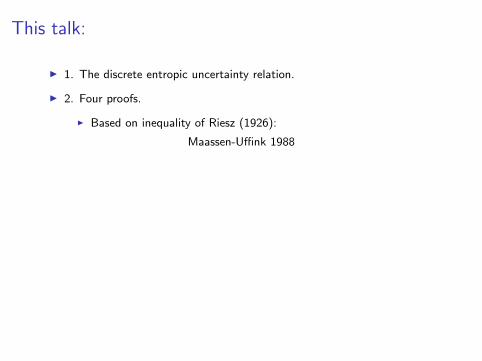
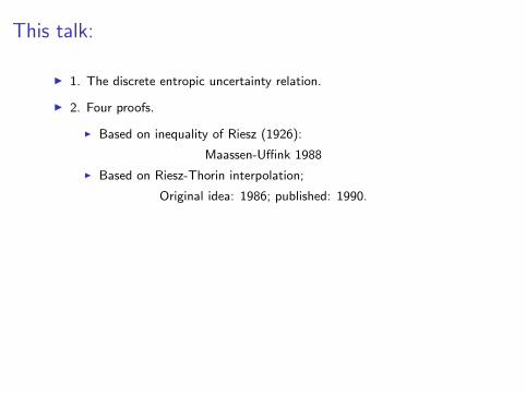
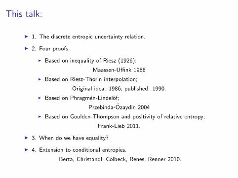
This talk:
I 1. The discrete entropic uncertainty relation.
I 2. Four proofs.
I Based on inequality of Riesz (1926):
Maassen-Uffink 1988
I Based on Riesz-Thorin interpolation;
Original idea: 1986; published: 1990.
I Based on Phragmen-Lindelof;
Przebinda-Ozaydin 2004
I Based on Goulden-Thompson and positivity of relative entropy;
Frank-Lieb 2011.
I 3. When do we have equality?
I 4. Extension to conditional entropies.
Berta, Christandl, Colbeck, Renes, Renner 2010.

What are we talking about?
H : complex Hilbert space of dimension d ;
ψ : unit vector in H .
Two orthonormal bases in H:
e1, e2, . . . , ed ; e1, e2, . . . , ed .
From the above we form:
Two probability distributions:
πj := |〈ej , ψ〉|2 ; πk := |〈ek , ψ〉|2 .
Largest scalar product:
c := maxi,j|〈ei , ej〉| .

The discrete entropic uncertainty relation
DefinitionThe entropy H(π) of a discrete probability distribution π = (π1, π2, . . . , πd) is
defined as
H(π) := −d∑
j=1
πj log πj .
This is the expected amount of information which the measurement will give, or
equivalently, the amount of uncertainty which we have before the measurement.
Theorem (1)
The sum of the two uncertainties satisfies:
H(π) + H(π) ≥ log1
c2.

Extreme cases:
I e1 = e1: Then c = 1 and the inequality becomes vacuous:
H(π) + H(π) ≥ 0 .
In fact, equality can be reached by putting ψ = e1 = e1.
Both outcomes are completely certain.
I Mutually Unbiased Bases:
|〈ej , ek〉|2 =1
d: c =
1√d.
Then we obtain Karl Kraus’s conjecture:
H(π) + H(π) ≥ log d .
Again equality can be reached by putting ψ = e1. Then π = δ1 and π is
the uniform distribution.
One outcome is certain, the other completely uncertain.

Extreme cases:
I e1 = e1:
Then c = 1 and the inequality becomes vacuous:
H(π) + H(π) ≥ 0 .
In fact, equality can be reached by putting ψ = e1 = e1.
Both outcomes are completely certain.
I Mutually Unbiased Bases:
|〈ej , ek〉|2 =1
d: c =
1√d.
Then we obtain Karl Kraus’s conjecture:
H(π) + H(π) ≥ log d .
Again equality can be reached by putting ψ = e1. Then π = δ1 and π is
the uniform distribution.
One outcome is certain, the other completely uncertain.

Extreme cases:
I e1 = e1: Then c = 1 and the inequality becomes vacuous:
H(π) + H(π) ≥ 0 .
In fact, equality can be reached by putting ψ = e1 = e1.
Both outcomes are completely certain.
I Mutually Unbiased Bases:
|〈ej , ek〉|2 =1
d: c =
1√d.
Then we obtain Karl Kraus’s conjecture:
H(π) + H(π) ≥ log d .
Again equality can be reached by putting ψ = e1. Then π = δ1 and π is
the uniform distribution.
One outcome is certain, the other completely uncertain.

Extreme cases:
I e1 = e1: Then c = 1 and the inequality becomes vacuous:
H(π) + H(π) ≥ 0 .
In fact, equality can be reached by putting ψ = e1 = e1.
Both outcomes are completely certain.
I Mutually Unbiased Bases:
|〈ej , ek〉|2 =1
d: c =
1√d.
Then we obtain Karl Kraus’s conjecture:
H(π) + H(π) ≥ log d .
Again equality can be reached by putting ψ = e1. Then π = δ1 and π is
the uniform distribution.
One outcome is certain, the other completely uncertain.

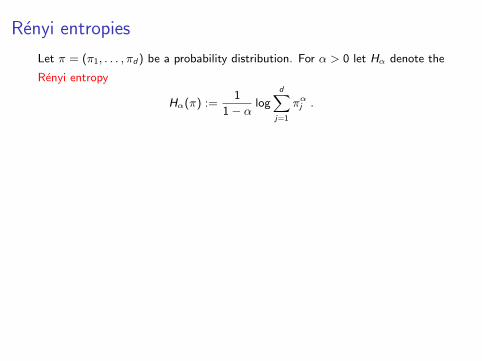
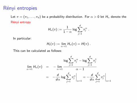
Renyi entropies
Let π = (π1, . . . , πd) be a probability distribution. For α > 0 let Hα denote the
Renyi entropy
Hα(π) :=1
1− α logd∑
j=1
παj .
In particular:
H1(π) := limα→1
Hα(π) = H(π) .
This can be calculated as follows:
limα→1
Hα(π) = − limα→1
logd∑
j=1
παj − logd∑
j=1
π1j
α− 1
= − d
dαlog
d∑j=1
παj
∣∣∣∣α=1
= − d
dα
d∑j=1
παj
∣∣∣∣α=1
= −d∑
j=1
πj log πj = H(π) .

Renyi entropies
Let π = (π1, . . . , πd) be a probability distribution. For α > 0 let Hα denote the
Renyi entropy
Hα(π) :=1
1− α logd∑
j=1
παj .
In particular:
H1(π) := limα→1
Hα(π) = H(π) .
This can be calculated as follows:
limα→1
Hα(π) =
− limα→1
logd∑
j=1
παj − logd∑
j=1
π1j
α− 1
= − d
dαlog
d∑j=1
παj
∣∣∣∣α=1
= − d
dα
d∑j=1
παj
∣∣∣∣α=1
= −d∑
j=1
πj log πj = H(π) .

Renyi entropies
Let π = (π1, . . . , πd) be a probability distribution. For α > 0 let Hα denote the
Renyi entropy
Hα(π) :=1
1− α logd∑
j=1
παj .
In particular:
H1(π) := limα→1
Hα(π) = H(π) .
This can be calculated as follows:
limα→1
Hα(π) = − limα→1
logd∑
j=1
παj − logd∑
j=1
π1j
α− 1
= − d
dαlog
d∑j=1
παj
∣∣∣∣α=1
= − d
dα
d∑j=1
παj
∣∣∣∣α=1
= −d∑
j=1
πj log πj = H(π) .

Renyi entropies
Let π = (π1, . . . , πd) be a probability distribution. For α > 0 let Hα denote the
Renyi entropy
Hα(π) :=1
1− α logd∑
j=1
παj .
In particular:
H1(π) := limα→1
Hα(π) = H(π) .
This can be calculated as follows:
limα→1
Hα(π) = − limα→1
logd∑
j=1
παj − logd∑
j=1
π1j
α− 1
= − d
dαlog
d∑j=1
παj
∣∣∣∣α=1
= − d
dα
d∑j=1
παj
∣∣∣∣α=1
= −d∑
j=1
πj log πj = H(π) .

Renyi entropies
Let π = (π1, . . . , πd) be a probability distribution. For α > 0 let Hα denote the
Renyi entropy
Hα(π) :=1
1− α logd∑
j=1
παj .
In particular:
H1(π) := limα→1
Hα(π) = H(π) .
This can be calculated as follows:
limα→1
Hα(π) = − limα→1
logd∑
j=1
παj − logd∑
j=1
π1j
α− 1
= − d
dαlog
d∑j=1
παj
∣∣∣∣α=1
= − d
dα
d∑j=1
παj
∣∣∣∣α=1
= −d∑
j=1
πj log πj
= H(π) .

Renyi entropies
Let π = (π1, . . . , πd) be a probability distribution. For α > 0 let Hα denote the
Renyi entropy
Hα(π) :=1
1− α logd∑
j=1
παj .
In particular:
H1(π) := limα→1
Hα(π) = H(π) .
This can be calculated as follows:
limα→1
Hα(π) = − limα→1
logd∑
j=1
παj − logd∑
j=1
π1j
α− 1
= − d
dαlog
d∑j=1
παj
∣∣∣∣α=1
= − d
dα
d∑j=1
παj
∣∣∣∣α=1
= −d∑
j=1
πj log πj = H(π) .

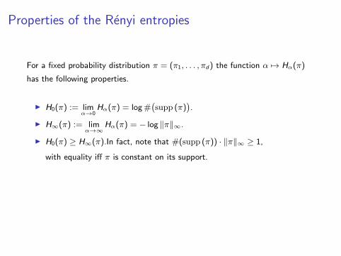
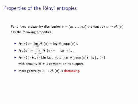
Properties of the Renyi entropies
For a fixed probability distribution π = (π1, . . . , πd) the function α 7→ Hα(π)
has the following properties.
I H0(π) := limα→0
Hα(π) = log #(supp (π)
).
I H∞(π) := limα→∞
Hα(π) = − log ‖π‖∞.
I H0(π) ≥ H∞(π).In fact, note that #(supp (π)) · ‖π‖∞ ≥ 1,
with equality iff π is constant on its support.
I More generally: α 7→ Hα(π) is decreasing.
In fact, the derivative has a meaning: it is −(1− α)−2 times the relative
entropy of the normalised power distribution πα with respect to π.

Properties of the Renyi entropies
For a fixed probability distribution π = (π1, . . . , πd) the function α 7→ Hα(π)
has the following properties.
I H0(π) := limα→0
Hα(π) = log #(supp (π)
).
I H∞(π) := limα→∞
Hα(π) = − log ‖π‖∞.
I H0(π) ≥ H∞(π).
In fact, note that #(supp (π)) · ‖π‖∞ ≥ 1,
with equality iff π is constant on its support.
I More generally: α 7→ Hα(π) is decreasing.
In fact, the derivative has a meaning: it is −(1− α)−2 times the relative
entropy of the normalised power distribution πα with respect to π.

Properties of the Renyi entropies
For a fixed probability distribution π = (π1, . . . , πd) the function α 7→ Hα(π)
has the following properties.
I H0(π) := limα→0
Hα(π) = log #(supp (π)
).
I H∞(π) := limα→∞
Hα(π) = − log ‖π‖∞.
I H0(π) ≥ H∞(π).In fact, note that #(supp (π)) · ‖π‖∞ ≥ 1,
with equality iff π is constant on its support.
I More generally: α 7→ Hα(π) is decreasing.
In fact, the derivative has a meaning: it is −(1− α)−2 times the relative
entropy of the normalised power distribution πα with respect to π.

Generalized entropic uncertainty relations
Actually in our 1988 Phys. Rev. Letter Jos proved the inequality for all the
Renyi entropies:
Theorem (2)
Let α, α ∈ [0,∞] be such that 1α
+ 1α
= 2. Then
Hα(π) + Hα(π) ≥ log1
c2.
Of course, taking α→ 1 we obtain the ordinary entropic uncertainty relation.
Also, since α 7→ Hα(π) is decreasing, we have for all α ≤ 1:
Hα(π) + Hα(π) ≥ log1
c2.

Generalized entropic uncertainty relations
Actually in our 1988 Phys. Rev. Letter Jos proved the inequality for all the
Renyi entropies:
Theorem (2)
Let α, α ∈ [0,∞] be such that 1α
+ 1α
= 2.
Then
Hα(π) + Hα(π) ≥ log1
c2.
Of course, taking α→ 1 we obtain the ordinary entropic uncertainty relation.
Also, since α 7→ Hα(π) is decreasing, we have for all α ≤ 1:
Hα(π) + Hα(π) ≥ log1
c2.

Generalized entropic uncertainty relations
Actually in our 1988 Phys. Rev. Letter Jos proved the inequality for all the
Renyi entropies:
Theorem (2)
Let α, α ∈ [0,∞] be such that 1α
+ 1α
= 2. Then
Hα(π) + Hα(π) ≥ log1
c2.
Of course, taking α→ 1 we obtain the ordinary entropic uncertainty relation.
Also, since α 7→ Hα(π) is decreasing, we have for all α ≤ 1:
Hα(π) + Hα(π) ≥ log1
c2.

Generalized entropic uncertainty relations
Actually in our 1988 Phys. Rev. Letter Jos proved the inequality for all the
Renyi entropies:
Theorem (2)
Let α, α ∈ [0,∞] be such that 1α
+ 1α
= 2. Then
Hα(π) + Hα(π) ≥ log1
c2.
Of course, taking α→ 1 we obtain the ordinary entropic uncertainty relation.
Also, since α 7→ Hα(π) is decreasing, we have for all α ≤ 1:
Hα(π) + Hα(π) ≥ log1
c2.

Notation
We shall indicate the components of ψ in the two bases by
ψk := 〈ek , ψ〉 ;
ψj := 〈ej , ψ〉 .
If we define the unitary matrix U = (ujk)dj,k=1 by
ujk := 〈ej , ek〉 ,
then we may write
ψj = 〈ej , ψ〉 =d∑
k=1
〈ej , ek〉〈ek , ψ〉 =d∑
k=1
ujkψk .
So our raw data are now a unitary d × d matrix U and a unit vector ψ ∈ Cn,
and we have ψ = Uψ.

Our 1988 proof
Theorem (Marcel Riesz 1928)
For 1 ≤ p ≤ 2 ≤ p ≤ ∞ with 1p
+ 1p
= 1:
(c
d∑j=1
|ψj |p)1/p
≤
(c
d∑j=1
|ψk |p)1/p
.
More briefly this can be stated as follows:
c1/p‖ψ‖p ≤ c1/p‖ψ‖p .
Equivalently:
log ‖ψ‖p − log ‖ψ‖p ≥(
1
p− 1
p
)log c .

Our 1988 proof
Theorem (Marcel Riesz 1928)
For 1 ≤ p ≤ 2 ≤ p ≤ ∞ with 1p
+ 1p
= 1:
(c
d∑j=1
|ψj |p)1/p
≤
(c
d∑j=1
|ψk |p)1/p
.
More briefly this can be stated as follows:
c1/p‖ψ‖p ≤ c1/p‖ψ‖p .
Equivalently:
log ‖ψ‖p − log ‖ψ‖p ≥(
1
p− 1
p
)log c .

Our 1988 proof
Theorem (Marcel Riesz 1928)
For 1 ≤ p ≤ 2 ≤ p ≤ ∞ with 1p
+ 1p
= 1:
(c
d∑j=1
|ψj |p)1/p
≤
(c
d∑j=1
|ψk |p)1/p
.
More briefly this can be stated as follows:
c1/p‖ψ‖p ≤ c1/p‖ψ‖p .
Equivalently:
log ‖ψ‖p − log ‖ψ‖p ≥(
1
p− 1
p
)log c .

Our 1988 proof
Theorem (Marcel Riesz 1928)
For 1 ≤ p ≤ 2 ≤ p ≤ ∞ with 1p
+ 1p
= 1:
(c
d∑j=1
|ψj |p)1/p
≤
(c
d∑j=1
|ψk |p)1/p
.
More briefly this can be stated as follows:
c1/p‖ψ‖p ≤ c1/p‖ψ‖p .
Equivalently:
log ‖ψ‖p − log ‖ψ‖p ≥(
1
p− 1
p
)log c .

Our 1988 proof
Theorem (Marcel Riesz 1928)
For 1 ≤ p ≤ 2 ≤ p ≤ ∞ with 1p
+ 1p
= 1:
(c
d∑j=1
|ψj |p)1/p
≤
(c
d∑j=1
|ψk |p)1/p
.
More briefly this can be stated as follows:
c1/p‖ψ‖p ≤ c1/p‖ψ‖p .
Equivalently:
log ‖ψ‖p − log ‖ψ‖p ≥(
1
p− 1
p
)log c .

Our 1988 proof
Theorem (Marcel Riesz 1928)
For 1 ≤ p ≤ 2 ≤ p ≤ ∞ with 1p
+ 1p
= 1:
(c
d∑j=1
|ψj |p)1/p
≤
(c
d∑j=1
|ψk |p)1/p
.
More briefly this can be stated as follows:
c1/p‖ψ‖p ≤ c1/p‖ψ‖p .
Equivalently:
log ‖ψ‖p − log ‖ψ‖p ≥(
1
p− 1
p
)log c .
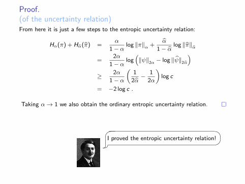
Proof.(of the uncertainty relation)
From here it is just a few steps to the entropic uncertainty relation:
Hα(π) + Hα(π) =α
1− α log ‖π‖α +α
1− α log ‖π‖α
=2α
1− α log(‖ψ‖2α − log ‖ψ‖2α
)≥ 2α
1− α
(1
2α− 1
2α
)log c
= −2 log c .
Taking α→ 1 we also obtain the ordinary entropic uncertainty relation.
� � ��I proved the entropic uncertainty relation!

Proof.(of the uncertainty relation)From here it is just a few steps to the entropic uncertainty relation:
Hα(π) + Hα(π) =
α
1− α log ‖π‖α +α
1− α log ‖π‖α
=2α
1− α log(‖ψ‖2α − log ‖ψ‖2α
)≥ 2α
1− α
(1
2α− 1
2α
)log c
= −2 log c .
Taking α→ 1 we also obtain the ordinary entropic uncertainty relation.
� � ��I proved the entropic uncertainty relation!

Proof.(of the uncertainty relation)From here it is just a few steps to the entropic uncertainty relation:
Hα(π) + Hα(π) =α
1− α log ‖π‖α +α
1− α log ‖π‖α
=2α
1− α log(‖ψ‖2α − log ‖ψ‖2α
)≥ 2α
1− α
(1
2α− 1
2α
)log c
= −2 log c .
Taking α→ 1 we also obtain the ordinary entropic uncertainty relation.
� � ��I proved the entropic uncertainty relation!

Proof.(of the uncertainty relation)From here it is just a few steps to the entropic uncertainty relation:
Hα(π) + Hα(π) =α
1− α log ‖π‖α +α
1− α log ‖π‖α
=2α
1− α log(‖ψ‖2α − log ‖ψ‖2α
)
≥ 2α
1− α
(1
2α− 1
2α
)log c
= −2 log c .
Taking α→ 1 we also obtain the ordinary entropic uncertainty relation.
� � ��I proved the entropic uncertainty relation!

Proof.(of the uncertainty relation)From here it is just a few steps to the entropic uncertainty relation:
Hα(π) + Hα(π) =α
1− α log ‖π‖α +α
1− α log ‖π‖α
=2α
1− α log(‖ψ‖2α − log ‖ψ‖2α
)≥ 2α
1− α
(1
2α− 1
2α
)log c
= −2 log c .
Taking α→ 1 we also obtain the ordinary entropic uncertainty relation.
� � ��I proved the entropic uncertainty relation!

Proof.(of the uncertainty relation)From here it is just a few steps to the entropic uncertainty relation:
Hα(π) + Hα(π) =α
1− α log ‖π‖α +α
1− α log ‖π‖α
=2α
1− α log(‖ψ‖2α − log ‖ψ‖2α
)≥ 2α
1− α
(1
2α− 1
2α
)log c
= −2 log c .
Taking α→ 1 we also obtain the ordinary entropic uncertainty relation.
� � ��I proved the entropic uncertainty relation!

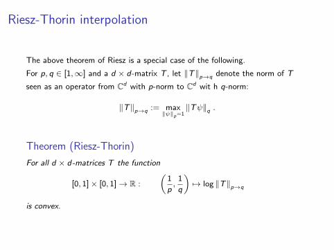
Riesz-Thorin interpolation
The above theorem of Riesz is a special case of the following.
For p, q ∈ [1,∞] and a d × d-matrix T , let ‖T‖p→q denote the norm of T
seen as an operator from Cd with p-norm to Cd wit h q-norm:
‖T‖p→q := max‖ψ‖p=1
‖Tψ‖q .
Theorem (Riesz-Thorin)
For all d × d-matrices T the function
[0, 1]× [0, 1]→ R :
(1
p,
1
q
)7→ log ‖T‖p→q
is convex.

Entropic uncertainty by interpolation
Let U be a unitary d × d-matrix, ψ ∈ Cd a vector of unit 2-norm: ‖ψ‖2 = 1,
and let c := maxj,k |〈ej , ek〉|. Then we have
‖U‖2→2 = 1 since U is unitary;
‖U‖1→∞ = c since |(Uψ)j | =
∣∣∣∣∣d∑
k=1
ujkψk
∣∣∣∣∣ ≤ cd∑
k=1
|ψk | .
According to the Riesz-Thorin interpolation theorem the function
fU : [0, 1]→ [0, 1] :1
p7→ log ‖U‖p→p
is convex.
Since fU(12
)= log ‖U‖2→2 = 0 and fU(1) = log ‖U‖1→∞ = log c, we conclude
that
f ′(
1
2
)≤
f (1)− f ( 12)
1− 12
≤ 2 log c .
Entropic uncertainty by interpolation
Let U be a unitary d × d-matrix, ψ ∈ Cd a vector of unit 2-norm: ‖ψ‖2 = 1,
and let c := maxj,k |〈ej , ek〉|.
Then we have
‖U‖2→2 = 1 since U is unitary;
‖U‖1→∞ = c since |(Uψ)j | =
∣∣∣∣∣d∑
k=1
ujkψk
∣∣∣∣∣ ≤ cd∑
k=1
|ψk | .
According to the Riesz-Thorin interpolation theorem the function
fU : [0, 1]→ [0, 1] :1
p7→ log ‖U‖p→p
is convex.
Since fU(12
)= log ‖U‖2→2 = 0 and fU(1) = log ‖U‖1→∞ = log c, we conclude
that
f ′(
1
2
)≤
f (1)− f ( 12)
1− 12
≤ 2 log c .

Entropic uncertainty by interpolation
Let U be a unitary d × d-matrix, ψ ∈ Cd a vector of unit 2-norm: ‖ψ‖2 = 1,
and let c := maxj,k |〈ej , ek〉|. Then we have
‖U‖2→2 = 1 since U is unitary;
‖U‖1→∞ = c since |(Uψ)j | =
∣∣∣∣∣d∑
k=1
ujkψk
∣∣∣∣∣ ≤ cd∑
k=1
|ψk | .
According to the Riesz-Thorin interpolation theorem the function
fU : [0, 1]→ [0, 1] :1
p7→ log ‖U‖p→p
is convex.
Since fU(12
)= log ‖U‖2→2 = 0 and fU(1) = log ‖U‖1→∞ = log c, we conclude
that
f ′(
1
2
)≤
f (1)− f ( 12)
1− 12
≤ 2 log c .

On the other hand, for all ψ ∈ Cd and p ∈ [0, ,∞]:
fU
(1
p
)= log ‖U‖p→p ≥ log ‖Uψ‖p − log ‖ψ‖p .
Since we have equality at 1p
= 12, we may differentiate the above inequality:
f ′U
(1
2
)≥ −H(|ψ|2)− H(|ψ|2) .
Since f ′U( 12) ≤ 2 log c, it follows that H(|ψ|2) + H(|ψ|2) ≥ log(1/c2).
On the other hand, for all ψ ∈ Cd and p ∈ [0, ,∞]:
fU
(1
p
)= log ‖U‖p→p ≥ log ‖Uψ‖p − log ‖ψ‖p .
Since we have equality at 1p
= 12, we may differentiate the above inequality:
f ′U
(1
2
)≥ −H(|ψ|2)− H(|ψ|2) .
Since f ′U( 12) ≤ 2 log c, it follows that H(|ψ|2) + H(|ψ|2) ≥ log(1/c2).

On the other hand, for all ψ ∈ Cd and p ∈ [0, ,∞]:
fU
(1
p
)= log ‖U‖p→p ≥ log ‖Uψ‖p − log ‖ψ‖p .
Since we have equality at 1p
= 12, we may differentiate the above inequality:
f ′U
(1
2
)≥ −H(|ψ|2)− H(|ψ|2) .
Since f ′U( 12) ≤ 2 log c, it follows that H(|ψ|2) + H(|ψ|2) ≥ log(1/c2).

On the other hand, for all ψ ∈ Cd and p ∈ [0, ,∞]:
fU
(1
p
)= log ‖U‖p→p ≥ log ‖Uψ‖p − log ‖ψ‖p .
Since we have equality at 1p
= 12, we may differentiate the above inequality:
f ′U
(1
2
)≥ −H(|ψ|2)− H(|ψ|2) .
Since f ′U( 12) ≤ 2 log c, it follows that H(|ψ|2) + H(|ψ|2) ≥ log(1/c2).

On the other hand, for all ψ ∈ Cd and p ∈ [0, ,∞]:
fU
(1
p
)= log ‖U‖p→p ≥ log ‖Uψ‖p − log ‖ψ‖p .
Since we have equality at 1p
= 12, we may differentiate the above inequality:
f ′U
(1
2
)≥ −H(|ψ|2)− H(|ψ|2) .
Since f ′U( 12) ≤ 2 log c, it follows that H(|ψ|2) + H(|ψ|2) ≥ log(1/c2).

On the other hand, for all ψ ∈ Cd and p ∈ [0, ,∞]:
fU
(1
p
)= log ‖U‖p→p ≥ log ‖Uψ‖p − log ‖ψ‖p .
Since we have equality at 1p
= 12, we may differentiate the above inequality:
f ′U
(1
2
)≥ −H(|ψ|2)− H(|ψ|2) .
Since f ′U( 12) ≤ 2 log c, it follows that H(|ψ|2) + H(|ψ|2) ≥ log(1/c2).

Riesz convexity and functions on the strip.
The source of the Riesz-Thorin convexity result, the secret weapon of Riesz’
brilliant student Thorin, is the study of analytic functions on a strip in the
complex plane. We now give a direct proof of the entropic uncertainty relation
using this secret weapon.
It starts from the following result in function theory.
Let S denote the strip { z ∈ C | 0 ≤ Re z ≤ 1 }.
Theorem (Phragmen-Lindelof)
Let F be a bounded holomorphic function on S such that |F (z)| ≤ 1 on the
boundary of S. Then |F (z)| ≤ 1 on all of S.

Riesz convexity and functions on the strip.
The source of the Riesz-Thorin convexity result, the secret weapon of Riesz’
brilliant student Thorin, is the study of analytic functions on a strip in the
complex plane.
We now give a direct proof of the entropic uncertainty relation
using this secret weapon.
It starts from the following result in function theory.
Let S denote the strip { z ∈ C | 0 ≤ Re z ≤ 1 }.
Theorem (Phragmen-Lindelof)
Let F be a bounded holomorphic function on S such that |F (z)| ≤ 1 on the
boundary of S. Then |F (z)| ≤ 1 on all of S.

Riesz convexity and functions on the strip.
The source of the Riesz-Thorin convexity result, the secret weapon of Riesz’
brilliant student Thorin, is the study of analytic functions on a strip in the
complex plane. We now give a direct proof of the entropic uncertainty relation
using this secret weapon.
It starts from the following result in function theory.
Let S denote the strip { z ∈ C | 0 ≤ Re z ≤ 1 }.
Theorem (Phragmen-Lindelof)
Let F be a bounded holomorphic function on S such that |F (z)| ≤ 1 on the
boundary of S. Then |F (z)| ≤ 1 on all of S.

Riesz convexity and functions on the strip.
The source of the Riesz-Thorin convexity result, the secret weapon of Riesz’
brilliant student Thorin, is the study of analytic functions on a strip in the
complex plane. We now give a direct proof of the entropic uncertainty relation
using this secret weapon.
It starts from the following result in function theory.
Let S denote the strip { z ∈ C | 0 ≤ Re z ≤ 1 }.
Theorem (Phragmen-Lindelof)
Let F be a bounded holomorphic function on S such that |F (z)| ≤ 1 on the
boundary of S.
Then |F (z)| ≤ 1 on all of S.

Riesz convexity and functions on the strip.
The source of the Riesz-Thorin convexity result, the secret weapon of Riesz’
brilliant student Thorin, is the study of analytic functions on a strip in the
complex plane. We now give a direct proof of the entropic uncertainty relation
using this secret weapon.
It starts from the following result in function theory.
Let S denote the strip { z ∈ C | 0 ≤ Re z ≤ 1 }.
Theorem (Phragmen-Lindelof)
Let F be a bounded holomorphic function on S such that |F (z)| ≤ 1 on the
boundary of S. Then |F (z)| ≤ 1 on all of S.

Thorin’s MAGIC FUNCT ION
F (z) := c−zd∑
j=1
d∑k=1
ψj |ψj |z · ujk · ψk |ψk |z .
I F is bounded: |F (z)| ≤ c−1∑jk |ψj | · |ψk | = c−1‖ψ‖1 · ‖ψ‖1.
I F (0) = 1: F (0) = 〈ψ,Uψ〉 = ‖ψ‖2
2 = 1.
I |F (iy)| ≤ 1: F (iy) = c−iy 〈ϕ,Uχ〉,
where ϕj := |ψj |iy ψj and χk := |ψk |iyψk are unit vectors;
I |F (1 + iy)| ≤ 1: |F (1 + iy)| ≤ 1c
∑jk |ψj |2 · |ujk | · |ψk |2.
It follows that |F (z)| ≤ 1 for all z ∈ S . In particular: ReF ′(0) ≤ 0, but. . .
F ′(0) = − log c −d∑
j=1
log |ψj |ψj(Uψ)j −d∑
k=1
log |ψk |(U∗ψ)kψk
= − log c − 1
2
(H(|ψ|2 + H(|ψ|2)
).
The statement follows.

The theorem of Frank and Lieb
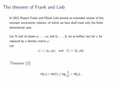
In 2011 Rupert Frank and Elliott Lieb proved an extended version of the
entropic uncertainty relation, of which we here shall treat only the finite
dimensional case.
Let H and its bases e1, . . . , ed and e1, . . . , ed be as before, but let ψ be
replaced by a density matrix ρ.
Let
πj := 〈ej , ρej〉 and πj := 〈ej , ρej〉
Theorem (3)
H(π) + H(π) ≥ log1
c2+ H(ρ) ,
where H(ρ) is the von Neumann entropy of ρ.

The theorem of Frank and Lieb
In 2011 Rupert Frank and Elliott Lieb proved an extended version of the
entropic uncertainty relation, of which we here shall treat only the finite
dimensional case.
Let H and its bases e1, . . . , ed and e1, . . . , ed be as before, but let ψ be
replaced by a density matrix ρ.
Let
πj := 〈ej , ρej〉 and πj := 〈ej , ρej〉
Theorem (3)
H(π) + H(π) ≥ log1
c2+ H(ρ) ,
where H(ρ) is the von Neumann entropy of ρ.

The proof by Frank and Lieb
The proof is based on two pillars of quantum information theory:
Lemma (positivity of relative entropy)
For all pairs of density matrices ρ, σ we have
tr ρ log σ ≤ tr ρ log ρ .
Lemma (Golden-Thompson inequality)
For all self-adjoint d × d-matrices A and B we have
tr(
eA+B)≤ tr
(eAeB
).

The proof by Frank and Lieb
Fix a state ρ and define negative definite matrices A and A by
A :=d∑
i=1
log πi |ei 〉〈ei | and A :=d∑
i=1
log πi |ei 〉〈ei | .
Let σ be the ’Gibbs state’ σ :=eA+A
tr eA+A.
Then we have
H(π) + H(π) = −tr ρ(A + A)
= −tr ρ log σ − log tr(eA+A)
≥ −tr ρ log ρ− log tr(eAeA)
But the trace in the last term can be written as
tr(
eAeA)
=d∑
i,j=1
πi πjtr(|ei 〉〈ei |ej〉〈ej |
)=
d∑i,j=1
πi πj |uij |2 ≤ c2 .
The statement follows.

The proof by Frank and LiebFix a state ρ and define negative definite matrices A and A by
A :=d∑
i=1
log πi |ei 〉〈ei | and A :=d∑
i=1
log πi |ei 〉〈ei | .
Let σ be the ’Gibbs state’ σ :=eA+A
tr eA+A.
Then we have
H(π) + H(π) = −tr ρ(A + A)
= −tr ρ log σ − log tr(eA+A)
≥ −tr ρ log ρ− log tr(eAeA)
But the trace in the last term can be written as
tr(
eAeA)
=d∑
i,j=1
πi πjtr(|ei 〉〈ei |ej〉〈ej |
)
=d∑
i,j=1
πi πj |uij |2 ≤ c2 .
The statement follows.
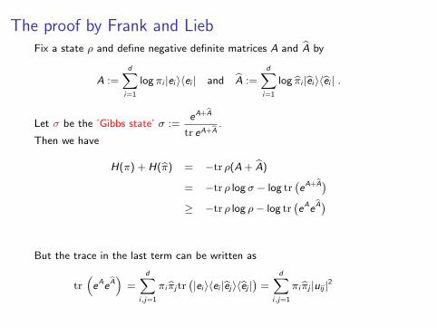
The proof by Frank and LiebFix a state ρ and define negative definite matrices A and A by
A :=d∑
i=1
log πi |ei 〉〈ei | and A :=d∑
i=1
log πi |ei 〉〈ei | .
Let σ be the ’Gibbs state’ σ :=eA+A
tr eA+A.
Then we have
H(π) + H(π) = −tr ρ(A + A)
= −tr ρ log σ − log tr(eA+A)
≥ −tr ρ log ρ− log tr(eAeA)
But the trace in the last term can be written as
tr(
eAeA)
=d∑
i,j=1
πi πjtr(|ei 〉〈ei |ej〉〈ej |
)=
d∑i,j=1
πi πj |uij |2
≤ c2 .
The statement follows.
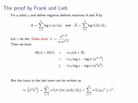
The proof by Frank and LiebFix a state ρ and define negative definite matrices A and A by
A :=d∑
i=1
log πi |ei 〉〈ei | and A :=d∑
i=1
log πi |ei 〉〈ei | .
Let σ be the ’Gibbs state’ σ :=eA+A
tr eA+A.
Then we have
H(π) + H(π) = −tr ρ(A + A)
= −tr ρ log σ − log tr(eA+A)
≥ −tr ρ log ρ− log tr(eAeA)
But the trace in the last term can be written as
tr(
eAeA)
=d∑
i,j=1
πi πjtr(|ei 〉〈ei |ej〉〈ej |
)=
d∑i,j=1
πi πj |uij |2 ≤ c2 .
The statement follows.

The proof by Frank and LiebFix a state ρ and define negative definite matrices A and A by
A :=d∑
i=1
log πi |ei 〉〈ei | and A :=d∑
i=1
log πi |ei 〉〈ei | .
Let σ be the ’Gibbs state’ σ :=eA+A
tr eA+A.
Then we have
H(π) + H(π) = −tr ρ(A + A)
= −tr ρ log σ − log tr(eA+A)
≥ −tr ρ log ρ− log tr(eAeA)
But the trace in the last term can be written as
tr(
eAeA)
=d∑
i,j=1
πi πjtr(|ei 〉〈ei |ej〉〈ej |
)=
d∑i,j=1
πi πj |uij |2 ≤ c2 .
The statement follows.

When is de inequality sharp?
The ’magic function’ lends itself most easily to spotting equality in the
uncertainty relation.
We can have H(π) + H(π) = log(1/c2), (which means that F ′(0) = 0),
only if
F (z) = 1 everywhere on the strip!
(This is Hopf’s theorem.)
From this we deduce:
TheoremWe have equality in the discrete entropic uncertainty relation if and only if π
and π are constant on their supports, say D and D respectively, and moreover:
#D ·#D =1
c2.
In particular, #D ·#D ≤ d :the supports are small!

When is de inequality sharp?
The ’magic function’ lends itself most easily to spotting equality in the
uncertainty relation.
We can have H(π) + H(π) = log(1/c2), (which means that F ′(0) = 0),
only if
F (z) = 1 everywhere on the strip!
(This is Hopf’s theorem.)
From this we deduce:
Theorem
We have equality in the discrete entropic uncertainty relation if and only if π
and π are constant on their supports, say D and D respectively, and moreover:
#D ·#D =1
c2.
In particular, #D ·#D ≤ d :the supports are small!

When is de inequality sharp?
The ’magic function’ lends itself most easily to spotting equality in the
uncertainty relation.
We can have H(π) + H(π) = log(1/c2), (which means that F ′(0) = 0),
only if
F (z) = 1 everywhere on the strip!
(This is Hopf’s theorem.)
From this we deduce:
TheoremWe have equality in the discrete entropic uncertainty relation if and only if π
and π are constant on their supports, say D and D respectively, and moreover:
#D ·#D =1
c2.
In particular, #D ·#D ≤ d :the supports are small!

When is de inequality sharp?
The ’magic function’ lends itself most easily to spotting equality in the
uncertainty relation.
We can have H(π) + H(π) = log(1/c2), (which means that F ′(0) = 0),
only if
F (z) = 1 everywhere on the strip!
(This is Hopf’s theorem.)
From this we deduce:
TheoremWe have equality in the discrete entropic uncertainty relation if and only if π
and π are constant on their supports, say D and D respectively, and moreover:
#D ·#D =1
c2.
In particular, #D ·#D ≤ d :
the supports are small!

When is de inequality sharp?
The ’magic function’ lends itself most easily to spotting equality in the
uncertainty relation.
We can have H(π) + H(π) = log(1/c2), (which means that F ′(0) = 0),
only if
F (z) = 1 everywhere on the strip!
(This is Hopf’s theorem.)
From this we deduce:
TheoremWe have equality in the discrete entropic uncertainty relation if and only if π
and π are constant on their supports, say D and D respectively, and moreover:
#D ·#D =1
c2.
In particular, #D ·#D ≤ d :the supports are small!

Examples of saturation
I Suppose d = nn, and we have conjugate bases: 〈ej , ek〉 =1√d
e2πid
jk .
Then we can take the pure state vector given by
ψk =1√n
if k is divisible by n; 0 otherwise;
ψj =1√n
if j is divisible by n; 0 otherwise.
II But there are many others examples.
For instance
U =
1√2
12
12
1√2− 1
2− 1
2
0 1√2− 1√
2
; ψ =
1
0
0
; ψ =1√2
1
1
0
.

Proof of saturation theorem
Sufficiency:
H(π) + H(π) = log(#D) + log(#D) = log(#D ·#D) = log 1c2
.
Necessity:
F ′(0) = 0 implies F (z) = 1 for all z ∈ S :
c−z∑j,k
ψj |ψj |z ujk ψk |ψk |z = 1 .
In particular for z = 1, writing ψk = |ψk | · e iθk and the same for ψ:∑j,k
|ψj |2 · |ψk |2 ·(
e−i θj · e iθk · 1
cujk
)︸ ︷︷ ︸
=1!
= 1 .
Let D, D denote the supports of ψ and ψ. Then we have for j ∈ D, k ∈ D:
ujk = c · e i(θj−θk ) .
Hence for j ∈ D: ψj =∑k∈D
ujkψk = ce i θj∑k∈D
e−iθkψk = ce i θj∑k
|ψk |.
So |ψ| is constant on its support.
The same holds for ψ.

Proof of saturation theoremSufficiency:
H(π) + H(π) = log(#D) + log(#D) = log(#D ·#D) = log 1c2
.
Necessity:
F ′(0) = 0 implies F (z) = 1 for all z ∈ S :
c−z∑j,k
ψj |ψj |z ujk ψk |ψk |z = 1 .
In particular for z = 1, writing ψk = |ψk | · e iθk and the same for ψ:
∑j,k
|ψj |2 · |ψk |2 ·(
e−i θj · e iθk · 1
cujk
)︸ ︷︷ ︸
=1!
= 1 .
Let D, D denote the supports of ψ and ψ. Then we have for j ∈ D, k ∈ D:
ujk = c · e i(θj−θk ) .
Hence for j ∈ D: ψj =∑k∈D
ujkψk = ce i θj∑k∈D
e−iθkψk = ce i θj∑k
|ψk |.
So |ψ| is constant on its support.
The same holds for ψ.

Proof of saturation theoremSufficiency:
H(π) + H(π) = log(#D) + log(#D) = log(#D ·#D) = log 1c2
.
Necessity:
F ′(0) = 0 implies F (z) = 1 for all z ∈ S :
c−z∑j,k
ψj |ψj |z ujk ψk |ψk |z = 1 .
In particular for z = 1, writing ψk = |ψk | · e iθk and the same for ψ:∑j,k
|ψj |2 · |ψk |2 ·(
e−i θj · e iθk · 1
cujk
)︸ ︷︷ ︸
=1!
= 1 .
Let D, D denote the supports of ψ and ψ. Then we have for j ∈ D, k ∈ D:
ujk = c · e i(θj−θk ) .
Hence for j ∈ D: ψj =∑k∈D
ujkψk = ce i θj∑k∈D
e−iθkψk = ce i θj∑k
|ψk |.
So |ψ| is constant on its support.
The same holds for ψ.

Proof of saturation theoremSufficiency:
H(π) + H(π) = log(#D) + log(#D) = log(#D ·#D) = log 1c2
.
Necessity:
F ′(0) = 0 implies F (z) = 1 for all z ∈ S :
c−z∑j,k
ψj |ψj |z ujk ψk |ψk |z = 1 .
In particular for z = 1, writing ψk = |ψk | · e iθk and the same for ψ:∑j,k
|ψj |2 · |ψk |2 ·(
e−i θj · e iθk · 1
cujk
)︸ ︷︷ ︸
=1!
= 1 .
Let D, D denote the supports of ψ and ψ.
Then we have for j ∈ D, k ∈ D:
ujk = c · e i(θj−θk ) .
Hence for j ∈ D: ψj =∑k∈D
ujkψk = ce i θj∑k∈D
e−iθkψk = ce i θj∑k
|ψk |.
So |ψ| is constant on its support.
The same holds for ψ.
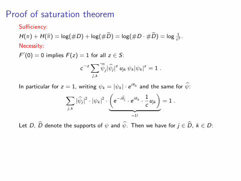
Proof of saturation theoremSufficiency:
H(π) + H(π) = log(#D) + log(#D) = log(#D ·#D) = log 1c2
.
Necessity:
F ′(0) = 0 implies F (z) = 1 for all z ∈ S :
c−z∑j,k
ψj |ψj |z ujk ψk |ψk |z = 1 .
In particular for z = 1, writing ψk = |ψk | · e iθk and the same for ψ:∑j,k
|ψj |2 · |ψk |2 ·(
e−i θj · e iθk · 1
cujk
)︸ ︷︷ ︸
=1!
= 1 .
Let D, D denote the supports of ψ and ψ. Then we have for j ∈ D, k ∈ D:
ujk = c · e i(θj−θk ) .
Hence for j ∈ D: ψj =∑k∈D
ujkψk = ce i θj∑k∈D
e−iθkψk = ce i θj∑k
|ψk |.
So |ψ| is constant on its support.
The same holds for ψ.
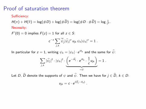
Proof of saturation theoremSufficiency:
H(π) + H(π) = log(#D) + log(#D) = log(#D ·#D) = log 1c2
.
Necessity:
F ′(0) = 0 implies F (z) = 1 for all z ∈ S :
c−z∑j,k
ψj |ψj |z ujk ψk |ψk |z = 1 .
In particular for z = 1, writing ψk = |ψk | · e iθk and the same for ψ:∑j,k
|ψj |2 · |ψk |2 ·(
e−i θj · e iθk · 1
cujk
)︸ ︷︷ ︸
=1!
= 1 .
Let D, D denote the supports of ψ and ψ. Then we have for j ∈ D, k ∈ D:
ujk = c · e i(θj−θk ) .
Hence for j ∈ D:
ψj =∑k∈D
ujkψk = ce i θj∑k∈D
e−iθkψk = ce i θj∑k
|ψk |.
So |ψ| is constant on its support.
The same holds for ψ.

Proof of saturation theoremSufficiency:
H(π) + H(π) = log(#D) + log(#D) = log(#D ·#D) = log 1c2
.
Necessity:
F ′(0) = 0 implies F (z) = 1 for all z ∈ S :
c−z∑j,k
ψj |ψj |z ujk ψk |ψk |z = 1 .
In particular for z = 1, writing ψk = |ψk | · e iθk and the same for ψ:∑j,k
|ψj |2 · |ψk |2 ·(
e−i θj · e iθk · 1
cujk
)︸ ︷︷ ︸
=1!
= 1 .
Let D, D denote the supports of ψ and ψ. Then we have for j ∈ D, k ∈ D:
ujk = c · e i(θj−θk ) .
Hence for j ∈ D: ψj =∑k∈D
ujkψk = ce i θj∑k∈D
e−iθkψk = ce i θj∑k
|ψk |.
So |ψ| is constant on its support.
The same holds for ψ.

Proof of saturation theoremSufficiency:
H(π) + H(π) = log(#D) + log(#D) = log(#D ·#D) = log 1c2
.
Necessity:
F ′(0) = 0 implies F (z) = 1 for all z ∈ S :
c−z∑j,k
ψj |ψj |z ujk ψk |ψk |z = 1 .
In particular for z = 1, writing ψk = |ψk | · e iθk and the same for ψ:∑j,k
|ψj |2 · |ψk |2 ·(
e−i θj · e iθk · 1
cujk
)︸ ︷︷ ︸
=1!
= 1 .
Let D, D denote the supports of ψ and ψ. Then we have for j ∈ D, k ∈ D:
ujk = c · e i(θj−θk ) .
Hence for j ∈ D: ψj =∑k∈D
ujkψk = ce i θj∑k∈D
e−iθkψk = ce i θj∑k
|ψk |.
So |ψ| is constant on its support.
The same holds for ψ.

Entropies and algebras
In 2010 Berta, Christandl, Colbeck, Renes, and Renner proved an uncertainty
relation concerning conditional entropies.
For a clean formulation I think it is profitable to use the language of *-algebras.
If (X , µ) is a probability space, then the entropy H(α) of a finite partition α of
X is
H(α) := −∑A∈α
µ(A) logµ(A) .
This translates to a finite abelian subalgebra C of L∞(X , µ) as follows:
Hϕ(C) := sup {−k∑
i=1
ϕ(pi ) logϕ(pi ) | p1, . . . , pk partition of unity in C } .
And then to general finite-dimensional *-algebras as follows:
Hϕ(A) := inf {Hϕ(C) | C ⊂ A maximal abelian } .

Entropies and algebras
In 2010 Berta, Christandl, Colbeck, Renes, and Renner proved an uncertainty
relation concerning conditional entropies.
For a clean formulation I think it is profitable to use the language of *-algebras.
If (X , µ) is a probability space, then the entropy H(α) of a finite partition α of
X is
H(α) := −∑A∈α
µ(A) log µ(A) .
This translates to a finite abelian subalgebra C of L∞(X , µ) as follows:
Hϕ(C) := sup {−k∑
i=1
ϕ(pi ) logϕ(pi ) | p1, . . . , pk partition of unity in C } .
And then to general finite-dimensional *-algebras as follows:
Hϕ(A) := inf {Hϕ(C) | C ⊂ A maximal abelian } .

Conditional entropies and algebras
Let A and B be finite dimensional *-subalgebras of Mn, and let ϕ be a state on
Mn.
We define
Hϕ(A|B) := Hϕ(A ∨ B)− Hϕ(B) .
Horodecki 1996:Negative conditional entropies can occur in case of
entanglement.
Example:
A = Mn ⊗ 1l, B := 1l⊗Mn, and ϕ(x) := 〈ψ, xψ〉 for ψ = 1√n
∑ni=1 |ei 〉〈ei |.
then
Hϕ(A ∨ B) = Hϕ(Mn ⊗Mn) = 0
and
Hϕ(B) = log n .
The difference being
Hϕ(A|B) = − log n .

Conditional entropies and algebrasLet A and B be finite dimensional *-subalgebras of Mn, and let ϕ be a state on
Mn.
We define
Hϕ(A|B) := Hϕ(A ∨ B)− Hϕ(B) .
Horodecki 1996:Negative conditional entropies can occur in case of
entanglement.
Example:
A = Mn ⊗ 1l, B := 1l⊗Mn, and ϕ(x) := 〈ψ, xψ〉 for ψ = 1√n
∑ni=1 |ei 〉〈ei |.
then
Hϕ(A ∨ B) = Hϕ(Mn ⊗Mn) = 0
and
Hϕ(B) = log n .
The difference being
Hϕ(A|B) = − log n .

Conditional entropies and algebrasLet A and B be finite dimensional *-subalgebras of Mn, and let ϕ be a state on
Mn.
We define
Hϕ(A|B) := Hϕ(A ∨ B)− Hϕ(B) .
Horodecki 1996:
Negative conditional entropies can occur in case of
entanglement.
Example:
A = Mn ⊗ 1l, B := 1l⊗Mn, and ϕ(x) := 〈ψ, xψ〉 for ψ = 1√n
∑ni=1 |ei 〉〈ei |.
then
Hϕ(A ∨ B) = Hϕ(Mn ⊗Mn) = 0
and
Hϕ(B) = log n .
The difference being
Hϕ(A|B) = − log n .

Conditional entropies and algebrasLet A and B be finite dimensional *-subalgebras of Mn, and let ϕ be a state on
Mn.
We define
Hϕ(A|B) := Hϕ(A ∨ B)− Hϕ(B) .
Horodecki 1996:Negative conditional entropies can occur in case of
entanglement.
Example:
A = Mn ⊗ 1l, B := 1l⊗Mn, and ϕ(x) := 〈ψ, xψ〉 for ψ = 1√n
∑ni=1 |ei 〉〈ei |.
then
Hϕ(A ∨ B) = Hϕ(Mn ⊗Mn) = 0
and
Hϕ(B) = log n .
The difference being
Hϕ(A|B) = − log n .

Conditional entropies and algebrasLet A and B be finite dimensional *-subalgebras of Mn, and let ϕ be a state on
Mn.
We define
Hϕ(A|B) := Hϕ(A ∨ B)− Hϕ(B) .
Horodecki 1996:Negative conditional entropies can occur in case of
entanglement.
Example:
A = Mn ⊗ 1l, B := 1l⊗Mn, and ϕ(x) := 〈ψ, xψ〉 for ψ = 1√n
∑ni=1 |ei 〉〈ei |.
then
Hϕ(A ∨ B) = Hϕ(Mn ⊗Mn) = 0
and
Hϕ(B) = log n .
The difference being
Hϕ(A|B) = − log n .

A conditional entropic uncertainty relation
Theorem (Berta et al. 2010)
Let A := Mn ⊗ 1l and B := 1l⊗Mm.
Let C and C be maximal abelian subalgebras of A.
Then for all states ρ on Mn ⊗Mm:
Hρ(C|B) + Hρ(C|B) ≥ log1
c2+ Hρ(A|B) .

A conditional entropic uncertainty relation
Theorem (Berta et al. 2010)
Let A := Mn ⊗ 1l and B := 1l⊗Mm.
Let C and C be maximal abelian subalgebras of A.
Then for all states ρ on Mn ⊗Mm:
Hρ(C|B) + Hρ(C|B) ≥ log1
c2+ Hρ(A|B) .

A conditional entropic uncertainty relation
Theorem (Berta et al. 2010)
Let A := Mn ⊗ 1l and B := 1l⊗Mm.
Let C and C be maximal abelian subalgebras of A.
Then for all states ρ on Mn ⊗Mm:
Hρ(C|B) + Hρ(C|B) ≥ log1
c2+ Hρ(A|B) .

A conditional entropic uncertainty relation
Theorem (Berta et al. 2010)
Let A := Mn ⊗ 1l and B := 1l⊗Mm.
Let C and C be maximal abelian subalgebras of A.
Then for all states ρ on Mn ⊗Mm:
Hρ(C|B) + Hρ(C|B) ≥ log1
c2+ Hρ(A|B) .

A conditional entropic uncertainty relation
Theorem (Berta et al. 2010)
Let A := Mn ⊗ 1l and B := 1l⊗Mm.
Let C and C be maximal abelian subalgebras of A.
Then for all states ρ on Mn ⊗Mm:
Hρ(C|B) + Hρ(C|B) ≥ log1
c2+ Hρ(A|B) .

A conditional entropic uncertainty relation
Theorem (Berta et al. 2010)
Let A := Mn ⊗ 1l and B := 1l⊗Mm.
Let C and C be maximal abelian subalgebras of A.
Then for all states ρ on Mn ⊗Mm:
Hρ(C|B) + Hρ(C|B) ≥ log1
c2+ Hρ(A|B) .