- 1 -

Estimation of genomic characteristics by analyzing k-mer frequency in de novo genome projects

Binghang Liu1,2

*, Yujian Shi1*, Jianying Yuan

1*, Xuesong Hu

1,3, Hao Zhang

1,

Nan Li1, Zhenyu Li

1, Yanxiang Chen

1, Desheng Mu

1, Wei Fan

1,3*

1BGI-Shenzhen, Shenzhen, 518083, China.

2HKU-BGI Bioinformatics Algorithms and Core Technology Research Laboratory,

Hong Kong

3Biodynamic Optical Imaging Center, Peking University, Beijing 100871, China.

*Correspondence should be addressed to:

Binghang Liu: liubinghang@genomics.cn

Yujian Shi: shiyujian@genomics.cn

Jianying Yuan: yuanjianying@genomics.cn

Wei Fan: fanweisz09@gmail.com

Abstract

Background: With the fast development of next generation sequencing technologies, increasing

numbers of genomes are being de novo sequenced and assembled. However, most are in

fragmental and incomplete draft status, and thus it is often difficult to know the accurate genome

size and repeat content. Furthermore, many genomes are highly repetitive or heterozygous, posing

problems to current assemblers utilizing short reads. Therefore, it is necessary to develop efficient

assembly-independent methods for accurate estimation of these genomic characteristics.

Results: Here we present a framework for modeling the distribution of k-mer frequency from

sequencing data and estimating the genomic characteristics such as genome size, repeat structure

and heterozygous rate. By introducing novel techniques of k-mer individuals, float precision

estimation, and proper treatment of sequencing error and coverage bias, the estimation accuracy of

our method is significantly improved over existing methods. We also studied how the various

- 2 -

genomic and sequencing characteristics affect the estimation accuracy using simulated sequencing

data, and discussed the limitations on applying our method to real sequencing data.

Conclusion: Based on this research, we show that the k-mer frequency analysis can be used as a

general and assembly-independent method for estimating genomic characteristics, which can

improve our understanding of a species genome, help design the sequencing strategy of genome

projects, and guide the development of assembly algorithms. The programs developed in this

research are written using C/C++ and freely accessible at ftp://ftp.genomics.org.cn/pub/gce.

Keywords

K-mer, genome size, repeat, heterozygous, estimation, Poisson, Bayesian

Background

In recent years, more and more large genomes have been assembled by Whole-Genome-Shotgun

(WGS) short reads generated from next generation sequencing (NGS) technologies [1], including

the panda [2], potato[3], and many others. Many genomes are highly repetitive [4] or polyploid [5],

and some species have highly heterozygous diploid genomes [6]. These genomic characteristics

will increase the difficulty of the assembly processes, resulting in incomplete and fragmental

assembled sequences [7, 8], making it impossible to infer the accurate genome size and repeat

content only based on these assembled sequences. Another issue is that when genomes have an

extremely-high repeat content or heterozygous rate or are polyploid, the assembled sequences

using current available algorithms and short reads may become too fragmental and even unusable,

and so it is very important to get an accurate estimation of genomic characteristics before deciding

whether or not to start large-scale genome sequencing project.

Several experimental technologies have been developed to explore these genomic characteristics.

Feulgen densitometry and flow cytometry are the two most popular techniques used to estimate

the genome size, which is presented as the C-value [9]. DNA reassociation kinetics, also known

as C0t analysis, is usually used to measure and classify the repetitive DNA sequences in a genome

[10]. Some previous studies have performed estimation of heterozygosity using molecular markers

[11] or DNA microarrays [12], however, the performance of these techniques is often poor.

In de novo genome projects, analyzing the k-mer frequency, which is independent of genome

assembly, is widely used as an alternative way to estimate the genome size [2, 3, 13, 14]. However,

most projects have adopted a very rough estimation method (denoted below as “integer precision

estimation”), and their estimations are often not so accurate. The group of Michael S. Waterman

was the first to perform systematic study on the estimation of genome size and repeat structure

using k-mer frequency, and in 2003 they published a basic estimation method using the Mixed-

- 3 -

Poisson Model and EM algorithm [15]. Built on theoretically perfect data, their method has many

limitations, and the authors did not provide a usable tool for real application. In 2009, Shan &

Zheng extended the Michael S. Waterman’s method, and published a more generally applicable

software for genome size prediction (GSP) using the Bayesian estimation (BE) and EM iteration

[16]. GSP was initially developed for perfect data, and then adopts a simple approach to tolerate

some sequencing errors. Due to the quite complex characteristics of real sequencing data and the

immature status of the two methods, neither of them has been widely adopted by real applications

till now. Besides from them, we can’t find other more formal publications on this issue. In fact, it

is still very difficult for non-bioinformaticians to estimate the genomic characteristics properly.

In this article, we developed a more sophisticated method to satisfy the demands of real

applications. We improved the estimation accuracy over existing methods by introducing the k-

mer individuals and float precision estimation technique, and our method fully considers

sequencing characteristics such as error and coverage bias and has integrated a module for

processing them in order to get the best estimation of genomic characteristics. Futhermore, we

extend the previous application of estimating genome size and repeat structure to heterozygous

rate estimation. We also studied how the various genomic and sequencing characteristics affect the

estimation accuracy with simulated data, and demonstrated the application potential and

limitations of our model using real sequencing data from several finished genome projects. We

hope this work can help more genome projects to estimate the genomic characteristics more

accurately, and thus assist the understanding of their genome biology. We also suggest that future

genome projects, for which these genomic characteristics are not clear and may potentially pose

serious problems in assembly, to initially perform some small-scale sequencing (5~25X) and

estimate the genomic characteristics by k-mer frequency, which can then help determine the best

large-scale sequencing strategies and most suitable assembly algorithms.

Methods

Counting k-mer frequency

The counting of k-mer frequency in the sequencing data can be carried out using many of the

currently available tools, such as Meryl [17], Tallymer [18], and jellyfish [19], here we use our in-

house software Kmerfreq. Note that before counting, k-mer size (K) needs to be determined. K

should be kept small to prevent the overuse of computer memory, while still large enough so that

most k-mers are unique in the genome. Once K is determined, the maximum number of k-mers is

fixed as 4K. More detailed methods are shown in Supplemental materials.

Estimating sequencing depth and genome size

As an easy-to-understand illustrative example, we will first discuss the simplest k-mer frequency

(depth) model using hypothetical “ideal” reference genome and sequencing data. To start with, we

- 4 -

have to introduce two concepts: genomic frequency and coverage depth, which are used to refer to

the k-mer frequency counted from reference genome and sequencing data respectively. The

“ideal” reference genome here is assumed to be a random sequence, with no heterozygosity and no

repeats for a certain k-mer size, meaning the genomic frequency for all of these k-mers is 1. The

“ideal” sequencing data here is assumed to be produced from randomly single-ended and equal-

length whole genome shotgun process [20] without any sequencing errors or coverage bias, such

data meaning that the distribution for the start positions of reads follows a Poisson distribution.

When the read length (L) is far shorter than the genome size (L<<G), the bases and k-mers can be

also thought to be generated by random processes and their coverage depth will also follow

Poisson distributions [15, 21] (Figure 1a). Based on Poisson theory as well as the relationship

between base number and k-mer number, the sequencing depth (expected base coverage depth)

and genome size can be calculated by formulas (1) and (2) shown below[15], both of which are

important parameters for de novo projects.

Let nbase, nk-mer be the total number of bases and k-mers from sequencing data, and cbase, ck-mer be

the expected coverage depth for bases and k-mers, then we can get cbase = nbase / G and ck-mer = nk-

mer / G. As one read with length L generates L－K+1 k-mers, nk-mer / nbase = (L－K+1) / L. Thus:

- / ( 1)base k merc c L L K (1)

/ /k mer k mer base baseG n c n c (2)

Note: Formula (1) and (2) were firstly deduced by Michael S. Waterman’s group [15], and we list

them here to help understanding of the bellowing formulas. For simplification, in the following

parts of this paper, we will exclusively use c to represent ck-mer, and n to represent nk-mer.

Given that the read length (L) and k-mer size (K) are fixed values, to accurately estimate the

sequencing depth and genome size using the above formulas (1) and (2), we must firstly determine

two parameters: the total number of k-mers (n) and the expected k-mer coverage depth (c). The n

parameter can be directly obtained from the k-mer counting results. The parameter c is the key

parameter to be estimated in this part [15, 16], and it can be inferred from the widely adopted

Poisson distribution of k-mer frequency, denoted here as the k-mer species curve (Figure 1a),

represented in formula (3), which fits well-known Waterman’s estimation method [15]. Here we

also introduce another equivalent curve, the k-mer individuals curve (Figure 1a), represented in

formula (4). The number of k-mer individuals is the product of k-mer species number and

corresponding depth value. The points on these two types of k-mer coverage depth curves indicate

the ratio of k-mer species or individuals classified by each k-mer depth value respectively.From

observation on Figure 1a and deduction in formula (4), we found that the k-mer individuals curve

is a variation of Poisson distribution (denoted as varied-Poisson), which has the same figure shape

but moves rightwards wholly by one unit. In practice, we can use either of these two curves to

estimate the c value, or combine the results from each curve to make more solid estimation. The

- 5 -

two basic models shown in formulas (3) and (4) were denoted as the “basic model” in this paper.

Probability density function of k-mer species curve for the “ideal” genome:

( )!

xc

Kspecies

cP x e

x

(3)

Probability density function of k-mer individuals curve for the “ideal” genome:

( ) ( ) / ( 1)Kindividuals Kspecies KspeciesP x xP x c P x (4)

Note: Formula (3) was first introduced by Michael S. Waterman’s group [15], while formula (4)

was introduced by us for the first time. x in the two probability density functions, refer to the k-

mer coverage depth.

After we obtained one of the two k-mer coverage depth curves, a quick and rough way is to use

the observed peak depth value as the estimated c, which is an integer value. This method is

denoted as integer precision estimation here, which has been widely adopted by previous and

current genome projects. However, in most cases, the real c value is not an integer (Figure 1b). To

estimate c more accurately with float precision, we developed a new algorithm by using the

relationships between the neighboring points in the k-mer coverage depth distribution curve,

denoted as float precision estimation here, shown as the formulas (5) and (6). The detailed

deductions are shown in Supplemental materials.

Formulas to calculate c with float precision:

( 1)

( 1)( )

Kspecies

Kspecies

P xc x

P x

(5)

( 1)

( )

Kindividuals

Kindividuals

P xc x

P x

(6)

Note: Theoretically, x is arbitrary, and a pair of neighboring points is enough for estimation of c.

However, to estimate c more accurately, it is better to calculate c independently using 5 to 10 pairs

of points adjacent to the depth peak and adopt the average, to our experience.

Exploring repetitive genomes

We used the “ideal” genome to introduce the basic model above, but real genomes often contain

differing amounts of repeat sequences [22], which bring great challenges to the assembly

processes [23]. In this section, we will use the human reference genome and the “ideal”

sequencing data simulated from it as an example to explore the relationship between k-mers and

repeats.

The k-mers localized in repeat regions will not appear uniquely in the genome, and their genomic

frequencies are in line with the copy number of the repeats. We firstly counted the genomic k-mer

- 6 -

(K=17) frequency in the human reference genome. Then k-mers were classified by each genomic

frequency (i), and the ratio of k-mer species (ai) and individuals (bi) for each class were calculated

(Figure 2a). We also plotted the k-mer species and individuals curves from the simulated

sequencing data shown in Figure 2b. Repeats in the genome will cause several peaks on both the

k-mer species and individuals curves, the heights of which are closely related to the ai and bi

values respectively in Figure 2a. The k-mer species curve for repetitive genome had previously

been modeled as a compound of discrete Poisson distributions [15], shown in formula (7), each of

which was generated by a class of k-mers with specific genomic frequency (i) and expected

coverage depth (ci) [15]. We showed that the k-mer individuals curve in Figure 2b can also be

modeled as a compound of discrete varied-Poisson distributions in similar way, shown in formula

(8). Note that these two models are denoted as the “standard model” in this paper.

Assuming the range of genomic k-mer frequency is [1,m], ai=ni,genomic,Kspecies/ngenomic,Kspecies and

bi=ni,genomic,Kindividuals/ngenomic,Kindividuals are the ratios of k-mer species and individuals with genomic

frequency i, and ci=i×c is the expected coverage depth of k-mers with genomic frequency

i ,where c is the expected coverage depth of unique k-mers (genomic frequency i=1). Then we can

get:

Probability density function of k-mer species curve for repetitive genome:

,1

( ) ( )m

Kspecies i Kspecies iiP x a P x

(7)

Probability density function of k-mer individuals curve for repetitive genome:

,1( ) ( )

m

Kindividuals i Kindividuals iiP x b P x

(8)

Note: PKspecies,i(x) means Poisson distribution with expected coverage depth ci, PKindividuals,i(x)

means varied-Poisson distribution with expected coverage depth ci.

Formula (7) was first introduced by Michael S. Waterman’s group [15], we listed it here for

comparison with formula (8).

Both of the ai and bi values can reflect the repeat structure in genome, though they have slightly

different meaning. For simplification, we only use ai to describe repeats, because ai and bi values

can be converted to each other. To estimate the ai values for de novo projects where a reference

genome does not exist, the Waterman [15] and Shan [16] groups have provided alternative EM

approaches based on Bayes models, in which each k-mer species has two attributes: the genomic

frequency and the coverage depth. Firstly, the experience-based or equal prior probability values

are assigned to all the genomic k-mer frequencies, and then the posterior probability values for

these genomic k-mer frequencies are calculated using formula (9) shown below. Next, the

resulting posterior probability values are used as the input prior probability and this process is

iterated until the input prior and resulting posterior probabilities are merged. During these iteration

cycles, the ci values are also adjusted to be more accurate.

- 7 -

Here we used a similar method to Waterman [15] and Shan [16]groups for ai estimation, but a

different method for c estimation, shown in formula (10) . Essentially, this method is equivalent to

applying our float precision estimation method shown in formula (5) on the part of genomic

unique k-mers (genomic frequency == one). These genomic unique k-mers are obtained by

removing the contributions of repeat sequences (genomic frequency >= 2) on the major peak

region of the k-mer species curve, with the help of estimated ai values whose accuracy are

improved along with the Bayes iteration cycles. Here the major peak should be formed by the

genomic unique k-mers. If the difference between the major and minor peaks is not significant,

larger k-mer size should be used, shown in Figure 2cd. Based on the compound Poisson model,

we found that the genome size can be calculated by the total k-mer number (nk-mer) and the

expected coverage depth of unique k-mers (c): G = nk-mer / c. Using the iterated re-calculated more

accurate c, we can estimate genome size with higher accuracy. More detailed deductions are

shown in Supplemental materials

In the Bayes model, we define:

ai: the ratio (probability) of k-mer species with genomic frequency i, i=1,2,….,m.

vj: the ratio (probability) of k-mer species with coverage depth j, j=0, 1, 2, …,w.

c: the expected coverage depth for unique k-mer class with genomic frequency of one.

The prior probabilities:

( )( ) , ( | )

!

j ic

i

ic eP i a P j i

j

1 1

( | )( ) ( | )( | )

( ) ( | ) ( | )

i

m m

ii i

a P j iP i P j iP i j

P i P j i a P j i

The posterior probabilities: 0

( | )w

i jja P i j v

Therefore giving the iteration formula:

,

, 1

0 ,1

( | )

( | )

wi t

i t jmj i ti

a P j ia v

a P j i

(9)

,1, 1

1

,1, 1

( 1)( 1)

( )

Kspecies t

t

Kspecies t

P xc x

P x

(10)

Note: P(i) is the probability of one k-mer species with genomic frequency i. P(j|i) is the

probability of one k-mer species with genomic frequency i to be covered j times in sequencing

data. Although it is not possible to count v0, which would be the ratio of no covered k-mer species,

we can calculate it by v0=∑ai×PKspecies,i(0), where t refer to the iteration cycles. The c value is re-

calculated by the float precision estimation method using the major peak formed by unique k-mer

class with a genomic frequency of one. As the estimation of ai gets more accurate, the c value will

- 8 -

also become more accurate.

Exploring the heterozygous genomes

Besides repeats, most diploid genomes are heterozygous to a different degree, and most current de

bruijn graph (DBG) based assemblers cannot easily handle NGS short reads derived from highly

heterozygous genomes. It is very useful to estimate the heterozygous rate in the early stage of a

genome project. The Waterman and Shan groups have not addressed the issue of heterozygous rate

estimation.

To simplify things, the heterozygosity discussed in this paper is restricted to SNPs. We firstly

simulated SNP sites randomly in the “ideal” reference genome (haploid) to create “ideal”

heterozygous genome (diploid) and simulated “ideal” sequencing data from it. Then the k-mers

can be divided into 2 classes: the heterozygous k-mers and homozygous k-mers, which are

generated by the heterozygous and homozygous genomic regions respectively. It is supposed that

when the heterozygous rate is relatively low, the SNP sites will be distributed sparsely in the

whole genome, so there will be ideally 2 ×K heterozygous k-mers around each SNP site. These

heterozygous k-mers have half of the expected coverage depth and cause a new peak at 1/2

expected coverage depth in both the k-mer species and k-mer individuals curves shown in Figure

3ab. In order to be consistent, the k-mer genomic frequency for heterozygous genome here is

counted using the two haploid genomes and then dividing them by 2, then for the “ideal”

heterozygous genome here, there are only two genomic frequency values 1/2 and 1, and the

heterozygous rate can be roughly estimated with a1/2 using formula(11).

For heterozygous repetitive genome, the number of k-mer genomic frequency values will be

doubled compared to non-heterozygous repetitive genome, so there will also be 1.5, 2, 2.5, 3, etc.

The k-mer species and individuals curves for repetitive genomes (human) with various

heterozygous rate are shown in Figure 3cd. Theoretically, the number of peaks will also be

doubled compared to non-heterozygous repetitive genome. We extend the standard model

mentioned above to model heterozygosity, shown in formulas (12) and (13), and denoted as the

“heterozygous model”. In this model, there is no change in the formulas to estimate c and G, as

well as the Bayes model to estimate the ai values except for the step of i ,which changes from

integers to half of the integers for diploid genomes.

Because c should be estimated from the major peak generated by genomic homozygous unique k-

mers, the key problem for genome size estimation of heterozygous genome is to distinguish the

peaks on k-mer species or individuals curve. In practice, we can determine the homozygous

unique peak with the aids of some biological information or the rough assembly result. Though the

heterozygous rate for non-repetitive genome can be estimated by formula (11), it cannot be

extended to repetitive genome, because that there is no clear relationship between the a1/2 and

- 9 -

heterozygous rate here. More detailed methods are shown in Supplemental materials.

Formulas for heterozygous genomes:

1/2 1/2

1/2 1/2

/ (2 )

/ 2 (2 )

Kspecies

Kspecies Kspecies

a n K a

n a n K a

(11)

( 1/2)

,1/2( ) ( )

m step

Kspecies i Kspecies iiP x a P x

(12)

( 1/2)

,1/2( ) ( )

m step

Kindividuals i Kindividuals iiP x b P x

(13)

Dealing with sequencing error and coverage bias

The current real sequencing data usually have sequencing error and coverage bias problems, and

so the k-mer species or individuals curve reflects both the genomic and sequencing characteristics,

the mixture of which makes it difficult to estimate each type of characteristics accurately. Shan’s

group [16] has adopted a simple method to process sequencing errors, but neither Waterman’s nor

Shan’s groups has addressed the coverage bias problems. In the following, we will show how

sequencing error and coverage bias can affect the k-mer species and individuals curves, and point

out methods to deal with each of them in order to improve the estimation of genomic

characteristics.

Previous studies have demonstrated the k-mer distribution characteristics caused by sequencing

errors [16, 19]. To be more clear, here we illustrated this problem on Figure 4abc. Sequencing

error will generate a sharp left-side peak on the k-mer species curve (Figure 4a). As the rate of

sequencing errors increases, the left-side peak becomes larger, meanwhile, other normal peaks in

the curve would become smaller and also moves leftwards (Figure 4bc). Most of erroneous k-

mers caused by sequencing error are non-genomic k-mers, which appear in very low frequency

and form the left-side sharp peak. The frequency of the left erroneous k-mers, which have the

same sequence with the genomic k-mers, will be merged with the correct k-mers. Then it is

impossible to distinguish them just by frequency (Figure 4a).

As the distribution of erroneous k-mer is so complex, in practice, we use a simple method to deal

with sequencing error adapted from that of Shan’s group [16]. They just exclude the low depth k-

mers in the left-side sharp peak with a threshold at the lowest turning point (Figure 4a), and take

the left high depth k-mers as correct k-mers, which are used for estimating the c and ai values.

Using this method, most of the erroneous k-mers have been removed, but certain number of

correct k-mers will also be removed (Figure 4a), which will reduce the estimation accuracy. In

our method, we additionally use the estimated c and ai values to rebuild the theoretic distribution

curve, and compare it with the real distribution curve to adjust the number of correct k-mers.

- 10 -

Coverage bias [24-26] is a more complex issue than sequencing error, and there is few

publications discussed its affection on k-mer distribution characteristics. By analyzing genomic

data from the deadly 2011 German E. coli 0104:H4 outbreak [27], we found that there may be

many other factors besides GC content that can contribute to the coverage bias (Figure 4d).

Coverage bias will flatten the k-mer species or individuals curve, making it more difficult to

observe the peak depth clearly and estimate c accurately. Because of coverage bias, the

probabilities of sampling k-mers in the same genomic frequency class are not equal but appear in a

continuous spectrum, so the standard and heterozygous models with discrete Poisson distributions

need further development. This problem has not been previously considered in the published

models. Here we use an extended form with continuous Poisson or varied-Poisson distributions to

model the k-mer distribution with coverage bias, as shown in formulas (14) and (15), and denoted

as the “continuous model”. In theory, i~

does not mean genomic frequency any more, and so a~

i~ does

not reflect ratio of genomic frequency either, but it is related to the sampling probabilities of k-

mers in the sequencing data.

As a practical step, we used dense ranks of i~

with either a fixed equal step or dynamic non-equal

step to simulate the continuous model. If we set a fixed equal step of i~

, such as 1/4, 1/8, 1/16, the

continuous model is just a further extension of the heterozygous model in which the step of i is 1/2.

Here we suggest using the dynamic non-equal step model, which has advantage in both accuracy

and convenience, as shown in formulas (16) and (17). In this model, we use character “k” to

replace “i~

” because of the dynamic non-equal step. The estimation of a~

k in the Bayes iteration is

similar with that of fixed equal step models such as the standard and heterozygous models, but the

estimation of c~

k is different, as shown in formulas (18) and (19) respectively. Based on our

experiences demonstrated in Supplemental materials, we take the c~

k with the highest a~

k value as

the c value, which was used to estimate the genome size. Although it is difficult to infer genomic

ai values from the estimated a~

k values, we can sum up the multiple a~

k values around each peak to

roughly reflect each genomic ai values, especially for a1.

Probability function for k-mer species and individuals curves with coverage bias:

,

( ) ( )Kspecies i Kspecies iP x a P x di (14)

,

( ) ( )Kindividuals i Kindividuals iP x b P x di (15)

Implementing this, we used dense ranks with dynamic non-equal steps to simulate the continuous

model:

,1( ) ( )

m

Kspecies k Kspecies kkP x a P x

(16)

- 11 -

,1

( ) ( )m

Kindividuals k Kindividuals kkP x b P x

(17)

Note: m′ is the total number of Poisson distributions considered. The symbol k here stands for the

order, and there is no relation between k and c~

k.

The formulas in Bayes iterations for this dense discrete model:

( | )!

kcj

kc eP j k

j

,

, 1

0 ,1

( | )

( | )

wk t

k t jmj k tk

a P j ka v

a P j k

(18)

, 1

, 1

0, 1 , 11

( | )1

( | )

wk t

k t jmjk t k tk

a P j kc v

a a P j k

(19)

Note: the formula to calculate c~

k here is similar to that of the Waterman group.

Results and discussion

Relationship between data coverage and estimation accuracy

In this section, we investigate how data coverage affects the accuracy of genome size estimation.

To simplify matters, we will still use the “ideal” reference genome and simulated sequencing data

as an example. We evaluated the accuracy of estimation using the ratio between deviation size and

real genome size (ΔG/G). The ΔG/G values calculated by the 4 different methods (k-mer species

and individuals, together with integer precision estimation and float precision estimation) with

various expected k-mer coverage depth were plotted in Figure 5, and detailed methods to calculate

ΔG/G values are shown in Supplemental materials. The two integer precision ways give similar

results, ranging from 0.1%-10%; whist the two float precision ways also show similar results,

ranging from 0.01%-0.1%. When the expected k-mer coverage depth (ck-mer) is lower than 20,

there is a roughly two orders of magnitude difference between the integer precision and float

precision methods; when ck-mer is higher than 20 but lower than 85, there is still roughly a one

order of magnitude difference, which illustrate the significant advantage for the float precision

estimations over the integer precision estimations, especially when the ck-mer is relatively low. It

should be noted that the ΔG/G values from integer precision methods appear in periodic character,

and in particular the estimated genome size is almost always larger than the real value. In contrast,

the ΔG/G values from float precision ways are randomly distributed, i.e. no systematic bias, which

indicates the potential of getting the accurate estimation by averaging the results from multiple

experiments.

Estimating with various types of simulated data

In order to evaluate the performance of our models and analyze the influence of repeat content,

- 12 -

heterozygous rate, sequencing error and k-mer size on the accuracy of genomic characteristics

estimation, we simulated 48 sets of 25X coverage data from 4 species (E. coli, Arabidopsis,

Human, and Maize, the reference genome versions are shown in Table 1), with 4 ranks of

heterozygous rates (0%, 0.01%, 0.1%, 1%) and in combination with 3 ranks of sequencing error

rate (0%, 0.05%, 1%). As the sequencing coverage bias is too complex to model and simulate, it

was not considered in this section. For each data set, we calculated the 17-mer and 25-mer ai

values from the reference genomes. The reference genome sizes and some major ai values are

shown in Table 1, and the complete information of ai can be found in Table S1. The k-mer species

and individuals curves were plotted for each data set, and are shown in Figure S1.

To estimate the genome size and ai values from the simulated sequencing data, we applied the

heterozygous model to data sets with a heterozygous rate equal or larger than 0.1% and the

standard model to the other data sets, due to the fact that the heterozygous model is not

particularly sensitive with extreme-low heterozygous rate. We used ΔG/G to evaluate the accuracy

of genome size estimation. The distribution of ΔG/G values for maize is shown in Figure 6ab, and

those for other species can be found in Figure S2. Within these simulated data sets, about 15%,

73% and 95% of the ΔG/G values are smaller than 0.1%, 1%, and 5% respectively. For simplicity,

we used Δa1/a1 to evaluate the accuracy of ai estimation, and the distributions of Δa1/a1 values for

all species are shown in Figure S3. Similarly to the accuracy level of ΔG/G values, about 13%,

54%, and 92% of the Δa1/a1 values are smaller than 0.1%, 1%, and 5% respectively. With the

estimated c and ai values, we also calculated the estimated k-mer species and individuals curves

using the compound Poisson models, as shown in Figure S1, which are well consistent with their

theoretical curves, indicating the high accuracy of c and ai estimation.

For genome size estimation, we found that higher rates of repeats, heterozygosity and sequencing

error would result in lower accuracy, especially when the 3 factors occur together (Figure 6ab,

Figure S2 and Figure S4). Among these factors, sequencing error is the most difficult factor to deal

with, with the repeat and heterozygosity levels enhancing this effect. Besides these issues, the k-

mer size also influences the estimation accuracy. By comparing ΔG/G values from 17-mer and 25-

mer (as shown in Figure 6ab, Figure S5), we suggest using smaller k-mer size for data with high

heterozygosity and sequencing error rates. The evaluation of ai estimation and the analysis of

influencing factors are more complex than that of genome size, so it is difficult to get a clear

understanding of these. Additional results and discussion relating to this are shown in

Supplemental materials.

For repeat structure estimation, we additionally analyzed the non-heterozygous data for the four

species using the standard model and k-mer sizes ranging from 11 to 31, as the absolute ai values

are closely related with the k-mer sizes. Although in theory all the ai and bi values can be

- 13 -

calculated, in practice, we are usually only interested in a1 and b1, which related to the ratio of

unique k-mer species in the genome and the ratio of the genome covered by unique k-mers

respectively. Both the theoretical and estimated a1 (b1) values with various k-mer sizes are shown

in Figure 6cd, and are consistent with each other, indicating a very high accuracy of estimation. As

most short read assemblers have adopted the De Bruijn Graph algorithm, obtaining the a1 and b1

values with various k-mer sizes from the raw sequencing data, will be quite helpful for deciding

the suitable k-mer size in de novo assembly [28].

For heterozygosity estimation, we show all the estimated a1/2 values using the heterozygous

model and the inferred heterozygous rates by formula (11) in Table S2. We found that the order of

magnitude of estimated heterozygous rate is in accordance with that of heterozygous rate we

simulated, except for extremely low-heterozygous rates (nearly homozygosis). The estimation

accuracy is affected by the repeat content and sequencing error rate, especially when the theoretic

heterozygous rate is very low.

Analyzing real sequencing data from de novo genome projects

In this section, we evaluated the performance of our models on real sequencing data from 5

finished de novo genome projects, including E. coli-O104:H4 [27], the Leaf-cutting ant [14],

Potato [3], Panda[2], and YH genome (human diploid reference genome from an anonymous

Asian individual) [28, 29]. The repeat content of these genomes is different, and they are nearly

homozygous except the panda and YH genomes with a roughly 0.1% heterozygous rate. As the

sequencing error rate for real data is usually high and difficult to estimate, on top of counting all k-

mers from the raw data, we also adopted two alternative ways to pre-process sequencing error. The

first is by ignoring the low quality k-mers in the step of counting k-mer frequency, detailed

methods of which can be found in Supplemental materials. The other method is running an error

correction tool [28, 30] on the raw reads and then counting k-mer frequency on the error corrected

sequencing data.

To estimate the genomic characteristics from these sequencing data, all of which have coverage

bias problem, we adopted 3 alternative methods: (1) Rough estimation of genome size, by

observing the integer c from the major peak depth and excluding k-mers with depth lower than the

lowest-point threshold to obtain the correct k-mer number. (2) Application of the standard model,

the float-point c and ai values can be estimated. As the estimated distribution curve differs greatly

with that of real data (Figure 7a), we use the same approach in method (1) to estimate correct k-

mer number. (3) Application of the continuous model, the float-point c and ai values can be

estimated, and the estimated distribution curve is well consistent with that of real data (Figure 7b),

and we used it to adjust the correct k-mer number. The estimated genome size values for each data

set with each method are shown in Table 2, and the estimated information relating to the ai values

can be found in Table S3 and Table S4. Moreover, all the real and estimated k-mer species and

- 14 -

individuals curves are shown in Figure S6.

Taking the reported genome sizes in the published papers as reference, we found that over 80% of

the ΔG/G or Δa1/a1 values from all the used methods are smaller than 5%, indicating the high

estimation accuracy and application potential for real sequencing data. The estimated genome

sizes from error corrected data tends to be smaller than that of all raw and low-quality filtered data,

which can be explained as that the current error correction tool takes some of the low-frequency k-

mer species as erroneous k-mers and removes them in the error corrected data. In contrast, there is

no obvious difference between the estimated G values from low-quality filtered data and all raw

data, indicating that there is no severe systematical bias in the k-mer filtering process. The

estimated genome sizes from the rough estimation tend to be larger than that estimated by standard

and continuous models, which may be caused by the low-accurate integer c estimation and the

erroneous k-mers. In contrast, there is no obvious difference between the estimated G values from

the standard and continuous models, indicating that both methods can be used to estimate the

genome size with real sequencing data. Although the standard model is not suitable for data with

coverage bias, the peak depth of unique k-mers is almost unchanged, and this model can

automatically summarize the effects around each genomic ai and so it generates similar result to

the continuous model. However, there is no obvious trend in the influence of a1 estimation

accuracy for either the error processing methods or the estimation models. Additional results and

discussions relating to this are shown in Supplemental materials. As the real reference G and ai

values are unknown and the results from different methods fluctuate, it is not easy to determine

which method is better, and we feel that further investigation is needed to improve the estimation

accuracy with real sequencing data.

To have a clear view of the repeat structure in these genomes as well as choosing suitable k-mer

size for the De Brujin Graph assembly, we further estimated the a1(b1) values with various k-mer

sizes by the continuous model, shown in Figure 7cd. The estimated a1(b1) values for smaller k-mer

sizes are nearly consistent with the reference values calculated from assembled genomes, but those

for larger k-mer sizes become lower than reference values, which may be related to the increasing

number and non-uniform distribution of erroneous k-mers. Moreover, the published reference

genomes may still be lacking some repeat sequences, resulting in higher reference a1(b1) values.

Although the estimation accuracy is not as high as that of simulated data, the trend is still correct,

and the results can be used to guide de novo assembly. Conversely, it is almost impossible to

estimate the heterozygous rate for these low heterozygous genomes because of the sequencing

coverage bias, which hides the effect of heterozygosity, indicating that the real application of

heterozygous rate estimation is limited only to highly heterozygous genomes.

- 15 -

Comparison with previously published tools

Finally, we compared the performance of our program with published related applications. The

Waterman program [15] requires the preparation of input data in a specific format, and this

program is only written for testing their model and is unable to be used in practical application, so

was not included for comparison. The Shan groups program (GSP)[16] has been designed to

predict the genome size using k-mer frequency derived from NGS data, which takes similar input

as our program (GCE), so it is convenient for comparisons. To compare the estimation accuracy

between these two programs, we simulated two sets of sequencing data from the E. coli,

Arabidopsis, Human and Maize reference genomes, one set containing no sequencing error, with

the other set with a 1% sequencing error, and both without heterozygosity, because GSP was not

designed for heterozygous rate estimation (although it may have the ability to tolerate some low

level of heterozygosity).

The accuracy of estimated genome size and a1 using the two programs GCE and GSP are shown in

Table 3. Overall, GCE has a significant higher estimation accuracy over GSP, especially on large

and repetitive genomes. Considering on the error-free data first (Table 3a), GSP generates similar

results with GCE for relatively repeat-less genomes (E. coli and Arabidopsis), but generates a

poorer result for repetitive genomes (Human and Maize) in comparison to GCE. The explanation

for this is likely due to the difference of ci re-calculation method in the iteration cycles between

GSP and GCE.. GCE focused on the unique k-mers (a1), minimized the affection of repeat k-mers

and improved estimation accuracy even for the repeat abundant genomes.

We then compared the estimation accuracy using data with 1% sequencing error (Table 3b). The

estimation accuracy of genome size and a1 in GCE are both a little lower than that on error-free

data. In contrast, the genome size estimation in GSP seems a little better than its error-free results,

which may be explained by the fact that GSP tends to generate smaller predictions but sequencing

error will make these predictions larger. Notably, the a1 in GSP is worse even for relatively repeat-

less genomes. To make a more in-depth investigation, we ran GSP and GCE on the data sets with

various combinations of sequencing errors, heterozygous rate, and k-mer sizes, and show the

results in Table S5.

Conclusion

In this article, we have introduced a methodological framework for genomic characteristics

analysis based on raw sequencing data, which can estimate genome size, repeat structure and

heterozygous rate of the sequenced sample. This is likely not limited solely to these characteristics,

and other genomic characteristics such as polyploidy and DNA contamination are also likely to be

estimated. The k-mer frequency curves also provide comprehensive information about the

- 16 -

sequencing characteristics, such as error rate and degree of coverage bias. The proper processing

of these issues will be important for the accurate estimation of genomic characteristics.

In addition to these theoretical models, we provide a set of programs for practical applications,

which can be freely accessed from the BGI ftp site: ftp://ftp.genomics.org.cn/pub/gce.

K-mer frequency analysis has a significant accuracy advantage over traditional experimental

technologies. In particular, genome projects utilizing next generation sequencing technologies

often produce a higher coverage (>30X) of data, which makes the k-mer analysis more accurate

compared to the low-coverage (<10X) required by traditional Sanger sequencing projects. We

introduced the new k-mer individuals curve and float precision estimation method, which has the

potential to increase the estimation accuracy by one or two magnitudes compared to the widely

used rough integer precision estimation method used by many genome projects. On simulated

sequencing data, our model achieved a very high estimation accuracy, and we analyzed how data

coverage, repeat content, heterozygous rate, sequencing error rate and coverage bias degree can

affect the estimation accuracy.

For real sequencing data, our model can deal with raw data, or one can perform low-quality

filtering or error correction before k-mer counting. Reducing the errors in raw reads will decrease

the computer memory consumption and make genomic characteristic estimation easier; however,

the error processing methods may have some system bias and thus affect the accuracy of

estimation. Our results show that both standard and continuous models can be applied to estimate

the genome size and ai values when coverage bias exists. Although the estimation accuracy on real

sequencing data is lower than that on simulated data, this degree of accuracy is good enough for

many applications, such as helping to determine the sequencing strategy and guiding the

development of assembly algorithms. To obtain accurate estimation for complex genomes from

real sequencing data is still a great challenge, and future work should be focused on deeper

understanding of those sequencing characteristics and developing advanced methods to process

them in order to improve the estimation accuracy of genomic characteristics.

List of abbreviations

NGS, next generation sequencing.

GSP, the name of Shan’s program, genome size prediction

GCE, the name of our program, genome characteristics estimation.

DBG, de bruijn graph, most NGS assemblers are designed based on this algorithm.

K-mer genomic frequency, the appearance times of a specific k-mer in the genome.

K-mer coverage depth, the times that a specific k-mer being sequenced.

K-mer species curve, the traditional well-known k-mer coverage depth distribution curve showing

- 17 -

the ratio of k-mer species classified by each coverage depth.

K-mer individuals curve, the novel k-mer coverage depth distribution curve introduced in this

paper, showing the ratio of k-mer individuals classified by each coverage depth.

Integer precision estimation, obtain the c value by directly observing the peak depth on the k-mer

coverage depth distribution curves, which is often used as a rough estimation method.

Float precision estimation, our newly developed method to calculate c value, using the

relationships between the neighboring points in the k-mer coverage depth distribution curves,

which has been adopted by the basic model, standard model and heterozygous model in this paper.

Basic model, the probability model of k-mer species and individuals curves for the simplest

“ideal” genomes, which is equivalent to a random sequence.

Standard model, the probability model of k-mer species and individuals curves for the genomes

with repeats.

Heterozygous model, the probability model of k-mer species and individuals curves for the

genomes with repeats and heterozygosity.

Continuous model, the probability model for genome sequencing with coverage bias.

Real curve, the k-mer species or individuals curves plotted using real sequencing data.

Theoretic curve, the k-mer species or individuals curves plotted with theoretic values calculated

by the formulas in each models with given reference c and ai values.

Estimated curve, the k-mer species or individuals curves plotted with theoretic values calculated

by the formulas in each models with given estimated c and ai values.

Competing interests

We have no competing interests to declare.

Authors' contributions

WF and BL designed the study and drafted the manuscript. BL, YS and JY performed the

statistical analysis and wrote the programs. XH, YT, HZ, NL, ZL, YC, JL, DM and SL participated

in discussion, confirming the results and revising the manuscript. All authors read and approved

the final manuscript.

Acknowledgements

We are grateful to Junjie Qin, Junhua Li, Dongfang Li, Guojie Zhang, Cai Li, Shifeng Cheng for

providing the sequencing data. We thank the members in the Science and Technology Department

of BGI-SZ for various helpful discussions. We also thank Scott Edmunds, Yuexi tan, Jinsen Li,

and Sijia Lu for polishing the English language.

Funding: This work was supported by the Basic Research Program Supported by Shenzhen City

(grants JC2010526019), and the Key Laboratory Project Supported by Shenzhen City (grants

- 18 -

CXB200903110066A; CXB201108250096A).

References

1. Pettersson E, Lundeberg J, Ahmadian A: Generations of sequencing technologies. Genomics 2009,

93(2):105-111.

2. Li R, Fan W, Tian G, Zhu H, He L, Cai J, Huang Q, Cai Q, Li B, Bai Y et al: The sequence and de

novo assembly of the giant panda genome. Nature, 463(7279):311-317.

3. Xu X, Pan S, Cheng S, Zhang B, Mu D, Ni P, Zhang G, Yang S, Li R, Wang J et al: Genome sequence

and analysis of the tuber crop potato. Nature, 475(7355):189-195.

4. Jurka J, Kapitonov VV, Kohany O, Jurka MV: Repetitive sequences in complex genomes: structure

and evolution. Annual review of genomics and human genetics 2007, 8:241-259.

5. Otto SP: The evolutionary consequences of polyploidy. Cell 2007, 131(3):452-462.

6. Barriere A, Yang SP, Pekarek E, Thomas CG, Haag ES, Ruvinsky I: Detecting heterozygosity in

shotgun genome assemblies: Lessons from obligately outcrossing nematodes. Genome research 2009,

19(3):470-480.

7. Alkan C, Sajjadian S, Eichler EE: Limitations of next-generation genome sequence assembly. Nature

methods, 8(1):61-65.

8. Birney E: Assemblies: the good, the bad, the ugly. Nature methods, 8(1):59-60.

9. Dolezel J, Greilhuber J, Suda J: Estimation of nuclear DNA content in plants using flow cytometry.

Nature protocols 2007, 2(9):2233-2244.

10. Waring M, Britten RJ: Nucleotide sequence repetition: a rapidly reassociating fraction of mouse

DNA. Science (New York, NY 1966, 154(750):791-794.

11. Dewoody YD, Dewoody JA: On the estimation of genome-wide heterozygosity using molecular

markers. The Journal of heredity 2005, 96(2):85-88.

12. Gresham D, Curry B, Ward A, Gordon DB, Brizuela L, Kruglyak L, Botstein D: Optimized detection of

sequence variation in heterozygous genomes using DNA microarrays with isothermal-melting

probes. Proceedings of the National Academy of Sciences of the United States of America 2010,

107(4):1482-1487.

13. Huang S, Li R, Zhang Z, Li L, Gu X, Fan W, Lucas WJ, Wang X, Xie B, Ni P et al: The genome of the

cucumber, Cucumis sativus L. Nature genetics 2009, 41(12):1275-1281.

14. Nygaard S, Zhang G, Schiott M, Li C, Wurm Y, Hu H, Zhou J, Ji L, Qiu F, Rasmussen M et al: The

genome of the leaf-cutting ant Acromyrmex echinatior suggests key adaptations to advanced social

life and fungus farming. Genome research.

15. Li X, Waterman MS: Estimating the repeat structure and length of DNA sequences using L-tuples.

Genome research 2003, 13(8):1916-1922.

16. GAO SHAN W-MZ: An ℓ-mer component distribution for genome size esimation. Sourceforge 2009,

http://sourceforge.net/projects/gsizepred/.

17. Myers EW, Sutton GG, Delcher AL, Dew IM, Fasulo DP, Flanigan MJ, Kravitz SA, Mobarry CM,

Reinert KH, Remington KA et al: A whole-genome assembly of Drosophila. Science (New York, NY

2000, 287(5461):2196-2204.

18. Kurtz S, Narechania A, Stein JC, Ware D: A new method to compute K-mer frequencies and its

application to annotate large repetitive plant genomes. BMC genomics 2008, 9:517.

19. Marcais G, Kingsford C: A fast, lock-free approach for efficient parallel counting of occurrences of

k-mers. Bioinformatics (Oxford, England) 2011, 27(6):764-770.

20. Staden R: A strategy of DNA sequencing employing computer programs. Nucleic acids research

1979, 6(7):2601-2610.

21. Arratia R, Martin D, Reinert G, Waterman MS: Poisson process approximation for sequence repeats,

and sequencing by hybridization. J Comput Biol 1996, 3(3):425-463.

22. Wicker T, Sabot F, Hua-Van A, Bennetzen JL, Capy P, Chalhoub B, Flavell A, Leroy P, Morgante M,

Panaud O et al: A unified classification system for eukaryotic transposable elements. Nature reviews

2007, 8(12):973-982.

23. Miller JR, Koren S, Sutton G: Assembly algorithms for next-generation sequencing data. Genomics,

95(6):315-327.

- 19 -

24. Bentley DR, Balasubramanian S, Swerdlow HP, Smith GP, Milton J, Brown CG, Hall KP, Evers DJ,

Barnes CL, Bignell HR et al: Accurate whole human genome sequencing using reversible

terminator chemistry. Nature 2008, 456(7218):53-59.

25. Nakamura K, Oshima T, Morimoto T, Ikeda S, Yoshikawa H, Shiwa Y, Ishikawa S, Linak MC, Hirai A,

Takahashi H et al: Sequence-specific error profile of Illumina sequencers. Nucleic acids research.

26. Dohm JC, Lottaz C, Borodina T, Himmelbauer H: Substantial biases in ultra-short read data sets

from high-throughput DNA sequencing. Nucleic acids research 2008, 36(16):e105.

27. Li DX, F; Zhao, M; Chen, W; Cao, S; Xu, R; Wang, G; Wang, J; Zhang, Z; Li, Y; Cui, C; Chang, C; Cui,

C; Luo, Y; Qin, J; Li, S; Li, J; Peng, Y; Pu, F; Sun, Y; Chen, Y; Zong, Y; Ma, X; Yang, X; Cen, Z; Song,

Y; Zhao, X; Chen, F; Yin, X; Rohde, H; Liang, Y; Li, Y and the Escherichia coli O104:H4 TY-2482

isolate genome sequencing consortium: Genomic data from Escherichia coli O104:H4 isolate TY-

2482. BGI Shenzhen 2011, http://dx.doi.org/10.5524/100001.

28. Li R, Zhu H, Ruan J, Qian W, Fang X, Shi Z, Li Y, Li S, Shan G, Kristiansen K et al: De novo assembly

of human genomes with massively parallel short read sequencing. Genome research, 20(2):265-272.

29. Wang J, Wang W, Li R, Li Y, Tian G, Goodman L, Fan W, Zhang J, Li J, Guo Y et al: The diploid

genome sequence of an Asian individual. Nature 2008, 456(7218):60-65.

30. Kelley DR, Schatz MC, Salzberg SL: Quake: quality-aware detection and correction of sequencing

errors. Genome biology, 11(11):R116.

Figures

Figure 1. Illustration of the basic distribution model by “ideal” genome and

sequencing data.

a. Distributions of base and k-mer coverage depth plotted with 23.8X simulated “ideal”

sequencing data generated from the 10-Mb “ideal” reference genome. The read length (L) and k-

mer size (K) used here is 100 and 17 respectively, so the expected k-mer coverage depth is 20. The

depth information in the bases curve is obtained by mapping the reads onto the reference genome

and counting the coverage depth at each genomic location, whist those in the k-mer species and

individuals curves are obtained by counting the k-mer frequency using sequencing data, all of

which are consistent with the theoretic curves constructed by c and reference ai values (not shown).

Note that the number of k-mer individuals is the product of k-mer species number and

corresponding depth value. b. The histogram of Poisson distribution with expected coverage depth

of 12.6, but the observed peak depth value here is 12, which has roughly 5% difference from the

expected value.

- 20 -

Figure 2. Illustration of the standard model by repetitive genome (human) and

“ideal” sequencing data.

a. Distribution of genomic frequency for k-mers (K=17) in the human reference genome, the ratio

of k-mer species (ai) and individuals (bi) were shown respectively. b. Distribution of coverage

depth for k-mers (K=17) from the “ideal” sequencing data simulated based on the human reference

genome (ck-mer=20). The ratio of k-mer species and individuals were plotted respectively, both of

which are well consistent with the theoretic curves constructed by the compound models with c

and reference ai values (not shown). c. The k-mer species curves for the human reference genome

with “ideal” sequencing data (ck-mer=20), with the k-mer sizes vary from 13 to 29. d. The k-mer

individuals curves with the same conditions. Note that the k-mer sizes smaller than 17 are non-

proper for the human genome, at which cases the curves are nearly flat and the major peak is not

very dominant. In contrast, when using k-mer size up to 29, it seems that no repeat peaks can be

obviously observed.

- 21 -

Figure 3. Illustration of the heterozygous model using “ideal” sequencing data.

a and b shows the k-mer (K=17) species and individuals curves for the simplest “ideal” genome,

using simulated reads (ck-mer=20) with various heterozygous rate ranging from zero to 5%. c and d

shows the k-mer (K=17) species and individuals curves for the repetitive genome (human), using

simulated reads (ck-mer=20) with various heterozygous rate ranging from zero to 5%.

- 22 -

Figure 4. The influence of sequencing error on the k-mer species curve.

a. The influence of sequencing error on k-mer species curve. The k-mer size was set to be 17 for

simulated reads with 1% error rate from the non-heterozygous Arabidopsis genome. Five types of

k-mer species curves were plotted for all k-mers, genomic k-mers, non-genomic k-mers, correct k-

mers and erroneous k-mers respectively. b and c shows the k-mer (K=17) species curves and

individuals curves using the simulate reads (ck-mer=20) from simplest “ideal” genome with various

rate of sequencing errors ranging from zero to 5%. d. The influence of sequencing coverage bias

on k-mer species curve (K=17) shown by the Germany Ecoli data. The coverage distribution for

both bases and k-mers were plotted, each with 3 curves represented for real sequencing data,

simulated sequencing data with GC-bias, and randomly simulated sequencing data respectively.

Note that we firstly mapped the real sequencing reads onto the assembled Germany Ecoli

reference genome and calculated the relationship between GC content and coverage depth using

100-bp windows, and then the resulting model was used to simulate sequencing data with GC-

related coverage bias, which was used to plot the GC-bias related curves.

- 23 -

Figure 5. Deviation of genome size estimation (ΔG/G) with various expected k-mer coverage

depth using “ideal” reference genome and sequencing data.

The sequencing depth (cbase) is ranging from 1 to 100 with step 1, and so the ck-mer (0.84*cbase) is

ranging from 0.84 to 84. The ratio of genome size deviation is represented by logarithmic scale.

Four curves were plotted to show results from integer and float precision estimation based on the

k-mer species and individuals curve respectively.

Figure 6. The estimation accuracy with simulated data.

a and b. Distribution of ΔG/G and Δa1/a1 values with k-mer size 17 for maize genome, which has

the most repeat content among the 4 reference species. The ΔG/G or and Δa1/a1 values under each

- 24 -

combination of heterozygous rate and error rate are shown respectively. The Figures for the other

3 species can be found in Figure S2 and Figure S3. c and d. The distribution of a1 and b1 values

with various k-mer sizes for the 4 species. The curves were plotted using values calculated by the

reference genome sequences, whist the highlighted points were calculated from the simulated

sequencing data with 0.5% error rate on non-heterozygous genome.

Figure 7. The estimation accuracy with real sequencing data.

a and b. The real k-mer species and individuals curves of panda data, as well as the estimated

curves using the standard model and continuous model, respectively. c and d. The distribution of

a1 and b1 values with various k-mer sizes for Germany Ecoli and Yanhuang (human). As these two

species have relatively fine assembled reference genomes, so the estimated values from

sequencing data can be compared to that calculated from genomic sequences. The estimated

results from the standard model and continuous model are similar, and so only results from the

continuous model are shown.

Tables

Table 1. Genome sizes and reference ai values for the 4 reference species.

Species Assembly version Genome size a1 a2 a3 a4 a5

Ecoli NC_000913 4,639,675 99.06% 0.50% 0.17% 0.05% 0.04%

Arabidopsis TIGR Release 5.0 118,997,677 91.66% 5.98% 1.14% 0.43% 0.23%

- 25 -

Human NCBI36 2,832,359,852 67.62% 18.73% 6.60% 2.79% 1.38%

Maize release-4a.53 2,033,474,564 73.17% 12.59% 4.46% 2.38% 1.47%

Note: The reference genome sequences were downloaded from public databases: Maize from

ftp://ftp.maizesequence.org/pub/maize/, and the others from http://www.ncbi.nlm.nih.gov/genome/.

The gap sequences were removed from the reference sequences before doing any further analysis,

and this table shows the first 5 ai values of 17-mer with no heterozygosity.

Table 2. Reference and estimated genome sizes for real sequencing data.

a. The background of species genome used in real sequencing data.

Species genome size in paper assembly length a1 of assembly seq assembly cvg ratio

Ant 313,000,000 299,573,819 87.05% 95.71%

E.coli 5,444,474 97.71%

Human 3,000,000,000 2,832,359,852 67.62% 94.41%

Panda 2,400,000,000 2,299,498,912 72.01% 95.81%

Potato 844,000,000 705,875,680 77.31% 83.63%

Note: The a1 value is calculated with k-mer size 17 from the assembled genome sequences for

each species, which is not complete and usually missing repeat sequences.

b. Estimated genome sizes with different data sets and models.

Methods \ Species Ecoli Ant Potato Panda Yanhuang

Reported in paper 5,444,000 313,000,000 844,000,000 2,400,000,000 3,000,000,000

Raw data

Rough 5,549,866 344,523,816 861,678,589 2,563,568,959 3,030,022,547

Standard 5,270,968 311,699,465 791,473,035 2,347,329,461 2,909,815,725

Continuous 5,304,537 299,968,437 809,264,229 2,396,293,201 2,983,982,946

With error correction

Rough 5,600,499 311,867,315 793,498,707 2,409,346,995 2,946,704,974

Standard 5,428,390 303,181,843 775,067,312 2,332,652,503 2,870,287,246

Continuous 5,204,046 309,661,529 786,567,649 2,370,340,602 2,946,741,792

Filter low-quality

k-mers

Rough 5,848,517 343,151,351 831,580,810 2,571,111,447 3,051,272,564

Standard 5,601,505 325,397,589 823,523,416 2,415,518,152 2,918,462,646

Continuous 5,400,141 311,771,512 814,396,835 2,326,443,641 2,850,470,598

Note: The previously reported genome size values for Ecoli and Yanhuang (human) are most

reliable, which have nearly complete reference genomes; however, all the reported values are not

totally accurate and should be doubted in the analysis. The assembled genome sequences as well

as the raw sequencing data were downloaded from the URL listed in the each published genome

paper.

Table 3. Comparison of estimation accuracy between GCE and GSP.

a. Use simulated data without sequencing errors.

species GCE GSP

ΔG/G Δa1/a1 ΔG/G Δa1/a1

Ecoli 0.15% 0.06% 0.32% 0.07%

Arabidopsis 4.21% 0.70% 0.15% 0.14%

Human 38.31% 26.59% 0.14% 0.24%

- 26 -

Maize 74.50% 29.15% 0.21% 0.20%

b. Use simulated data with 1% error rate

species GCE GSP

ΔG/G Δa1/a1 ΔG/G Δa1/a1

Ecoli 0.10% 72.84% 0.12% 0.05%

Arabidopsis 3.12% 70.98% 0.41% 1.59%

Human 37.77% 48.98% 0.57% 1.13%

Maize 71.89% 70.21% 4.07% 3.19%

Note: we simulated 25X reads with no heterozygous rate from the reference sequence of

Arabidopsis, E.coli, Human and Maize. The k-mer size here is 17bp.we used parameter here for

GSP estimation is –k 17 –r 100 –e 0, other parameters are set as default.

- 27 -

Supplemental materials

Supplementary figures

Figure S1. K-mer species and individuals curves for the 48 data sets. This figure contains the k-mer species and individuals curves for all the testing data sets. On each

sub figure, 8 curves were shown (17-mer and 25-mer , k-mer species and individuals , real and

estimated). For most of the sub figures, the estimated curves are well consistent with the real

curves.

- 28 -

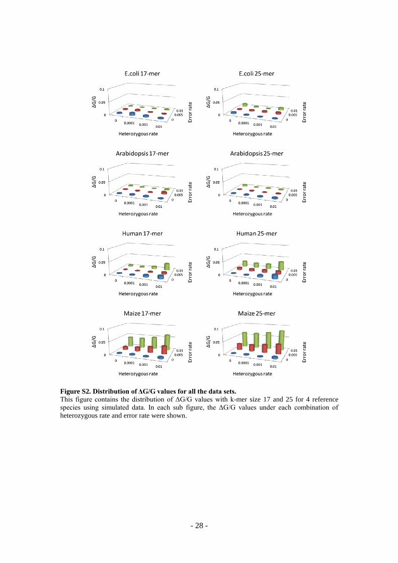
Figure S2. Distribution of ΔG/G values for all the data sets.

This figure contains the distribution of ΔG/G values with k-mer size 17 and 25 for 4 reference

species using simulated data. In each sub figure, the ΔG/G values under each combination of

heterozygous rate and error rate were shown.

- 29 -

Figure S3. Distribution of Δa1/a1 values for all the data sets. This figure contains the distribution of Δa1/a1 values with k-mer size 17 and 25 for 4 reference

species using simulated data. In each figure, the Δa1/a1 values under each combination of

heterozygous rate and error rate are shown.

- 30 -

Figure S4. Distribution of ΔG/G values separated by each affecting factor.

This figure contains the distribution of ΔG/G values from the totally 96 analysis sets separated by

k-mer sizes (a), heterozygous rate (b), error rate (c), and repeat content (d). Note that the X-axis is

in logarithmic scale, whist the Y-axis means accumulated number of data points.

- 31 -

Figure S5. the influence of k-mer size on estimation accuracy.

This figure shows the influence of k-mer size on the accuracy of genome size estimation and ai

estimation. All the estimation accuracy of 17-mer was shown with dash lines, and 25-mer were

shown as full lines. The estimation accuracy from data with sequencing error (f01, 1%) was shown

with triangle and the estimation accuracy from data with heterozygosis (h01, 1%) was shown with

circle. The estimation result from data without sequencing error or heterozygous was shown with

rhombus.

- 32 -

Figure S6. The k-mer species and individuals curves for real data.

This figure contains the k-mer species and individuals curve (K=17) for the 5 species with real

sequencing data. Besides the real curves, the estimated curves by standard model and continuous

model were also shown.

Supplementary tables

Table S1. All the reference ai values calculated from genomic sequences.

Species SnpRate KmerSize a[0.5] a[1] a[1.5] a[2] a[2.5] a[3] a[3.5] a[4] a[4.5] a[5]

Human

0

17 - 0.6762 - 0.1873 - 0.066 - 0.0279 - 0.0138

25 - 0.9674 - 0.0185 - 0.0053 - 0.0025 - 0.0015

0.0001

17 0.0027 0.6734 0.0013 0.186 0.0006 0.0654 0.0004 0.0276 0.0002 0.0136

25 0.0051 0.9623 0.0001 0.0183 0.0001 0.0053 0 0.0025 0 0.0015

0.001 17 0.0258 0.6489 0.0122 0.1756 0.006 0.0604 0.0032 0.0249 0.0019 0.0121

- 33 -

25 0.0942 0.8251 0.0505 0.0147 0.0026 0.0037 0.0012 0.0016 0.0007 0.0009

0.01

17 0.2014 0.4748 0.0776 0.1122 0.0316 0.0349 0.0141 0.0135 0.0071 0.0063

25 0.3646 0.607 0.0071 0.0093 0.0023 0.0024 0.0011 0.001 0.0007 0.0006

Maize

0

17 - 0.7317 - 0.1259 - 0.0446 - 0.0238 - 0.0147

25 - 0.8143 - 0.0883 - 0.0302 - 0.0164 - 0.0101

0.0001

17 0.0047 0.7271 0.0012 0.1247 0.0006 0.044 0.0004 0.0234 0.0003 0.0144

25 0.0069 0.8078 0.001 0.0872 0.0005 0.0297 0.0003 0.0161 0.0002 0.0098

0.001

17 0.0444 0.6889 0.0107 0.1149 0.005 0.0395 0.0031 0.0205 0.0022 0.0123

25 0.0645 0.7537 0.0082 0.0784 0.0039 0.0258 0.0025 0.0136 0.0018 0.0081

0.01

17 0.2975 0.4588 0.052 0.0677 0.0192 0.0219 0.0103 0.0109 0.0064 0.0064

25 0.4064 0.4447 0.0336 0.0399 0.0125 0.0125 0.0067 0.0063 0.0041 0.0037

Arabidopsis

0

17 - 0.9166 - 0.0598 - 0.0114 - 0.0043 - 0.0023

25 - 0.9673 - 0.0216 - 0.0046 - 0.0021 - 0.0012

0.0001

17 0.0033 0.9133 0.0003 0.0594 0.0001 0.0114 0 0.0043 0 0.0023

25 0.005 0.9624 0.0001 0.0215 0 0.0046 0 0.0021 0 0.0012

0.001

17 0.0329 0.8841 0.003 0.0566 0.0008 0.0106 0.0004 0.0039 0.0002 0.0021

25 0.049 0.919 0.0011 0.02 0.0004 0.0042 0.0002 0.0019 0.0001 0.0011

0.01

17 0.2649 0.6575 0.0205 0.0363 0.0043 0.0061 0.0017 0.0021 0.0009 0.001

25 0.3653 0.6085 0.0066 0.0109 0.0017 0.0021 0.0008 0.0009 0.0005 0.0005

Ecoli

0

17 - 0.9906 - 0.005 - 0.0017 - 0.0005 - 0.0004

25 - 0.993 - 0.003 - 0.0015 - 0.0004 - 0.0004

0.0001

17 0.0035 0.9871 0 0.005 0 0.0016 0 0.0005 0 0.0004

25 0.0051 0.9878 0 0.003 0 0.0015 0 0.0004 0 0.0004

0.001

17 0.0333 0.9574 0.0002 0.0048 0.0001 0.0015 0 0.0004 0 0.0004

25 0.0483 0.9448 0.0001 0.0028 0.0001 0.0014 0.0001 0.0003 0 0.0003

0.01

17 0.2717 0.72 0.0014 0.0031 0.0005 0.0009 0.0002 0.0002 0.0001 0.0002

25 0.3638 0.6305 0.001 0.0016 0.0005 0.0007 0.0001 0.0002 0.0002 0.0002

This table contains the reference ai values for each genome with various heterozygous rates. Note

that only the ai (i<=5) values are shown in this Table. Here a[i] is equivalent form with ai, and this

form is also used in the other Tables of this paper.

Table S2. Estimation of heterozygous rate using simulated sequencing data.

Species error k- Het-rate 0 Het-rate 0.01% Het-rate 0.1% Het-rate 1%

- 34 -

rate mer

size a[1/2] estimated het-rate

a[1/2] estimated het-rate

a[1/2] estimated het-rate

a[1/2] estimated het-rate

E.coli_K-

12

0 17 0.20% 0.01% 0.40% 0.01% 3.53% 0.11% 27.26% 0.93%

25 0.15% 0.00% 0.62% 0.01% 5.14% 0.11% 36.49% 0.89%

0.005 17 0.30% 0.01% 0.44% 0.01% 3.82% 0.11% 27.39% 0.93%

25 0.43% 0.01% 0.59% 0.01% 5.44% 0.11% 36.57% 0.90%

0.01 17 0.38% 0.01% 0.55% 0.02% 3.42% 0.10% 27.12% 0.92%

25 0.17% 0.00% 0.77% 0.02% 4.91% 0.10% 36.36% 0.89%

Arabidopsis

0 17 0.14% 0.00% 0.49% 0.01% 3.53% 0.11% 26.62% 0.90%

25 0.13% 0.00% 0.63% 0.01% 5.07% 0.10% 36.48% 0.89%

0.005 17 0.32% 0.01% 0.65% 0.02% 3.62% 0.11% 26.42% 0.90%

25 0.29% 0.01% 0.72% 0.02% 5.04% 0.10% 36.53% 0.89%

0.01 17 3.35% 0.10% 0.84% 0.03% 3.76% 0.11% 26.31% 0.89%

25 4.37% 0.09% 0.97% 0.02% 5.17% 0.11% 36.43% 0.89%

Human

0 17 0.07% 0.00% 0.38% 0.01% 3.18% 0.10% 20.92% 0.69%

25 0.12% 0.00% 0.63% 0.01% 5.60% 0.12% 36.20% 0.88%

0.005 17 0.46% 0.01% 0.71% 0.02% 2.87% 0.09% 20.08% 0.66%

25 0.46% 0.01% 0.91% 0.02% 5.28% 0.11% 36.60% 0.90%

0.01 17 2.98% 0.09% 1.87% 0.06% 3.90% 0.12% 20.19% 0.66%

25 2.32% 0.05% 1.50% 0.03% 5.74% 0.12% 36.33% 0.89%

Maize

0 17 0.08% 0.00% 0.81% 0.02% 4.90% 0.15% 31.30% 1.09%

25 0.08% 0.00% 1.04% 0.02% 6.83% 0.14% 41.71% 1.05%

0.005 17 3.57% 0.11% 3.81% 0.11% 7.51% 0.23% 30.61% 1.06%

25 3.64% 0.07% 4.11% 0.08% 9.60% 0.20% 41.53% 1.05%

0.01 17 6.56% 0.20% 6.88% 0.21% 9.71% 0.30% 30.50% 1.06%

25 6.64% 0.14% 7.12% 0.15% 11.47% 0.24% 41.45% 1.05%

This table contains the estimation of heterozygous rate using simulated sequencing data. Note that

The a[1/2] values were estimated using the heterozygous model, and the estimated heterozygous

rate is calculated using a[1/2] values by formula (11) in the main text.

Table S3. Detailed results of G and a1 estimation with different methods in real data.

Species Error

preproccess

rough estimate standard model continuous model

k-mer num kmer

depth genome size k-mer num

kmer

depth genome size a[1] k-mer num

kmer

depth genome size a[1]

Ant

all 8,957,619,216 26 344,523,816 8,412,768,579 26.99 311,699,465 82.35% 8,424,523,576 28.08 299,968,437 83.32%

corrected 8,420,417,505 27 311,867,315 8,418,025,783 27.77 303,181,843 83.60% 8,418,520,262 27.19 309,661,529 80.58%

filtered 6,176,724,320 18 343,151,351 6,161,110,494 18.93 325,397,589 77.29% 6,163,847,505 19.77 311,771,512 78.40%

E.coli

all 177,595,732 32 5,549,866 170,393,541 32.33 5,270,968 94.96% 170,519,119 32.15 5,304,537 93.95%

corrected 173,615,476 31 5,600,499 173,572,790 31.98 5,428,390 93.86% 173,577,319 33.35 5,204,046 93.59%

filtered 122,818,870 21 5,848,517 122,456,749 21.86 5,601,505 89.38% 122,471,962 22.68 5,400,141 88.93%

Human all 84,840,631,322 28 3,030,022,547 83,726,746,695 28.77 2,909,815,725 66.37% 83,797,402,710 28.08 2,983,982,946 65.12%

- 35 -

corrected 82,507,739,275 28 2,946,704,974 82,498,370,101 28.74 2,870,287,246 66.90% 82,500,224,647 28 2,946,741,792 65.31%

filtered 67,127,996,412 22 3,051,272,564 67,033,584,827 22.97 2,918,462,646 66.00% 67,041,928,286 23.52 2,850,470,598 67.40%

Panda

all 71,779,930,870 28 2,563,568,959 67,652,851,884 28.82 2,347,329,461 72.21% 67,777,715,418 28.28 2,396,293,201 70.63%

corrected 67,461,715,871 28 2,409,346,995 67,357,673,680 28.88 2,332,652,503 72.14% 67,375,272,401 28.42 2,370,340,602 70.35%

filtered 41,137,783,154 16 2,571,111,447 40,800,034,010 16.89 2,415,518,152 71.30% 40,813,266,099 17.54 2,326,443,641 72.16%

Potato

all 22,403,643,321 26 861,678,589 21,143,648,108 26.71 791,473,035 75.61% 21,185,080,846 26.18 809,264,229 73.55%

corrected 21,424,465,114 27 793,498,707 21,405,809,036 27.62 775,067,312 76.05% 21,407,775,752 27.22 786,567,649 73.85%

filtered 14,136,873,771 17 831,580,810 13,994,215,770 16.99 823,523,416 73.65% 14,000,540,319 17.19 814,396,835 74.59%

This table contains the detailed results of G and a1 estimation with different methods in real data.

Note that there are three data types: “all” means all the sequencing data were used to count k-mer

frequency; “corrected” means the data were error corrected before counting k-mer frequency;

“filtered” means all the raw sequencing data were used to count k-mer frequency, but the k-mers

with low quality were filtered. The detailed descriptions for all the estimation methods can be

found in the main text.

Table S4. The kc and ka values for real sequencing data by the continuous model.

Ant E.coli Human Panda Potato

k ak ck ak ck ak ck ak ck ak ck

1 0.00% 0.00 0.00% 0.00 0.00% 0.00 0.00% 0.00 0.00% 0.00

2 0.00% 10.60 0.00% 12.19 0.00% 11.35 0.00% 12.85 0.00% 12.78

3 0.14% 10.78 0.07% 12.21 0.07% 11.39 0.03% 12.90 0.08% 12.94

4 2.79% 11.22 2.59% 12.57 3.37% 11.52 2.24% 13.00 2.13% 13.22

5 5.62% 15.45 8.00% 19.61 4.93% 16.24 5.09% 15.69 5.96% 14.90

6 10.47% 20.31 13.14% 23.78 8.73% 21.29 9.17% 21.97 10.14% 20.36

7 13.88% 23.21 17.65% 28.22 11.40% 24.56 13.49% 24.82 13.92% 23.21

8 15.27% 26.52 19.53% 32.15 12.01% 28.27 14.98% 28.54 15.21% 26.30

9 14.20% 29.76 16.48% 35.24 10.80% 31.59 13.22% 31.53 13.05% 29.21

10 11.39% 32.66 10.50% 38.53 8.62% 34.74 8.51% 34.12 9.21% 31.74

11 7.05% 35.43 5.67% 42.73 5.80% 38.18 5.07% 37.36 5.47% 34.50

12 4.23% 38.45 2.71% 46.35 3.85% 42.12 2.85% 42.32 2.70% 38.47

13 2.46% 42.12 1.15% 49.42 3.04% 46.30 2.38% 47.34 1.89% 43.46

14 1.34% 46.50 0.47% 55.35 2.54% 50.33 2.30% 51.09 1.66% 47.48

15 1.01% 50.95 0.32% 62.96 2.42% 54.04 2.38% 54.28 1.59% 50.60

16 0.89% 54.81 0.25% 65.76 2.29% 57.48 2.37% 57.35 1.58% 53.42

17 0.85% 58.06 0.21% 67.87 2.13% 60.78 2.15% 60.46 1.50% 56.26

18 0.84% 60.95 0.17% 71.02 1.96% 64.09 1.86% 63.67 1.31% 59.23

19 0.79% 63.74 0.14% 76.95 1.68% 67.52 1.45% 67.07 1.11% 62.37

20 0.70% 66.59 0.12% 81.41 1.47% 71.07 1.11% 70.80 0.92% 65.66

21 0.60% 69.63 0.10% 83.70 1.22% 74.75 0.92% 74.95 0.72% 69.14

22 0.47% 72.92 0.08% 86.13 1.03% 78.50 0.77% 79.17 0.61% 72.81

23 0.38% 76.46 0.05% 92.22 0.91% 82.26 0.71% 83.04 0.54% 76.56

24 0.32% 80.23 0.05% 99.46 0.79% 85.97 0.64% 86.47 0.48% 80.17

- 36 -

25 0.27% 84.10 0.04% 101.84 0.73% 89.58 0.58% 89.66 0.46% 83.52

26 0.24% 87.84 0.04% 103.32 0.64% 93.12 0.52% 92.85 0.43% 86.65

27 0.22% 91.29 0.03% 105.35 0.57% 96.63 0.45% 96.24 0.39% 89.69

28 0.21% 94.48 0.02% 112.09 0.52% 100.17 0.39% 99.92 0.36% 92.76

29 0.19% 97.53 0.02% 120.53 0.46% 103.78 0.34% 103.84 0.33% 95.97

30 0.18% 100.60 0.02% 122.71 0.42% 107.42 0.29% 107.78 0.29% 99.39

31 0.16% 103.80 0.02% 123.76 0.38% 111.04 0.27% 111.54 0.26% 102.99

32 0.15% 107.19 0.01% 124.69 0.33% 114.60 0.24% 115.06 0.24% 106.64

33 0.13% 110.74 0.01% 126.26 0.31% 118.15 0.22% 118.45 0.22% 110.17

34 0.12% 114.36 0.01% 136.88 0.27% 121.79 0.20% 121.89 0.21% 113.52

35 0.11% 117.96 0.01% 149.27 0.25% 125.61 0.18% 125.54 0.20% 116.73

36 0.10% 121.53 0.01% 151.18 0.23% 129.58 0.16% 129.49 0.19% 119.95

37 0.10% 125.10 0.01% 152.17 0.21% 133.49 0.15% 133.55 0.18% 123.37

38 0.09% 128.71 0.01% 153.03 0.21% 137.16 0.14% 137.41 0.17% 127.09

39 0.09% 132.38 0.01% 154.14 0.19% 140.57 0.13% 140.94 0.16% 131.07

40 0.09% 136.08 0.01% 156.62 0.18% 143.99 0.12% 144.34 0.16% 135.07

41 0.08% 139.86 0.01% 169.81 0.17% 147.96 0.11% 148.16 0.16% 138.88

42 0.09% 143.92 0.01% 175.48 0.16% 153.47 0.11% 153.39 0.16% 142.64

43 0.09% 148.77 0.01% 176.35 0.17% 160.58 0.11% 160.47 0.16% 147.03

44 0.09% 155.56 0.01% 200.84 0.19% 165.80 0.13% 166.00 0.17% 153.78

45 0.12% 164.11 0.02% 200.84 0.22% 168.92 0.14% 169.25 0.23% 163.43

46 0.17% 171.73 0.03% 200.84 0.16% 178.70 0.11% 177.39 0.33% 170.11

47 0.28% 197.35 0.01% 246.35 0.50% 198.30 0.33% 198.36 0.53% 196.40

48 0.96% 250.58 0.15% 246.35 1.45% 250.07 0.90% 249.91 2.24% 251.20

This file contains the kc and ka values for real sequencing data by the continuous model. Note

that 48 ranks (k) were designed originally to represent i up to 6, with each i has 8 ranks.

Table S5. Comparison of estimation accuracy between GSP and GCE #Species kmer_size error snp gsp_estimate_genome_size gsp_a[1] gce_estimate_genome_size gce_estimate_a[1] gsp_ΔG/G gce_ΔG/G gsp_Δa[1]/a[1] gce_Δa[1]/a[1]

Arabidopsis 17 0.E+00 0.E+00 113993564 0.92 119182048 0.92 4.21% 0.15% 0.70% 0.14%

Arabidopsis 17 5.E-03 0.E+00 114030797 0.37 119227035 0.92 4.17% 0.19% 59.31% 0.14%

Arabidopsis 17 1.E-02 0.E+00 115279632 0.27 119479778 0.90 3.12% 0.41% 70.98% 1.59%

Arabidopsis 25 0.E+00 0.E+00 116529243 0.97 119133663 0.97 2.07% 0.11% 0.18% 0.06%

Arabidopsis 25 5.E-03 0.E+00 116630407 0.33 119112889 0.97 1.99% 0.10% 65.47% 0.05%

Arabidopsis 25 1.E-02 0.E+00 117901514 0.23 119781621 0.95 0.92% 0.66% 76.22% 1.52%

Ecoli 17 0.E+00 0.E+00 4632494 0.99 4654689 0.99 0.15% 0.32% 0.06% 0.07%

Ecoli 17 5.E-03 0.E+00 4677692 0.40 4652932 0.99 0.82% 0.29% 59.42% 0.05%

Ecoli 17 1.E-02 0.E+00 4635012 0.27 4633878 0.99 0.10% 0.12% 72.84% 0.05%

Ecoli 25 0.E+00 0.E+00 4635069 0.99 4667422 0.99 0.10% 0.60% 0.00% 0.07%

Ecoli 25 5.E-03 0.E+00 4634535 0.36 4626684 0.99 0.11% 0.28% 64.25% 0.01%

Ecoli 25 1.E-02 0.E+00 4637042 0.23 4690747 0.99 0.06% 1.10% 76.74% 0.12%

- 37 -

Human 17 0.E+00 0.E+00 1747267956 0.86 2836465136 0.67 38.31% 0.14% 26.59% 0.24%

Human 17 5.E-03 0.E+00 1749246652 0.43 2831972523 0.67 38.24% 0.01% 35.97% 0.21%

Human 17 1.E-02 0.E+00 1762593558 0.35 2848494229 0.67 37.77% 0.57% 48.98% 1.13%

Human 25 0.E+00 0.E+00 2492726920 0.98 2834895501 0.97 11.99% 0.09% 0.89% 0.04%

Human 25 5.E-03 0.E+00 2501613901 0.34 2857474431 0.97 11.68% 0.89% 65.06% 0.11%

Human 25 1.E-02 0.E+00 2516523947 0.23 2896908560 0.96 11.15% 2.28% 76.43% 0.66%

Maize 17 0.E+00 0.E+00 518557098 0.95 2037685440 0.73 74.50% 0.21% 29.15% 0.20%

Maize 17 5.E-03 0.E+00 535682479 0.31 2058430932 0.72 73.66% 1.23% 57.77% 1.52%

Maize 17 1.E-02 0.E+00 571667131 0.22 2116150329 0.71 71.89% 4.07% 70.21% 3.19%

Maize 25 0.E+00 0.E+00 789605809 0.94 2035563354 0.81 61.17% 0.10% 15.56% 0.09%

Maize 25 5.E-03 0.E+00 835513043 0.24 2084690632 0.81 58.91% 2.52% 70.04% 1.05%

Maize 25 1.E-02 0.E+00 871713364 0.16 2161099906 0.80 57.13% 6.28% 80.84% 2.27%

Arabidopsis 17 0.E+00 1.E-04 114223117 0.92 119433737 0.92 4.01% 0.37% 0.70% 0.22%

Arabidopsis 17 5.E-03 1.E-04 114226522 0.37 119141613 0.92 4.01% 0.12% 59.31% 0.25%

Arabidopsis 17 1.E-02 1.E-04 114378568 0.25 119243299 0.92 3.88% 0.21% 72.62% 0.24%

Arabidopsis 25 0.E+00 1.E-04 228266169 0.02 119230332 0.97 91.82% 0.20% 97.83% 0.46%

Arabidopsis 25 5.E-03 1.E-04 116956240 0.33 119109919 0.97 1.72% 0.09% 65.47% 0.46%

Arabidopsis 25 1.E-02 1.E-04 117161156 0.22 119118473 0.97 1.54% 0.10% 77.67% 0.48%

Ecoli 17 0.E+00 1.E-04 4640150 0.99 4682725 0.99 0.01% 0.93% 0.06% 0.27%

Ecoli 17 5.E-03 1.E-04 4641574 0.41 4665487 0.99 0.04% 0.56% 58.81% 0.27%

Ecoli 17 1.E-02 1.E-04 4640646 0.27 4641926 0.99 0.02% 0.05% 72.84% 0.31%

Ecoli 25 0.E+00 1.E-04 4646552 0.99 4648897 0.99 0.15% 0.20% 0.00% 0.50%

Ecoli 25 5.E-03 1.E-04 4647218 0.36 4659834 0.99 0.16% 0.43% 64.05% 0.47%

Ecoli 25 1.E-02 1.E-04 4645871 0.23 4620763 0.99 0.13% 0.41% 76.74% 0.50%

Human 17 0.E+00 1.E-04 1750534529 0.86 2838372887 0.67 38.20% 0.21% 26.59% 0.22%

Human 17 5.E-03 1.E-04 1751831553 0.43 2830714668 0.68 38.15% 0.06% 35.97% 0.24%

Human 17 1.E-02 1.E-04 1760548923 0.34 2841008485 0.67 37.84% 0.31% 50.01% 0.07%

Human 25 0.E+00 1.E-04 2499463943 0.98 2835970370 0.97 11.75% 0.13% 0.89% 0.50%

Human 25 5.E-03 1.E-04 2507460686 0.34 2856020286 0.97 11.47% 0.84% 65.06% 0.43%

Human 25 1.E-02 1.E-04 2520527244 0.22 2885870063 0.97 11.01% 1.89% 77.36% 0.32%

Maize 17 0.E+00 1.E-04 520388042 0.95 2041728303 0.73 74.41% 0.41% 29.15% 0.33%

Maize 17 5.E-03 1.E-04 536702116 0.31 2065464402 0.72 73.61% 1.57% 57.77% 1.02%

Maize 17 1.E-02 1.E-04 572587757 0.22 2116256118 0.71 71.84% 4.07% 70.21% 2.57%

Maize 25 0.E+00 1.E-04 793501673 0.94 2040454389 0.81 60.98% 0.34% 15.56% 0.62%

Maize 25 5.E-03 1.E-04 838042754 0.24 2086280421 0.81 58.79% 2.60% 70.04% 0.25%

Maize 25 1.E-02 1.E-04 873744098 0.16 2161275222 0.80 57.03% 6.28% 80.72% 1.48%

Arabidopsis 17 0.E+00 1.E-03 116178157 0.92 119469709 0.87 2.37% 0.40% 0.70% 1.70%

Arabidopsis 17 5.E-03 1.E-03 116126936 0.38 119205642 0.87 2.41% 0.17% 58.98% 1.55%

Arabidopsis 17 1.E-02 1.E-03 116483834 0.25 119655679 0.87 2.11% 0.55% 72.29% 1.92%

Arabidopsis 25 0.E+00 1.E-03 119778936 0.97 119284430 0.91 0.66% 0.24% 0.07% 1.34%

Arabidopsis 25 5.E-03 1.E-03 119694666 0.34 118930497 0.91 0.59% 0.06% 65.06% 0.90%

Arabidopsis 25 1.E-02 1.E-03 119868482 0.22 119258955 0.91 0.73% 0.22% 77.36% 1.37%

Ecoli 17 0.E+00 1.E-03 4714392 0.99 4664276 0.95 1.61% 0.53% 0.06% 1.28%

Ecoli 17 5.E-03 1.E-03 4712400 0.41 4631437 0.94 1.57% 0.18% 58.61% 1.30%

Ecoli 17 1.E-02 1.E-03 4711747 0.27 4644340 0.95 1.55% 0.10% 72.54% 0.95%

Ecoli 25 0.E+00 1.E-03 4754346 0.99 4637500 0.93 2.47% 0.05% 0.10% 1.08%

Ecoli 25 5.E-03 1.E-03 4755820 0.36 4612603 0.93 2.50% 0.58% 63.65% 1.18%

Ecoli 25 1.E-02 1.E-03 4743675 0.24 4642938 0.94 2.24% 0.07% 76.33% 0.93%

Human 17 0.E+00 1.E-03 1781877085 0.85 2852338189 0.62 37.09% 0.71% 26.00% 3.96%

- 38 -

Human 17 5.E-03 1.E-03 1775011701 0.44 2840889922 0.63 37.33% 0.30% 35.67% 2.33%

Human 17 1.E-02 1.E-03 1779351166 0.34 2859731024 0.62 37.18% 0.97% 49.87% 5.18%

Human 25 0.E+00 1.E-03 2560242878 0.98 2850753099 0.89 9.61% 0.65% 0.79% 7.83%

Human 25 5.E-03 1.E-03 2568748123 0.34 2862009236 0.91 9.31% 1.05% 64.54% 9.84%

Human 25 1.E-02 1.E-03 2586399277 0.22 2888544012 0.90 8.68% 1.98% 76.95% 9.15%

Maize 17 0.E+00 1.E-03 536585544 0.95 2039037547 0.68 73.61% 0.27% 29.15% 1.54%

Maize 17 5.E-03 1.E-03 551339418 0.32 2079155376 0.63 72.89% 2.25% 56.68% 8.13%

Maize 17 1.E-02 1.E-03 580792069 0.22 2132256530 0.60 71.44% 4.86% 70.07% 12.60%

Maize 25 0.E+00 1.E-03 827749160 0.94 2037667192 0.74 59.29% 0.21% 15.56% 1.29%

Maize 25 5.E-03 1.E-03 860151082 0.25 2098695048 0.70 57.70% 3.21% 69.42% 6.99%

Maize 25 1.E-02 1.E-03 904636916 0.16 2174457885 0.68 55.51% 6.93% 80.60% 10.37%

Arabidopsis 17 0.E+00 1.E-02 137172546 0.90 119502846 0.65 15.27% 0.42% 2.25% 1.09%

Arabidopsis 17 5.E-03 1.E-02 137057183 0.40 119438723 0.65 15.18% 0.37% 56.91% 0.83%

Arabidopsis 17 1.E-02 1.E-02 138144123 0.27 120170377 0.65 16.09% 0.99% 70.43% 0.76%

Arabidopsis 25 0.E+00 1.E-02 218874698 0.45 119464058 0.60 83.93% 0.39% 53.69% 0.81%

Arabidopsis 25 5.E-03 1.E-02 217156887 0.18 118803053 0.60 82.49% 0.16% 81.29% 0.77%

Arabidopsis 25 1.E-02 1.E-02 216070832 0.12 119285241 0.60 81.58% 0.24% 87.28% 0.81%

Ecoli 17 0.E+00 1.E-02 5615290 0.94 4653027 0.71 21.03% 0.29% 4.81% 1.07%

Ecoli 17 5.E-03 1.E-02 5603955 0.42 4636462 0.71 20.78% 0.07% 57.40% 1.11%

Ecoli 17 1.E-02 1.E-02 5699551 0.28 4650758 0.72 22.84% 0.24% 71.63% 0.67%

Ecoli 25 0.E+00 1.E-02 9133062 0.38 4643339 0.63 96.85% 0.08% 61.73% 0.84%

Ecoli 25 5.E-03 1.E-02 9114588 0.16 4609669 0.63 96.45% 0.65% 84.39% 0.62%

Ecoli 25 1.E-02 1.E-02 9128281 0.10 4597866 0.63 96.74% 0.90% 89.53% 0.26%

Human 17 0.E+00 1.E-02 2054684008 0.83 2865254085 0.45 27.46% 1.16% 22.89% 4.23%

Human 17 5.E-03 1.E-02 2047915840 0.46 2852169971 0.47 27.70% 0.70% 32.42% 0.04%

Human 17 1.E-02 1.E-02 2061230383 0.37 2908235720 0.46 27.23% 2.68% 45.58% 3.38%

Human 25 0.E+00 1.E-02 3129041400 0.96 2874261953 0.59 10.47% 1.48% 0.56% 2.51%

Human 25 5.E-03 1.E-02 3123422298 0.38 2864463640 0.60 10.28% 1.13% 60.51% 0.78%

Human 25 1.E-02 1.E-02 3183400262 0.26 2930637221 0.59 12.39% 3.47% 72.71% 3.22%

Maize 17 0.E+00 1.E-02 695819120 0.94 2046699465 0.45 65.78% 0.65% 28.60% 1.83%

Maize 17 5.E-03 1.E-02 719596150 0.37 2096864740 0.45 64.61% 3.12% 49.98% 1.72%

Maize 17 1.E-02 1.E-02 752269146 0.26 2162585546 0.44 63.01% 6.35% 64.47% 3.69%

Maize 25 0.E+00 1.E-02 1160175379 0.94 2047298540 0.44 42.95% 0.68% 15.19% 1.30%

Maize 25 5.E-03 1.E-02 1202324526 0.30 2111723426 0.44 40.87% 3.85% 62.67% 1.45%

Maize 25 1.E-02 1.E-02 1202098973 0.19 2198481293 0.43 40.88% 8.11% 76.42% 3.79%

This table contains the detailed results for GSP and GCE estimation results, including the genome

size, a1 values, and all the middle results.

Supplementary methods

1 k-mer frequency counting

Counting k-mer frequency from either the reference genome sequence or sequenced reads

data is one of the most fundamental analyses in bioinformatics. To estimate genomic characters,

the k-mer size (K) should be determined under the logic that the space of k-mers (4K) should be

- 39 -

several times larger than the genome size (G), so that few k-mers derived from different genomic

positions will merge together by chance, i.e. most k-mers in the genome will appear uniquely. In

practice, we often require the k-mer space to be at least 5 times larger than the genome size

(4K

>5*G), and the larger the better. When the k-mer size for a special application is determined,

the next question is to find an appropriate tool to count k-mer frequency. From our experience, the

recently published jellyfish algorithm [1] performs better than the others, which has relatively

faster running speed and smaller memory requirement, as well as broader accessible range of k-

mer size (up to 31 bp). Note that the computer memory consumption for k-mer frequency counting

is often very large, especially for data from large genome and which has many sequencing errors,

so you’d better pre-estimate the memory usage and find a computer with enough memory to run

the task. When the estimated memory usage exceeds that of the largest-memory computer you can

access, then the only way is to choose or design some memory saving algorithms such as bloom

filter [2]. We do not discuss more details on k-mer counting algorithms here, because it is not the

focus of this paper.

We also developed a counting k-mer program named as kmerfreq, which contains two

methods: “kmer_freq_array” uses the array index to represent k-mers, and requires 4K computer

memory for any data; “kmer_freq_hash” uses hash key to store k-mers, although it requires much

more memory to store one k-mer, however the memory requirement is in line with the number of

k-mer species in the given data. For smaller k-mer size (K<=17), it is better to use

“kmer_freq_array”, while for larger k-mer size (K<=27), “kmer_freq_hash” will be the preferred.

2 Estimation of the expected coverage depth of k-mer (c)

2.1 Estimating c based on definition

For genomes without repeat, it is defined as that:

( ) Kindividuals Kindividuals

Kspecies

n nc xp x

n G , Kspeciesn G

For genomes with repeat, it can be calculated by:

/( )

* /

Kindividuals Kspecies Kindividuals

i Kspecies

n nxp x nc

i a G n G

2.2 Estimating c from Poisson distribution

For genomes without repeat, ( )KspeciesP x follows the Poisson distribution. Then:

( )!

xc

Kspecies

cP x e

x

- 40 -

( 1)

( ) ( ) /! 1 !

x xc c

Kindividuals Kspecies

xc cP x xP x c e e

x c x

By deduction, we can get:

1

( ) 1!

( 1)

( 1)!

xc

Kspecies

xcKspecies

ceP x xx

cP x ce

x

1

( ) ( 1)!

( 1)

!

xc

Kindividuals

xcKindividuals

ce

P x xx

cP x ce

x

Thus, we can estimate c based on the following formula:

( 1)( 1)

( )

Kspecies

Kspecies

P xc x

P x

( 1)

( )

Kindividuals

Kindividuals

P xc x

P x

3 Exploring the repetitive genomes

The real genomes often contain huge amount of repeat sequences, including transposable elements

[3], tandem repeats [4], and segmental duplications [5], which bring great challenge in the

assembly processes [6]. The ai and bi values calculated by genomic k-mer frequency and the k-mer

species and individuals curves plotted by coverage depth, are closely related with repeats in the

genome. We can make a rough inference that the genome contains repeats if we see multiple peaks

on the k-mer species and individuals curves. To be more quantitative and intuitionistic to reflect

genomic repeat character, it is better to use the ai and bi values at the same time.

Calculating genome size for repetitive genomes based on the compound Poisson model:

,

, , ,

1 1 1

1m m mi Kindividuals Kindividuals kmer

i genomic Kspecies i Kindividuals

i i ii

n n nG i n i n

c c c c

Note: For the number of k-mer species and individuals, if not specified as “genomic”, it

means in the sequencing data.

4 The standard model

For genome with various copies of repeat families, we can divide the genome sequence into

- 41 -

m repeat families, and let i∈[1,m] be the copy number of the ith repeat families (also the genomic

frequency of contained k-mers). We define ai as the ratio (probability) of k-mer species with

genomic frequency i divided by total k-mer species and bi as the ratio (probability) of k-mer

individuals with genomic frequency i divided by total k-mer individuals. Then the whole genome

will be sequenced randomly, and the k-mer frequency will be counted from the sequenced reads.

There is a coverage depth character for each sequenced k-mer,which is ranging from 1 to w. For

each coverage depth, we define vj as the ratio of jth depth k-mer species divided by total k-mer

species and uj as the ratio of jth depth k-mer individuals divided by total k-mer individuals. It is

supposed that the sequencing on each repeat part is independent, so for the k-mers with same

genomic frequency i, the depth distribution is also following a Poisson distribution. Then we can

use the following compound model to describe the total k-mer depth distribution:

,

1

( ) ( )m

Kspecies i Kspecies i

i

P x a P x

,

1

( ) ( )m

Kindividuals i Kindividuals i

i

P x b P x

Because i is integer and stands for the copy number of the k-mer in the genome, we can get

the following formula:

ic i c , c is the k-mer depth of the unique region.

, ,

,

1 1 1

1m m mi Kindividuals i Kindividuals Kindividuals

i Kindividuals

i i ii

n n nG i i n

c i c c c

The relation between ia and ib is:

Kspecies i i

i

k mer

n a cb

n

Because there is relation between ai and bi, we just estimate ai in the bellow.

To estimate ai, we have the prior probabilities:

( ) iP i a , ( )

( | )!

j icic eP j i

j

1 1

( | )( ) ( | )( | )

( ) ( | ) ( | )

i

m m

i

i i

a P j iP i P j iP i j

P i P j i a P j i

The posterior probabilities can be calculated by:

0

( | )w

i j

j

a P i j v

Then we get the iteration formula:

- 42 -

,

, 1

0,

1

( | )

( | )

wi t

i t jmj

i t

i

a P j ia v

a P j i

,1, 1

1

,1, 1

( 1)( 1)

( )

Kspecies t

t

Kspecies t

P xc x

P x

, 1 1i t tc i c

In each iteration cycle, we update ia and remove the repeat parts from the raw depth

distribution curve, then only the unique curve is left and used to estimate the unique depth c and

update ic .

When j=0, the 0v can not be counted directly from reads, which stands for the uncovered

region in the genome. Although the sequencing depth is quite high for short read sequencing, there

are still some regions not covered by reads. Here we still use the Lander-Waterman model in 1988

to estimate the uncovered gap region. For each ith repeat region, the expected k-mer depth is ci,

then the gap probability is ice

, so we can estimate the 0v by:

0

1

mic

i

i

v a e

5 Exploring the heterozygous genomes

For heterozygous genomes, the heterozygous sites may cause a new set of peaks on the k-mer

coverage depth distribution curves with the peak position at i*c/2 named as hybrid peaks. For non-

repetitive genome, when the heterozygous rate gets higher, another peak rises at the c/2 position.

Moreover, when the heterozygous rate passes a threshold, the c/2 peak will become the major peak

replacing that at depth c. It also shows that the two curves have different advantage for different

purposes. It is easier to find out the homozygous peak (c) in the k-mer individual curve when the

heterozygous rate is relatively high, while it is easier to find out the heterozygous peak (c/2) in k-

mer species curve when the heterozygous rate is relatively low.

We developed the heterozygous discrete model for heterozygous genome, in which i is integer

times of 1/2. In practice, the height of hybrid peaks may increase as the heterozygous rate gets

higher and it might be difficult to distinguish the repeat peaks and the hybrid peaks. Then we need

additional biological background of the sequencing sample to make a correct determination.

Heterozygous rate is a quite important character for genome sequencing projects. For non-

repetitive genome, when the 4K is much larger than the genome size, one heterozygous site will

cause K new k-mers and 2*K k-mers with coverage depth c/2, then we can get the formula (11) to

roughly estimate the heterozygous rate for diploid genome. For repetitive genome, there is no

- 43 -

clear relationship between the ai and heterozygous rate, so it is difficult to make a formula.

However, in practice, we can still use formula (11) to roughly estimate the heterozygous rate for

diploid genome with repeats, although it is not as accurate as that of non-repetitive genome.

6 Sequencing error model

For reads data with sequencing error, we can divide the erroneous k-mer into two kinds. The

first kind of erroneous k-mer has low depth and do not exist in the genome. They have the

expected depth,error outc . The other kind erroneous k-mers exist in the genome and merge with the

correct k-mers increasing their expected depth. Let ,error inc be the increment, then we can get the

compound model:

, ,

1

, ,

, ,

4( ) ( ) ( )

4

4

( ) Poisson( )

( ) Poisson( )

kmKspecies

Kspecies i Kspecies i Kspecies errorki

Kspecies

i ik

Kspecies i error in

Kspecies error error out

nP x A P x P x

nA a

P x c c

P x c

The ,error outc and ,error inc are related to the sequencing error rate, the k-mer size and the

genome size， and they are quite difficult to be estimated in practice, so this sequencing error

model was not used later.

To reduce the influence of erroneous k-mers, we suggest filtering k-mers by sequencing

quality when counting the k-mer frequency. Here we calculate the probability that a k-mer is

correct with the following formula:

10( , ) 10S

iP base error e

1

( , ) (1 )K

i

i

P Kmer correct e

Note: S refer to the Phred scale score, which can be generated by most sequencing platforms.

To filter most of the erroneous k-mers, we require all the k-mers being counted to have P(Kmer,

correct) larger than a threshold, for example, 0.95.

7 Continuous compound model

Previous studies have shown that several factors may cause coverage bias, including uneven

- 44 -

GC content and specific sequence structure [7-9]. Then for real sequencing data, the coverage

depth of sequenced k-mer is not only dependent on its genomic frequency, but also dependent on

the sequencing bias characters, so we define the observed genomic frequency i when sequencing

coverage bias exists. The value of i will be continuous. It is supposed that the sequencing on each

group with same observed genomic frequency i is independent, so for the k-mers from the same

ith group, the depth distribution is also following a Poisson distribution. Referring to the discrete

compound model, we can get the continuous compound model to describe the total k-mer

coverage depth distribution for real sequencing data:

,( ) ( )Kspecies i Kspecies i

P x a P x di

,( ) ( )Kindividuals i Kindividuals i

P x b P x di

Note: i

a and i

b are the observed value for each continuous i , which are different to the

genomic ia and ib . To make it easy, we used the following dense discrete model in practice:

,

1

( ) ( )m

Kspecies k Kspecies k

k

P x a P x

,

1

( ) ( )m

Kindividuals k Kindividuals k

k

P x b P x

Note: m is the total Poisson distribution number or peak number we considered. The

symbol k here just stands for the peak order, and there is no relation between k and kc . Then we

estimate the kc and ka with the following iteration formulas:

( | )!

kcj

kc eP j k

j

,

, 1

0 ,

( | )

( | )

j wk t

k t j

j k t

k

a P j ka v

a P j k

, 1

0 , 10

, 1

, 1 , 1

( | )

( | ) ( | )

wk tw

jj j k t

j kk t

k t k t

a P j kj v

j P k j v a P j k

ca a

After we have estimated ka and kc , we need to determine the coverage depth c and genomic

ai. Supposing that most of the genomic unique k-mers are not affected by coverage bias, so in

practice, we can either use the kc with the highest ka in the unique peak region as the coverage

depth c, or use the average kc around the highest ka to stand for the genomic coverage depth c.

However, it is quite difficult to estimate the relationship between ka and ia , because we can not

- 45 -

model the sequencing coverage bias right now. Then in practice, we just calculate genomic 1a by

summarizing the ka values around the unique peak.

8 Dealing with sequencing error and coverage bias

To estimate the genome size by formula (2), we need to make clear the distribution of erroneous k-

mers and estimate the parameters n and c for correct k-mers from the mixture k-mer coverage

depth distribution. We have designed a united model to represent erroneous and correct k-mers

together in this paper, however, the model is affected by many genomic and sequencing characters

and thus quite difficult to resolve. Instead, we turned to use a simple experience based method to

exclude the erroneous k-mers caused by sequencing errors. During each cycle of the Bayes

iteration, the missing ratio values of k-mer species with depths lower than the threshold should

also be re-calculated by the compound Poisson model with the input c and ai values like

calculating v0 in standard model.

Previous studies have shown that several factors may cause coverage bias, including uneven GC

content and specific sequence structure [7-9]. In theory, although there may be some types of

coverage bias that change the position of the major peak depth as well as the shape of the

distribution curve, from our experience, the major peak depth from distribution curves with

coverage bias still roughly reflects the expected coverage depth for the unique k-mer class (c)

within most real sequencing data.

Supplementary results

1 Estimating with various types of simulated data

We used ΔG/G to evaluate the accuracy of genome size estimation. Among the 96 analysis results,

the largest ΔG/G value is 8.11%, which belongs to maize species with 1% heterozygous rate and

1% error rate and 25 k-mer size. We found that sequencing error is the most difficult factor to deal,

because when the reads data has higher rate of sequencing error, it is more difficult to exclude the

erroneous k-mers from the mixture distribution by the experience-based method. We also found

the k-mer size influence the estimation accuracy. When there is sequencing error or heterozygosity,

ΔG/G of 25-mer are relatively higher than that of 17-mer, which can be explained by that larger k-

mer size will enhance the effect of heterozygosity and sequencing error, moreover, larger k-mer

size also results in lower ck-mer, which tends to decrease the estimation accuracy. Then at cases

with no sequencing error or heterozygosity problems, larger k-mer size will generate more

- 46 -

accurate estimation result by having more advantage to deal with repeat.

The evaluation of ai estimation and the analysis of influencing factors are much more complex

than that of genome size. It is not only caused by the mixture effect of repeat and heterozygosity,

but also related with the applied models (standard or heterozygous model). For simple, we used

Δa1/a1 to evaluate the accuracy of ai estimation. Among the 96 analysis results, the largest Δa1/a1

value is 12.6%, which belongs to Maize species with 0.1% heterozygous rate and 1% error rate

and 17 k-mer size.

2 Analyzing real sequencing data from de novo genome projects

By filtering the low-quality k-mers, there will be much less erroneous k-mers in the result, which

not only makes it easier to estimate the total number of correct k-mer individuals but also

significantly decrease the consumption of computer memory.

Taking the reported genome sizes in the published papers as reference, we calculated the ΔG/G

values for the estimated genome sizes from various methods. About 22% and 80% of the ΔG/G

values are smaller than 1% and 5% respectively, with one largest ΔG/G value of 10% for ant with

all raw k-mers by rough estimation. Then we calculated the reference a1 values from the

assembled genome sequence and used it as a reference to calculate the Δa1/a1 values, among

which 17% and 80% of the Δa1/a1 values are smaller than 1% and 5% respectively, with the

largest Δa1/a1 value of 11% for ant low-quality filtered data with standard model.

There is observed difference between the estimated and reference a1 (b1) values. Besides the

reasons described in the main text, the sequencing coverage bias and the uncertainty relationship

between estimated ka values and genomic ai values should be the most influencing factor that

caused this difference. Although the estimation accuracy is not as high as that of simulated data,

the trends is still correct, and we can roughly infer that 15-mer is enough large to assemble Ecoli

genome, whist larger than 25-mer is proper for assembling the human genome.

For real sequencing data with coverage bias, only when there is observable c/2 peak caused by

heterozygosity, the heterozygous rate can be detected and roughly inferred. It is necessary to

mention that the models in this paper are based on some special hypotheses, so for real sequencing

data, when there is no clear peak which may be caused by low sequencing depth or high

sequencing bias, the data is not qualified for genomic character estimation.

- 47 -

References

1. Marcais G, Kingsford C: A fast, lock-free approach for efficient parallel counting of

occurrences of k-mers. Bioinformatics (Oxford, England) 2011, 27(6):764-770.

2. Melsted P, Pritchard JK: Efficient counting of k-mers in DNA sequences using a bloom

filter. BMC bioinformatics 2011, 12:333.

3. Wicker T, Sabot F, Hua-Van A, Bennetzen JL, Capy P, Chalhoub B, Flavell A, Leroy P,

Morgante M, Panaud O et al: A unified classification system for eukaryotic transposable

elements. Nature reviews 2007, 8(12):973-982.

4. Benson G: Tandem repeats finder: a program to analyze DNA sequences. Nucleic acids

research 1999, 27(2):573-580.

5. She X, Cheng Z, Zollner S, Church DM, Eichler EE: Mouse segmental duplication and copy

number variation. Nature genetics 2008, 40(7):909-914.

6. Miller JR, Koren S, Sutton G: Assembly algorithms for next-generation sequencing data.

Genomics, 95(6):315-327.

7. Bentley DR, Balasubramanian S, Swerdlow HP, Smith GP, Milton J, Brown CG, Hall KP,

Evers DJ, Barnes CL, Bignell HR et al: Accurate whole human genome sequencing using

reversible terminator chemistry. Nature 2008, 456(7218):53-59.

8. Nakamura K, Oshima T, Morimoto T, Ikeda S, Yoshikawa H, Shiwa Y, Ishikawa S, Linak

MC, Hirai A, Takahashi H et al: Sequence-specific error profile of Illumina sequencers.

Nucleic acids research.

9. Dohm JC, Lottaz C, Borodina T, Himmelbauer H: Substantial biases in ultra-short read

data sets from high-throughput DNA sequencing. Nucleic acids research 2008,

36(16):e105.