NBER WORKING PAPER SERIES

ESTIMATING TRADE ELASTICITIES:DEMAND COMPOSITION AND THE TRADE COLLAPSE OF 2008-09

Matthieu BussièreGiovanni Callegari

Fabio GhironiGiulia Sestieri

Norihiko Yamano

Working Paper 17712http://www.nber.org/papers/w17712

NATIONAL BUREAU OF ECONOMIC RESEARCH1050 Massachusetts Avenue

Cambridge, MA 02138December 2011

For helpful comments and discussions at various stages of this project, we thank James Anderson,Philippe Bacchetta, Andrew Bernard, Michele Cavallo, Steven Davis, Robert Feenstra, Joseph Gruber,Luca Guerrieri, Elhanan Helpman, Leonardo Iacovone, Jean Imbs, Olivier Jeanne, Robert Kollmann,John Leahy, Benjamin Mandel, Andrew Rose, Katheryn Russ, Linda Tesar, Shang-Jin Wei, and seminarand conference participants at ASSA 2011, the Banque de France, the Board of Governors of the FederalReserve System, Brandeis University, BRUEGEL, the ECB, the Federal Reserve Bank of Boston,the NBER ITI Spring 2011 meeting, the workshop on "Challenges in Open Economy Macroeconomicsafter the Financial Crisis" at the Federal Reserve Bank of St. Louis, and the BdF/PSE Conference on"The Financial Crisis: Lessons for International Macroeconomics." We are grateful to Jonathan Hoddenbaghfor carefully reviewing our theoretical work. Remaining errors are our responsibility. Work on thispaper was done while Callegari was an Economist at the International Monetary Fund, and Ghironiwas a Visiting Scholar at the Federal Reserve Bank of Boston. The support of these institutions isacknowledged with gratitude. The views expressed in this paper are those of the authors and do notnecessarily reflect official views or policies of the Banque de France, the European Central Bank,the Federal Reserve Bank of Boston, the International Monetary Fund, the National Bureau of EconomicResearch, or the Organisation for Economic Co-operation and Development.

NBER working papers are circulated for discussion and comment purposes. They have not been peer-reviewed or been subject to the review by the NBER Board of Directors that accompanies officialNBER publications.

© 2011 by Matthieu Bussière, Giovanni Callegari, Fabio Ghironi, Giulia Sestieri, and Norihiko Yamano.All rights reserved. Short sections of text, not to exceed two paragraphs, may be quoted without explicitpermission provided that full credit, including © notice, is given to the source.

Estimating Trade Elasticities: Demand Composition and the Trade Collapse of 2008-09Matthieu Bussière, Giovanni Callegari, Fabio Ghironi, Giulia Sestieri, and Norihiko YamanoNBER Working Paper No. 17712December 2011JEL No. F10,F15,F17,F4

ABSTRACT

This paper introduces a new methodology for the estimation of demand trade elasticities based onan import intensity-adjusted measure of aggregate demand, with the foundation of a stylized theoreticalmodel. We compute the import intensity of demand components by using the OECD Input-Outputtables. We argue that the composition of demand plays a key role in trade dynamics because of thelarge movements in the most import-intensive categories of expenditure (especially investment, butalso exports). We provide evidence in favor of these mechanisms for a panel of 18 OECD countries,paying particular attention to the 2008-09 Great Trade Collapse.

Matthieu BussièreBanque de France31 rue Croix des Petits Champs75001 ParisFrancematthieu.bussiere@banque-france.fr

Giovanni CallegariEuropean Central BankKaiserstrasse 2960311 Frankfurt am MainGermanygiovanni.callegari@ecb.int

Fabio GhironiBoston CollegeDepartment of Economics140 Commonwealth AvenueChestnut Hill, MA 02467-3859and NBERfabio.ghironi@bc.edu

Giulia SestieriBanque de France31 rue Croix des Petits Champs75001 ParisFrancegiulia.sestieri@banque-france.fr

Norihiko YamanoOECD2 rue Andre Pascal75775 Paris Cedex 16, ParisFrancenorihiko.yamano@oecd.org

1 Introduction

The relation between trade flows and aggregate macroeconomic dynamics is a central question in

international economics at least since Houthakker and Magee’s (1969) seminal work on the estimation

of income and price elasticities of trade. The issue has received renewed attention, and the debate on

the determinants of trade flows has re-heated, as scholars debated the adjustment of the global trade

imbalances that emerged in the 2000s and struggled to understand the dynamics of world trade in

the aftermath of the global financial crisis of 2008-09. One of the key features of the global recession

triggered by this crisis was a sharp contraction in world trade that reached its peak between the end

of 2008 and the beginning of 2009. In 2009, global trade fell by 11% in real terms on a year-on-year

basis—an unprecedented development since 1945. A distinct feature of this Great Trade Collapse

(GTC; Baldwin, 2009) is that the fall in world trade has been much more pronounced than the fall

in world output (real world GDP dropped by 0.7% in 2009). The change in global trade was higher

than that of global output by a factor of 16 in 2009, against an average of 1.9 in the 1990-2008 period

(Figure 1). The fall in international trade affected a large number of countries in all main economic

regions, albeit to a different extent (Figure 2).

In this paper we re-examine the relation between trade flows and macroeconomic dynamics by

developing a new methodology for the estimation of trade elasticities—specifically, the elasticity

of import demand to aggregate demand—that takes into account the different import content and

cyclical behavior of the different components of aggregate demand. We use the OECD Input-Output

tables to show that the most procyclical components of demand (investment and exports) have a

particularly rich import content, whereas the other components (private consumption and, especially,

government spending) have lower import content. As a result, the fall in imports during recessions

typically exceeds that of GDP by a considerable magnitude, due to the sharp reduction in the

components of GDP that have the highest import content. The fall in investment is often larger

than that of GDP, which triggers a sharp contraction in imports (investment being a particularly

import-intensive category of expenditure). By contrast, government spending and, to a lesser extent,

private consumption are not affected as much, but this does not dampen the fall in imports due to the

relatively lower import content of these categories of expenditure.1 This mechanism was especially

strong during the 2008-09 GTC, during which the fall in imports was ten times larger than the fall

in GDP.2

Armed with these observations and intuition, we construct a new measure of aggregate demand,

which we call IAD (for Import-intensity-Adjusted Demand) as a weighted average of traditional

1Note that, even if investment and exports are unconditionally more volatile than GDP, and consumption issmoother, a closer look at the data shows that the most procyclical components of aggregate demand fall more sharplyduring recessions than they rise in expansions as we review in our empirical work.

2In the United States, for instance, the annualized fall in total investment in the last quarter of 2008 and in thefirst quarter of 2009 was about 24% and 31%, respectively, whereas GDP—partly supported by government spending—contracted by “only” 9.2% and 6.8%.

1

aggregate demand components (investment, private consumption, government spending, and exports)

using as weights the import contents of demand computed from the OECD Input-Output tables. We

show that IAD is highly correlated with GDP, but more volatile on average (especially during

recessions). We provide a theoretical foundation for IAD as the appropriate measure of aggregate

demand in empirical trade equations by relying on a translog GDP function, following Feenstra

(2003a, Chapter 3), Kee, Nicita, and Olarreaga (2008), and a series of articles by Kohli (1978; 1990a,b;

1993). We show that this approach yields a parsimonious, estimable import demand equation in

which imports depend on aggregate demand and relative import prices in the same fashion as implied

by the traditional C.E.S. demand system, but for two important differences: First, IAD replaces the

C.E.S. aggregate demand co mposite as the appropriate measure of aggregate demand. Second, the

elasticity of import demand to (the correct measure of) aggregate demand is no longer restricted to

one.

We take this new empirical model to the data using a panel of 18 OECD countries over the

period 1985Q1-2010Q2 (the choice of countries reflects data availability: The empirical exercise

requires sufficiently long time series to be able to capture a sufficient number of business cycles). We

find that IAD is superior to the standard, alternative measures of aggregate demand used in the

literature in terms of both goodness of fit and, importantly, stability of parameter estimates. The

IAD-based model performs remarkably well in explaining the GTC compared to the alternatives:

Our basic specification explains 85% of the average fall in imports in the G7 countries in 2009Q1

against 51% when using GDP as explanatory variable. The regression using IAD explains 93% of

the fall in imports when the additional demand component “change in inventories” is added to the

regression. Most importantly, the empirical model outperforms the alternatives over the entire sample

period, not just during the recent crisis, yielding estimated elasticities of imports to (the appropriate

measure of) aggregate demand that are significantly less volatile across the different phases of the

cycle.

According to the model, there is no major “puzzle” in the magnitude of the fall in world trade

observed during the recent financial crisis: Trade fell mostly because demand crashed globally and

did so particularly in its most import-intensive component—investment. Moreover, the strong re-

lationship between exports and imports in each country (in 2005, the average import content of

exports was 28% for the sample of countries, and 23% for the G7), linked to the increased interna-

tionalization of production and the strong dependence of the tradable sector on imported inputs,

contributed to the simultaneity and unprecedented severity of the trade collapse. Our approach and

results confirm Marquez’s (1999) argument that using standard measures of aggregate demand, such

as GDP or domestic demand, in trade equations may be misleading, and more so in periods in which

the more import-intensive components of aggregate demand (i.e., investment and exports) fluctuate

2

much more than the others, such as the 2008-09 crisis.3

Finally, the theoretical and empirical implications of the model go some way toward explaining

the so-called Houthakker-Magee puzzle. This puzzle arises when regressing real imports on measures

of aggregate demand and relative import prices yields a coefficient for the demand variable that is

significantly larger than one (a result first found by Houthakker and Magee, 1969, and subsequently

confirmed in a large number of studies). This result is traditionally viewed as a puzzle because a

coefficient above one implies that the ratio of imports to GDP should be above 100% in the long

run. While this may be realistic for small open economies, it is clearly at odds with stylized facts

for the United States and other large advanced economies.4 There is, however, another reason for

the standard empirical finding to be viewed as puzzling, and it is that it violates a key restriction of

the C.E.S. model—which is the usual theoretical underpinning of empirical investigation—that the

coefficient of the demand variable should be one.

We propose a simple explanation for the puzzle, based on the cyclical behavior of aggregate

demand components during recessions and their import content. Indeed, when the usual regression

of imports on GDP is performed on a sample excluding recessions, we find that the Houthakker-

Magee puzzle almost disappears: The coefficient of GDP is close to one. By contrast, this coefficient

is usually between 2 and 3 when the sample is restricted to recessions (which violates the C.E.S.

restriction). The reason why the apparent elasticity of imports to demand increases during recessions

is related to the behavior of aggregate demand components during these episodes and their different

import contents. By adjusting for import content in the construction of IAD and departing from

the C.E.S. benchmark, we find a much more stable estimated elasticity over the entire sample.

The rest of the paper is organized as follows. Section 2 reviews the related literature, paying

particular attention to the ability of standard empirical models to account for the recent fall in world

trade. Section 3 provides stylized facts on the import content of investment, exports, and private

and government consumption, and presents the new intensity-weighted measure of demand based

on the OECD Input-Output tables. Section 4 provides a theoretical foundation for the regression

equation with the new measure of demand as the correct measure of aggregate demand. Section 5

turns to empirical evidence for a panel of 18 OECD countries. Finally, Section 6 concludes.

2 Related Literature

Our paper relates both to the recent literature on the 2008-2009 Great Trade Collapse and to the

longer-standing question of how to estimate trade elasticities. Starting with the former, numerous

3Marquez (1999) questioned the usefulness of the log-linear model of trade since the elasticities of trade to incomevaried as trade openness modified the domestic/foreign composition of expenditure. In our model, the elasticity of im-ports to aggregate demand is stable because our adjusted demand measure fully reflects these composition adjustmentsby including time-varying import intensities and distribution of expenditure across different categories.

4Interestingly, Houthakker and Magee (1969) found that the results are not symmetric for exports and imports:The coefficient of the aggregate demand variable is much larger for imports than exports. In this paper, we focus onlyon imports, for which the puzzle arises most strongly.

3

studies have attempted to shed light on the GTC (see Baldwin, 2009, for an early assessment and

review).

The role of trade credit attracted immediate attention, given the financial origin of the 2008-

2009 crisis. Analyzing the case of Japan, Amiti, and Weinstein (2011) show that exporters rely on

finance more than firms that sell only domestically in order to reduce the risks that are typical of

international transactions (longer payment lags, higher counterparty risks, etc.), thus making the

trade sector more sensitive to changes in financing conditions; Ahn, Amiti, and Weinstein (2011)

confirm this result by looking at the dynamics of export prices in those sectors where financial

frictions are more significant. Feenstra, Li, and Yu (2011) incorporate the conclusions of Amiti and

Weinstein (2011) in a model of heterogeneous firms and banks with incomplete information on the

firms, and test the implications of the model against the dynamics of China’s manufacturing firms

over the period 2000-2008, confirming that exporting firms faced more severe financing constraints

than domestic ones. Chor and Manova (2011) document that credit conditions had a significant

effect on exports to the United States. Our analysis is not inconsistent with this evidence: While

abstracting from an explicit analysis of trade credit, our results show that the demand components

that are expected to be most sensitive to financing conditions (e.g., investment) experience the largest

drop during times of crisis and are the main driver of import dynamics.

Using disaggregated data on U.S. imports and exports, Levchenko, Lewis, and Tesar (2010)

proposed an alternative explanation, arguing that the fall in U.S. imports cannot be explained with

a simple import demand model. They find that sectors used as intermediate inputs were characterized

by higher decreases in both imports and exports. Our analysis complements this result, to the extent

that investment is particularly rich in intermediate goods. The same authors further explored and

rejected the hypothesis that U.S. imports of high-quality goods experienced larger falls than low-

quality goods (Levchenko, Lewis, and Tesar, 2011).

Our work is also closely related to Bems, Johnson, and Yi (2010) and Eaton, Kortum, Neiman,

and Romalis (2011). Bems et al. (2010) combine the synthetic global Input-Output table constructed

by Johnson and Noguera (2009) with a Leontief production function to study the contribution of

changes in the composition of demand and country specific demand shocks in the global trade contrac-

tion. They also show that, in line with our conclusions and in contrast with those of Benassy-Quere,

Decreux, Fontagne, and Khoudour-Casteras (2009), international fragmentation of the production

process can actually amplify the impact of demand shocks and justify elasticities to production larger

than one in presence of asymmetric shocks across countries and sectors. Our work differs from theirs

in several dimensions. First, the baseline decomposition of domestic GDP is based on expenditure

components (private consumption, government consumption, investment, and exports) instead of

commodity groupings (durables, non-durables, and services). Second, in our framework, changes in

each individual component of spending affect imports according to their import intensity (i.e., the

4

share of spending falling on imported goods), while, in Bems et al. (2010), the relation between

spending components and imports is mostly driven by the share of imports linked to that type of

spending in total imports. To better understand this difference, consider the case of changes in

investment spending. In our framework, a change in investment spending translates into a change in

the aggregate demand measure that matters for import demand according to the share of investment

spending that goes (directly or indirectly) to imported goods. By contrast, in Bems et al. (2010),

the relation between spending and import demand is mostly driven by the share of investment goods

in total imports. Because of the level of detail of their Input-Output framework, the extension of

their analysis to the time series dimension is practically very difficult. Our framework, on the op-

posite, is suitable for time series analysis and can be replicated easily for all the countries for which

expenditure-based Input-Output tables exist.

Eaton et al. (2011) develop a Ricardian model of trade, where the Input-Output tables are used

to evaluate value added and derive the component of expenditure falling on intermediate goods.

Through the use of counterfactuals, they conclude that the demand composition shock is by far

the most important driver of the global trade contraction; trade frictions play a much more limited

role and are relevant only in China and Japan. Our work complements their study by integrating

compositional shifts in the new demand measure.

The composition of domestic demand and its impact on external trade has also been the focus of

work in the Dynamic Stochastic General Equilibrium literature. Erceg, Guerrieri, and Gust (2006)

use the SIGMA model developed at the Board of Governors of the Federal Reserve System to show

that the composition of demand in the U.S. matters for the response of trade to a variety of shocks

(they explore in particular the effect of an investment shock). The main difference with our analysis

is that they are primarily concerned with the impact of various shocks on investment in the context

of global imbalances and their adjustment. Our study, by contrast, aims at studying the impact of

composition effects and quantifying their importance across countries. In addition, Erceg, Guerrieri,

and Gust (2006) focus on the composition of domestic demand only, ignoring the role of the import

content of exports.

Our study is also related to the literature on the well-known Houthakker-Magee puzzle, according

to which the elasticity of imports to aggregate demand (measured by total income) is too high in

many countries and implies an ever growing ratio of imports to GDP. From a theoretical point of

view, this result is puzzling, as the traditional C.E.S. demand system or production function implies

that the elasticity of imports to aggregate demand should not be different than one. The puzzle can

be seen also from another point of view. With the elasticity of exports to income usually estimated

to be lower than the corresponding import elasticity, a worldwide increase in income would translate

into a global trade deficit, clearly in contradiction with the need to ensure globally balanced trade.

Several attempts have been made to explain the puzzle by using different measures of aggregate

5

demand or price indices, or by including additional independent variables. These studies have often

estimated different individual income elasticities for imports, but always well above one (see Marquez,

2002, for a discussion). In this paper, we address the puzzle from two different angles. On one hand,

we address the problem from a theoretical point of view, showing how a translog specification of

the GDP function (or of import demand itself) is consistent with an aggregate demand elasticity

of imports that is different than one. On the other hand, we still aim at generating an empirical

elasticity that is not too far from one in our estimation exercise to avoid the problem of ever increasing

trade deficit in presence of income and demand growth. Our import intensity-adjusted measure of

demand, indeed, generates elasticities that are considerably smaller and more stable than standard

aggregate demand measures.

The focus on the composition of trade for the Houthakker-Magee puzzle also relates our work to

Mann and Pluck (2005). Their study, which aims to improve the estimates of U.S. trade elasticities,

uses disaggregated data, matching commodity categories of imports with the corresponding domestic

expenditure. They also study the impact of changes in the country composition of trade and add

an independent variable to their regressions to take into account the impact of increased variety, as

suggested by Feenstra (1994). Their econometric model can explain export dynamics better than the

standard model, but it performs worse on imports. Focusing, as we do, only on import dynamics,

Leibovici and Waugh (2011) show that an aggregate demand elasticity above one (together with other

statistical features of imports and output behavior) can be obtained by considering a trade model

with time-to-ship frictions and finite intertemporal elasticity of substitution. Our specification also

allows for aggregate demand elasticity above one, but without relying on any particular assumption

on the timing of payments and shipping.

Finally, the use of Input-Output tables in international trade analysis has antecedents to our

work and that cited above. Hummels, Ishii, and Yi (2001) relied on Input-Output tables to measure

and analyze the nature of vertical specialization, while Johnson and Noguera (2011) combined Input-

Output tables with bilateral trade data to measure how production is shared across countries and

types of goods, showing that international trade flows in value added terms are very different from

those in gross production terms.5

3 A New Measure of Aggregate Demand

This section describes the information contained in the OECD Input-Output (henceforth, I-O)

database and the methodology to construct the import contents of final demand expenditures. It

also introduces our new measure of aggregate demand, IAD, or import intensity-adjusted aggregate

5The use of input-output tables for the estimation of trade elasticities and the forecasting of imports actually datesback to Sundararajan and Thakur (1976), who applied it to Korean data. Differently from our paper, they focusedonly on short-term import dynamics and did not generate a synthetic adjusted demand measure.

6

demand.6

3.1 The OECD Input-Output Database and the Import Content of Expenditure

Components

The I-O tables describe the sale and purchase relations between producers and consumers within an

economy. The I-O database is thus used as fundamental statistics to estimate industrial figures in

national accounts.7 The growing importance of globalization has increased demand for the informa-

tion offered by the Input-Output system. Examples of I-O-based globalization indicators include:

the import penetration ratio of intermediate and final goods, the import content of exports (an in-

dicator of vertical specialization), and the unit value added induced by exports. While there is a

literature on the import content of exports (e.g., see Hummels, Ishii, and Yi, 2001; De Backer and

Yamano, 2007; and OECD, 2011), to our knowledge, this is the first paper to compute and compare

the import content by expenditure components across countries.

The most recent version of the OECD I-O database includes tables for all OECD countries

and several non-member countries for the years 1995, 2000, and 2005, and/or the nearest years.

Comparisons across countries are made possible through the use of a standard industry list based on

ISIC Revision 3. The database covers 88% of 2005 world GDP and 64% of 2005 world population.

The maximum available number of sectors is 48.8 Imported intermediates and domestically provided

inputs are explicitly separated.

Figure 3 provides a stylized illustration of the information in the OECD I-O database. For each

country, there are three main matrices, one including total inter-industy flows of transactions of

goods and services (domestically provided and imported) and two detailing separately domestically

provided and imported flows.9 Each matrix is then divided in two main parts: The first part (in blue

in the figure) describes the flows of intermediate inputs used in domestic production, the second part

(in green) contains instead information on final demand expenditure.

The cells in the Zd section of the “domestic” matrix contain the amount of domestically pro-

duced inputs from sector i (row) needed by sector j (column) for production throughout the year of

reference, while the cells in the Zm section of the “import” matrix contain the amount of imported

inputs from sector i (row) needed by sector j (column). In the calculations below, we will use slightly

modified input matrices, Ad and Am, where the domestic input coefficients adi,j contain the amount

of domestically produced inputs from sector i needed to produce one unit of output in sector j,

and the imported input coefficients ami,j contain the imported inputs from sector i needed to produce

6A more detailed explanation of the OECD I-O database and the methodology to compute import contents is inYamano and Ahmad (2006), De Backer and Yamano (2007), and Guo, Webb, and Yamano (2009).

7This database, with its internationally harmonized tables, is a useful empirical tool for economic analysis ofstructural change when used in conjunction with other international databases on industrial structures, e.g., bilateraltrade, labor and environmental impact statistics, etc.

8Two in Mining 2, 22 in Manufacturing, 23 in Services, and Agriculture.9In this section we use the terms industry and sector interchangeably.

7

one unit of output in sector j.10 In the other part of the matrices (in green), F d reports the final

demand of domestically produced goods and services (each column refers to a different expenditure

component, such as household consumption, government consumption, exports, gross fixed capital

formation, change in inventories, etc.), while Fm reports the direct imports of goods and services by

final expenditure component.

We use both the “domestic” and “import” matrices to construct the import contents of four

expenditure components: private consumption, government consumption, investment (proxied by

gross fixed capital formation), and exports.11 Notice that we aggregate information across sectors

and look at the import contents only at a macroeconomic (or country) level. In particular, the

matrices allow us to compute, for each expenditure component k, the value of indirect imports

M indk , i.e., the amount of imports “induced” by the expenditure on domestically provided goods and

services.12 These include imports of intermediate inputs from foreign suppliers, as well as imports

that are already incorporated in capital and intermediate inputs acquired from domestic suppliers.

The “import” matrix, instead, allows us to compute the value of direct imports, Mdirk , for each

expenditure component k.

Let us assume that there are S sectors and K final demand components in the economy, and that

domestic output from each sector is used both as an intermediate input by the other sectors and to

satisfy final demand. The domestic output from sector i needed to satisfy the final demand from the

expenditure component k is then given by:

xi,k =S∑

j=1

adi,jxj,k + fdi,k.

In matrix format this becomes:

X = AdX + F d,

where X is the S ×K matrix of domestic output induced by each spending component k, Ad is the

S×S matrix of domestic input coefficients, and F d is the S×K matrix of final demands of domestic

goods and services. Domestic output can then be expressed as:

X =(I −Ad

)−1F d, (1)

10These coefficients can be easily derived by dividing the value of each cell in Zd and Zm by the sum of the respectivecolumn (total output of sector j).

11The highly volatile nature of changes in inventories prevented us from including them in our analysis, mainlybecause of the impossibility to construct stable and meaningful import contents for such component of total expenditure.Moreover, changes in inventories represent on average a very small part of GDP (in the United States, for instance, theyaccounted for 0.3% of GDP on average in the last twenty years). We recognize, however, that changes in inventories mayplay a bigger role in some phases of the business cycle, in particular during recession episodes, and that their behaviormay explain part of the fall in imports registered during the 2008-09 crisis (see, for instance, Alessandria, Kaboski,and Midrigan, 2010). To explore this hypothesis, in the empirical section we perform regressions where changes ininventories are added as a control variable to the basic specifications, and we find that their inclusion improves ourresults but is not central to them.

12Indirect imports are often associated with vertical specialization.

8

where(I −Ad

)−1is commonly referred to as the Leontief inverse.

The imports of intermediate inputs from sector i induced by the expenditure on domestically

provided goods and services can be calculated for each k as:

mindi,k =

S∑j=1

ami,jxj,k.

In matrix format:

M ind = AmX,

or, using equation (1):

M ind = Am(1−Ad

)−1F d,

where M ind is the S×K matrix of indirect imports induced by each spending component k, and Am

is the S × S matrix of imported input coefficients.

Direct imports are given instead directly by the following S ×K matrix:

Mdir = Fm.

Total imports can then be expressed as the sum of direct and indirect imports, that is:

M = M ind +Mdir = Am(1−Ad

)−1F d + Fm.

The total import content of each expenditure component k is hence computed as:

ωk =uMdir

k + uM indk

uF dk + uFm

k

=uAm

(1−Ad

)−1F dk + uFm

k

uF dk + uFm

k

,

where u is a 1× S vector with all elements equal to 1 and the subscript k selects the k-th column of

each matrix, corresponding to the expenditure component of interest.

In addition to the total import content ωk, it is also possible to derive a direct and indirect import

content for each expenditure component:

ωdirk =

uMdirk

uF dk + uFm

k

,

ωindk =

uM indk

uF dk + uFm

k

,

where the indirect import content tells us the share of intermediate imported inputs per unit of

final demand, and the direct import content tells us the share of imported final goods and services.

Notice that the direct import content of exports is equal to zero as re-exports of goods and services

are excluded from the analysis.13 Table 1 shows the evolution of import contents (total, direct, and

13We are aware that the amount of processing trade is relatively large for some countries, such as China and otheremerging economies, so that our numbers for the import content of exports are biased downward in these cases. In thispaper, however, we have chosen not to consider re-exports in line with other OECD publications (see, among others,

9

indirect) of the main GDP expenditure components over time for a large set of countries.14

3.2 Import Intensity-Adjusted Aggregate Demand

Empirical trade models typically use measures of aggregate demand, such as GDP or domestic

demand, ignoring the fact that different components of expenditure have different import contents.

Figure 4 shows the import contents of private and government consumption, investment, and exports

for our panel of 18 countries based on the 2005 I-O tables, together with the average across all

countries and the G7.15

As Figure 4 shows, the import content of government consumption is low across all countries

(government spending mostly includes non-tradables, such as services, and a high share of domes-

tically produced goods, e.g., for the defense industry). Turning to the other two main components

of domestic expenditure, investment has a higher import content than private consumption in all

countries but the UK. Finally, exports are also very import-intensive as shown by the purple bars in

the figure: On average the import content of exports is 28%, with peaks of about 40% for small open

economies such as Belgium or Portugal and some emerging countries (see Table 1 for a comparison

across a larger set of countries). The country order of import content shares is mainly determined

by two factors: availability of intermediate suppliers (country size) and position in the global pro-

duction network. Japan and the United States, for instance, have relatively more domestic suppliers

for their production network than most European countries, which rely on more foreign products for

their production. This explains why the import contents of Japanese and U.S. exports are rather

low (although, in the case of Japan, rising over time).

Consistent with these findings, imports tend to be strongly correlated on average with exports

and investment and, to a lesser extent, private consumption, while they appear to be uncorrelated

with government consumption, as shown in Figure 5.

In this paper, we focus on imports, and we propose a new measure of aggregate demand that

reflects the import intensity of the different components of domestic expenditure and the import

content of exports. We call this import intensity-adjusted measure of demand IAD, for “import-

adjusted demand”, and construct it, country by country, as follows:

IADt = CωC,t

t GωG,t

t IωI,t

t XωX,t

t ,

where C stands for private consumption, G for government consumption, I for investment, and X

for exports, included to take the import content of export demand into account. In logarithms:

OECD, 2011, pp. 178-179). Moreover, in our empirical analysis we focus mainly on advanced OECD economies forwhich the amount of re-exports is smaller, so that our results should not be significantly affected.

14We report the values for 1995, 2000, and 2005 in Table 1. For some countries, 1985 and 1990 values exist and areavailable upon request.

15The countries we focus on are Australia, Belgium, Canada, Denmark, Finland, France, Germany, Italy, Japan,Korea, Netherlands, New Zealand, Norway, Portugal, Spain, Sweden, the UK, and the U.S.

10

ln IADt = ωC,t lnCt + ωG,t lnGt + ωI,t ln It + ωX,t lnXt.

The weights, ωk,t, k = C,G, I,X, are the total import contents of final demand expenditures and

are constructed as explained in Section 3.1. They are time varying and normalized in each period

such that their sum is equal to one.16

We shall show that IAD represents a better measure of aggregate demand than domestic demand

or GDP to explain import fluctuations since it weighs each GDP component according to its import

content. Two facts are also worth noting: First, the relative import contents of the main compo-

nents of GDP are substantially different from their shares in GDP (on average, private consumption

represents 60% of GDP in our panel of countries, against 20% of government consumption and invest-

ment17). Second, different components of aggregate demand showed very different behaviors during

the crisis. Indeed, investment and exports fell much more than private and government consumption

in most countries. The fact that investment falls more sharply than other categories of expenditure

during recessions is a robust stylized fact.18 Thus, the fact that standard GDP computations ne-

glect that investment and exports tend to have larger import content than private consumption and

government consumption may explain why the fall in trade during the 2008-09 crisis was larger than

suggested by estimated elasticities based on GDP as the measure of demand.

Table 2 reports the descriptive statistics for quarterly changes in IAD, GDP and imports, M ,

for the full set of 18 countries and for the G7 over the entire sample period and also distinguishing

between recessions (defined as two consecutive quarters of negative GDP growth) and expansions.

The table shows that IAD is highly correlated with GDP—the average correlation coefficient over

the entire sample being 0.66 for the full set of countries and 0.77 for the G7—and also strongly

correlated with imports—the coefficient being 0.62 and 0.70, respectively—, while the correlation

between GDP and imports is much lower, especially during expansions. Moreover, both first and

second moments of IAD are closer to those of imports than the moments of GDP: In particular,

IAD, is significantly more volatile than GDP during recessions—when its average standard deviation

is twice that of GDP—but also during expansionary phases.

Figure 6 looks explicitly at the behavior of GDP, its components, and IAD during the two years

after the start of a recession (defined as before) for our panel of 18 OECD countries and the G7.19

16Since the I-O tables allow us to compute import contents for the different demand components only every fiveyears, we linearly interpolate the available points to construct quarterly weights. For the period after 2005, we assumethe same weight as in 2005. For some countries, the I-O tables do not provide data before 1995. In these cases, we usethe same weight as in 1995 for the period before.

17Exports and imports also represent on average 20% of GDP.18It is consistent with the standard property of the business cycle for many countries that investment is more volatile

than GDP, while consumption is smoother.19To obtain the lines in Figure 6, we performed panel regressions for each of the variables, where the regressors are

an indicator of recession start (equal to 1 in the first quarter of a recession), the lags of such indicator, and country-specific dummy variables. The methodology is similar to that of IMF (2010). The resulting line for each variable canbe interpreted as its unconditional average cumulative fall during recession periods.

11

Panels A and C show the average fall in each variable during all the recessions that occurred between

1985 and 2007, whereas panels B and D refer to the 2008-09 recession only. The figures also include

the behavior of GDP and the new measure of demand, IAD. As panel A shows, investment is the

demand component that exhibits the largest fall during recessions, dropping by 16% on average

two years after the start of a recession. Trade variables also fall substantially in the first year and

then gradually recover. Government consumption does not generally fall during recessions (possibly

because it is used for counter-cyclical policy), while private consumption falls less than GDP on

average. Our adjusted measure of demand falls by 8.3% on average after two years, 2.5 percentage

points more than GDP, and its dynamics follow quite closely those of imports during recessions.

Focusing on the 2008-09 recession, the first major difference is the scale of the vertical axis, which

is almost doubled: Investment fell by more than 20% on average and did not exhibit any sign of

recovery after two years. The second major difference is the size of the average fall of trade, which in

the case of imports is more than twice the size observed during previous recessions and in the case of

exports is higher by a factor of five. This last feature illustrates clearly the global nature of the 2008-

09 recession: Exports on average fell modestly during previous recessions, partly because external

demand was sustained by trading partners in a different phase of the cycle. In contrast, during

2008-09, 17 out of the 18 countries experienced a recession (the only exception being Australia),

driving down external demand for each country in the sample. This global effect, together with the

propagation/synchronization mechanism implied by increased vertical integration, helps explain why

the fall in trade in 2008-09 was exceptionally large and synchronized. Finally, panel B shows that

IAD exhibits a drop of about 15% two years after the start of the crisis, reflecting significant export

and investment losses, against a realized drop in GDP of “only” 7.5%. The story is rather similar

in terms of behavior of different components of demand and differences in magnitude between past

recessions and the 2008-09 one when looking at the G7 countries.

Having constructed the new aggregate demand measure and taken an initial look at its empirical

properties, we next provide a theoretical foundation for its role in the determination of import

demand and its inclusion in trade regressions of the form commonly featured in the literature.

4 IAD Theory

The traditional theoretical underpinning of much empirical trade literature is the C.E.S. demand

system. Under C.E.S. preferences, (log) import demand is determined by

lnMt = lnDt + βP lnPM,t, (2)

where Dt is aggregate demand (a C.E.S. aggregator of domestic and imported goods) and PM,t is

the relative import price. In the standard framework, the basket Mt is itself a C.E.S. aggregate of

individual imports. Equation (2) restricts the elasticity of imports to aggregate demand to be equal

12

to one, while βP can take any negative value (estimates based on aggregate macro data typically put

its absolute value at or near 1.5—although Corsetti, Dedola, and Leduc, 2008, argue in favor of a

value between zero and one—while estimates based on more disaggregated data usually find higher

absolute values). The C.E.S. demand equation (2) is the foundation of regressions of the form:

∆ lnMt = δ + βD∆ lnDt + βP∆lnPM,t + εt, (3)

where ∆ denotes first difference (on account of non-stationarity), δ is a constant, and εt is the error

term. The Houthakker-Magee puzzle is the finding of Houthakker and Magee (1969) and many

subsequent studies that the estimated elasticity of imports to aggregate demand, βD, is significantly

above one.

Our goal in this section is to provide a theoretical foundation for a (log) import demand equa-

tion that is consistent with the regression equation (3), does not restrict the elasticity of imports to

aggregate demand to be one, and in which aggregate demand takes the form of the IAD aggregator—

in levels, a Cobb-Douglas function with time-varying weights—of private consumption, government

consumption, investment, and exports. The goal of obtaining an unrestricted theoretical elastic-

ity of imports to aggregate demand raises the question whether such unrestricted elasticity would

automatically imply that the Houthakker-Magee puzzle is no longer a puzzle. We argue that this

conclusion would not be correct. The fact that the C.E.S. demand system restricts the coefficient

of aggregate demand to one implies that any estimate that is statistically different from one is a

puzzle—even estimates below one—if one takes the C.E.S. system literally. The particular mani-

festation of the puzzle known as the Houthakker-Magee puzzle is that the estimate is significantly

larger than one, which (in conjunction with a smaller estimate for the elasticity of exports) raises the

issue of sustainability of a country’s external position. A demand system that does not restrict the

coefficient of aggregate demand in the import equation to one does not in itself imply resolution of

the economic puzzle that a coefficient significantly above one can derail sustainability. The model we

propose in this section implies that estimates below and above one are not necessarily puzzling from

the perspective of consistency with the theoretical demand system (thus allowing for meaningful

degrees of freedom in what one expects the estimation procedure to deliver relative to the theory).

But it is still the case that the estimated elasticity of imports to aggregate demand ought to be close

to one (or below, or not much above) to avoid puzzling implications for sustainability.

The theoretical foundation for the regression equation with IAD as the correct measure of ag-

gregate demand and an unrestricted elasticity is a production possibilities frontier with imports

understood to be inputs in total output determination and aggregated into a single variable. The

construct follows Feenstra (2003a, Chapter 3) and a series of articles by Kohli (1978; 1990a,b; 1993),

but we think of output as demand-driven on the way to thinking of imports as demand-driven.20

20We are grateful to James Anderson for suggestions that led to the development of this foundation.

13

The total output (or GDP) function in Feenstra (2003a, Ch. 3) is usually written as a function

of prices. Omitting time indexes to save on notation, let Y be the vector of outputs, P be the price

vector of these outputs, M be imports, PM be the price vector of imports, and F be the vector

of primary factors of production.21 Given a convex technology T (function of Y , M , and F ), the

efficient economy is assumed to determine outputs of individual goods and imports to maximize total

output (GDP) subject to prices and the endowments of primary factors. Let GDP be described by

the function v(·) of P , PM , and F defined as:

v(P, PM , F ) ≡ maxY,M

PY − PMM | Y ∈ T (Y,M,F ).

In this setup, the demand for imports is given by the partial derivative −vPM(P, PM , F ), while the

supply of output is given by vP (P, PM , F ).

To think now of imports as demand-driven, we need to use the market clearing condition for out-

put, vP (P, PM , F ) = D, where D is the demand vector. Define the new GDP function V (D,PM , F )

as function of the demand vector D, import prices PM , and primary factors F as follows. Let

v(D,PM , F ) ≡ minP

v(P, PM , F )− PD.

The first-order condition for this problem is the market clearing condition for output, which can be

solved for the market clearing price. Then we can write the GDP function as

V (D,PM , F ) ≡ v(D,PM , F ) +DvD(D,PM , F ). (4)

Import demand is therefore given by the partial derivative

M(D,PM , F ) = −VPM(D,PM , F ). (5)

Given this result, we can obtain the desired import demand equation in two ways: One relies on

assuming that the GDP function is approximated by a translog function, in the spirit of Kohli (1978;

1990a,b; 1993) and Feenstra (2003a, Ch. 3).22 The alternative consists of imposing the translog

assumption directly on the import demand function in (5). We show the result for each of these

approaches below.23

21All prices are in real terms.22See also Kee, Nicita, and Olarreaga (2008), who focus on the estimation of import demand elasticities to prices,

and Harrigan (1997).23The translog function has been shown to have appealing empirical properties in a variety of contexts in addition

to the work reviewed in Feenstra (2003a, Ch. 3). For instance, Bergin and Feenstra (2000, 2001) show that atranslog expenditure function makes it possible to generate empirically plausible endogenous persistence in macro andinternational macro models by virtue of the implied demand-side pricing complementarities. Feenstra (2003b) showsthat the properties of the translog expenditure function used by Bergin and Feenstra (2000, 2001) hold also when thenumber of goods varies. Bilbiie, Ghironi, and Melitz (2007) find that translog preferences and endogenous producerentry result in markup dynamics that are remarkably close to U.S. data. Rodrıguez-Lopez (2011) extends the modelof trade and macro dynamics with heterogeneous firms in Ghironi and Melitz (2005) to include nominal rigidity and atranslog expenditure function. He obtains plausible properties for exchange rate pass-through, markup dynamics, andcyclical responses of firm-level and aggregate variables to shocks.

14

4.1 Translog GDP Function

Suppose that the GDP function V (D,PM , F ) is described by the following translog function:24

lnV (D,PM , F ) = α+∑k

µk lnDk + µP lnPM +∑f

µf lnFf

+1

2

∑k

∑j

λkj lnDk lnDj +1

2λ2P (lnPM )2 +

1

2

∑f

∑h

λfh lnFf lnFh

+∑k

∑f

ϕkf lnDk lnFf + lnPM

∑k

ϕk lnDk + lnPM

∑f

ϕf lnFf . (6)

The translog function (6) implies that the share of imports M in GDP, sVM , is linear in the (log)

components of aggregate demand:

sVM ≡ ∂ lnV (D,PM , F )

∂ lnPM=

PMVPM(D,PM , F )

V (D,PM , F )=

PM (−M)

V

= µP + λP lnPM +∑k

ϕk lnDk +∑f

ϕf lnFf . (7)

Second-order terms in the translog GDP function are crucial for the import share to deviate from

the Cobb-Douglas share µP . Note that, since imports are an input to GDP, the import share sVM is

negative. In (7), we used the short-hand notation −M ≡ VPM(D,PM , F ) and V ≡ V (D,PM , F ).

Consider now the absolute value of the import share: PMM/V . Differentiating this expression

and defining percent deviations from steady state, we have:(PM + M − V

) ∣∣sVM ∣∣ ,where, for any variable Q, Q ≡ dQ/Q, d denotes the differentiation operator, and overbars denote

levels along the steady-state path. Note that, for small enough perturbations, Q ≡ dQ/Q ≈ d lnQ =

lnQ− ln Q. It follows that:(PM + M − V

) ∣∣sVM ∣∣ ≈ (d lnPM + d lnM − d lnV )∣∣sVM ∣∣

≈ −

λPd lnPM +∑k

ϕkd lnDk +∑f

ϕfd lnFf

,

where the second approximate equality follows from differentiating the expression of the import share

in (7) after changing sign. Rearranging this equation yields:

d lnM ≈ (d lnV − d lnPM )− 1∣∣sVM ∣∣λPd lnPM +

∑k

ϕkd lnDk +∑f

ϕfd lnFf

. (8)

24See Feenstra (2003, Ch.3) for the parameter restrictions that are usually imposed on the translog GDP function(as function only of prices and factor endowments) to ensure homogeneity of degree 1 and symmetry. Some restrictionswould be different for our transformed function. However, we do not rely on any of these restrictions below, so theycan be safely ignored for our purposes.

15

Differentiating (6), we have:

d lnV =∑k

µkd lnDk + µPd lnPM +∑f

µfd lnFf

+ d

[12

∑k

∑j λkj lnDk lnDj +

12λ

2P (lnPM )2 + 1

2

∑f

∑h λfh lnFf lnFh

+∑

k

∑f ϕkf lnDk lnFf + lnPM

∑k ϕk lnDk + lnPM

∑f ϕf lnFf

].

For simplicity, assume that all the second order terms in (6) are constant at their steady-state levels

(or that their variation around the steady-state path is negligible). Then,

d lnV =∑k

µkd lnDk + µPd lnPM +∑f

µfd lnFf ,

and substituting this into (8) yields:

d lnM ≈

∑k

µkd lnDk + µPd lnPM +∑f

µfd lnFf − d lnPM

− 1∣∣sVM ∣∣

λPd lnPM +∑k

ϕkd lnDk +∑f

ϕfd lnFf

=∑k

(µk −

1∣∣sVM ∣∣ϕk

)d lnDk +

(µP − 1− 1∣∣sVM ∣∣λP

)d lnPM

+∑f

(µf − 1∣∣sVM ∣∣ϕf

)d lnFf . (9)

Introduce time indexes, allow for time variation in the coefficients on aggregate demand compo-

nents, and define:

βk,t ≡ µk,t −1∣∣sVM ∣∣ϕk,t,

βP ≡ µP − 1− 1∣∣sVM ∣∣λP ,

βf ≡ µf − 1∣∣sVM ∣∣ϕf ,

where we impose the restrictions βk,t > 0 and βP < 0. Note that the first definition implicitly

assumes that the share of imports in GDP is constant along the steady-state path. Using these

definitions,

d lnMt ≈∑k

βk,td lnDk,t + βPd lnPM,t +∑f

βfd lnFf,t.

First-differencing this relation yields:

∆d lnMt ≈∑k

∆(βk,td lnDk,t) + βP∆d lnPM,t +∑f

βf∆d lnFf,t.

Assume that the effect of growth in the deviations of factor endowments from the steady-state

16

path is also negligible:∑

f βf∆d lnFf,t ≈ 0.25 Then,

∆d lnMt ≈∑k

∆(βk,td lnDk,t) + βP∆d lnPM,t,

or:

∆ lnMt −∆ln Mt ≈∑k

∆[βk,t

(lnDk,t − ln Dk,t

)]+ βP∆

(lnPM,t − ln PM,t

). (10)

Assume that imports, aggregate demand, and import prices are growing at constant rates along the

steady-state path. Then, ∆ ln Mt −∑

k ∆(βk,t ln Dk,t

)+ βP∆ln PM,t is a constant, which we denote

δ, and we can rewrite equation (10) as:

∆ lnMt ≈ δ +∑k

∆(βk,t lnDk,t) + βP∆lnPM,t.

To a first order, we reduced import growth to an increasing function of aggregate demand growth

and a decreasing function of growth in import prices.

Next, assume that there exists a βD > 0 such that βk,t = βDωk,t. Then,

∆ lnMt ≈ δ + βD∑k

∆(ωk,t lnDk,t) + βP∆lnPM,t.

Finally, letting k = C,G, I,X; DC ≡ C, DG ≡ G, DI ≡ I, DX ≡ X, and recalling the definition

IADt ≡ CωC,t

t GωG,t

t IωI,t

t XωX,t

t returns:

∆ lnMt ≈ δ + βD∆ln IADt + βP∆lnPM,t. (11)

This—or, more precisely, its stochastic version—is the benchmark regression equation of the same

form as (3), with IAD as the correct measure of aggregate demand, and with unrestricted aggregate

demand elasticity βD.26

In principle, one could econometrically estimate the individual coefficients βk,t by estimating

∆ lnMt = δ +∑k

∆(βk,t lnDk,t) + βP∆lnPM,t + εt,

where εt is the error term, at the cost of degrees of freedom. Our approach is to impose the coefficients

ωk,t from the Input-Output tables (subject to the normalization∑

k ωk,t = 1) and use the constructed

aggregate variable IADt in the stochastic version of (11), identifying the common constant coefficient

βD.

25Note that the regression equations based on C.E.S. demand also abstract from a direct effect of changes in factorendowments.

26As Feenstra (2003a, Ch. 3) notes, the approach we followed—treating exports and imports as an output and input,respectively, in the production process, and defining exports and imports independently from consumption—is sensibleif exports are differentiated from domestic goods and imports are mainly intermediates. Both are empirically plausibleassumptions.

17

4.2 Translog Import Function

An alternative to the approach above would be to assume instead that the import function M =

−VPM(D,PM , F ) is directly described by the translog function:

lnM = α+∑k

βk lnDk + βP lnPM +∑f

βf lnFf

+1

2

∑k

∑j

λkj lnDk lnDj +1

2λ2P (lnPM )2 +

1

2

∑f

∑h

λfh lnFf lnFh

+∑k

∑f

ϕkf lnDk lnFf + lnPM

∑k

ϕk lnDk + lnPM

∑f

ϕf lnFf , (12)

where βP < 0.27

In this case, the IAD-based regression equation essentially follows from first-differencing (12)

under the assumption that second-order terms and factor endowments are constant over time. In-

troducing time indexes and allowing for time variation in the coefficients βk, this yields:

∆ lnMt =∑k

∆(βk,t lnDk,t) + βP∆lnPM .

Assuming next that βk,t = βDωk,t and proceeding as in the case of the translog GDP function, we

obtain:

∆ lnMt = βD∆ln IADt + βP∆ lnPM,t. (13)

Except for the constant included in the regression and the error term, this is again the benchmark

regression equation with IAD as the correct measure of aggregate demand in import determination.

The advantage of this approach to obtaining the regression equation is that it does not rely

on the approximations used with the translog GDP function and, therefore, it is not restricted

to small perturbations around the steady-state path (which certainly do not describe the 2008-09

collapse). On the other hand, the assumption of a translog GDP function is more conventional in the

literature. Importantly, though, both approaches provide a justification for the same import demand

and regression equation. As we shall show below, using IAD in this standard regression equation

outperforms the traditional alternatives.

5 Empirical Analysis

The objective of this section is to test empirically the ability of the new import intensity-adjusted

measure of demand to explain the dynamics of import flows. To this aim, we first investigate

the overall performance of regressions of the form (11) against other specifications using standard

measures of aggregate demand. We then explicitly look at the Great Trade Collapse episode of 2008-

09 to understand whether the fall in world trade during the GTC is still largely unexplained once

27We again omit parameter restrictions we do not rely on below.

18

the import intensity of aggregate demand components is taken into account (which would call for

other factors as primary explanations of the GTC). Finally, we assess the performance of our new

measure of aggregate demand at tracking import flows over different phases of the business cycle,

comparing it with the performance of the standard GDP specification, with an eye to addressing the

broader Houthakker-Magee puzzle.

Results build on a dataset of 18 OECD countries, repeated here for the reader’s convenience:

Australia, Canada, Denmark, Finland, France, Germany, Italy, Japan, Korea, Netherlands, Norway,

New Zealand, Portugal, Spain, Sweden, Switzerland, the United Kingdom, and the United States.

The data on imports and exports of goods and services, GDP, private and government consumption,

investment, all in volume, and the series of import prices come from the OECD Economic Outlook

database.28 The time series are at quarterly frequency, and the estimation is performed over the

period 1985Q1-2010Q2. We construct relative import prices by dividing the series of import prices

of goods and services for each country by the respective GDP deflator.

5.1 Panel Estimation Results

We start by estimating a simple, standard equation for imports. In the regression, motivated by the-

ory, the quarterly growth of real imports for each country c, ∆ lnMc,t, depends on contemporaneous

values of the quarterly growth of aggregate demand, ∆ lnDc,t, and the quarterly growth of relative

import prices, ∆ lnPM,c,t, as well as country dummies δc:

∆ lnMc,t = δc + βD∆lnDc,t + βP∆lnPM,c,t + εc,t (14)

In the analysis that follows, we compare three measures of aggregate demand: Two are standard

measures, where either GDP or domestic demand, DD (computed as the sum of private and gov-

ernment consumption and investment), are used as measures of D, and the third is the new import

intensity-adjusted measure of demand, IAD. We also consider an alternative specification of the

equation, where import growth is a function also of its own lags and lags of the explanatory variables

to allow for richer dynamics:29

∆lnMc,t = δc +L∑l=0

βD,l∆lnDc,t−l +L∑l=0

βP,l∆ lnPM,c,t−l +L∑l=1

βM,l∆lnMc,t−l + εc,t (15)

We estimate panel regressions of the type (14) and (15) using country-specific fixed effects and

robust variance-covariance matrix estimates.30 Table 3 presents the in-sample results of the 6 speci-

28We use time series on gross fixed capital formation (GFCF) to proxy for investment in the empirical exercise. Thisis consistent with the fact that we use the import content of GFCF computed from the OECD I-O tables to constructIAD. Although we are aware that investment does not coincide with GFCF, we will use the term investment insteadof GFCF in the rest of the paper.

29We considered L = 1 in our preferred specification.30As a robustness check we also performed the same regressions using fixed weights (at the 2005 values) instead of

time-varying weights in constructing IAD to assess the extent to which using changing weights affects our results. The

19

fications just described for the full set of 18 countries and the G7 (Canada, France, Germany, Italy,

Japan, the UK, and the U.S.) for the entire sample period. Estimation results show that the regres-

sion using IAD is noticeably superior to those using GDP or DD in terms of fit, and this applies

both to the full set of countries and the sub-set of G7 countries. Including lags of the dependent

and independent variables improves the fit marginally and does not reveal substantial changes in the

elasticity point estimates, especially when using IAD as demand variable. The ranking of the three

measures of D also remains unchanged.31

Figure 7 shows actual and fitted values of real import growth for a subsample of countries32,

where the fitted values are obtained by estimating the panel regression (15) using respectively IAD,

GDP,and DD as demand variables. The superiority of IAD in tracking import growth against the

alternatives stands out clearly from the figure, especially in periods of large falls in imports, such as

the Great Trade Collapse of 2008-09.

5.2 The Composition of Demand and the Great Trade Collapse

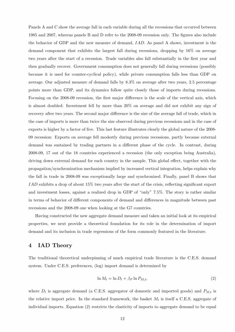
Figures 8 illustrates exactly how much of the fall in imports observed during 2008Q4 and 2009Q1

the three aggregate demand specifications are able to account for on average and for each individual

country (panel A and B refer to the panel regression (15) for all 18 countries, whereas panel C and D

to the same regression performed for the G7 only): The blue bar in the “Total” part of each diagram

shows the actual fall in aggregate imports in the 18 countries33 together with the predicted aggregate

fall using IAD (black bars), GDP (red bars), and DD (green bars), respectively. In particular, the

weighted average of real imports in our sample of countries fell by 5.6% in 2008Q4 and 9.3% in

2009Q1, on a quarterly basis. Using IAD as explanatory variable captures 67% and 63% of the fall

in aggregate imports in 2008Q4 and 2009Q1, respectively, while only 41% and 29% is explained by

the GDP-based specification. Results for the G7 are even more striking: On average, using IAD

explains 94% and 85% of the average fall in imports in the G7, against 61% and 51% when GDP is

used. In panel C and D, an additional (orange) bar is included for each country, corresponding to the

predictions of the IAD specification controlling also for changes in inventories.34 As shown by the

results of this exercise, which we do not show here for brevity, show very little change in the coefficient estimates andin sample fit of the IAD specification. (Details are available upon request.) This shows that the superiority of IADthat we document below relies on the ability of our new measure of demand to capture the dynamics of the differentdemand components and not on the time-variation of the aggregating weights.

31Notice that, in all specifications, we add two dummy variables to capture two episodes of erratic movements intrade in the UK in 2006Q1 and 2006Q3. Concerning these quarters the UK Office for National Statistics said: “Erraticand large movements in the level of trade associated with VAT Missing Trader Intra Community (MTIC) fraud havemade it especially difficult to interpret movements in imports and exports of goods.” The inclusion of such dummiesdoes not change the essence of the results.

32The U.S., the UK, Germany, France, Japan, Canada, Italy, and Spain. We do not report the results for the othercountries to save space, but they are available upon request.

33To construct the aggregate values of import growth, we used the respective average import shares of the countriesbetween 2000 and 2009.

34In particular, we estimate equation (15) using IAD as demand variable and adding as a control variable the changesin inventories as a percentage of GDP. For this exercise we used the time series of “change in stocks” and GDP atcurrent prices from the OECD Main Economic Indicator Database. The lack of long spans of data for some countries

20

orange bars, including changes in inventories helps improve the fit of the model: On average, using

IAD and controlling for changes in inventories explains 99% and 93% of the average fall in imports

in the G7 in 2008Q4 and 2009Q1, respectively.

The specification using IAD allows us to go one step further in investigating the relation between

the composition of demand and the GTC. Using the estimated coefficients from regression (15), we

can decompose import growth for each country in the panel and compute the individual contribution

of the four IAD components (C, I, X, and G), as well as PM , in explaining import fluctuations.

This allows us to disentangle, for instance, the relative importance of each demand component in

driving the fall in imports during the GTC.

Table 4 shows such a decomposition for 2009Q1, which corresponds to the trough in trade series

during the recent global crisis. The second column in the table reports quarterly import growth

in 2009Q1 for the 18 countries in the panel; Columns 3 to 8 report the percentage of the fall in

imports explained by the explanatory variables IAD and PM in equation (15) and by each demand

component in IAD (notice that the sum of the contributions of C, I, X, and G is equal to the

contribution of IAD). The last column shows the percentage of the fall in imports explained by

GDP from the regression using GDP as demand measure.

Several results are worth noting: First, the percentage of import growth explained by IAD

alone is in general very high, sometimes close to 100%, and, in most of the cases, much higher

than the percentage explained by GDP alone (in the cases of Germany and Sweden, however, both

specifications produce a larger-than-observed fall in imports, with the specification using GDP doing

slightly better than the IAD one). Second, the contribution of PM is negative for most of the

countries, meaning that relative import prices generally decreased in 2009Q1, hence, contributing an

increase rather than a decrease in imports over the same quarter (remember that the coefficient of

PM in Table 3 is negative).

Finally, looking at the individual demand components, two main facts emerge: First, private

and government consumption growth contribute only marginally to explaining the fall in imports in

2009Q1, the former explaining at most about 10% of it in a few countries, such as Denmark, the

UK, and the Netherlands, and the latter explaining an even lower percentage (and often implying an

increase rather than a decrease in imports as a result of the fact that government consumption was

increasing in most of the countries following the implementation of counter-cyclical fiscal policies).

Second, while investment and exports indeed explain most of the fall in imports, the main driver of

the fall varies substantially across countries, making it possible to identify countries that experienced

an “export-driven” or an “investment-driven” import collapse. The U.S., Norway, Sweden, and New

Zealand are among the countries that experienced an “investment-driven” import collapse, although

the percentage of the import fall explained by exports is also high for some of them. Japan, France,

in our sample makes it impossible to perform the same exercise for the entire panel of 18 countries. The results of thisexercise are not shown here for brevity, but they are available upon request.

21

Italy, Spain, Portugal, Belgium, Finland, and Korea instead experienced an “export-driven” import

collapse. Finally, in some countries, such as the UK, Canada, Germany, and the Netherlands, both

components of demand played roles of more similar magnitude in explaining the fall in imports.35

To summarize, according to our investigation, there is no major “puzzle” in the magnitude of

the fall in world trade observed during the recent financial crisis: Trade fell mostly because demand

crashed globally and did so particularly in its most import-intensive component—investment. More-

over, the strong relationship between exports and imports in each country, linked to the increased

internationalization of production and the strong dependence of the tradable sector on imported in-

puts, contributed to the simultaneity and unprecedented severity of the trade collapse. Our approach

and results confirm Marquez’s (1999) argument that using standard measures of aggregate demand,

such as GDP or domestic demand, in trade equations may be misleading, and more so in periods

in which the more import-intensive components of aggregate demand (i.e., investment and exports)

fluctuate much more than the others, such as the 2008-09 crisis.

5.3 Trade Elasticities over the Business Cycle: Toward a Solution to the Houthakker-

Magee Puzzle

Since the specification using IAD performs well in explaining the 2008-09 Great Trade Collapse, it

is important to understand whether the superiority of IAD against standard alternatives shown in

Table 3 comes from a better fit only during recession periods, when highly import-intensive demand

components tend to fall on average more than the components that are relatively less import-intensive

(as shown in Figure 6), or survives also when those periods are taken out of the sample. This is a

relevant question, since only in the second case we would be able to conclude that the new measure

of demand is in fact superior to standard measures and should be preferred in empirical work aimed

at estimating trade elasticities. Moreover, since not all recessions are crises and not all crises are

global, such as the 2008-09 one, we perform two alternative estimations for the recession periods,

one in which we exclude the recent global crisis and one where we include it.

This exercise also allows us to look more carefully at the values of the elasticity of imports to

aggregate demand over the business cycle, with an eye to addressing the well-known Houthakker-

Magee puzzle. In Section 4, we have provided a theoretical foundation for a (log) import demand

equation that is consistent with the traditional regression equation (14) (which, in turn, is the

foundation for regression (15) in the empirical literature), and does not restrict the elasticity of

imports to aggregate demand to be one. However, as discussed above, a demand system that does

not restrict the coefficient of aggregate demand in the import equation to one does not in itself imply

resolution of the economic puzzle that a coefficient significantly above one can derail sustainability.36

35Results for 2008Q4, which we do not show here to save space, are broadly similar and provide the same countryclassification.

36This represents a puzzle because it implies that, to prevent the trade balance from permanently moving intodeficit, the real exchange rate should permanently depreciate over time (this is also under the condition that foreign

22

Table 5 shows the result of the regressions (14) and (15) estimated separately for three different

data samples, one looking only at recessions and excluding the 2008-09 crisis, labeled as “recessions”

in the table, one looking at all recessions including the 2008-09 crisis, labeled as “GTC”, and one

looking only at “expansion” periods.37 We compare here the results from the equation using our

new import intensity-adjusted measure of demand and the specification using GDP, this latter being

in general the preferred measure in the literature estimating import elasticities. In the bottom panel

of Table 5, which shows results from regression equation (15), we report directly the sum of the

coefficients on contemporaneous and lagged aggregate demand to facilitate the comparison between

the two specifications. Several results are worth mentioning. First, both specifications do better at

estimating real import growth during recession times, i.e., in periods when the fall in demand is

particularly crucial to explain the behavior of trade. Second, the regression using IAD outperforms

the GDP one during both phases of the cycle in terms of goodness of fit—the improvement from

using IAD being even larger in the expansionary phases of the cycle. This shows that the results in

Table 3 are not driven only by extreme events, but they apply to the entire estimation period. Third,

the elasticity of imports to aggregate demand generally varies between recessions and expansions,

with some important distinctions to be made.

Starting with the results of “recessions” and “expansions” only (hence, excluding the GTC

episode): The import elasticity to GDP doubles during recessions and is close to 3 when one lag of

the exogenous variables is included in the regression. Instead, when IAD is used as aggregate de-

mand measure, the elasticity of imports to aggregate demand is remarkably stable across expansions

and recessions. It is exactly equal to one in the regression without lags and close to 1.5 when one

lag of IAD is added.38 These findings corroborate the idea that using GDP as demand measure

in trade equations may be misleading as it delivers highly volatile estimates of demand elasticities

that may indicate the presence of structural breaks even when this is not the case. Moreover, these

results suggest that the Houthakker-Magee puzzle, which is generally found in estimation of import

equations using GDP as measure of aggregate demand, may be driven by the inclusion of few but

highly volatile observations in the estimation sample, i.e., by the inclusion of recession episodes.39

Our new measure of demand, instead, by taking into account the different import contents of demand

components, delivers elasticities that are lower in magnitude and more stable over the cycle, making

a significant step toward the solution of the Houthakker-Magee puzzle.40

and domestic output grow at similar rates). Another puzzling implication of having a demand elasticity above one isthat output should be completely imported in the long run, barring a permanent depreciating trend.

37As in the previous section, recessions are defined as two consecutive quarters of negative real GDP growth. Wepresent results for the full set of countries. Results for the G7 are very similar and are available upon request.

38As a corollary, the IAD specification also provides higher (in absolute value) and more significant estimates forthe elasticities to import prices, which is a promising result as few papers find a large and significant role for relativeprices in trade equations.

39In their 1969 article, Houthakker and Magee use GNP at constant prices to compute import elasticities. Otherstudies have used either GNP or GDP to estimate the elasticity of imports to aggregate demand for the U.S. and otheradvanced economies (e.g., see Hooper, Johnson, and Marquez, 2000, and the literature reviewed therein).

40The empirical literature estimating import elasticities generally distinguishes between short-run and long-run elas-

23

Turning to the recession sample this time including the 2008-09 crisis, we observe an even stronger

increase of the elasticity of imports to GDP compared to expansionary phases—the contemporaneous

elasticity increases by a factor of 4 against a twofold increase when the GTC is excluded. In the case

of IAD, we also observe an increase of the import elasticity, although much lower than in the GDP

case, and a substantial increase of the in-sample fit. The increase in the elasticity estimates in both

specifications suggests that the 2008-09 global crisis was indeed an exceptional event. In particular,

results in Table 5 suggest that nonlinearities in the relation between imports and aggregate demand

still persist when IAD is used as measure of aggregate demand. This may be due to the role of other

factors not accounted for in our simple model of imports, such as financial constraints, the analysis

of which is beyond the scope of this paper. However, our simple model is enough to explain most

of the GTC episode, as shown in Section 5.2, and to reduce dramatically the elasticity difference

between different phases of the cycle.

To summarize, although a direct comparison with other models is not possible, the results using

IAD as demand variable go in the same direction of other papers that found lower import elastic-

ities to measures of aggregate demand once import equations are corrected for other factors, such

as vertical integration or aggregation bias. Cardarelli and Rebucci (2007), for instance, find that

once exports of intermediate products are added in the U.S. import equation to account for vertical

integration, the resulting GDP elasticity of imports drops significantly and becomes lower than one.

A similar result holds in Bussiere, Chudik, and Sestieri (2009) in the context of a global VAR where

exports enter in the import cointegration relation. Our approach is in principle more complete, as

we do not correct only for vertical integration, but also for the import content of different demand

components that is not taken into account when using GDP. Moreover, this approach has the advan-

tage of using a single statistic, the import intensity-adjusted measure of demand, delivering a single

demand coefficient of easier interpretation.

6 Conclusion

This paper proposed a new methodology for the estimation of trade elasticities, based on an import

intensity-adjusted measure of aggregate demand. While standard empirical trade models typically

use GDP (or domestic demand) as measure of aggregate demand, we argue that there is value added

in giving different weights to the components of GDP, which typically have very different import

intensities. In particular, the analysis of the new OECD Input-Output tables shows that, in general,

investment is significantly more import intensive than private consumption, which in turn is more

import intensive than government spending. In addition, we also find that exports are very import

intensive.

ticities, the latter generally preferred in debates on the sustainability of the current account to which the Houthakker-Magee puzzle is related. Here, we compute and discuss only short-run elasticities, the correct model specification toestimate long-run elasticities being beyond the scope of this paper.

24

Carefully disentangling the effects of investment, private and government consumption, and ex-

ports turns out to improve the goodness of fit of the model significantly, and it is especially important

in the context of the 2008-09 crisis, during which these different components of aggregate demand

evolved very differently. In particular, investment and exports decreased most significantly over this

period, whereas government spending remained robust, supported largely by the fiscal packages put

in place by governments in response to the crisis. Recognizing that investment and exports are more

import intensive than private and government consumption helps explain why regressions using stan-

dard measures of aggregate demand that do not account for differences in import intensity typically

underestimate the fall in trade that took place in 2008-09. Moreover, the high import intensity of ex-

ports contributes to explaining the synchronicity of the trade collapse across countries. We reported

key stylized facts on these developments, put also in historical perspective, and provided a theoret-

ical foundation and econometric evidence in support of our novel measure of demand. We showed

that using the import intensity-adjusted measure of demand proposed in this paper can significantly

enhance the performance of empirical trade models, helping resolve new and long-standing questions

in international economics.

25

References

Ahn, J, M. Amity, and D. E. Weinstein (2011): “Trade Finance and the Great Trade Collapse,”

American Economic Review Papers and Proceedings 101: 298-302.

Alessandria, G., J. P. Kaboski, and V. Midrigan (2010): “The Great Trade Collapse of 2008-09: An

Inventory Adjustment?,” IMF Economic Review 58: 254-294.

Amity, M., and D. E. Weinstein (2011): “Exports and Financial Shocks,” Quarterly Journal of

Economics.126: 1841-1877

Baldwin, R. (2009): “The Great Trade Collapse: Causes, Consequences and Prospects,” VoxEU.org

Ebook, November 27, 2009.

Bems, R., R. C. Johnson, and K.-M. Yi (2010): “Demand Spillovers and the Collapse of Trade in

the Global Recession,” IMF Economic Review 58: 295-326.

Benassy-Quere, A, Y. Decreux, L. Fontagne and D. Khoudour-Casteras (2009): “Economic Crisis

and Global Supply Chain,” CEPII Document de Travail 2009-15.

Bergin, P. R., and R. C. Feenstra (2000): “Staggered Price Setting and Endogenous Persistence,”

Journal of Monetary Economics 45: 657-680.

Bergin, P. R., and R. C. Feenstra (2001): “Pricing-to-Market, Staggered Contracts, and Real Ex-

change Rate Persistence,” Journal of International Economics 54: 333-359.

Bilbiie, F. O., F. Ghironi, and M. J. Melitz (2007): “Endogenous Entry, Product Variety, and

Business Cycles,” NBER Working Paper 13646.

Bussiere, M., A. Chudik, and G. Sestieri (2009): “Modeling Global Trade: Results from a GVAR

Model,” ECB Working Paper 1087.

Cardarelli, R., and A. Rebucci (2007): “Exchange Rates and the Adjustment of External Imbal-

ances,” in World Economic Outlook, Chapter 3, International Monetary Fund, April.

Chor, D., and K. Manova (2011): “Off the Cliff and Back? Credit Conditions and International

Trade during the Global Financial Crisis,” Journal of International Economics, forthcoming.

Corsetti, G., L. Dedola, and S. Leduc (2008): “International Risk-Sharing and the Transmission of

Productivity Shocks,” Review of Economic Studies 75: 443-473.

De Backer, K., and N. Yamano (2007): “The Measurement of Globalisation using International

Input-Output Tables,” OECD Science, Technology and Industry Working Paper 2007/8, OECD,

Directorate for Science, Technology and Industry.

26

Eaton, J., S. Kortum, B. Neiman, and J. Romalis (2011): “Trade and the Global Recession,” NBER

Working Paper 16666.

Erceg, C., L. Guerrieri, and C. Gust (2006): “Trade Adjustment and the Composition of Trade,”

International Finance Discussion Paper 2006-859, Board of Governors of the Federal Reserve System.

Feenstra, R. C. (1994): “New Product Varieties and the Measurement of International Prices,” The

American Economic Review 84: 157–77.

Feenstra, R. C. (2003a): Advanced International Trade: Theory and Evidence, Princeton Univer-

sity.Press, Princeton, NJ.

Feenstra, R. C. (2003b): “A Homothetic Utility Function for Monopolistic Competition Models,

without Constant Price Elasticity,” Economics Letters 78: 79-86.

Feenstra, R. C., Z. Li, and M. Yu. (2010): “Exports and Credit Constraints under Private Informa-

tion: Theory and Evidence from China,” NBER Working Paper 16940.

Ghironi, F., and M. J. Melitz (2005): “International Trade and Macroeconomic Dynamics with

Heterogeneous Firms,” Quarterly Journal of Economics 120: 865-915.

Guo, D., C. Webb, and N. Yamano (2009): “Towards Harmonised Bilateral Trade Data for Inter-

Country Input-Output Analyses: Statistical Issues,” OECD Science, Technology and Industry Work-

ing Paper 2009/4, OECD, Directorate for Science, Technology and Industry.

Harrigan, J. (1997): “Technology, Factor Supplies, and International Specialization: Estimating the

Neoclassical Model,” American Economic Review 87: 475-494.

Hooper, P., K. Johnson, and J. Marquez (2000): “Trade Elasticities for the G-7 Countries,” Princeton

Studies in International Economics 87.

Houthakker, H. S., and S. P. Magee (1969): “Income and Price Elasticities in World Trade,” Review

of Economics and Statistics 51: 111-125.

Hummels, D., J. Ishii, and K.-M. Yi, (2001): “The Nature and Growth of Vertical Specialization in

World Trade,” Journal of International Economics 54: 75–96.

International Monetary Fund (2010): World Economic Outlook, Chapter 4, “Do Financial Crises

Have Lasting Effects on Trade?,” October 2010.

Johnson, R.C., and G. Noguera (2011): “Accounting for Intermediates: Production Sharing and

Trade in Value Added,” Journal of International Economics, forthcoming.

Kee, H. L., A. Nicita, and M. Olarreaga (2008): “Import Demand Elasticities and Trade Distortions,”

Review of Economics and Statistics 90: 666-682.

27

Kohli, U. (1978): “A Gross National Product Function and the Derived Demand for Imports and

Supply of Exports,” Canadian Journal of Economics 11: 167-182.

Kohli, U. (1990a): “Price and Quantity Elasticities in U.S. Foreign Trade,” Economics Letters 33:

277-281.

Kohli, U. (1990b): “Growth Accounting in the Open Economy: Parametric and Nonparametric

Estimates,” Journal of Economic and Social Measurement 16: 125-136.

Kohli, U. (1993): “GNP Growth Accounting in the Open Economy: Parametric and Nonparametric

Estimates for Switzerland,” Swiss Journal of Economics and Statistics 129: 601-615.

Leibovici, F., and M. E. Waugh (2011): “International Trade and Intertemporal Substitution,” un-

published manuscript, New York University

Levchenko, A., L. Lewis, and L. Tesar (2010): “The Collapse of International Trade in 2008-9: In

Search of the Missing Gun,” IMF Economic Review 58: 214-253.

Levchenko, A., L. Lewis, and L. Tesar (2011): “The ‘Collapse in Quality’ Hypothesis,” American

Economic Review Papers and Proceedings 101: 293-297.

Mann, C. L., and K. Pluck (2005): “The U.S. Trade Deficit: A Disaggregated Perspective,” Working

Paper Series WP05-11, Peterson Institute for International Economics.

Marquez, J. R. (1999): “Long-Period Trade Elasticities for Canada, Japan, and the United States,”

Review of International Economics 7: 102–16.

Marquez, J. R. (2002): Estimating Trade Elasticities, Kluwer Academic Publisher, Dordrecht, The

Netherlands.

Organization for Economic Cooperation and Development (2011): OECD Science, Technology and

Industry Scoreboard 2011, http://dx.doi.org/10.1787/sti scoreboard-2011-en.

Rodrıguez-Lopez, J.-A. (2011): “Prices and Exchange Rates: A Theory of Disconnect,” Review of

Economic Studies 78: 1135-1177.

Sundararajan, V., and S. Thakur (1976): “Input-Output Approach to Import Demand Functions:

Experiments with Korean Data,” IMF Staff Papers 23: 674-698.

Yamano, N., and N. Ahmad (2006): “The OECD Input-Output Database: 2006 Edition,” OECD

Science, Technology and Industry Working Paper 2006/8, OECD, Directorate for Science, Technology

and Industry.

28

Figure 1: Recent developments and projections in world trade and output (volumes)

Source: IMF World Economic Outlook September 2011.

Figure 2: Growth rate of real imports in 2008Q4 and 2009Q1, q-o-q growth rates

Source: OECD Economic Outlook.

29

Figure 3: OECD Input-Output tables of Total, Domestic and Import transactions

Ind 1 Ind 2 PC GC GFCF Exports ImportsInd 1Ind 2VAOutput

Ind 1 Ind 2 PC GC GFCF Exports ImportsInd 1Ind 2ImportsVAOutput

Ind 1 Ind 2 PC GC GFCF Exports ImportsInd 1Ind 2PC : Private consumption by households, GC: Government consumption,GFCF: Gross fixed capital formation, VA: value addedAd = Zd/Output; Am = Zm/Output

TotalIntermediate Final demand

Domestic Intermediate Final demand

Import Intermediate Final demand

Zd

Zm

Fd

Fm

30

Figure 4: Import contents of main GDP components

Source: OECD OECD Input-Output Tables and authors�calculations.

Figure 5: Short-term correlations between imports and main GDP components

Source: OECD and authors�calculations.

31

Figure6:AveragebehaviourofGDPcomponentsduringrecessions(realvariables,cumulatedfall)

PanelA:Allcountries-1985-2007recessions

PanelB:Allcountries-2008-2009recessions

PanelC:G7-1985-2007recessions

PanelD:G7-2008-2009recessions

Source:OECDandauthors�calculations.

32

Figure 7: Actual vs. �tted values of real import growth - Selected economiesUnited States United Kingdom

Germany France

Japan Canada

Italy Spain

Notes: The solid line shows actual import growth, the dotted black line shows �tted values from the regression

using as a measure of demand, the dotted red line from the speci�cation and the dotted green line from

the domestic demand speci�cation, .

33

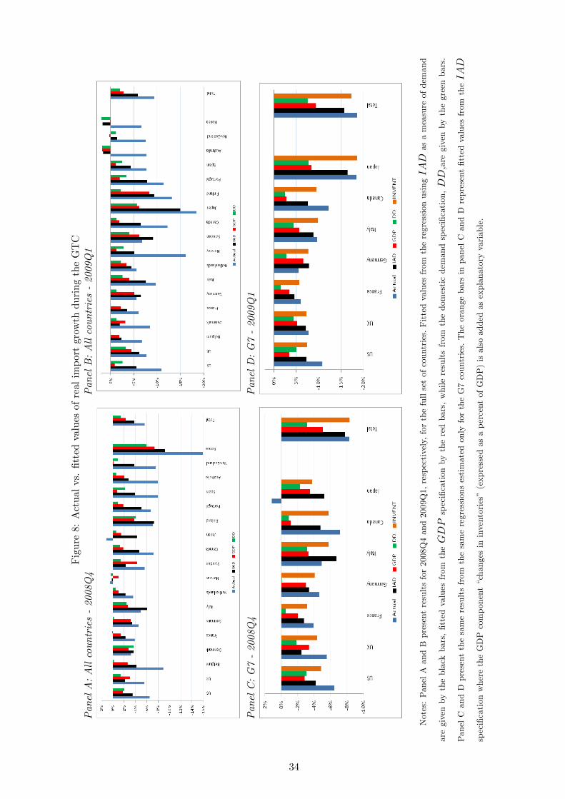
Figure8:Actualvs.�ttedvaluesofrealimportgrowthduringtheGTC

PanelA:Allcountries-2008Q4

PanelB:Allcountries-2009Q1

PanelC:G7-2008Q4

PanelD:G7-2009Q1

Notes:PanelAandBpresentresultsfor2008Q4and2009Q1,respectively,forthefullsetofcountries.Fittedvaluesfrom

theregressionusingasameasureofdemand

aregivenbytheblackbars,�ttedvaluesfrom

thespeci�cationbytheredbars,whileresultsfrom

thedomesticdemandspeci�cation,aregivenbythegreenbars.

PanelCandDpresentthesameresultsfrom

thesameregressionsestimatedonlyfortheG7countries.TheorangebarsinpanelCandDrepresent�ttedvaluesfrom

the

speci�cationwheretheGDPcomponent�changesininventories�(expressedasapercentofGDP)isalsoaddedasexplanatoryvariable.

34

Table 1.a: Total import content of main GDP components

1995 2000 2005 1995 2000 2005 1995 2000 2005 1995 2000 2005Australia 17,0% 18,6% 18,4% 9,0% 10,0% 9,9% 26,5% 26,6% 26,0% 14,0% 14,1% 14,0%Austria 24,2% 28,4% 28,7% 9,3% 11,0% 11,5% 36,7% 42,3% 42,7% 30,0% 34,6% 34,7%Belgium 32,3% 36,5% 33,6% 7,7% 10,6% 12,4% 43,6% 52,6% 49,7% 40,9% 45,9% 43,2%Canada 25,9% 23,7% 25,8% 10,3% 10,0% 9,8% 39,0% 42,1% 34,8% 30,5% 30,9% 27,4%Czech Republic 34,0% 39,5% 38,6% 18,8% 20,3% 19,8% 39,2% 53,3% 52,1% 29,1% 45,6% 48,3%Denmark 21,4% 30,3% 31,8% 7,1% 8,9% 10,4% 34,3% 40,3% 39,1% 27,1% 32,3% 34,9%Finland 20,6% 22,9% 26,8% 7,9% 10,8% 12,0% 42,4% 34,5% 32,4% 28,8% 33,4% 38,0%France 19,4% 22,0% 22,7% 8,2% 8,0% 8,7% 24,7% 27,2% 25,4% 19,8% 26,5% 27,0%Germany 18,3% 22,1% 22,6% 6,3% 8,0% 8,6% 22,7% 30,5% 31,1% 20,4% 25,8% 27,2%Greece 21,0% 24,4% 24,1% 11,6% 19,4% 9,9% 35,0% 36,5% 35,5% 15,8% 26,9% 25,9%Hungary 47,1% 35,4% 35,6% 29,2% 16,5% 15,4% 60,0% 53,6% 49,1% 47,4% 58,6% 55,8%Iceland 30,7% 16,9% 14,8% 17,4% 6,2% 5,5% 41,7% 24,1% 24,4% 26,7% 26,9% 27,1%Ireland 46,3% 42,0% 37,2% 16,4% 13,8% 14,4% 51,5% 48,6% 41,5% 48,7% 53,3% 50,7%Italy 18,2% 20,7% 21,3% 5,7% 6,7% 7,2% 25,7% 29,6% 27,3% 23,4% 27,1% 29,0%Japan 9,1% 9,8% 11,7% 3,0% 2,8% 6,0% 8,2% 10,6% 15,3% 8,4% 9,6% 15,4%Korea 21,4% 23,8% 24,2% 11,4% 10,2% 10,5% 30,8% 35,5% 28,9% 29,9% 38,1% 38,6%Luxembourg 45,5% 51,8% 50,3% 15,7% 18,1% 18,4% 49,9% 54,7% 53,6% 41,3% 57,7% 60,4%Mexico 31,4% 18,6% 17,2% 8,3% 5,0% 4,7% 42,6% 32,0% 30,2% 42,5% 39,3% 33,2%Netherlands 26,2% 28,5% 30,3% 10,4% 11,2% 11,3% 41,6% 41,6% 39,3% 33,3% 36,9% 34,9%New Zealand 21,1% 23,8% 21,4% 10,1% 11,6% 9,8% 37,9% 41,2% 39,3% 18,1% 19,2% 17,5%Norway 29,1% 31,8% 32,0% 11,1% 10,9% 10,9% 42,1% 42,0% 36,4% 21,6% 16,9% 16,2%Poland 19,7% 26,3% 24,9% 8,0% 6,4% 9,5% 30,0% 45,8% 47,9% 16,8% 24,7% 30,6%Portugal 27,5% 32,5% 29,0% 8,7% 10,9% 9,5% 35,3% 38,3% 36,1% 35,8% 30,8% 38,9%Slovak Republic 38,2% 43,1% 44,7% 17,7% 16,3% 21,6% 53,6% 52,2% 57,3% 35,4% 50,3% 48,6%Spain 18,1% 23,1% 24,0% 7,3% 9,9% 11,3% 26,1% 34,6% 28,3% 26,6% 33,9% 34,2%Sweden 23,2% 26,4% 28,1% 10,5% 11,3% 11,2% 43,7% 47,8% 43,0% 28,9% 32,3% 33,2%Switzerland 16,3% 22,5% 24,4% 5,8% 9,2% 9,3% 26,6% 33,1% 33,9% 14,2% 23,1% 25,3%Turkey 18,1% 15,8% 23,0% 6,0% 10,3% 14,6% 36,8% 33,7% 41,7% 13,9% 13,6% 30,7%United Kingdom 21,1% 24,9% 27,2% 11,2% 12,7% 12,5% 37,4% 35,0% 25,4% 22,2% 20,3% 18,6%United States 8,7% 10,5% 11,9% 3,7% 6,0% 6,2% 18,4% 19,1% 17,3% 9,5% 11,0% 12,3%Argentina 8,2% 7,9% 12,4% 2,2% 1,8% 2,8% 22,6% 22,6% 27,1% 10,3% 10,9% 16,8%Brazil 9,6% 12,2% 10,4% 3,3% 4,8% 3,7% 13,1% 14,6% 20,9% 10,8% 12,0% 14,4%China 11,4% 13,4% 19,1% 9,9% 10,8% 13,8% 26,2% 20,8% 28,8% 15,5% 19,6% 27,4%Chinese Taipei 24,4% 22,9% 26,3% 13,6% 9,3% 8,7% 42,0% 49,9% 50,6% 35,2% 37,3% 48,3%India 7,6% 10,4% 14,0% 5,9% 8,1% 8,3% 21,6% 23,7% 28,7% 10,4% 12,4% 18,5%Indonesia 16,9% 23,3% 22,4% 12,4% 14,0% 13,9% 30,6% 35,5% 30,4% 15,1% 19,5% 18,1%Israel 20,1% 30,2% 29,6% 6,2% 14,9% 15,5% 21,4% 38,3% 39,5% 16,6% 34,1% 37,9%Russian Fed. 22,8% 24,7% 23,2% 10,6% 12,1% 12,2% 20,0% 25,7% 26,0% 10,6% 10,9% 9,1%Singapore 45,9% 43,0% 46,7% 27,6% 35,0% 35,4% 58,2% 59,0% 64,0% 57,2% 58,4% 56,6%South Africa 14,3% 18,4% 20,6% 5,5% 7,1% 8,7% 29,5% 37,4% 34,5% 9,7% 15,2% 14,6%Hong Kong 12,0% 9,5% 7,0% 8,4% 9,7% 6,3% 14,0% 10,2% 5,9% 13,9% 14,1% 12,6%Chile 23,4% 27,8% 31,7% 8,5% 8,2% 9,8% 39,4% 35,2% 37,6% 19,0% 19,0% 23,2%Estonia 49,8% 40,0% 41,3% 25,1% 19,1% 18,5% 69,2% 58,8% 55,5% 47,5% 55,1% 50,8%Slovenia 39,0% 36,2% 37,6% 19,6% 16,3% 15,7% 54,2% 54,7% 50,6% 36,9% 43,6% 45,6%Malaysia 46,7% 41,8% 42,3% 24,4% 24,4% 25,2% 55,9% 64,1% 62,3% 38,8% 53,0% 50,4%Philippines 25,1% 28,5% 32,1% 12,0% 11,8% 8,3% 41,2% 52,3% 53,1% 32,4% 46,0% 41,6%Thailand 28,9% 31,7% 26,9% 8,2% 9,7% 10,5% 42,3% 52,5% 61,8% 33,5% 40,6% 38,1%Romania 22,4% 24,1% 26,9% 19,0% 20,8% 17,8% 35,8% 47,9% 51,7% 26,0% 27,9% 29,0%Vietnam 16,3% 33,3% 36,9% 12,2% 26,3% 28,8% 40,5% 50,6% 54,3% 15,0% 27,5% 30,6%Saudi Arabia 17,4% 30,5% 34,8% 12,7% 18,8% 14,2% 19,6% 48,4% 52,6% 1,3% 5,9% 2,0%

Import content of exports.

Import content of privateconsumption

Import content of governmentconsumption

Import content of totalinvestment

Source: OECD Input-Output Tables and authors�calculations.

35

Table 1.b: Induced import content of main GDP components

1995 2000 2005 1995 2000 2005 1995 2000 2005Australia 9,1% 9,1% 8,8% 9,0% 8,9% 8,7% 11,1% 11,1% 11,1%Austria 11,0% 13,3% 13,8% 7,8% 9,1% 9,2% 16,2% 16,0% 18,1%Belgium 17,4% 19,5% 18,9% 7,3% 9,5% 11,2% 21,6% 23,8% 21,0%Canada 11,3% 10,6% 9,4% 10,3% 10,0% 9,8% 16,1% 15,3% 15,6%Czech Republic 19,1% 20,6% 20,5% 14,2% 17,6% 14,4% 21,0% 23,9% 20,9%Denmark 9,9% 11,7% 13,3% 6,4% 8,1% 9,3% 15,3% 17,5% 19,0%Finland 10,7% 12,7% 13,3% 7,1% 9,8% 10,8% 12,3% 18,4% 18,4%France 9,3% 11,0% 10,7% 6,5% 6,8% 6,8% 12,1% 13,5% 13,0%Germany 9,0% 11,7% 12,0% 5,5% 7,0% 7,1% 11,7% 14,5% 15,4%Greece 8,8% 11,3% 10,0% 10,6% 18,1% 10,2% 17,0% 14,0% 13,8%Hungary 25,6% 23,7% 18,5% 19,5% 13,5% 11,4% 22,3% 20,8% 20,7%Iceland 14,8% 9,2% 8,0% 13,7% 6,2% 5,5% 13,2% 5,4% 5,7%Ireland 16,3% 16,1% 19,6% 13,1% 13,8% 14,4% 23,0% 21,7% 22,8%Italy 11,8% 13,2% 13,1% 5,4% 6,2% 6,6% 14,7% 15,6% 14,8%Japan 4,6% 5,1% 6,9% 3,0% 2,8% 6,0% 5,6% 6,4% 9,1%Korea 14,8% 16,6% 16,0% 11,4% 10,2% 10,5% 15,4% 17,8% 17,8%Luxembourg 15,4% 18,8% 22,1% 13,0% 15,8% 16,7% 19,3% 22,1% 30,8%Mexico 18,0% 11,7% 11,2% 8,3% 5,0% 4,6% 26,8% 16,2% 14,4%Netherlands 13,8% 14,5% 15,8% 9,2% 10,0% 10,3% 19,7% 19,0% 16,3%New Zealand 11,5% 12,6% 11,0% 8,8% 10,4% 8,9% 14,4% 15,3% 13,5%Norway 13,2% 12,8% 11,9% 10,0% 9,5% 9,3% 15,0% 14,2% 14,1%Poland 12,2% 14,3% 14,8% 6,9% 6,0% 7,8% 15,0% 14,3% 15,9%Portugal 14,6% 15,2% 14,7% 7,7% 8,3% 7,9% 16,0% 16,4% 17,0%Slovak Republic 18,8% 20,7% 17,5% 17,7% 16,3% 12,7% 18,7% 21,9% 18,2%Spain 10,7% 12,8% 12,2% 6,7% 8,8% 9,0% 12,7% 15,6% 14,0%Sweden 12,6% 14,1% 14,7% 9,5% 10,0% 9,6% 15,7% 15,9% 17,2%Switzerland 8,3% 11,0% 13,2% 5,8% 9,1% 9,2% 11,0% 17,5% 18,3%Turkey 9,6% 11,6% 14,5% 6,0% 6,8% 10,7% 11,0% 13,0% 21,0%United Kingdom 11,7% 10,4% 10,5% 11,2% 12,3% 12,5% 12,2% 11,7% 11,4%United States 4,1% 4,6% 5,8% 3,7% 4,5% 6,2% 7,8% 7,8% 9,0%Argentina 4,9% 4,5% 6,3% 2,2% 1,8% 2,8% 7,1% 7,1% 11,6%Brazil 5,7% 7,2% 7,1% 3,3% 4,8% 3,7% 5,9% 7,7% 11,0%China 9,6% 10,3% 14,0% 9,5% 10,6% 13,6% 11,5% 15,4% 20,5%Chinese Taipei 12,9% 11,9% 15,4% 13,6% 9,3% 8,7% 18,9% 18,4% 21,0%India 5,5% 6,4% 11,4% 4,2% 4,4% 8,3% 12,1% 13,3% 19,9%Indonesia 9,7% 11,2% 12,2% 9,8% 12,0% 12,1% 18,1% 21,8% 19,8%Israel 9,1% 14,8% 15,0% 6,2% 14,9% 15,5% 11,3% 19,3% 20,6%Russian Fed. 8,9% 9,5% 9,3% 9,9% 11,7% 11,7% 10,8% 13,2% 13,5%Singapore 17,4% 18,7% 20,3% 27,6% 35,0% 35,4% 20,5% 23,3% 25,4%South Africa 7,6% 10,4% 11,0% 5,5% 7,1% 8,7% 10,0% 13,4% 16,1%Hong Kong 7,0% 5,7% 4,5% 8,4% 9,7% 6,3% 7,3% 4,9% 2,3%Chile 12,9% 15,7% 17,3% 8,5% 8,2% 9,8% 12,0% 12,3% 14,7%Estonia 23,3% 19,6% 18,7% 16,7% 17,3% 16,2% 19,1% 21,5% 20,6%Slovenia 14,7% 14,3% 13,9% 16,1% 12,4% 11,6% 18,7% 18,3% 19,7%Malaysia 20,8% 21,9% 23,3% 13,1% 22,2% 22,4% 20,0% 21,8% 19,9%Philippines 14,6% 15,2% 15,6% 12,0% 11,8% 8,3% 17,1% 16,9% 17,6%Thailand 15,3% 17,3% 21,8% 5,8% 9,7% 10,1% 19,9% 20,1% 25,3%Romania 12,2% 15,7% 17,2% 18,0% 20,8% 17,8% 18,4% 15,4% 14,0%Vietnam 12,3% 21,5% 23,9% 12,2% 26,3% 28,8% 27,6% 37,6% 41,4%Saudi Arabia 3,7% 7,0% 8,3% 7,3% 11,9% 6,7% 2,4% 9,9% 11,9%

Import content of privateconsumption

Import content of governmentconsumption

Import content of totalinvestment

Source: OECD Input-Output Tables and authors�calculations.

36

Table 1.c: Direct import content of main GDP components

1995 2000 2005 1995 2000 2005 1995 2000 2005Australia 7,9% 9,5% 9,6% 0,0% 1,0% 1,2% 15,4% 15,5% 15%Austria 13,2% 15,1% 14,9% 1,4% 1,9% 2,2% 20,5% 26,3% 25%Belgium 14,8% 17,0% 14,8% 0,5% 1,1% 1,2% 22,0% 28,7% 29%Canada 14,6% 13,2% 16,4% 0,0% 0,0% 0,0% 22,9% 26,8% 19%Czech Republic 15,0% 19,0% 18,1% 4,6% 2,6% 5,4% 18,1% 29,4% 31%Denmark 11,5% 18,6% 18,5% 0,7% 0,9% 1,1% 18,9% 22,9% 20%Finland 9,9% 10,1% 13,6% 0,8% 1,0% 1,2% 30,1% 16,1% 14%France 10,1% 11,0% 12,0% 1,7% 1,2% 1,9% 12,6% 13,7% 12%Germany 9,3% 10,3% 10,5% 0,8% 1,0% 1,5% 11,0% 16,1% 16%Greece 12,2% 13,1% 14,1% 1,0% 1,3% ­0,3% 18,0% 22,4% 22%Hungary 21,5% 11,7% 17,0% 9,7% 3,0% 4,1% 37,7% 32,8% 28%Iceland 15,9% 7,7% 6,8% 3,7% 0,0% 0,0% 28,5% 18,7% 19%Ireland 30,0% 25,9% 17,6% 3,3% 0,0% 0,0% 28,5% 26,9% 19%Italy 6,4% 7,5% 8,1% 0,3% 0,5% 0,6% 11,0% 14,0% 13%Japan 4,5% 4,7% 4,8% 0,0% 0,0% 0,0% 2,6% 4,3% 6%Korea 6,6% 7,2% 8,2% 0,0% 0,0% 0,0% 15,4% 17,7% 11%Luxembourg 30,1% 33,0% 28,1% 2,6% 2,2% 1,7% 30,6% 32,7% 23%Mexico 13,4% 6,9% 6,0% 0,1% 0,1% 0,0% 15,8% 15,8% 16%Netherlands 12,3% 14,1% 14,6% 1,2% 1,2% 0,9% 21,9% 22,7% 23%New Zealand 9,6% 11,2% 10,4% 1,3% 1,2% 0,9% 23,6% 25,9% 26%Norway 15,8% 19,1% 20,1% 1,1% 1,5% 1,6% 27,1% 27,8% 22%Poland 7,5% 12,0% 10,1% 1,0% 0,4% 1,7% 15,0% 31,5% 32%Portugal 13,0% 17,3% 14,4% 0,9% 2,6% 1,6% 19,3% 21,9% 19%Slovak Republic 19,4% 22,4% 27,2% 0,0% 0,0% 8,9% 34,9% 30,3% 39%Spain 7,4% 10,3% 11,8% 0,6% 1,1% 2,4% 13,5% 19,0% 14%Sweden 10,6% 12,4% 13,5% 1,0% 1,3% 1,6% 28,0% 31,9% 26%Switzerland 8,0% 11,5% 11,2% 0,1% 0,1% 0,1% 15,6% 15,6% 16%Turkey 8,5% 4,2% 8,4% 0,0% 3,4% 3,9% 25,8% 20,7% 21%United Kingdom 9,4% 14,5% 16,7% 0,0% 0,4% 0,0% 25,2% 23,4% 14%United States 4,5% 6,0% 6,0% 0,0% 1,5% 0,0% 10,6% 11,4% 8%Argentina 3,3% 3,4% 6,1% 0,0% 0,0% 0,0% 15,5% 15,5% 15%Brazil 3,9% 5,1% 3,3% 0,0% 0,0% 0,0% 7,2% 6,9% 10%China 1,8% 3,1% 5,1% 0,4% 0,2% 0,2% 14,7% 5,4% 8%Chinese Taipei 11,5% 11,0% 10,8% 0,0% 0,0% 0,0% 23,1% 31,5% 30%India 2,1% 4,0% 2,6% 1,7% 3,7% 0,0% 9,5% 10,4% 9%Indonesia 7,3% 12,1% 10,2% 2,6% 2,0% 1,8% 12,4% 13,7% 11%Israel 11,0% 15,4% 14,6% 0,0% 0,0% 0,0% 10,1% 19,0% 19%Russian Fed. 13,9% 15,2% 13,9% 0,7% 0,4% 0,4% 9,2% 12,5% 12%Singapore 28,4% 24,3% 26,3% 0,0% 0,0% 0,0% 37,7% 35,8% 39%South Africa 6,7% 8,0% 9,5% 0,0% 0,0% 0,0% 19,5% 24,1% 18%Hong Kong 4,9% 3,8% 2,5% 0,0% 0,0% 0,0% 6,6% 5,3% 4%Chile 10,5% 12,1% 14,4% 0,0% 0,0% 0,0% 27,4% 22,8% 23%Estonia 26,4% 20,5% 22,6% 8,5% 1,9% 2,3% 50,1% 37,4% 35%Slovenia 24,3% 21,9% 23,7% 3,5% 4,0% 4,1% 35,5% 36,3% 31%Malaysia 25,9% 19,9% 19,0% 11,3% 2,2% 2,8% 35,9% 42,3% 42%Philippines 10,5% 13,3% 16,5% 0,0% 0,0% 0,0% 24,0% 35,5% 35%Thailand 13,5% 14,4% 5,1% 2,4% 0,0% 0,5% 22,4% 32,3% 36%Romania 10,1% 8,5% 9,7% 0,9% 0,0% 0,0% 17,5% 32,5% 38%Vietnam 4,0% 11,8% 13,0% 0,0% 0,0% 0,0% 12,9% 12,9% 13%Saudi Arabia 13,7% 23,5% 26,5% 5,4% 6,9% 7,4% 17,2% 38,6% 41%

Import content of privateconsumption

Import content of governmentconsumption

Import content of totalinvestment

Source: OECD Input-Output Tables and authors�calculations.

37

Tab

le2.

DescriptiveStatistics

Thetable

presents

descriptivestatisticsforthelogdifferen

ceofGDP,IAD

andim

ports,M

,where∆

den

otesfirstdifferen

ces.

Themeansandstandard

deviationsare

reported

inpercentunits.ρ(Q

)is

thecontemporaneouscorrelationcoeffi

cien

tbetweeneach

ofoftheva

riablesin

columnandtheva

riable∆ln

Q,whereQ

=IAD,G

DP,or

M.Thedata

setcoversquarterly

data

from

1985Q1to

2010Q2.

Allcountries

Ful lsample

Recession

sExpansion

s

∆lnIAD

∆lnGDP

∆ln

M∆ln

IAD

∆ln

GDP

∆ln

M∆ln

IAD

∆ln

GDP

∆lnM

Mean

0.81

0.62

1.33

−1.49

−0.89

−2.06

1.08

0.79

1.74

Sd

1.71

1.02

3.24

2.08

1.02

4.28

1.45

0.87

2.84

ρ(IAD)

1.00

1.00

1.00

ρ(G

DP)

0.66

1.00

0.73

1.00

0.53

1.00

ρ(M

)0.62

0.42

1.00

0.74

0.63

1.00

0.50

0.24

1.00

#Observation

s1836

1836

1836

190

190

190

1646

1646

1646

G7

∆lnIAD

∆lnGDP

∆ln

M∆ln

IAD

∆ln

GDP

∆ln

M∆ln

IAD

∆ln

GDP

∆lnM

Mean

0.67

0.51

1.17

−1.55

−0.83

−2.11

0.93

0.67

1.59

Sd

1.37

0.78

2.59

2.04

0.84

3.55

0.96

0.59

2.12

ρ(IAD)

1.00

1.00

1.00

ρ(G

DP)

0.77

1.00

0.85

1.00

0.60

1.00

ρ(M

)0.70

0.48

1.00

0.80

0.62

1.00

0.53

0.21

1.00

#Observation

s714

714

714

7676

76

638

638

638

38

Table 3: Panel Results

The table reports in-sample estimates of panel regressions of the form (15) performed on our set of 18 countries

and on the G7 countries, respectively. The dependent variable is the quarterly growth rate of real imports of goods

and services. Three models are compared in the table, according to the demand measure D used in each regression,

where IAD stands for our new import intensity-adjusted measure of demand, GDP for real GDP, and DD for

real domestic demand. PM are relative import prices. To save space we do not report here the point estimates of the

constant, and of the lagged values of the dependent variable and PM . R2 is the in-sample coefficient of determination.

Robust standard errors are reported in parentheses. ∗, ∗∗, and ∗∗∗ indicate significance at the 10%, 5%, and 1% levels,

respectively. The analysis uses quarterly data from 1985Q1 to 2010Q2.

All countries

IAD specification GDP specification DD specification

0 lags 1 lag 0 lags 1 lag 0 lags 1 lag

∆ln(D)t 1.18*** 1.22*** 1.34*** 1.33*** 1.48*** 1.55***

(0.0978) (0.0711) (0.2872) (0.2423) (0.1393) (0.0827)

∆ln(D)t−1 0.50*** 0.88*** 0.58***

(0.0483) (0.1376) (0.1280)

∆ln(PM )t -0.17*** -0.18*** -0.14* -0.15** -0.05 -0.07

(0.05564) (0.0477) (0.0721) (0.0615) (0.0736) (0.0609)

R-sq 0.40 0.46 0.19 0.26 0.26 0.30

#Observations 1836 1836 1836 1836 1836 1836

G7

IAD specification GDP specification DD specification

0 lags 1 lag 0 lags 1 lag 0 lags 1 lag

∆ ln(D)t 1.35*** 1.26*** 1.60*** 1.27*** 1.62*** 1.50***

(0.1021) (0.0851) (0.1996) (0.1221) (0.2292) (0.1617)

∆ ln(D)t−1 0.47*** 0.90*** 0.63***

(0.1096) (0.1884) (0.1509)

∆ ln(PM )t -0.11** -0.14*** -0.01 -0.04 0.09 0.03

(0.0371) (0.0340) (0.0540) (0.0375) (0.0469) (0.0478)

R-sq 0.51 0.54 0.25 0.32 0.27 0.32

#Observations 714 714 714 714 714 714

39

Table 4. Import Growth Decomposition - 2009Q1

The second column reports quarterly import growth in 2009Q1 for the 18 countries in our panel; Columns 3 to 8

report the percentage of import growth explained by the explanatory variables IAD and PM in equation (15) and

by each demand component in IAD (notice that the sum of the contributions of C , X , I and G is equal to the

contribution of IAD). The last column shows the percentage of import growth explained by GDP . Negative values

indicate that the explanatory variable account for import growth in the opposite direction of the one observed.

Percentage of import growth explained by :

Import Growth (%) IAD C X I G PM GDP

U.S. −10.9 80.6 1.4 31.4 47.7 0.2 −13.0 30.0

UK −7.7 93.2 9.8 37.0 46.3 0.1 5.7 65.8

Japan −18.5 93.1 2.7 73.9 17.5 −0.9 −11.9 44.8

Germany −5.5 158.9 −1.0 94.8 68.2 −3.1 −16.0 122.7

France −6.0 89.8 −0.5 70.5 21.7 −1.9 −9.6 58.1

Italy −9.7 103.9 4.4 69.8 29.7 0.0 −10.9 59.8

Canada −12.2 70.3 1.5 31.5 38.5 −1.2 −1.8 26.1

Australia −7.7 11.9 −1.7 −4.7 18.9 −0.6 −5.1 −4.3

Spain −7.6 95.2 7.8 54.1 36.2 −2.8 −10.5 41.3

Netherlands −5.6 101.9 8.9 53.6 41.8 −2.5 −3.8 76.6

Porugal −11.4 90.5 6.0 51.5 35.1 −2.1 −5.0 32.1

Norway −16.2 27.3 3.0 3.4 23.4 −2.5 4.0 4.4

NewZealand −7.5 57.1 4.5 2.0 51.9 −1.3 −10.6 20.6

Sweden −6.8 158.6 2.9 48.8 109.3 −2.6 −1.0 108.2

Belgium −6.7 86.6 3.7 61.1 21.7 0.1 −16.5 63.1

Finland −13.1 97.3 3.5 69.5 25.3 −1.0 −11.2 82.4

Denmark −8.5 44.9 12.2 27.7 6.7 −1.8 −9.5 53.1

Korea −6.7 63.7 7.2 50.2 13.1 −6.7 −26.7 56.7

40

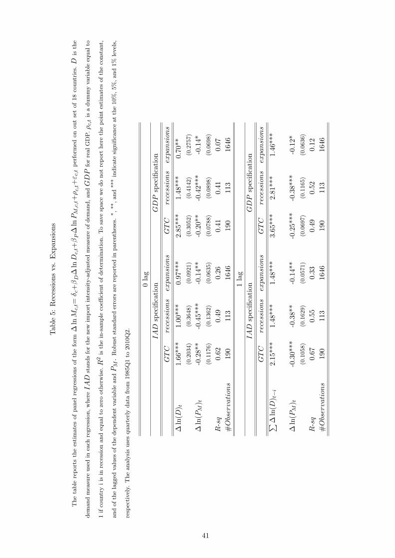
Tab

le5:

Recession

svs.

Expan

sion

s

Thetable

reportstheestimatesofpanel

regressionsoftheform

∆lnM

c,t=

δ c+βD∆ln

Dc,t+

βP∆ln

PM

,c,t+ρc,t+

ε c,t

perform

edonoutsetof18countries.D

isthe

dem

andmeasure

usedin

each

regression,whereIAD

standsforthenew

import

intensity-adjusted

measure

ofdem

and,andGDP

forrealGDP.ρc,tisadummyva

riable

equalto

1ifcountryiis

inrecessionandequalto

zero

otherwise.R

2is

thein-sample

coeffi

cien

tofdetermination.Tosavespace

wedonotreport

herethepointestimatesoftheconstant,

andofthelagged

values

ofthedep

enden

tva

riable

andPM.Robust

standard

errors

are

reported

inparentheses.∗ ,

∗∗,and∗∗

∗indicate

significance

atthe10%,5%,and1%

levels,

resp

ectively.

Theanalysisusesquarterly

data

from

1985Q1to

2010Q2.

0lag

IAD

specification

GDP

specification

GTC

recessions

expansion

sGTC

recessions

expansion

s

∆ln(D

) t1.66***

1.00***

0.97***

2.85**

*1.48***

0.70**

(0.2034)

(0.3648)

(0.0921)

(0.3052)

(0.4142)

(0.2757)

∆ln(P

M) t

-0.28**

-0.45***

-0.14**

-0.20**

-0.42***

-0.14*

(0.1176)

(0.1362)

(0.0635)

(0.0788)

(0.0898)

(0.0698)

R-sq

0.62

0.49

0.26

0.41

0.41

0.07

#Observation

s190

113

1646

190

113

1646

1lag

IAD

specification

GDP

specification

GTC

recessions

expansion

sGTC

recessions

expansion

s∑ ∆

ln(D

) t−i

2.15***

1.48***

1.48***

3.65**

*2.81***

1.46***

∆ln(P

M) t

-0.30***

-0.38**

-0.14**

-0.25***

-0.38***

-0.12*

(0.1058)

(0.1629)

(0.0571)

(0.0697)

(0.1165)

(0.0636)

R-sq

0.67

0.55

0.33

0.49

0.52

0.12

#Observation

s190

113

1646

190

113

1646

41