Estimating Economic Impacts of the U.S.-South Korea Free Trade Agreement*

Dan Wei

Sol Price School of Public Policy University of Southern California

100D University Gateway Los Angeles, CA 90089

(213) 740-0034 danwei@usc.edu

Zhenhua Chen

Knowlton School of Architecture The Ohio State University

295 Knowlton Hall, 275 W. Woodruff Ave. Columbus, OH 43210

(614) 688-2841 chen.7172@osu.edu

Adam Rose

Sol Price School of Public Policy University of Southern California

RGL 230, 650 Childs Way Los Angeles, CA 90089

(213) 740-8022 adam.rose@usc.edu

March 14, 2018

*The authors are, respectively, Research Assistant Professor, Price School of Public Policy, and Faculty Affiliate, Center for Risk and Economic Analysis of Terrorism Events (CREATE), University of Southern California (USC); Assistant Professor, Knowlton School of Architecture, The Ohio State University; Research Professor, Price School, and Faculty Affiliate, CREATE, USC. The research contained in this paper was supported by the United States Department of Homeland Security (DHS) Customs and Border Protection (CBP) under Grant No. BOA HSHQDC-10-A-BOA19 through the National Center for Risk and Economic Analysis of Terrorism Events (CREATE). We are grateful to the following people for commenting on the earlier drafts of the study: Bryan Roberts, Katie Foreman, Gia Harrigan, and staff of CBP. We also thank Brett Shears for his valuable research assistance. However, the views contained in the paper are solely those of the authors and not necessarily of any of the institutions with which they are affiliated nor the institutions that funded the research.

Estimating Economic Impacts of the U.S.-South Korea Free Trade Agreement

Abstract

We analyze the economic impacts of the United States-South Korea Free Trade Agreement by

applying the Global Trade Analysis Project (GTAP) computable general equilibrium model to

highly disaggregated commodity flow data. The analysis calculates the impacts in terms of

welfare effects, national economic indicators (such as GDP), and business performance metrics

(such as profits or sales revenue), which can be used by a variety of decision-makers. Our

results suggest several trade-offs among these measures. Positive welfare gains between the

US and South Korea are about the same in absolute terms, but favor the latter in relative terms,

and very heavily so for GDP gains. Moreover, the US is projected to incur a loss of gross output

(sales revenue) in several major manufacturing sectors that are heavily concentrated in

geographic areas that have been promised a return of jobs by the new Administration.

Keywords: Free Trade Agreement; United States; South Korea; Tariff Barriers; Computable

General Equilibrium Modeling; GTAP

1

ESTIMATING ECONOMIC IMPACTS OF THE U.S.-SOUTH KOREA FREE TRADE AGREEMENT

I. INTRODUCTION

A free trade agreement (FTA) refers to a treaty established between two or more countries in

order to reduce the trade barriers between them. Trade barriers, such as import tariffs, trade

quotas, and import/export licenses and standards, are government established restrictions on

international trade with the aims to protect domestic production and employment, tackle

unfair trade practices (such as dumping), protect domestic infant industry, and ensure national

security (Elwell, 2006). A FTA usually removes most of these trade barriers in order to improve

overall economic efficiency.

As of January 2015, the U.S. had 14 FTAs in force with 20 countries (CBP, 2014). In addition, the

Trans-Pacific Partnership (TPP) among 12 Pacific Rim countries (including Australia, Brunei

Darussalam, Canada, Chile, Japan, Malaysia, Mexico, New Zealand, Peru, Singapore, Vietnam,

and U.S.) reached an agreement in October, 2015. The U.S. is also negotiating with the

European Union on the Trans-Atlantic Trade and Investment Partnership (ITA, 2015).

However, all these trade agreements are facing great uncertainties due to the inauguration of

the new U.S. President, Donald Trump. According to the Trump Administration, U.S. trade

policies will be renegotiated or reconsidered with the intent of creating American jobs,

increasing American wages, and reducing America’s trade deficit.1 It is clear that the existing

FTAs will be under increased scrutiny by the new Administration. In fact, Trump signed an

1 Donald J. Trump for President, Inc. (2017).

2

Executive Order withdrawing the U.S. from the TPP immediately after he was sworn in as the

President in January 2017. It is therefore important to reassess the economic impacts of the

existing trade policies including FTAs to provide a better understanding of the issues in order to

inform the policy debate. Most economic analyses in recent years have focused on the impacts

of these agreements in terms of welfare effects, considered to be the best measure for

evaluating policies, because they are comprehensive and focus on changes in the well-being of

the aggregate of individuals in a society (see, e.g., Dixon and Rimmer, 2005; Burfisher, 2011).

However, the current policy climate is likely to renew attention to other metrics. This includes

national economic indicators, such as GDP, which are less arcane to policymakers and thus

more likely to be the focus of attention by executive and legislative branch decision-makers.

On the other hand, industry executives and stock market analysts are likely to be more

interested in measures of business performance such as profits, sales revenue and market

share.

In this study, we evaluate the economic impacts of FTA with considerations of all three of these

metrics for the United States-South Korea FTA (US-Korea FTA). Specifically, our assessment is

conducted in two steps. In the first step, the direct benefits of the US-Korea FTA are

summarized, including the benefits of tariff reduction or elimination policies, as well as the

benefits from reduction or removal of non-tariff barriers. In the second step, we present the

methodology to analyze the indirect effects of tariff reduction or elimination using the Global

Trade Analysis Project (GTAP) computable general equilibrium (CGE) model. Our paper

advances the literature on the US-Korea FTA by analyzing both standard welfare measures and

broader economic indicators, and by utilizing the most detailed commodity data available. We

3

decompose welfare effects into three components (allocation, commodity terms of trade, and

investment-savings terms of trade effects) and present the macroeconomic impacts in terms of

three indicators (GDP, gross output and imports). Both the tariff elimination phase-in schedule

and import and export data are specified at the 10-digit Harmonized Tariff Schedule (HTS) level

in order to calculate the actual (ex post) percentage tariff reduction of each individual

commodity as of 2014. In contrast, earlier literature on the economic impacts of the US-Korea

FTA have been based on various assumed tariff elimination schedules (see, e.g., Cheong and

Wang, 1999; McDaniel and Fox, 2001; Choi and Schott, 2005; Lee and Lee, 2005; Schott et al.,

2006), some of which are discussed in more detail below.

Our analysis indicates that the US-Korea FTA generates a divergence of outcomes. From the

standpoint of the US, welfare gains are estimated to be $368 million, GDP gains are estimated

to be $45 million, and total gross output (sales revenue) is estimated to incur a net loss of $143

million. Moreover, 34 out of 57 sectors of the US economy are estimated to incur gross output

losses. This includes three advanced manufacturing sectors estimated to incur gross output

reductions in excess of $175 million each. Ironically, the sectors that are estimated to gain the

most are agriculture, mining, construction, and primary manufacturing. These results indicate

the continued shift in comparative advantage away from US manufacturing with respect to

rising economies such as that of South Korea. Note that the previous estimates of aggregate

welfare gains are typically much higher than ours for both countries because most of prior

studies focused on 100% tariff removal. Thus, we can consider our aggregate estimates to be

on the conservative side. At the sectoral level, there is a strong similarity between ours and

4

previous studies, and the differences can readily be explained by the change in conditions

between their year of analysis and ours.

The rest of this paper is organized as follows. Section II discusses the impacts of a free trade

agreement in terms of both tariff reduction/elimination and the removal of other non-tariff

trade barriers. Section III provides a summary of the CGE modeling approach of analyzing the

impacts of tariff reduction/elimination of an FTA, as well as an overview of the GTAP Model.

Section IV summarizes the major data used to compute the weighted average tariff reduction

as of 2014 by GTAP sector on both the U.S. and Korea import sides. Section V presents the

economic impacts of the US-Korea FTA using three groups of metrics. Section VI provides a

summary of this study.

II. IMPACTS OF A FREE TRADE AGREEMENT

The benefits of FTAs can be measured as the prevented overall negative impacts caused by the

existence of trade barriers. The direct impacts of government policy interventions on trade,

such as an import tariff or quota, can be evaluated using welfare analysis, which analyzes the

change in well-being of the population affected by a policy at the aggregate level.

1. Without the tariff, it is cheaper to import from the FTA partner country, and thus

there is likely to be an increase in imports from it.

2. It is also likely that imports from non-FTA partner countries will be displaced.

3. U.S. import-competing producers may face a decrease of demand for their products

domestically, and thus a potential decrease in producer surplus.

5

4. There will be a reduction of tariff revenue collected by the U.S. government, but this

is simply a transfer rather than a real welfare change

5. There can also be terms of trade effects, both a commodity terms of trade effect and

an investment-savings terms of trade effect, to be discussed in greater detail below.2

If the U.S. net imports from the rest of the world decrease, the U.S. terms of trade

can be improved, and vice versa (Abe, 2007).

On the U.S. export-side:

6. The elimination of a tariff on U.S. exports shipped to the U.S. FTA partner country

will make it cheaper for U.S. firms to export their products, and thus increase U.S.

exports. This will increase the overall output of the relevant U.S. exporting sectors

directly.

7. There might be a decrease in U.S. exports to non-FTA partner countries.

8. There can also be a terms of trade effect. If the U.S. net exports to the rest of the

world increase, the U.S. terms of trade can be improved, and vice versa.

Most of the above direct effects also result in indirect or, more broadly, general equilibrium

effects. These include supply-chain pure quantity effects and substitution effects working

through price changes in multiple markets. Our analysis measures these effects as well.3

2 The commodity terms of trade refers to the purchasing power of a country’s exports with respect to imports (Burfisher, 2011). The exchange rate in real terms is sometimes considered a proxy for the terms of trade, but the two are equivalent only if export and import prices are the same as consumer goods prices. 3 Although tariff reduction or elimination is the major focus of FTAs, they also contribute to other aspects of trade liberalization. These can include a loosening of government procurement policies, reductions in non-tariff trade

6

III. CGE MODELING OF FTA IMPACTS

We utilize the computable general equilibrium (CGE) modeling approach to analyze the total

economic impacts of the existence of bilateral or multilateral FTAs. Many analyses of policies

and rules utilize partial equilibrium (PE) approaches with a focus on a single market. The prime

example is standard benefit-cost analysis. However, many analysts have noted the limitations

of PE approaches in failing to take into account standard indirect, or, in this case, general

equilibrium (GE) effects of the price and quantity interactions of markets (see, e.g., Hertel,

1985; Dixon et al., 2005). Ordinary general equilibrium effects refer to upstream and

downstream supply-chain effects in markets in which the good in question is indirectly rather

than directly involved.

Overall, a CGE model represents the multi-market interactions of producers and consumers in

response to price signals, regulations and external shocks, and within the limits of available

capital, labor, and natural resources. Essentially, CGE models depict the economy as a set of

interrelated supply chains. They are the most frequently used models to analyze both

international trade and tax policy (Dixon and Jorgenson, 2013). The strength of these models is

their multi-sector detail, focus on interdependencies, full accounting of all inputs (including

intermediate goods and not just primary factors of production), behavioral content, reflection

barriers (NTB), such as import licensing and quotas, technical regulations, sanitary and phytosanitary measures, and other complex regulatory environment (Fugazza and Maur, 2008; Hayakawa and Kimura, 2014). The impacts of NTBs are not modeled here because they involve very different policy instruments, do not have a unified and straightforward approach to their measurement, and suffer from a lack of empirical data. Felbermayr et al. (2013) indicated that if such NTBs are quantified as an ad valorem equivalent, they can represent an additional 15-30% increase in trade costs. Therefore, the economic impacts of the U.S. entering a trade reform with a foreign trading partner presented in this study can be viewed as a conservative estimate of the benefits of the US-Korea FTA.

7

of the actions of prices and markets, nonlinearities, and incorporation of explicit constraints

(Rose, 1995).

Also, with regard to analyzing FTAs, it is preferable to have a model with the following features:

• A high level of disaggregation to align with specific Harmonized Tariff Schedule (HTS)

product categories.

• The latest elasticities of substitution between imports and domestically produced goods

of the same type.

Because CGE provides a clear linkage between the microeconomic structure and the

macroeconomy, this modeling approach is adept at reflecting the interrelationship among

multiple industrial sectors and markets. More importantly, it can be used to assess both direct

and indirect effects from a change of public policy on various economic variables such as

output, employment, prices, income, and economic welfare.

The GTAP Model was originally developed by Hertel (1997) based on the ORANI Model, a single

country general equilibrium model for the Australian economy (Dixon et al., 1997). The

theoretical basis of the model has been extended to allow international trade between

different countries in the global economy through the introduction of transport margins and

savings institutions (Mukhopadhyay and Thomassin, 2010). The theoretical framework of the

GTAP model is primarily based on two types of equations. The first type encompasses

equations that represent economic behaviors of different agents (producers, consumers, and

8

institutions such as trade). The second type of equations measures the accounting relationships

within and among different agents.

In this study, we adopted the standard GTAP Model and the latest GTAP 9 Data Base. The

model consists of 129 country economies, each of which is comprised of 57 industry commodity

groupings, and incorporates the import/export trade linkages between them. To analyze the

economic impacts of the US-Korea FTA, we set the U.S., South Korea, and the rest of the world

as three separate regions in the model.

An “uncondensed” version of the GTAP Model is adopted, as it includes more tax and

productivity parameters than the default, condensed version. The model consists of four sets

of institutions: production, household, government, and foreign trade. Each institution

interacts with others while maximizing its utility or profit under relevant constraints.

The production structure is an overall constant elasticity of substitution (CES) form for

aggregate factors of production, whereas fixed coefficient relationships are used for

intermediate inputs. Value added from primary factors, together with intermediate inputs,

generate the final output. The model specifies that goods produced in different countries are

imperfect substitutes (the standard Armington assumption that trade substitution elasticities

are not infinite). The allocation of goods between exports and domestic markets is set to

maximize revenue from total sales.

Household consumption in the GTAP model is represented by constant-difference of elasticities

(CDE) functional form, whereas the household’s preferences over consumption, government

9

spending and saving are characterized by a Cobb-Douglas relationship. All the elasticity

parameters are based on the most recent estimates collected from the literature.

International trade and transport in the model are represented by merchandise goods and

“margin” services (e.g., transport costs), respectively. The rest of the world is treated like any

other region in the model, with explicit production, consumption, and trade behavior.

The GTAP Model, which is a multi-region and multi-sector CGE model developed by Hertel

(1997), has been extensively applied in the literature to evaluate the economic impacts of free

trade agreements and other preferential trade treaties (see, e.g., Hertel et al., 2001; Brown et

al., 2005; Siriwardana, 2007; Abe, 2007; Fugazza and Maur, 2008). Modeling the impacts of

reductions or eliminations of import tariff is relatively straightforward. The data used for the

GTAP Model are the GTAP Data Base, which represents the world economy and is utilized by

many analysts worldwide as a key input into CGE modeling of global economic issues. It also

provides data on import shares and tariff rates between trading partner countries. The

percentage change in import tariff under an FTA can be first calculated. The shocks to tariff

rate for different types of commodities can then be entered in the GTAP model to simulate the

impacts of tariff reduction or elimination. This approach has been used in many studies in the

literature, such as Abe (2007) analyzing economic impacts of various FTAs of Japan and

Siriwardana (2007) estimating economic impact of the Australia-U.S. FTA.

Several studies have analyzed US-Korea FTA, in anticipation of an agreement, but none since it

was implemented. These include studies by Cheong and Wang (1999), McDaniel and Fox

10

(2001), Choi and Schott (2001, 2004), Lee and Lee (2005), and Schott et al. (2006), which all use

various forms of CGE models but primarily the GTAP Model.

11

IV. DATA

To analyze the macroeconomic impacts of the tariff reduction or elimination under US-Korea

FTA, the following data are used:

• Import tariff by commodity type before and after the establishment of the FTA. These

include the U.S. tariffs on imports from South Korea and the tariffs on imports from U.S.

in South Korea

• The phase-in schedule of the tariff reduction or elimination by commodity type at the

10-digit HTS level

• Level of imports and exports by commodity type at the 10-digit HTS level

The U.S.-Korea FTA entered into force in May 2012. In 2014, total imports to the U.S. from

Korea were $69.5 billion, and the total exports from the U.S. to Korea were $44.5 billion.

Appendix B presents the top traded commodities between the U.S and Korea and how they

compare to the trading between the two countries and the rest of the world (ROW). The trade

data indicate that the bilateral trading between the two countries is more specialized in

Electrical Equipment and Machinery on the U.S. export-side, and Motor Vehicles & Parts and

Electrical Equipment on the U.S. import-side.

According to the US-Korea FTA, the tariffs on the imports from the partner country are

scheduled to be eliminated within a timeframe of 15 years from the date that the FTA entered

into force. Different commodities have different time paths and corresponding stages of tariff

elimination/reduction. Based on the tariff elimination/reduction stage as of 2014 for each

individual commodity at the 10-digit Harmonized Tariff Schedule (HTS) level, we first calculated

12

the weighted average tariff reduction percentage (using import or export values as weights) in

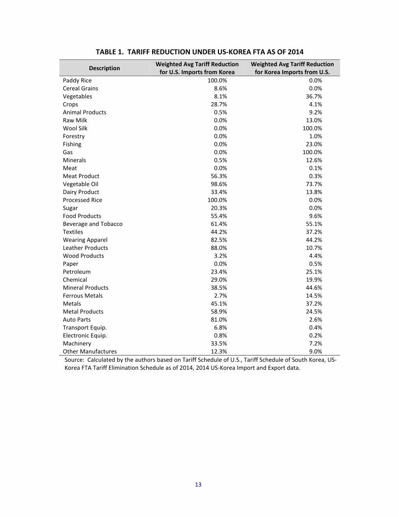
both countries for each relevant GTAP sector. The results are presented in Table 1.

Note that Table 1 only lists the first 42 GTAP sectors. GTAP Sectors 43 to 57 are service sectors,

which are not typically involved in international trade. The weighted average tariff reductions

of all sectors range from 0% to 100%. There are three possible reasons that a GTAP sector has a

zero weighted average tariff reduction as of 2014. First, the commodities were duty free

before the FTA, and remained so after the FTA. Second, as of 2014, the tariff reduction process

has not kicked in for the commodities under the GTAP sector. Third, in the cases that no

commodities were imported or exported for a GTAP sector in 2014, we assume the tariff level

remains same.

Our simulations were implemented by changing the power of the tax on imports of affected

tradable commodities from source country to destination country according to the tariff

reduction information presented in Table 1. The simulations were implemented in three

groups: a) adjusting the tariff on import side only (goods imported from Korea to the U.S.); 2)

adjusting the tariff from the export side only (in other words, goods imported from the U.S. to

Korea); and 3) shocking tariff on both the import and export side simultaneously. The default

closure rules of the GTAP Model were adopted for all the simulations. Specifically, the factor

endowments (e.g., the total supply of labor, capital and land) are fixed, whereas factor prices

are adjusted to restore full employment. In addition, the saving rate is assumed to be

exogenous and constant; hence, the quantity of savings changes as income changes.

13

TABLE 1. TARIFF REDUCTION UNDER US-KOREA FTA AS OF 2014

Description Weighted Avg Tariff Reduction for U.S. Imports from Korea

Weighted Avg Tariff Reduction for Korea Imports from U.S.

Paddy Rice 100.0% 0.0% Cereal Grains 8.6% 0.0% Vegetables 8.1% 36.7% Crops 28.7% 4.1% Animal Products 0.5% 9.2% Raw Milk 0.0% 13.0% Wool Silk 0.0% 100.0% Forestry 0.0% 1.0% Fishing 0.0% 23.0% Gas 0.0% 100.0% Minerals 0.5% 12.6% Meat 0.0% 0.1% Meat Product 56.3% 0.3% Vegetable Oil 98.6% 73.7% Dairy Product 33.4% 13.8% Processed Rice 100.0% 0.0% Sugar 20.3% 0.0% Food Products 55.4% 9.6% Beverage and Tobacco 61.4% 55.1% Textiles 44.2% 37.2% Wearing Apparel 82.5% 44.2% Leather Products 88.0% 10.7% Wood Products 3.2% 4.4% Paper 0.0% 0.5% Petroleum 23.4% 25.1% Chemical 29.0% 19.9% Mineral Products 38.5% 44.6% Ferrous Metals 2.7% 14.5% Metals 45.1% 37.2% Metal Products 58.9% 24.5% Auto Parts 81.0% 2.6% Transport Equip. 6.8% 0.4% Electronic Equip. 0.8% 0.2% Machinery 33.5% 7.2% Other Manufactures 12.3% 9.0% Source: Calculated by the authors based on Tariff Schedule of U.S., Tariff Schedule of South Korea, US-Korea FTA Tariff Elimination Schedule as of 2014, 2014 US-Korea Import and Export data.

14

V. AGGREGATE AND SECTORAL IMPACTS OF US-KOREA FTA

A. Aggregate Impacts

There are several metrics that are often used to evaluate policies and practices. Two widely-

cited macroeconomic indicators are Gross Domestic Product (GDP) and employment. However,

when federal government agencies evaluate the economic impacts of change in their policies or

programs, they are directed by the Office of Management and Budget (OMB) to use different

measures, referred to as “economic welfare,” that better capture changes in the economic

well-being of the U.S. public. These measures are also used by agencies such as the U.S.

International Trade Commission (ITC) to evaluate the impacts of trade policies. On the other

hand, businesses and financial analysts are more likely to focus on individual firm or industry

profits or sales revenue, the latter being equivalent to gross output.

The economic benefits of tariff reduction under the US-Korea FTA were evaluated in three

scenarios. The first evaluates the impacts from reductions of the U.S. import tariffs on

commodities from Korea as shown in the second column of Table 1. The second scenario

evaluates the impacts from reductions of Korea’s tariffs on the commodities imported from the

U.S as shown in the last column of Table 1. The third scenario measures the aggregate impacts

of the FTA involving reductions of import tariffs in both countries.

Many factors affect the overall impacts of tariff reductions under an FTA, which include relative

price changes of import and export, domestic demand and supply elasticities, trade elasticities,

and changes in relative competitiveness of domestic industries. Changes in import tariffs have

direct effects on sectors in which the tariffs are changed and indirect effects (to be discussed

15

further below) on other sectors and the economy as a whole. Our simulation results indicate

that whenever there is a tariff reduction on Korean imports into the U.S. or U.S. imports into

Korea, the imports or exports of the relevant U.S. sectors will increase, respectively, while the

imports and exports of nearly all other sectors decrease. This decrease is attributable to the

substitution effect stemming from the tariff reductions exceeding the output effect. Sectoral

variations depend on the key factors mentioned earlier, especially the import and export

elasticities, given that we are focusing on trade.

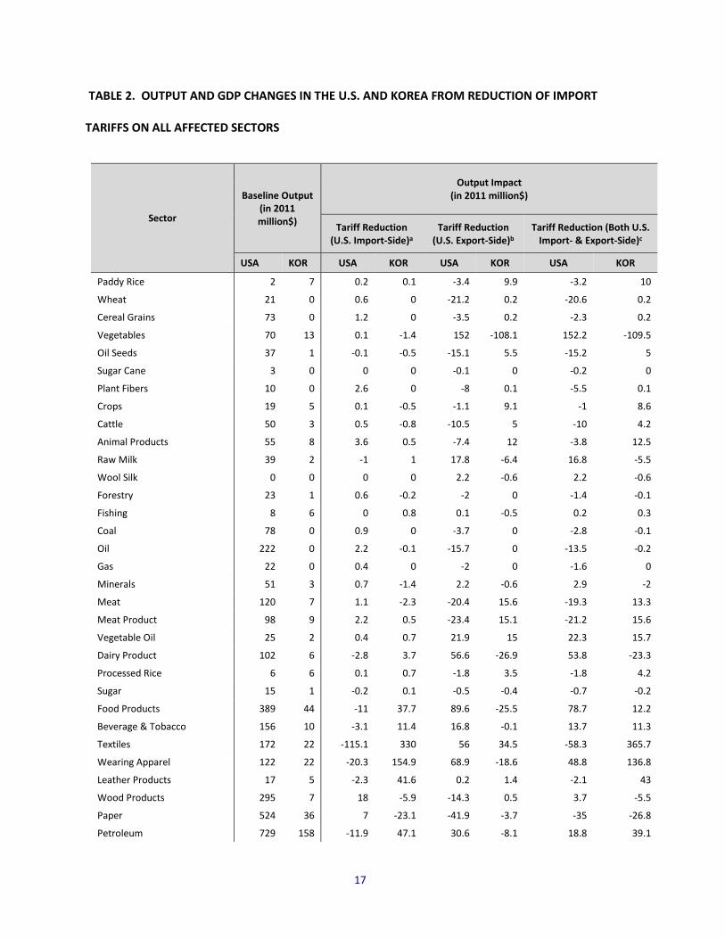
Table 2 presents the impacts on Gross Output (in real terms) of all sectors for both the U.S. and

Korea for the reduction of import tariffs as a result of the implementation of the FTA between

the two countries. The total GDP impacts are presented in the last row of the table. Total GDP

increases for the U.S. and Korea are $45 million and $162.3 million, respectively. However, the

results indicate a potential Gross Output loss of $142.7 million for the U.S., but a $322.3 million

gain for Korea.

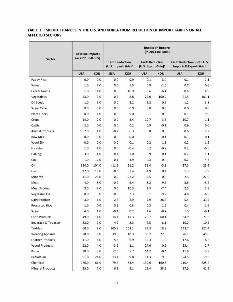
Table 3 presents the sectoral impacts for both the U.S. and Korea in relation to direct changes

in imports. The results indicate that the reduction of import tariff increases the total imports in

the U.S. and Korea, with level changes of $1.56 billion and $1.2 billion, respectively, in 2014.

Although changes in total imports on net from the reduction of tariffs of all the directly affected

sectors are positive, imports by some sectors decline as a result of the dominating output effect

over the substitution effect.

Table 4 presents the total Economic Welfare (EW) impacts of tariff reductions in terms of

Equivalent Variation, which represents an approximation of consumer surplus changes. In the

16

GTAP model, economic welfare is expressed in terms of changes in consumption and savings

(approximately equal to disposable personal income) in billions of 2011 dollars. The

implementation of the FTA between the U.S. and Korea is projected to result in a positive

impact in terms of EW changes on the order of well over $300 million for each country.

B. Decomposition Analysis of Welfare Impacts

The results can be further explained by a decomposition of the overall EW effect into various

components. The GTAP model offers an option of separating six causal factors, though for our

analysis three of them would change imperceptibly and thus are held constant. Of the

remaining three factors, which are presented in Table 4, the first is the Allocation Effect, which

pertains to the price distorting effects of the duties. The second causal factor is the standard

Commodity Terms of Trade Effect. The third is an Investment-Savings Terms of Trade Effect.

Table 4 presents not only the decomposed welfare effects for the U.S. and Korea, but also the

spillover effects on Rest of the World. On both the import and the export sides, the Allocation

Effect is positive for both the U.S. and Korea, since tariff reduction represents the correction of

price distortions caused by import taxes. However, the impacts are negative for Rest of the

World as a whole because the FTA increases trade between the two signatories and reduced

their trade with Rest of the World. The negative impacts to Rest of the World slightly more

than offset the positive impacts for the U.S. and Korea on the import side, but are lower than

the positive impacts to the two countries on the export side.

17

TABLE 2. OUTPUT AND GDP CHANGES IN THE U.S. AND KOREA FROM REDUCTION OF IMPORT

TARIFFS ON ALL AFFECTED SECTORS

Sector

Baseline Output (in 2011 million$)

Output Impact (in 2011 million$)

Tariff Reduction (U.S. Import-Side)a

Tariff Reduction (U.S. Export-Side)b

Tariff Reduction (Both U.S. Import- & Export-Side)c

USA KOR USA KOR USA KOR USA KOR

Paddy Rice 2 7 0.2 0.1 -3.4 9.9 -3.2 10

Wheat 21 0 0.6 0 -21.2 0.2 -20.6 0.2

Cereal Grains 73 0 1.2 0 -3.5 0.2 -2.3 0.2

Vegetables 70 13 0.1 -1.4 152 -108.1 152.2 -109.5

Oil Seeds 37 1 -0.1 -0.5 -15.1 5.5 -15.2 5

Sugar Cane 3 0 0 0 -0.1 0 -0.2 0

Plant Fibers 10 0 2.6 0 -8 0.1 -5.5 0.1

Crops 19 5 0.1 -0.5 -1.1 9.1 -1 8.6

Cattle 50 3 0.5 -0.8 -10.5 5 -10 4.2

Animal Products 55 8 3.6 0.5 -7.4 12 -3.8 12.5

Raw Milk 39 2 -1 1 17.8 -6.4 16.8 -5.5

Wool Silk 0 0 0 0 2.2 -0.6 2.2 -0.6

Forestry 23 1 0.6 -0.2 -2 0 -1.4 -0.1

Fishing 8 6 0 0.8 0.1 -0.5 0.2 0.3

Coal 78 0 0.9 0 -3.7 0 -2.8 -0.1

Oil 222 0 2.2 -0.1 -15.7 0 -13.5 -0.2

Gas 22 0 0.4 0 -2 0 -1.6 0

Minerals 51 3 0.7 -1.4 2.2 -0.6 2.9 -2

Meat 120 7 1.1 -2.3 -20.4 15.6 -19.3 13.3

Meat Product 98 9 2.2 0.5 -23.4 15.1 -21.2 15.6

Vegetable Oil 25 2 0.4 0.7 21.9 15 22.3 15.7

Dairy Product 102 6 -2.8 3.7 56.6 -26.9 53.8 -23.3

Processed Rice 6 6 0.1 0.7 -1.8 3.5 -1.8 4.2

Sugar 15 1 -0.2 0.1 -0.5 -0.4 -0.7 -0.2

Food Products 389 44 -11 37.7 89.6 -25.5 78.7 12.2

Beverage & Tobacco 156 10 -3.1 11.4 16.8 -0.1 13.7 11.3

Textiles 172 22 -115.1 330 56 34.5 -58.3 365.7

Wearing Apparel 122 22 -20.3 154.9 68.9 -18.6 48.8 136.8

Leather Products 17 5 -2.3 41.6 0.2 1.4 -2.1 43

Wood Products 295 7 18 -5.9 -14.3 0.5 3.7 -5.5

Paper 524 36 7 -23.1 -41.9 -3.7 -35 -26.8

Petroleum 729 158 -11.9 47.1 30.6 -8.1 18.8 39.1

18

Chemical 1086 215 -23.4 126.4 168.6 22.1 145.4 148.7

Mineral Products 162 33 0 -16.1 88.5 -23.8 88.5 -39.9

Ferrous Metals 213 166 9.2 -192.8 -57.9 -4.9 -48.8 -197.8

Metals 180 44 7.4 -20.4 39 0.5 46.1 -19.9

Metal Products 392 77 -37.7 52.8 14.3 -26.3 -23.4 26.5

Auto Parts 618 142 -111.1 603.5 -119.4 33.8 -230.6 637.6

Transport Equip. 277 60 79.7 -235.4 -145.4 33.8 -65.9 -201.8

Electronic Equip. 563 217 118.7 -613.8 -294 176.3 -175.8 -438.5

Machinery 1158 191 67.6 -305.1 -267.6 3.4 -200.6 -302.1

Other Manufactures 119 43 8.1 16.5 -5.7 -12.4 2.4 4.1

Electricity 421 48 -2.8 17.2 6.5 1.6 3.7 18.8

Gas 74 0 -0.4 0.2 -0.2 0 -0.7 0.1

Water 143 7 -1.1 3.7 1.5 -0.1 0.4 3.6

Construction 1798 179 85.5 65 200.9 95.8 286.8 160.8

Trade 3187 254 3 37.9 16 29.4 19 67.3

Transport Nec 692 88 7.3 -23.4 -10.4 -1.5 -3.1 -24.9

Sea Transport 84 30 1 -10.2 -2.3 -0.1 -1.3 -10.3

Air Transport 266 21 7.7 -9.6 -21.9 0.2 -14.3 -9.4

Communication 588 54 -2.2 0.4 -8.3 -1.2 -10.4 -0.8

Financial Service 1745 83 2.9 -8.4 -35.4 -7 -32.5 -15.5

Insurance 609 37 -4.8 2.9 -22.1 -3.5 -26.9 -0.6

Business Service 2333 169 26.8 -54.2 -91.8 6.8 -65.3 -47.4

Recreation 1360 54 -11.3 2.2 11.3 -2.9 0 -0.7

Public Service 5115 293 -69.5 58.8 48 -21.8 -21.5 37

Dwellings 1536 78 -23.1 20.6 14.4 -17.5 -8.8 3.1

Total Output Impact 28275 2970 11.8 113 -154.4 208.5 -142.7 322.3

Total GDP Impact 15534 1202 11 92.3 35 70.3 45 162.3 a. The scenario includes the shocks of reductions of US import tariffs for commodities from Korea in the selected sectors (see Table 1). The figures in the table represent the macroeconomic impacts on all sectors of tariff reduction in the above selected sectors. b. The scenario includes the shocks of reductions of Korea import tariffs for commodities from the U.S. in the selected sectors (see Table 1). The figures in the table represent the macroeconomic impacts on all sectors of tariff reduction in the above selected sectors. c. The scenario includes reductions of import tariffs in both the U.S. and Korea.

19

TABLE 3. IMPORT CHANGES IN THE U.S. AND KOREA FROM REDUCTION OF IMPORT TARIFFS ON ALL AFFECTED SECTORS

Sector Baseline Imports (in 2011 million$)

Impact on Imports (in 2011 million$)

Tariff Reduction (U.S. Import-Side)a

Tariff Reduction (U.S. Export-Side)b

Tariff Reduction (Both U.S. Import- & Export-Side)c

USA KOR USA KOR USA KOR USA KOR

Paddy Rice 0.0 0.0 0.0 0.9 0.1 -8.0 0.1 -7.1

Wheat 1.0 2.0 0.0 1.5 0.8 -1.0 0.7 0.6

Cereal Grains 1.0 14.0 0.0 10.9 0.6 -6.1 0.6 4.9

Vegetables 23.0 3.0 -0.6 2.8 22.0 100.2 21.5 103.1

Oil Seeds 1.0 6.0 0.0 3.2 1.2 0.6 1.2 3.8

Sugar Cane 0.0 0.0 0.0 0.0 0.0 0.0 0.0 0.0

Plant Fibers 0.0 1.0 0.0 9.0 0.1 0.8 0.1 9.9

Crops 14.0 2.0 0.0 2.4 10.7 -3.5 10.7 -1.1

Cattle 2.0 0.0 0.0 0.2 0.9 -0.1 0.9 0.0

Animal Products 2.0 1.0 -0.2 6.3 0.8 0.8 0.6 7.2

Raw Milk 0.0 0.0 0.0 0.0 0.1 -0.1 0.1 -0.1

Wool Silk 0.0 0.0 0.0 0.1 0.2 1.1 0.2 1.2

Forestry 1.0 1.0 0.0 -0.4 0.2 -0.2 0.2 -0.5

Fishing 3.0 1.0 -0.1 1.0 0.9 0.1 0.7 1.1

Coal 1.0 17.0 -0.1 4.9 0.3 -0.4 0.2 4.6

Oil 324.0 104.0 -11.1 31.2 38.4 -5.3 27.3 25.9

Gas 17.0 16.0 -0.6 7.4 1.9 0.4 1.3 7.9

Minerals 11.0 28.0 0.0 -22.2 2.5 -0.6 2.5 -22.9

Meat 4.0 3.0 -0.2 6.4 3.8 -9.5 3.6 -3.2

Meat Product 3.0 2.0 0.0 10.3 2.5 -7.4 2.5 2.8

Vegetable Oil 8.0 3.0 -0.3 2.3 5.1 -9.2 4.8 -6.9

Dairy Product 3.0 1.0 2.5 2.9 2.9 28.3 5.4 31.2

Processed Rice 1.0 0.0 0.1 0.3 0.3 -2.2 0.4 -1.9

Sugar 4.0 1.0 -0.1 0.2 1.6 -0.2 1.5 -0.1

Food Products 49.0 11.0 14.1 11.3 20.7 60.1 34.9 71.5

Beverage & Tobacco 22.0 2.0 4.6 2.3 5.5 8.1 10.2 10.5

Textiles 60.0 8.0 105.9 102.1 37.3 18.9 143.7 121.4

Wearing Apparel 78.0 6.0 39.8 18.3 36.2 27.3 76.1 45.6

Leather Products 41.0 4.0 5.3 6.9 12.3 1.2 17.6 8.2

Wood Products 52.0 4.0 -3.6 2.1 27.0 0.6 23.4 2.7

Paper 30.0 5.0 -2.6 5.7 14.2 -0.4 11.6 5.3

Petroleum 91.0 21.0 13.1 9.8 11.3 9.5 24.5 19.3

Chemical 276.0 61.0 79.4 64.4 130.6 160.5 210.4 225.2

Mineral Products 23.0 7.0 6.1 3.1 11.4 38.9 17.5 41.9

20

Ferrous Metals 41.0 27.0 -4.3 -1.3 11.6 7.0 7.3 5.7

Metals 66.0 21.0 10.3 -2.5 24.7 30.7 35.0 28.2

Metal Products 46.0 8.0 51.9 13.5 25.6 46.4 77.6 60.0

Auto Parts 225.0 13.0 199.1 51.5 81.6 7.6 280.8 59.1

Transport Equip. 53.0 9.0 0.6 10.3 21.1 3.0 21.7 13.4

Electronic Equip. 289.0 54.0 -17.6 1.7 89.0 10.6 71.6 12.2

Machinery 367.0 76.0 85.6 72.5 198.7 100.1 284.5 172.6

Other Manufactures 85.0 4.0 -2.9 8.0 35.3 20.2 32.4 28.3

Electricity 4.0 0.0 -0.2 0.0 1.9 0.0 1.7 0.0

Gas 1.0 0.0 0.0 0.2 0.4 0.0 0.4 0.2

Water 0.0 0.0 0.0 0.3 0.2 0.0 0.2 0.3

Construction 4.0 3.0 -0.5 2.6 1.8 -0.1 1.3 2.5

Trade 27.0 15.0 -1.6 25.0 10.9 -3.1 9.3 21.9

Transport Nec 51.0 12.0 -2.1 14.8 12.5 0.7 10.4 15.4

Sea Transport 3.0 7.0 -0.1 -2.4 0.6 0.0 0.6 -2.4

Air Transport 42.0 9.0 -1.9 2.7 6.8 0.2 5.0 3.0

Communication 13.0 2.0 -0.7 2.5 4.6 0.2 3.9 2.6

Financial Service 41.0 3.0 -3.5 4.8 15.7 0.5 12.3 5.3

Insurance 41.0 2.0 -1.4 1.7 14.4 0.0 13.0 1.7

Business Service 101.0 21.0 -7.2 30.6 34.5 7.7 27.3 38.3

Recreation 15.0 6.0 -0.8 8.8 5.1 -0.2 4.3 8.6

Public Service 47.0 7.0 -2.0 9.8 8.3 2.2 6.3 12.0

Dwellings 0.0 0.0 0.0 0.0 0.0 0.0 0.0 0.0

Total Impact on Imports 2,706.0 633.0 552.2 562.6 1,009.3 636.8 1,563.9 1,200.9 a. The scenario includes the shocks of reductions of US import tariffs for commodities from Korea in the selected sectors (see Table 1). The figures in the table represent the macroeconomic impacts on all sectors of tariff reduction in the above selected sectors. b. The scenario includes the shocks of reductions of Korea import tariffs for commodities from the U.S. in the selected sectors (see Table 1). The figures in the table represent the macroeconomic impacts on all sectors of tariff reduction in the above selected sectors. c. The scenario includes reductions of import tariffs in both the U.S. and Korea.

21

TABLE 4. WELFARE DECOMPOSITION OF REDUCTIONS OF IMPORT TARIFFS ON ALL AFFECTED SECTORS IN FY 2014 DUE TO US-KOREA FTA

(million 2011 dollars)

Welfare Decomposition

IMPa EXPb BOTHc USA KOR ROW USA KOR ROW USA KOR ROW

Allocation Effect 10.8 92.2 -142.1 34.7 70.2 -46.7 45.3 162.3 -189.1 Commodity Terms of Trade -78.3 317.0 -238.9 330.2 -70.1 -260.1 252.6 247.0 -499.7 Invest.-Savings Terms of Trade -42.2 -12.2 54.4 112.2 -2.3 -109.9 70.1 -14.4 -55.7 Total -109.6 397.1 -326.6 477.1 -2.2 -416.7 368.1 394.9 -744.5 a. This set of columns summarizes the impacts of reductions of US import tariffs for commodities from Korea in the selected sectors (see Table 1). The figures in the table represent the macroeconomic impacts on all sectors of tariff reduction in the above selected sectors. b. This set of columns summarizes the impacts of reductions of Korea import tariffs for commodities from the U.S. in the selected sectors (see Table 1). The figures in the table represent the macroeconomic impacts on all sectors of tariff reduction in the above selected sectors. c. This set of columns summarizes the impacts of reductions of import tariffs in both the U.S. and Korea.

The two Terms of Trade effects are negative for the U.S. from an import tariff reduction, but are

positive if the reduction of the tariff is on U.S. exports to Korea. Since the positive Terms of

Trade effects on the export side for U.S. exports to Korea exceed the negative effects on the

import side from Korea to the U.S., the combined Terms of Trade impacts for the U.S.,

presented in the third to last column of Table 3, are positive ($253 million and $70 million,

respectively). Similar to the Allocation Effect, the Terms of Trade Effect is found to be negative

for the Rest of the World in all three scenarios.

The overall EW gains from tariff reductions of all related products implemented under the US-

Korea FTA are estimated to be $368 million for the U.S. and $395 million for Korea. Conversely,

the Rest of the World would experience an EW loss of $745 million due to the implementation

of the US-Korea FTA. The overall negative impacts on the Rest of the World result from the

displacement and diversion of trade flows between the two US-Korea FTA partner countries

22

and all the other countries as an aggregate. However, we note that this study is a comparative

static analysis that only focuses on the impacts of the US-Korea FTA. Trading agreements either

between the U.S. or Korea and other countries (such as the on-going negotiation of the China-

Japan-South Korea FTA) might mute or enhance the impacts of the US-Korea FTA on the U.S. or

Korean economy. However, the net impacts of multiple bilateral trade agreements that involve

the U.S. or Korea are beyond the scope of this study.

C. Sensitivity Analysis

In order to validate our findings of the welfare impacts of the US-Korea FTA, we also performed

sensitivity analysis to evaluate how the modeling results vary in response to the changes in the

value of key parameters of the GTAP model. The sensitivity analysis was conducted based on

the aforementioned three scenarios with respect to variations in two key parameters in the

GTAP model: Armington elasticities of substitution between domestic and imported

commodities (ESUBD) and elasticities of substitution between primary factors in production

(ESUBVA). The base case simulation was based on the original parameters provided by the

GTAP data base (see Appendix A), whereas the sensitivity analysis examines the variations of

the welfare impacts with the same level of shocks for each scenario, but varied by adjusting the

parameters for each sector down and up by 50%, independently and respectively. For instance,

the value of ESUBD for wool manufacturing varied in the range from 2.025 (a 50% decrease) to

6.075 (a 50% increase). The sensitivity analysis for each policy simulation scenario for the

ESUBD and ESUBVA was executed 114 times and 116 times, respectively. Hence, 690

23

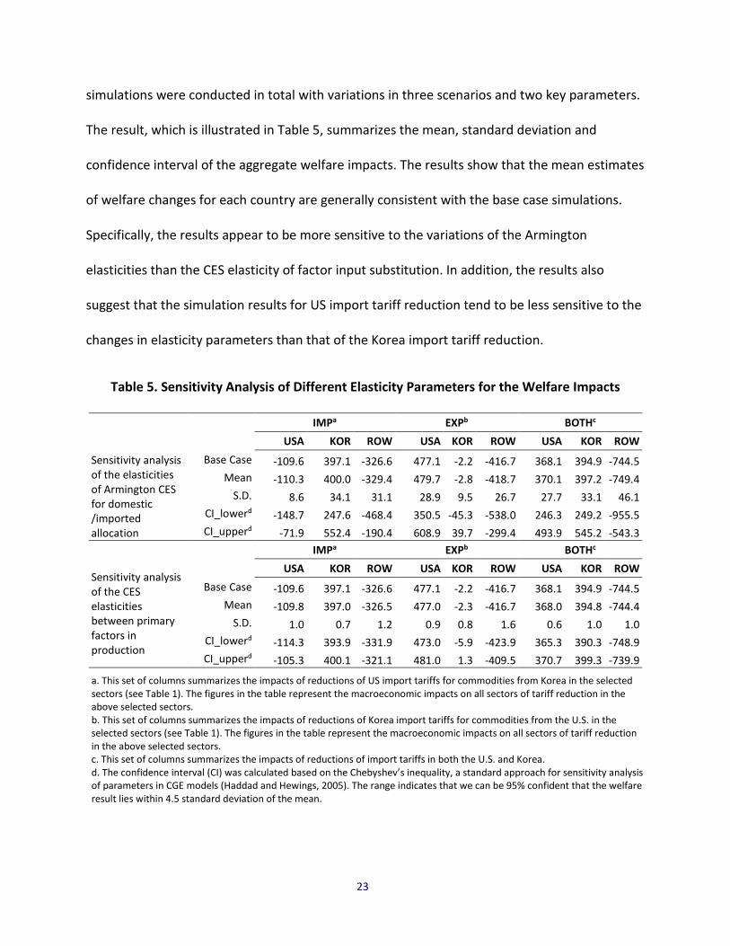
simulations were conducted in total with variations in three scenarios and two key parameters.

The result, which is illustrated in Table 5, summarizes the mean, standard deviation and

confidence interval of the aggregate welfare impacts. The results show that the mean estimates

of welfare changes for each country are generally consistent with the base case simulations.

Specifically, the results appear to be more sensitive to the variations of the Armington

elasticities than the CES elasticity of factor input substitution. In addition, the results also

suggest that the simulation results for US import tariff reduction tend to be less sensitive to the

changes in elasticity parameters than that of the Korea import tariff reduction.

Table 5. Sensitivity Analysis of Different Elasticity Parameters for the Welfare Impacts

Sensitivity analysis of the elasticities of Armington CES for domestic /imported allocation

IMPa EXPb BOTHc USA KOR ROW USA KOR ROW USA KOR ROW

Base Case -109.6 397.1 -326.6 477.1 -2.2 -416.7 368.1 394.9 -744.5 Mean -110.3 400.0 -329.4 479.7 -2.8 -418.7 370.1 397.2 -749.4

S.D. 8.6 34.1 31.1 28.9 9.5 26.7 27.7 33.1 46.1 CI_lowerd -148.7 247.6 -468.4 350.5 -45.3 -538.0 246.3 249.2 -955.5 CI_upperd -71.9 552.4 -190.4 608.9 39.7 -299.4 493.9 545.2 -543.3

IMPa EXPb BOTHc

Sensitivity analysis of the CES elasticities between primary factors in production

USA KOR ROW USA KOR ROW USA KOR ROW Base Case -109.6 397.1 -326.6 477.1 -2.2 -416.7 368.1 394.9 -744.5

Mean -109.8 397.0 -326.5 477.0 -2.3 -416.7 368.0 394.8 -744.4 S.D. 1.0 0.7 1.2 0.9 0.8 1.6 0.6 1.0 1.0

CI_lowerd -114.3 393.9 -331.9 473.0 -5.9 -423.9 365.3 390.3 -748.9 CI_upperd -105.3 400.1 -321.1 481.0 1.3 -409.5 370.7 399.3 -739.9

a. This set of columns summarizes the impacts of reductions of US import tariffs for commodities from Korea in the selected sectors (see Table 1). The figures in the table represent the macroeconomic impacts on all sectors of tariff reduction in the above selected sectors. b. This set of columns summarizes the impacts of reductions of Korea import tariffs for commodities from the U.S. in the selected sectors (see Table 1). The figures in the table represent the macroeconomic impacts on all sectors of tariff reduction in the above selected sectors. c. This set of columns summarizes the impacts of reductions of import tariffs in both the U.S. and Korea. d. The confidence interval (CI) was calculated based on the Chebyshev’s inequality, a standard approach for sensitivity analysis of parameters in CGE models (Haddad and Hewings, 2005). The range indicates that we can be 95% confident that the welfare result lies within 4.5 standard deviation of the mean.

24

D. Sectoral Impacts

Our analysis indicates that the US-Korea FTA generates a divergence of outcomes, especially for

the U.S. From the standpoint of the U.S., welfare gains are estimated to be $368 million, GDP

gains are estimated to be $45 million, and total gross output (sales revenue) is estimated to

incur a net loss of $143 million. Moreover, 34 out of 57 sectors of the US economy are

estimated to incur gross output losses. This includes three advanced manufacturing sectors

estimated to incur gross output reductions in excess of $175 million each. Ironically, the

sectors that are estimated to gain the most are primary sectors in agricultural and mining,

construction, and primary manufacturing. These results indicate the continued shift in

comparative advantage away from US manufacturing with respect to rising economies such as

that of South Korea.

The sectors incurring the greatest gross output losses, in descending order, are Auto Parts,

Machinery, and Electronic Equipment, all with decreases in excess of $175 million. Other

sectors with losses in excess of $50 million are Business Services and Textiles. On the other

hand, the biggest winners, in descending order, are Construction, Vegetable Crops, Chemicals,

Mineral Products, Food Processing, and Dairy Products, all with gains in excess of $50 million.

There is symmetry in these results between the U.S. and Korea, in that in nearly all cases the

gains or losses are reversed for the two countries.4 The biggest gains for Korean sectors are

4 There are a couple of notable exceptions to this statement, such as the case of Transportation Equipment, of Electronic Equipment, and of Machinery, where the gross output declines in both countries. However, this can be explained for the first two sectors by the fact that there is hardly any tariff reduction for these goods at all in either country (see Table 1). Therefore, resources will shift away from them and move to other sectors that benefit from high tariff reductions. In case of the Machinery sector there is a significant tariff decrease applicable to imports from Korea to the US. However, it is still modest compared to many other sectors.

25

estimated to be in Auto Parts and Textiles, with gross output increases of $638 million and $366

million, respectively. Of course, in relative terms, the changes in gross output in U.S. industries

is relatively small, with only four sectors experiencing changes in excess of one-tenth of one

percent. On the South Korean side, however, the majority of sectors experience changes in

gross output in excess of this threshold.

With reductions in tariffs, inter-country trade expands. On the U.S. side, all sectors will

experience an increase in imports. Sectors that are expected to have the biggest increases in

imports, in descending order, are Machinery, Auto Parts, Chemicals, and Textiles, all with

increases in excess of $140 million. On the South Korean side, the sectors that are expected to

have the biggest increase in import are similar as those in the U.S. The sectors with an import

increase in excess of $100 million are, in descending order, Chemicals, Machinery, Textiles, and

Vegetables. A few sectors are expected to have a decline in imports. However, except for

Minerals (with a reduction of $23 million), all other sectors will only experience a decrease of

less than $7 million. Similarly, the import changes in the U.S. are relatively small in percentage

terms, with only four sectors exceeding a one-tenth of one percent increase. For South Korea,

however, the majority of sectors experience changes in imports in excess of this threshold, with

six sectors experiencing a change of more than one percent.

Thus, the results indicate various trade-offs. First, while both countries are estimated to receive

welfare gains, the South Korean gains are slightly higher in absolute terms and more than 12

times higher in relative terms, which is proxied by personal income changes. In a possible new

era of “America first”, this relative imbalance may be viewed by the new Presidential

26

administration as being problematic. The divergence becomes even more extreme from a U.S.

perspective if one considers GDP gains being more than 3.5 times higher for Korea in absolute

terms and nearly 50 times higher in relative terms. In terms of gross output impacts, the

outcome may be even more problematic from a U.S. standpoint, because the impacts on this

indicator are overall negative. This means that total industry revenues, and likely profits as well,

will fall, with 36 of 57 sectors expected to experience losses, including several major

manufacturing industries located primarily in geographic areas of the country that have been

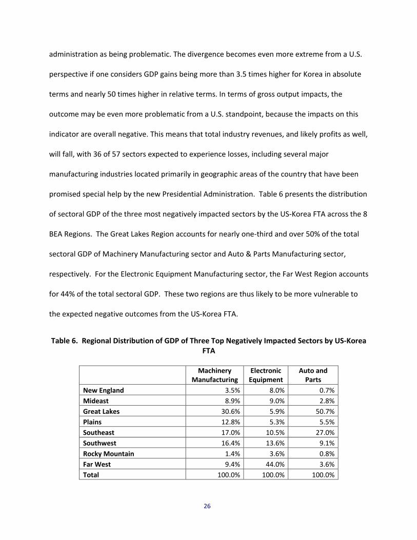
promised special help by the new Presidential Administration. Table 6 presents the distribution

of sectoral GDP of the three most negatively impacted sectors by the US-Korea FTA across the 8

BEA Regions. The Great Lakes Region accounts for nearly one-third and over 50% of the total

sectoral GDP of Machinery Manufacturing sector and Auto & Parts Manufacturing sector,

respectively. For the Electronic Equipment Manufacturing sector, the Far West Region accounts

for 44% of the total sectoral GDP. These two regions are thus likely to be more vulnerable to

the expected negative outcomes from the US-Korea FTA.

Table 6. Regional Distribution of GDP of Three Top Negatively Impacted Sectors by US-Korea FTA

Machinery

Manufacturing Electronic Equipment

Auto and Parts

New England 3.5% 8.0% 0.7% Mideast 8.9% 9.0% 2.8% Great Lakes 30.6% 5.9% 50.7% Plains 12.8% 5.3% 5.5% Southeast 17.0% 10.5% 27.0% Southwest 16.4% 13.6% 9.1% Rocky Mountain 1.4% 3.6% 0.8% Far West 9.4% 44.0% 3.6% Total 100.0% 100.0% 100.0%

27

In Appendix C, we further examined the percentage changes in sectoral real GDP of the three

sectors that are predicted to be most negatively affected by the US-Korea FTA over the period

of 2012 to 2015.

E. Comparison to Other Studies

We now compare our results with those of other analysts of the US-Korea FTA. First, we point

out that this comparison is made difficult by the fact that all previous studies were performed

before 2008, did not necessarily reflect the current FTA provisions, and simulated a full

reduction of tariffs. We refer the reader back to Table 1 to note that our evaluation pertains to

the impacts of the FTA as in force in 2014, a time at which the average tariff elimination ratio

was about 50%. On the other hand, the comparison is facilitated by the fact that all of the

previous studies used a CGE model, and all but one used an earlier (but thus more sectorally

aggregated) version of the GTAP Model.

Cheong and Wang (1999) estimated welfare gains of up to $4.8 billion for Korea and $3.7 billion

for the U.S. annually for a 100% tariff reduction in all sectors. McDaniel and Fox (2001)

estimated welfare gains of $19.6 billion for the U.S. and $3.9 billion annually for Korea from a

100% elimination of the bilateral trade barriers. Choi and Schott (2001) estimated that the net

welfare gains would be evenly allocated across both Korea and the U.S., in the range of $1.5

billion to $8.9 billion for the U.S. and $1.7 billion to $10.9 billion for Korea. Schott et al. (2006)

estimated the welfare gains of a full FTA as $20.2 billion for Korea and $0.8 billion for the U.S.

Kiyota and Stern (2007) used a multiregional CGE model with 27 economic sectors, known as

the “Michigan Model”. They estimated that the FTA would increase Korea’s welfare by $9.3

28

billion, with $4.48 billion coming from the bilateral removal of manufacturing sector barriers

and $5.46 billion from bilateral removal of services sector barriers. U.S. economic welfare was

estimated to increase by $25.1 billion, with $7.3 billion coming from elimination of

manufacturing sector tariffs and $19.2 billion from elimination of services sector barriers.

At the sectoral level, McDaniel and Fox (2001) estimated that Agriculture would incur the

biggest output increase, while Textiles and Apparel would incur the biggest decline in the U.S.

Korea was estimated to experience the reverse of these sectoral impacts. Schott et al. (2006)

generated similar sectoral findings. Our results are similar in finding the major sectoral

expansion for the U.S. being in various types of Agricultural commodity sectors, and the Textile

sector experiencing relatively large losses. However, we also estimated large losses in various

Machinery and Equipment sectors. This might be explained by the ascendance of the Korean

auto industry and by rapid technological innovations in Korean cell phones that have made

them much more competitive than 10 to 15 years prior.

Again, overall, the previous estimates of aggregate welfare gains are typically much higher than

ours for both countries, though our results are similar to the range found in studies by Choi and

Schott (2001) and Schott et al. (2016). Thus, we can consider our aggregate estimates to be on

the conservative side. At the sectoral level, there is a strong similarity between ours and

previous studies, and the differences can readily be explained by the change in conditions

between their year of analysis and ours.

29

VII. CONCLUSIONS

Free Trade Agreements aim to eliminate trade barriers between partner countries, increase

trade flows of goods and services between them, and improve overall economic efficiency. An

increasing number of FTAs and preferential trade programs have been established between the

U.S. and other countries and regions.

In this study, we evaluated the economic impacts of the U.S.-Korea FTA. We adapted a state of

the art methodology and applied the latest version of GTAP Model in the economic impact

analysis, with a focus on the impacts of the tariff reduction/elimination provisions in the FTA.

The results indicate that the bilateral tariff reductions of import commodities under the FTA

result in an increase in U.S. welfare (approximately equivalent to personal income) by about

$368.1 million, reflecting a combination of substitution and output effects, as well as the net

effects in relation to the terms of trade. Among the two effects, the Terms of Trade effect

accounts for over 87% of the total welfare increase stemming from the reduction of import

tariffs between the two countries.

However, the current policy climate in the U.S. is likely to renew attention to other metrics.

Therefore, we have measured the impacts of the U.S.-Korea FTA on GDP, which is of interest to

many decision makers, and estimated expected total impacts on this indicator for the U.S.

economy to be only $45 million. On the other hand, since industry executives and stock market

analysts are likely to be more interested in measures of business performance, such as sales

revenue and profits, we measured sectoral Gross Output impacts and found mixed results, with

30

the largest increases expected to be in U.S. sectors that had their tariffs reduced the most by

Korea.

Overall, the results are ambiguous, suggesting several trade-offs. Positive welfare gains

between the U.S. and South Korea are about the same in absolute terms, but favor the latter in

relative terms, and very heavily so in terms of GDP gains. Moreover, the U.S. is projected to

incur an overall total loss of Gross Output (sales revenue), with 34 of 57 sectors experiencing

losses, including several major manufacturing sectors that are heavily concentrated in

geographic areas that have been promised “job return” by the new Presidential Administration.

The fact that so many U.S. sectors are estimated to suffer decreases in Gross Output, and hence

employment, is also likely to be problematic from a political standpoint in terms of potential

widespread opposition by so many sectors estimated to lose jobs.

We note the tariff elimination process involves different tariff reduction phase-in stages for

different types of commodities over the course of the future decade or so. Therefore, a

dynamic CGE model might be needed to fully capture time-related features of the trade

liberalization process. In addition, this paper only focuses on the modeling of removals of

merchandise trade barriers. Since other aspects of trade liberalization, such as service trade

and foreign investment liberalization, are not covered in the analysis, the economic impacts of

the U.S. entering into trade reforms with foreign trading partners presented here can be

viewed as a conservative estimate of the potential impacts of an FTA.

31

REFERENCES

Abe, K. 2007. “Assessing the Economic Impacts of Free Trade Agreements: A Computable

Equilibrium Model Approach,” Discussion Paper 07-E-053 of The Research Institute of Economy,

Trade and Industry, Tokyo Denki University, Japan.

Brown, D., Kiyota, K., and Stern, R. 2005. “Computational Analysis of the US FTAs with Central

America, Australia and Morocco,” The World Economy 28(10): 1441-1490.

Burfisher, M. 2011. Introduction to Computable General Equilibrium Models. New York:

Cambridge University Press.

CBP. 2012. U.S.-Korea Free Trade Agreement Implementation Instructions.

http://www.cbp.gov/sites/default/files/documents/Korea%20Imp%20Ins.pdf.

CBP. 2014. Side-by-Side Comparison of Free Trade Agreements and Selected Preferential Trade

Legislation Programs—Non-Textiles. Accessed on June 8, 2015.

http://www.cbp.gov/document/forms/side-side-comparison-free-trade-agreements-and-

selected-preferential-trade.

Cheong, I. and Wang, Y. 1999. Korea-U.S. FTA: Prospects and Analysis, Korea Institute for

International Economic Policy (KIEP) Working Paper 99-03, Seoul: KIEP.

Dixon, P. and D. Jorgenson. 2013. Handbook of Computable General Equilibrium Modeling,

Amsterdam: North-Holland.

Dixon, P., M. Rimmer, and M. Tsigas. 2005. “Macro, Industry and State Effects in the U. S. of

Removing Major Tariffs and Quotas,” Centre of Policy Studies, Monash University, Melbourne,

Australia.

32

Donald J. Trump for President, Inc. 2017. available at

https://www.donaldjtrump.com/policies/trade, accessed on 1/22/2017.

Elwell, C. 2006. Trade, Trade Barriers, and Trade Deficits: Implications for U.S. Economic

Welfare. CRS Report for Congress. Available at:

http://www.au.af.mil/au/awc/awcgate/crs/rl32059.pdf.

Felbermayr, G., S. Benz, L. Flach, M. Larch and E. Yalcin. 2013. “Dimensions and Impact of a Free

Trade Agreement Between the EU and the USA,” Evaluation Study for the German Ministry of

Economics and Technology. Available at: www.ifo.de/w/3kC6QR3vF.

Fugazza, M. and Maur, J. 2008. “Non-tariff Barriers in CGE Models: How Useful for Policy?”

Journal of Policy Modeling 30: 475-90.

Haddad, E. A., & Hewings, G. J. 2005. “Market imperfections in a spatial economy: some

experimental results,” The Quarterly Review of Economics and Finance 45(2-3): 476-496.

Hertel, T. 1985. “Partial vs. General Equilibrium Analysis and Choice of Functional Form:

Implications for Policy Modeling,” Journal of Policy Modeling 7: 281-303.

Hertel, T. W. 1997. Global Trade Analysis Using the GTAP Model. Cambridge University Press.

Hertel, T., Walmsley, T., and Itakura, K. 2001. “Dynamic Effects of the “New Age” Free Trade

Agreement between Japan and Singapore,” Journal of Economic Integration 16(4): 446–484.

International Trade Administration (ITA). 2015. Free Trade Agreements. Available at:

http://www.trade.gov/fta/.

Jones, V. and Martin, M. 2012. International Trade: Rules of Origin. Congressional Research

Service Report.

33

Kiyoto, K. and Stern, R. 2007. Economic Effects of a Korea-U.S. Free Trade Agreement. Special

Studies Series 4, Washington, DC: Korea Economic Institute of America.

McDaniel, C., and Fox, A. 2001. U.S.-Korea FTA: The Economic Impact of Establishing a Free

Trade Agreement (FTA) between the United States and the Republic of Korea. Investigation no.

332-425; USITC publication no. 3452. Washington, D.C.: United States International Trade

Commission.

Rose, A. 1995. “Input-Output Economics and Computable General Equilibrium Models,”

Structural Change and Economic Dynamics 6: 295-304.

Rose, A., Chen, Z., and Wei, D. 2015. Estimating U.S. Anti-Dumping Enforcement Benefits. Final

Report to U.S. CBP, CREATE, USC.

Schott, J., Bradford, S. and Moll, T. 2006. Negotiating the Korea-United States Free Trade

Agreement. Policy Briefs in International Economics, no. PB 06-4. Washington, D.C.: Institute for

International Economics.

Schott, J. J., & Gilbert, J. (2001). Free Trade between Korea and the United States? (Vol. 62).

Peterson Institute.

Siriwardana, M. 2007. “The Australia-United States Free Trade Agreement: An Economic

Evaluation,” The North American Journal of Economics and Finance 18: 117-33.

U.S. International Trade Commission (USITC). 2015. By Chapter of Harmonized Tariff Schedule

of the United States. Accessed on February 13, 2015.

http://www.usitc.gov/tata/hts/bychapter/index.htm.

Winchester, N., 2009. “Is There a Dirty Little Secret? Non-tariff Barriers and Gains from Trade,”

Journal of Policy Modeling 31(6): 819-34.

34

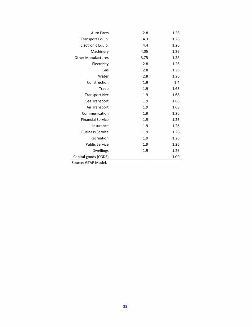
Appendix A. Key Elasticity Parameters in the GTAP Model

Table A. Various Elasticities of Substitutions Adopted in the GTAP Model

Sector Armington elasticity of substitution

Factor elasticity of substitution

Paddy Rice 5.05 0.26 Wheat 4.45 0.26

Cereal Grains 1.3 0.26 Vegetables 1.85 0.26

Oil Seeds 2.45 0.26 Sugar Cane 2.7 0.26 Plant Fibers 2.5 0.26

Crops 3.25 0.26 Cattle 2 0.26

Animal Products 1.3 0.26 Raw Milk 3.65 0.26 Wool Silk 6.45 0.26 Forestry 2.5 0.2

Fishing 1.25 0.2 Coal 3.05 0.2

Oil 5.2 0.2 Gas 17.2 0.2

Minerals 0.9 0.2 Meat 3.85 1.12

Meat Product 4.4 1.12 Vegetable Oil 3.3 1.12 Dairy Product 3.65 1.12

Processed Rice 2.6 1.12 Sugar 2.7 1.12

Food Products 2 1.12 Beverage & Tobacco 1.15 1.12

Textiles 3.75 1.26 Wearing Apparel 3.7 1.26 Leather Products 4.05 1.26

Wood Products 3.4 1.26 Paper 2.95 1.26

Petroleum 2.1 1.26 Chemical 3.3 1.26

Mineral Products 2.9 1.26 Ferrous Metals 2.95 1.26

Metals 4.2 1.26 Metal Products 3.75 1.26

35

Auto Parts 2.8 1.26 Transport Equip. 4.3 1.26 Electronic Equip. 4.4 1.26

Machinery 4.05 1.26 Other Manufactures 3.75 1.26

Electricity 2.8 1.26 Gas 2.8 1.26

Water 2.8 1.26 Construction 1.9 1.4

Trade 1.9 1.68 Transport Nec 1.9 1.68 Sea Transport 1.9 1.68 Air Transport 1.9 1.68

Communication 1.9 1.26 Financial Service 1.9 1.26

Insurance 1.9 1.26 Business Service 1.9 1.26

Recreation 1.9 1.26 Public Service 1.9 1.26

Dwellings 1.9 1.26 Capital goods (CGDS) 1.00

Source: GTAP Model.

36

Appendix B. Comparison of Trade between the U.S. and Korea to Overall Trade with the Rest of the World

In Table B1 and Table B2, we provide trade statistics to examine how specialized the trade

between the U.S. and Korea is compared to the each individual country’s overall trade with the

rest of the world (ROW). Table B1 presents the top 10 commodities that the U.S. imported

from Korea in 2014 dollar values. The proportion of each type of imported commodity with

respect to total imports from Korea is presented in the second numerical column. More than

two-thirds of the total imports from Korea are Motor Vehicles and Parts, Electrical Equipment,

and Industrial Machinery. This proportion is much higher than the percentage these three

types of commodities represent in total U.S. imports from the ROW, which is only 38% (see

Column 4 of Table B1). The last two columns of Table B1 present the dollar values of Korean

exports of these commodities to the ROW, as well as the percentages with respect to Korean

total exports to the ROW. The numbers indicate that Korea exports more Electrical Equipment

to ROW than to U.S. in percentage terms, but the U.S. has been the major exporting country for

Korean manufactured Motor Vehicles & Parts and Industrial Machinery.

Table B2 presents the trade data on the U.S. export-side (or Korea import-side). The first two

numerical columns present the top 10 U.S. exported commodities to Korea in dollar values and

their corresponding percentage with respect to total U.S. exports to Korea. The top 5

commodities are Industrial Machinery, Electrical Equipment, Aircraft, Precision Instruments,

and Oil & Mineral Fuels. Compared to the data presented in Columns 3 and 4, which pertain to

U.S. exports of these commodities to the ROW, the U.S. exports proportionally more Industrial

Machinery and Electrical Machinery, but less Oil & Mineral Fuels to Korea than to the ROW.

37

However, the difference between the trade with Korea and the trade with the ROW is not as

substantial as on the import-side. The last two columns of Table B2 present the dollar values of

Korea import of these commodities from the ROW, as well as the percentages with respect to

Korea total imports from the ROW. The numbers indicate that Korea imports more Electrical

Machinery and Oil & Mineral Fuels from the ROW than from the U.S. in percentage terms, but

more Industrial Machinery, Aircraft, and Precision Instruments from the U.S.

Table B1. Comparison of U.S. Imports from Korea vs. U.S. Imports from the ROW

Commodity (at 2-digit HTS level)

US Imports from Korea (Korea Exports to US) US Imports from ROW Korea Exports to ROW

billion $ % of total imports

from Korea billion $

% of total imports from

ROW billion $

% of total exports to

ROW

87 Motor Vehicles & Parts 19.4 27.9% 242.2 11.1% 43.2 12.6% 85 Electrical Equipment 15.5 22.2% 300.4 13.4% 118.8 27.1% 84 Industrial Machinery 11.5 16.5% 313.6 13.8% 46.7 11.8% 73 Iron & Steel Articles 3.3 4.8% 34.4 1.6% 7.8 2.2% 27 Oil & Mineral Fuels 3.0 4.4% 344.7 14.8% 24.5 5.5% 72 Iron & Steel 2.1 3.0% 32.1 1.5% 16.6 3.8% 39 Plastics 1.8 2.6% 46.1 2.0% 25.8 5.6% 40 Rubber 1.8 2.6% 25.8 1.2% 5.1 1.4% 29 Organic Chemicals 1.4 2.1% 52.2 2.3% 16.5 3.6% 90 Precision Instruments 1.1 1.6% 74.3 3.2% 26.5 5.6%

38

Table B2. Comparison of U.S. Exports to Korea vs. U.S. Exports to the ROW

Commodity (at 2-digit HTS level)

US Exports to Korea (Korea Imports from US) US Exports to ROW Korea Imports from ROW

billion $ % of total exports to

Korea billion $

% of total exports to

ROW billion $

% of total imports from

ROW

84 Industrial Machinery 7.6 17.1% 212.3 13.5% 38.4 10.6% 85 Electrical Equipment 5.9 13.3% 166.4 10.6% 69.2 19.1% 88 Aircraft 2.9 6.4% 122.4 7.8% 1.2 0.3% 90 Precision Instruments 2.9 6.4% 82.1 5.2% 14.6 4.0% 27 Oil & Mineral Fuels 2.0 4.4% 154.5 9.8% 79.8 22.0% 29 Organic Chemicals 1.9 4.2% 40.4 2.6% 9.1 2.5% 87 Motor Vehicles & Parts 1.6 3.6% 134.4 8.5% 13.6 3.8% 39 Plastics 1.6 3.5% 61.6 3.9% 8.5 2.3% 10 Cereals 1.5 3.4% 21.3 1.4% 1.7 0.5% 02 Meat 1.4 3.1% 16.3 1.0% 2.5 0.7%

39

Appendix C. Real GDP Changes for the Top Negatively US-Korea FTA Affected Sectors

We examined the percentage changes in sectoral real GDP of the three sectors that are

predicted to be most negatively affected by the US-Korea FTA over the period of 2012 to 2015

to evaluate whether there is empirical evidence to indicate whether the findings from our GTAP

simulations for the year 2014 were aberrations or not. Table C indicates that the Machinery

Manufacturing sector has been experiencing a decline in sectoral GDP over the three years

after the implementation of the FTA. Although the GDP of the Motor Vehicles and Parts

Manufacturing sector has been increasing over the years, there has been a decrease in the

growth rate. Between 2014 and 2015, the sectoral GDP growth rate (0.2%) is much lower than

the weighted average GDP growth rate (2.7%) across all sectors in the U.S. The Electronic

Equipment Manufacturing sector had a similar GDP growth rate as the sectoral weighted

average over the years. Therefore, the GDP data of these three sectors support our findings

from the GTAP simulations to some extent: although some sectors are predicted to be

negatively affected by the US-Korea FTA, overall, the U.S. economy benefits from the FTA.

However, we reiterate that we are performing a comparative static analysis, which only

examines the difference made by the US-Korea FTA, holding all the other economic conditions

constant. The changes in sectoral GDP presented in Table C can be caused by multiple

economic factors, which are difficult to separate out from the impacts of the US-Korea FTA.

40

Table C. Percent Real GDP Change from Preceding Year for the Top Three Negatively Impacted Sectors

2013 2014 2015 Motor Vehicles and Parts Manufacturing 5.1 4.3 0.2 Electronic Equipment Manufacturing 0.8 2.5 3.5 Machinery Manufacturing -1.8 -0.3 -8.7 Total U.S. 1.5 2.4 2.7