Embed Size (px)
Citation preview

Working Paper Series, Paper No. 11-12
Estimating economic impact using ex post econometric analysis:
Cautionary tales
Robert Baumann† and Victor A. Matheson
††
May 2011
Abstract
This paper provides an overview of techniques that can be used to estimate the economic
impact of stadiums, events, championships, and franchises on local economies. Utilizing data
from National Collegiate Athletic Association championships, this paper highlights the potential
problems that can be made if city and time effects are not handled and unit-roots are not
accounted for. In addition, the paper describes the technique for estimating dynamic panel data
and the advantages that come with these modeling techniques.
JEL Classification Codes: L83, R53, C23
Keywords: College sports, impact analysis, econometrics
†Robert Baumann, Department of Economics, Box 192A, College of the Holy Cross,
Worcester, MA 01610-2395, 508-793-3879 (phone), 508-793-3708 (fax),
††Victor A. Matheson, Department of Economics, Box 157A, College of the Holy Cross,
Worcester, MA 01610-2395, 508-793-2649 (phone), 508-793-3708 (fax),

1
Introduction
Since the seminal work of Baade and Dye (1988) over twenty years ago, the analysis of the
economic impact of sports teams, stadiums, and major athletic events on host economies has
elicited significant attention from sports economists. There are two main reasons. First, the topic
has considerable public finance implications. Over the past two decades over 100 stadium and
arena construction projects have taken place at a cost totaling in excess of $30 billion in the U.S.
and Canada alone (Baade and Matheson, 2011). Since over half of this cost has been borne by
state and local governments, it is reasonable to ask whether taxpayers are getting a good return
on their investment.
The second reason for the consideration is the clear difference between the ex ante
economic benefit estimates provided by economists working in a consulting capacity at the
behest of sports organizers and the ex post estimates provided by economists working in a
scholarly setting. Ex ante economic impact numbers are typically generated by predicting the
number of visitors to an event and the average spending per visitor. Multiplying these two
figures together provides an estimate of the direct economic impact. A multiplier is then applied
to the direct economic impact to arrive at an estimate of total economic impact. Invariably the
total economic impact of sports teams and events estimated in this manner is extremely
impressive.
Critics of this process point out several flaws in this methodology. First, ex ante
economic impact reports tend to report the gross rather than the net economic impact of spectator
sports. Local residents who spend their money on sports have less disposable income to spend on
other goods and services in the local economy. Sports may simply shift spending around but not
cause an increase in local incomes. Similarly, sports fans may displace other consumers. Finally,

2
the multipliers used are often implausibly large, and even when reasonable looking multipliers
are used, rarely do they account for the unique circumstances that surround professional sports
(Matheson, 2009; Siegfried and Zimbalist, 2002).
In order to test the effects of these theoretical deficiencies, numerous researchers have
followed Baade and Dye (1988) including Coates and Humphreys (1999; 2002), Baade and
Matheson (2002, 2004), Baade, Baumann, and Matheson (2008), Hagn and Maennig (2008),
Jasmand and Maennig (2008), and Feddersen and Maennig (2010) to name just a few. These
economists have performed ex post analyses of the performance of economic variables in local
economies in the wake of new stadium construction, mega-events, and franchise relocation. An
ex post evaluation of economic impact examines some aspect of a local economy such as
personal income, employment, income per capita, taxable sales, or visitor arrivals, and compares
the data before, during, and after an event, new stadium construction, or franchise move. If the ex
ante estimates are correct, then shifts of a similar magnitude should be observable in the data. In
fact, these types of studies have typically found that sporting events, teams, and stadiums create a
fraction of the economic benefits predicted in ex ante studies.
While the flaws of ex ante studies are clear, it is also easy for errors to be made in ex post
economic impact analyses. The purpose of this paper is to highlight what types of errors can be
made in ex post analyses and to explain the intuition behind why such errors occur.
Data
In order to motivate the discussion of potential econometric errors and to provide
concrete examples, this paper will utilize a time series cross section (a.k.a. a dynamic panel) data
set on college athletics in the United States. The National Collegiate Athletic Association

3
(NCAA) is the largest governing body for intercollegiate sports in the U.S. With nearly 1,100
member schools, the organization serves as both a rule-making body as well as the primary
sponsor for championships in intercollegiate sports among its members. While several other
collegiate athletic associations exist, including the 290-member National Association of
Intercollegiate Athletics, and the roughly 500-member National Junior College Athletic
Association, the NCAA is both the largest and most prominent organization, and its members
also include the biggest and most highly funded athletic programs in the country. The NCAA
categorizes its member schools into one of three divisions based on school size, recruiting rules,
athlete eligibility, and the availability of scholarship money for athletes. Division I is the highest
level of competition and comprises 338 schools ranging from large state universities to smaller
private colleges. The NCAA sponsors championships in 37 different sports, including the
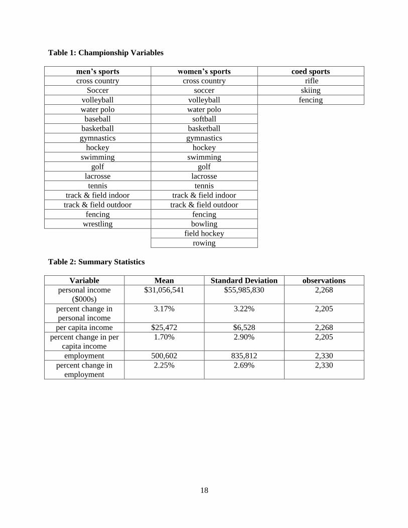
different championships held for men and women athletes in most sports. Table 1 lists the sports
with a championship. Football was excluded from the sample of national championships since
the national championship in football for the top schools is not administered by the NCAA, and
the “true” national champion is the source of some dispute and three other sports.
This paper uses data from 1969 through 2005 for 60 metropolitan areas that are home to a
university with a football team belonging one of the six major Division I athletic conferences in
the country. In addition, Provo, Utah, Colorado Springs, Colorado, and South Bend, Indiana,
homes to Brigham Young, Air Force, and Notre Dame, respectively, are added to the sample
bringing the total number of cities examined up to 63. While the list of cities in the sample is
somewhat ad hoc, the sample covers the home city for the majority of universities that one would
normally consider to have a major athletic program. Indeed, schools in these cities account for
just under 800 of the 995 national championships awarded in various sports by the NCAA during

4
this time period. Restricting the sample to these major athletic programs provides for a
manageable data set and ensures that the host city is large enough be including within one of the
Census Department’s defined metropolitan statistical areas (MSAs). In most cases, only a single
major university resides in each MSA; however, in some cases, notably Los Angeles, two or
more Division 1 may have won national championships and no differentiation is made for which
school within an MSA was named champion. For each MSA, we have data on total personal
income, per capita income, and employment. Table 2 presents the summary statistics to the
levels and percent changes of all three variables. The only caveat is that our sample frame ends at
2005 for employment and 2004 for personal income and per capita income. We merge these
economic data with the championship information to create dummy variables for each champion
in a given year.
Up to this point, the data assembled is similar to that used in many other ex post analyses
of the economic impact of sports. What is of crucial importance here, however, is that there is no
conceivable mechanism by which national championships in the vast majority of NCAA
Division 1 sports can have any meaningful impact on MSA-wide economic variables. Outside
of football, which is not examined in this study, and men’s basketball, most intercollegiate sports
have relatively few followers. National championships are low budget, sparsely attended events
that generate little media coverage. In addition, most national championships are held at neutral
venues, so the winner of a national championship will typically not benefit from any tourism
inflows, even small though they may be, nor do winning teams receive any monetary rewards
from the NCAA. Therefore, any economic impact would have to rely on psychological effects on
local workers, capital or labor inflows as a result of an advertising effect, or other indirect
factors. While Coates and Humphries (2002), and Davis and End (2010) suggest that

5
psychological factors may be at work in explaining an identified increase in economic activity
among cities that win the Super Bowl in the National Football League, such an explanation for
championships in minor college sports borders on the absurd. In fact, should winning a
championship in any of the sports examined in this paper turn out to have a significant effect on
any of the MSA economic variables, the only logical conclusion to draw is one of spurious
correlation or model misspecification. The results of this paper will show how easy it is to end up
with statistically significant results for minor sporting events given incorrect econometric
modeling.
Models I and II: Levels without fixed effects for years or MSAs
Given we have data for 63 MSAs over 36 (1969-2004 for personal income and per capita
income) or 37 (1969-2005 for employment) years, we begin by using panel data techniques to
account for time-invariant effects of each MSA. While we have the alternative of estimating
separate models for each MSA, as is done in Baade and Matheson (2004), we lose the control
group of the remaining MSAs. However, pooling data into a panel also makes heteroskedasticity
far more likely. We include panel-corrected standard errors to allow the error variance to be
different across MSAs. Whether the data are pooled or not, it is likely autocorrelation exists
within each MSA. We will return to this issue later in the paper.
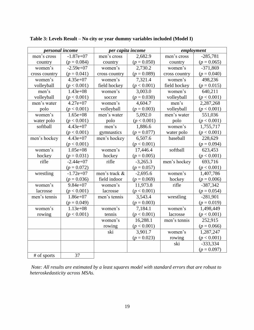
Ignoring for now the potential problem of unit roots, which are almost certain to exist
when dealing with time series involving economic data in levels, Table 3 presents only the
statistically significant estimates in a least squares model with the championship variables as the
only covariates. The insignificant controls are available upon request. At this point, MSA-level
fixed effects and yearly dummies are not included. Table 3 shows that nearly half (47 out of 99

6
total) of the championship dummy variables are statistically significant across the three
dependent variables. As stated previously, the only explanations for statistically significant
championship variables are spurious correlations and/or model misspecification.
In most sports, team quality is likely to persist over a long period of time due to coaching
quality, program reputation, and/or institutional support, and therefore championships are
commonly dominated by a small number of schools. If these universities happen to be located in
MSAs with an above (below) average level of income, employment, or per capita income, then
the championships in those sports will show up as being correlated to high (low) incomes, etc.
For example, West Virginia University (WVU) has won half of the NCAA rifle championships
in our sample. WVU is located in Morgantown, West Virginia, a town that is both significantly
smaller and poorer that the typical “college town” in the data set. The negative coefficients on
income, personal income, and employment for the rifle championships in Table 3 clearly reflect
the size and wealth of Morgantown rather than the influence of perhaps the smallest of all NCAA
championship sports. Similarly, teams from the Los Angeles MSA have dominated men’s and
women’s water polo and men’s volleyball leading to highly statistically significant results on
employment and personal income for these championships.
Indeed, the necessity of including city effects places a major constraint on the types of
events that can be examined using ex post econometric analysis. Standard ex post techniques can
only examine variables in which there is some type of movement between cities since the
inclusion of city-level fixed effects causes perfectly collinearity between the fixed effect and the
event dummy variable. For example, the Super Bowl can be examined because it changes
location every year, but major college football bowl games such as the Rose Bowl cannot be
easily studied since the game takes place in the same city on the same day every year. Even if

7
one observes a large surge in spending in Pasadena every New Year’s Day, it would be nearly
impossible to disentangle whether the boost in economic activity was due to the Rose Bowl or
other unique features of the Pasadena economy on that day. Similarly, studies of stadiums and
arenas must concentrate on changes in sports infrastructure, such as new stadiums or renovations
to existing facilities, rather than on the potential impact of existing stadiums.
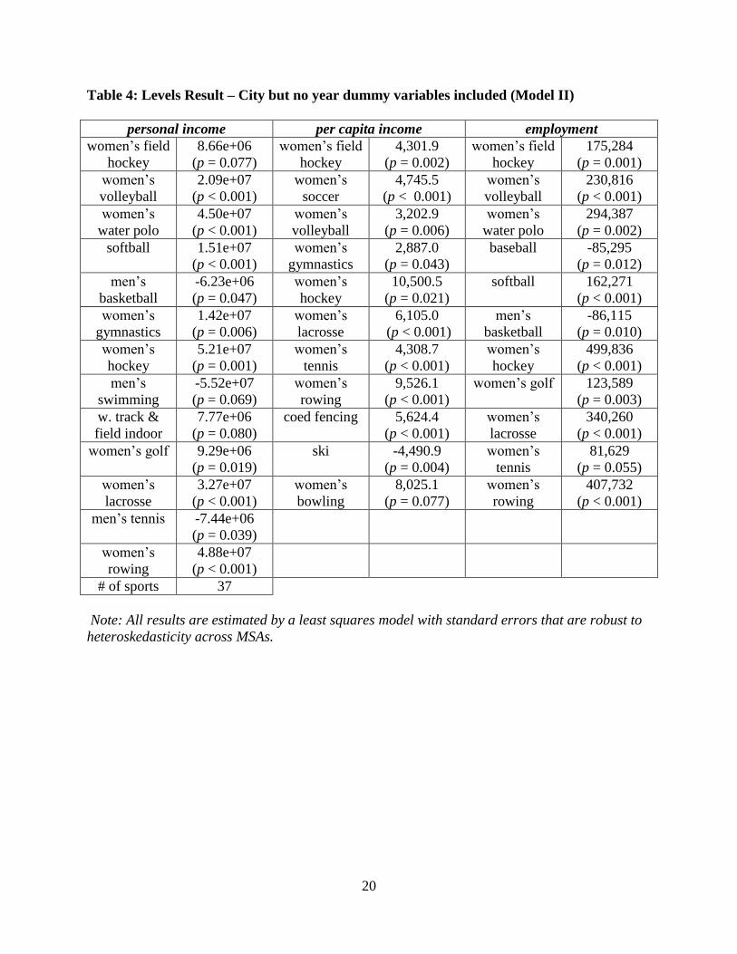
It is also not sufficient to account only for differences between cities. Table 4 shows
statistically significant estimates in least squares estimations on all three dependent variables but
includes MSA-level fixed effects. Again, many championship dummy variables are statistically
significant particularly in women’s sports, which constitute 28 of the 35 significant
championship variables across the three estimations. Given the NCAA did not begin to sponsor
championships in women’s sports until 1981, this finding is likely the byproduct of the upward
trend in each dependent variable. Similar spurious correlations are likely if time trends are not
properly accounted for when examining the economic impact of any sport in which team or
playoff expansion has occurred or the number of games played per season has changed.
Model III: Levels
Even when MSA-level fixed effects and yearly dummies are included, many economic
variables are almost certain to have a unit root given a reasonable time period. Using Dickey-
Fuller and Phillips-Perron tests, our three dependent variables – per capita income, personal
income, and employment – fail all MSA-specific unit root tests except in one case: Pullman,
WA, which is the home of Washington State University. This MSA rejects the existence of a unit
root for personal income in both Dickey-Fuller and Phillips-Perron tests. The unit roots in all

8
MSAs but one are almost certainly a result of the upward trend in all three dependent variables
over our time frame.
We also execute three time series panel unit root tests: Hadri (2000), Levin, Lin, and Chu
(2002) and Im, Pesaran, and Shin (2003). These tests differ by their flexibility when faced with
other econometric problems. For example, Hadri (2000) allows for heteroskedasticity, which is
common in time-series panels. Im, Pesaran, and Shin (2003) and Levin, Lin, and Chu (2002)
allows for an overall time trend and also MSA-specific fixed effects and time trends. All three
tests suggest a unit root is present in each of our three independent variables.
Table 5 presents only the statistically significant estimates in estimations on all three
dependent variables. Although not presented, MSA-level fixed effects and yearly dummies are
included. Those results are available upon request. Including MSA-level fixed effects and yearly
dummies forces us to omit four championships – women's bowling (Nebraska), men's fencing
(Notre Dame), rifle (W. Virginia), and women's hockey (Minnesota) – which we observe in only
one year or only one champion. As stated above, the only explanations for statistically significant
championship variables are spurious correlations and/or model misspecification. Table 3 shows
statistically significant championship controls at 1.0 : six in the per capita income estimation,
seven in the personal income estimation, and ten in the employment estimation. Given there are
33 championship variables, such a high percentage of significant variables is almost certainly the
fault of the unit root caused by the upward trend of each dependent variable. Of these 23
significant estimates, 14 are positive. Though not presented at Table 5, it is also worth noting
that nearly all of the year dummies are statistically significant with an upward trend except for
recessions during the time frame.
9
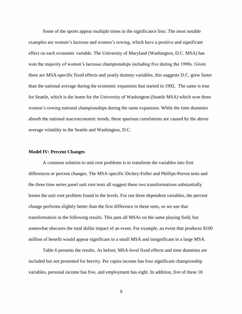
Some of the sports appear multiple times in the significance lists. The most notable
examples are women’s lacrosse and women’s rowing, which have a positive and significant
effect on each economic variable. The University of Maryland (Washington, D.C. MSA) has
won the majority of women’s lacrosse championships including five during the 1990s. Given
there are MSA-specific fixed effects and yearly dummy variables, this suggests D.C. grew faster
than the national average during the economic expansion that started in 1992. The same is true
for Seattle, which is the home for the University of Washington (Seattle MSA) which won three
women’s rowing national championships during the same expansion. While the time dummies
absorb the national macroeconomic trends, these spurious correlations are caused by the above
average volatility in the Seattle and Washington, D.C.
Model IV: Percent Changes
A common solution to unit root problems is to transform the variables into first
differences or percent changes. The MSA-specific Dickey-Fuller and Phillips-Perron tests and
the three time series panel unit root tests all suggest these two transformations substantially
lessen the unit root problem found in the levels. For our three dependent variables, the percent
change performs slightly better than the first difference in these tests, so we use that
transformation in the following results. This puts all MSAs on the same playing field, but
somewhat obscures the total dollar impact of an event. For example, an event that produces $100
million of benefit would appear significant in a small MSA and insignificant in a large MSA.
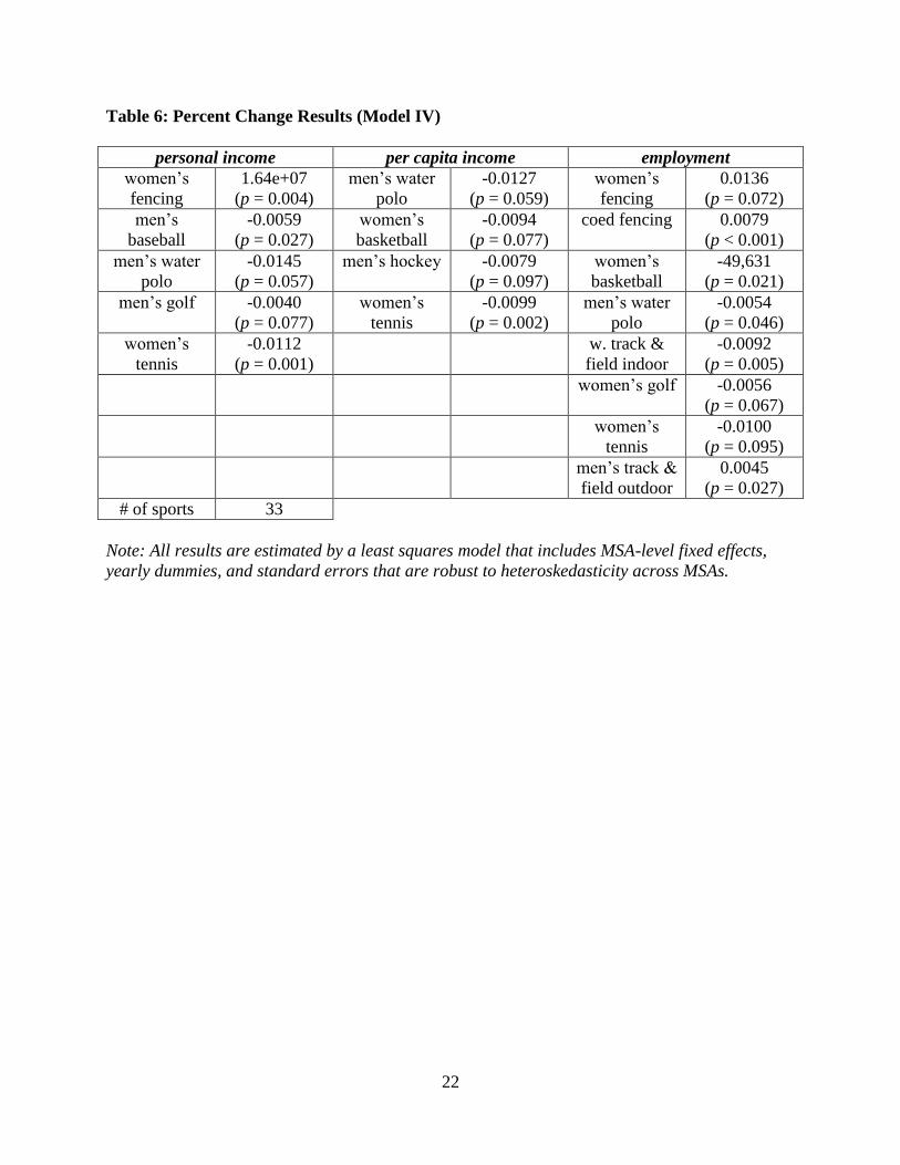
Table 6 presents the results. As before, MSA-level fixed effects and time dummies are
included but not presented for brevity. Per capita income has four significant championship
variables, personal income has five, and employment has eight. In addition, five of these 18

10
significant variables are positive. These percentages of significance and positive significance are
more in line with the random spurious correlations though not a perfect fit. Assuming no model
misspecification, the expected number of randomly significant variables is 10 (compared to our
18) given a ten percentage threshold for significance and 33 championship variables in three
estimations.
Similar the levels estimations, some of the sports appear multiple times in the
significance lists. Women’s tennis is negative and significant for all three economic variables,
while men’s tennis is negative and but near significance (p-values of 0.188 and 0.302) in two of
three. Stanford University (San Jose-Sunnyvale-Santa Clara MSA) is a dominant program in
both men’s and women’s tennis. However, most of its women’s tennis championships occur
during recessions including championships during the early 1980s, early 1990s, and early 2000s.
Meanwhile, their men’s team tended to win during expansions, most notably six during the
1990s. In addition, the economy of the San Jose-Sunnyvale-Santa Clara MSA is more volatile
than the rest of the nation. For that MSA, each economic variable has a standard deviation at
least 50% higher than the national average. We conclude these significant championship
variables are a result of this volatility.
Model V: Instrumental Variables-General Method of Moments Models
Models I through IV treat the data as if it were a panel, but it could be argued our data
more resemble a time series cross section (TSCS), which is also called a dynamic panel. Much
has been written about the difference, but the main issues are whether “T is large enough to do
serious averaging over time, and also whether it is large enough to make some econometric
problems disappear” (Beck and Katz, 2004, p. 3). Given T = 35 in our data set, this likely passes

11
the threshold mentioned by Beck and Katz which means we are probably better off using
techniques designed for TSCS data. In addition, we use no explanatory variables to control for
the macroeconomy other than MSA-level fixed effects and yearly dummies. Part of this rationale
is avoiding the likely endogeneity that is caused by including another macro control. But this
means the error term includes a greater amount of information, and this information is almost
certain to be correlated over time within an MSA. In other words, it is highly likely Models I and
II suffer from autocorrelation.
On autocorrelation test appears in Wooldridge (2002), where the null hypothesis is no
autocorrelation. We perform this test for each of our 63 MSAs since it is not appropriate for
TSCS data. For our three dependent variables, 55 (personal income), 52 (per capita income), and
61 (employment) of 63 reject the null hypothesis of no autocorrelation at 1.0 . Since
autocorrelation produces incorrect standard errors, our significance tests in models I and II are
suspect.
One solution to removing the inertia in the error is to include the lagged dependent
variable as a regressor. Unfortunately, this addition biases the fixed effect estimators because the
that model is equivalent to a least squares estimation that transforms the data to deviations of
MSA-specific means. It is these means that create a correlation between the independent
variables and the error term. As N approaches infinity, Nickell (1981) shows the amount of
inconsistency is of order 1T . This may seem small given T = 35 in our sample, but N = 63 is not
nearly close enough to infinity to assume this result.
There are two solutions to produce consistent estimates in this framework. One option is
to choose a technique from the Instrumental Variable-General Method of Moments (IV-GMM)
family of estimators, which include Anderson and Hsiao (1982), Arellano and Bond (1991), and
12
Blundell and Bond (1998). All three methods first difference the equation and use past
information about the lagged dependent variable as instruments for the lagged dependent
variable, i.e. the endogenous regressor. The main difference between Anderson and Hsiao (1982)
and Arellano and Bond (1991) is the level of identification. Anderson and Hsiao (1982) propose
an exactly identified IV strategy that uses the second lag to instrument for the endogenous first
lag. In comparison, the Arellano and Bond (1991) technique is over-identified because the
researcher can use as many higher-order lags as the data will allow. Blundell and Bond (1998)
propose a different estimator for small-sample cases which are more likely to produce weak
instruments. One advantage of all of these methods is that any potentially endogenous
independent variable can be instrumented in the same way.
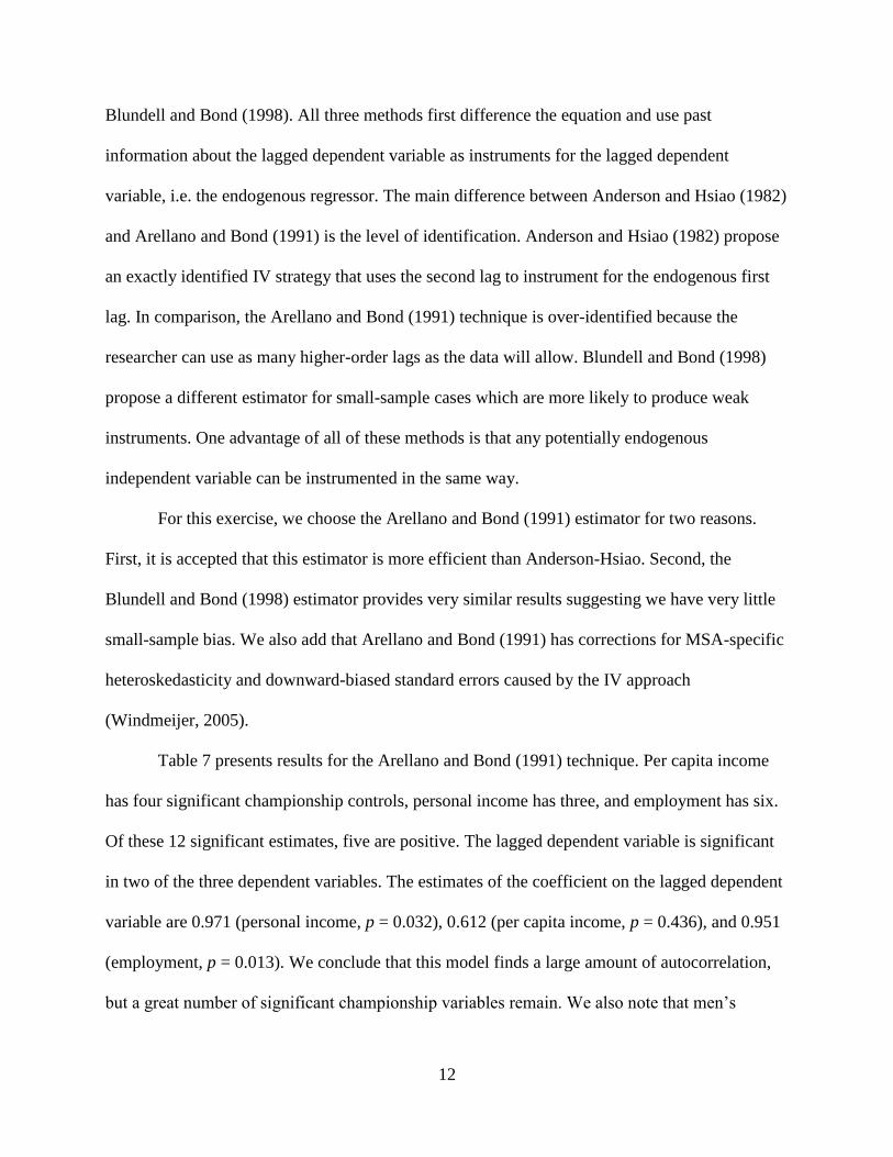
For this exercise, we choose the Arellano and Bond (1991) estimator for two reasons.
First, it is accepted that this estimator is more efficient than Anderson-Hsiao. Second, the
Blundell and Bond (1998) estimator provides very similar results suggesting we have very little
small-sample bias. We also add that Arellano and Bond (1991) has corrections for MSA-specific
heteroskedasticity and downward-biased standard errors caused by the IV approach
(Windmeijer, 2005).
Table 7 presents results for the Arellano and Bond (1991) technique. Per capita income
has four significant championship controls, personal income has three, and employment has six.
Of these 12 significant estimates, five are positive. The lagged dependent variable is significant
in two of the three dependent variables. The estimates of the coefficient on the lagged dependent
variable are 0.971 (personal income, p = 0.032), 0.612 (per capita income, p = 0.436), and 0.951
(employment, p = 0.013). We conclude that this model finds a large amount of autocorrelation,
but a great number of significant championship variables remain. We also note that men’s

13
basketball, which has a positive and significant effect on employment, cannot be ruled out as
spurious because of its high profile.
Models VI and VII: Lagged Dependent Variable Models
While introducing a lagged dependent variable allows us to model autocorrelation, the IV
correction can produce several unintended consequences especially if the instruments are weak
or the sample is small. Kiviet (1995) and later Bruno (2005) take a different path by first
estimating the amount of bias in a lagged dependent variable model that does not correct its
endogeneity. Once the bias is estimated, it adjusts the estimates. This result is inspired by Nickell
(1981), who first derived the amount of inconsistency in these models.
The Monte Carlo evidence tends to favor the Kiviet correction to IV-GMM models (see
Judson and Owen, 1999; Bun and Kiviet, 2003; Bruno, 2004), but there are two other issues with
the Kiviet correction. First, its bias correction formula includes the parameter values of the
autoregressive coefficient and the error variance. Since these are unobservable, Kiviet (1995)
recommends using consistent estimates from either the Anderson-Hsiao, Arellano-Bond, or
Blundell-Bond techniques. Although all of these produce consistent estimates, sample sizes in
macroeconomic data tend to be small and this introduces extra noise in the estimation. Second,
there is only an asymptotic formula for the standard errors (see Bun and Kiviet, 2001). Bruno
(2005) outlines a bootstrap technique based on the normal distribution that we use here.
Beck and Katz (2004) argue a Kiviet correction to a lagged dependent variable model
may not even be necessary. Their Monte Carlo evidence that suggests omitting a Kiviet
correction given T > 20 since there is little difference in bias and mean squared error above this
threshold. However, they also find the Kiviet correction produces a lower mean squared error in
14
cases with high autocorrelation, which is what the results from the Model 3 suggest. For this
reason, we include estimates with and without the Kiviet correction. Since least squares is well
known to produce inconsistent estimates in models with lagged dependent variables, we estimate
the “without Kiviet” models with maximum likelihood. Finally, we use robust standard errors to
guard against heteroskedasticity across MSAs.
Table 8 lists the significant championship variables using the Kiviet-corrected technique,
and Table 9 presents the same for the maximum likelihood estimation, i.e. no Kiviet correction.
Both estimations produce 11 significant championship variables, and some of the sports overlap.
The significant controls are also more likely to be negative than positive. Of the 22 significant
estimates, eight are positive. There are also similarities in the autoregressive term estimates. For
the personal income and employment estimations, the Kiviet and lagged dependent variable
models produce very similar and highly significant estimates of the AR process. In the per capita
income model, this term is insignificant. We also note the autoregressive component is closer to
zero in these models compared to the Arellano-Bond approach.
The results of models VI and VII are both reassuring and highlight an inherent problem
in statistical inference. With only 11 significant championship variables, each model produces
roughly the number of significant results that one would normally expect from a regression with
99 independent sports variables suggesting that the modeling technique has been largely
successful at eliminating spurious correlation. On the other hand, an unsophisticated reading of
the results may lead one to believe that the 11 remaining sports with statistically significant
championship coefficients really are driving economic growth rather than being the result of pure
chance. Of course, an economic policy using the promotion of women’s collegiate fencing as a
tool to spur economic growth is likely to be a spectacular failure. It is important to remember that

15
researchers should resist placing too much emphasis a single econometric result in any
estimation that utilizes a large vector of sports-related variables.
Conclusions
Economic impact studies are vital to the literature and public policy debates. While the
academic literature agrees that ex post studies produce better estimates than ex ante approaches,
there is no consensus on the right empirical techniques. Part of this problem is data specific. In
this paper, we consider methods for data with multiple time observations for multiple geographic
areas, which are known as dynamic panels or time-series cross-sections. We build an
econometric model where NCAA championships can impact one of three economic indicators
based on the assumption that a championship outside of the two highest profile sports (football
and men’s basketball) should have no economic impact. We reach the following conclusions:
First, both city and time effects must be considered which limits the number and type of
events that can be examined using ex post analysis. Second, unit roots are a major problem. At a
minimum, economic impact studies require a long enough time period to map out the “typical”
path of the economic indicator. Any length that accomplishes this is almost certain to have an
upward trend and ignoring this problem produces many spurious correlations. In addition, since
there has been an increase in the number of NCAA sports over our sample, we find a high
number of significant and positive championship effects in our estimations that are almost
certainly false. Such problems will also occur in any league that has experienced expansion or an
increase in the number of contests played per season.
The common solutions to unit root problems, namely first differencing and percent
changes, are the right antidote but there are important implications to both especially when the

16
variance of the dependent variables across groups is high. A percent change approach will put
different groups on a level playing field. In our data, a percent change means that any impact on,
say, Ames, Iowa (home of Iowa State University) is comparable to a much larger MSA like Los
Angeles (home of both University of Southern California and University of California Los
Angeles). However, if the event is speculated to have a constant impact across MSAs, say $400
million for hosting a Super Bowl, then first differences are more direct.
Third, fixed effects (and to a lesser extent time dummies) cure some econometric
problems but also create others. Since geographic areas follow different growth paths, a fixed
effect purges time-invariant growth factors. This also lessens – but usually does not eliminate –
heteroskedaticity. Time dummies absorb macroeconomic effects that impact all of the
geographic areas, which will purge some generic business cycle problems from the data.
Unfortunately, fixed effects create biased estimates in a model with autocorrelation via the de-
meaning process of the data.
Fourth, the solution for autocorrelation is complicated, and in some cases the researcher
may be better off ignoring this problem than correcting it. Since the autocorrelation creates the
endogeneity that biases the estimates, one answer is an instrumental variable approach (i.e., IV-
GMM). The advantage of these techniques is they do not require the researcher to search for
instruments as they are embedded in the data. However, it is not assured that higher-order lags
will be good instruments. The Kiviet correction offers an alternative approach that is usually
preferred to IV-GMM estimators in Monte Carlo settings, but relies on the initial values set by an
IV-GMM model which may be improperly specified. Because of this ambiguity, Beck and Katz
(2004) argue that simply including a lagged dependent variable as a regressor or in some cases
ignoring autocorrelation altogether with a simple fixed effects estimator may be preferable. After

17
all, it is usually better to have inefficient estimates (i.e., ignoring autocorrelation) than biased
ones (i.e., using an improper fix). This is especially true for TSCS data with “larger” T, say T >
30. We feel that corrections for autocorrelation should consider all of the above approaches. In
our models, these techniques decrease the percentage of significant championship variables
which is an indicator that models that recognize autocorrelation are closer to the true result for
our data.
Fifth, the effect of an event or championship need not be in only one period. In our
examples, we consider a one-year bump to winning a championship since our a priori
assumption in these models is that championship variables should be insignificant. However,
there are other contexts where the effect of the event is felt for several periods following the
event. For example, Baade, Baumann, and Matheson (2008) find the effect of Hurricane Andrew
on Miami MSA was initially negative right after the storm and then positive as rebuilding efforts
began.
Finally, the only cure for spurious correlations is a well-specified model since economic
impact studies have serious potential for omitted variable bias. Most often an event is measured
as a simple dummy variable in the period it occurred, but clearly some other large event may be
the true driver of the effect. In fact, the ability to isolate the economic impact of some event is
another reason why fixed effects and time dummies are so important to these studies. This
problem increases with the length of the time period, i.e. monthly versus yearly data. Since none
of our techniques eliminate all of the significant championship variables, we echo the advice that
is in Austin, Mamdani, Juurlink, and Hux (2006) who warn against “the hazards of testing
multiple, non-prespecified hypotheses” (p. 968).
18
Table 1: Championship Variables
men’s sports women’s sports coed sports
cross country cross country rifle
Soccer soccer skiing
volleyball volleyball fencing
water polo water polo
baseball softball
basketball basketball
gymnastics gymnastics
hockey hockey
swimming swimming
golf golf
lacrosse lacrosse
tennis tennis
track & field indoor track & field indoor
track & field outdoor track & field outdoor
fencing fencing
wrestling bowling
field hockey
rowing
Table 2: Summary Statistics
Variable Mean Standard Deviation observations
personal income
($000s)
$31,056,541 $55,985,830 2,268
percent change in
personal income
3.17% 3.22% 2,205
per capita income $25,472 $6,528 2,268
percent change in per
capita income
1.70% 2.90% 2,205
employment 500,602 835,812 2,330
percent change in
employment
2.25% 2.69% 2,330
19
Table 3: Levels Result – No city or year dummy variables included (Model I)
personal income per capita income employment
men’s cross
country
-1.87e+07
(p = 0.084)
men’s cross
country
2,682.9
(p = 0.050)
men’s cross
country
-285,781
(p = 0.065)
women’s
cross country
-2.59e+07
(p = 0.041)
women’s
cross country
2,730.2
(p = 0.089)
women’s
cross country
-371,869
(p = 0.040)
women’s
volleyball
4.35e+07
(p < 0.001)
women’s
field hockey
7,321.4
(p < 0.001)
women’s
field hockey
498,236
(p = 0.015)
men’s
volleyball
1.43e+08
(p < 0.001)
women’s
soccer
3,003.0
(p = 0.030)
women’s
volleyball
640,211
(p < 0.001)
men’s water
polo
4.27e+07
(p < 0.001)
women’s
volleyball
4,604.7
(p = 0.003)
men’s
volleyball
2,287,268
(p < 0.001)
women’s
water polo
1.65e+08
(p < 0.001)
men’s water
polo
5,092.0
(p < 0.001)
men’s water
polo
551,036
(p < 0.001)
softball 4.43e+07
(p < 0.001)
men’s
gymnastics
1,886.6
(p = 0.077)
women’s
water polo
1,755,717
(p < 0.001)
men’s hockey 4.43e+07
(p < 0.001)
men’s hockey 6,507.6
(p < 0.001)
baseball 228,629
(p = 0.094)
women’s
hockey
1.05e+08
(p = 0.031)
women’s
hockey
17,446.4
(p = 0.005)
softball 623,453
(p < 0.001)
rifle -2.44e+07
(p = 0.072)
rifle -3,265.3
(p = 0.057)
men’s hockey 693,716
(p < 0.001)
wrestling -1.72e+07
(p = 0.036)
men’s track &
field indoor
-2,695.6
(p = 0.069)
women’s
hockey
1,407,786
(p = 0.006)
women’s
lacrosse
9.84e+07
(p < 0.001)
women’s
lacrosse
11,973.8
(p < 0.001)
rifle -387,342
(p = 0.054)
men’s tennis 1.86e+07
(p = 0.049)
men’s tennis 3,543.4
(p = 0.003)
wrestling -281,901
(p = 0.019)
women’s
rowing
1.13e+08
(p < 0.001)
women’s
tennis
7,184.1
(p < 0.001)
women’s
lacrosse
1,498,449
(p < 0.001)
women’s
rowing
16,288.1
(p < 0.001)
men’s tennis 252,915
(p = 0.066)
ski 3,901.7
(p = 0.023)
women’s
rowing
1,287,247
(p < 0.001)
ski -333,334
(p = 0.097)
# of sports 37
Note: All results are estimated by a least squares model with standard errors that are robust to
heteroskedasticity across MSAs.
20
Table 4: Levels Result – City but no year dummy variables included (Model II)
personal income per capita income employment
women’s field
hockey
8.66e+06
(p = 0.077)
women’s field
hockey
4,301.9
(p = 0.002)
women’s field
hockey
175,284
(p = 0.001)
women’s
volleyball
2.09e+07
(p < 0.001)
women’s
soccer
4,745.5
(p < 0.001)
women’s
volleyball
230,816
(p < 0.001)
women’s
water polo
4.50e+07
(p < 0.001)
women’s
volleyball
3,202.9
(p = 0.006)
women’s
water polo
294,387
(p = 0.002)
softball 1.51e+07
(p < 0.001)
women’s
gymnastics
2,887.0
(p = 0.043)
baseball -85,295
(p = 0.012)
men’s
basketball
-6.23e+06
(p = 0.047)
women’s
hockey
10,500.5
(p = 0.021)
softball 162,271
(p < 0.001)
women’s
gymnastics
1.42e+07
(p = 0.006)
women’s
lacrosse
6,105.0
(p < 0.001)
men’s
basketball
-86,115
(p = 0.010)
women’s
hockey
5.21e+07
(p = 0.001)
women’s
tennis
4,308.7
(p < 0.001)
women’s
hockey
499,836
(p < 0.001)
men’s
swimming
-5.52e+07
(p = 0.069)
women’s
rowing
9,526.1
(p < 0.001)
women’s golf 123,589
(p = 0.003)
w. track &
field indoor
7.77e+06
(p = 0.080)
coed fencing 5,624.4
(p < 0.001)
women’s
lacrosse
340,260
(p < 0.001)
women’s golf 9.29e+06
(p = 0.019)
ski -4,490.9
(p = 0.004)
women’s
tennis
81,629
(p = 0.055)
women’s
lacrosse
3.27e+07
(p < 0.001)
women’s
bowling
8,025.1
(p = 0.077)
women’s
rowing
407,732
(p < 0.001)
men’s tennis -7.44e+06
(p = 0.039)
women’s
rowing
4.88e+07
(p < 0.001)
# of sports 37
Note: All results are estimated by a least squares model with standard errors that are robust to
heteroskedasticity across MSAs.

21
Table 5: Levels Result – City and Year dummy variables included (Model III)
personal income per capita income employment
women’s
volleyball
1.64e+07
(p = 0.004)
men’s cross
country
1,401.8
(p = 0.059)
women’s
volleyball
177,180
(p = 0.004)
women’s
basketball
-5.52e+07
(p = 0.038)
men’s water
polo
-600.7
(p = 0.052)
women’s
basketball
-49,631
(p = 0.021)
women’s
water polo
3.694e+07
(p = 0.002)
women’s
soccer
1,633.8
(p = 0.010)
women’s
water polo
205,019
(p = 0.001)
men’s track &
field outdoor
-5.03e+06
(p = 0.075)
softball -772.2
(p = 0.086)
men’s water
polo
-23,633
(p = 0.089)
women’s
rowing
3.65e+07
(p < 0.001)
women’s
rowing
3,699.5
(p < 0.001)
women’s
rowing
275,948
(p < 0.001)
coed fencing -8.45e+06
(p = 0.007)
women’s
lacrosse
2,036.8
(p < 0.001)
women’s
soccer
-32,434
(p = 0.095)
women’s
lacrosse
2.47e+07
(p = 0.085)
women’s
lacrosse
244,984
(p = 0.045)
men’s
gymnastics
2.87e+06
(p = 0.036)
men’s track &
field outdoor
-53,724
(p = 0.019)
men’s
gymnastics
42,068
(p = 0.021)
coed fencing -84,500
(p 0.012)
# of sports 33
Note: All results are estimated by a least squares model that includes MSA-level fixed effects,
yearly dummies, and standard errors that are robust to heteroskedasticity across MSAs.
22
Table 6: Percent Change Results (Model IV)
personal income per capita income employment
women’s
fencing
1.64e+07
(p = 0.004)
men’s water
polo
-0.0127
(p = 0.059)
women’s
fencing
0.0136
(p = 0.072)
men’s
baseball
-0.0059
(p = 0.027)
women’s
basketball
-0.0094
(p = 0.077)
coed fencing 0.0079
(p < 0.001)
men’s water
polo
-0.0145
(p = 0.057)
men’s hockey -0.0079
(p = 0.097)
women’s
basketball
-49,631
(p = 0.021)
men’s golf -0.0040
(p = 0.077)
women’s
tennis
-0.0099
(p = 0.002)
men’s water
polo
-0.0054
(p = 0.046)
women’s
tennis
-0.0112
(p = 0.001)
w. track &
field indoor
-0.0092
(p = 0.005)
women’s golf -0.0056
(p = 0.067)
women’s
tennis
-0.0100
(p = 0.095)
men’s track &
field outdoor
0.0045
(p = 0.027)
# of sports 33
Note: All results are estimated by a least squares model that includes MSA-level fixed effects,
yearly dummies, and standard errors that are robust to heteroskedasticity across MSAs.

23
Table 7: Lagged Dependent Variables – Arellano-Bond (Model V)
personal income per capita income employment
women’s field
hockey
0.0143
(p = 0.055)
men’s water
polo
-0.0239
(p = 0.072)
women’s field
hockey
0.0049
(p = 0.075)
women’s
water polo
0.0788
(p = 0.033)
women’s
gymnastics
-0.0089
(p = 0.083)
football 0.0064
(p = 0.025)
women’s
gymnastics
-0.0111
(p = 0.076)
wrestling 0.0123
(p = 0.019)
men’s water
polo
-0.0090
(p = 0.038)
wrestling 0.0143
(p = 0.068)
women’s
tennis
-0.0099
(p = 0.002)
men’s
basketball
0.0084
(p = 0.012)
women’s
swimming
0.0192
(p = 0.015)
w. track &
field indoor
-0.0110
(p = 0.002)
men’s golf -0.0035
(p = 0.074)
women’s
lacrosse
0.0082
(p = 0.018)
Lags used as
instruments
2,3 Lags used as
instruments
3,4,5,6,7 Lags used as
instruments
2,3
Hansen over-
ident. test
2 0.30
(p = 0.584)
Hansen over-
ident. test
2 1.57
(p = 0.815)
Hansen over-
ident. test
2 0.14
(p = 0.708)
lagged dep.
var.
0.9708
(p = 0.032)
lagged dep.
var.
0.6125
(p = 0.436)
lagged dep.
var.
0.9511
(p = 0.013)
# of sports 33
Note: All estimations are done using the percent change of the dependent variable. The optimal
number of lags is determined using the Hansen (1982) over-identification test, which has a null
hypothesis of no over-identification.

24
Table 8: Lagged Dependent Variables – Kiviet Correction (Model VI)
personal income per capita income employment
men’s water
polo
-0.0146
(p = 0.006)
men’s water
polo
-0.0130
(p = 0.010)
men’s
basketball
0.0055
(p = 0.085)
men’s track &
field indoor
-0.0181
(p = 0.003)
men’s track &
field indoor
-0.0193
(p = 0.001)
men’s hockey -0.0090
(p = 0.093)
men’s track &
field outdoor
0.0092
(p = 0.092)
men’s tennis 0.0109
(p = 0.037)
men’s tennis 0.0112
(p = 0.025)
women’s
tennis
-0.0103
(p = 0.069)
women’s
tennis
-0.0101
(p = 0.062)
lagged dep.
var.
0.2143
(p < 0.001)
lagged dep.
var.
0.0267
(p = 0.202)
lagged dep.
var.
0.3823
(p < 0.001)
# of sports 33
Note: All estimations are done using the percent change of the dependent variable. We use the
Anderson-Hsiao method to obtain the consistent estimates necessary for the Kiviet Correction to
be calculated. The other IV-GMM techniques that produce consistent estimates (Arellano-Bond
& Blundell-Bond) do not substantially change the results. The variance-covariance matrix is
calculated using a bootstrap method over 500 iterations.

25
Table 9: Lagged Dependent Variables – MLE: No Kiviet Correction (Model VII)
personal income per capita income employment
men’s water
polo
-0.0156
(p = 0.013)
men’s water
polo
-0.0139
(p = 0.002)
men’s
basketball
0.0059
(p = 0.092)
men’s hockey -0.0115
(p = 0.005)
men’s hockey -0.0089
(p = 0.080)
men’s track &
field indoor
-0.0097
(p = 0.073)
women’s
fencing
0.0092
(p = 0.003)
men’s track &
field indoor
-0.0152
(p = 0.017)
men’s track &
field outdoor
0.0085
(p = 0.085)
men’s tennis 0.0107
(p = 0.018)
women’s
tennis
-0.0122
(p = 0.028)
lagged dep.
var.
0.2325
(p < 0.001)
lagged dep.
var.
0.0037
(p = 0.861)
lagged dep.
var.
0.3914
(p < 0.001)
# of sports 33
Note: All estimations are done using the percent change of the dependent variable. We use
maximum likelihood to calculate the estimates.

26
References
Anderson, T.W. and C. Hsiao (1981). “Formulation and Estimation of Dynamic Models Using
Panel Data,” Journal of Econometrics, Vol. 18, 570-606.
Arellano, M. and S.R. Bond. (1991). “Some Tests of Specification for Panel Data: Monte Carlo
Evidence and an Application to Employment Equations,” Review of Economic Studies,
Vol. 58, 277–297.
Austin, P.C., M.M. Mamdani, D.N. Juurlink, and J.E. Hux (2006). “Testing Multiple Statistical
Hypotheses Results in Spurious Associations: A Study of Astrological Signs and Health.”
Journal of Clinical Epidemiology, Vol. 59, 964-969.
Baade, R. and R. Dye (1988). “Sports Stadiums and Area Development: A Critical View,”
Economic Development Quarterly, Vol. 2:3, 265-275.
Baade, R., R. Baumann, and V. Matheson (2008) “Selling the Game: Estimating the Economic
Impact of Professional Sports through Taxable Sales,” Southern Economic Journal, Vol.
74:3, 794-810.
Baade, R. and V. Matheson (2002). “Bidding for the Olympics: Fool’s Gold?” (with Robert
Baade), in Transatlantic Sport: The Comparative Economics of North American and
European Sports, Carlos Pestana Barros, Muradali Ibrahimo, and Stefan Szymanski, eds.,
(London: Edward Elgar Publishing), 127-151.
Baade, R. and V. Matheson (2004). “The Quest for the Cup: Assessing the Economic Impact of
the World Cup,” Regional Studies, Vol. 38:4, 343-354.
Baade, R. and V. Matheson (2011). “Financing Professional Sports Facilities,” (with Robert
Baade) in Financing for Local Economic Development, 2nd ed., Zenia Kotval and
Sammis White, eds., (NewYork: M.E. Sharpe Publishers).

27
Beck, N., and J.N. Katz (2004). “Time-Series-Cross-Section Issues: Dynamics, 2004”
Unpublished manuscript.
Blundell, R. and S. Bond (1998) “Initial Conditions and Moment Restrictions in Dynamic Panel
Data Models” Journal of Econometrics, 87, 115-143.
Bruno, G. (2005). “Estimation, inference and Monte Carlo analysis in dynamic panel data
models with a small number of individuals” Stata Journal, 5:4, 473-500.
Coates, D. and Humphreys, B. (1999): “The Growth Effects of Sports Franchises, Stadia, and
Arenas,” Journal of Policy Analysis and Management, Vol. 14:4, 601-624.
Coates, D. and Humphreys, B. (2002): “The Economic Impact of Post-Season Play in
Professional Sports,” Journal of Sports Economics, Vol. 3:3, 291-299.
Davis, M. and C. End (2010). “A Winning Proposition: The Economic Impact of Successful
National Football League Franchises,” Economic Inquiry, Vol. 48:1, 39-50.
Feddersen, A. and W. Maennig, (2010). “Sectoral Labour Market Effects of the 2006 FIFA
World Cup,” Hamburg Contemporary Economic Discussions, No. 33.
Hadri, K. (2000). “Testing for stationarity in heterogeneous panel data,” The Econometrics
Journal, Vol. 3:2, 148-161.
Hagn, F. and W. Maennig (2008). “Employment effects of the Football World Cup 1974 in
Germany,” Labour Economics, Vol. 15:5, 1062-1075.
Im, K.S., M. H. Pesaran and Y. Shin (2003). “Testing for Unit Roots in Heterogeneous Panels,”
Journal of Econometrics, Vol. 115, 53-74.
Jasmand, S. and W.Maennig (2008). “Regional Income and Employment Effects of the 1972
Munich Olympic Summer Games,” Regional Studies, Vol. 42:7, 991-1002.

28
Judson, K.A. and A.L. Owen (1999). “Estimating Dynamic Panel Data Models: A Guide for
Macroeconomists,” Economics Letters, Vol. 65, 9-15.
Kiviet, J.F. (1995). “On Bias, Inconsistency, and Efficiency of Various Estimators in Dynamic
Panel Models,” Journal of Econometrics, Vol. 68, 53-78.
Levin, A., C.F. Lin and C.S.J. Chu (2002). “Unit Root Tests in Panel Data: Asymptotic and
Finite-Sample Properties,” Journal of Econometrics, Vol. 108, 1-24.
Matheson, V. (2009). “Economic Multipliers and Mega-Event Analysis,” International Journal
of Sport Finance, Vol. 4:1, 63-70.
Nickell, S. (1981). “Biases in Dynamic Models with Fixed Effects,” Econometrica, Vol. 49,
1417-26.
Siegfried, J. and A. Zimbalist (2002). “A Note on the Local Economic Impact of Sports
Expenditures,” Journal of Sports Economics, Vol. 3:4, 361-366.
Windmeijer, F. (2005). “A Finite Sample Correction for the Variance of Linear Two-Step GMM
Estimators,” Journal of Econometrics, Vol. 126:1, 25-51.
Wooldridge, J. (2002). Introductory Econometrics: A Modern Approach, 2nd ed. (New York:
South-Western College Publishers).