Estimating and Evaluating Convergent and Discriminant Validity … · 2020-06-06 · researchers emphasize the correlation between SAT scores and academic indicators such as first-year

253

CHAPTER 9

In 2013, a group of researchers published a paper evaluating the construct validity of a new psychological scale. As its name implies, the Need to Belong Scale (NTBS) was intended to measure the degree to which individuals desire

“interpersonal acceptance and belonging” (Leary, Kelly, Cottrell, & Schreindorfer, 2013, p. 610). Although they hypothesized that this is a fundamental human need, the researchers also observed that people differ in the degree to which they experi-ence this need. Some people have a relatively great need to experience frequent interactions within close and caring relationships, while other people seem to need such interactions much less. To assess this need, Leary and his colleagues devel-oped 10 items, such as “I try hard not to do things that will make other people avoid or reject me.”

But how could the researchers be sure that the 10 items on the NTBS truly do reflect a need to belong? Certainly, the researchers wrote items that they believed would reflect that need, trying to ensure appropriate content in the scale. In addi-tion, early studies of reliability and internal structure helped shape the final pool of 10 items. Thus, the 10 items seemed to have some basic elements that would give the researchers some confidence that the NTBS reflects the need to belong in a psycho-metrically solid way. But what if their confidence about the items was misplaced in some way? What if their items lacked some content related to the need to belong? Or what if respondents do not interpret the items in the way that is intended by the researchers? How could the researchers gain even more confidence that respon-dents’ scores on the NTBS truly do reflect the respondents’ levels of need to belong?

To address such concerns, the researchers examined associations between the NTBS and a variety of other scales and measures. If NTBS scores do indeed reflect

Estimating and Evaluating Convergent and Discriminant Validity Evidence

Copyright ©2018 by SAGE Publications, Inc. This work may not be reproduced or distributed in any form or by any means without express written permission of the publisher.

254 PART III: VALIDITY

the need to belong, then the researchers expected to find a particular pattern of associations—NTBS scores should be strongly positively associated with some scales, negatively associated with other scales, and not associated with yet other scales. In the previous chapter, we described these expectations in terms of pre-dicted patterns of convergent and discriminant associations.

But how did the researchers know which other scales and measures to examine, how did they know what pattern of convergent and discriminant associations to expect, how exactly did they do this examination, and what are the key factors to consider when doing this type of psychometric work? We address these questions in this chapter.

The previous chapter presented conceptual perspectives on validity, and it sum-marized five types of evidence that are used to gauge construct validity. As described in that chapter, convergent and discriminant evidence reflects the degree to which test scores have the “correct” patterns of associations with other variables. Indeed, a crucial piece of the validation puzzle is evidence about the degree to which test scores actually show the predicted pattern of convergent and discriminant associations.

In this chapter, we focus more deeply on the way in which convergent and dis-criminant evidence can be evaluated, and we discuss issues bearing on the interpre-tation of convergent and discriminant evidence. More specifically, we present some methods used in this process, some important factors affecting the outcome of the process, and some key considerations in interpreting the outcomes.

A Construct’s Nomological Network

Let’s begin with two key questions mentioned above: (a) when examining construct validity, how do researchers know which other scales and measures to examine, and (b) how do researchers know what pattern of convergent and discriminant associa-tions to expect? The answer to both of these questions is based on researchers’ understanding of a construct’s nomological network (Cronbach & Meehl, 1955, but cf. G. T. Smith, 2005).

To properly evaluate the validity of a scale that is intended to reflect a given construct, researchers carefully consider the theoretical context around that con-struct. That is, researchers think carefully about the meaning of the construct in terms of other constructs, behaviors, or properties. Which other psychological constructs are similar to the construct in question? Which are different? Which behaviors should be related to the construct in question? Are there groups of people who should have different levels of the construct? Are there long-term conse-quences likely to be associated with the construct?

By situating a construct in the context (or network) of other constructs, behav-iors, or properties, researchers sharpen and articulate the very meaning of the construct itself. This network of associated constructs, behaviors, and properties is the construct’s nomological network, which refers to the network of “meaning” sur-rounding a construct (Cronbach & Meehl, 1955).


Chapter 9 Estimating and Evaluating Convergent and Discriminant Validity Evidence 255

Moreover, articulating a construct’s nomological network addresses the first question at the beginning of this section—when examining the construct validity of a measure, researchers often examine the measure’s associations with other mea-sures related to the construct’s nomological network. That is, when examining convergent and discriminant associations of a measure, researchers examine con-vergence and discrimination in terms of the constructs, behaviors, and properties within a specific nomological network.

As an example, let’s revisit the construct validity of the NTBS. Leary et al. (2013) theorized about the nomological network surrounding the need to belong. They argued that the nomological network included constructs such as affiliation, motivation, socia-bility, and extroversion. Thus, their study included assessment of these constructs and behavioral tendencies (among many other constructs, behaviors, and characteristics).

Articulating a construct’s nomological network also addresses the second ques-tion noted at the beginning of this section—it tells researchers what pattern of convergent and discriminant associations to expect. That is, understanding a con-struct’s nomological network tells researchers how their measure should be related to other constructs, behaviors, and properties. It tells researchers whether their measure should be strongly positively correlated, strongly negatively correlated, moderately positively correlated, uncorrelated, and so on with other constructs and behaviors.

For example, Leary et al. (2013) expected that the NTBS would be positively correlated with other affiliative characteristics such as the need for affiliation, the need for intimacy, sociability, and extroversion. However, they argued that the need to belong is not the same thing as these other constructs. Thus, they expected that correlations between the NTBS and measures of those constructs would be “small to moderate (rather than large)” (p. 611). Moreover, Leary et al. argued that the need to belong is clearly distinct from constructs such as neuroticism, anxious attachment, and avoidant attachment. They presumably expected that correlations between the NTBS and measures of those constructs would be close to zero. These expectation and predictions (among many others), derived from the nomological network, guided the researchers’ evaluation of the convergent and discriminant quality of the NTBS. Across nine studies based on 15 data sets and nearly 2,500 respondents, Leary and his colleagues claimed a pattern of convergent and dis-criminant associations showing that the “NTBS demonstrates good psychometric properties and offers researchers a valid tool for studying individual differences in the desire for acceptance and belonging” (p. 622).

In sum, the nomological network of associations among constructs dictates a particular pattern of associations among measures of those constructs. The nomo-logical network surrounding a construct suggests that a measure of the construct should be strongly associated with measures of some constructs but weakly corre-lated with measures of other constructs. The work by Leary et al. (2013) illustrates one way of examining convergent and discriminant associations. However, there are several approaches that test developers and test users have adopted to study this important facet of construct validity.



Methods for Evaluating Convergent and Discriminant Validity

There are at least four methods used to evaluate the degree to which measures show convergent and discriminate associations. These procedures differ in several ways: Some are more conceptually complex than others; some can be more statistically complex than others; some are decades old, while others are relatively new; and some require more explicit predictions than others. Despite these differences, the following methods are (or might become) common and useful ways of evaluating convergent and discriminant validity evidence.

Focused Associations

Some measures have clear relevance for a few very specific variables. Evaluating the validity of interpretations for such measures can focus on the associations between test scores and those relatively few specific variables. In a sense, these specific asso-ciations are “make-or-break” in terms of the convergent and discriminant validity evidence for such measures. Research verifying those crucial predicted associations provides strong validity evidence, but research failing to verify the associations casts serious doubts on validity.

As mentioned in Chapter 8, the SAT is intended to reflect “the content knowl-edge and cognitive processes that students need to be ready for—and successful in—college” (Shaw, 2015, p. 13). This description implies that two kinds of variables might be particularly critical for evaluating the SAT. First, as potential indicators of specific types of “knowledge and cognitive processes,” SAT scores should be associ-ated with other measures of those types of knowledge and processes. Second, because they are intended to assess constructs required for success in college, SAT scores should be associated with measures of collegiate academic performance.

In establishing the psychometric quality of the SAT, the College Board (the com-pany that administers the SAT) appears to be most concerned with the latter issue. Several documents that are made available to students, educators, and prospective researchers emphasize the correlation between SAT scores and academic indicators such as first-year college grades. For example, the College Board’s (2009) SAT Pro-gram Handbook, published for school counselors and admissions officers, discusses validity. This discussion focuses squarely on the association between SAT scores and college GPA. It describes a study of more than 150,000 students from more than 110 colleges, and this study revealed an average correlation of .35 between SAT scores (totaled across all three sections of the test, with no correction for restriction of range) and freshman grades (Kobrin, Patterson, Shaw, Mattern, & Barbuti, 2008). Clearly, the College Board focuses its validity argument heavily on the correlations between the SAT and a very specific set of criterion variables related to academic performance in college.

Thus, one method for evaluating the validity of test interpretations is to focus on a few highly relevant criterion variables. To the degree that test scores are indeed



correlated with those crucial variables, test developers and test users gain increased confidence in the test. Those correlations, sometimes called validity coefficients, are fundamental for establishing validity. If research reveals that a test’s validity coef-ficients are generally large, then test developers, users, and evaluators will have increased confidence in the quality of the test as a measure of its intended construct.

Validity generalization is a process of evaluating a test’s validity coefficients across a large set of studies (Schmidt, 1988; Schmidt & Hunter, 1977). Unlike the SAT, many measures used in the behavioral sciences rely on validity evidence obtained from relatively small studies. In fact, many if not most validity studies include fewer than 400 participants—particularly if those studies include anything besides self-report data. Often a researcher conducting a single validity study will recruit a sample of 50 to 400 participants, administer the measure of interest to those participants, assess additional criterion variables deemed relevant, and com-pute the correlation between the scores on the measure of interest and scores on the criterion measures. Such studies are the basis of many measures used for research in personality psychology, clinical psychology, developmental psychology, social psychology, organizational psychology, and educational psychology. These studies often include relatively small samples due to limits on researchers’ time, funding, and other resources.

Although studies with relatively small samples are common and are conducted for many practical reasons, they do have a potentially important drawback. Specifi-cally, a study conducted at one location with one type of population might produce results that do not generalize to another location or another type of population.

For example, the results of a study of bank employees might demonstrate that scores on the Revised NEO Personality Inventory (NEO-PI–R) Conscientiousness scale are relatively good predictors of job performance for bank tellers. Although this is potentially valuable and useful evidence for human resources directors in the banking industry, do these results offer any insight for human resources directors in the accounting industry, the real estate industry, or the sales industry? That is, is the association between conscientiousness scores and job performance strong only for bank tellers, or does it generalize to other groups? Perhaps the trait of conscien-tiousness is more relevant for some kinds of jobs than for others. If so, then we should not assume that the NEO-PI–R Conscientiousness scale is a valid predictor of job performance in all professions.

Validity generalization studies are intended to evaluate the predictive utility of a test’s scores across a range of settings, times, situations, and so on. A validity gener-alization study is a form of meta-analysis; it combines the results of several smaller individual studies into one large analysis (Schmidt, Hunter, Pearlman, & Hirsh, 1985). For example, we might find 25 studies examining the association between the NEO-PI–R Conscientiousness scale and job performance. One of these studies might have examined the association among bank tellers, another might have examined the association within a sample of schoolteachers, another might have examined the association within a sample of salespersons, and so on. Each study might include a different kind of profession, but each study also might include a



different way of measuring job performance. For instance, some studies might have relied on managers’ ratings of employees’ job performance, while other studies might have used more concrete measures of job performance, such as “dollars sold.” Thus, we might find that the 25 different studies reveal apparently different results regarding the strength of association between NEO-PI–R Conscientiousness scores and job performance.

Validity generalization studies can address at least three important issues. First, they can reveal the general level of predictive validity across all of the smaller indi-vidual studies. For example, the analysis of all 25 studies in our conscientiousness example might reveal that the average validity correlation between NEO-PI–R Conscientiousness scores and job performance is .30. Second, validity generaliza-tion studies can reveal the degree of variability among the smaller individual stud-ies. We might find that among the 25 studies in our generalization study, some have quite strong associations between NEO-PI–R Conscientiousness scores and job performance (say correlations of .40 to .50), while others have much weaker asso-ciations (say correlations of .00 to .10). If we found this kind of variability, then we might need to conclude that the association between NEO-PI–R Conscientiousness scores and job performance does not generalize across the studies or professions. Conversely, our validity generalization study might reveal that among the 25 stud-ies in our generalization study, almost all have moderate associations between NEO-PI–R Conscientiousness scores and job performance (say correlations of .20 to .40). If we found this smaller amount of variability among the 25 studies, then we might conclude that the association between NEO-PI–R Conscientiousness scores and job performance does in fact generalize across the studies quite well. Either way, the finding would be important information in evaluating the validity and use of the NEO-PI–R in hiring decisions.

The third issue that can be addressed by validity generalization studies is the source of variability among studies. If initial analyses reveal a wide range of validity coefficients among the individual studies, then further analyses might explain why the studies’ results differ from each other. There are at least two broad reasons that studies’ results might differ. One reason is that the studies are based on different methods. For example, in our examination of the NEO-PI–R Conscientiousness scale, we might find strong validity coefficients in studies in which managers pro-vided ratings of job performance, whereas we might find weaker validity coeffi-cients in studies in which concrete measures such as “dollars sold” are used to assess job performance. Thus, differences in the measurement of the criterion variable (i.e., job performance) contribute to differences in the size of the validity coeffi-cient. This kind of methodological source of variability should be considered when evaluating the implications of the general level and variability of validity coeffi-cients across studies. Another reason that validity studies might produce different results is that they reflect psychologically meaningful substantive differences. For example, we might find strong validity coefficients in studies of professions that require a great deal of attention to detail and concentration, such as bank tellers and



accountants. In contrast, we might discover weaker validity coefficients in studies of professions that require different skills, such as artistic professions or socially oriented professions (e.g., sales). This type of substantive difference may provide insight into the fundamental links between conscientiousness and job perfor-mance, and it would certainly have implications for use and interpretation of the scale itself.

In sum, some psychological tests are expected to be strongly relevant to a few highly specific variables. If research confirms that such a test is indeed strongly associated with its specific criterion variables, then test developers, users, and evaluators gain confidence that the test scores have good convergent validity as a measure of the intended construct. A validity generalization study evaluates the degree to which the association between a test and an important criterion variable generalizes across individual studies that cover a range of populations, settings, and so on.

Sets of Correlations

The nomological network surrounding a construct does not always focus on a small set of extremely relevant criterion variables. Sometimes, a construct’s nomo-logical network touches on a wide variety of other constructs with differing levels of association to the main construct. In such cases, researchers evaluating conver-gent and discriminant validity evidence must examine a wide range of criterion variables.

In such cases, researchers often compute the correlations between the test of interest and measures of the many criterion variables. They will then “eyeball” the correlations and make a somewhat subjective judgment about the degree to which the correlations match what would be expected on the basis of the nomological network surrounding the construct of interest.

For example, Hill et al. (2004) developed a new measure of perfectionism, and they presented evidence of its convergent and discriminant validity. The Perfection-ism Inventory (PI) was designed to measure eight facets of perfectionism, so it was intended to have a multidimensional structure (see the discussion on “internal structure” in Chapters 4 and 8). Specifically, the PI was designed to assess facets such as concern over mistakes, organization, planfulness, striving for excellence, and need for approval. To evaluate the convergent and discriminant validity evi-dence, participants were asked to complete the PI along with measures of 23 crite-rion variables. Criterion variables included other measures of perfectionism. In addition, because perfectionism was hypothesized to be associated with various kinds of psychological distress, other criterion variables included measures of sev-eral symptoms of psychological distress (e.g., obsessive–compulsive disorder, anxi-ety, fear of negative evaluation). The correlations between the PI scales and the 23 criterion scales were presented in a correlation matrix that included more than 200 correlations (see Table 9.1).



Tab

le 9

.1

Exam

ple

of S

ets

of C

orre

latio

ns in

the

Val

idat

ion

of t

he P

erfe

ctio

nism

Inve

ntor

y: C

orre

latio

ns B

etw

een

Perf

ectio

nism

In

dica

tor

Scal

es a

nd R

elat

ed M

easu

res

Scal

eC

MH

SN

AO

RPP

PLR

USE

CP

SEP

PI-C

Perf

ecti

on

ism

: MPS

-Fa

Con

cern

ove

r m

ista

kes

.82

.43

.58

.18

.38

.30

.70

.52

.47

.78

.72

Dou

bts

abou

t ac

tions

.63

.37

.60

.24

.20

.38

.70

.43

.47

.67

.65

Pare

ntal

crit

icis

m.4

1.2

5.2

0−.

03ns

.60

.02ns

.32

.17

.14

.49

.36

Pare

ntal

exp

ecta

tions

.31

.27

.18

.07ns

.85

.06ns

.29

.32

.23

.53

.43

Pers

onal

sta

ndar

ds.4

7.5

0.3

6.4

5.3

.44

.52

.72

.70

.55

.71

Org

aniz

atio

n.1

2.3

6.1

8.8

9.1

1**

.49

.31

.51

.76

.23

.55

Perf

ecti

on

ism

: MPS

-HFb

Self-

orie

nted

.47

.42

.34

.47

.42

.45

.55

.79

.71

.57

.73

Oth

er o

rient

ed.3

3.6

2.1

4**

.29

.30

.26

.37

.42

.53

.36

.51

Soci

ally

pre

scrib

ed.6

5.3

5.4

9.1

6**

.58

.21

.61

.42

.38

.74

.65

Sym

pto

ms:

BSI

c

Som

atic

com

plai

nts

.35

.14*

.31

.13*

.11*

.13*

.34

.17

.19

.35

.31

Dep

ress

ion

.46

.16*

*.4

6.0

3ns.1

5**

.18

.46

.13*

.17

.49

.39

Obs

essi

ve–c

ompu

lsiv

e.4

0.1

4**

.46

.08ns

.10*

*.1

9.4

6.1

8.1

9.4

5.3

7A

nxie

ty.4

2.2

8.4

2.2

2.2

5.2

5.4

9.2

9.3

5.5

0.4

9In

terp

erso

nal s

ensi

tivity

.52

.18

.68

.17

.13*

.22

.56

.27

.28

.60

.51

Hos

tility

.41

.30

.31

.10*

.21

.05ns

.39

.15*

*.2

0.4

2.3

6



Phob

ic a

nxie

ty.3

9.1

4**

.39

.13*

.15*

*.1

3*.3

9.1

5**

.21

.42

.37

Para

noia

.48

.28

.49

.18

.21

.21

.54

.30

.33

.55

.51

Psyc

hotic

ism

.49

.19

.48

.09ns

.16*

*.1

9.4

9.1

7.2

2.5

1.4

3G

loba

l Sev

erity

Inde

x.5

4.2

4.5

5.1

6.2

0.2

1.5

7.2

5.2

9.5

9.5

1

Ob

sess

ive–

Co

mp

uls

ive

Inve

nto

ryd

Freq

uenc

y.4

3.2

4.4

5.3

9.0

8ns.3

4.5

2.4

2.4

7.4

7.5

4D

istr

ess

.50

.28

.49

.40

.03ns

.33

.60

.44

.48

.51

.57

Fear

of

nega

tive

eval

uatio

na.6

3.2

6.8

3.1

6.2

0.3

1.6

4.3

3.3

4.7

3.6

2So

cial

des

irabi

lity:

MC

SDSc

−.15

**−.

17−.

09*

−.04

ns−.

14**

−.09

*−.

18−.

16−.

12**

−.18

−.18

SOU

RCE:

Hill

et

al.

(200

4).

Cop

yrig

ht ©

200

4 Jo

urna

l of

Pers

onal

ity A

sses

smen

t. R

epro

duce

d by

per

mis

sion

of

Tayl

or &

Fra

ncis

Gro

up (

http

://w

ww

.tay

lora

ndfr

anci

s.co

m).

NO

TES:

For

all

corr

elat

ions

, p

< .

001

(exc

ept

as n

oted

). C

M =

Con

cern

Ove

r M

ista

kes;

HS

= H

igh

Stan

dard

s fo

r O

ther

s; N

A =

Nee

d fo

r A

ppro

val;

OR

= O

rgan

izat

ion;

PP

= P

erce

ived

Par

enta

l Pr

essu

re;

PL =

Pla

nful

ness

; RU

= R

umin

atio

n; S

E =

Striv

ing

for

Exce

llenc

e; C

P =

Con

scie

ntio

us P

erfe

ctio

nism

; SE

P =

Self-

Eval

uativ

e Pe

rfec

tioni

sm;

PI-C

= P

erfe

ctio

nism

Ind

icat

or C

ompo

site

sco

re;

MPS

-F =

Fro

st’s

Mul

tidim

ensi

onal

Per

fect

ioni

sm S

cale

; M

PS-H

F =

Hew

itt a

nd F

lett

’s M

ultid

imen

sion

al P

erfe

ctio

nism

Sca

le;

BSI =

Brie

f Sy

mpt

om In

dex;

MC

SDS

= M

arlo

we-

Cro

wne

Soc

ial D

esira

bilit

y Sc

ale.

a n =

613

.b n

= 3

55.

c n =

368

.d n

= 2

07.

*p <

.05

, on

e-ta

iled.

**p

< .

01,

one-

taile

d. n

s, p

> .

05,

all o

ne-t

aile

d.



To evaluate the convergent and discriminant validity evidence, Hill and his col-leagues (2004) carefully examined the correlations and interpreted them in terms of their conceptual logic. For example, Hill et al. noted that the Concern Over Mistakes scale of the PI was strongly associated with a Concern Over Mistakes scale from a different measure of perfectionism. Similarly, they noted that the Striving for Excellence scale of the PI was strongly associated with both a Personal Stan-dards scale (i.e., indicating high expectations for one’s performance and an inclina-tion to base self-appraisal on performance) and a Self-Oriented Perfectionism scale (i.e., indicating unrealistic standards for performance and the tendency to fixate on imperfections in one’s performance) from other measures of perfectionism. They also examined the associations between the PI scales and the various measures of psychological distress. For example, they noted that three of the PI scales—(1) Rumination, (2) Concern Over Mistakes, and (3) Need for Approval—were strongly associated with fear of negative evaluation and with the frequency and severity of symptoms of obsessive–compulsive disorder.

This approach to evaluating validity is common. Researchers gather a large amount of data concerning the test of interest and measures from a variety of other tests. They then examine the pattern of correlations, and they judge the degree to which the pattern generally “makes sense” given the conceptual meaning of the construct being assessed by the test.

Multitrait–Multimethod Matrices

One of the most influential papers in the history of psychological measurement was published in 1959 by Campbell and Fiske. In this paper, Campbell and Fiske built on the concept of construct validity as articulated by Cronbach and Meehl (1955). As we have already discussed, Cronbach and Meehl outlined a conceptual meaning of construct validity based on the notion of a nomological network. Although their paper was a hugely important conceptual advance, Cronbach and Meehl did not present a way to evaluate construct validity in a rigorous statistical manner. Camp-bell and Fiske developed the logic of a multitrait–multimethod matrix (MTMMM) as a statistical and methodological expansion of the conceptual work done by Cronbach and Meehl.

For the analysis of an MTMMM, researchers obtain measures of several traits, each of which is measured through several methods. For example, researchers evaluating a new self-report questionnaire of social skill might ask participants to complete that questionnaire along with self-report measures of several other traits, such as impulsivity, conscientiousness, and emotional stability. In addition, they might ask close acquaintances of the participants to provide ratings of the partici-pants’ social skill, impulsivity, conscientiousness, and emotional stability. Finally, they might hire psychology students to interview each participant and then provide ratings of the participants’ social skill, impulsivity, conscientiousness, and emo-tional stability. Thus, for each participant, the researchers obtain data relevant to multiple traits (social skill, impulsivity, conscientiousness, and emotional stability), each of which is measured through multiple methods (self-report, acquaintance ratings, and interviewer ratings).



The overarching purpose of the MTMMM analysis is to set clear guidelines for evaluating convergent and discriminant validity evidence. This purpose is partially served through evaluating two importantly different sources of variance that might affect the correlations between two measures: trait variance and method variance. To understand these sources of variance, imagine that researchers examining the new self-report measure of social skill find that scores on their measure are highly correlated with scores on a self-report measure of emotional stability. What does this finding tell the researchers?

Strictly speaking, the finding tells them that people who say that they are rela-tively socially skilled tend to say that they are relatively emotionally stable. But does this finding reflect a purely psychological phenomenon in terms of the associations between two constructs, or does it reflect a more methodological phenomenon that is separate from the two constructs? In terms of psychological phenomena, the finding might indicate that the trait of social skill shares something in common with the trait of emotional stability. That is, the measures might share trait variance. For example, people who are socially skilled might tend to become emotionally stable (perhaps because their social skill allows them to create social relationships that have emotional benefits). Or people who are emotionally stable might tend to become more socially skilled (perhaps because their stability allows them to be comfortable and effective in social situations). Or it might be that social skill and emotional stability are both caused by some other variable altogether (perhaps there is a genetic basis that influences both stability and social skill). Each of these explanations indicates that the two traits being assessed—social skill and emotional stability—truly overlap in some way. Because the traits share some commonality, the measures of those traits are correlated with each other.

Despite our inclination to make a psychological interpretation of the correlation between social skill and emotional stability, the result might actually have a rela-tively nonpsychological basis. Recall that our example was based on the correlation between two self-report measures. Thus, the correlation might be produced simply by shared method variance. That is, the correlation is positive because it is based on two measures derived from the same source—respondents’ self-reports in this case. When measures are based on the same data source, they might share properties apart from the main constructs being assessed by the measures.

For example, people might tend to see themselves in very generalized terms—either in generally “good” ways or in generally “bad” ways. Therefore, a positive correlation between self-reported social skill and self-reported emotional stability might be due solely to the fact that people who report high levels of social skill sim-ply tend to see themselves in generally good ways; therefore, they also tend to report high levels of emotional stability. Similarly, people who report low levels of social skill simply tend to see themselves in generally bad ways; therefore, they also tend to report low levels of emotional stability. In this case, the apparent correlation between social skill and emotional stability does not reflect a commonality between the two traits being assessed by the measures. Instead, the correlation is simply a by-product of a bias inherent in the self-report method of measurement. That is, the correlation is an “artifact” of the fact that the two measures share the same method (i.e., self-report). Testing experts would say that the ratings share method variance.



Due to the potential influences of trait variance and method variance, a correla-tion between two measures is a somewhat ambiguous finding. On one hand, a strong correlation (positive or negative) could indicate that the two measures share trait variance—the psychological constructs that they are intended to measure truly do have some commonality. On the other hand, a strong correlation (again positive or negative) could indicate that the two measures share method variance—the mea-sures are correlated mainly because they are based on the same method of measurement.

The ambiguity inherent in a correlation between two measures cuts both ways; it also complicates the interpretation of a weak correlation. A relatively weak cor-relation between two measures could indicate that the measures do not share trait variance—the constructs that they are intended to measure do not have any com-monality. However, the weak correlation between measures could reflect differen-tial method variance, thereby masking a true correlation between the traits that they are intended to assess. That is, the two traits actually could be associated with each other, but if one trait is assessed through one method (e.g., self-report) and the other is assessed through a different method (e.g., acquaintance report), then the resulting correlation might be fairly weak.

These ambiguities can create confusion when evaluating construct validity. Specifically, the effects of trait variance and method variance complicate the interpretation of a set of correlations as reflecting convergent and discriminant validity evidence. Each correlation represents a potential blend of trait variance and method variance. Because researchers examining construct validity do not know the true effects of trait variance and method variance on any single correla-tion, they must examine their entire set of correlations carefully. A careful exami-nation can provide insight into trait variance, method variance, and, ultimately, construct validity. The MTMMM approach was designed to articulate these complexities, to organize the relevant information, and to guide researchers through the interpretations.

As articulated by Campbell and Fiske (1959), an MTMMM examination should be guided by attention to the various kinds of correlations that represent varying blends of trait and method variance. Recall from our example that the researchers evaluating the new measure of social skill gathered data relevant to four traits, each of which was measured through three methods. Let us focus on two correlations for a moment: (1) the correlation between the self-report measure of social skill and the acquaintance-report measure of social skill and (2) the correlation between the self-report measure of social skill and the self-report measure of emotional stability. Take a moment to consider this question: If the new self-report measure is to be interpreted validly as a measure of social skill, then which of the two correlations should be stronger?

Based purely on a consideration of the constructs being measured, the researchers might predict that the first correlation will be stronger than the sec-ond. They might expect the first correlation to be quite strong—after all, it is based on measures of the same construct. In contrast, they might expect the sec-ond correlation to be relatively weak—after all, social skill and emotional stability



are different constructs. However, these predictions ignore the potential influence of method variance.

Taking method variance into account, the researchers might reevaluate their prediction. Note that the first correlation is based on two different methods of assessment, but the second correlation is based on a single method (i.e., two self-report measures). Thus, based on a consideration of method variance, the research-ers might expect to find that the first correlation is weaker than the second.

As this example hopefully begins to illustrate, we can identify different types of correlations, with each type representing a blend of trait variance and method vari-ance. Campbell and Fiske (1959) point to four types of correlations derived from an MTMMM (see Table 9.2).

Table 9.2 MTMMM Basics: Types of Correlations, Trait Variance, and Method Variance

Method Used to Measure the Two Constructs

Association Between the Two Constructs

Different Methods (e.g., Self-Report for One Construct and Acquaintance Report for the Other)

Same Method (e.g., Self-Report Used for Both Constructs)

Different constructs (not associated)

Label Heterotrait–heteromethod correlations

Heterotrait–monomethod correlations

Sources of variance

Nonshared trait variance and nonshared method variance

Nonshared trait variance and shared method variance

Example Self-report measure of social skill correlated with acquaintance-report measure of emotional stability

Self-report measure of social skill correlated with self-report measure of emotional stability

Expected correlation

Weakest Moderate?

Same (or similar) constructs (associated)

Label Monotrait–heteromethod correlations

Monotrait–monomethod correlations

Sources of variance

Shared trait variance and nonshared method variance

Shared trait variance and shared method variance

Example Self-report measure of social skill correlated with acquaintance-report measure of social skill

Self-report measure of social skill correlated with self-report measure of social skill (i.e., reliability)

Expected correlation

Moderate? Strongest



• Heterotrait–heteromethod correlations are based on measures of different constructs measured through different methods (e.g., a self-report measure of social skill correlated with an acquaintance-report measure of emotional stability).

• Heterotrait–monomethod correlations are based on measures of different con-structs measured through the same method (e.g., a self-report measure of social skill correlated with a self-report measure of emotional stability).

• Monotrait–heteromethod correlations are based on measures of the same con-struct measured through different methods (e.g., a self-report measure of social skill correlated with an acquaintance-report measure of social skill).

• Monotrait–monomethod correlations are based on measures of the same con-struct measured through the same method (e.g., a self-report measure of social skill correlated with itself). These correlations reflect reliability—the correlation of a measure with itself.

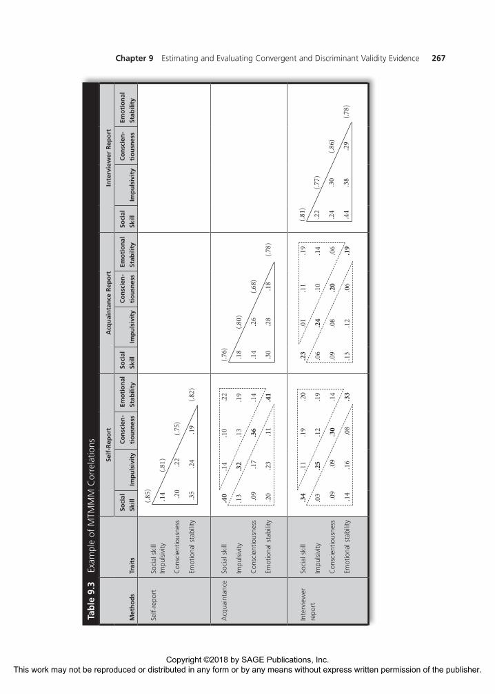
Campbell and Fiske (1959) articulated the definitions and logic of these four types of correlations, and they tied them to construct validity. A full MTMMM of hypothetical correlations is presented in Table 9.3. The matrix includes 66 correlations among the three measures of four traits, along with 12 reliability estimates along the main diagonal. Each of these 78 values can be characterized in terms of the four types of correlations just outlined. The evaluation of construct validity, trait variance, and method variance proceeds by focusing on various types of correlations as organized in the MTMMM.

Evidence of convergent validity is represented by monotrait–heteromethod cor-relations, which are printed in boldface in the MTMMM. Again, these are correla-tions between different ways of measuring the same traits. For example, the correlation between self-report social skill and acquaintance-report social skill is .40, and the correlation between self-report social skill and interviewer-report social skill is .34. These correlations suggest that people who describe themselves as relatively socially skilled (on the new self-report measure) tend to be described by their acquaintances and by the interviewers as relatively socially skilled. Such monotrait–heteromethod correlations that are fairly strong begin to provide good convergent evidence for the new self-report measure of social skill. However, they must be interpreted in the context of the other correlations in the MTMMM.

To provide strong evidence of its convergent and discriminant validity, the self-report measure of social skill should be more highly correlated with other measures of social skill than with any other measures. Illustrating this, the MTMMM in Table 9.3 shows that, as would be expected, the monotrait–heteromethod correla-tions are generally larger than the heterotrait–heteromethod correlations (inside the dashed-line triangles, reflecting the associations between measures of different constructs assessed through different methods). For example, the correlation between the self-report measure of social skill and the acquaintance-report mea-sure of emotional stability is only .20, and the correlation between the self-report measure of social skill and the interviewer-report measure of conscientiousness is only .09. These correlations, as well as most of the other heterotrait–heteromethod



Tab

le 9

.3

Exam

ple

of M

TMM

M C

orre

latio

ns

Met

ho

ds

Trai

ts

Self

-Rep

ort

Acq

uai

nta

nce

Rep

ort

Inte

rvie

wer

Rep

ort

Soci

al

Skill

Imp

uls

ivit

y

Co

nsc

ien

-

tio

usn

ess

Emo

tio

nal

Stab

ility

Soci

al

Skill

Imp

uls

ivit

y

Co

nsc

ien

-

tio

usn

ess

Emo

tio

nal

Stab

ility

Soci

al

Skill

Imp

uls

ivit

y

Co

nsc

ien

-

tio

usn

ess

Emo

tio

nal

Stab

ility

Self-

repo

rtSo

cial

ski

ll Im

puls

ivity

Con

scie

ntio

usne

ss

Emot

iona

l sta

bilit

y

Acq

uain

tanc

eSo

cial

ski

ll

Impu

lsiv

ity

Con

scie

ntio

usne

ss

Emot

iona

l sta

bilit

y

Inte

rvie

wer

repo

rtSo

cial

ski

ll

Impu

lsiv

ity

Con

scie

ntio

usne

ss

Emot

iona

l sta

bilit

y

(.85

)

.14

(.81

)

.20

.22

(.75

)

.35

.24

.19

(.82

)

.40

.14

.10

.22

.13

.32

.13

.19

.09

.17

.36

.14

.20

.23

.11

.41

.34

.11

.19

.20

.03

.25

.12

.19

.09

.09

.30

.14

.14

.16

.08

.33

(.76

)

.18

(.80

)

.14

.26

(.68

)

.30

.28

.18

(.78

)

.23

.01

.11

.19

.06

.24

.10

.14

.09

.08

.20

.06

.13

.12

.06

.19

(.81

)

.22

(.77

)

.24

.30

(.86

)

.44

.38

.29

(.78

)



correlations, are noticeably lower than the monotrait–heteromethod correlations discussed in the previous paragraph (which were larger correlations of .40 and .34). Thus, the correlations between measures that share trait variance but do not share method variance (the monotrait–heteromethod correlations) should be larger than the correlations between measures that share neither trait variance nor method variance (the heterotrait–heteromethod correlations).

An even more stringent requirement for convergent and discriminant validity evidence is that the self-report measure of social skill should be more highly cor-related with other measures of social skill than with self-report measures of other traits. The MTMMM in Table 9.3 shows that, as would be expected, the monotrait–heteromethod correlations are generally larger than the heterotrait–monomethod correlations (inside the solid-line triangles reflecting the associations between measures of different constructs assessed through the same method). The values in the MTMMM in Table 9.3 provide mixed evidence in terms of these associations. Although the correlations between the self-report measure of social skill and the self-report measures of impulsivity and conscientiousness are relatively low (only .14 and .20, respectively), the correlation between the self-report measure of social skill and the self-report measure of emotional stability is relatively high, at .35. Thus, the self-report measure of social skill overlaps with the self-report measure of emotional stability. Moreover, it overlaps with this measure of a different construct to the same degree that it overlaps with other measures of social skill. That is, self-reported social skill is correlated with self-reports of a different trait (i.e., emotional stability) to about the same degree that it is correlated with other ways of measuring the same trait (i.e., social skill). This is a potential problem, as it raises concerns about the discriminant validity of the self-report measure that is supposed to assess social skill. Thus, the correlation between measures that share trait variance but do not share method variance (the monotrait–heteromethod correlations) should be larger than the correlations between measures that do not share trait variance but do share method variance (the heterotrait–monomethod correlations). Ideally, the researchers would like to see even larger monotrait–heteromethod correlations than those in Table 9.3 and even smaller heterotrait–monomethod correlations.

In sum, an MTMMM analysis, as developed by Campbell and Fiske (1959), provides useful guidelines for evaluating construct validity. By carefully consider-ing the important effects of trait variance and method variance on correlations among measures, researchers can use the logic of an MTMMM analysis to gauge convergent and discriminant validity. In the decades since Campbell and Fiske published their highly influential work, researchers interested in measurement have developed even more sophisticated ways of statistically analyzing data obtained from an MTMMM study. For example, Widaman (1985) and others (Eid et al., 2008; Kenny, 1995) have developed strategies for using confirmatory factor analysis (see Chapter 12) to analyze MTMMM data. Although such procedures are beyond the scope of our discussion, readers should be aware that psychometricians con-tinue to build on the work by Campbell and Fiske.

Despite the strong logic and widespread awareness of the approach, the MTMMM approach to evaluating convergent and discriminant validity evi-dence does not seem to be used very frequently. For example, we conducted a



quick review of articles published in the last three issues of the 2016 volume of Psychological Assessment, which is a research journal published by the American Psychological Association (APA). The journal is intended to present “empirical research relevant to assessments conducted in the broad field of clinical psychology,” including research related to “development, validation, and appli-cation of assessment instruments, scales, observational methods, and inter-views” (APA, n.d.). In our review, we identified 13 articles claiming to present evidence related to convergent and discriminant validity or construct validity more generally. Of these 13 articles, only 2 mentioned an MTMMM approach. Furthermore, one of those two articles treated positively keyed versus negatively keyed items as the “multimethod” component of the analysis, with all assess-ments being based on self-reports. Although this review is admittedly limited and quite informal, it underscores our impressions of the (in)frequency with which MTMMM analyses are used.

Regardless of the frequency of its use, the MTMMM has been an important development in the understanding and analysis of convergent and discriminant validity evidence. It has shaped the way many people think about construct validity, and it is an important component of a full understanding of psychometrics.

Quantifying Construct Validity

The final method that we will discuss for evaluating convergent and discriminant validity evidence is a more recent development. Westen and Rosenthal (2003) out-lined a procedure that they called “quantifying construct validity” (QCV), in which researchers formally quantify the degree of “fit” between (a) their theoretical pre-dictions for a set of convergent and discriminant correlations and (b) the set of correlations that are actually obtained.

At one level, this should sound familiar, if not redundant! Indeed, an overriding theme in our discussion of construct validity is that the theoretical basis of a con-struct guides the study and interpretation of validity evidence. For example, in the previous sections, we have discussed various ways in which researchers identify the criterion variables used to evaluate convergent and discriminant validity evidence, and we have emphasized the importance of interpreting validity correlations in terms of conceptual relevance to the construct of interest.

However, in practice, evidence regarding convergent and discriminant validity often rests on rather subjective and impressionistic interpretations of validity cor-relations. For example, in our earlier discussion of the “sets of correlations” approach to convergent and discriminant validity evidence, we stated that researchers often “eyeball” the correlations and make a somewhat subjective judgment about the degree to which the correlations match their expectations (as based on the nomo-logical network surrounding the construct of interest). We also stated that research-ers often judge the degree to which the pattern of convergent and discriminant correlations “makes sense” in terms of the theoretical basis of the construct being assessed by a test. But what if one researcher’s judgment of what makes sense does not agree with another’s judgment? And exactly how strongly do the convergent and discriminant correlations actually fit with the theoretical basis of the construct?



Similarly, when examining the MTMMM correlations, we stated that some cor-relations were “generally larger” or “noticeably lower” than others. We must admit that we tried to sneak by without defining what we meant by “generally larger” and without discussing exactly how much lower a correlation should be to be considered “noticeably” lower than another. In sum, although the correlations themselves are precise estimates of association, the interpretation of the overall pattern of conver-gent and discriminant correlations often has been done in a somewhat imprecise and subjective manner.

Given the common tendency to rely on somewhat imprecise and subjective evaluations of patterns of convergent and discriminant correlations, the QCV pro-cedure was designed to provide a more precise and more objective quantitative estimate of the support provided by the overall pattern of evidence. Thus, the emphasis on precision and objectivity is an important difference from the previous strategies. The QCV procedure is intended to provide an answer to a single ques-tion in an examination of the validity of a measure’s interpretation: “Does this measure predict an array of other measures in a way predicted by theory?” (Westen & Rosenthal, 2003, p. 609).

There are two complementary kinds of results obtained in a QCV analysis. First, researchers obtain two effect sizes representing the degree of fit between the actual pattern of correlations and the predicted pattern of correlations. These effect sizes, called ralerting-CV and rcontrast-CV, are correlations themselves, ranging between −1 and +1. We will discuss the nature of these effect sizes in more detail, but for both, large positive effect sizes indicate that the actual pattern of convergent and discriminant correlations closely matches the pattern of correlations predicted on the basis of the conceptual meaning of the constructs being assessed. The second kind of result obtained in a QCV analysis is a test of statistical significance. The significance test indicates whether the degree of fit between actual and predicted correlations is likely to have occurred by chance. Researchers conducting a validity study using the QCV procedure will hope to obtain large values for the two effect sizes, along with statistically significant results.

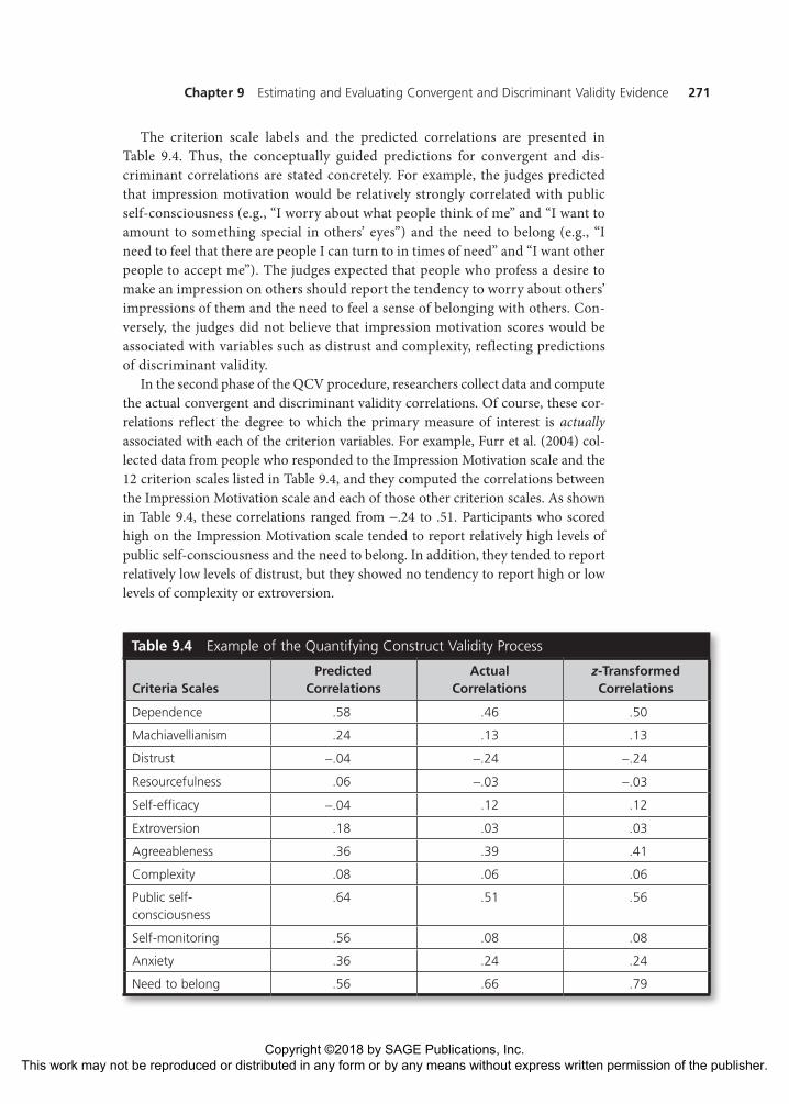
The QCV procedure can be summarized in three phases. First, researchers must generate clear predictions about the pattern of convergent and discriminant validity correlations that they would expect to find. They must think carefully about the criterion measures included in the study, and they must form predictions for each one, in terms of its correlation with the primary measure of interest. For example, Furr and his colleagues (Furr, Reimer, & Bellis, 2004; Nave & Furr, 2006) developed a measure of impression motivation, which was defined as a person’s general desire to make specific impressions on other people. To evaluate the convergent and dis-criminant validity of the scale, participants were asked to complete the Impression Motivation scale along with 12 additional “criterion” personality questionnaires. To use the QCV procedure, Furr et al. (2004) needed to generate predictions about the correlations that would be obtained between the Impression Motivation scale and the 12 criterion scales. They did this by recruiting five professors of psychology to act as “expert judges.” The judges read descriptions of each scale, and each one provided predictions about the correlations. The five sets of predictions were then averaged to generate a single set of predicted correlations.



The criterion scale labels and the predicted correlations are presented in Table 9.4. Thus, the conceptually guided predictions for convergent and dis-criminant correlations are stated concretely. For example, the judges predicted that impression motivation would be relatively strongly correlated with public self-consciousness (e.g., “I worry about what people think of me” and “I want to amount to something special in others’ eyes”) and the need to belong (e.g., “I need to feel that there are people I can turn to in times of need” and “I want other people to accept me”). The judges expected that people who profess a desire to make an impression on others should report the tendency to worry about others’ impressions of them and the need to feel a sense of belonging with others. Con-versely, the judges did not believe that impression motivation scores would be associated with variables such as distrust and complexity, reflecting predictions of discriminant validity.

In the second phase of the QCV procedure, researchers collect data and compute the actual convergent and discriminant validity correlations. Of course, these cor-relations reflect the degree to which the primary measure of interest is actually associated with each of the criterion variables. For example, Furr et al. (2004) col-lected data from people who responded to the Impression Motivation scale and the 12 criterion scales listed in Table 9.4, and they computed the correlations between the Impression Motivation scale and each of those other criterion scales. As shown in Table 9.4, these correlations ranged from −.24 to .51. Participants who scored high on the Impression Motivation scale tended to report relatively high levels of public self-consciousness and the need to belong. In addition, they tended to report relatively low levels of distrust, but they showed no tendency to report high or low levels of complexity or extroversion.

Table 9.4 Example of the Quantifying Construct Validity Process

Criteria ScalesPredicted

CorrelationsActual

Correlationsz-Transformed Correlations

Dependence .58 .46 .50

Machiavellianism .24 .13 .13

Distrust −.04 −.24 −.24

Resourcefulness .06 −.03 −.03

Self-efficacy −.04 .12 .12

Extroversion .18 .03 .03

Agreeableness .36 .39 .41

Complexity .08 .06 .06

Public self-consciousness

.64 .51 .56

Self-monitoring .56 .08 .08

Anxiety .36 .24 .24

Need to belong .56 .66 .79



In the third phase, researchers quantify the degree to which the actual pattern of convergent and discriminant correlations fits the predicted pattern of correlations. A close fit provides good evidence of validity for the intended interpretation of the test being evaluated, but a weak fit would imply poor validity. As described earlier, the fit is quantified by two kinds of results—effect sizes and a significance test.

The two effect sizes reflect the amount of evidence of convergent and discrimi-nant validity as a matter of degree. The ralerting-CV effect size is (more or less) the correlation between the set of predicted correlations and the set of actual correla-tions. A large value would indicate that the correlations that the judges predicted to be relatively large were indeed the ones that actually were relatively large, and it indicates that the correlations that the judges predicted to be relatively small were indeed the ones that actually were relatively small.

Take a moment to examine the correlations in Table 9.4. Note, for example, that the judges predicted that dependence, public self-consciousness, self-monitoring, and the need to belong would have the largest correlations with social motivation. In fact, three of these four scales did have the largest correlations. Similarly, the judges predicted that distrust, resourcefulness, self-efficacy, and complexity would have the weakest correlations with social motivation. Indeed, three of these four scales did have the weakest correlations (relative to the others). Thus, the pattern of actual cor-relations generally matched the predictions made by the judges. Consequently, the ralerting-CV value for the data in Table 9.4 is .79, a large positive correlation. In actuality, the ralerting-CV value is computed as the correlation between the predicted set of cor-relations and the set of “z-transformed” actual correlations. The z transformation is done for technical reasons regarding the distribution of the underlying correlation coefficients. For all practical purposes, though, the ralerting-CV effect size simply repre-sents the degree to which the correlations that are predicted to be relatively high (or low) are the correlations that actually turn out to be relatively high (or low).

Although its computation is more complex, the rcontrast-CV effect size is similar to the ralerting-CV effect size in that large positive values indicate greater evidence of con-vergent and discriminant validity. Specifically, the computation of rcontrast-CV adjusts for the intercorrelations among the criterion variables and for the absolute level of correlations between the main test and the criterion variables. For the data collected by Furr et al. (2004), the rcontrast-CV value was approximately .68, again indicating a high degree of convergent and discriminant validity. As the QCV procedure is a relatively recent development—at least as compared with the other procedures we have discussed—there are no clear guidelines about how large the effect sizes should be to be interpreted as providing evidence of adequate validity. At this point, we can say simply that higher effect sizes offer greater evidence of validity.

In addition to the two effect sizes, the QCV procedure provides a test of statisti-cal significance. Based on a number of factors, including the size of the sample and the amount of support for convergent and discriminant validity, a z test of signifi-cance indicates whether the results are likely to have been obtained by chance.

Although the QCV approach is a potentially useful approach to estimating con-vergent and discriminant evidence, it is not perfect. For example, low effect sizes (i.e., low values for ralerting-CV and rcontrast-CV) might not necessarily indicate poor evi-dence of validity. Low effect sizes could result from an inappropriate set of



predicted correlations. If the predicted correlations are poor reflections of the nomological network surrounding a construct, then a good measure of the con-struct will produce actual correlations that do not match the predictions. Similarly, a poor choice of criterion variables could result in low effect sizes. If few of the criterion variables used in the validity study are associated with the main test of interest, then they do not represent the nomological network well. Thus, the crite-rion variables selected for a QCV analysis should represent a range of strong and weak associations, reflecting a clear pattern of convergent and discriminant evi-dence. Indeed, Westen and Rosenthal (2005) point out that “one of the most impor-tant limitations of all fit indices is that they cannot address whether the choice of items, indicators, observers, and so forth was adequate to the task” (p. 410).

In addition, the QCV procedure has been criticized for resulting in “high correlations in cases where there is little agreement between predictions and observations” (G. T. Smith, 2005, p. 404). That is, researchers might obtain apparently large values for ralerting-CV and even rcontrast-CV when the observed pat-tern of convergent and discriminant validity correlations does not match closely the actual pattern of convergent and discriminant validity correlations. Westen and Rosenthal (2005) acknowledge that this might be true in some cases; however, they suggest that the QCV procedures are “aids to understand-ing” and should be carefully scrutinized in the context of many conceptual, methodological, and statistical factors (p. 411).

Finally, the statistical values produced by the QCV procedure (e.g., ralerting-CV , z test of significance, etc.) require complex computations, and until recently, no statistical packages provided easy ways to conduct those computations. Fortunately, a user-friendly function in R is now available, allowing researchers to obtain QCV statistical results relatively easily (Heuckeroth & Furr, 2017).

In this section, we have outlined several strategies that can be useful in many areas of test evaluation; however, there is no single perfect method or statistic for estimating the overall convergent and discriminant validity of test interpretations. Although it is not perfect, the QCV does offer several advantages over some other strategies. First, it forces researchers to consider carefully the pattern of convergent and discriminant associations that would make theoretical sense, on the basis of the construct in question. Second, it forces researchers to make explicit predictions about the pattern of associations. Third, it retains the focus on the measure of pri-mary interest. Fourth, it provides a single interpretable value reflecting the overall degree to which the pattern of predicted associations matches the pattern of associa-tions that is actually obtained, and finally, it provides a test of statistical significance. Used with care, the QCV is an important addition to the toolbox of validation.

Factors Affecting a Validity Coefficient

The strategies outlined above are used to accumulate and interpret evidence of convergent and discriminant validity. To some extent, all of the strategies rest on the size of validity coefficients—statistical results that represent the degree of



association between a test of interest and one or more criterion variables. In this section, we address some important factors that affect validity coefficients.

When conducting or reading studies regarding validity, it is important to be aware of these factors. For a truly informed understanding of validity research, it is important to understand why a test’s scores might be strongly or, more problematic, weakly associated with key criterion variables. Indeed, there are many reasons why a test’s scores might not be strongly associated with key criterion variables. Although weak convergent associations might reflect flaws in the test, we shall see that such results might not actually reflect shortcomings in the test itself. By considering the various factors that can affect these associations, people who produce and interpret validity studies will reach conclusions that are more well informed and accurate.

Thus far, we have emphasized the correlation as a coefficient of validity because of its interpretability as a standardized measure of association. Although other sta-tistical values can be used to represent associations between tests and criterion variables (e.g., regression coefficients), most such values are built on correlation coefficients. Thus, our discussion centers on some of the key psychological, meth-odological, psychometric, and statistical factors affecting correlations between tests and criterion variables.

Associations Between Constructs

One factor affecting the correlation between measures of two constructs is the “true” association between those constructs. If two constructs are strongly associated with each other, then measures of those constructs will likely be highly correlated with each other. Conversely, if two constructs are unrelated to each other, then measures of those constructs will probably be weakly correlated with each other. Indeed, when we conduct research in general, we intend to interpret the observed associations that we obtain (e.g., the correlations between the measured variables in our study) as approximations of the true associations between the constructs in which we are interested. When we conduct validity research, we predict that two measures will be correlated because we believe that the two constructs are associated with each other.

Random Measurement Error and Reliability

In earlier chapters (Chapters 5–7), you learned about the conceptual basis, the esti-mation, and the importance of reliability as an index of (the lack of) random mea-surement error. As we discussed in those chapters, one important implication of random measurement error is its effect on correlations between tests—it reduces, or attenuates, the correlation between tests. Therefore, random measurement error affects validity coefficients, just like any other correlation.

As we saw in earlier chapters, the correlation between tests (say X and Y) of two constructs is a function of the true correlation between the two constructs and the reliabilities of the two tests (if key assumptions of classical test theory hold true):

r r R R .X Y X Y XX YYo o t t= (9.1)



In this equation, r r R R .X Y X Y XX YYo o t t= is the correlation between the two tests (i.e., the correlation

between the observed scores). More specifically, it is the validity correlation between the primary test of interest (say the “X” test) and the test of a criterion variable (the “Y” test). In addition, r r R R .X Y X Y XX YYo o t t

= is the true correlation between the two constructs, RXX is the reliability of the test of interest, and RYY is the reliability of the test of the criterion variable.

For example, in their examination of the convergent validity evidence for their measure of impression motivation, Furr et al. (2004; Nave & Furr, 2006) were inter-ested in the correlation between impression motivation and public self- consciousness. Imagine that the true correlation between the constructs is .60. What would the actual validity correlation be if the two tests had poor reliability? If the impression motivation test had a reliability of .63 and the public self-consciousness test had a reliability of .58, then the actual validity coefficient obtained would be only .36:

r .60 .63 .58,

.60 .604 ,

.36.

X Yo o

( )=

==

Recall that to evaluate convergent validity, researchers should compare their correlations with the correlations that they would expect based on the constructs being measured. In this case, if Furr et al. (2004) were expecting to find a correlation close to .60, then they might be relatively disappointed with a validity coefficient of “only” .36. Therefore, they might conclude that their test has poor validity as a measure of impression motivation.

Note that the validity coefficient is affected by two reliabilities: (1) the reliability of the test of interest and (2) the reliability of the criterion test. Thus, the primary test of interest could be a good measure of the intended construct, but the validity coefficient could appear to be poor. For example, if the impression motivation test had a good reliability of, say, .84 but the public self-consciousness test had a very poor reliability of .40, then the actual validity coefficient obtained would be only .35:

r .60 .84 .40,

.60 .580 ,

.35.

X Yo o

( )=

==

So even if the primary test is psychometrically strong and interpreted validly, the use of a psychometrically weak criterion measure will produce poor validity coefficients.

Therefore, when evaluating the size of a validity correlation, it is important to consider both the reliability of the primary test of interest and the reliability of the criterion test. If either one or both is relatively weak, then the resulting validity cor-relation is likely to appear relatively weak. This might be a particularly subtle con-sideration for the criterion variable. Even if the primary test of interest is a good measure of its intended construct, we might find poor validity correlations. That is, if the criterion measures that we use are poor, then we are unlikely to find evidence supporting the validity of the primary test! This important issue is easy to forget.



There are rough guidelines for identifying problematic levels of reliability and for handling those problems. As mentioned in Chapter 5, researchers are generally satisfied if a test’s reliability is above .70 or .80, with higher levels being even better. If a test’s or a criterion variable’s reliability is much lower than this, then we would have concerns about its effect on validity coefficients. Of course, the lower one or more of the reliabilities are, the greater our concern would be.

In terms of handling the problem, there are at least two possibilities. One is to simply discount a validity coefficient that is based on poor reliability, or at least to reduce the weight that one would give it in one’s consideration of validity evidence.

The other possibility is to use the logic of the correction for attenuation dis-cussed in Chapter 7 to adjust the validity coefficient. However, it might make sense to adjust only for the criterion variable’s reliability. That is, if the purpose of a vali-dation analysis is to evaluate the psychometric quality of a particular test, then it seems inadvisable to adjust for that test’s lack of psychometric quality. Thus, to adjust for only one test’s reliability, researchers can use the following variation on the correction for attenuation:

=r

rR

,XYXY

YY-adjusted

-original

(9.2)

where rXY-original is the original validity correlation, RYY is the estimated reliability of the criterion variable (i.e., not the test of interest being validated), and rXY-adjusted is the adjusted validity correlation. This equation adjusts a validity correlation by assuming that the criterion variable is measured without any measurement error.

Restricted Range

Recall from Chapter 3 that a correlation coefficient reflects covariability between two distributions of scores. That is, it represents the degree to which variability in one distribution of scores (e.g., scores on a test to be validated) corresponds with variability in another distribution of scores (e.g., scores on a test of a criterion variable). From this perspective, it is important to realize that the amount of vari-ability in one or both distributions of scores can affect the correlation between the two sets of scores. Specifically, a correlation between two variables can be reduced if the range of scores in one or both variables is artificially limited or restricted.

A classic example of this is the association between SAT scores and academic performance. Earlier, we discussed the fact that much of the evidence for the quality of the SAT scores rests on the correlation between SAT scores and academic perfor-mance as measured by college grade point average (GPA). Indeed, a college might wish to evaluate the validity of the SAT as a predictor of GPA among its students. That is, the college examines whether students who score relatively high on the SAT tend to have relatively good performance at the college. Implicitly, this demonstra-tion requires that people who score relatively low on the SAT tend to have relatively poor performance in college. To demonstrate this kind of association, the college would need to demonstrate that variability in the distribution of SAT scores corre-sponds with variability in the distribution of college GPAs. However, the ability to demonstrate this association is minimized by restricted range in two ways.



First, range restriction exists in GPA as a measure of academic performance. In most colleges, GPA can range only between 0.0 and 4.0. The worst that any student can do is a GPA of 0.0, and the best that any student can do is 4.0. But does this 4-point range in GPA really reflect the full range of possible academic performance? Consider two students, Leo and Mary, who do well in classes and earn As in all of their courses. Although Leo did perform well, he barely earned an A in each of his courses. So he “squeaked by” with a 4.0, and the 4.0 in a sense represents the upper limit of his academic performance. Mary also performs well, earning As in all of her courses. But Mary outperformed every other student in each of her courses. In each course, she was the only one to earn an A on any test, and she had clearly mastered all the material on each and every assignment that her professors graded. So Mary also received a 4.0, but her 4.0 in a sense underestimates her academic ability. She had mastered all the material so well that her professors wished that they could give her grades higher than an A. Although Leo and Mary received the same “score” on the measure of academic performance (i.e., they both have 4.0 GPAs), they actually differ in the quality of their performance. Leo fully earned his 4.0 and should be proud of it, but the professors would probably agree that Mary outperformed him. Thus, the 4-point GPA scale restricts the range of measurement of academic performance.

Note that GPA is restricted in both directions—on the high end and on the low end. Consider Jenny and Bruce. Although both Jenny and Bruce failed all of their classes, Bruce nearly passed each class. On the other hand, Jenny wasn’t even close to passing any classes. So both Bruce and Jenny earned a GPA of 0.0, but in a sense, Bruce had better academic performance than Jenny. In terms of test grades, home-work grades, and paper grades, Bruce outperformed Jenny (i.e., he received 59 on each assignment, while she received scores in the 30s on each assignment). Despite the difference in their performance during the semester, Jenny could not receive a lower GPA than Bruce, because the GPA scale “bottoms out” at 0.0.

The scatterplot in Figure 9.1a shows a hypothetical data set for 5,000 students at a college that might be interested in evaluating the validity of the SAT as a predictor of academic performance. This scatterplot presents the idealized asso-ciation between SAT scores and “unrestricted” college GPA. That is, it presents scores for students whose academic performance is not restricted by a 4-point GPA scale. Notice that some unrestricted GPA scores fall below 0.0 on the plot, reflecting differences between students like Jenny and Bruce. Notice also that some GPA scores fall above 4.0, reflecting differences between students like Leo and Mary.

For the data displayed in Figure 9.1a, the correlation between SAT and GPA was .605. This indicates that students who received relatively low SAT scores tended to have relatively low “unrestricted” GPAs (and, obviously, students who received rela-tively high SAT scores tended to have relatively high “unrestricted” GPAs).

But of course, GPA actually is restricted, as just discussed. Therefore, students whose academic performance might, theoretically, merit a 5.0 or a 6.0 can earn only a 4.0 in practice. Similarly, students whose academic performance might merit a GPA below 0 cannot actually receive less than 0. So all those students who might, in an abstract sense, deserve GPAs above 4.0 (or below 0) will in reality receive a GPA of 4.0 (or 0).



With this in mind, the scatterplot in Figure 9.1b shows the data for the same 5,000 students, based on the “restricted” GPA scores. Note that there are now no GPA scores above 4.0—the scores are “maxed out” at 4.0. Similarly, there are no GPA scores below 0.0—the scores are bottomed out at 0. This scatterplot appears to be more compressed, and the association between SAT and GPA might not seem as clear as it was in the first scatterplot (Figure 9.1a). Consequently, for the data displayed in Figure 9.1b, the cor-relation between SAT and GPA was reduced, a bit, to .603. Thus, the restriction of range in GPA scores has a very slight diminishing effect on the correlation.

Figure 9.1 Scatterplots Illustrating Range Restriction

400 600 800 1000 1200 1400 1600

9.1a − Plot of Unrestricted SAT and Unrestricted GPA

Correlation = 0.605

−2

0

2

4

6

SAT

GPA

400 600 800 1000 1200 1400 1600

9.1b − Plot of Unrestricted SAT and Restricted GPA

Correlation = 0.603

−2

0

2

4

6

SAT

GPA

400 600 800 1000 1200 1400 1600

9.1c − Plot of Restricted SAT and Restricted GPA

Correlation = 0.474

−2

0

2

4

6

SAT

GPA



A second way in which range restriction minimizes the ability to demonstrate the association between SAT scores and academic performance is in the number of people who actually obtain college GPAs. That is, students with very low SAT scores are much less likely to be admitted to college than are students with higher SAT scores. If a college truly was to conduct a real study of the association between SAT scores and academic performance, it would probably be limited to a subsample of all the students who have SAT scores. This is because it would be limited to only those students who took the SAT and who were admitted to the college. For better or for worse, not all students who take the SAT are admitted to college. For exam-ple, it is quite possible that highly competitive colleges might be reluctant to admit students who have SAT scores below, say, 900. In our hypothetical data set of 5,000 students, nearly 1,400 had SAT scores below 900. In reality, these people might not be admitted to the competitive college conducting the study; therefore, they would never actually have a college GPA score.

With this in mind, the scatterplot in Figure 9.1c shows the data for the remaining 3,605 students with SAT scores greater than 900. Note that there are no people with SAT scores below 900. That is, for a stark illustration of range restriction, we are assuming that none of those people would be admit-ted to the competitive college, and thus they would not be included in an analysis of the association between SAT scores and college GPAs. Obviously, this scatterplot is even more compressed than the previous two. Consequently, for the data displayed in Figure 9.1c, the correlation between SAT and GPA was reduced even more, to .474.

Unfortunately, there are no clear, simple guidelines about detecting range restriction; rather, it requires careful thought and attention from researchers. For example, it would require knowledge about the relevant tests or variables (e.g., knowing that GPA scores range from 0 to 4 and that SAT scores range from 400 to 1,600). In addition, it would require examination of the scores obtained in a given study in comparison with the range of possible scores on the relevant tests. For example, it would require a researcher to examine the actual range of SAT scores in a given analysis and to compare this range with the possible range of 400 to 1,600. If the range of obtained scores differs dramatically from the range of possible scores, then there might be reason for concern about range restriction. Perhaps more subtly, if the range of obtained scores falls within a certain “side” of the distribution of possible scores, then there might be particularly serious con-cerns about range restrictions. For example, the SAT scores in our analysis were mainly weighted toward the high end of possible SAT scores, with none in the range of 400 to 900.

Although there are no easy tricks to detect range restriction, there are proce-dures for adjusting or correcting correlations to account for range restriction (Hunter, Schmidt, & Le, 2006; Sackett & Yang, 2000; Schmidt, Oh, & Le, 2006; R. L. Thorndike, 1949). A full discussion of the wide variety of cases and procedures is beyond the scope of this section, but we will describe the most common correc-tion (Case 2 from R. L. Thorndike, 1949). This correction is designed for situations in which one variable (out of the two being correlated with each other) suffers from range restriction.



Imagine again the college that was interested in examining the predictive valid-ity of the SAT, and recall the finding that the correlation between restricted SAT scores and GPA was .474. Let’s say that they had concerns about range restriction in SAT scores and wished to obtain a corrected correlation.

To compute the corrected correlation, they would need just three values:

1. The first is the correlation they actually obtained (rrestricted), which in their study was rrestricted = .474. This is the correlation based on “restricted” SAT scores, and this is what they’d like to correct for range restriction in the SAT scores.

2. The second value is simply the standard deviation of the “restricted” SAT scores in their sample (srestricted). For the 3,605 SAT scores in Figure 9.1c, this value is srestricted = 129.55. Recall (Chapter 3) that a standard deviation reflects the amount of variability among a set of scores. Presumably, the range of SAT scores among the 3,605 students in the sample is meaningfully less than it would be if SAT scores were not cut off at 900.

3. Thus, the third value is the “unrestricted” standard deviation of SAT scores—the standard deviation that would be obtained across a fuller range of SAT scores (sunrestricted). This is a value that might need to be guessed, as researchers might not have data for calculating it. In the case of our hypothetical college, perhaps the college could calculate the standard deviation of all the SAT scores it receives during the admissions process—scores from applicants who were not admitted, in addition to scores from those who were. Alternatively, perhaps other published sources provide standard deviations for wide-ranging samples. If so, then the college might simply use those values. For the current case, let’s assume that the college does indeed calculate the standard deviation across the entire 5,000 applicants that it received. For the 5,000 scores in Figure 9.1b, this value is sunrestricted = 181.63. As anticipated, this value is noticeably larger than the restricted standard deviation (srestricted = 129.55), underscoring the idea that the sample’s range of SAT scores is indeed substantially narrower than a fuller range of scores.

Using these three statistical values, the college can compute a correlation that corrects for range restriction (runrestricted):

=

+ −

rr s

s

r ss

1 1

.unrestricted

restrictedunrestricted

restricted

restricted2 unrestricted

2

restricted2

(9.3)

In our hypothetical college’s case

=

+ −

r.474 181.63

129.55

1 .474 181.63129.55

1unrestricted

22

2

.



( )( )

=+ −

r.474 1.402

1 .225 1.965 1unrestricted .

=

+r .664

1 .217unrestricted .

=r .664

1.103unrestricted .

=r .602unrestricted .

Note that this is indeed very similar (within rounding error) to the correlation in Figure 9.1b. Again, this example outlines the procedure for a situation in which researchers wish to correct a correlation for range restriction in one variable. However, other situations might arise (e.g., correcting for range restriction in both variables). Interested readers can find useful information in a variety of sources (e.g., Hunter et al., 2006; Sackett & Yang, 2000).

In sum, our SAT and GPA example illustrates range restriction and its effect on validity correlations. Specifically, range restriction can shrink validity correla-tions, thereby appearing to provide relatively poor evidence of validity. When evaluating the quality of a psychological measure, we often depend on correlations (or other statistical values that are based on correlations) to reflect the degree of convergent and discriminant validity. And as we’ve discussed, when searching for convergent evidence, we expect to find strong correlations. However, we need to be aware that restricted range can reduce the correlations that are actually obtained in a validity study. In the current example, the correlation between SAT and GPA was affected by restriction in two ways, and it was somewhat smaller than an “unrestricted” correlation between SAT scores and academic perfor-mance. Test users and test developers should be aware of the way that range restriction can affect validity correlations, and they might choose to “correct” validity correlations for these effects.

Skew and Relative Proportions

Another factor that affects the size of a validity coefficient is the “skew” of the dis-tributions of scores being examined. In Chapter 3, we mentioned that some distri-butions of scores might be “normal” or symmetric, having just as many high scores as low scores. However, other distributions might be skewed, with an imbalance of high scores relative to low scores (see Figures 3.1 and 3.2).

Although this factor might not be as widely known as some of the other factors affecting validity coefficients, the skew of a variable can have a robust impact on correlations (Dunlap, Burke, & Greer, 1995). Specifically, if the two variables being correlated have different “skews,” then the correlation between those variables will be reduced. For example, imagine a case in which one variable is normally



distributed (i.e., unskewed; see Figure 3.1) but the other is heavily skewed in some way (e.g., Figure 3.2a). In this case, the correlation between those two variables can-not be 1.0; indeed, it might be capped at some relatively small value. In contrast, imagine that neither variable is skewed and that both are normally distributed. In this case, the correlation between the two variables can reach 1.0, and all else being equal, it will be larger than the correlation in the first case (where one variable was skewed). Thus, if a validation study is conducted on a variable that is heavily skewed, then we might obtain a relatively small validity coefficient.

For a demonstration and discussion of this effect, it might be most straightfor-ward to consider the association between a continuous variable and a dichotomous variable. Imagine that we developed a self-report inventory to measure depression. And imagine that we would like to evaluate its convergent quality by correlating its scores with diagnoses made by trained clinical psychologists. To do this, we recruit a sample of participants who complete our inventory and who are interviewed by clinicians. The clinicians then provide a diagnosis for each participant, labeling each participant as either depressed or nondepressed. Thus, our main test of inter-est (i.e., the new self-report inventory) is on a continuous scale, whereas the crite-rion variable (i.e., diagnosis) is a dichotomous categorical variable representing two groups of participants—those diagnosed with depression and those without depres-sion. To evaluate the validity of our new scale as a measure of depression, we might compute a validity correlation between these two variables.1 Indeed, we would hope to find that participants’ scores on our new inventory are strongly correlated with clinicians’ ratings.

In this case, the relative proportion of participants in the two groups is akin to the skew of the diagnosis variable. That is, if the groups are equally sized, then the diagnosis variable is unskewed; however, if the groups are not equally sized, then the diagnosis variable is skewed in some way. For example, if only a small propor-tion of participants are diagnosed as depressed, then the diagnosis variable will be heavily skewed in a way that is somewhat similar to the scatterplot in Figure 3.2a.

Thus, as implied earlier, the validity correlation between the two variables would be affected by the relative proportion of participants in each of the two diagnosis groups. More precisely, the size of the validity correlation between inventory scores and clinicians’ diagnoses is influenced by the proportion of participants who are diagnosed as having depression (vs. not having depression). If the group sizes are equal, then the validity correlation is likely to be larger than when the group sizes are unequal (McGrath & Meyer, 2006). Following from this, if our validation study is conducted on groups having heavily unequal numbers of participants, then we might obtain a relatively small validity coefficient.

Let us examine and demonstrate this influence concretely. If we were computing the validity correlation in this example, each participant would have scores on two variables—depression inventory score and diagnostic category—as illustrated by the hypothetical data in Table 9.5. Obviously, the depression inventory scores are already on a quantitative scale (let us say that scores can range from 0 to 30). How-ever, the diagnostic category variable must be quantified so that we can compute the validity correlation. To do this, we assign one value to all participants diagnosed as nondepressed and another value to all participants diagnosed as depressed.



These values could be 1 and 2, 1 and 10, −1,000 and +1,000, or any other pair of numbers (as long as all the people in each group receive the same value). For our purposes, we will code the “nondepressed” group as “1” and the depressed group as “2” (see Table 9.5).

Recall from Chapter 3 that the correlation between two variables is the covari-ance between the two variables divided by the product of their two standard devia-tions (see Equation 3.5). For a correlation between one continuous variable (C ) and one dichotomous variable (D), the correlation (rCD) is

=r

cs s

,CDCD

C D (9.4)

Table 9.5 Data Illustrating the Effect of Relative Proportions on Validity Coefficients

ParticipantDepression Inventory Diagnosis Diagnosis Code

1 6 Nondepressed 1

2 5 Nondepressed 1

3 7 Nondepressed 1

4 1 Nondepressed 1

5 11 Nondepressed 1

6 9 Nondepressed 1

7 3 Nondepressed 1

8 6 Nondepressed 1

9 4 Nondepressed 1

10 8 Nondepressed 1

11 10 Nondepressed 1

12 2 Nondepressed 1

13 5 Nondepressed 1

14 7 Nondepressed 1

15 6 Nondepressed 1

16 10 Depressed 2

17 15 Depressed 2

18 5 Depressed 2

19 8 Depressed 2

20 12 Depressed 2

Mean 7.00 .25

Standard deviation 3.39 .43

Covariance .75

Correlation .51



where cCD is the covariance between the two variables, sC is the standard deviation of the continuous variable, and sD is the standard deviation of the dichotomous variable.

Two of these terms are directly affected by the proportion of observations in the two groups, as defined by the dichotomous variable. Assuming that the groups are coded “1” (for Group 1) and “2” (for Group 2), then the covariance is

= −c p p C C( ),CD 1 2 2 1 (9.5)

where p1 and p2 are the proportion of participants in Groups 1 and 2, respectively; = −c p p C C( ),CD 1 2 2 1 is the mean of the continuous variable for the participants in Group 1; and = −c p p C C( ),CD 1 2 2 1

is the mean of the continuous variable for the participants in Group 2. In our data set, 15 of the 20 participants are in the nondepressed diagnostic group (Group 1), and 5 are in the depressed group (Group 2). Thus, the two proportions are .75 (15/20 = .75) and .25 (5/20 = .25). In addition, the average score on the depres-sion inventory is 6 for the nondepressed group and 10 for the depressed group. Thus, the covariance is

cCD = (.75)(.25)(10 − 6),

= (.1875)(4),

= .75.

The standard deviation of the dichotomous variable is the second term affected by the proportion of observations in the two groups defined by the dichotomous variable. Again, assuming that the groups are coded “1” (for Group 1) and “2” (for Group 2), then based on our discussion of binary (i.e., dichotomous) items in Chapter 3 and Equation 3.9, we know that this standard deviation is

=s p p .D 1 2 (9.6)

For the data in Table 9.5, the standard deviation of the dichotomous “diagnosis” variable is

=

=

s (.75)(.25),

.433.

D

Taking these terms into account, the equation for the correlation can be reframed and simplified to show the direct influence of the relative proportions:

= −

=−

r p p C Cs p p

rp p C C

s

( ) ,

( ).

CDc

CDC

1 2 2 1

1 2

1 2 2 1

(9.7)

For the example data in Table 9.5, the validity correlation is



= −

=

=

r (.75)(.25)(10 6)3.39

,

1.723.39

,

.51.

CD

This correlation is positive and fairly strong, indicating good convergence between our new scale and clinicians’ diagnoses. More specifically, it reveals that those participants who had relatively “high scores” on the diagnosis variable also tended to have higher scores on the depression inventory than did those participants who had relatively “low scores” on the diagnosis variable. It might seem odd to think of “high scores” or “low scores” on a diagnosis, but recall the way we coded the diagnoses (Table 9.5). That is, we coded the diagnosis variable so that the participants who were diagnosed as depressed had “higher” diagnosis scores (i.e., a score of 2) than the participants who were diagnosed as nondepressed (who were given a score of 1). Therefore, we can interpret the correlation as showing that the participants diagnosed as depressed (i.e., those with relatively high scores on the diagnosis variable) tended to obtain high scores on the depression inventory as compared with the participants diagnosed as nondepressed (i.e., those with relatively low scores on the diagnosis variable). Again, this pattern of findings would provide some evidence of the validity of our new inventory as a measure of depression. However, it is worth considering how skew (i.e., differential group size in the current example) is affecting this validity correlation.

Equation 9.6 reveals the influence of group proportions on validity correlations. All else being equal, equally sized groups will allow larger correlations than will unequal groups. If two groups are equally sized, then the two proportions are .5 and .5. The product of these two proportions (.5 × .5 = .25) is the maximum of any two proportions. That is, any other pair of proportions will produce a product less than .25, and the greater the disparity in group sizes, the lower the product (e.g., .40 × .60 = .24, .10 × .90 = .09). And as shown in Equation 9.7, all else being equal, lower products will produce lower correlations.

For example, consider the validity correlation that we’d obtain if the two group sizes were even more discrepant than .75 versus .25. Let’s imagine that instead the depressed group was only 10% of the sample, but that all other values were the same (i.e., the same group means on the depression inventory and the same standard deviation on the inventory):

= −

=

=

r (.90)(.10)(10 6)3.39

,

1.203.39

,

.35.

CD

In this case, the validity correlation would be reduced noticeably, as compared with the case in which the groups were closer to being evenly sized. Depending on



the specific magnitudes in a given study, the effect of skew might drive the correlation so low that we might suspect our new inventory lacked validity as a measure of depression.

In sum, a subtle factor that might affect some validity coefficients is the skew of the variables being examined. As illustrated in the relative proportions of people in two groups, if a validity coefficient is based on a skewed variable (e.g., a dichoto-mous variable in which the relative proportion of participants is highly unequal), then the resulting validity coefficient might be lower than expected. This issue should be kept in mind when interpreting validity coefficients.

Again, there are no rules of thumb for concluding that a variable is so skewed as to cause concern. Rather, researchers and readers should be attentive to this possi-bility; they should examine the skew of variables in a validity study and adjust their expectations accordingly. In any analysis of a highly skewed variable, more specifi-cally when one variable is skewed and the other is not (or when the other is skewed in a different way), we should expect a relatively small validity coefficient.

Method Variance

We discussed method variance in our earlier presentation of the MTMMM. We will not say much more about it here; however, method variance is an important con-sideration beyond its role in an MTMMM analysis. Anytime a researcher correlates test scores with scores from a different method of assessment, method variance is likely to reduce the correlation. Or perhaps more precisely stated, correlations between two different methods of assessment are likely to be smaller than correla-tions between measures from a single method of assessment.

This issue has an important implication for validity coefficients. When evaluat-ing validity coefficients, we are more impressed with evidence from correlations between different methods of assessment than with evidence from a single method of assessment.

For example, imagine that we are evaluating a new self-report measure of social skill. As part of our validation work, we might correlate scores on the new measure with scores on self-report measures of charisma, based on the notion that social skill is associated with charisma. We might be happy to find a correlation of .40 between the two measures, and we might interpret these results as evidence of con-vergent validity. After all, these findings suggest that people who report having high social skill (based on our new measure) also report being relatively charismatic. Despite our satisfaction at finding these results, we would probably be even more enthusiastic if we had found a correlation of .40 between our self-report measure of social skill and an acquaintance-report measure of charisma. That is, the result would be more compelling if we could say that people with high scores on our new measure of social skill are described as charismatic by their acquaintances. When two variables are measured through different methods of assessment, they tend to be less strongly correlated with each other than when two variables are measured through the same method.

Validity studies based solely on self-report are informative and common, but they are not perfect. Again, self-report data are relatively easy, inexpensive, and



generally quite good, so we do not intend to imply that self-report data are inferior to data derived from other forms of measurement. However, correlations based solely on self-report questionnaires are potentially inflated due to shared method variance (see also the discussion of response bias in Chapter 10). In contrast, cor-relations that are based on data from two different assessment methods are less likely to be artificially inflated. Thus, they provide an important complement to the more common reliance on self-report data. When interpreting correlations based on different methods, it is important to realize that they are likely to be smaller than correlations based solely on self-report data as a result of method variance.

Time

We have seen that construct validity is sometimes evaluated by examining the cor-relation between a test given at one point in time (e.g., SAT) and a criterion variable measured at a later point in time (e.g., college GPA). All else being equal, validity coefficients based on correlations between variables measured at different points in time (i.e., predictive validity correlations) are likely to be smaller than coefficients based on correlations between variables measured at a single point in time (i.e., concurrent validity correlations). Furthermore, it is likely that longer periods between two points in time will produce smaller predictive validity correlations.

Predictions of Single Events

An important factor that can affect validity coefficients is whether the criterion variable is based on an observation of a single event or on an aggregation or accu-mulation of events. For example, imagine that you developed a questionnaire that you intend to interpret as a measure of extroversion. And imagine that you wished to gather convergent validity evidence by correlating its scores with observations of “talkativeness” in social interaction. Your understanding of the extroversion con-struct suggests that extroverted people should be relatively talkative in a social interaction, so you expect to find a moderate to large positive correlation between scores on your questionnaire and observations of talkativeness.

To test this validity prediction, let us say that you recruited a sample of 50 par-ticipants, who completed your questionnaire and then engaged in a 5-minute social interaction with a stranger “partner” of the other sex. The partners then rated the participants on talkativeness, using a 1 to 10 scale, with high scores indicating greater talkativeness. You compute the correlation between your questionnaire and the talkativeness ratings, and you find only a small positive correlation. You are disappointed, and you feel compelled to conclude that your questionnaire is a poor measure of extroversion.

Before you decide to revise your measure or discard it entirely, you should con-sider the nature of your criterion variable. Specifically, you should remember that it was based on an observation of a single behavior (i.e., talkativeness) in a single social situation (i.e., a 5-minute interaction with an other-sex stranger). Even beyond the issue of method variance, you should consider that many factors could influence an individual’s talkativeness in any one moment. What kind of mood was



the individual in? How was the partner acting? Was there a task or a topic of con-versation that inhibited the individual’s talkativeness?

Chances are that your validity correlation could have been larger if you had gathered observations of your participants from several different interactions or over a longer period of time. For a variety of reasons, including issues of poorer reliability, single events are less predictable than are aggregations of events or accu-mulations of observations (Epstein, 1979).

A particularly compelling example of the difficulty of predicting single events was provided by Abelson (1985). Some baseball players are paid tens of millions of dollars, partly because they have batting averages that are much higher than the average player. Obviously, owners and managers of baseball teams believe that play-ers with high batting averages will be much more successful than players with low batting averages. That is, in any single at bat, the player with a high batting average should have a much greater chance of hitting the ball than a player with a low bat-ting average. But is this actually true? How much variability in at-bat success is actually explained by batting average? Abelson examined baseball statistics to evaluate the association between batting average (scored from 0 to 1.0) and the chances of success at any single at bat.

Abelson’s (1985) analysis revealed what he interpreted as a “pitifully small” (p. 132) association between batting skill (as reflected in batting average) and suc-cess in a single at bat. In light of such a small statistical association, he considered why he, other statistical experts, other baseball fans, and even baseball managers believed that batting average is such an important issue. He concludes that “the individual batter’s success is appropriately measured over a long season, not by the individual at bat” (p. 132). That is, although the ability to predict what happens in a single event (i.e., an individual at bat) is perhaps meager, what matters are the cumulative effects of many such events. Even a meager level of predictability for any single event can produce a much more substantial level of predictability as those events accumulate.

In sum, single events—whether they are baseball at bats or a specific social behavior in a specific social situation—might be inherently difficult to predict. In terms of validity coefficients, one must consider this issue in relation to the criterion variable. Is the criterion to be predicted a single event, such as a single observation of social behavior? Or is the criterion a cumulative variable, such as the average level of social behavior across many observations? Large validity coefficients are more likely to be obtained when the criterion variable is based on the accumulation or aggregation of several events than when it is based on only a single event.

After a validity coefficient is obtained, it must be interpreted. Test developers, evaluators, and users must decide whether validity coefficients are large enough to provide compelling evidence of convergence or if they are small enough to provide assurance of discriminant validity.

Interpreting a Validity Coefficient



Although it is a precise way of quantifying the degree of association between two measures, the correlation coefficient might not be highly intuitive. Particularly for newcomers to a field of study, the knowledge that a correlation is, for example, .40 is not always very informative. In our experience, the tendency seems to be for people to note that .40 seems far from a perfect correlation of 1.0, and thus they interpret it as quite small. For people who are not used to interpreting correlations in behavioral science, anything less than perfect is often seen as a somewhat weak association.

This tendency could be problematic when evaluating a validity coefficient, par-ticularly when discussing validity with someone who lacks experience with inter-preting correlations. For example, the human resources director for a company might need to convince employers, test takers, or lawyers that a particular test is a valid predictor of job performance. To make her case, she cites research evidence showing a .40 correlation between test scores and job performance. As we know, this suggests that people who score relatively high on the test tend to exhibit rela-tively high job performance. However, her audience of employers, test takers, or lawyers might interpret this evidence quite differently. In fact, they might argue that a correlation of .40 is far from perfect, and they might even interpret it as evidence of the invalidity of the test! How could the human resources director convince oth-ers that the test is actually a useful and valid predictor?

As discussed above, issues such as the true correlation between constructs, method variance, relative proportions, and reliability are some key factors affecting the size of a validity coefficient. Several additional important issues become rele-vant in the overall interpretation of the size and meaning of a validity coefficient.

Squared Correlations and “Variance Explained”

In psychological research, a common practice is to interpret a squared correlation. Specifically, a squared correlation between two variables is often interpreted as the proportion of variance in one variable that is explained or “accounted for” by the other. For example, if we found a correlation of .30 between social skill and self-esteem, we might interpret this as showing that 9% of the variance in self-esteem is explained by social skill (because .30 squared is .09). Actually, we could also inter-pret this result as showing that 9% of the variance in social skill is explained by self-esteem.

The “variance explained” interpretation is appealing, given our earlier assertion that research in general (and psychometrics in particular) is concerned with mea-suring and understanding variability. Indeed, the more variability in a phenomenon that we can explain or account for, the more we feel as if we understand the phe-nomenon. Furthermore, the “variance explained” interpretation fits well with vari-ous statistical procedures such as regression and analysis of variance (ANOVA), which rely on partitioning or predicting variability. Thus, you will frequently read or hear researchers interpreting associations in terms of squared correlations and the amount of variance explained.

Despite the appeal of this approach, the “squared correlation” approach to interpreting associations has been criticized for at least three reasons. First, it is



technically incorrect in some cases. Although the statistical basis of this argument is beyond the scope of our current discussion, Ozer (1985) argues that in some cases, the correlation itself, and not the squared correlation, is interpretable as the proportion of variation explained. Second, some experts point out that variance itself is based on a nonintuitive metric. Recall from an earlier chapter that, as a measure of differences among a set of scores, variance is based on squared devia-tions from the mean. The variance has some nice statistical properties, but how are we to interpret squared differences from a mean? D’Andrade and Dart (1990) point out that thinking in terms of squared differences or distance is not usually meaningful—do you provide directions to your house by telling friends that it is 9 square miles from the interstate? The squared correlation approach might be seen as a nonintuitive and, therefore, nonuseful perspective on the association between variables.

The third criticism of the squared correlation approach is the least technical but perhaps the most powerful of the three. Simply put, squaring a correlation makes the association between two variables seem too small. It is not uncommon to hear researchers bemoaning the fact that they have explained “only” 9% or 12% of the variance in a phenomenon. Or you might read criticism of a research finding that explains “only” 16% of the variance. Indeed, 9%, 12%, and 16% do not sound like great amounts of anything. After all, this implies that nearly 90% of the variance is unexplained, and that sounds like a lot! However, as we will discuss in a later sec-tion, 9%, 12%, or 16% of the variance in a phenomenon might be a meaningful and important amount of variance. This is particularly true if we are talking about the association between only two variables. For example, if we can use a single variable, such as social skill, to explain nearly 10% of the variability in an important and complex phenomenon such as self-esteem, then perhaps that is a pretty important association.

The baseball example provided by Abelson (1985) is also relevant here. Recall that Abelson’s examination led him to conclude that the association between bat-ting average and the chances of success at any single at bat was very small. In fact, his conclusion was based on analyses revealing that only one third of 1% of the variance in any single batting performance was explained by batting skill (as reflected in batting average). As discussed earlier, Abelson pointed out that the cumulative effect of many at bats could account for the general belief that batting average was an important indicator of batting skill. D’Andrade and Dart (1990) offer a different perspective in explaining the discrepancy between Abelson’s effect size (an apparently very small percentage of variance) and the conventional wisdom that batting average is an important statistic. They suggest that the dis-crepancy partly results from the fact that percentage of variance is a poor measure of association. Commenting on a table provided by Abelson, they point out that his results could be legitimately interpreted as showing that the difference between a .220 batter and a .320 batter results in a 10% difference in their likeli-hood of getting a hit in any single at bat. D’Andrade and Dart acknowledge that “10% may not be huge,” but they suggest that “those who bet to win like 10% edges. So do baseball managers” (p. 58).



Thus, the “squared correlation” or “variance explained” interpretation of validity coefficients is common but potentially misleading. Although it fits the view of research and measurement as tied to variability, it has several technical and logical problems. Perhaps most critically, a “variance explained” approach tends to cast associations in a way that seems to minimize their size and importance.

For example, one notable organization has criticized the SAT for, among other things, having poor validity in terms of predicting college GPA. Indeed, the National Center for Fair & Open Testing (NCFOT; 2007) noted that the correlation between SAT scores and college freshman GPA is about .48. It asserts that

this number is deceptive, however. To determine how much of the difference in first-year grades between students the SAT I really predicts, the correlation coefficient must be multiplied by itself. The result, called r squared, describes the difference (or variation) among college freshman grades. Thus, the pre-dictive ability (or r squared) of the SAT I is just .22, meaning the test explains only 22% of the variation in freshman grades.

Obviously, the intended point of this assertion is that the SAT is, in fact, a poor predictor of college academic performance and is thus invalid and useless.

Unfortunately, this assertion is misguided in at least two important ways. First, contrary to the assertion’s argument, there is no need to square a correlation in order to interpret it. Indeed, researchers from many areas of psychology and other sciences report correlations regularly without squaring them. The correlation itself is a meaningful and reasonable index of association, as we have discussed through-out this book. In fact, it makes no sense to imply that a given value is deceptive or inappropriate but that squaring it makes it clear and interpretable. Second, the sug-gestion that the ability to account for “only” 22% of the variance in freshman GPA is poor is itself off the mark. Indeed, in many areas of behavioral science, an associa-tion of this magnitude is, in fact, very robust. As researchers ourselves, we would be quite happy if we could account for “only” 22% of the variance in an important and complex variable like freshman GPA. Indeed, for us, as psychological scientists trained in the study of individual differences and predictive validity, these results provide compelling evidence in support of the SAT as a measure of capacity for academic achievement. Thus, this example shows the dangers of a misguided inter-pretation of “squared correlations” as a way of interpreting validity correlations.

In the remainder of this section, we present better ways of interpreting the mag-nitude of a validity coefficient. The next two subsections put validity correlations in specific contexts that are themselves ways of understanding the meaning of a given association.

Estimating Practical Effects: Binomial Effect Size Display, Taylor-Russell Tables, Utility Analysis, and Sensitivity/Specificity

One useful way of interpreting a correlation is by estimating its impact on “real-life” decision making and predictions. The larger a correlation is between a test and a



criterion variable, the more successful we will be in using the test to make predic-tions or decisions about the criterion variable. This interpretive approach casts the associative strength of a test in terms that are closely tied to the “practice” of testing and test use.

Returning to the SAT, we can frame the issue in terms of using it as a tool to predict academic performance. That is, we can frame the issue in a way that univer-sity administrators, faculty members, student applicants, high school counselors, and parents are likely to find relatively intuitive. More specifically, we can frame the question in terms of the percentage of times that SAT-based predictions about stu-dents’ college GPAs are likely to be accurate. How often will SAT scores lead to accurate predictions about a student’s performance in college, and how often will they lead to inaccurate predictions?

At least four procedures have been developed to present the implications of a correlation in terms of our ability to use the correlation to make successful predic-tions. These procedures include the binomial effect size display (BESD; Rosenthal & Rubin, 1982), the Taylor-Russell tables (Taylor & Russell, 1939), utility analysis (Brogden & Taylor, 1950), and an analysis of test sensitivity and specificity (Loong, 2003). We will discuss each of these in turn.

Binomial Effect Size Display (BESD). The BESD is designed to illustrate the practical consequences of using a correlation to make decisions. Specifically, it is usually formatted to make predictions or decisions for a group of 200 people—100 who have relatively high scores on the test of interest and 100 who have relatively low scores on the test. The question that the BESD is designed to answer is, How many (or what proportion) of the high scorers are likely to perform well on a criterion variable, and how many (or what proportion) of the low scorers are likely to perform poorly? In terms of the SAT example, how many people who have above-average SAT scores will earn above-average GPAs, and how many people who have below-average SAT scores will earn below-average GPAs? See Table 9.6a for a 2 × 2 table that reflects this issue. We can use the BESD procedure to show how many successful and unsuccessful predictions will be made on the basis of a correlation.

To illustrate this, let us start with a worst-case scenario of zero correlation between SAT scores and college GPA. If SAT scores are uncorrelated with GPA, then we would have only a 50:50 success rate (see Table 9.6a) in using SAT scores to predict whether students’ GPAs are relatively high or low. That is, among 100 people with below-average SAT scores, 50 would earn below-average GPAs, and 50 would earn above-average GPAs. Similarly, among the 100 people with above-average SAT scores, 50 would earn below-average GPAs, and 50 would earn above-average GPAs. As this example illustrates, if a test is uncorrelated with a criterion variable, then using the test to make predictions is no better than flipping a coin. Certainly, college admissions officers would reject a test that had a validity coefficient that produced a success rate no better than flip-ping a coin would.

But what about a scenario in which there is a nonzero correlation between test and criterion? If test scores are correlated with academic performance, then we



Table 9.6 Example of the Binomial Effect Size Display

(a) For a correlation of r = .00

College GPA

Test Score Below Average Above Average

Below average 50 50

Above average 50 50

(b) For a correlation of r = .48

College GPA

Test Score Below Average Above Average

Below average A B

74 26

Above average C D

26 74

would be more successful than 50:50. Rosenthal and Rubin (1982) provide a way of illustrating exactly how much more successful we would be. Note that the 2 × 2 table presented in Table 9.6b is formatted so that Cell A corresponds to the number of people who have relatively low SAT scores and who will likely earn below- average GPAs. To determine this value, we use the following formula:

Cell A = 50 + 100(r/2),

where r is the correlation between test and criterion. If test scores are correlated with job performance at r = .48 (e.g., as suggested by the NCFOT, 2007), then 74 people with below-average SAT scores would have below-average SATs:

Cell A = 50 + 100(.48/2),= 50 + 24,= 74.

Our prediction for Cell B (the number of people with relatively low SAT scores who are predicted to earn relatively high GPAs) is

Cell B = 50 − 100(r/2),

= 50 − 100(.48/2),

= 50 − 24,

= 26.

The predicted success rates for Cells C and D parallel those for Cells A and B:

Cell C = Cell B = 50 − 100(r/2) = 26,

Cell D = Cell A = 50 + 100(r/2) = 74.

NOTE: GPA = grade point average.



Now, based on the data presented in the BESD, let us consider the importance or utility of a correlation that is “only” .48. If a college admissions committee accepted only applicants with relatively high SAT scores, then 74% of those applicants would turn out to earn relatively high GPAs in college and only 26% would turn out to earn relatively poor GPAs. To be sure, a 74% success rate is not perfect; however, it seems quite good for complex phenomena such as academic achievement. And it is certainly better than a 50% success rate. Thus, depending on a variety of factors, college administrators and faculty might view a 74% success rate as very good indeed.

Take a moment to compare two potential interpretations of the finding that SAT scores are correlated at approximately .48 with college GPA. First, some people might square the correlation and be disappointed that the SAT “explains only 22% of the variation in freshman grades.” But what does 22% of the variation mean in real-life, practical terms? Is it truly as bad as the NCFOT (2007) would have us believe? A second interpretation would suggest not—indeed, the BESD approach provides rather compelling evidence in support of the validity and prac-tical utility of the SAT as a tool for predicting college performance. That is, the finding that SAT-based admission decisions would be correct nearly 75% of the time is quite impressive, considering the huge number of factors that affect each student’s performance in college. Based on these results, practically speaking, the SAT seems to offer meaningful information about a test taker’s likelihood of achieving classroom success. In sum, the BESD can be used to translate a validity correlation into a framework that is relatively intuitive. By framing the association as the rate of successful predictions, the BESD presents the association between a test and a criterion in terms that most people are familiar with and can under-stand easily.

Despite the intuitive appeal of the BESD, it has been criticized as an estimate of the practical effects of a correlation (Hsu, 2004). One key criticism is that it automatically frames the illustration in terms of an “equal proportions” situation. That is, it is intended for a situation in which the number of people with low test scores is equal to the number of people with high test scores. In addition, it is cast for a situation in which half the sample are “successful” on the criterion variable and half are unsuccessful. As described earlier in this chapter, the relative propor-tion of scores on a variable (i.e., its skew) can affect the size of a correlation. Although the BESD’s assumption of equal relative proportions might be reason-able in some cases, it might not be representative of many real-life situations. For example, a college admissions committee might accept only 25% of the applicants, not 50%. In addition, high GPAs might be rather difficult to achieve, perhaps only a 30% chance.

Taylor-Russell Tables. For situations in which the equal proportions assumption is untenable, we can examine the tables prepared by Taylor and Russell (1939). These tables were designed to inform selection decisions, and they provide the probability that a prediction (e.g., a selection decision) based on an “acceptable” test score will result in successful performance on the criterion. As with the BESD, the



Taylor-Russell tables cast the predictor (test) and outcome scores as dichotomous variables. For example, a human resources director might use an integrity test or an ability assessment to help make hiring decisions. Thus, she might conceive of test scores as either passing or failing, in terms of meeting the standards for a hiring decision. In addition, she will conceive of the job performance criterion as either successful performance or unsuccessful performance. The key difference between the BESD and the Taylor-Russell tables is that the Taylor-Russell tables can accommodate decisions that are based on various proportions both for passing/failing on the test and for successful/unsuccessful performance.

To use the Taylor-Russell tables, we need to identify several pieces of informa-tion. First, what is the size of the validity coefficient? Second, what is the selection proportion—the proportion of people who are going to be hired? That is, are 10% of applicants going to be hired (leaving 90% not hired), or will 30% be hired? Third, what is the proportion of people who would have “successful” criterion scores if the selection was made without the test? That is, assuming that hires were made without regard to the test scores, how many employees would achieve suc-cessful job performance?

With these three pieces of information, we can check the Taylor-Russell tables to estimate the proportion of people with acceptable scores who go on to have success-ful performance. For example, if we knew that 10% of a sample would be hired (a selection proportion of .10) and that the general rate of successful performance was 60% (a success proportion of .60), then we could estimate the benefit of using a test to make the selection decisions. If the applicant screening test has a validity coefficient of .30, then the Taylor and Russell tables tell the human resources direc-tor that 79% of the applicants selected on the basis of the test would show successful job performance. Note that this percentage is greater than the general success rate of 60%, which is the success rate that is estimated to occur if hires were made with-out the use of test scores. So the human resources director concludes that the test improves successful hiring by 19%.

The Taylor-Russell tables have been popular in industrial/organizational psy-chology in terms of hiring decisions. Our goal in describing them is to alert you to their existence (see Taylor & Russell, 1939) and to put their importance in the con-text of evaluating the meaning of a validity coefficient.

Utility Analysis. Utility analysis is a third method of interpreting the meaning of a validity coefficient, and it can be seen as expanding on the logic of the BESD and the Taylor-Russell tables. Utility analysis frames validity in terms of a cost-versus-benefit analysis of test use. That is, “is a test worth using, do the gains from using it outweigh the costs?” (Vance & Colella, 1990, p. 124). Although a full discussion of utility analysis is beyond the scope of this section, we will provide a brief overview.

For a utility analysis, researchers assign monetary values to various aspects of the testing and decision-making process. First, they must estimate the monetary benefit of using the test to make decisions, as opposed to alternative decision-making tools. For example, they might gauge the monetary benefit of hiring



employees based partly on test scores as opposed to hiring employees without the aid of the test scores. Note that the logic of the Taylor-Russell tables provides some insight into this issue. For example, those tables show the proportion of applicants selected on the basis of the test who would show successful job perfor-mance, which researchers might then use to estimate the monetary impact of hiring a specific number of people who show successful job performance. Sec-ond, researchers must estimate the monetary costs of implementing the testing procedure as part of the decision-making process, such as the costs incurred by purchasing and scoring the test(s), training decision makers in the interpretation and use of test scores, and the time spent by test takers and decision makers in using the test(s). As an outcome of a utility analysis, researchers can evaluate whether the monetary benefits of test use (which, again, are affected by the ability of the test to predict important outcomes) outweigh the potential costs associated with test use.

Sensitivity and Specificity. An analysis of test sensitivity and test specificity is a fourth approach to evaluating the practical effects of using a specific test. Particularly useful for tests that are designed to detect a categorical difference, a test can be evaluated in terms of its ability to produce correct identifications of the categorical difference.

For example, we might develop a test to diagnose the presence versus absence of, say, borderline personality disorder (BPD). Imagine that we administer our new test to a sample of 1,000 respondents, and we use test scores to identify respondents who (we think) have BPD and those who do not have BPD. Let’s say that the test suggests that 20% (200 respondents) of the sample have BPD and that 80% do not have BPD. Let’s also imagine that we administer a clinical interview to determine the “truth” of whether each respondent has BPD. That is, we treat the clinical inter-view as a gold standard, and we will compare our test results to the results of the interview. Can our test correctly identify who does and does not have BPD? Let’s say that, of the 1,000 respondents, 10% are diagnosed with BPD in the interview, and 90% are diagnosed without BPD.

As shown in Table 9.7, there are four possible outcomes of our test’s performance for each respondent:

1. True positive: The test leads us to a correct identification of a respondent who truly has the disorder.

2. True negative: The test leads us to a correct identification of a respondent who truly does not have the disorder.

3. False positive: The test leads us to incorrectly identify a respondent as having the disorder (when the individual truly does not have the disorder).

4. False negative: The test leads us to incorrectly identify a respondent as not having the disorder (when the individual truly does have the disorder).

Obviously, test users would like a test to produce many correct identifications and very few incorrect identifications.



Table 9.7 Example of Sensitivity and Specificity

In Reality, Disorder Is

Present Absent

Test results indicate that disorder is

Present 80 True positive 120 False positive

All with positive test 200

Positive predictive value 80/200 = .40

Absent 20 False negative

780 True negative

All with negative test 800

Negative predictive value 780/800 = .975

All with disorder 100 Sensitivity 80/100 = .80

All without disorder 900 Specificity 780/900 = .87

Everyone = 1,000Base rate (prevalence, pretest probability) = 100/1,000 = .10

Sensitivity and specificity are values that summarize the proportion of identifications that are correct in one way or another. Sensitivity reflects the ability of a test to correctly identify individuals who truly have the disorder. It is computed as

=Sensitivity

True PositivesTrue Positives + False Negatives

.

=

+=Sensitivity

8080 20

.80.

That is, sensitivity is the proportion of people with BPD who are correctly identified (by the test) as having BPD. This value can range from 0 to 1.0, with higher values representing better sensitivity. In our case, 80% of the people who truly have BPD (according to the interview) are identified (by our new test) as having BPD. Thus, sensitivity focuses on individuals who truly do have the disorder (i.e., individuals for whom the disorder truly is present), and it reflects the proportion of those individuals who are accurately identified (by the test) as having the disorder. That is, it reflects the probability that someone who truly has the disorder will be correctly identified (as having the disorder) by the test.

When developing and using a test in this way, we would hope that the test achieves good sensitivity. For example, we hope that all—or at least very many—of the people who actually have BPD (according to a “gold standard” interview) are correctly identified by the test as having BPD.

However, high sensitivity is not sufficient for us to claim good validity for the test as a measure of BPD. Indeed, a test might achieve high sensitivity simply by identifying everyone as having the disorder. That is, if we simply assume that every-one has BPD (regardless of whether they truly do have BPD), then there’s a 100% chance that someone with BPD will be correctly identified as having BPD. The problem is that (if we are indeed assuming that everyone has BPD) there would also



be a 100% chance that someone without BPD would be incorrectly identified as having BPD. Such a result would eliminate the utility of our test.

Obviously then, we don’t want a test to simply tell us that everyone has the dis-order; we want the test to balance two things. We want it to correctly identify those people who do have the disorder, and we want it to correctly identify people who do not have the disorder.

The latter point—the ability of a test to identify individuals who do not have the disorder—reflects specificity. More technically, specificity reflects the probability that someone who does not have the disorder will be identified correctly by the test. It is computed as

=Specificity

True NegativesTrue Negatives + False Positives

.

=

+=Specificity 780

780 120.87.

Specificity is the proportion of people without BPD who are correctly identified (by the test) as not having BPD. Again, this value can range from 0 to 1.0, with higher values representing better specificity. In our case, 87% of the people who truly do not have BPD (according to the interview) are identified (by our new test) as not having BPD. Specificity reflects the probability that someone who truly does not have the disorder will be correctly identified (as not having the disorder) by the test.

Beyond sensitivity and specificity, it is also possible to compute a validity cor-relation from the results in Table 9.7. Specifically, we could correlate “Test results” with “Clinical diagnosis” by

) ) ) )( ( ( () )( (

=−

+ +r

TP TN FP FN

TP + FP TP +FN TN FP TN FN,

(9.8)

where TP, TN, FP, and FN are the number of true positives, true negatives, false positives, and false negatives, respectively. For the current data (Table 9.7), the validity correlation would be

) ) ) )( ( ( () )( (

=−

+ + + +r

80 780 120 20

80 120 80 20 780 120 780 20,

=r

60,000120,000

,

=r .50.

Analysis of data such as those in Table 9.7 can include a variety of additional indices, beyond sensitivity, specificity, and the validity correlation. A full discussion of such indices (e.g., positive predictive value, negative predictive value) is beyond the scope of this chapter, but interested readers can find details and debates in other



sources (Glaros & Kline, 1988; Guggenmoos-Holzmannt & van Houwelingen, 2000; Loong, 2003; Pewsner et al., 2004). In addition, interested readers can find a variety of good examples of these types of analyses in the evaluation of psychological tests (De la Torre, Perez, Ramallo, Randolph, & González-Villegas, 2016; Karstoft, Andersen, Bertelsen, & Madsen, 2014; Subica et al., 2014).

In sum, tools such as the BESD, the Taylor-Russell tables, utility analysis, and sensitivity/specificity allow test users and test evaluators to illustrate more con-cretely the implications of a particular validity coefficient and the use of a given test. Such procedures are clearly important and useful when a test is tied closely to a specific outcome, characteristic, or decision.

Guidelines or Norms for a Field

Yet another way in which validity correlations should be evaluated is in the context of a particular area of research or application. Different areas of science might have different norms for the size of the associations that are typically found. Some areas have greater experimental control over their variables than other areas. Some areas have more precise measurement techniques than others. Some areas may have more complex phenomena, in terms of multidetermination, than others. Such dif-ferences affect the magnitude of results obtained in research.

Researchers in the physical sciences might commonly discover associations that most psychologists and other behavioral scientists would consider incredibly strong. For example, a group of astrophysicists examined the association between the mass of a black hole at the center of a galaxy and the average velocity of stars at the edge of that galaxy (Gebhardt et al., 2000). This study included approximately 26 galaxies (the “subjects” in this study), and two variables were measured for each galaxy. One variable was the size of the black hole at the center of the galaxy, and the other was the velocity of the stars that orbit on the edge of the galaxy. Analyses revealed a correlation of .93 between the two variables. Such a high correlation is rarely, if ever, found with real data in psychology. Similarly, Cohen (1988) notes that researchers in the field of classical mechanics often account for 99% of the variance in their dependent variables.

In psychology, Jacob Cohen is often cited as providing rough guidelines for interpreting correlations as small, medium, or large associations. According to Cohen’s (1988) guidelines for the interpretation of correlations, correlations of .10 are considered small, correlations of .30 are considered medium, and correlations of .50 are considered large (note that Cohen provides different guidelines for inter-preting other effect sizes, such as d). More recently, Hemphill (2003) conducted a review of several large studies and suggests that a more appropriate set of guidelines would cite correlations below .20 as small, correlations between .20 and .30 as medium, and correlations greater than .30 as large.

Even within the field of psychology, different areas of research are likely to have different expectations for their effect sizes. For example, Hemphill’s (2003) guide-lines are derived from studies of psychological assessment and treatment. Similarly, J. Cohen (1988) acknowledges that his guidelines “may be biased in a



‘soft’ direction—i.e., towards personality-social psychology, sociology, and cultural anthropology and away from experimental and physiological psychology” (p. 79). The degree to which such broad guidelines are appropriate in general or for other areas of psychology or the behavioral sciences is questionable, raising concerns about the broad utility of such guidelines (Bosco, Aguinis, Singh, Field, & Pierce, 2015; Ferguson, 2009; Gignac & Szodorai, 2016). Sometimes, there are clear com-parison standards for a particular validity coefficient. That is, there might be a well-established body of literature regarding the various factors that are correlated with a particular criterion of interest. In such a case, it is simple to evaluate the validity coefficient for a new test in the context of the existing body of highly relevant literature.

For example, there is a large body of literature regarding the correlates of col-lege academic performance, and this can be used to evaluate the predictive power of SAT scores. We can return again to critics of the SAT, who state that “the SAT is not a good predictor of academic performance” and that “insofar as any aca-demic measure [is the gold standard for predicting college performance], it is High School GPA” (Soares, 2008). Such an endorsement would suggest that high school GPA would be the best comparison for the predictive power of the SAT. As it turns out, despite the critics’ implications to the contrary, there is very little dif-ference between the predictive power of the SAT and the predictive power of high school GPA (HSGPA). For example, the website of the NCFOT (2007), which cited the predictive power of the SAT at .48, states that HSGPA is correlated with college GPA at a minimally larger .54. Similarly, a well-known study of nearly 80,000 college applicants in California revealed predictive correlations of .36 and .39 for the SAT and high school grades, respectively2 (Geiser & Studley, 2001). People who are familiar with correlational results will realize that such modest differences (e.g., .36 vs. .39) are a very weak basis for concluding that there is a meaningful difference in the predictive power of two variables. Moreover, such small differences in predictive power certainly do not justify the conclusion that HSGPA is “the gold standard” for predicting college performance while at the same time concluding that the SAT “is not a good predictor.” Indeed, such find-ings provide an important context for understanding the predictive validity of the SAT. Specifically, if you believe that high school grades are meaningful predictors of college academic performance, then you should also accept that SAT scores are meaningful predictors of college academic performance.

In sum, the interpretation of validity coefficients, as with any measure of asso-ciation, needs to be done with regard to the particular field. Careful and well-informed attention to the existing empirical work in a field can provide an important context for interpreting the magnitude of a specific validity coefficient.

Statistical Significance

If you read a study that revealed a predictive validity coefficient of, say, .55 for the SAT, would you interpret the result as providing evidence of convergent validity? Using the BESD procedure, a correlation of this size would produce a success rate



of nearly 80%, in terms of admitting students with high SAT scores into college. However, what if you found out that the study included only 20 participants? Would this change your opinion of the study? If so, how? What if you found out that the study included 200 participants? Would this improve your opinion of the study? In what way would it be a better study?

Earlier in this chapter, we mentioned a real study of the predictive validity of the SAT. This was a large study, including more than 100,000 students from 25 colleges. What is the benefit of such a large study? Is it necessary to have such a large study? As you might know, most studies in psychology, including most validation studies, include much smaller samples—typically a few hundred participants at most. What, if anything, is lost by having samples of this size?

Statistical significance is the final consideration we will discuss in evaluating evidence of convergent and discriminant quality. Statistical significance is an important part of what is called inferential statistics, which are procedures designed to help us make inferences about populations. Either from previous experience or from our brief discussion in Chapter 7, you might already be familiar with inferential statistics such as t tests (e.g., for correlations or for com-paring two means), F tests (e.g., from ANOVA or from multiple regression), or χ2 (e.g., from an analysis of frequencies). We will take a moment to explain a few basic issues in inferential statistics, and then we will consider their role in inter-preting validity evidence.

Most studies include a relatively small sample of participants. These participants provide the data that are analyzed and serve as the basis for interpretations and conclusions. But researchers usually want to make conclusions about people beyond the few who happened to participate in their particular study. Indeed, researchers usually assume that the participants in their studies represent a random sample from a larger population of people. For example, the 20, 200, or 100,000 people who happen to be included in a given SAT study are assumed to represent all students who might take the SAT and attend college.

Because the sample of participants in a study is assumed to represent a larger population, researchers further assume that the participants’ data represent (more or less) data that would be collected from the entire population. Thus, they use the data from the sample to make inferences about the population that the sample rep-resents. For example, researchers who find a predictive validity coefficient of .55 for the SAT would like to believe that their results apply to more than the particular 20, 200, or 100,000 people who participated in their study.

However, researchers are aware that making inferences from a relatively small sample to a larger population is an uncertain exercise. For example, just because data from 20 participants might reveal a predictive validity correlation of .55 for the SAT, should we have great confidence that the SAT has predictive validity in the entire population of participants who might take the SAT? In fact, it is quite pos-sible that the sample of only 20 people does not represent the entire population of students who might take the SAT. Therefore, it is possible that the predictive valid-ity results found in the small sample do not represent the actual predictive validity in the entire population.



Researchers use inferential statistics to help gauge the confidence that they should have when making inferences from a sample to a population. Researchers compute inferential statistics alongside statistics such as correlations to help them gauge the representativeness of the correlation found in the sample’s data. Roughly stated, if a result is deemed “statistically significant,” then researchers are fairly confident that the sample’s result is representative of the population. For example, if a study reports a statistically significant positive predictive validity correlation for the SAT, then researchers feel confident in concluding that SAT scores are in fact positively associated with college GPAs in the population from which the study’s sample was drawn. On the other hand, if a result is deemed to be statisti-cally nonsignificant, then researchers are not confident that the sample’s result represents the population. For example, if a study reports a statistically nonsignifi-cant positive predictive validity correlation for the SAT, then researchers will likely conclude that the positive correlation in the sample might have been a fluke find-ing that was caused purely by chance. That is, they are not willing to conclude that SAT scores are in fact positively associated with college GPAs in the population from which the study’s sample was drawn.

With this background in mind, you are probably not surprised to learn that many researchers place great emphasis on statistical significance. Many researchers tend to view statistically significant results as “real” and worth paying attention to, and they view nonsignificant results either as meaningless or as indicating a lack of association in the population. Although these views are not entirely accurate, they seem to be common.

Thus, the size of a validity coefficient is only part of the picture in evaluating the evidence for or against construct validity. In addition to knowing and interpreting the validity coefficient itself (e.g., is it small, medium, or large?), test developers, test users, and test evaluators usually want to know whether the validity coefficient is statistically significant. When evaluating convergent validity evidence, researchers expect to find validity coefficients that are statistically significant. In contrast, when evaluating discriminant validity evidence, researchers expect to find validity coef-ficients that are nonsignificant (i.e., indicating that the test might not be correlated with the criterion in the population).

Because statistical significance is often such an important part of the interpre-tive process, you should have a basic understanding of the issue being addressed and the factors affecting statistical significance. As applied to the typical case of a validity coefficient, statistical significance addresses a single question—do we believe that there is a nonzero validity correlation in the population from which the sample was drawn?

Note that this is a “yes or no” question. The statistical significance process leads to a dichotomous decision—researchers conclude either that there probably is an association between a test and a criterion in the population or that there might not be an association between the test and the criterion in the population. Again, when evaluating convergent validity, researchers would like to conclude that there is an association between a test and a criterion in the population, so they hope to find results that are statistically significant. When evaluating discriminant validity,



researchers would like to conclude that there is no (or a small) association between a test and a criterion, so they hope to find results that are nonsignificant. In fact, Campbell and Fiske (1959) included statistical significance as a key part of inter-preting the results of an MTMMM analysis.

A more sophisticated version of the basic question is this: Are the results in the sample compelling enough to make us confident that there is a nonzero correlation in the population from which the sample was drawn? This highlights the notion of confidence, and it generates two subquestions outlining the factors affecting statis-tical significance. One question is this: How confident are we that there is a nonzero validity correlation in the population from which the sample was drawn? The sec-ond question is this: Are we confident enough to actually conclude that there is a nonzero correlation in the population from which the sample was drawn?

Two factors affect the amount of confidence that there is a nonzero correlation in the population—the size of the correlation in the sample’s data and the size of the sample. First, consider the fact that larger correlations increase the confidence that the population correlation is not 0. If the correlation between SAT scores and GPA is literally 0 in a population, then what correlation would we be likely to find in a sample of people drawn from that population? Even if the correlation in the popu-lation is exactly .00, we might not be very surprised to find a small correlation of .07 in a particular sample that was drawn from that population. Such a small cor-relation is only slightly different from the population correlation. We might not even be too surprised to find a correlation of .15 in a sample. Going further, we might not be shocked to find a somewhat larger correlation of, say, .30 in a sample, even if the sample comes from a population in which the correlation is 0. Such a result (a correlation of .30) is not likely, but it is certainly possible. In fact, it is even possible that a very strong correlation (e.g., a correlation of .89) could occur in a particular sample, even if the sample comes from a larger population in which the correlation is actually 0.

In short, relatively large correlations are unlikely to occur (although not impos-sible) in a sample’s data if the sample is drawn from a population in which the cor-relation is 0. Indeed, if we find a large correlation in a sample, then it is much more likely that the population’s correlation is in fact something larger than 0. For example, if we find a correlation of .30 in our sample, then it’s more likely that the population’s correlation is something like .20, .30, or .40, rather than .00 (even though it might in fact be .00). Therefore, larger correlations in the sample’s data increase our confidence that the population correlation is not 0. Consequently, larger correlations in the sample data increase the likelihood that the correlation will be considered statistically significant.

Sample size is the second factor affecting the amount of confidence that there is a nonzero correlation in the population. All else being equal, larger samples increase confidence when making inferences about the population. Imagine that you hear about a study reporting a correlation of .30 between SAT scores and col-lege GPA. If you knew that this study included only 20 participants, then how confident would you be in concluding that there is a positive correlation between SAT scores and college GPA among all students who could take the SAT? What if



you knew that this study included 200 participants or 100,000 participants? Obvi-ously, larger sample sizes should make us more confident when making conclusions about a population.

In sum, the size of the correlation and the size of the sample affect our confi-dence in concluding that there is a nonzero correlation in the population. The precise statistical equations are beyond the scope of this discussion, but in general, larger correlations and larger samples increase our confidence that the correlation in the population is not 0 (for a brief presentation of such equations, see Table 7.1 in Chapter 7). Thus, larger correlations and larger samples increase the likelihood that the results of the validity study will be statistically significant. An equation (based on Rosenthal, Rosnow, & Rubin, 2000) summarizes the issue:

Confidence that a test is

correlated with a criterion in

the population

=

Size of the validity

coefficient in the sample

×Size of

the sample

However, for results to be deemed statistically significant, we must have a specific level of confidence that the population correlation is not 0.

Thus, the second question regarding statistical significance is this: Are we con-fident enough to actually conclude that there is a nonzero correlation in the popula-tion from which the sample was drawn? Large correlations and large sample sizes increase our confidence, but we must ask whether the results of a particular study make us confident enough to deem the results statistically significant.

To answer this question, researchers set a specific level of confidence as a cutoff point that must be met before they conclude that the population correlation is not 0. By tradition, most behavioral researchers use a 95% confidence level as the cut-off point for declaring results to be statistically significant. Put another way, most behavioral researchers are willing to declare results statistically significant if they find that there is only a 5% chance of being wrong (i.e., a probability of .05). This cutoff is the “alpha level” of a study (please note that this is a different “alpha” from the one introduced in Chapter 6). If our inferential statistics surpass the alpha level, then we are confident enough to conclude that there is a nonzero validity correlation in the population from which the sample was drawn.

As mentioned earlier, statistical significance is an important issue in interpreting evidence for convergent and discriminant validity. The fact that statistical signifi-cance is affected by sample size, effect size (i.e., the size of the validity coefficient in the sample), and alpha level is an extremely important point. These issues should be considered when interpreting inferential statistics. For example, the results of a validity study can be statistically significant even if the validity correlation is quite small. This could occur if the size of the sample in the validity study was sufficiently large. Similarly, the results of a validity study can be nonsignificant even if the valid-ity correlation is quite large. This could occur if the size of the sample in the validity study was quite small.

How should this information be interpreted when gauging the results of a valid-ity study? We mentioned earlier that most researchers would hope to find



convergent correlations that are statistically significant and discriminant correla-tions that are nonsignificant. But what are the implications of finding a convergent validity correlation that is nonsignificant? The typical interpretation would be that the test in question has weak convergent validity (i.e., the convergent correlation might well be 0 in the population). However, such a result should be interpreted with regard to the size of the correlation and the size of the sample. A nonsignifi-cant convergent validity correlation could occur because the correlation is small or because the sample is small. If the correlation is small, then this certainly could be evidence against the convergent validity of the test. However, if the correlation is moderate to large in size but the sample is small, then the results might not indicate poor convergent validity. Instead, the results could indicate a poorly conceived study, in that its sample was inappropriately small. If a study included a sample that was too small, then perhaps a larger study should be conducted before making any conclusions about construct validity.

Similarly, what are the implications of finding a discriminant validity correlation that is statistically significant? The typical interpretation would be that the test in question has weak discriminant validity (i.e., the discriminant correlation is prob-ably not 0 in the population). Again, such a result should be interpreted with regard to the size of the correlation and the size of the sample. A significant discriminant validity correlation could occur because the correlation is large or because the sample is large. If the correlation is large, then this certainly could be considered evidence against the discriminant validity of the test. However, if the correlation is small but the sample is quite large, then the results might not indicate poor dis-criminant validity. For example, it is possible that small correlations of only .10, .06, or even smaller could be statistically significant if the sample were large enough (say in the thousands of participants). In such cases, the statistical significance is almost meaningless and should probably be ignored.

In sum, statistical significance is an important but tricky concept as it is applied to validity evidence. Although it often plays a role in the interpretation of conver-gent and discriminant validity coefficients, it should be treated with some caution. As a rule, convergent correlations should be statistically significant, and discrimi-nant validity correlation should be nonsignificant. However, this general rule should be applied with an awareness of other factors. A sophisticated understand-ing of statistical significance reveals that the size of the sample and the size of the convergent and discriminant validity correlations both determine significance. Thus, a nonsignificant convergent correlation could reflect the fact that the study had an inadequate sample size, and a significant discriminant correlation could reflect the fact that the study had an extremely large sample size.

Convergent and discriminant evidence is key to the empirical evaluation of test validity, and this chapter presents issues related to the estimation and evaluation of these important forms of validity evidence. We began by describing four methods that have been used to estimate and gauge the degree of convergence and

Summary



discrimination among tests (e.g., MTMMM). We then discussed seven factors that can affect the size of validity coefficients (e.g., measurement error, relative propor-tions, method variance). Finally, we presented four important issues that should be considered when judging the meaning and implications of validity coefficients (e.g., variance explained, statistical significance, practical importance). Awareness of the issues described in this chapter can provide a more sophisticated and informed perspective on the meaning and evaluation of test validity.

Suggested Readings

This is a discussion of the interpretation of effect sizes:

Abelson, R. P. (1985). A variance explanation paradox: When a little is a lot. Psychological Bulletin, 97, 129–133.

This is a classic article, in which the multitrait–multimethod matrix is presented for the first time:

Campbell, D. T., & Fiske, D. W. (1959). Convergent and discriminant validation by the mul-titrait multimethod matrix. Psychological Bulletin, 56, 81–104.

For thorough descriptions of corrections for range restriction in many types of scenarios:

Sackett, P. R., & Yang, H. (2000). Correction for range restriction: An expanded typology. Journal of Applied Psychology, 85, 112–118.

This study presents the Taylor-Russell tables:

Taylor, H. C., & Russell, J. T. (1939). The relationship of validity coefficients to the practical effectiveness of tests in selection: Discussion and tables. Journal of Applied Psychology, 23, 565–578.

This article presents the logic and computation details of the quantifying construct validity procedure:

Westen, D., & Rosenthal, R. (2003). Quantifying construct validity: Two simple measures. Journal of Personality and Social Psychology, 84, 608–618.

This study presents an overview of the concept of statistical power, which is an important issue in evaluating the statistical significance of validity coefficients:

Cohen, J. (1992). A power primer. Psychological Bulletin, 112, 155–159.

This article presents a factor-analytic approach to the examination of MTMMM data:

Widaman, K. F. (1985). Hierarchically nested covariance structure models for multitrait multimethod data. Applied Psychological Measurement, 9, 1–26.

For an introduction to sensitivity, specificity, and related concepts:

Glaros, A. G., & Kline, R. B. (1988). Understanding the accuracy of tests with cutting scores: The sensitivity, specificity, and predictive value model. Journal of Clinical Psychology, 44, 1013–1023.



A useful discussion of the importance of establishing discriminant validity and of the methods for doing so:

Shaffer, J. A., DeGeest, D., & Li, A. (2016). Tackling the problem of construct proliferation: A guide to assessing the discriminant validity of conceptually related constructs. Organizational Research Methods, 19(1), 80–110.

In-depth discussions of the effect of skew or base rates on effect sizes (e.g., correlations):

Dunlap, W. P., Burke, M. J., & Greer, T. (1995). The effect of skew on the magnitude of product–moment correlations. Journal of General Psychology, 122, 365–377.

McGrath, R. E., & Meyer, G. J. (2006). When effect sizes disagree: The case of r and d. Psychological Methods, 11, 386–401.

The article introducing the binomial effect size display:

Rosenthal, R., & Rubin, D. B. (1982). A simple, general purpose display of magnitude of experimental effect. Journal of Educational Psychology, 74, 166–169.

1. We might instead conduct an independent groups t test to compare the mean depres-sion scores of the two groups, hypothesizing that the depressed group of participants will have a higher mean on our new scale than the nondepressed group. Indeed, this is a very common way to examine the association between a dichotomous variable and a continuous variable. However, it rests entirely on the same issues described in the text. Indeed, the t test is simply a function of the correlation, as described here, along with the group sizes (see Chapter 7, especially Table 7.1). Thus, the relative proportion of participants in the two groups will have a direct effect on the magnitude of the t test, which will affect the likelihood that we will conclude that the group means are, in fact, different from each other.

2. These values (.39 and .36) are not reported directly by Geiser and Studley (2001), but they are easily obtained by taking the square roots of the relevant “Percent of Variance” val-ues in their Table 1. The values in this table can be converted to r2 values as indicators of the percentage of variance in GPA that is explained by high school GPA and by SAT scores. For the one-predictor models in this table, the square roots of the r2 values are simple correla-tions. Specifically, .39 is the square root of .154, and .36 is the square root of .133.

Notes



Documents

Estimating and Evaluating Convergent and Discriminant Validity … · 2020-06-06 · researchers emphasize the correlation between SAT scores and academic indicators such as first-year