ESTIMATING ANCILLARY BENEFITS OF CLIMATE POLICY

USING ECONOMY-WIDE MODELS:THEORY AND APPLICATIONIN DEVELOPING COUNTRIES

by

David O’Connor*

OECD Development CentreParis, France

david.oconnor@oecd.orgwww.oecd.org/dev

Presented at the EEPSEA Biennial Researchers’ Workshop

Hanoi, 21-22 November 2001

* The research on which this paper is based has been a collaborative effort. The author would like to thankhis collaborators on various country studies: Maurizio Bussolo (India); Sébastien Dessus (Chile); KristinAunan, Terje Berntsen, Zhai Fan, and Haakon Vennemo (China). Naturally, any errors herein are theauthor’s alone. Also, the views expressed are solely those of the author and should not be construed asthose of the OECD, its Development Centre, or their respective Members.

1

© OECD, Paris, 2001.

2

INTRODUCTION

Climate change may have unanticipated consequences; so too might climate policy.Suppose that government levies a tax on the carbon content of fuel. Doing so is intendedto alter levels and patterns of energy use and thereby reduce greenhouse gas (GHG)emissions. At the same time, however, the tax will alter levels of other emissions – e.g.,particulate matter, SO2, NOx, volatile organic compounds (VOCs), carbon monoxide(CO), and lead – all of which are associated with fossil fuel combustion. This in turn willaffect local air quality and the health of the population. When analysts calculate the costsand benefits of climate policy, to a large extent they ignore any “ancillary benefits(costs)” in terms of changes in local pollution damages. This tends to bias any policyprescriptions flowing from such analyses towards a “wait-and-see” stance, sinceabatement costs (the costs of reducing CO2 and other GHG emissions) are incurredalmost immediately, while the benefits of climate change averted are not only distant intime but highly uncertain. Meanwhile, policy makers have many pressing near-termdevelopment (and even environmental) priorities to which to attend. Yet the impacts ofclimate policy on local pollution are real and, in principle at least, measurable. Recently,considerable attention has been devoted by the climate economics community to trying toarrive at plausible estimates of the magnitude of such ancillary benefits (cf. papers inOECD 2000b), in order to compare them with abatement costs and determine what scopethere may be for “no regrets” GHG control measures.

This paper describes work that the OECD Development Centre has undertaken in the pasttwo years to devise and implement a methodology for ancillary benefits estimation indeveloping countries, using economy-wide models. Section 1 presents a simple analyticalframework for integrating ancillary benefits into climate economics. Section 2 thenmotivates the use of so-called “top-down” models for the analysis, weighing theiradvantages and disadvantages vis-à-vis “bottom-up” engineering-based models. It alsodescribes the basic structure of the CGE model. Section 3 describes the other modulesneeded for the analysis, including the air dispersion model and the dose-responsefunctions. Section 4 addresses questions of valuation of ancillary health effects, includingthe issues raised by benefits transfer across countries. Section 5 presents the welfareanalysis resulting from the climate policy experiment and sensitivity analysis for India.These results are compared with others in the literature. Section 6 summarises and pointsin a few directions for future research.

1. SIMPLE ANALYTICS OF CARBON ABATEMENT COSTS AND ANCILLARY BENEFITS

In the simplest terms, climate policy can be thought of as any measure or set of measuresdesigned to constrain an economy’s net GHG emissions below some baseline. Fordeveloped country Parties to the Kyoto Protocol, that baseline is usually 1990 emissions.For a developing country, it might be a business-as-usual (BAU) growth baseline. (Note:for simplicity, the discussion here is in terms of CO2 emissions, but it could be extendedto a multi-gas assessment; see OECD 2000a for one example.)

3

Figure 1.A presents a stylised picture of how total costs vary with abatement, suggestingthat they increase at an increasing rate – i.e., the marginal abatement cost curve is convexto the origin. The figure also depicts a stylised ancillary benefits curve, which is shown asa ray from the origin (by definition, with zero abatement there are zero ancillarybenefits), with the constant slope assuming – as a first approximation – the linearity ofunderlying dose-response functions and absence of any minimum exposure threshold.The epidemiological literature on mortality and morbidity effects of particulate exposureis broadly consistent with these assumptions; in any case, both the ex ante and ex postexposure levels in the cities of the developing countries studied here (Chile, India) arewell above any possible threshold. The figure and the analysis abstract from the primarybenefits of climate change averted, not because they are considered insignificant1, butbecause they are judged to be too uncertain and distant in time to influence substantiallypolicy making in most developing countries. The inclusion of primary benefits wouldcomplicate the analysis (bringing to the fore the question of choice of discount rate, sinceprimary benefits occur some way in the future) but would not fundamentally alter theframework. (The addition of primary benefits in Figure 1.A. would shift the benefitscurve up for a given abatement rate but probably only infinitesimally for any singlecountry.)

4

5

Figure 1.1.A : G ross and Net C osts of CO 2 A batem ent

$

G ross abatement cost

A ncillary benefits

N et costs

a b CO 2 abatement

Figure 1.1.B: “O ptim al” and “No R egrets” CO 2 Abatem ent

$

“O ptim um ”

N et benefits curve

“N o regrets”

a b CO 2 abatement

Through inversion of the net cost curve in Figure 1.1.A, we get the net benefits curve inFigure 1.1.B; as drawn, these are positive over some range, peaking at abatement rate a

6

before declining towards zero at point b (the so-called “no regrets” threshold) beforeturning negative. An “optimal” climate policy would seek to maximise the net benefits(again bearing in mind the absence from consideration of primary climate benefits), so“optimal” abatement would be lower than the maximum “no regrets” rate.

The costs depicted in Figure 1.1 are those of limiting an economy’s emissions of CO2,which can be done through one or more of the following: (a) reducing the overall level ofeconomic activity; (b) reducing the energy-intensity of a given set of activities; (c) fuelswitching from high-carbon to low-carbon fuel or carbon-free energy sources for a givenlevel of energy use; (d) reallocating resources away from energy-intensive sectors. If theeconomy is operating efficiently in an initial equilibrium, any one of these actionsinvolves an opportunity cost. It is only if one assumes pre-existing inefficiencies – e.g., inenergy input use – that the gross abatement cost curve would dip below the x-axis over aninitial range of abatement. In this event, the net cost curve also shifts down proportionallyand the “no regrets” abatement range is further increased.

The ancillary benefits curve is a construct involving several intermediate steps betweenthe policy shock and the change in welfare, as measured by equivalent variation (thefunctional specification of the welfare change is given below). These steps are depicted inFigure 1.2. The crucial link in the chain is from the climate policy (say, a carbon tax) tothe impact on other pollutants. Taking particulates for purposes of illustration, we need toknow how a carbon tax – levied for example on the carbon content of fuel – translatesinto reductions in particulate emissions, in other words, the cross price elasticity ofparticulates with respect to carbon (ξpc). The higher is ξpc, the greater will be the effect onparticulate emissions of a given carbon tax. What determines the value of ξpc? Mostimportantly, it depends on the extent to which the two pollutants have been “de-linked”through prior particulate pollution controls – i.e., the enforcement of particulate standardsand the resultant behavioural changes of polluters, e.g., through installation of end-of-stack capture technologies.

7

Figure 1.2: Links in chain from policy measure to welfare change

Policy change (e.g., carbon tax)

Reduction in CO2 Reduction inlocal pollutant

Long-termreduction in

risk of climatechange

Lower ambient concentration

Reduced exposure

Improved health

Welfare improvement

It is generally the case that the high-income OECD countries have gone farther thandeveloping countries in controlling local pollution emissions, with the result that ξpcvalues are likely on average to be lower in the former than in the latter. If so, thissuggests a hypothesis about the relationship between a given carbon tax and the size ofexpected ancillary benefits, viz., that the lower a country’s per capita income, ceterisparibus, the larger are the effects of a carbon tax on local pollution, hence the bigger theancillary benefits (measured as changes in health endpoints per tonne of carbonreduction). Formally,

(rgdp)i < (rgdp)j ⇒ (ξpc)i > (ξpc)j ⇒ (ABi| tc)> (ABj| tc)

where rgdp,i,j refers to real per capita GDP of any two countries i and j, tc is the carbontax rate and ABi,j are the ancillary benefits for countries i and j (measured in physicalunits – e.g., premature deaths avoided per tonne carbon reduction). Whether thistranslates into larger monetised welfare gains depends on the relative incomes of the twocountries and, by implication, their willingness to pay (WTP) for the expected healthimprovements.

Figure 1.3 presents this analysis in graphical terms, showing the marginal abatement costcurves for local pollution for a low-income country (MAC) and a high-income country(MAC*). The latter is shifted to the left because of the prior abatement of local pollution,so the response to a carbon tax already finds the high-income country on the steeply

8

ascending portion of its marginal abatement cost curve. Also in the high-income country,because of the relatively low cross price elasticity of carbon and local pollution, a givencarbon tax translates into a lower effective tax on the latter – te* versus te. Thecombination of these two effects implies a lower post-tax equilibrium level of localpollution abatement, hence, lower ancillary benefits in the high-income country than inthe low-income one.

Figure 1.3: Marginal Abatement Costs and Rates for Local Pollutants, Developed and Developing Countries

MAC $

MAC* MAC

te

te*

Abatement rate (%)

One possible complication is that the imposition of a carbon tax may not be the mostefficient way to achieve a given reduction in local pollution. In other words, while theMAC curve traces out the path of incremental costs assuming that lower cost abatementoptions are always chosen before higher cost ones, some of those options may notbecome relevant in the face of a tax on carbon, viz., those options that lower emissions ofthe local pollutant without affecting carbon emissions (or perhaps even increasing carbonemissions). The question of how important these options are likely to be is ultimately anempirical one. End-of-pipe particulate capture technologies are one example: not only dothey not reduce carbon emissions, but the fuel used to run the equipment may actuallyraise those emissions somewhat. A few studies have sought to examine the degree ofcorrelation between cost-effective local pollution control technologies and cost-effectivecarbon abatement ones.

Eskeland and Xie (1997) compare various abatement technologies for mobile source airpollution in Mexico City, in terms of cost effectiveness in reducing a weighted localtoxicity index versus reducing GHG emissions. They find that, excluding shifts intransport mode and demand management measures (e.g., a pollution tax on motor fuels),the rank correlation between local cost-effectiveness and global cost-effectiveness israther weak. Out of some 26 identified control measures, stricter motor vehicle emissionstandards are the ones exhibiting the highest correlation in the two sorts of cost-effectiveness, largely because these standards would improve the fuel efficiency ofgasoline-powered vehicles. Whether imposition of an environmental fuel tax would haveto be part of a cost-effective strategy for local pollution control depends critically on the

9

own-price elasticity of demand for polluting fuels. In another study for Mexico, Eskelandand Feyzioğlu (1997) find that both in the short term and in the medium term demand forgasoline is fairly price-elastic, suggesting that a pollution-related gasoline tax would yielda rather strong behavioural response and would thus be a cost-effective policy instrumentfor realising local air quality improvements. A review of demand elasticity estimates forgasoline (Dahl 1995) supports the result that a tax could be a potent environmental policyinstrument.

Cifuentes et al. perform a similar exercise for Santiago, Chile, but show a much strongerassociation between cost-effectiveness in the two dimensions (reduction in localpollution, as measured by PM2.5, and reduction in carbon emissions) (see EPA 2000). In adiagram showing rank order of cost-effectiveness of different technical options along thetwo axes, a large proportion of such options (which unlike in Eskeland and Xie are notlimited to transport) cluster along the 45-degree line, suggesting that those ranking highin PM2.5 cost-effectiveness do likewise in carbon cost-effectiveness. Of particular interestis the price sensitivity of some technical options, with the conversion of buses tocompressed natural gas (CNG) looking very promising in terms of both types of cost-effectiveness at 1999 prices, but far less attractive in terms of PM2.5 abatement cost-effectiveness at the higher 2000 gas prices.

Lvovsky et al. (1999) take a slightly different approach, comparing different controlstrategies in terms of their local and global environmental benefits. They find – given thenature of the model relating particulate emissions from different sources to ambientconcentrations and population exposure (of which, see further discussion in the nextchapter) – that those measures that have the largest local benefits in terms of reducedhealth impacts (e.g., control of emissions from small stoves and boilers and of dieselmotor vehicle emissions) do not yield the largest global benefits (in terms of GHGreductions), for which electricity fuel switching is far more important. 2. THE ECONOMIC MODEL

The analysis of climate policy is inherently interdisciplinary. In this paper, we areconcerned primarily with the economics of climate policy, but elements of otherdisciplines like engineering, atmospheric sciences, health sciences, and agronomyinevitably enter into the picture.

2.1. TOP-DOWN VERSUS BOTTOM-UP MODELLING APPROACHES

There are two basic modelling approaches to estimating the costs and benefits of climatepolicy – “bottom-up” engineering models and “top-down” economy-wide models. Theformer tend to based on least-cost technical options while the latter focus more onbehavioural responses to price and income changes.

In principle, one would expect the two approaches to yield broadly identical results, sincethey refer to the same set of economic agents and technologies. In practice, however,“bottom-up” models tend to yield lower abatement cost estimates than “top-down” ones.

10

Kolstad and Toman (2001) offer a plausible explanation along the following lines.Beginning with a given policy shock (say, a gasoline tax), the former approach would listall the technically feasible ways of reducing gasoline consumption in response to theshock, including seemingly costless responses like trip consolidation. The latter approachbegins from observation of actual past behavioural responses to gasoline price changes toestimate what the reaction would be to this new policy shock. That response depends onhow vehicle use enters into consumers’ utility functions, e.g., how they value time andconvenience. Advocates of a “bottom-up” approach would argue that past behaviour isnot necessarily a reliable guide to future behaviour, that if people were educated abouthow they could save energy at little or no cost they would choose to do so. The “top-down” approach essentially takes the current state of knowledge as a given, implicitlyassuming that information about cost-saving opportunities is complete.

One might argue that the “bottom-up” approach is patently more realistic in allowing forchanges in people’s state of knowledge. The main limitation of this approach, however, isthat it is not able to capture the full complexity of economic interactions in a consistentframework. This is the strength of “top-down” models, notably computable generalequilibrium (CGE) models. They become especially useful when one would like tosimulate the effects of something like a carbon tax or an emissions cap, since these willhave economy-wide effects. To be able to compare economy-wide costs with benefits(ancillary or otherwise), one needs to be able to see the big picture, to consider not onlytechnical possibilities but behavioural relationships, not only sector-specific abatementoptions but cross-sectoral shifts in resource allocation. 2.2. MODEL STRUCTURE

Our CGE model structure derives originally from the OECD’s GREEN model (seeBurniaux et al., 1992), which is a multi-region global model for simulating climate policy.GREEN has been adapted for use at the Development Centre, with a number of progenyin the form of country-specific models for environment-economy analysis (cf. Beghin,Dessus, Roland-Holst and van der Mensbrugghe, 1996). The basic technical coefficientsin the various country models used for our analysis (Chile, China, India) are derived fromsocial accounting matrices (SAMs) built, inter alia, from input-output tables, nationalaccounts, industry surveys, and household expenditure surveys. These matrices show theflows of income and expenditure in the economy in the base year, including intermediateinput purchases by each sector. Figure 2.1 presents a simplified SAM, with sector oforigin in columns and sector of destination in rows.

11

Figure 2.1: Simple SAM Structure and Accounting RelationshipsSuppl. Househ. Gov. CapAcc. ROW

1 2 3 4 51 Suppliers IC C G I E Demand2 Households Y Income3 Government T Receipts4 Capital Account Sh Sg Sf Savings5 Rest Of the World M Imports

Supply Expend Expend Investment ForExchg

1) Y +M = C + G + I + E GNP: Value Added + Imports = Consumption + Gov Expenditure + Investment + Exports

2) C + T + Sh = Y Domestic Income: C + Direct Taxes + Hh Savings = Income3) G + Sg = T Government budget: G + Gov. Savings = T4) I = Sh + Sg + Sf Investment - Saving: I = Sh + Sg + Foreign Savings5) E + Sf = M Foreign Balance

The behaviour of economic agents is modelled according to neo-classical assumptions ofutility- and profit-maximisation. All markets clear at equilibrium prices. The economyconsists of multiple production sectors but there is only a single representative household(this last assumption can of course be relaxed with sufficient micro data on householdexpenditure classes).

Production and Capital Accumulation

The model structure is dynamic recursive: dynamic in that a change in current periodsavings volume influences capital accumulation in the following period; recursive in thatagents are assumed to be myopic, basing their consumption and investment decisions oncurrent prices and quantities rather than expectations about future ones. Exogenousgrowth rates are assumed for various other factors that affect the growth path of theeconomy, such as population and labour supply, labour and capital productivity, andenergy efficiency (see discussion below).

Capital is putty/semi-putty, with the installed base enjoying lower substitutionpossibilities than new investment. In each sector, production is undertaken according to anested constant elasticity of substitution (CES), constant returns to scale (CRS)production function; the nesting is shown schematically in Figure 2.2. The old vintageand new vintage substitution elasticities are given in parentheses at each branch point.For example, within the energy nest, existing fuels substitute for one another with anelasticity of 0.2 while with new energy investment the inter-fuel substitution elasticityrises to 2.0. [Note that intermediates have zero substitution possibilities amongthemselves; this is because of the fixed (Leontief) coefficients of the I/O tables. A moresophisticated analysis would relax this assumption, e.g., by estimating econometricallythe substitution elasticities among intermediate inputs in response to relative pricechanges, using historical I/O tables. McKibbin and Wilcoxen (1995) have done this forthe United States using I/O tables extending from 1958 to 1982.]

These substitution elasticities are crucial to the determination of abatement costs (in thebroad sense of total welfare losses following a policy shock, before accounting for

12

external benefits). The higher are substitution elasticities, ceteris paribus, the lower willbe the costs of adjustment to the new policy equilibrium. Since those elasticities differmarkedly between old vintage and new vintage capital, this implies that the costs will belower the higher the investment rate, hence, the faster the turnover of the capital stock.This is the main reason why most global models show GHG abatement costs to be lowerin major developing countries than in developed countries.

F ig u r e 2 .2 : P r o d u c t io n N e s t in g

P r o d u c tio n

σ = ( 0 .0 ; 0 .5 )

N o n E n e r g y In te r m e d ia te D e m a n d B u n d le C a p ita l L a b o u r E n e r g y B u n d le

σ = ( 0 .1 ; 1 .0 )

L a b o u r C a p ita l E n e r g y B u n d le

σ = ( 0 .0 ; 0 .8 )

C a p ita l E n e r g y

σ = ( 0 .2 ; 2 .0 )

C o a l R e fin e d P e tr o le u m E le c tr ic ity G a s

N o te s :1 . E a c h n e s t re p re s e n ts a d if fe re n t C E S b u n d le . S u b st itu t io n e la s t ic it ie s s e p a ra te d b y a s e m i-c o lo n in d ic a te , re s p e c t iv e ly ,

th e c e n t ra l C E S su b s t itu t io n e la s t ic ity fo r o ld c a p ita l a n d fo r n e w c a p i ta l. T h e e la s t ic i ty m a y ta k e th e v a lu e z e ro .B e c a u s e o f th e p u t ty / s e m i-p u t ty s p e c ific a tio n , th e n e s t in g is re p lic a te d fo r e a c h ty p e o f c a p i ta l, i .e . o ld a n d n e w . T h ev a lu e s o f th e s u b s t itu t io n e la s t ic i ty w ill g e n e ra l ly d iffe r d e p e n d in g o n th e c a p i ta l v in ta g e , w ith ty p ic a lly lo w e re la s t ic it ie s fo r o ld c a p i ta l.

2 . In te rm e d ia te d e m a n d , b o th e n e rg y a n d n o n -e n e rg y , is fu rth e r d e c o m p o s e d b y re g io n o f o r ig in a c c o rd in g to th eA rm in g to n s p e c if ic a t io n . H o w e v e r , th e A rm in g to n fu n c t io n is s p e c if ie d a t th e b o rd e r a n d is n o t in d u stry s p e c if ic .

An important issue in a developing country context is how a given climate policy is likelyto affect the substitution between traditional fuels (e.g. fuelwood, crop residue, animaldung, other biomass) and various commercial energy sources. For instance, if the maincommercial cooking fuel in rural areas is either natural gas or kerosene, and if a carbon

13

tax should raise its relative price, poor households especially may prefer to revert to usingbiomass fuels. In that case, there could well be an adverse health effect on a sizeablesegment of the population from increased indoor air pollution (cf. Smith 1993). AsShukla (1996) observes, this sort of inter-fuel substitution is normally overlooked in themodels developed for OECD countries. The author is not aware of any credible estimatesof substitution elasticities between these non-commercial fuels and commercial fuels indeveloping countries. Ideally, one would want to model the non-commercial fuel sector,but the absence of a separate biomass fuel sector2 from the underlying I/O tables makesthis infeasible for present purposes.

Income Distribution and Household Utility

Labour income is allocated to the representative household. Likewise capital revenues aredistributed among households, corporations and the rest of the world. Corporations saveand invest the after-tax residual of that revenue. Private consumption demand is obtainedthrough maximisation of a household utility function following the Extended LinearExpenditure System (Lluch, 1973). Household utility, a function of consumption ofdifferent goods and saving, is not influenced by environment quality. The ELESspecification of utility avoids the limitations of CGE models that assume Cobb-Douglasor Constant Elasticity of Substitution (CES) utility. The latter two imply unitary incomeelasticity of demand, thus failing to account for the way changes in income can affect thestructural adjustment of the economy to exogenous shocks. Income elasticities differ byproduct, varying in a range from 0.50 for basic agricultural products to 1.30 for services.Thus, following Engel’s law, with rising disposable income a progressively smallerfraction gets spent on food.

International Trade

The model assumes imperfect substitution among goods originating from differentgeographical areas (Armington 1969). Import demand results from a CES aggregationfunction of domestic and imported goods. Export supply is symmetrically modelled as aConstant Elasticity of Transformation (CET) function. Producers decide to allocate theiroutput to domestic or foreign markets responding to relative prices. Elasticities betweendomestic and foreign products are of comparable magnitude for import demand andexport supply. Their values are 3.00 for agricultural goods, 2.00 for manufactured goodsand 1.50 for services. The small country assumption holds, Chile being unable to changeworld prices; thus, its imports and exports prices are exogenous. Capital transfers areexogenous as well. The balance of payments equilibrium therefore determines the finalvalue for the current account.

Model Closure

The trade (or balance of payments) closure rule is given by:

∑∑ =+i

Mi

Worldi

FSAV

i

Ei

Worldi

FSAVf XPPXPPS

14

On one side of the balance sheet are exports, evaluated at world prices, and net foreignsaving. On the other side of the balance sheet are imports evaluated at world prices(excluding tariffs). Any price in the model can be chosen as the numéraire. In this case,the foreign saving price index, PSAVF, has been designated as the numéraire, and its valueis always set to 1. Note that if imports exceed exports, then net foreign savings arepositive (representing net foreign borrowing) and equal to the difference.

Other closure conditions apply to the government budget deficit and totalsavings/investment balance. The government budget surplus/deficit is taken as exogenousand the household income tax schedule shifts in order to achieve the predetermined netgovernment position. Total investment must equal the sum of savings originating fromhouseholds, government and rest of the world.

Emissions

Emissions are principally determined by intermediate or final consumption of pollutinginputs, mostly fossil fuels. In addition, certain industries have emissions not directlylinked to input consumption but related instead to their output levels (e.g., fugitiveemissions, as with natural gas leakage and volatile organic compounds). It is assumedthat labour and capital do not pollute. Emission coefficients associated with each type ofconsumption and production are derived originally from the World Bank’s IPPS project,which used toxic release inventory (TRI) data to establish sectoral pollution intensitiesfor the United States (see Hettige et al., 1995). Output-based emissions coefficients haveone major drawback, viz., that – once fixed –they do not allow a given output to beproduced with fewer emissions, e.g., by using a different input mix. The only way toreduce emissions is to reduce output. In reality, for most air pollutants, there are threemain ways of lowering sectoral emissions: in addition to reducing output, one can alterthe input mix, e.g., consuming fewer polluting inputs, or capture the pollutants at the endof the stack through an abatement technology. While few CGE models incorporate anabatement technology (for an exception see Garbaccio et al. 2000, who assume anexogenous rate of abatement technology advance), such models do allow for a variety ofsubstitutions away from polluting inputs, e.g.: low-carbon fuels for high-carbon fuels;non-fossil fuel energy for fossil fuels; non-energy inputs for energy (e.g., installation ofprocess control equipment); energy-conserving inputs for energy-using inputs; lessenergy-intensive goods for more energy-intensive ones (e.g., more durable and recyclableplastics); finally, imports of energy-intensive goods for domestic production of same(Jorgenson et al. 2000).

Dessus et al. (1994) transform these output-based intensities into input-based coefficientsby regressing sectoral emissions on sectoral input use, with the unallocated portion ofemissions (the residual) attributed to pure process emissions. Formally, the total amountof a given polluting emission takes the following form:

E C XP XAjji

i j ii

i j jj

= + +∑∑ ∑ ∑α β α,

15

where i is the sector index, j the consumed product index, C intermediate consumption,XP output, XA final consumption, αj the emission volume associated with one unitconsumption of product j and βi the emission volume associated with one unit productionof sector i. Thus, the first two elements of the right hand side expression representproduction-related emissions, the third one consumption-related emissions.

There are six air pollutants considered in the analysis of climate policy and its ancillarybenefits: carbon dioxide (CO2) – the main greenhouse gas, total suspended particulates,sulphur dioxide (SO2), nitrogen dioxide (NO2), volatile organic compounds (VOCs), andcarbon monoxide (CO).

Energy Efficiency Improvements

Whereas bottom up models very often find scope for “win-win” technical improvements– e.g., in energy efficiency – that both reduce costs and improve the environment, CGEmodels start from the assumption that market actors are already making optimal choicesabout whether and when to use specific technologies (Edmonds et al. 2000). If atechnology is not being employed this is because it is not profitable to do so. That havingbeen said, most CGE models have their own version of “win-win” in the form of energy-saving technical progress, or costless energy savings, reflected in an autonomous energyefficiency improvement (AEEI) factor. The AEEI rate is normally set to reflect recenthistorical experience and some judgment about its likely sustainability. One rationale forincorporating AEEI into the analysis is the recognition that technological improvements,even if initially stimulated by price changes, persist even after the stimulus has beenremoved or diminished. Thus, once many energy efficiency improvements wereintroduced in response to the 1970s oil shocks, they came to dominate earliertechnologies. In principle, it would be possible to endogenise the rate of AEEI by makingit vary with energy price changes. Ideally, one would like to be able fully to endogeniseenergy efficiency and other technological improvements, making them responsive notjust to relative price changes but to R&D expenditures, induced in part of course by thosechanges but more generally by the expectation of higher profits3. To do so requires,however, much firmer empirical evidence than currently exists on the way various factorsinfluence not just the rate and direction of innovation but its commercial adoption. Thereturns to investment in new technology are usually highly uncertain.

Policy Instruments

There are essentially two sorts of flexible instrument for climate policy, carbon taxes andquantitative restrictions with tradable permits. In choosing between the two, the degree ofuncertainty facing policy makers regarding the abatement cost and benefits functionsneeds to be considered. Suppose for the moment that the positions of both the ancillarybenefits curve and the abatement cost curve are uncertain. As Weitzman (1974) hasshown, mis-estimation of the benefits curve will result in equivalent welfare losseswhether a tax or a permit scheme is used. In the case of a mis-estimated abatement costcurve, however, which instrument is preferred depends on the relative slopes of themarginal benefits and marginal cost curves (see exposition in Baumol and Oates 1988). If

16

the cost curve is steeper than the benefits curve, a tax yields smaller welfare losses than apermit scheme. Indeed, this is the case here, with marginal ancillary benefits being almostconstant in abatement (a function of the linearity of the underlying relationships), whileabatement costs rise steeply beyond some modest level of abatement. Thus, we choose toimplement the climate policy as a tax on carbon content of fuels sufficient to achieve agiven CO2 reduction relative to a growth baseline. The final year for the climate policysimulation is 2010, the mid-point of the first Kyoto Protocol control period. One couldalso consider a longer time horizon, say, to 2020. The effect would be to lower the costsof achieving any given CO2 reduction target relative to 2010, since more capital stockcould be turned over. At the same time, ancillary benefits of climate policy would also bereduced, since the AEEI would have another decade in which to reduce the energyintensity of GDP.

The effect of a carbon tax on the economy depends importantly on two factors: (i) priortax-induced or other economic distortions, with which the carbon tax may interact; (ii)the way in which revenues from the tax are recycled. Where prior distortions are present,the carbon tax may either amplify them or mute them, in the latter case yielding a“double dividend”. In the absence of distortions, the tax ought to be designed so as not tointroduce new ones. This would normally call for a lump-sum transfer of revenues backto households, e.g., via a reduction in direct taxes. This is indeed the basic recycling ruleemployed here.

Welfare

There are two sorts of welfare change that need to be evaluated in the current context:those resulting from changes in prices of goods and services resulting from theintroduction of a carbon tax; those resulting from changes in expenditure required tomaintain a given state of health. The latter, in turn, can be broken into morbidity-relatedexpenditures and mortality-related expenditures. The former include primarily the costsof self-medication and institutional medical care, though they also include theopportunity cost of time lost to illness or restricted activity. These are collectivelyreferred to as the “costs of illness” and a lower bound is given by the observable costs oftreatment, which represent real expenditures on the services of the health care sector andthe products of the pharmaceutical industry. The latter refer primarily to the willingnessto pay for reduced risk of premature death. This WTP for reduced mortality risk does notcorrespond to any readily observable market transactions and, for this reason, wenormally rely on indirect measures like contingent valuation surveys or hedonic wagestudies.

Where costs-of-illness estimates exist, these welfare changes can be endogenised in themodel by assuming that, with lower pollution levels, a smaller outlay is required onhealth care expenditures to maintain a given health status of the population. Thosereduced health-care expenditures free up resources to be spent on other goods andservices. Mortality benefits, on the other hand, are treated exogenously from the CGEmodelling framework. This requires the imposition of separability conditions onindividuals’ utility functions, implying that the utility of reduced mortality risk is

17

independent of the consumption levels of various commodities (Boyd et al. 1995). Also,it should be noted that changes in the health status of the population and in mortality areassumed not to have a significant effect on the supply of labour (this assumption could ofcourse be relaxed).

The welfare change from a climate policy experiment consists of three parts, as shown inthe following equation for period t:

)*(*)),(*)*,(()*( DDupEupEyyW −−−−−=∆

where y is disposable income, p the price system, u is utility, E the health expenditurefunction, D the monetary value of the change in mortality (Deaths), and the star exponentdenotes the with-policy state. The first term, y* – y, is the conventional equivalentvariation (EV) measure of welfare change, calculated endogenously by the model (seedefinition in Kolstad 2000, p.303) and equivalent to the household disposable incomeloss – (y* - y) – in the new equilibrium evaluated at the new set of relative prices. Thesecond term represents the difference in health care expenditures required to achieve theimproved with policy health status (the second term, with a negative sign). The third termrepresents the change in mortality induced by the policy, evaluated at the so-called “valueof a statistical life” (VSL4) (if premature mortality goes down as expected, this term isalso negative). Whether the overall welfare change of a given policy is positive ornegative depends on the relative magnitudes of the first term (the measured income lossesfrom the carbon tax) and the next two terms combined (the ancillary benefits). Thus, themaximum “no regrets” abatement of CO2 is given by:

(y* - y) = (E(p*,u*) - E(p,u*)) - (D* - D) . 3. MODELLING DISPERSION AND CONCENTRATION, EXPOSURE AND DAMAGES A CGE modelling framework poses no problem for the analysis of the costs and primarybenefits of global climate policy, since GHGs are truly global externalities, with thelocation of emissions having no bearing on temperature rise and the greenhouse effect.Ancillary benefits are quite different, however, in that they tend to rather localised. As aresult, spatial detail of the models matters much more. Most CGE models, however, arenot designed for analysis below the level of the national economy. This limits theirusefulness in ancillary benefits analysis. The emissions generated by the economic modelhave no spatial markers (they are simply “national” emissions), so how does one knowthe respective contributions of different sources to air pollution in a specific city or otherarea of concern? Geographic location of emissions, stack heights of emitting sources,local temperature and meteorological conditions, population distribution and location ofvaluable assets vulnerable to pollution damage all matter to the nature and size ofimpacts5. In an ideal world, all these data would be available and one could employ acomplex air dispersion model to map sources to concentrations at different locations.With only limited data, we are living in a second-best world where shortcuts areinevitable Below we describe the simplified dispersion model used for our analysis.

18

Geographically localised ancillary benefits studies are able to incorporate moresophisticated dispersion models – e.g., of the Gaussian plume variety (see Colls 1997,ch.3, for a presentation of the Gaussian model with worked examples). This approach,which is rather data-intensive, is adopted in Cifuentes et al. (1999) for Santiago, Chile.From an economic perspective, the limitation of such studies is that climate policy isusually decided at national level by decision-makers interested in economy-wide costsand benefits which city-level or other local-level analyses cannot capture.

3.1. DISPERSION MODELLING

In the case where one is working with a single national CGE model, the question is whatproportion of emissions from any given sector are having a significant impact on airquality, say, in a major metropolis. This is the problem we confronted in the case of Chile(Dessus and O’Connor 2001). While Santiago is not the only important city in Chile, it isby far the largest and suffers some of the severest air pollution. Thus, a decision wasmade to focus on Santiago and the national emissions numbers were scaled down, sector-by-sector, according to the share of a sector’s output that is produced in the Santiagometropolitan area. Santiago emissions (say of particulates) were then linked to averageyearly concentration via a linear dispersion equation, with the intercept term representingthe background particulate level (i.e., the level that would occur “naturally”).Concentration data are available from readings taken by monitoring equipment. Whileemissions are generated by the model, a cross check against an independent emissionsinventory showed broad consistency. The one missing link is exposure. To account forthis, rather than a simple average annual concentration, we calculated a weightedaverage, where the weights for each monitoring station reading are the shares of theSantiago population living in the vicinity of that station (and the weights sum to 1).

CONC = ∑ ii CONCw

n1

, where ∑ = 1iw

In the case of India, a large country with many polluted cities, a somewhat moresophisticated approach was taken. First, four regional economic models were constructed,giving rise to regional emissions. Then, these were linked to weighted averageconcentrations in each region’s major city (or cities), using an equation like that above.Finally, rather than a single dispersion coefficient linking emissions to concentration, amodel was used in which sources are differentiated by stack height (Garbaccio et al. 2000employ a similar approach for China, but with a single national economic model).Economic sectors are grouped according to whether their emissions normally occur at ornear ground level (e.g., small-scale industry, motor vehicles, household cooking), comefrom stacks of medium height (medium- to large-scale industry), or from high stacks(power plants) (classification based on Lvovsky and Hughes 1998). In short, thedispersion function (for particulates) is of the form:

CONCTSP = a + b1 (EMISHigh) + b2 (EMISMedium) + b3 (EMISLow),

19

where CONCTSP refers to the weighted average city-wide concentration and EMISHigh, Medium,

Low the region-wide emissions from each of three groups of sectors differentiated bytypical stack height. The constant a is an approximation of the effect of backgroundemissions on ambient concentration. The bis are the dispersion coefficients for emissionsfrom each stack height, calculated using a simple dispersion model in which differentatmospheric conditions are assumed to occur with given frequencies6 and the key piece ofadditional data required is a metropolitan area’s radius (see WHO 1989 for the originalmodel and Lvovsky et al. 1999 for an application in six cities). The use of even thissomewhat more sophisticated dispersion model still involves a gross simplifyingassumption, viz., that the specific geographic distribution of emission sources within thearea does not significantly affect area-average pollutant concentration.

The WHO-type model yields the following results (see Figure 3.1): (i) for low andmedium height sources, the concentration/exposure per unit of emissions is strictlyinversely related to the city’s radius – in other words, the wider the area over whichemissions are dispersed, the smaller their effect on average ambient concentration; (ii) theemissions-exposure relationship for high-stack emissions follows an inverted-U shape inthe city’s radius, as high stacks contribute more widely to area emissions than low- ormedium-stack emissions, so the contribution to area-average exposure rises at first withcity size; and (iii) high-stack sources yield a concentration/exposure per unit of emissionsvery far below low-stack emissions for virtually any size of city and significantly belowmedium-stack emissions until city size approaches a radius of 30 km (in other words, avery large city). This suggests that the magnitude of any ancillary health benefits fromchanges in emission levels depends importantly on where (in which sectors) thosechanges occur.

20

Wedding CGE models to adequate air dispersion models remains a research challenge,not least because even a regional CGE does not usually incorporate a detailed locationalgrid of emissions within the region of the sort needed for more sophisticated airmodelling. To illustrate the problem, suppose that, while coal-burning power plantsaccount for 50 per cent of regional particulate emissions and motor vehicles 20 per cent,the latter contribute 60 per cent to ambient concentrations in the main regionalmetropolis, while the former contribute only 30 per cent. Ideally, this locational effect onthe emissions-concentration relationship should be reflected in the basic dispersionmodel, but without the benefit of a source-receptor matrix, one might mistakenlyconclude that a 10 per cent reduction in power plant emissions would reduceconcentrations and exposure in the big city by 5 per cent. Fortunately, although stackheight represents a separate influence from geographic location in dispersion models, theformer can to some extent proxy for the latter. This is because high-stack sources likepower plants tend in general to be more remotely located from dense populationconcentrations than low-emission sources like automobiles, small industrial workshops,cooking stoves, etc. So, the lower coefficient on high-stack sources can be thought of ascapturing in part the effect of remote location.

Figure 3.1: Dispersion parameters by source emissions height500 Low-level area source

Expo

sure

per

uni

t of e

mis

sion

(10-

4 ug

/m3/

t)

10 Med-level point source

High-level point source

0.3

30 50Urban radius (km)

Source: WHO 1989

21

The linearity assumption in the dispersion model is perhaps reasonable for somepollutants, though not for all. In the case of particulates, it may be satisfactory as arepresentation of the primary dispersion of particulate matter, but it does not capturesecondary particulate formation, which depends on the presence in the atmosphere ofprimary gases like SO2 and NO2, and ammonia (Colls 1997). Also, ozone (O3) is theproduct of complex atmospheric chemical reactions between NOx and VOCs in thetroposphere.

3.2. DOSE-RESPONSE FUNCTIONS

Numerous dose-response studies exist linking air pollution to various endpoints – humanhealth effects, agricultural productivity, forest growth, materials damage, etc. It is beyondthe scope of this paper to review them (on human health effects, the reader is referred toAppendix D of EPA 1998). Reflecting the strength of the epidemiological evidence, theperceived relative health risks in developing countries, and the availability of monitoringdata, our attention focuses on a relatively few air pollutants, with particulates by far themost important. In particular, the epidemiological literature finds a strong link betweenrespirable (PM10) and fine (PM2.5) particle7 concentrations and respiratory-relatedmortality and morbidity.

The results from multi-city U.S. studies of acute exposure to PM10 by Dockery, Pope andcolleagues are quite consistent, finding an estimated 0.7-1.5 per cent increase in naturalmortality associated with a 10 µg/m3 increase in PM10 concentration from mean levels inthe range 38-61 µg/m3 – i.e., several times lower than mean concentrations in manydeveloping-country cities. A meta-analysis of multiple particulate-mortality studies doneby Schwartz (1994) finds a consensus range for mortality increase estimates of between0.7 and 1.0 per cent per 10 µg/m3 increase in PM10 concentration. Comparing theirestimates to those of other studies, Dockery et al. (1992) observe that the dose-responserelationship between particulates and mortality is remarkably similar across a large rangeof concentrations, in a variety of communities, and with varying mixtures of pollutantsand climatology. There is no evidence of a “no effects”, or threshold, concentration – atleast not within the range observed in U.S. cities.

The robustness of the estimates is borne out by non-U.S. studies, including a handful indeveloping countries. For instance, Ostro et al. (1996) find a significant relationship, forSantiago, Chile, between ambient PM10 concentration and mortality after controlling forconfounding influences like temperature. In particular, the results from their basic OLSmodel suggest that a 10 µg/m3 change in concentration around the mean (115 µg/m3) isassociated with a 0.6 per cent change in mortality8. Similarly, Chesnut et al. (1997) findrelative mortality risk changes in Bangkok, Thailand, very similar to those from U.S.studies. The consistency of results between the U.S. and certain developing countriessuggests the possibility of transferring dose-response function coefficients in cases wherelocal studies are not available, assuming the target location is not drastically differentfrom the United States in terms of variables like time spent outdoors, baseline healthstatus, and medical care and access.

22

Besides mortality, there are a variety of morbidity endpoints that may be affected by airpollution, though few relationships are borne out as consistently by the epidemiologicalliterature as the PM10 – mortality link. There are two main ways in which the effects ofpollution on morbidity are measured: as incidence of physical symptoms and illness andas behavioural responses to the symptoms/illness. The former are normally the object ofinterest in clinical studies, while epidemiological studies may report on symptom/diseaseincidence and/or effects on human activity. The most common measures for the latter are“restricted activity days” (RADs), “work loss days” (WLDs), acute respiratory symptomdays, respiratory hospital admissions (RHAs), and emergency room visits. RADs are amore comprehensive measure than WLDs, including days spent in bed, days missed fromwork, and other days when normal activities are restricted due to illness (Cifuentes andLave 1993). They are also a more subjective measure and thus susceptible to greatermeasurement error.

The dose-response functions for morbidity endpoints appear to be more variable betweendeveloped and developing country sites than those for particulate-related mortality. Thus,the Chesnut et al. study finds that the central estimates of relative risk are roughlycomparable for RHA between Bangkok and the United States, cases per millionpopulation differ considerably, with Thailand’s lower number reflecting the weakerpropensity to seek hospital care for respiratory symptoms. On the other hand, the numberof acute respiratory symptom days is far higher in Bangkok than in the United States.Thus, for these morbidity endpoints, dose-response coefficient transfer across countriescould be more problematical than for mortality.

Table 3.1. provides central estimates, based on the available epidemiological evidence, ofthe slope coefficients of the dose-response functions linking major air pollutants tovarious health endpoints. These are the dose-response relationships incorporated in themodels for Chile and India, though in the Indian case concentration data were onlyavailable for the first three pollutants. In Dessus and O’Connor (1999), lead was includedin the analysis for Chile, but in their more recent paper (2001) it is not.

23

Table 3.1: Dose-Response Function Slopes (Central Estimates)PM-10

(10 µg/m3)

SO2

(10 µg/m3)

NO2

(pphm)

CO

(ppm)

Ozone (O3)

(pphm)

Lead (Pb)

(µg//m3)

Premature mortality/100,000 pop. 6.72 0.006

Premature mortality/million males age40-59

350

RHA/100,000 12 7.7

ERV/100,000 235

RAD/person 0.575

MRAD/person 0.34

Clinic visits for LRI/child age < 15 0.0028

Respiratory symptoms/person 1.83 0.55

Respiratory symptoms/adult 0.10

Respiratory symptoms/1,000 children 16.9 0.18

Asthma symptoms/asthmatic 0.33 0.68

Chronic bronchitis/100,000 age > 25 44

Chest discomfort/adult 0.10

Eye irritation/adult 0.266

Headache/person 0.013

IQ decrement 0.975

Hypertension/million males age > 20 72,600

Non-fatal heart attack/million malesage 40-59

340

Note: For blank cells, there is no known significant relationship between the pollutant and healthendpoint.

Sources: Ostro (1994); Ostro et al. (1998); Schwartz and Dockery, 1992; World Bank (1994).

4. VALUING ENVIRONMENTAL IMPACTS

There are three broad approaches to valuation of environmental benefits in general andancillary benefits of climate policies in particular (see Freeman, 1993, for the classic texton valuation methods). The first approach tallies productivity losses or costs to theeconomy from illness, premature death, or damage to crops, materials and ecosystems.From a theoretical standpoint it is the least satisfactory, not being firmly grounded inwelfare economics. It can, however, provide a lower bound estimate of “true” benefits.The other two approaches – the first based on revealed preferences and the second onstated preferences – are more firmly grounded on individuals’ utility functions, but theyare not without their own measurement problems.

24

In most health effects valuation exercises, mortality benefits tend to dominate morbidityones, largely because of the high value individuals attach to reducing the risk ofpremature death. As explained above, in our analysis we rely wherever possible uponstated or revealed preference methods of evaluating a statistical life.

The problem the developing country researcher often faces is the paucity (often the totalabsence) of studies estimating VSL for his or her own country, hence, the need to rely on“benefits transfer” from sites more frequently studied, most commonly the United States.That is only the beginning of the problem, however, as the VSLs estimated in differentU.S. studies are “all over the map”. Thus, in a review of 26 studies valuing mortalitybenefits, Viscusi (1992) finds that the lowest and highest estimates of VSL differ by afactor greater than 20 – ranging from $600,000 to $13.5 million (at 1990 prices). It ispossible to fit a distribution to these estimates (as done in Appendix I of EPA 1998, witha Weibull distribution offering the best fit). Still, while the mean value is $4.8 million perpremature death avoided, the standard deviation is $3.24 million, suggesting a widemargin for uncertainty in “benefits transfer”.

Most of the U.S. studies from which VSL estimates are derived calculate compensatingwage differentials for higher on-the-job exposure to the risk of fatality. From suchhedonic wage estimation one can derive an estimate of VSL. For instance, if it is foundthat, on average, a worker receives a wage differential of $350 per year for assuming anadded risk of accidental death on the job of 1/10,000, then this implies a VSL of $3.5million. When one transfers this estimate out of the context in which it was derived – e.g.,to one of mortality risk from pollution – there are at least four possible sources of bias,two having to do with different risk characteristics and two with different risk preferencesof affected groups of individuals. First, assuming complete information, job-related riskis voluntarily assumed, while risk from pollution exposure is largely involuntary. Second,the time dimension of the risks can differ. For example, certain risks from pollutionexposure are delayed until later in life, and people may value differently risks avoidednow to those avoided later (see Krupnick 2001). With respect to the current analysis, thisis not a serious problem, since we are concerned principally with the short-term effects ofacute exposure to particulates and other air pollutants, not so much with long-term effectsof chronic exposure.

Third, populations may differ in their attitudes towards risk. There may be some selectionbias in hedonic wage studies if risk-averse individuals self-select into safer jobs. In thatevent, the results of such studies would provide a downwardly biased estimate of WTPfor risk reduction of the entire working age population.

This raises a fourth issue, which is that the age profile of the sample used in a hedonicwage study may not be very representative of the age profile of the high-risk populationfrom air pollution. In the United States, the high-risk groups are primarily the elderly, theinfirm, and the very young. In the case of India, Cropper et al. (1997) find for Delhi that,while the overall particulate-related mortality risk is only about one-third of that found inU.S. studies9, the age group at greatest risk is also quite different: the 15-44 age groupversus those over 65 years in the United States. Clearly, this can make a difference to

25

calculation of life-years lost, though how big a one depends on the difference in lifeexpectancies between the United States and a particular developing country10. As forcontingent valuation of VSL, however, Krupnick (2001) and his colleagues find for asample of Canadians that, below the age of 70, age does not seem to matter to willingnessto pay for reduced mortality risk11. Those in the 70-75 age group were willing to pay one-third less than the average for a given reduction in mortality risk. Since in developingcountries the number of people who survive to that advanced age is still rather small (inDelhi, e.g., 70 per cent of deaths occur before the age of 65), the use of VSL estimatesfrom random population samples would not appear to introduce serious bias.

Beyond these four issues in VSL transfer across contexts and populations, transfer of VSLestimates from a developed country source site to a developing country target site posesanother issue – viz., how to adjust for differences in per capita income, hence in ability topay. One needs to scale the VSL for these differences, but a simple ratio of per capitaincomes would only be the appropriate scaling factor if the income elasticity of VSL (ormore broadly WTP) is equal to unity. The formula for calculating WTP in a targetdeveloping country, given a WTP (or VSL) estimate for a wealthy source country like theUnited States is:

WTPT = WTPS (1- ξwtp,y(YS - YT )/YS ),

where T and S subscripts refer to the target country and the source country, respectively, Ystands for per capita income, and ξwtp,y is the elasticity of WTP with respect to per capitaincome. What empirical evidence is there on the size of this elasticity? As with the VSLitself, estimates vary fairly widely. Until recently, the few studies available suggested thatthe elasticity is positive but less than one: in other words, survival is a necessity. In theirbenefits transfer study of air pollution in Central and Eastern Europe, Krupnick et al.(1996) assume an elasticity of 0.35 (based on contingent valuation studies reported inMitchell and Carson 1986). Studies estimating WTP for pollution-related morbiditybenefits also find an income elasticity less than unity, with Loehman and De (1982)estimating a range from 0.26 to 0.60 for reduced respiratory symptoms from cleaner air inTampa, Florida, Alberini et al. (1997) an elasticity of 0.45 for similar benefits in Taiwan,and Liu et al. (2000) an elasticity of a mother’s WTP to prevent a cold of 0.3 (for herchild) to 0.4 (for herself). On the other hand, Hammitt et al. (2000) find, from alongitudinal (16-year) compensating wage differential study for Taiwan, that “survival isa luxury good”, estimating an income elasticity of VSL of between 2 and 3. A meta-analysis of VSL studies by Bowland and Beghin (1998) yields a similar elasticityestimate.

Why is the choice of ξwtp,y important? A simple numerical example makes this clear.Suppose one is planning to transfer the VSL value mentioned above from a meta-analysisof U.S. studies (EPA 1998) to China. In 1998, China’s PPP per capita income was 1/10th

that of the United States. So, if we were to assume ξwtp,y = 1, then 1/10 becomes theadjustment factor. Since the U.S. VSL is $4.8 million, China’s must be $480,000. Whathappens if instead we use ξwtp,y = 0.5 or ξwtp,y = 2.0. In the former case, we have by theabove formula (with monetary values expressed in ‘000 US$):

WTPT = 4,800 [1- 0.5(29.6 - 3.1)/29.6] = 4,800 - 2,149 = 2,651

26

In the latter case, we have:

WTPT = 4,800[1- 2.0(29.6 - 3.1)/29.6] = 4,800 - 8,595 = - 3,795,

which is a nonsensical result. This is because, mathematically,

WTPT ⇒ 0 as ξwtp,y ⇒ YS /((YS - YT )

So, in this case, any value of ξwtp,y > 1.11 would result in negative WTP for China.

Table 4.1 (borrowed from Dessus and O’Connor 2001) provides an illustration of howdifferent values of ξwtp,y would translate into different benefits transfer values for varioushealth endpoints between the United States and Chile.

Table 4.1: Estimated Monetary Values of Unit Changes in Various Health Endpoints

UnitedStates

Chile

elasticity= .5

elasticity= .75

elasticity= 1

Health Endpoint

1992 US$

Units Estimation Method

Respiratory hospital admission (RHA)

7,058 4,376 3,035 1,694 $/event Cost of illness( COI)

Emergency room visit(ERV)

199 123 86 48 $/event COI

Restricted activity day(RAD)

57.5 35.7 24.7 13.8 $/day Wages foregone

Minor restricted activityday (MRAD)

24.3 15.1 10.4 5.8 $/day Contingent valuation(CV)

Chronic bronchitis inadults

237,604 147,314 102,170 57,025 $/case CV

Asthma attack 33.4 20.7 14.4 8.0 $/attack day CVRespiratory symptom day 6.7 4.2 2.9 1.6 $/day CVChild respiratorysymptom day

5.4 3.3 2.3 1.3 $/day CV

Adult chest discomfortcase

6.7 4.2 2.9 1.6 $/event CV

Eye irritation 6.7 4.2 2.9 1.6 $/event day CVHeadache episode (avg. ofmild and severe)

27.2 16.9 11.7 6.5 $/event day CV

Notes:1992 PPP exchange rate: 186 Chilean pesos/USDRatio: PPP per capita income (Chile/US), 1992: 0.24Sources: Krupnick et al. 1996; EPA 1998, Appendix D; Beghin et al. 1999.

Another way in which the elasticity matters is when, as here, the analysis is dynamic,involving simulations over future time. Clearly, as per capita income rises in thesimulation, how fast VSL will rise depends critically on the assumed value of ξwtp,y.

27

While the discussion thus far has focused on the valuation of health impacts, otherimpacts may be of interest. In our ongoing study of China12, for example, the focus is onagricultural yield impacts of altered tropospheric ozone and particulate haze levels as aresult of climate policy. In this case, the valuation of impacts is rather straightforward, inthat agricultural commodities are priced in markets, so any yield effects translate directlyinto changes in quantities exchanged and possibly also prices. Even this analysis iscomplicated, however, by so-called feedback effects. Thus, if local air pollution reducescrop yields, then a policy that lowers that pollution will improve those yields and, ifrelative prices are affected, this will in turn altering resource allocation across sectors. Ineffect, the policy lowers an external cost to farmers of growing their crops and, assumingthat this cost reduction is not fully offset by the combination of reduced output prices andincreased input costs as a result of the carbon tax, farming becomes more profitable. Thisin turn should result in a changed resource allocation, with more resources flowing intothe farming sector. A change in economic structure, however, will also lead to a changein emissions levels, which will in turn affect agricultural yields. The likelihood is that, ifresources shift into agriculture from elsewhere in the economy, this will lower airpollution (since agriculture is among the least-air-polluting sectors), having a furtherpositive effect on yields. Whether (and how quickly) this process converges depends onthree things: the shape of the crop dose-response curves, how marginal input costs changewith the tax, and the elasticities of the crop demand and supply curves.

A graphical exposition is given in Figure 4.1. If there are diminishing returns toadditional improvements in local air quality (e.g., to a reduction in tropospheric ozonelevels), this implies that the crop yield curve is non-linear, as shown in the first panel(based on Figure 3 of Aunan et al. 2000; see also Chameides et al. 1999). Thus, themarginal improvements in yield decline for each additional unit reduction in pollution.Then, the supply curve for a particular commodity will shift out proportionately less foreach incremental reduction in pollution (Panel B). If marginal input costs are alsoincreasing in pollution abatement (or, put differently, in the carbon tax – see Figure 1.Aabove), then each incremental unit of abatement would cause a proportionately biggerleftward shift of the supply curve (Panel C). At some point, the two forces – of yieldimprovements at a diminishing rate, and of input cost increases at an increasing rate –would balance each other, with the result that at that abatement rate there would be nofurther shift in the crop supply curve and the economy would settle into a newequilibrium. Exactly where the new equilibrium would be – with what crop price/quantitycombination – will in turn depend on the elasticities of supply and demand.

28

Figure 4.1: Crop Yield Effects of Pollution Reduction in an Economy-wide Model

Panel ARelative yields

1.0

Daytime surface O3 concentration

Panel B Effect of Marginal Yield Improvements on Supply Curve

P D S (baseline)

S (abate 1)

S (abate 2)S (abate 3)

Q

29

Panel C:Effect of Input Cost Increase on Supply Curve

P D S (abate 3) S (abate 2) S (abate 1)

S (baseline)

Note: (abate 1) = (abate 2) = (abate 3) in volume terms.

In the cases of both health impacts and agricultural crop yields, the noted ancillarybenefits are only part of the story and, depending on the time horizon of the analysis, theother part of the story may be more or less important. That other part consists in theeffects on health and on agriculture of climate change itself, hence of averting climatechange. Looking out a decade to the first Kyoto commitment period, these primaryeffects of climate change are not likely to be easily detectable and quantifiable. What iseven more certain is that, in that time horizon, the effects on global temperature andclimate of any interim measures to curtail GHG emissions would be vanishingly small.So, for the purpose of short-term analysis, they can safely be ignored.

5. BASELINE AND POLICY SIMULATIONS: ESTIMATING SCOPE FOR “NO REGRETS”

We are now ready to begin the model simulations, first establishing a plausible growthbaseline and then conducting policy experiments in terms of deviations from emissionsbaseline.

5.1. THE BASELINE SIMULATION

The construction of a plausible baseline requires, for a start, a reasonable degree ofcertainty about mid-term economic prospects. This is fairly easy for countriescharacterised by long periods of macroeconomic stability, but much more difficult forthose vulnerable to shocks. In the long-run, one could simply focus on trend growth,abstracting from cyclical fluctuations, but in a decadal timeframe shocks can matter –witness Latin America’s “lost decade” following the Mexican debt crisis of the early

Q

30

1980s. For countries like China and India, where macroeconomic instability is less of aproblem, projecting GDP growth for a decade does not pose insurmountable problems.Other important assumptions include the evolution of energy consumption in relation toGDP. As explained above, this is dealt with – albeit mechanically – by the assumption ofa certain rate of autonomous energy efficiency improvement (AEEI), usually one per centper annum. The most problematic is what to assume about environmental policyevolution over the scenario period. Will government become more determined andeffective in its efforts to control local air pollution, and if so by how much? Inevitably,the assumption one must make on this score is somewhat arbitrary, though pastperformance can provide some guidance. Thus, if particulate emissions have continued torise despite the imposition of stringent emission standards, it may be a fair guess that theywill continue to do so for some time. Nevertheless, a useful rule of thumb would be togive the government the benefit of the doubt when establishing a local emissionsbaseline. In this way, one cannot be accused of “loading the dice” in favour of largeancillary benefits. An example of such a “conservative” baseline is given in Figure 5.1for Chile, conservative notably in that particulate (PM10) emissions are assumed to risevery slowly to 2010. One noteworthy feature of this baseline is that CO2 emissions risefaster than energy consumption. This is not a general phenomenon across countries butreflects the initial heavy reliance of Chile on hydroelectric power, with the expectationthat spare hydro capacity will be able to meet only a small share of the country’sincremental electricity demand. Thus, a larger share will be generated by fossil fuels.

Source: Dessus and O’Connor (2001).

Figure 5.1: Chile: Baseline Trends in GDP, Energy and Emissions

1

1.2

1.4

1.6

1.8

2

2.2

1995 2000 2005 2010

GDPENERGYCO2PM10

31

5.2. POLICY EXPERIMENTS AND SENSITIVITY ANALYSIS

The policy experiment consists in constraining CO2 emissions to be some givenpercentage below baseline emissions by 2010. The means of constraining emissions is, asexplained above, the imposition of a national tax based on the carbon content of fuels. Itwas also noted earlier that national authorities would normally be the ones to decide onclimate policy like a carbon tax, so the choice of a single national tax instrumentcorresponds most closely to political realities. It is not an entirely innocuous choice,however, as the India study shows. There, there are four regional economic models, withabatement costs and ancillary benefits both calculated at the regional level. These can,and do, vary across regions. Microeconomics tells us that, for cost minimisation,abatement costs of different economic actors (whether firms or in this case regions)should be equated at the margin. The bigger the cost differences across regions,moreover, the greater the cost savings from using a common tax rate versus havingregion-specific emission targets and tax rates. Figure 5.2 shows the regional marginalabatement cost curves, as given by the carbon tax required to achieve a given percentageCO2 reduction from baseline, region by region. As can be seen, the E region has thelowest abatement costs and W and S the highest. So, with a single national tax, E willabate proportionately more CO2 and W and S proportionately less. This solution wouldminimise national abatement costs.

32

F igure 5.2: CO2 Tax per Tonne of CO2, Region-Specific Targets

0

1000

2000

3000

4000

5000

6000

7000

0 5 10 15 20 25 30% CO2 reduction from baseline

RpsN.CO2W.CO2S.CO2E.CO2

Cost-effectiveness, Optimality and Equity

This is not the end of the story, however, since ancillary benefits also vary considerablyacross regions, reflecting differences in the weights of different types of source anddifferences in population exposure. Thus, an optimal allocation of abatement effort wouldbe one in which each region was abating to the point where its regional marginal costswere equal to regional marginal (≅ average) ancillary benefits. Thus, if the nationalgovernment were to set a common national carbon tax, and if it were concerned with

33

interregional equity, it would need to use some of the revenue from the tax to compensatethe “loser” – in this case, the South which, as Table 5.1. shows, does not appear to enjoyany net benefits from such a tax even at the low abatement rate of 5 per cent. Tocomplicate matters further, the Table also points to another problem, viz., that even if aregion is one of the larger net beneficiaries of the policy, when ancillary benefits arevalued, it may be a relatively large loser in terms of conventionally measured disposableincome (as for example with E). Since disposable income shows up in national incomestatistics and ancillary benefits do not, policy makers might well have a hard sell toconvince E that it ought to agree to compensate S for the latter’s welfare losses.

Table 5.1: Welfare Costs and Net Benefits, by Region of India- 2010Reduction in CO2 emissions % (Final year Simulation wrt Final year BAU)

5 10 15 20 25 30As % of Real GDPWelfare CostsNor.EV -0.08 -0.19 -0.37 -0.76 -1.25 -1.64Wes.EV -0.11 -0.27 -0.50 -0.95 -1.53 -2.04Sou.EV -0.10 -0.25 -0.47 -0.89 -1.43 -1.89Eno.EV -0.13 -0.29 -0.52 -0.96 -1.51 -1.96Total -0.10 -0.25 -0.46 -0.89 -1.43 -1.89

Net BenefitsNor.NetBenefits 0.27 0.49 0.64 0.57 0.39 0.32Wes.NetBenefits 0.04 0.03 -0.06 -0.37 -0.79 -1.16Sou.NetBenefits -0.01 -0.06 -0.19 -0.52 -0.97 -1.33Eno.NetBenefits 0.14 0.23 0.25 0.06 -0.25 -0.44Total 0.11 0.16 0.14 -0.09 -0.44 -0.70

% Change in:Disposable Income (After Taxes)Nor -0.26 -0.61 -1.10 -1.58 -2.21 -3.10Wes -0.38 -0.88 -1.54 -2.17 -2.98 -4.23Sou -0.20 -0.49 -0.90 -1.36 -1.96 -2.75Eno -0.62 -1.36 -2.29 -3.13 -4.17 -5.67Real GDP BAU SharesNor 25 -0.11 -0.26 -0.45 -0.75 -1.14 -1.50Wes 34 -0.12 -0.28 -0.49 -0.81 -1.21 -1.61Sou 24 -0.11 -0.26 -0.45 -0.76 -1.15 -1.52Eno 17 -0.15 -0.34 -0.57 -0.91 -1.33 -1.71India 100 -0.12 -0.28 -0.48 -0.80 -1.20 -1.58

Another aspect of equity that governments will almost certainly wish to consider is theeffect of the policy on inter-household income distribution. This requires, however, thatthe analysis incorporate more than a single representative household. For that, householdexpenditure survey data is needed both to group households into expenditure classes,from the lowest to the highest, and to differentiate patterns of expenditure by expenditureclass. Short of such detailed analysis, a few tentative observations are possible, based onwhat the model results show of the changes in labour income and capital incomerespectively as a result of the carbon tax. Household income is derived largely fromfactor ownership, with labour being the principal if not sole source of income for the poorand capital figuring more prominently in the incomes of the rich. The policy simulationshows that, while many sectors contract as a result of the carbon tax, a few expand, andthese tend to be among the most labour-intensive ones (agriculture, food processing,

34

textiles and clothing). Prima facie, this would suggest that the relative demand for labouris rising and, ceteris paribus, its relative return. This is indeed the case. Relative needs tobe stressed, as incomes earned by both capital and labour decline with the carbon tax.Capital income, however, declines at a slightly faster rate than labour income, with theresult that the wage/rental ratio rises by about 1.4 per cent for a 15 per cent CO2reduction. So, from this perspective, a carbon tax is mildly progressive. On theexpenditure side, of course, the story could be different if, for example, poor householdsspend a higher proportion of their income than the rich on coal and other products with ahigh coal content. There is also the question of the incidence of the ancillary benefits.Here, if – as seems plausible – the poor tend to be more heavily exposed to outdoor airpollution than those in the middle to upper income groups, then they should capture thebulk of the benefits from cleaner air. The net distributional effects are ambiguous in theabsence of further analysis.

No Regrets Abatement and Its Decomposition

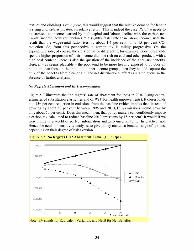
Figure 5.3 illustrates the “no regrets” rate of abatement for India in 2010 (using centralestimates of substitution elasticities and of WTP for health improvements). It correspondsto a 15+ per cent reduction in emissions from the baseline (which implies that, instead ofgrowing by about 80 per cent between 1995 and 2010, CO2 emissions would grow byonly about 50 per cent). Does this mean, then, that policy makers can confidently imposea carbon tax calculated to reduce baseline 2010 emissions by 15 per cent? It would if wewere living in a world of perfect information and zero uncertainty. … In practice, not.Hence the need for sensitivity analysis, to give policy makers a broader range of options,depending on their degree of risk aversion.

Figure 5.3: No Regrets CO2 Abatement, India (10^5 Rps)

Note: EV stands for Equivalent Variation, and NetB for Net Benefits

-4,000,000

-3,000,000

-2,000,000

-1,000,000

0

1,000,000

2,000,000

5 10 15 20 25 30

EVBenefitsNetB

Abatement Rate

35

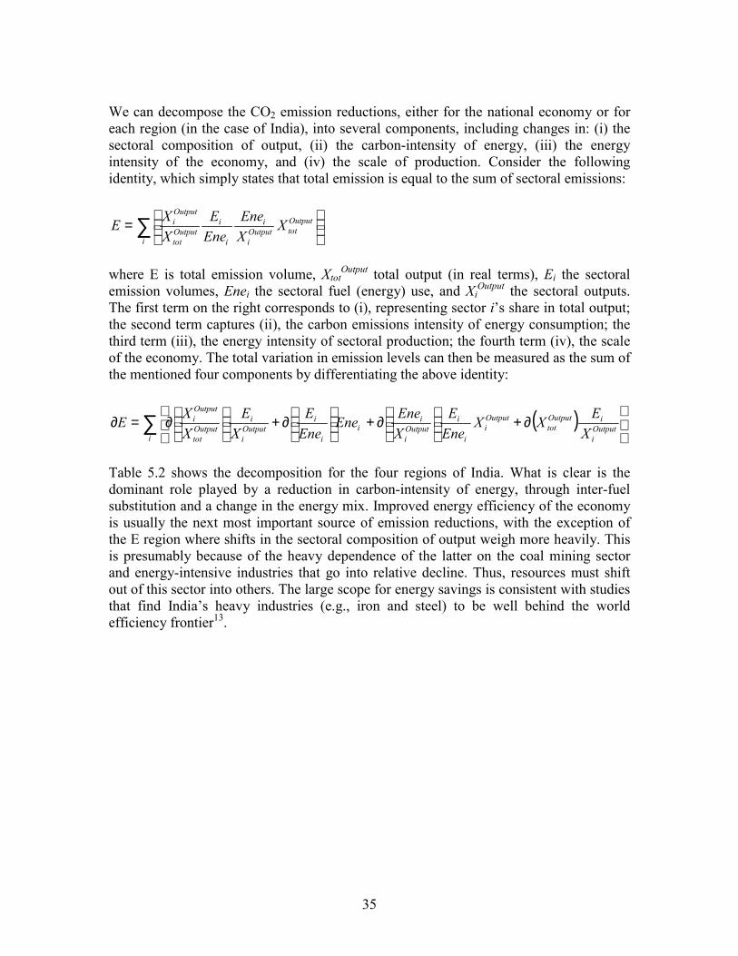
We can decompose the CO2 emission reductions, either for the national economy or foreach region (in the case of India), into several components, including changes in: (i) thesectoral composition of output, (ii) the carbon-intensity of energy, (iii) the energyintensity of the economy, and (iv) the scale of production. Consider the followingidentity, which simply states that total emission is equal to the sum of sectoral emissions:

∑

=

i

OutputtotOutput

i

i

i

iOutputtot

Outputi X

XEne

EneE

XXE

where E is total emission volume, XtotOutput total output (in real terms), Ei the sectoral

emission volumes, Enei the sectoral fuel (energy) use, and XiOutput the sectoral outputs.

The first term on the right corresponds to (i), representing sector i’s share in total output;the second term captures (ii), the carbon emissions intensity of energy consumption; thethird term (iii), the energy intensity of sectoral production; the fourth term (iv), the scaleof the economy. The total variation in emission levels can then be measured as the sum ofthe mentioned four components by differentiating the above identity:

( )∑

∂+

∂+

∂+

∂=∂

iOutputi

iOutputtot

Outputi

i

iOutputi

ii

i

iOutputi

iOutputtot

Outputi

XEXX

EneE

XEneEne

EneE

XE

XXE

Table 5.2 shows the decomposition for the four regions of India. What is clear is thedominant role played by a reduction in carbon-intensity of energy, through inter-fuelsubstitution and a change in the energy mix. Improved energy efficiency of the economyis usually the next most important source of emission reductions, with the exception ofthe E region where shifts in the sectoral composition of output weigh more heavily. Thisis presumably because of the heavy dependence of the latter on the coal mining sectorand energy-intensive industries that go into relative decline. Thus, resources must shiftout of this sector into others. The large scope for energy savings is consistent with studiesthat find India’s heavy industries (e.g., iron and steel) to be well behind the worldefficiency frontier13.

36

Uncertainty and Sensitivity Analysis

Sensitivity analysis is performed to determine how dependent results are on the particularvalues of certain key parameters and exogenous variables used in the simulations. Thereare any number of sensitivities one could test, but theory-informed intuition is used toselect the few thought to be most important. These are the substitution elasticities14 in theproduction function and the WTP values. (A proto-sensitivity-analysis was performedabove for the elasticity of WTP with respect to income – see Table 4.1, so that parameteris not treated further.) In a longer-term exercise, one would also be interested in testingalternative time paths of emission reductions. It is worth noting that the introduction ofancillary benefits into the analysis of climate policy may significantly alter the standardresult that “it pays to wait” because of the prospect of future technological improvementsthat will lower the costs of abatement. Now, these benefits of waiting need to be weighedagainst the costs in terms of additional lives lost and poor health in the here and now.

Clearly the fact that we employ sensitivity analysis at all suggests that we are uncertainabout the “true” values of certain parameters. Thus, in conducting the analysis, it wouldmake sense to choose alternative values that bound a range of plausible estimates.Ideally, this would involve specifying a statistical distribution such that one can assign aspecific probability to observing parameter values within the chosen range (e.g., 95%,99%). This is not always possible (requiring at a minimum information about thestandard deviation around a sample mean). In that event, more arbitrary rules can be used– e.g., multiplying substitution elasticity values by 0.5 and 1.5. This is what was done inthe case of India. In the case of VSL, the lower and upper bounds of the range of plausible

Table 5.2: Decomposition of CO2 Emission Changes, India by Region

5Share of total CO2 reduction attributableto change in: Nor Wes Sou EnoSectoral composition 10.2 6.3 7.0 21.6Carbon-intensity of energy 65.9 71.2 68.5 55.7Energy-intensity of output 17.4 16.2 18.7 16.2Scale of production 6.4 6.3 5.9 6.5

10Nor Wes Sou Eno

Sectoral composition 11.3 7.1 7.7 23.2Carbon-intensity of energy 65.2 70.2 68.2 54.7Energy-intensity of output 16.7 15.9 17.7 15.2Scale of production 6.8 6.8 6.3 6.9

15Nor Wes Sou Eno

Sectoral composition 11.6 7.4 7.9 23.5Carbon-intensity of energy 65.1 69.6 68.2 54.9Energy-intensity of output 16.1 15.6 17.1 14.4Scale of production 7.3 7.4 6.8 7.2

Abatement rate (%)

37

India-specific estimates15 was taken for the sensitivity analysis (the mid-point of thatrange being the central VSL value employed) (see Bussolo and O’Connor 2001).

Figure 5.4 presents the combined results of a series of sensitivity analyses in which, first,substitution elasticities in production were allowed to vary, holding WTP constant atcentral values, then WTP was varied, holding substitution elasticities constant at defaultvalues, then both substitution elasticities and WTP were allowed to vary. The “lowelasticity, low WTP” results in the first panel are the least favourable to “no regrets”climate policy, while the “high elasticity, high WTP” results are most favourable. Thedashed vertical lines through the horizontal axis show the “no regrets” abatement ratesassociated with each. Even in the least favourable case, the “no regrets” abatement rate isin the 10-15 per cent reduction range relative to baseline 2010 emissions. Ten per cent,then, would appear to be a “safe lower limit” on CO2 abatement for a risk-averse Indianpolicy maker. It should be noted that, if we were to include other greenhouse gases in theanalysis, the “safe lower limit” would in all likelihood be raised insofar as other gasesoffer low cost abatement options over some range16.

5.3. COMPARISON WITH OTHER RESULTS

We have presented the results generated by the CGE-based policy simulations, but arethese reasonable? What is our point of reference? There are several markers one can usefor cross-checking results, to see if they fall within a plausible range. (A caveat of suchcomparisons is that it might just be that all the previous studies produced erroneousresults.) The most common metrics for the economic analysis of climate policy are: themarginal cost of reducing a tonne of carbon (tC) (hence, the carbon tax rate) and, in thecase of ancillary benefits, the size of those benefits per tC reduction. The latter, in turn,can be measured either in physical units (e.g., premature deaths avoided or, put simply,lives saved per unit C reduction) or in monetary units. Our focus here is on the ancillarybenefits comparison.

In making cross study (and especially cross-country) comparisons of ancillary benefits, itis important to bear in mind the several possible sources of variance in results, includingdifferences in: underlying parameter values or variable estimates – e.g., of VSL; methodof estimating benefits (e.g., damages avoided versus abatement costs avoided); scope ofbenefits included (e.g., some studies include both emission-related benefits and non-emission-related ones like reductions in traffic congestion, accidents, and noise resultingfrom reduced road transport); population exposure to pollution across study sites.

Table 5.3 summarises calculations based on several studies that have looked at mortalitybenefits from climate policy. Our results show lives saved per million tonnes of carbonabated equal to 334, compared with 298 for China estimated by Garbaccio et al. Thenumbers for Chile and the United States are considerably lower. These relativemagnitudes are broadly consistent with the hypothesis state above that developingcountries with few initial local pollution controls (hence, little delinking of CO2emissions from other pollutants) are likely to benefit more climate policy – in terms oflives saved per tC reduction – than developed countries where such delinking is more

38

advanced. Another explanation for the high number of lives saved in China and India isthe high urban population densities, hence, the large exposed populations relative to Chileand the U.S.A.

Figure 5.4: Outer Bounds on "No

Low Elasticities, Low WTP

High Elasticities, High WTP

-5,000,000

-4,000,000

-3,000,000

-2,000,000

-1,000,000

0

1,000,000

2,000,000

5 10 15 20 25 30EVBenefitsNetB

-5,000,000

-4,000,000

-3,000,000

-2,000,000

-1,000,000

0

1,000,000

2,000,000

5 10 15 20 25 30EVBenefitsNetB

Regrets”

39

Table 5.3: Comparison of Mortality Benefits Estimates of CO2 Reductions

Study Lives saved per MtC reduction

Scenario Assumptions

Bussolo and O’Connor (2001) 334 India, 201015% CO2 reduction

Garbaccio et al. (2000) 298 China, 2010:10% CO2 reduction

Dessus and O’Connor (1999) 100 Chile, 2010:10% CO2 reduction

Cifuentes et al. (1999) 89 Chile, 2020:13% CO2 reduction

Abt Associates (1997) 82 USA, 2010:15% CO2 reduction

Source: O’Connor (2000); Bussolo and O’Connor (2001).

These health benefits of climate policy can also be expressed in value terms. Even if inIndia the number of premature deaths averted per tC abated is quadruple that in theUnited States, in value terms the difference will be smaller, given India’s much lower percapita income, hence willingness (capacity) to pay for cleaner air. The ancillary benefitsper tC abated in India come to around $58 (at 1995 exchange rate). This compares withone early U.S. estimate of around $26/tC from emission reductions in two sectors17 –transport and electricity – which together account for about two-thirds of carbonemissions (Ayres and Walter 1991). A more recent review for the U.S.A. by Burtraw andToman (1997) reports on the results of eight studies whose mean estimate of ancillarybenefits is virtually identical to the Ayres and Walter figure, with a low estimate ofaround $3 and a high of $8918.

European ancillary benefit estimates tend to be higher than those for the United States,reflecting in part higher population exposure (due to higher urban population densitiesand prevailing winds that blow pollution inland in Europe but out to sea from the easternUnited States). Considering only emission-related benefits, the values range (in 1990$US) from a low of $20/tC (Barker, 1993, for the U.K., based on social preferencesrevealed from the marginal costs of implementation of existing abatement technologies)to a high of $212/tC (Alfsen et al.1992, for Norway; Pearce 1992 reports a similar figurefor the U.K.: $195/tC). A mean value of emission-related benefits, based on the estimatesreported in Ekins (1995), is around $100/tC. A more recent Europe-wide assessment(Barker and Rosendahl, 2000) for the first Kyoto Protocol control period (2008-2012)finds average ancillary benefits per tC equivalent of around $125 (at 2000 prices andexchange rate). These benefits amount to between 15 and 40 per cent of the change inGDP brought about by GHG mitigation measures, depending on the European country.

40

6. CONCLUDING OBSERVATIONS

This paper has laid out the theory, methodology and some empirical results from the useof economy-wide models to compare ancillary benefits to the primary costs of climatepolicy in developing countries. A few results bear repeating.

First, the top-down modelling approach depends on the question at hand: it is best suitedto providing broad guidance to national policy makers who are concerned principallywith the economic costs of a carbon constraint. By integrated ancillary benefits into aconsistent modelling framework, it is possible to estimate the “no regrets” level ofabatement effort.

Second, the hypothesis seems to be borne out that countries that have undertakenrelatively little prior abatement of local air pollution stand to reap larger ancillary benefitsof climate policy than countries that have. While this does not always break down alongdeveloping/developed country lines, the environmental Kuznets curve observed in someof the data on pollution levels vs. per capita income suggests this is probably a good firstapproximation.

Third, this still leaves open the question of whether a country could get more for itsmoney, in terms of local pollution-related health benefits, by focusing on local air qualitytargets rather than on greenhouse gas reductions. Limited evidence suggests that theremay be tradeoffs but that there can be considerable coincidence between cost-effectivelocal pollution control measures and cost-effective GHG control measures. In any event,the intent of the analysis is not to suggest that policy makers ought to focus on climatepolicy first. Rather, it is to call their attention to (and attempt to quantify) previouslyoverlooked or undervalued benefits of such policy, while fully recognising that theirpriorities may well lie with local air pollution. In any event, the question of theconsistency of orderings between local abatement and global abatement cost-effectiveness is an area requiring more country-specific research.

Fourth, the evidence suggests that, while dose-response function transfer from developedto developing countries is justifiable for mortality from particulates exposure, it is moreproblematic where the endpoint being measured involves an explicit behaviouralcomponent, like self-medication, clinic visits, or hospital admissions. Even moreproblematic is transfer of WTP/VSL estimates, especially given the sensitivity of thederived value for the target site to the assumed income elasticity of WTP, on whichempirical evidence to date is far from consistent.

Fifth, there is a sense of incompleteness in an analysis that considers only the ancillary(not the primary) benefits of climate policy – bearing in mind that costs are simplynegative benefits and that some countries might gain on net from climate change. Therationale for this focus has been that developing country policy makers are likely todiscount heavily the distant future and highly uncertain primary benefits, while theancillary ones are far more certain and immediate. Still, in the final analysis, allsignificant costs and benefits will need to be compared, as will the timing of controls.

41

REFERENCES

Abt Associates Inc. (1997), “International PM Mortality Impacts in 2020 fromGreenhouse Gas Policies”, Memo from Leland Deck and Jennifer Jones, Abt, toDwight Atkinson and Tracey Woodruff, US EPA, dated 26 November.

Alberini, A., M. Cropper, T.-T. Fu, A. Krupnick, J.-T. Liu, D. Shaw, and W. Harrington(1997), “Valuing Health Effects of Air Pollution in Developing Countries: TheCase of Taiwan”, Journal of Environmental Economics and Management, 34:107-126.

Alfsen, K.H., A. Brendemoen, and S. Glomsrod (1992), “Benefits of climate policies:Some tentative conclusions”, Discussion Paper No. 69, Central Bureau ofStatistics, Oslo, Norway, March.

Armington, P. (1969), “A Theory of Demand for Products Distinguished by Place ofProduction”, IMF Staff Papers, 16: 159-178.

Aunan, K., T.K. Berntsen, and H.M. Seip (2000), “Surface Ozone in China and ItsPossible Impact on Agricultural Crop Yields”, Ambio, 29(6), September 294-301.

Ayres, R.U., and J. Walter (1991), “The Greenhouse Effect: Damages, Costs andAbatement”, Environmental and Resource Economics, 1: 237-270.

Barker, T. (1993), “Secondary Benefits of Greenhouse Gas Abatement: The Effects of aUK Carbon-Energy Tax on Air Pollution”, Nota di Lavoro 32.93, FondazioneENI Enrico Mattei, Milan.

Barker, T., and K.E. Rosendahl (2000) “Ancillary Benefits of GHG Mitigation in Europe:SO2, NOx, and PM-10 reductions to meet Kyoto targets using the E3ME modeland EXTERNE valuations”, in OECD, op.cit., pp. 413-451.

Baumol, W.J., and W.E. Oates (1988), The Theory of Environmental Policy, CambridgeUniveristy Press, Cambridge.

Beghin, J., B. Bowland, S. Dessus, D. Roland-Holst, and D. van der Mensbrugghe(1999), “Trade Integration, Environmental Degradation, and Public Health inChile: Assessing the Linkages”, 11 May, processed.

Beghin, J., S. Dessus, D. Roland-Holst, and D. van der Mensbrugghe (1996), “GeneralEquilibrium Modelling of Trade and the Environment”, Technical Paper No. 116,OECD Development Centre, Paris, September.

Bowland, B.J., and J.C. Beghin (1998), “Robust Estimates of Value of a Statistical Lifefor Developing Economies: An Application to Pollution and Mortality inSantiago”, CARD Working Paper 99-WP 214, Center for Agricultural and RuralDevelopment, Iowa State University, Ames, December.

Boyd, R., K. Krutilla, and W.K. Viscusi (1995), “Energy Taxation as a Policy Instrumentto Reduce CO2 Emissions: A Net Benefit Analysis”, Journal of EnvironmentalEconomics and Management, 29: 1-24.

Brandon, C., and K. Hommann (1995), “The Cost of Inaction: Valuing the Economy-wideCost of Environmental Degradation in India”, Asia Environment Division, WorldBank, 17 October, processed.

Burniaux, J.-M. (2000), “A Multi-Gas Assessment of the Kyoto Protocol”, EconomicsDepartment Working Paper No. 270, OECD, Paris, 2 November, processed.

42

Burniaux, J.-M., G. Nicoletti and J. Oliveira-Martins (1992), "GREEN: a Global Model forQuantifying the Costs of Policies to Curb CO2 Emissions", OECD Economic Studies, 19:49-92.

Burtraw, D., and M. Toman (1997), “The Benefits of Reduced Air Pollutants in the U.S.from Greenhouse Gas Mitigation Policies”, Discussion Paper 98-01, Resourcesfor the Future, Washington, D.C.

Bussolo, M., M. Chemingui, and D. O’Connor (2001), “A Multi-Region SocialAccounting Matrix (1995) and Regional Environmental General EquilibriumModel for India (REGEMI)”, OECD Development Centre WebDoc #1,forthcoming.

Bussolo, M., and D. O’Connor (2001), “Clearing the Air in India: The Economics ofClimate Policy with Ancillary Benefits”, OECD Development Centre TechnicalPaper No. 182, November, Paris.

Chameides, W.L., H. Yu, S.C. Liu, M. Bergin, X. Zhou, L. Mearns, G. Wang, C.S.Kiang, R.D. Saylor, C. Luo, Y. Huang, A. Steiner, and F. Giorgi (1999), “Casestudy of the effects of atmospheric aerosols and regional haze on agriculture: Anopportunity to enhance crop yields in China through emission controls?”, PNAS,96(24): 13626-13633.

Chesnut, L.G., B.D. Ostro, and N. Vichit-Vadakan (1997), “Transferability of AirPollution Control Health Benefits Estimates from the United States to DevelopingCountries: Evidence from the Bangkok Study”, American Journal of AgriculturalEconomics, 79(5): 1630-1635.

Cifuentes, L.A., and L.B. Lave (1993), “Economic Valuation of Air Pollution Abatement:Benefits from Health Effects”, Annual Review of Energy and the Environment,18: 319-342.

Cifuentes, L.A., E. Sauma, H. Jorquera, and F. Soto (1999), “Co-controls BenefitsAnalysis for Chile: Preliminary estimation of the potential co-control benefits forChile”, COP-5 Progress Report, School of Engineering, Pontifical CatholicUniversity of Chile, October, revised 12 November.

Colls, J. (1997), Air Pollution: An Introduction, E&FN SPON, Chapman & Hall,London.

Cropper, M.L., N.B. Simon, A. Alberini, S. Arora, and P.K. Sharma (1997), “The HealthBenefits of Air Pollution Control in Delhi, India”, American Journal ofAgricultural Economics, 79(5): 1625-1629.

Dahl, C. (1995), “Demand for Transportation Fuels: A Survey of Demand Elasticities andTheir Components”, The Journal of Energy Literature, I(2): 3-27.

Dessus, S., and D. O’Connor (1999), “Climate Policy without Tears: CGE-BasedAncillary Benefits Estimates for Chile”, OECD Development Centre TechnicalPaper No. 156, Paris, November.

Dessus, S., and D. O’Connor (2001), “Climate Policy without Tears: CGE-BasedAncillary Benefits Estimates for Chile”, Environmental and Resource Economics,final revisions submitted in June.

Dessus, S., D. Roland-Holst, and D. van der Mensbrugghe (1994), “Input-based PollutionEstimates for Environmental Assessment in Developing Countries”, TechnicalPaper No. 101, OECD Development Centre, Paris.

43

Dockery, D.W., J. Schwartz, and J.D. Spengler (1992), “Air Pollution and DailyMortality: Associations with Particulates and Acid Aerosols”, EnvironmentalResearch, 59: 362-373.

Dowlatabadi, H. (1998), “Sensitivity of climate change mitigation estimates toassumptions about technical change”, Energy Economics, 20: 473-493.

Ekins, P. (1995), “Rethinking the Costs Related to Global Warming: A Survey of theIssues”, Environmental and Resource Economics, 6, pp.231-277.

EPA (1998), The Benefits and Costs of the Clean Air Act, 1970 to 1990, U.S.Environmental Protection Agency, Washington, D.C.

EPA (2000), Developing Country Case-Studies. Integrated Strategies for Air Pollutionand Greenhouse Gas Mitigation: Progress Report for the International Co-Control Benefits Analysis Program, November.

Eskeland, G.S., and T.N. Feyzioğlu (1997), “Is demand for polluting goods manageable?An econometric study of car ownership and use in Mexico”, Journal ofDevelopment Economics, 53: 423-445.

Eskeland, G.S., and J. Xie (1997), “Acting Globally while Thinking Locally: Is theGlobal Environment Protected by Transport Emission Control Programs?” WorldBank, Washington, D.C., processed.

Fankhauser, S. (1995), Valuing Climate Change, Earthscan, London.Freeman, A. M., III (1993), The Measurement of Environmental and Resource Values:

Theory and Methods, Resources for the Future, Washington, D.C.Garbaccio, R.F., M.S. Ho, and D.W. Jorgenson (2000), “The Health Benefits of

Controlling Carbon Emissions in China”, Kennedy School of Government,Harvard University, 16 March, processed.

Goulder, L.H., and S.H. Schneider (1999), “Induced technological change and theattractiveness of CO2 abatement policies”, Resource and Energy Economics, 21:211-253.

Hammitt, J.K., J.-T. Liu, and J.-L. Liu (2000), “Survival is a Luxury Good: TheIncreasing Value of a Statistical Life”, prepared for NBER Summer InstituteWorkshop on Public Policy and the Environment, Cambridge, MA, August.

Hettige, H., P. Martin, M. Singh, and D. Wheeler (1995), “The Industrial PollutionProjection System”, Policy Research Working Paper 1431, The World Bank,Washington, D.C., March.

IEA (1995), World Energy Outlook, Paris.Jorgenson, D.W., R.J. Goettle, P.J. Wilcoxen, and M.S. Ho (2000), The Role of

Substitution in Understanding the Costs of Climate Change Policy, The PewCenter on Global Climate Change, Washington, D.C., September.

Kolstad, C.D. (2000), Environmental Economics, Oxford University Press, Oxford.Kolstad, C.D., and M. Toman (2001), “The Economics of Climate Policy”, RFF

Discussion Paper 00-40REV, Resources for the Future, Washington, D.C., June,processed.

Krupnick, A.J. (2001), “How Much Will People Pay for Longevity?” Resources, Winter,142: 14-17.

Krupnick, A., K. Harrison, E. Nickell, and M. Toman (1996), “The Value of HealthBenefits from Ambient Air Quality Improvements in Central and Eastern Europe:

44

An Exercise in Benefits Transfer”, Environmental and Resource Economics, 7:307-332.

Liu, J.-T., J.K. Hammitt, J.-D. Wang, and J.-L. Liu (2000), “Mother’s Willingness to Payfor Her Own and Her Child’s Health: A Contingent Valuation Study in Taiwan”,Health Economics, 9: 319-326.

Lluch, C. (1973), “The Extended Linear Expenditure System”, European EconomicReview, 4: 21-32.

Loehman, E., and V.H. De (1982), “Application of Stochastic Choice Modelling toPolicy Analysis of Public Goods: A Case Study of Air Quality Improvements”,Review of Economics and Statistics, 64(3): 474-480.

Lvovsky, K., and G. Hughes (1998), “Addressing the Environmental Costs of Fuels inDeveloping Countries”, presented at First World Congress of Environmental andResource Economists, 25-27 June, Venice, Italy.

Lvovsky, K., G. Hughes, D. Maddison, B. Ostro, and D. Pearce (1999), EnvironmentalCosts of Fossil Fuels: A Rapid Assessment Method with Application to Six Cities,World Bank, processed.

Markandya, A. (1998), “The indirect costs and benefits of greenhouse gas limitations”,Handbook Reports: Economics of Greenhouse Gas Limitations, UNEPCollaborating Centre on Energy and Environment, Risø National Laboratory,Roskilde, Denmark.

McKibbin, W.J., and P.J. Wilcoxen (1995), “The Theoretical and Empirical Structure ofthe G-Cubed Model”, November, processed.

Mitchell, R.C., and R.T.Carson (1986), Valuing Drinking Water Risk Reduction Usingthe Contingent Valuation Method: A Methodological Study of Risks from THMand Giardia, Report to U.S. Environmental Protection Agency, Washington, D.C.

O’Connor, D. (2000), “Ancillary Benefits Estimation in Developing Countries: AComparative Assessment”, in OECD, op.cit., pp. 377-396.

OECD (2000a), “A Multi-Gas Assessment of the Kyoto Protocol”, Working Party No. 1on Macroeconomic and Structural Policy Analysis, 29 September, Paris.

OECD (2000b), Ancillary Benefits and Costs of Greenhouse Gas Mitigation. Proceedingsof an IPCC Co-Sponsored Workshop, held on 27-29 March 2000, in Washington,D.C., Organisation for Economic Co-operation and Development, Paris.

Ostro, B. (1994), “Estimating the Health Effects of Air Pollutants: A Method with anApplication to Jakarta”, World Bank Policy Research Working Paper No. 1301,May.

Ostro, B., J.M. Sanchez, C. Aranda, and G.S. Eskeland (1996), “Air Pollution andMortality: Results from a Study of Santiago, Chile”, Journal of Exposure Analysisand Environmental Epidemiology, 6(1): 97-114.

Pearce, D. (1992), “The Secondary Benefits of Greenhouse Gas Control” CSERGEWorking Paper 92-12, April (revised), processed.

Pearce, D. (2000), “Policy Frameworks for the Ancillary Benefits of Climate ChangePolicies”, in OECD, op. cit., pp.517-560.

Pearce, D. (2001), “How developing countries can benefit from policies to controlclimate change”, in L. Gómez-Echeverri (ed.), Climate Change and Development,Yale School of Forestry & Environmental Studies, New Haven, CT.

45

Roy, J., J. Sathaye, A. Sanstad, P. Mongia, and K. Schumacher (1999), “ProductivityTrends in India’s Energy Intensive Industries”, Ernest Orlando LawrenceBerkeley National Laboratory, April; published in The Energy Journal, 20(3): 33-61.

Schwartz, J. (1994), “Air pollution and daily mortality: A review and meta-analysis”,Environmental Research, 64: 36-52.

Shukla, P. (1996), “The Modelling of Policy Options for Greenhouse Gas Mitigation inIndia”, Ambio, 25:4, June, 240-248.

Simon, N.B., M.L. Cropper, A. Alberini, and S. Arora (1999), “Valuing MortalityReductions in India: A Study of Compensating Wage Differentials”, WorkingPaper No.2078, World Bank Policy Research Department, January.

Smith, K.R. (1993), “Fuel Combustion, Air Pollution Exposure, and Health: TheSituation in Developing Countries”, Annual Review of Energy and theEnvironment, 18: 529-66.

Tol, R.S.J. (1995), “The Damage Costs of Climate Change – Towards MoreComprehensive Calculations”, Environmental and Resource Economics, 5: 353-374.

Viscusi, W. K. (1993), “The Value of Risks to Life and Health”, Journal of EconomicLiterature, 31: 1912-1946.

Weitzman, M.L. (1974), “Prices vs. Quantities”, Review of Economic Studies, 41: 477-491.

WHO (1989), Management and Control of the Environment, WHO/PEP/89.1, Geneva.World Bank (1994), Chile. Managing Environmental Problems: Economic Analysis of

Selected Issues, 19 December (Report No. 13061-CH).

46

TECHNICAL APPENDIX: ELEMENTS OF THE MODEL STRUCTURE

This Appendix presents the basic mathematical structure of the production andconsumption sectors of the CGE models used in the analysis; also the determination ofaggregate investment . (See Bussolo et al. 2001 for further details.)

Production structure

Recall text Figure 2.2 that presents the production nesting.

At the top level, the producer chooses a mix of a value-added-plus-energy19 aggregate(QKEL) and an intermediate demand aggregate (ND). The optimisation problem takes thefollowing form:

Dj

Nj

KELj

KELj NPQP +min

subject to the production function:pjpipi

Dj

Nj

KELj

KELjj NaQaXP

,,, /1 ρρρ

+=

where PjKEL is the aggregate price of value added plus energy, Pj

N is the price of theintermediate aggregate, aj

KEL and ajN are the CES share parameters, and ρ is the CES

exponent. The exponent and the CES elasticity are related via this relationship:

σρ

ρ σσ

=−

⇔ = −11

1 .

Note that in the model, the share parameters incorporate the substitution elasticity usingthe following relationships:

( ) ( )σσ αα Nj

Nj

KELj

KELj aanda ==

Each subsequent production nest in Figure 2.2 is subject to an equivalent optimisationrule.

Consumption structure

Consumers under the ELES are assumed to maximise the following utility function:

max ln( ) lnU C SPi i i s

i

= − +

∑µ θ µ

subject to the budget constraint:

P C S YiC

id

i

+ =∑C is consumer spending, S is saving (in value), Yd is disposable income, PC are consumerprices, and µ and θ are the ELES parameters.20 The Engel aggregation condition requiresthe following constraints on the parameters µ:

47

µ µi si

+ =∑ 1

The following demand functions can be derived:

CP

Y Pi ii

Ci

djC

jj

= + −

∑θ µ θ

The usual interpretation of this demand function is that consumption is composed of twoparts. The first part has been referred to as the subsistence minimum (or floorconsumption), θ. The term in parenthesis represents residual income after subtractingexpenditures on the subsistence minima. Therefore the second part of consumption of anygiven sector’s output is a share of supernumerary income. Note that there is no minimalconsumption of savings, i.e., θs is 0. Savings can be determined via the budget constraint:

S Y P CdiC

ii

= −∑The income and price elasticities are given by the following formulae:

η µ µχ

ε θ µ

ii

d

iC

i

i

i

ii i

i

YP C

C

= =

= − −( )1 1

The income elasticity is equal to the ratio of the marginal propensity to consume good iout of supernumerary income, µ, over the average propensity to consume good i out ofincome.

Investment determinationAppendix Table 1 includes the equations for the closure of the saving and investmentaccount. The domestic India-wide value of investment – the product of investment priceindex PI, and the investment volume ITOT – is equal to domestic saving (households andgovernment savings) plus foreign saving, plus depreciation, less expenditure on buildingstock.

Appendix Table 1: Determination of Aggregate Investment (Exogenous Foreign Saving)

∑−+++=i

ASTOCKii

DEPRf

SAVFg

TOTh

TOTI XPAYSPSSIP

TOTIr

TOTr

Ir IPIP α=

fSAVF

f SPS =

48

NOTES

1 Pearce (2001) cites damage estimates for non-OECD countries from a doubling of atmospheric CO2equivalent concentration for non-OECD countries of between 1.6% of GNP (Fankhauser 1995) and 2.7%of GNP (Tol 1995).2 Biomass fuel is normally a by-product of another productive sector – whether agriculture, livestock, orforestry. While the marketed outputs of these sectors get reflected in the I/O tables, it is not legitimate toapply the same technical coefficients to these by-products.3 Dowlatabadi (1998) provides some illustrations of how endogenising technical change can affect theanalysis of optimal climate policy. For example, with induced technical change, postponing climate policysignificantly raises costs of achieving the agreed target by foregoing important learning opportunities.Goulder and Schneider (1999) extend this analysis, suggesting that (in the absence of prior R&D taxdistortions) induced technical change can increase the gross social costs of a given carbon tax, though thisis more than offset by increased benefits. Thus, the optimal level of abatement is higher. Vieweddifferently, for a given abatement target, the gross social costs are lower with induced technical changethan without.4 VSL can be alternately expressed as the value of a premature death avoided and is estimated by individualwillingness to pay (WTP) for small reductions in the risk of premature death from specific causes (whetheron-the-job accidents or pollution-related illness). Algebraically, VSL = Value of ∆risk/ ∆risk. So, forinstance, if the average WTP for a 1/100,000 reduction in the risk of premature death (say, associated witha 10µ/m3 reduction in PM10) is $50, then the VSL implied by that WTP is $50/(1/100,000), or $5 million.5 To illustrate the role of temperature and humidity, according to one estimate, concentrations of particulatematter from a fixed quantity of emissions in hot and dry regions are about one-third of what would beexpected from the same emissions under most other climatic conditions (Working Group 1997).6 Ideally, region- or city-specific information on atmospheric conditions can be found to determine thesefrequencies, but if not then certain “default” frequencies can be used as an approximation.7 Particle size is measured in terms of “aerodynamic diameter” and is given in units of microns (thousandsof a millimeter); thus PM10 refers to particles with diameter of 10 microns or less and PM2.5 has anequivalent interpretation.8 The relationship between PM10 and mortality is non-linear, however, with a change evaluated at 50 µg/m3

associated with a 1.4 per cent increase in mortality (i.e., closer to the U.S. means) and one evaluated at 150µg/m3 increasing mortality by 0.4 per cent.9 Likewise, a recent study for Santiago, Chile, revises down earlier estimates by Ostro of the particulatesdose-response relationship. While Cifuentes et al. (2000) broadly confirm the statistical significance of therelationship found by Ostro et al. (1996) for PM2.5–mortality, the dose-response coefficient is found to beonly about half as large, with the difference attributable to controls for seasonal effects.10 In the case of the United States and India, as of 1998 life expectancy at birth was 77 and 63 yearsrespectively; WDI Indicators CD-ROM of the World Bank.11 This raises the vexed question of whether a sample of Canadians is representative of anyone other than,well, a sample of Canadians ;).12 It is too early to present results of policy simulations for China, so the discussion in section 5 focuses juston health impacts.13 IEA (1995), for example, estimates India’s 1992 energy use per tonne crude steel at 0.94 toe, comparedto 0.34 in the Republic of Korea and 0.33 in Japan (Table 5.10).14 Roy et al. (1999) suggest, e.g., that while raising energy prices in India would be an effective carbonabatement policy, it could be costly given what they estimate to be relatively weak inter-input substitutionpossibilities. If a policy maker shared this assessment, then s/he might be interested in knowing the effectof assuming lower substitution elasticities than the central values used in Bussolo and O’Connor (2001).15 See, e.g., Brandon and Hommann (1995); Simon et al. (1999).16 See Burniaux (2000) for a multi-gas assessment of the Kyoto Protocol, in which the savings from abatingacross three gases rather than just CO2 averages $26/tCeq for the Annex I countries in 2010.17 The benefits estimates are based on the assumption of a 20% reduction in air pollution from 1978 levels.18 Burtraw and Toman propose a “rule-of-thumb” (for the United States) that ancillary benefits can beassumed to be roughly 30% of the cost of carbon reduction for low to moderate rates of abatement.Observing that over some range the marginal costs of GHG reductions are likely to be close to zero, they

49

conclude that the existence of ancillary benefits even as small as $3/tC could significantly increase thevolume of emissions reduction that is considered “no regrets” in the sense of having negative or zero netcost.19 Due to the crucial importance of energy in terms of pollution, the demand for energy has been separatedfrom the rest of intermediate demand, and incorporated in the value added nest.20 In the utility function, S needs to be deflated by an appropriate price, which would represent theconsumer spot price of future consumption. This price does not need to be specified for the model sincehousehold saving can be derived as a residual from the budget constraint. For welfare calculations, theconsumer price index, cpi, has been chosen as the saving deflator since there is no forward-lookingbehaviour in REGEMI.