Embed Size (px)
Citation preview
Estimates of the Open Economy NewKeynesian Phillips Curve for Euro Area
Countries ∗†
Fabio Rumler‡
First Draft: November 2004
Abstract
In this paper an open economy model of the New Keynesian PhillipsCurve incorporating three different factors of production, domesticlabor and imported as well as domestically produced intermediategoods, is developed and estimated for 9 euro area countries and theeuro area aggregate. This general model nests existing closed economyand open economy models as special cases. We find that structuralprice rigidity is systematically lower in the open economy specificationof the model than in the closed economy specification indicating thatwhen firms face more variable input costs they tend to adjust theirprices more frequently. However, when the model is estimated in itsgeneral specification including also domestic intermediate inputs, pricerigidity increases again compared to the open economy specificationwithout domestic intermediate inputs.
∗This paper has been written in the context of the Eurosystem Inflation PersistenceNetwork (IPN).
†I would like to thank Jordi Gali, Lars Sondergaard and the participants in the Eurosys-tem Inflation Persistence Network and in particular Hans Scharler for valuable commentsand discussions. The views expressed in this paper are those of the author and do notcommit in any way the Oesterreichische Nationalbank or the ECB. All errors are my ownresponsibility.
‡Oesterreichische Nationalbank, Economic Analysis Division, Otto Wagner Platz 3,A-1090 Vienna, Austria, E-Mail: [email protected].
1

1 Introduction
There is large evidence in the literature that the baseline New KeynesianPhillips Curve model with the labor share proxying real marginal cost asa driving variable of inflation can explain inflation dynamics in many largeindustrial economies reasonably well; see Gali and Gertler [6] and Sbordone[15] for the US, and Gali, Gertler and Lopez-Salido [7], McAdam and Willman[12] for the Euro Area and Balakrishnan and Lopez-Salido [1] for the UK.
However, a number of studies have also shown that the baseline model isnot always appropriate in tracking inflation dynamics in particular for openeconomies, see Balakrishnan and Lopez-Salido [1] for the UK, Bardsen et al.[2] for European countries, Freystatter [5] for Finland, and Sondergaard [17]for Germany, France and Spain. Reduced form estimates for the marginalcost term in the baseline model are often found to be insignificant in thesestudies.
In this paper the baseline model is extended in order to account for openeconomy effects as well as effects of intermediate goods in the productiontechnology of the firm. Real marginal cost as a driving variable for inflationis decomposed into the relative prices of 3 different factors of production:real unit labor costs and the prices of imported and domestically producedintermediate goods. The formulation of our general model including importedas well as domestically produced intermediate inputs in production nestsexisting closed and open economy models of the hybrid NKPC.
The model is then estimated for the closed economy case, the case withonly imported intermediate inputs and in the general formulation with im-ported and domestically produced intermediate inputs in different specifica-tions for 9 euro area countries and the euro area aggregate with data from1970 to 2003 Q2 (for some countries shorter or longer time series are avail-able). We find that the degree of structural price rigidity as measured by theCalvo probability of changing a price is systematically higher for the closedeconomy case than in the open economy case with only imported interme-diate inputs in production. This could be explained by the fact that whenfirms face more variable input costs as they import from volatile internationalmarkets they tend to adjust their prices more frequently. When comparingthe the open economy case with only imported intermediate inputs and themost general specification with imported and domestically produced inter-mediate inputs structural price rigidity is found to be systematically higherin the latter case. This could be due to substitution of imported by domes-tic intermediate goods when the relative price of the former increases, thusmitigating the need for the firm to adjust prices.
2
This paper is structured as follows. Section 2 introduces the theoreticalmodel with monopolistically competitive firms employing three different in-put factors in the production of their output which is then used by consumersas final demand and by other firms as intermediate input. The open economyhybrid NKPC is derived from the profit maximization problem of the firmunder the Calvo pricing assumption. The model is then applied to the dataof 9 euro area countries and the euro area aggregate. Issues on the empiri-cal implementation of the model, in particular the different specifications forwhich the model is estimated, are discussed and the results of the estimationsare presented and interpreted in section 3. Finally, section 4 concludes thepaper.
2 The Model
The open economy New Keynesian Phillips Curve is derived form an openeconomy model in which international trade takes place at two levels of pro-duction. Monopolistically competitive firms sell their products to consumersat home and abroad as well as to domestic and foreign firms for their useas intermediate input. So, the representative firm’s output is used partly fordomestic and foreign final demand and partly as intermediate input in theproduction of domestic and foreign firms. The production technology of afirm includes domestic labor, foreign and domestically produced intermediategoods as factors of production such that the relative prices of these factorsaffect marginal costs of production. The firm’s price setting behavior is de-rived from the maximization of future discounted profits assuming Calvo [4]type pricing, i.e. firms are allowed to reset their price after a random intervalof time. In addition, we assume that within the group of Calvo price setterssome follow a rule of thumb updating their prices with past inflation whilethe rest sets its price optimally which gives rise to a hybrid open economyNKPC. The model is based on the line of research started by Gali and Gertler[6] and Gali, Gertler and Lopez-Salido [7] on the hybrid specification of theNKPC. It draws heavily on the open economy NKPC model of Leith andMalley [11] extending their model by introducing a third factor of produc-tion, i.e. domestically produced intermediate goods. Related models alsospecifying a variant of the open economy NKPC are in Balakrishnan andLopez-Salido [1], Razin and Yuen [14] and Gali and Lopez-Salido [8].
3

2.1 Product Demand
In our open economy model consumers derive their utility from a consump-tion bundle including domestic and foreign consumption goods:
Ct =
[χ
1η
(cdt
) η−1η + (1 − χ)
1η
(cft
) η−1η
] ηη−1
(1)
where cdt =
[∫ 10 cd
t (z)ε−1
ε dz] ε
ε−1
and cft =
[∫ 10 cf
t (z)ε−1
ε dz] ε
ε−1
are again
CES indices of consumption goods produced in the home and foreign country,ε is the elasticity of substitution of goods within one country and η theelasticity of substitution of consumption bundles between countries and χis the parameter representing the home bias in consumption. By assumingε 6= η we allow the substitutability of goods within countries to differ fromthe subsitutatbility of goods across countries.1
The associated consumption price index which minimizes the cost of pur-chasing one unit of the composite consumption bundle Ct is given by
Pt =[χ(pd
t
)1−η+ (1 − χ)
(pf
t
)1−η] 1
1−η
(2)
where also pdt =
[∫ 10 pd
t (z)1−ε dz] 1
1−ε and pft = et
[∫ 10 p∗ft (z)1−ε dz
] 11−ε are
the price indices associated with domestic and foreign production (in domes-tic currency), et being the nominal exchange rate (where foreign variablesare denoted with an asterisk).
In addition to domestic and foreign consumers, the product of each indi-vidual firm is also demanded by domestic and foreign producers as interme-diate input in their production. So, the output of each firm is partly used forfinal consumption and partly as intermediate inputs by other firms. Accord-ingly, the bundles of domestically produced goods used in domestic and for-
eign production as intermediate inputs are defined by mdt =
[∫ 10 md
t (z)ε−1
ε dz] ε
ε−1
and m∗dt =
[∫ 10 m∗d
t (z)ε−1
ε dz] ε
ε−1
where the degree of substitutability between
intermediate goods is assumed to be the same as between consumption goods.Given that domestic and foreign consumers and domestic and foreign
producers all demand the product of each individual firm and allocate their
1see Tille [18]. Most other contributions like the well known paper by Obstfeld andRogoff [13] focus on the case where ε = η. In our application, however, η appears onlyimplicitly in the NKPC and does not feature as a structural paramter to be estimated orcalibrated.
4
demands for consumption and intermediate goods across countries and prod-ucts with the same pattern, the global demand for the output of firm z isgiven by2
ydt (z) =
(pd
t (z)
pdt
)−ε (cdt + c∗dt + md
t + m∗dt
)(3)
The demand for the firm’s product depends on the price charged by thefirm relative to the other domestically produced goods and the total demandof domestic and foreign consumers as well as producers allocated to domesticgoods.
2.2 Production Technology
Each individual firm produces its output employing labor and domestic aswell as foreign intermediate goods as variable factors of production and afixed amount of capital
yt (z) =(αNNt (z)
ρ−1ρ + αdm
dt (z)
ρ−1ρ + αfm
ft (z)
ρ−1ρ
) ρ(ρ−1)φ
K1− 1
φ (4)
where Nt(z), mdt (z) and mf
t (z) are domestic labor, domestically producedand imported intermediate inputs used in production by firm z and αN , αd
and αf are the weights of these factors in the production function. Theinputs enter the production function as imperfect substitutes where ρ is theconstant elasticity of substitution between them and 1 − 1
φrepresents the
weight of capital in production.To derive marginal costs from this production function we note that the
variable factors of production when combined with fixed capital display de-creasing marginal returns which induces an increasing marginal cost functionand thus a dependence of marginal costs on firm specific output. Firm spe-cific real marginal costs of firm z can then shown to be
2Implicitly consumers and input demanding firms pursue a 2-step optimization by firstallocating their demand across countries, which in the case of the domestic demand fordomestically produced consumption goods yields cd
t = (pdt /Pt)−ηχCt, and in a second step
within a country, which in the case of the demand for a specific domestic firm’s consump-tion good yields cd
t (z) = (pdt (z)/pd
t )−εcd
t with cdt being given by the above expression. The
total demand for a domestic firm’s output is then the sum of the demand for its consump-tion good at home and abroad, cd
t and c∗dt (for which an equivalent expression can be
found), as well as for its output employed as intermediate input by domestic and foreignfirms, md
t and m∗dt , which leads to expression 3.
5

MCt (z) = φ
[WtNt (z) + pd
t mdt (z) + pf
t mft (z)
Ptyt (z)
](5)
2.3 Price Setting
Firms set their prices by maximizing real variable profits facing the con-straints implied by Calvo contracts in that they can only change their pricesafter a random interval of time. Specifically, firms are allowed to change theirprice with a fixed probability 1 − θ in a given period while they keep theirprice constant with probability θ. Thus, when deriving the profit maximiz-ing price firms take into account that the price may be in effect for a longperiod of time and therefore discount future profits with the probability θ.The optimization problem of the firm in period t can then be written as
Πt (z)
Pt
= Et
∞∑s=0
θs
[xt
Pt+s
(xt
pdt+s
)−ε
yt+s − MCt
(xt
pdt+s
)−εφ
yφt+s
]∏s
j=1 rt+j−1
(6)
where Πt(z) denotes variable profit of the firm, xt is the newly set optimalprice, yt+s summarizes total demand for domestic goods (cd
t+s + c∗dt+s +mdt+s +
m∗dt+s) from the demand function 3, MCt is the part of real marginal cost
that is not firm specific3 and rt is the stochastic discount rate.Since under the Calvo pricing assumption only a fraction of firms are
allowed to reset their price every period, the index of output prices can beshown - by making use of the Law of Large Numbers - to be a weightedaverage of prices reset in period t and the previous period’s price index(
pdt
)1−ε= θ
(pd
t−1
)1−ε+ (1 − θ) (pr
t )1−ε (7)
where p rt is the reset price in period t. In addition to pure Calvo pricing
we also assume that within the group of firms who are allowed to reset itsprice in a given period a fraction of firms do not set their prices based onthe optimization but instead follow a simple rule of thumb. This deviationfrom optimality by part of the firms is common in the literature and can berationalized by costs of price adjustment (not modeled here) which become
3MCt(z) can be shown to equal φyt(z)φ−1MCt where MCt is a function of the prices ofthe factors of production and the parameters in the production function that are commonto all firms.
6
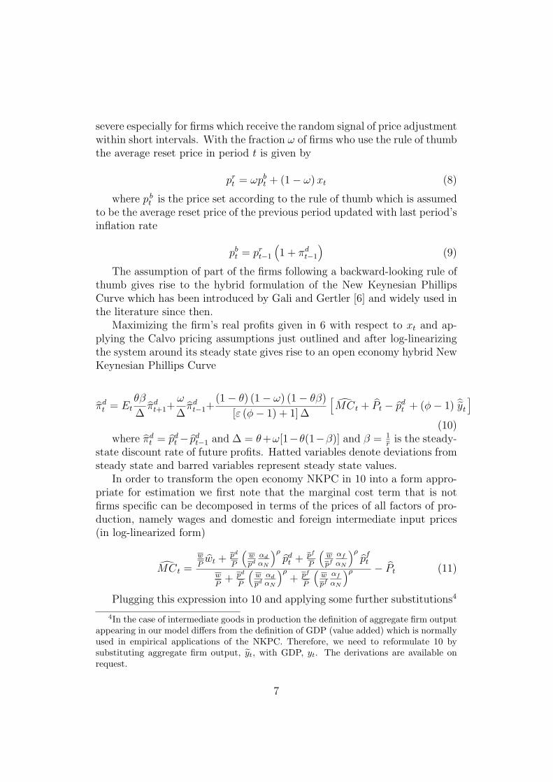
severe especially for firms which receive the random signal of price adjustmentwithin short intervals. With the fraction ω of firms who use the rule of thumbthe average reset price in period t is given by
prt = ωpb
t + (1 − ω) xt (8)
where p bt is the price set according to the rule of thumb which is assumed
to be the average reset price of the previous period updated with last period’sinflation rate
pbt = pr
t−1
(1 + πd
t−1
)(9)
The assumption of part of the firms following a backward-looking rule ofthumb gives rise to the hybrid formulation of the New Keynesian PhillipsCurve which has been introduced by Gali and Gertler [6] and widely used inthe literature since then.
Maximizing the firm’s real profits given in 6 with respect to xt and ap-plying the Calvo pricing assumptions just outlined and after log-linearizingthe system around its steady state gives rise to an open economy hybrid NewKeynesian Phillips Curve
πdt = Et
θβ
∆πd
t+1+ω
∆πd
t−1+(1 − θ) (1 − ω) (1 − θβ)
[ε (φ − 1) + 1] ∆
[MCt + Pt − pd
t + (φ − 1) yt
](10)
where πdt = pd
t − pdt−1 and ∆ = θ+ω[1−θ(1−β)] and β = 1
ris the steady-
state discount rate of future profits. Hatted variables denote deviations fromsteady state and barred variables represent steady state values.
In order to transform the open economy NKPC in 10 into a form appro-priate for estimation we first note that the marginal cost term that is notfirms specific can be decomposed in terms of the prices of all factors of pro-duction, namely wages and domestic and foreign intermediate input prices(in log-linearized form)
MCt =
wPwt + pd
P
(wpd
αd
αN
)ρpd
t + pf
P
(wpf
αf
αN
)ρpf
t
wP
+ pd
P
(wpd
αd
αN
)ρ+ pf
P
(wpf
αf
αN
)ρ − Pt (11)
Plugging this expression into 10 and applying some further substitutions4
4In the case of intermediate goods in production the definition of aggregate firm outputappearing in our model differs from the definition of GDP (value added) which is normallyused in empirical applications of the NKPC. Therefore, we need to reformulate 10 bysubstituting aggregate firm output, yt, with GDP, yt. The derivations are available onrequest.
7
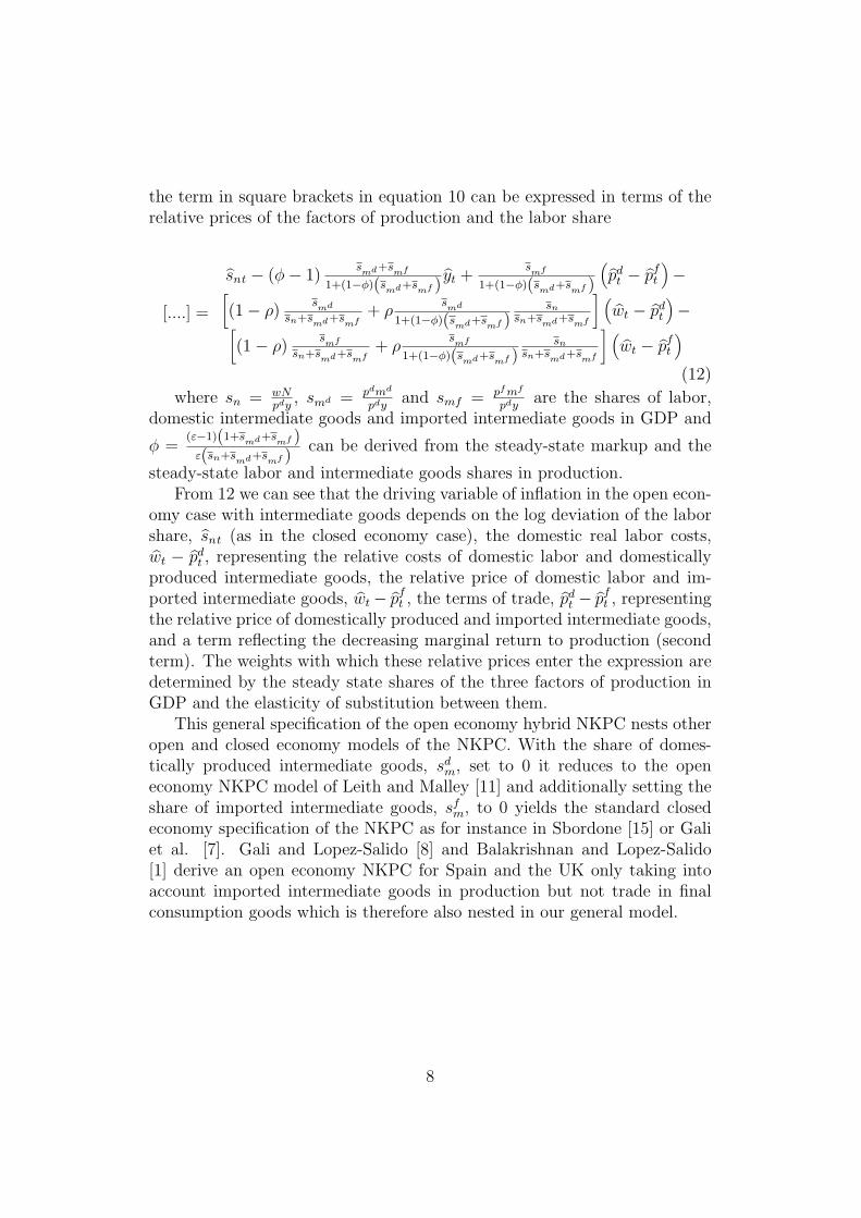
the term in square brackets in equation 10 can be expressed in terms of therelative prices of the factors of production and the labor share
[....] =
snt − (φ − 1)smd+s
mf
1+(1−φ)(smd+s
mf )yt +
smf
1+(1−φ)(smd+s
mf )
(pd
t − pft
)−[
(1 − ρ)smd
sn+smd+s
mf+ ρ
smd
1+(1−φ)(smd+s
mf )sn
sn+smd+s
mf
] (wt − pd
t
)−[
(1 − ρ)smf
sn+smd+s
mf+ ρ
smf
1+(1−φ)(smd+s
mf )sn
sn+smd+s
mf
] (wt − pf
t
)(12)
where sn = wNpdy
, smd = pdmd
pdyand smf = pf mf
pdyare the shares of labor,
domestic intermediate goods and imported intermediate goods in GDP and
φ =(ε−1)(1+s
md+smf )
ε(sn+smd+s
mf )can be derived from the steady-state markup and the
steady-state labor and intermediate goods shares in production.From 12 we can see that the driving variable of inflation in the open econ-
omy case with intermediate goods depends on the log deviation of the laborshare, snt (as in the closed economy case), the domestic real labor costs,wt − pd
t , representing the relative costs of domestic labor and domesticallyproduced intermediate goods, the relative price of domestic labor and im-ported intermediate goods, wt − pf
t , the terms of trade, pdt − pf
t , representingthe relative price of domestically produced and imported intermediate goods,and a term reflecting the decreasing marginal return to production (secondterm). The weights with which these relative prices enter the expression aredetermined by the steady state shares of the three factors of production inGDP and the elasticity of substitution between them.
This general specification of the open economy hybrid NKPC nests otheropen and closed economy models of the NKPC. With the share of domes-tically produced intermediate goods, sd
m, set to 0 it reduces to the openeconomy NKPC model of Leith and Malley [11] and additionally setting theshare of imported intermediate goods, sf
m, to 0 yields the standard closedeconomy specification of the NKPC as for instance in Sbordone [15] or Galiet al. [7]. Gali and Lopez-Salido [8] and Balakrishnan and Lopez-Salido[1] derive an open economy NKPC for Spain and the UK only taking intoaccount imported intermediate goods in production but not trade in finalconsumption goods which is therefore also nested in our general model.
8
3 Estimation and Results
3.1 The Data
The open economy New Keynesian Phillips Curve is estimated for 9 euro areacountries and the euro area aggregate. For Luxembourg, Ireland and Portu-gal the NKPC could not be estimated either due to the lack of appropriatedata or too short time series. The data for the estimation of the countryNKPCs have been obtained from two sources, the database of macroeco-nomic time series of the Inflation Persistence Network available on the IPNwebsite and from the New Chronos database provided by Eurostat. The datafor real and nominal GDP, the GDP deflator, compensation to employees,employment, real and nominal imports and the import deflator have beentaken from the IPN database and the data on intermediate inputs have beendownloaded from the national accounts database on New Chronos. Infor-mation on the share of imported intermediate goods in total imports havebeen calculated from input-output tables when available on the New Chronosdatabase. In case the input-output tables for some countries have been avail-able for more years (New Chronos reports input-output tables for 1995, 1997and 2000) the imported intermediate goods share has been averaged over theavailable years. The data on intermediate inputs which are available only atannual frequency have been disaggregated to quarterly frequency with thehelp of Ecotrim, a software for temporal disaggregation supplied by Eurostat.The shares of domestically produced and imported intermediate inputs, sd
m
and sfm, have been calculated as nominal intermediate inputs - decomposed
into domestic and imported shares - divided by nominal GDP and the laborshare, sn, is total compensation to employees divided by GDP.
3.2 Empirical Specification
We estimate the structural parameters of the model outlined in the previoussection employing a single equation approach. Equation 10 including 12 isestimated employing the generalized method of moments (GMM) estimatorproposed by Hansen [10] which has been widely used in solving the orthog-onality conditions implied by forward-looking rational expectations models- as in our model, see Verbeek [19]. The structural parameters which areestimated in our empirical specifications include θ, the probability that a
9

firm keeps a fixed price in a given period, β, the steady-state discount fac-tor of firms, ω, the fraction of firms following the rule of thumb and ρ, theelasticity of substitution between labor, domestic and imported intermedi-ate inputs in production. However, the elasticity of demand of the firm’sproduct, ε, cannot be estimated econometrically, as it does not appear in theestimation equation, but has to be calibrated in order to derive an empiricalvalue for the the elasticity of substitution between capital and the variablefactors of production, φ. In calibrating ε we follow the literature (see Gali etal. [7], Leith and Malley [11]) and adopt a value of 11 as a baseline implyinga steady-state markup of prices over marginal costs µ = ε
ε−1of 1.1.
One important point concerning the empirical implementation of our openeconomy NKPC is the choice of the price index for the dependent variabledomestic output inflation, πd
t . In the model the price set by a firm is itsoutput price. The output is then used for final consumption demand andintermediate inputs of other forms at home or abroad. Empirically, the ap-propriate index that measures aggregate output prices is the output deflator.However, output deflators are not available from current accounts statisticsfor the euro area countries. Another candidate as the empirical counter-part of aggregate output prices is the producer price index (PPI). There are,however, two considerations that limit the use of the producer price indexfor our estimations: First, also the producer price index for many euro areacountries is available only for too short time periods (e.g. for Austria onlysince 2000) and, second, it does not exactly measure output prices as definedin our model since it only measures prices at the industrial producer levelbut not at the final demand level. Given this and in order for our resultsto be comparable to other studies the value added (GDP) deflator has beenchosen as the dependent variable of our empirical model. While on concep-tual grounds it is clear that the value added deflator is not the appropriateindex to measure output prices, empirically, given the principle of double-deflation employed by statistical agencies in national accounts statistics, theoutput deflator and the value added deflator are not too different from eachother if a rapid pass-through from input to output prices is assumed5. Arapid pass-through is not an unrealistic assumption at the annual frequencyfor which the output deflator is usually measured and given the fact thatthe output deflator and the value added deflator display the same seasonalpattern as they are converted from annual to quarterly frequency with thehelp of the same indicator variables (e.g. wholesale prices, producer prices,CPI components) considering the GDP deflator in our estimations at the
5This has been verified for the Austrian case where the output deflator was directlyavailable.
10
quarterly frequency should not make any significant difference as comparedto the output deflator. Moreover, given that in our model the firm chargesthe same price for its output regardless if it is used for final demand or in-termediate inputs by other firms, the empirical price index used for the priceof domestically produced intermediate goods is also the GDP deflator6.
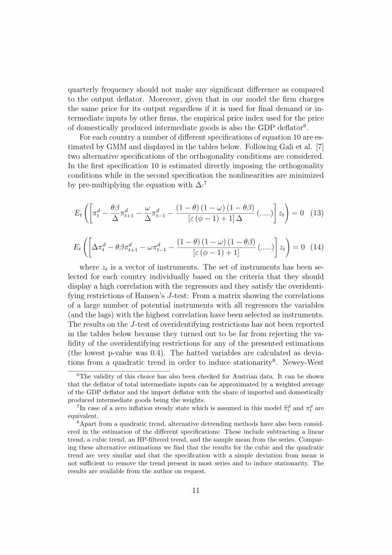
For each country a number of different specifications of equation 10 are es-timated by GMM and displayed in the tables below. Following Gali et al. [7]two alternative specifications of the orthogonality conditions are considered.In the first specification 10 is estimated directly imposing the orthogonalityconditions while in the second specification the nonlinearities are minimizedby pre-multiplying the equation with ∆:7
Et
([πd
t −θβ
∆πd
t+1 −ω
∆πd
t−1 −(1 − θ) (1 − ω) (1 − θβ)
[ε (φ − 1) + 1] ∆(.....)
]zt
)= 0 (13)
Et
([∆πd
t − θβπdt+1 − ωπd
t−1 −(1 − θ) (1 − ω) (1 − θβ)
[ε (φ − 1) + 1](.....)
]zt
)= 0 (14)
where zt is a vector of instruments. The set of instruments has been se-lected for each country individually based on the criteria that they shoulddisplay a high correlation with the regressors and they satisfy the overidenti-fying restrictions of Hansen’s J-test: From a matrix showing the correlationsof a large number of potential instruments with all regressors the variables(and the lags) with the highest correlation have been selected as instruments.The results on the J-test of overidentifying restrictions has not been reportedin the tables below because they turned out to be far from rejecting the va-lidity of the overidentifying restrictions for any of the presented estimations(the lowest p-value was 0.4). The hatted variables are calculated as devia-tions from a quadratic trend in order to induce stationarity8. Newey-West
6The validity of this choice has also been checked for Austrian data. It can be shownthat the deflator of total intermediate inputs can be approximated by a weighted averageof the GDP deflator and the import deflator with the share of imported and domesticallyproduced intermediate goods being the weights.
7In case of a zero inflation steady state which is assumed in this model πdt and πd
t areequivalent.
8Apart from a quadratic trend, alternative detrending methods have also been consid-ered in the estimation of the different specifications: These include subtracting a lineartrend, a cubic trend, an HP-filtered trend, and the sample mean from the series. Compar-ing these alternative estimations we find that the results for the cubic and the quadratictrend are very similar and that the specification with a simple deviation from mean isnot sufficient to remove the trend present in most series and to induce stationarity. Theresults are available from the author on request.
11
corrected standard errors which are robust to heteroskedasticity and auto-correlation of unknown form are employed in the coefficient’s significancetests. This correction is especially important when the variance of the de-pendent variable (inflation) changes over time, which for instance could bedue to one or more regime shifts of monetary or exchange rate policy in thesample period. The number of lags considered for the computation of thecoviarance matrix was based on a rule proposed by Newey-West dependingon the sample length (e.g. 4 lags for a sample of 120 quarters).
3.3 Results
The estimation results are summarized in tables 1 to 10 in the appendix. Alltables give the estimates of the structural parameters θ, β, ω and ρ alongwith the significance levels and report the expected duration of prices inmonths in the last column which has been derived from θ by the formula
31−θ
. The estimation results of the different model specifications are listedin the rows of the tables: In model M1 we estimate the specification for theclosed economy without intermediate inputs in production, i.e. the standardspecification of closed economy hybrid New Keynesian Phillips curve mod-els widely used in the literature, e.g. in Gali et al. [7] and others. ModelM2 includes imported intermediate goods in production but no domesticallyproduced inputs which is the specification adopted in the previous literatureon open economy NKPCs, as in Leith and Malley [11]. Model M3 is the mostgeneral formulation of the open economy NKPC as developed in this paper,as it includes domestic and imported intermediate inputs in production. Fur-thermore, the models with extension A are estimated according to the firstspecification mentioned above (equation 13) and the models with extensionB are based on the second specification (equation 14). In addition to thebaseline models of each class where the elasticity of substitution between thevariable factors of production, ρ, is freely estimated, a second specificationis displayed where ρ is restricted to 1, implying a Cobb-Douglas productionfunction. In the lower part of the table the estimates of the reduced formcoefficients are reported for those specifications (M1, M2, M3) where themarginal cost term was significant. Specifically, the reduced form coefficientsestimates along with their significance levels were obtained from the estima-tion of the following reduced form model (the notation follows Gali et al. [6])πd
t = Etγf πdt+1 + γbπ
dt−1 + λ [.....]. In the last row of each table the specific
instrument set that was used in the estimations of the different specificationsfor each country is listed.
12
In discussing the results we want to focus on some systematic findingsthat emerge from the comprehensive evidence on estimations of differentspecifications of the hybrid NKPC for 9 euro area countries and the euroarea itself. When screening the tables one striking results is the large degreeof heterogeneity in the estimated structural parameters of the price settingmodel across euro area countries but also across specifications for each coun-try. Concerning the estimated persistence of prices measured by both, θand ω, we realize that persistence seems to be highest in Germany and forthe euro area aggregate and lowest for Greece, the Netherlands and Finlandwhile the results for Spain, France and Italy are fairly similar displaying anintermediate degree of persistence. The fact that persistence is found tobe higher in countries with rather closed economies than in countries withrather open economies can be taken as a first indication that open economyconsiderations matter for the NKPC. When comparing the results with thoseof related studies and bearing in mind all the differences concerning instru-ments used and the sample length we find that they are more or less in linewith Gali et al. [7] and McAdam and Willman [12] for the euro area. Ourestimate for θ in the closed economy specification A of 0.78 is very similar to0.79 in Gali et al. and 0.8 in McAdam and Willman while the estimates forβ and ω are quite lower in Gali et al. but similar in McAdam and Willman.Comparing our results for Spain to those obtained by Gali and Lopez-Salido[8] we realize a considerable difference in that our estimates for θ and ω areconsistently lower and the estimates for β are consistently higher than inthe other paper for both, the closed economy as well as the open economyspecifications. There is, however, an important difference in the empiricalimplementation of the NKPC in that Gali and Lopez-Salido consider onlythe case of constant returns to labor in production while we assume de-creasing returns to labor (and imported intermediate goods). Compared toSondergaard [17] our results for Italy, France and Spain yield somewhat lowerestimates for the persistence parameter θ in the open economy specificationbut a comparison of the results between the two papers is difficult as theempirical implementation of the NKPC is rather different in Sondergaard(he uses other price indices and focuses on the traded sector only). Finally,our results for Germany, France and Spain are quite similar to the results inLeith and Malley [11] who estimate an open economy NKPC (correspondingto M2 in this paper) for the G7. In particular, the ranking of the three coun-tries with respect to price rigidity is the same in both papers with Germanyshowing the most rigid price setting behavior, followed by France and Spain.
Next we focus on the question if structural price rigidity as derived fromour results differs for different specifications of the same country. When com-paring the estimates of the “price rigidity parameter” θ between the closed
13
economy formulation M1 and the open economy formulation M2 a systematicdifference emerges of the form that price rigidity tends to be lower when im-ported intermediate prices are allowed to affect firm’s marginal costs.9 This isconsistent with the hypothesis that firms whose input prices vary more (duee.g. to volatile raw material prices) also adjust their prices more frequentlythan others. Exceptions from this tendency are Spain, Greece and Austriawhere the coefficients are basically unaffected by the introduction of openeconomy effects. The comparison of coefficients across models is summarizedin Table 11 which shows the difference in the estimates of θ and ω between M1and M2 in the first row of each country panel, the %-difference in parenthesisand the t-value for a t-test of statistically significant parameter difference ofnon-nested models10. Table 11 reveals that in 70% of all comparisons of M1and M2 (14 out of 20 total specifications, i.e. specification A and B for eachcountry) θ is higher for M1 than for M2, the average %-difference betweenthe two models is 15.8% but the difference is never statistically significantfor these 14 cases. There is only one statistically significant difference whencomparing θ between M1 and M2 for France in specification B, but the dif-ference goes the other direction, i.e. θM1 − θM2 < 0. In general it is veryhard to find significant results in Table 11 on the difference of coefficientsthat are bounded between 0 and 1 (most of them even vary within a muchsmaller range between 0.4 and 0.7 in the case of θ) but a difference of morethan 10% implying a difference in price duration of 1 to 2 months can beinterpreted to be at least economically significant.
Interestingly, when moving from the open economy specification M2 tothe most general model M3 - with imported and domestically produced in-termediate inputs - θ is systematically found be be higher than in M2, manytimes also higher than in the closed economy case. This could reflect substi-
9There is a discussion in the literature which parameter of the model appropriatelyindicates the degree of price rigidity in the case of a hybrid NKPC. Besides the probabilityof a price change, price rigidity can also be associated to the share of backward lookingfirms, ω, as they introduce some past-dependence in the pricing process. Based on thisreasoning, Benigno and Lopez-Salido [3] propose a formula that combines θ and ω to derivethe average duration between price changes: D = 1
1−θ1
1−ω . However, as this derivation isvalid only under certain assumptions and in order to be comparable to other studies wereport the implied duration between price changes in the conventional form D = 1
1−θ andinterpret θ as the parameter indicating price rigidity.
10The test statistic is θM1−θM2√σ2
θM1+σ2
θM2
where σθM1 and σθM2 are the standard deviations
of the coefficient estimates of θM1 and θM2. This test statistic is t-distributed with (n1 +n2−k1−k2) degrees of freedom where n1 and n2 are the number of observation underlyingthe estimation of M1 and M2, respectively, and k1 and k2 are the number of coefficientsto be estimated in M1 and M2.
14

tution of imported intermediate goods by domestic intermediate goods whenthe relative price of the former increases, thus mitigating the need to adjustprices for the firm. Table 11 reveals that in all but one cases (95%) θ in-creases from M2 to M3 and for 5 out of 10 countries even significantly. Theaverage %-difference between θ in M2 and M3 over all specifications is 24.7%.In 75% of the cases price rigidity as measured by θ in M3 is also higher thanin the closed economy specification M1, for 3 countries even significantly.
A similar pattern as has been described for θ can also be found for theparameter indicating the importance of backward-looking price setting ω: Itis found to be lower in the open economy specification than in the closedeconomy and the general specification M3, however the pattern is somewhatless systematic (in 65% of all comparisons between M2 and M3 ω is higher inM3). Contrary to the findings of Leith and Malley [11], these two parametersseem to be positively correlated across models in our analysis.
The estimates of the discount rate of firm’s future profits, β, are found tobe in a reasonable range between 0.9 and 1, in some cases even larger than 1but never significantly larger than 1. Compared to related studies, e.g. Leithand Malley [11] and Gali et al. [7], our estimates of β are much closer to 1which is also theoretically more plausible given that it reflects the quarterlysubjective discount rate of future profits. Furthermore, the estimates of βare not systematically affected by the specification of the model.
The elasticity of substitution between the variable factors of productionρ can only be estimated imprecisely, as it is found to be significant only invery few cases. This implies that - with exception of these few cases, e.g.M2B in France and M3B in Greece - assuming a Cobb-Douglas productionfunction, i.e. ρ = 1, would fit the data equally well.
When trying to assess which model (M1, M2 or M3) is most appropriateto characterize the inflation process in the euro area countries we turn tothe performance of the model estimated in its reduced form. The reason isthat when the reduced form coefficient on the marginal cost term λ cannotbe estimated significantly we have an identification problem of the structuralparameters of the model which then become unreliable (see Guay and Pelgrin[9]). Thus, the structural parameters of the model given in the tables are onlyconditional on a well specified reduced form. Comparing the reduced formcoefficients on the marginal cost term we note that the general model M3with imported and domestically produced intermediate inputs in productionand the model M2 with only imported intermediate goods in production arefound to be more appropriate to track the inflation process in all euro areacountries than M1 as λ was never found to be significant for M111 (remember
11The author will elaborate more on this issue in the next version of the paper.
15
that the reduced form specification is only reported in the tables for thosemodels where λ is significant). Thus, we conclude that open economy aspectsmatter for the performance and the fit of the NKPC.
It has to be noted also that for many countries differences in coefficientsestimates between specifications A and B are more pronounced than differ-ences between the model types M1, M2, M3 which indicates that the way ofnormalization is important for the results. This fact is also the reason whyin Table 11 only models within a specification either A or B are comparedand not across specifications.
Some sensitivity analysis with the calibrated parameters of the model hasshown that assuming a higher steady state markup µ increases the estimate ofthe persistence parameter θ consistently across models and specifications12.
The estimates of the average duration of prices implied from θ which inour analysis vary between 6 and 12 months for most specifications are foundto be consistently lower than suggested by the evidence in the studies onthe micro consumer price data in the IPN where the average duration comesout at about one year for most countries. As our estimates are derived fromaggregate data as opposed to micro data in the other studies, aggregation- besides the fact that different price indices are considered - could explainpart of the difference.
4 Conclusions
In this paper an open economy hybrid New Keynesian Phillips Curve is es-timated for 9 euro are countries and the euro area aggregate. The model isestimated in three different variants (specifications): in the closed economyspecification with only the labor share as the driving variable of inflation, inthe open economy specification with imported intermediate goods in produc-tion, and in the more general open economy specification which additionallyincludes also domestically produced intermediate inputs in production. Fromthese estimations we find that the degree of structural price rigidity as mea-sured by the Calvo probability of changing a price is systematically higher forthe closed economy case than in the open economy case with only importedintermediate inputs in production. A reason for this could be that when firmsface more variable input costs as they import from volatile international mar-kets they tend to adjust their prices more frequently. This is in contrast tothe existing literature on the open economy NKPC, see e.g. Leith and Malley[11] on the G7 countries and Gali and Lopez-Salido [8] on Spain, who found
12The results for varying µ from 1.1 to 1.4 are available on request.
16
that the structural parameters of the model were largely unaffected by theintroduction of open economy factors. However, these papers estimated theopen economy NKPC for relatively large and closed economies for which ourresults are also less clear cut than for the whole set of countries.
When comparing the the open economy case with only imported inter-mediate inputs and the most general specification with imported and domes-tically produced intermediate inputs structural price rigidity is found to besystematically higher in the latter case. This could be due to substitutionof imported by domestic intermediate goods when the relative price of theformer increases, thus mitigating the need for the firm to adjust prices. Thegeneral open economy model was also found to be the most appropriate spec-ification to characterize the inflation process in most euro area countries asit could fit the data best in the reduced form estimation of the model.
The main contribution of this paper is to deliver a comprehensive evi-dence on the empirical performance of the open economy NKPC in differentvariants and specifications. In that, however, it can only be a starting pointas more refined models would have to be developed to incorporate some styl-ized facts of price setting in open economies, like pricing-to-market, exchangerate dynamics, current account issues, etc. A further extension would also beto apply the open economy NKPC to alternative estimation techniques likemaximum likelihood, the three-step GMM (3S-GMM) or the continuouslyupdated GMM (CUE) estimators (as has been done in Guay and Pelgrin [9]for the US).
17
References
[1] Balakrishnan, J.and J.D. Lopez-Salido (2002), “Understanding UK In-flation: The Role of Opennes”, Bank of England Working Paper No.164.
[2] Bardsen, G., Jansen, E.S. and R. Nymoen (2004), “Econometric Eval-uation of the New Keynesian Phillips Curve”, Oxford Bulletin of Eco-nomics and Statistics 66(S1), 671-686.
[3] Benigno, P. and J.D. Lopez-Salido (2001), “Inflation Persistence andOptimal Monetary Policy in the Euro Area”, mimeo.
[4] Calvo, G. (1983), “Staggered Prices in a Utility Maximising Frame-work”, Journal of Monetary Economics 12(3), 383-398.
[5] Freystatter, H. (2003), “Price setting behavior in an open economy andthe determination of Finnish foreign trade prices”, Bank of FinlandStudies in Economics and Finance, E25.
[6] Gali, J. and M. Gertler (1999), “Inflation Dynamics: A StructuralEconometric Analysis”, Journal of Monetary Econmics 44, 195-222.
[7] Gali, J., Gertler, M. and J.D. Lopez-Salido (2001), “European InflationDynamics”, European Economic Review 45, 1237-1270.
[8] Gali, J. and J.D. Lopez-Salido (2001), “A New Phillips Curve for Spain”,BIS Papers No. 3.
[9] Guay, A. and F. Pelgrin (2004), “The U.S. New Keynesian PhillipsCurve: An Empirical Assessment”, Bank of Canada Working Paper2004-35.
[10] Hansen, L. (1982), “Large Sample Properties of Generalized Method ofMoments Estimators”, Econometrica 50, 1029-1054.
[11] Leith, C. and J. Malley (2003), “Estimated Open Economy New Key-nesian Phillips Curves for the G7”, forthcoming in the Journal of theEuropean Economic Association 2004.
[12] McAdam, P. and A. Willman (2003), “New Keynesian Phillips Curves:A Reassessment Using Euro Area Data”, ECB Working Paper No. 265.
[13] Obstfeld, M. and Rogoff, K. (1995), “Exchange Rate Dynamics Redux”,Journal of Political Economy 103(3), 624-660.
18
[14] Razin, A. and C.W. Yuen (2002), “The ‘New Keynesian’ Phillips curve:closed economy versus open economy”, Economic Letters 75(1), 1-9.
[15] Sbordone, A.M. (2002), “Prices and Unit Labor Costs: A New Test ofPrice Stickiness”, Journal of Monetary Economics 49, 265-292.
[16] Smets, F. and R. Wouters (2002), “Opennes, Imperfect Exchange RatePass-Through and Monetary Policy”, ECB Working Paper No. 128.
[17] Sondergaard, L. (2003), “Inflation Dynamics in the Traded Sectors ofFrane, Italy and Spain”, mimeo.
[18] Tille, C. (2001), “The Role of Consumption Subsitutability in the Inter-national Treansmission of Monetary Shocks”, Journal of InternationalEconomics 53, 421-444.
[19] Verbeek, M. (2000), “A Guide to Modern Econometrics”, John Wiley& Sons Ltd, West Sussex.
19
A Appendix
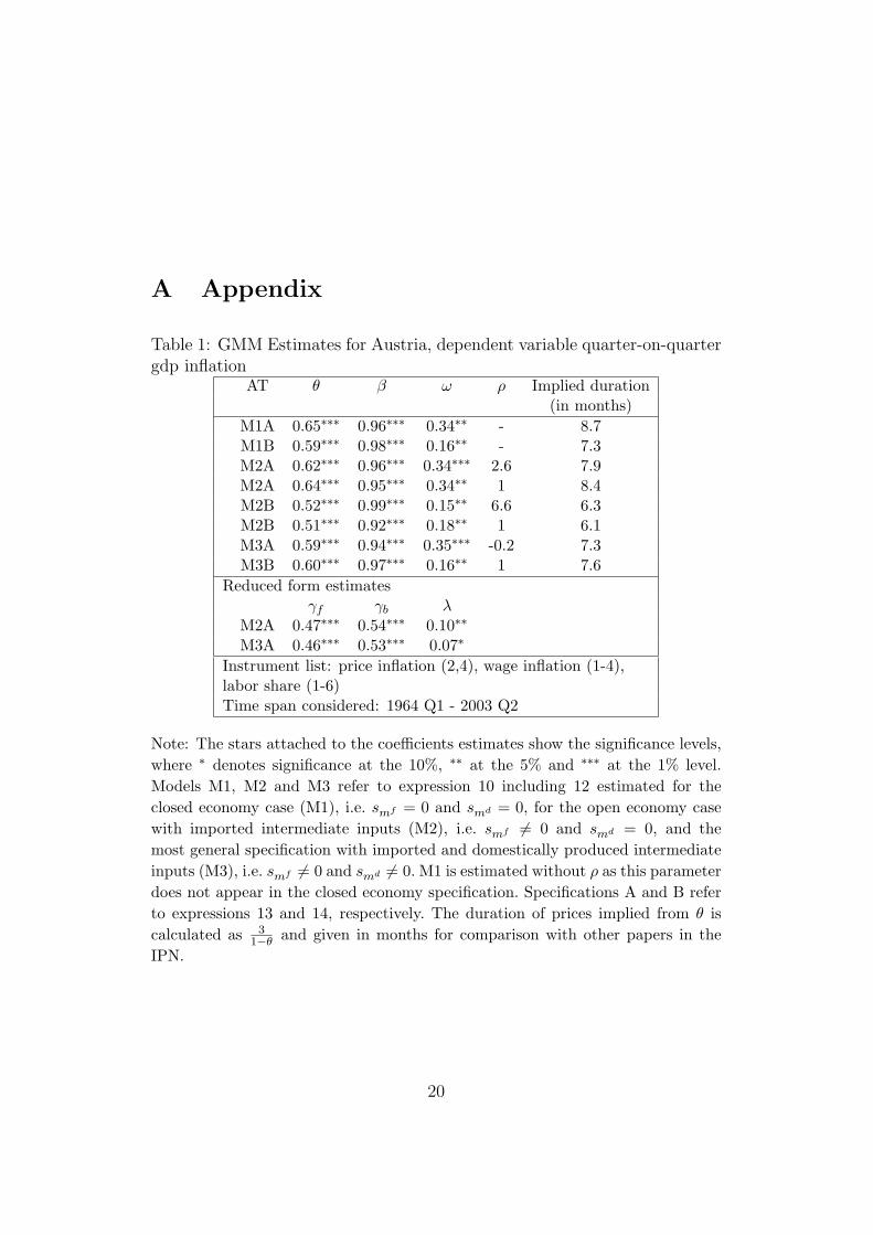
Table 1: GMM Estimates for Austria, dependent variable quarter-on-quartergdp inflation
AT θ β ω ρ Implied duration(in months)
M1A 0.65∗∗∗ 0.96∗∗∗ 0.34∗∗ - 8.7M1B 0.59∗∗∗ 0.98∗∗∗ 0.16∗∗ - 7.3M2A 0.62∗∗∗ 0.96∗∗∗ 0.34∗∗∗ 2.6 7.9M2A 0.64∗∗∗ 0.95∗∗∗ 0.34∗∗ 1 8.4M2B 0.52∗∗∗ 0.99∗∗∗ 0.15∗∗ 6.6 6.3M2B 0.51∗∗∗ 0.92∗∗∗ 0.18∗∗ 1 6.1M3A 0.59∗∗∗ 0.94∗∗∗ 0.35∗∗∗ -0.2 7.3M3B 0.60∗∗∗ 0.97∗∗∗ 0.16∗∗ 1 7.6
Reduced form estimatesγf γb λ
M2A 0.47∗∗∗ 0.54∗∗∗ 0.10∗∗
M3A 0.46∗∗∗ 0.53∗∗∗ 0.07∗
Instrument list: price inflation (2,4), wage inflation (1-4),labor share (1-6)Time span considered: 1964 Q1 - 2003 Q2
Note: The stars attached to the coefficients estimates show the significance levels,where ∗ denotes significance at the 10%, ∗∗ at the 5% and ∗∗∗ at the 1% level.Models M1, M2 and M3 refer to expression 10 including 12 estimated for theclosed economy case (M1), i.e. smf = 0 and smd = 0, for the open economy casewith imported intermediate inputs (M2), i.e. smf 6= 0 and smd = 0, and themost general specification with imported and domestically produced intermediateinputs (M3), i.e. smf 6= 0 and smd 6= 0. M1 is estimated without ρ as this parameterdoes not appear in the closed economy specification. Specifications A and B referto expressions 13 and 14, respectively. The duration of prices implied from θ iscalculated as 3
1−θ and given in months for comparison with other papers in theIPN.
20
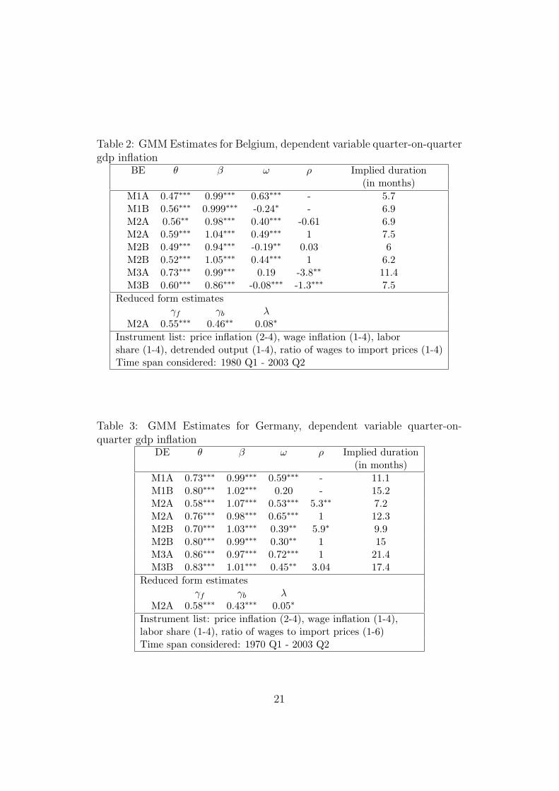
Table 2: GMM Estimates for Belgium, dependent variable quarter-on-quartergdp inflation
BE θ β ω ρ Implied duration(in months)
M1A 0.47∗∗∗ 0.99∗∗∗ 0.63∗∗∗ - 5.7M1B 0.56∗∗∗ 0.999∗∗∗ -0.24∗ - 6.9M2A 0.56∗∗ 0.98∗∗∗ 0.40∗∗∗ -0.61 6.9M2A 0.59∗∗∗ 1.04∗∗∗ 0.49∗∗∗ 1 7.5M2B 0.49∗∗∗ 0.94∗∗∗ -0.19∗∗ 0.03 6M2B 0.52∗∗∗ 1.05∗∗∗ 0.44∗∗∗ 1 6.2M3A 0.73∗∗∗ 0.99∗∗∗ 0.19 -3.8∗∗ 11.4M3B 0.60∗∗∗ 0.86∗∗∗ -0.08∗∗∗ -1.3∗∗∗ 7.5
Reduced form estimatesγf γb λ
M2A 0.55∗∗∗ 0.46∗∗ 0.08∗
Instrument list: price inflation (2-4), wage inflation (1-4), laborshare (1-4), detrended output (1-4), ratio of wages to import prices (1-4)Time span considered: 1980 Q1 - 2003 Q2
Table 3: GMM Estimates for Germany, dependent variable quarter-on-quarter gdp inflation
DE θ β ω ρ Implied duration(in months)
M1A 0.73∗∗∗ 0.99∗∗∗ 0.59∗∗∗ - 11.1M1B 0.80∗∗∗ 1.02∗∗∗ 0.20 - 15.2M2A 0.58∗∗∗ 1.07∗∗∗ 0.53∗∗∗ 5.3∗∗ 7.2M2A 0.76∗∗∗ 0.98∗∗∗ 0.65∗∗∗ 1 12.3M2B 0.70∗∗∗ 1.03∗∗∗ 0.39∗∗ 5.9∗ 9.9M2B 0.80∗∗∗ 0.99∗∗∗ 0.30∗∗ 1 15M3A 0.86∗∗∗ 0.97∗∗∗ 0.72∗∗∗ 1 21.4M3B 0.83∗∗∗ 1.01∗∗∗ 0.45∗∗ 3.04 17.4
Reduced form estimatesγf γb λ
M2A 0.58∗∗∗ 0.43∗∗∗ 0.05∗
Instrument list: price inflation (2-4), wage inflation (1-4),labor share (1-4), ratio of wages to import prices (1-6)Time span considered: 1970 Q1 - 2003 Q2
21
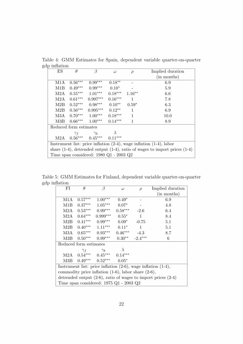
Table 4: GMM Estimates for Spain, dependent variable quarter-on-quartergdp inflation
ES θ β ω ρ Implied duration(in months)
M1A 0.56∗∗∗ 0.99∗∗∗ 0.18∗∗ - 6.9M1B 0.49∗∗∗ 0.99∗∗∗ 0.10∗ - 5.9M2A 0.55∗∗∗ 1.01∗∗∗ 0.18∗∗∗ 1.16∗∗ 6.6M2A 0.61∗∗∗ 0.997∗∗∗ 0.16∗∗∗ 1 7.8M2B 0.52∗∗∗ 0.98∗∗∗ 0.10∗∗ 0.59∗ 6.3M2B 0.56∗∗∗ 0.995∗∗∗ 0.12∗∗ 1 6.9M3A 0.70∗∗∗ 1.00∗∗∗ 0.18∗∗∗ 1 10.0M3B 0.66∗∗∗ 1.00∗∗∗ 0.14∗∗∗ 1 8.9
Reduced form estimatesγf γb λ
M2A 0.56∗∗∗ 0.45∗∗∗ 0.11∗∗∗
Instrument list: price inflation (2-4), wage inflation (1-4), laborshare (1-4), detrended output (1-4), ratio of wages to import prices (1-4)Time span considered: 1980 Q1 - 2003 Q2
Table 5: GMM Estimates for Finland, dependent variable quarter-on-quartergdp inflation
FI θ β ω ρ Implied duration(in months)
M1A 0.57∗∗∗ 1.00∗∗∗ 0.49∗ - 6.9M1B 0.37∗∗∗ 1.05∗∗∗ 0.07∗ - 4.8M2A 0.53∗∗∗ 0.99∗∗∗ 0.58∗∗∗ -2.6 6.4M2A 0.64∗∗∗ 0.999∗∗∗ 0.55∗ 1 8.4M2B 0.41∗∗∗ 0.99∗∗∗ 0.09∗ -0.75 5.1M2B 0.40∗∗∗ 1.11∗∗∗ 0.11∗ 1 5.1M3A 0.65∗∗∗ 0.93∗∗∗ 0.46∗∗∗ -4.3 8.7M3B 0.50∗∗∗ 0.99∗∗∗ 0.30∗∗ -2.4∗∗∗ 6
Reduced form estimatesγf γb λ
M2A 0.54∗∗∗ 0.45∗∗∗ 0.14∗∗∗
M3B 0.49∗∗∗ 0.52∗∗∗ 0.05∗
Instrument list: price inflation (2-6), wage inflation (1-4),commodity price inflation (1-6), labor share (2-6),detrended output (2-6), ratio of wages to import prices (2-4)Time span considered: 1975 Q1 - 2003 Q2
22

Table 6: GMM Estimates for France, dependent variable quarter-on-quartergdp inflation
FR θ β ω ρ Implied duration(in months)
M1A 0.71∗∗∗ 0.99∗∗∗ 0.57∗∗ - 10.3M1B 0.32∗∗ 1.15∗∗∗ 0.16∗∗∗ - 4.5M2A 0.65∗∗∗ 0.99∗∗∗ 0.48∗∗∗ 2.6 8.7M2A 0.65∗∗∗ 0.99∗∗∗ 0.51∗∗∗ 1 8.7M2B 0.50∗∗∗ 0.98∗∗∗ 0.10∗∗ 1.9∗∗∗ 6M2B 0.50∗∗∗ 1.00∗∗∗ 0.12∗∗∗ 1 6M3A 0.71∗∗∗ 0.94∗∗∗ 0.56∗∗∗ -4.3 10.5M3B 0.62∗∗∗ 0.975∗∗∗ 0.13∗∗ -0.6 7.8
Reduced form estimatesγf γb λ
M2A 0.63∗∗∗ 0.40∗∗∗ 0.33∗∗∗
Instrument list: price inflation (2-4), wage inflation (1-4),commodity price inflation (1-4), labor share (1-4),detrended output (1-4), ratio of wages to import prices (1-6)Time span considered: 1978 Q1 - 2003 Q2
23
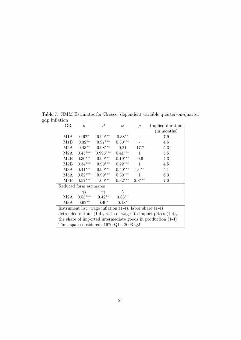
Table 7: GMM Estimates for Greece, dependent variable quarter-on-quartergdp inflation
GR θ β ω ρ Implied duration(in months)
M1A 0.62∗ 0.99∗∗∗ 0.38∗∗ - 7.9M1B 0.32∗∗ 0.97∗∗∗ 0.30∗∗∗ - 4.5M2A 0.43∗∗ 0.98∗∗∗ 0.21 -17.7 5.3M2A 0.45∗∗∗ 0.995∗∗∗ 0.41∗∗∗ 1 5.5M2B 0.30∗∗∗ 0.99∗∗∗ 0.19∗∗∗ -0.6 4.3M2B 0.34∗∗∗ 0.99∗∗∗ 0.22∗∗∗ 1 4.5M3A 0.41∗∗∗ 0.99∗∗∗ 0.40∗∗∗ 1.6∗∗ 5.1M3A 0.52∗∗∗ 0.99∗∗∗ 0.39∗∗∗ 1 6.3M3B 0.57∗∗∗ 1.00∗∗∗ 0.32∗∗∗ 2.8∗∗∗ 7.0
Reduced form estimatesγf γb λ
M2A 0.55∗∗∗ 0.42∗∗ 3.83∗∗
M3A 0.62∗∗ 0.40∗ 0.18∗
Instrument list: wage inflation (1-4), labor share (1-4)detrended output (1-4), ratio of wages to import prices (1-4),the share of imported intermediate goods in production (1-4)Time span considered: 1970 Q1 - 2003 Q2
24
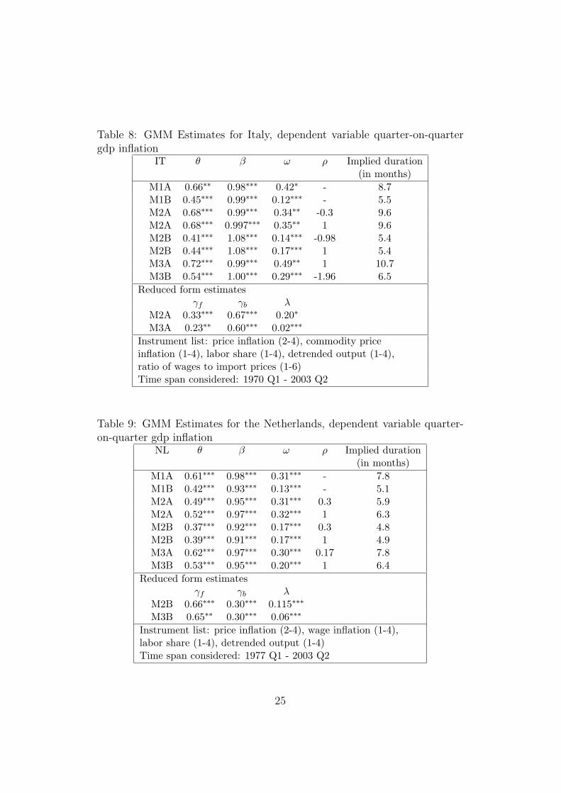
Table 8: GMM Estimates for Italy, dependent variable quarter-on-quartergdp inflation
IT θ β ω ρ Implied duration(in months)
M1A 0.66∗∗ 0.98∗∗∗ 0.42∗ - 8.7M1B 0.45∗∗∗ 0.99∗∗∗ 0.12∗∗∗ - 5.5M2A 0.68∗∗∗ 0.99∗∗∗ 0.34∗∗ -0.3 9.6M2A 0.68∗∗∗ 0.997∗∗∗ 0.35∗∗ 1 9.6M2B 0.41∗∗∗ 1.08∗∗∗ 0.14∗∗∗ -0.98 5.4M2B 0.44∗∗∗ 1.08∗∗∗ 0.17∗∗∗ 1 5.4M3A 0.72∗∗∗ 0.99∗∗∗ 0.49∗∗ 1 10.7M3B 0.54∗∗∗ 1.00∗∗∗ 0.29∗∗∗ -1.96 6.5
Reduced form estimatesγf γb λ
M2A 0.33∗∗∗ 0.67∗∗∗ 0.20∗
M3A 0.23∗∗ 0.60∗∗∗ 0.02∗∗∗
Instrument list: price inflation (2-4), commodity priceinflation (1-4), labor share (1-4), detrended output (1-4),ratio of wages to import prices (1-6)Time span considered: 1970 Q1 - 2003 Q2
Table 9: GMM Estimates for the Netherlands, dependent variable quarter-on-quarter gdp inflation
NL θ β ω ρ Implied duration(in months)
M1A 0.61∗∗∗ 0.98∗∗∗ 0.31∗∗∗ - 7.8M1B 0.42∗∗∗ 0.93∗∗∗ 0.13∗∗∗ - 5.1M2A 0.49∗∗∗ 0.95∗∗∗ 0.31∗∗∗ 0.3 5.9M2A 0.52∗∗∗ 0.97∗∗∗ 0.32∗∗∗ 1 6.3M2B 0.37∗∗∗ 0.92∗∗∗ 0.17∗∗∗ 0.3 4.8M2B 0.39∗∗∗ 0.91∗∗∗ 0.17∗∗∗ 1 4.9M3A 0.62∗∗∗ 0.97∗∗∗ 0.30∗∗∗ 0.17 7.8M3B 0.53∗∗∗ 0.95∗∗∗ 0.20∗∗∗ 1 6.4
Reduced form estimatesγf γb λ
M2B 0.66∗∗∗ 0.30∗∗∗ 0.115∗∗∗
M3B 0.65∗∗ 0.30∗∗∗ 0.06∗∗∗
Instrument list: price inflation (2-4), wage inflation (1-4),labor share (1-4), detrended output (1-4)Time span considered: 1977 Q1 - 2003 Q2
25

Table 10: GMM Estimates for the Euro Area, dependent variable quarter-on-quarter gdp inflation
EA θ β ω ρ Implied duration(in months)
M1A 0.78∗∗∗ 1.02∗∗∗ 0.48∗∗∗ - 13.6M1B 0.59∗∗∗ 0.99∗∗∗ 0.37∗∗∗ - 7.3M2A 0.67∗∗∗ 1.02∗∗∗ 0.50∗∗∗ 5.7 9.1M2A 0.68∗∗∗ 1.02∗∗∗ 0.50∗∗∗ 1 9.6M2B 0.51∗∗∗ 0.999∗∗∗ 0.19∗∗ 0.41 6.1M2B 0.51∗∗∗ 1.00∗∗∗ 0.21∗∗∗ 1 6.1M3A 0.64∗∗∗ 1.03∗∗∗ 0.44∗∗∗ 1 8.4M3B 0.52∗∗∗ 1.02∗∗∗ 0.20∗ 1.01∗ 6.3
Reduced form estimatesγf γb λ
M2A 0.29∗∗∗ 0.72∗∗∗ 0.11∗∗∗
M3A 0.52∗∗∗ 0.49∗∗∗ 0.09∗∗∗
Instrument list: price inflation (2-4), wage inflation (1-4),commodity price inflation (1-4), labor share (1-6),ratio of wages to import prices (1-4)Time span considered: 1970 Q1 - 1998 Q4
26
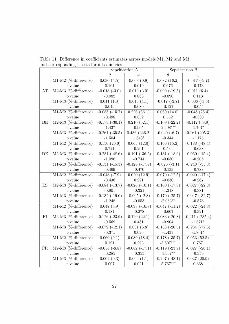
Table 11: Difference in coefficients estimates across models M1, M2 and M3and corresponding t-tests for all countries
Sepcification A Sepcification Bθ ω θ ω
M1-M2 (%-difference) 0.030 (5.5) 0.003 (0.9) 0.082 (16.2) -0.017 (-9.7)t-value 0.161 0.019 0.676 -0.173
AT M2-M3 (%-difference) -0.018 (-3.0) 0.010 (3.0) -0.099 (-19.5) 0.011 (6.4)t-value -0.082 0.063 -0.890 0.113
M1-M3 (%-difference) 0.011 (1.8) 0.013 (4.1) -0.017 (-2.7) -0.006 (-3.5)t-value 0.049 0.080 -0.127 -0.054
M1-M2 (%-difference) -0.088 (-15.7) 0.226 (56.1) 0.069 (14.0) -0.048 (25.4)t-value -0.498 0.852 0.552 -0.330
BE M2-M3 (%-difference) -0.173 (-30.1) 0.210 (52.1) -0.109 (-22.2) -0.112 (58.9)t-value -1.437 0.905 -2.498∗∗∗ -1.707∗
M1-M3 (%-difference) -0.261 (-35.5) 0.436 (226.2) -0.040 (-6.7) -0.161 (205.3)t-value -1.504 1.643∗ -0.344 -1.175
M1-M2 (%-difference) 0.150 (26.0) 0.063 (12.0) 0.106 (15.2) -0.188 (-48.4)t-value 0.721 0.291 0.534 -0.638
DE M2-M3 (%-difference) -0.281 (-48.6) -0.191 (-36.2) -0.131 (-18.9) -0.060 (-15.4)t-value -1.096 -0.744 -0.650 -0.205
M1-M3 (%-difference) -0.131 (-15.3) -0.128 (-17.8) -0.026 (-3.1) -0.248 (-55.3)t-value -0.469 -0.470 -0.133 -0.788
M1-M2 (%-difference) -0.048 (-7.9) 0.020 (12.9) -0.070 (-12.5) -0.020 (-17.4)t-value -0.436 0.221 -0.830 -0.267
ES M2-M3 (%-difference) -0.084 (-13.7) -0.026 (-16.1) -0.100 (-17.8) -0.027 (-22.8)t-value -0.901 -0.321 -1.318 -0.381
M1-M3 (%-difference) -0.132 (-19.0) -0.005 (-2.8) -0.170 (-25.7) -0.047 (-32.7)t-value -1.248 -0.053 -2.063∗∗ -0.578
M1-M2 (%-difference) 0.047 (8.9) -0.098 (-16.8) -0.047 (-11.2) -0.022 (-24.8)t-value 0.187 -0.278 -0.607 -0.321
FI M2-M3 (%-difference) -0.126 (-23.9) 0.129 (22.1) -0.083 (-20.8) -0.211 (-235.4)t-value -0.569 0.481 -0.904 -1.571∗
M1-M3 (%-difference) -0.079 (-12.1) 0.031 (6.8) -0.133 (-26.5) -0.234 (-77.6)t-value -0.371 0.096 -1.433 -1.801∗
M1-M2 (%-difference) 0.060 (9.1) 0.089 (18.4) -0.178 (-35.7) 0.053 (52.5)t-value 0.191 0.293 -3.607∗∗∗ 0.767
FR M2-M3 (%-difference) -0.058 (-8.8) -0.082 (-17.1) -0.119 (-23.9) -0.027 (-26.1)t-value -0.285 -0.355 -1.997∗∗ -0.359
M1-M3 (%-difference) 0.002 (0.3) 0.006 (1.1) -0.297 (-48.1) 0.027 (20.9)t-value 0.007 0.021 -5.767∗∗∗ 0.368
27
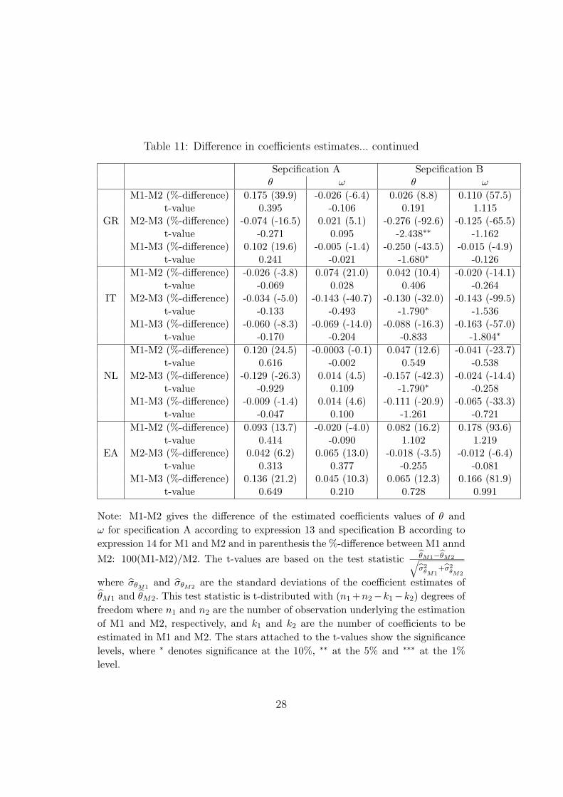
Table 11: Difference in coefficients estimates... continued
Sepcification A Sepcification Bθ ω θ ω
M1-M2 (%-difference) 0.175 (39.9) -0.026 (-6.4) 0.026 (8.8) 0.110 (57.5)t-value 0.395 -0.106 0.191 1.115
GR M2-M3 (%-difference) -0.074 (-16.5) 0.021 (5.1) -0.276 (-92.6) -0.125 (-65.5)t-value -0.271 0.095 -2.438∗∗ -1.162
M1-M3 (%-difference) 0.102 (19.6) -0.005 (-1.4) -0.250 (-43.5) -0.015 (-4.9)t-value 0.241 -0.021 -1.680∗ -0.126
M1-M2 (%-difference) -0.026 (-3.8) 0.074 (21.0) 0.042 (10.4) -0.020 (-14.1)t-value -0.069 0.028 0.406 -0.264
IT M2-M3 (%-difference) -0.034 (-5.0) -0.143 (-40.7) -0.130 (-32.0) -0.143 (-99.5)t-value -0.133 -0.493 -1.790∗ -1.536
M1-M3 (%-difference) -0.060 (-8.3) -0.069 (-14.0) -0.088 (-16.3) -0.163 (-57.0)t-value -0.170 -0.204 -0.833 -1.804∗
M1-M2 (%-difference) 0.120 (24.5) -0.0003 (-0.1) 0.047 (12.6) -0.041 (-23.7)t-value 0.616 -0.002 0.549 -0.538
NL M2-M3 (%-difference) -0.129 (-26.3) 0.014 (4.5) -0.157 (-42.3) -0.024 (-14.4)t-value -0.929 0.109 -1.790∗ -0.258
M1-M3 (%-difference) -0.009 (-1.4) 0.014 (4.6) -0.111 (-20.9) -0.065 (-33.3)t-value -0.047 0.100 -1.261 -0.721
M1-M2 (%-difference) 0.093 (13.7) -0.020 (-4.0) 0.082 (16.2) 0.178 (93.6)t-value 0.414 -0.090 1.102 1.219
EA M2-M3 (%-difference) 0.042 (6.2) 0.065 (13.0) -0.018 (-3.5) -0.012 (-6.4)t-value 0.313 0.377 -0.255 -0.081
M1-M3 (%-difference) 0.136 (21.2) 0.045 (10.3) 0.065 (12.3) 0.166 (81.9)t-value 0.649 0.210 0.728 0.991
Note: M1-M2 gives the difference of the estimated coefficients values of θ andω for specification A according to expression 13 and specification B according toexpression 14 for M1 and M2 and in parenthesis the %-difference between M1 anndM2: 100(M1-M2)/M2. The t-values are based on the test statistic θM1−θM2√
σ2θM1
+σ2θM2
where σθM1and σθM2
are the standard deviations of the coefficient estimates ofθM1 and θM2. This test statistic is t-distributed with (n1 +n2−k1−k2) degrees offreedom where n1 and n2 are the number of observation underlying the estimationof M1 and M2, respectively, and k1 and k2 are the number of coefficients to beestimated in M1 and M2. The stars attached to the t-values show the significancelevels, where ∗ denotes significance at the 10%, ∗∗ at the 5% and ∗∗∗ at the 1%level.
28