SFB 649 Discussion Paper 2010-030

Can the New Keynesian Phillips Curve Explain

Inflation Gap Persistence?

Fang Yao*

* Humboldt Universität zu Berlin, Germany

This research was supported by the Deutsche Forschungsgemeinschaft through the SFB 649 "Economic Risk".

http://sfb649.wiwi.hu-berlin.de

ISSN 1860-5664

SFB 649, Humboldt-Universität zu Berlin Spandauer Straße 1, D-10178 Berlin

SFB

6

4 9

E

C O

N O

M I

C

R

I S

K

B

E R

L I

N

Can the New Keynesian Phillips Curve Explain In�ation GapPersistence?

Fang Yao�

Humboldt Universität zu Berlin

May 27, 2010

Abstract

Whelan (2007) found that the generalized Calvo-sticky-price model fails to replicate atypical feature of the empirical reduced-form Phillips curve � the positive dependence ofin�ation on its own lags. In this paper, I show that it is the 4-period-Taylor-contract hazardfunction he chose that gives rise to this result. In contrast, an empirically-based aggregateprice reset hazard function can generate simulated data that are consistent with in�ationgap persistence found in US CPI data. I conclude that a non-constant price reset hazardplays a crucial role for generating realistic in�ation dynamics.

JEL classi�cation: E12; E31Key words: In�ation gap persistence, Trend in�ation, New Keynesian Phillips curve,

Hazard function

�I am grateful to Michael Burda, Alexander Meyer-Gohde, Lutz Weinke and other seminar participants inBerlin for helpful comments. I acknowledge the support of the Deutsche Bundesbank and the Deutsche Forschungs-gemeinschaft through the CRC 649 "Economic Risk". All errors are my sole responsibility. Address: Institutefor Economic Theory, Humboldt University of Berlin, Spandauer Str. 1, Berlin, Germany +493020935667, email:yaofang@rz.hu-berlin.de.

1

Contents

1 Introduction 2

2 In�ation Persistence in the Data 4

3 The Model 73.1 Representative Household . . . . . . . . . . . . . . . . . . . . . . . . . . . . . . . 73.2 Firms in the Economy . . . . . . . . . . . . . . . . . . . . . . . . . . . . . . . . . 8

3.2.1 Real Marginal Cost . . . . . . . . . . . . . . . . . . . . . . . . . . . . . . . 83.2.2 Pricing Decisions under Nominal Rigidity . . . . . . . . . . . . . . . . . . 8

4 New Keynesian Phillips Curve 104.1 Economic Intuition . . . . . . . . . . . . . . . . . . . . . . . . . . . . . . . . . . . 114.2 Implications for in�ation gap persistence . . . . . . . . . . . . . . . . . . . . . . . 134.3 The General Equilibrium Analysis . . . . . . . . . . . . . . . . . . . . . . . . . . 14

4.3.1 Calibration . . . . . . . . . . . . . . . . . . . . . . . . . . . . . . . . . . . 154.3.2 Numerical Results . . . . . . . . . . . . . . . . . . . . . . . . . . . . . . . 16

5 Conclusion 18

A Deviation of the New Keynesian Phillips Curve 21

B Proof 24

1

1 Introduction

The nature of in�ation persistence is a complex phenomenon, because it is in�uenced by manyaspects of the economy. For example, Cogley and Sbordone (2008) argue that it is important todistinguish between the in�ation trend persistence and the in�ation gap persistence, since theyarise from di¤erent economic sources. While dynamics of trend in�ation results largely fromshifts in the long-run target of the monetary policy rule, in�ation gap persistence is in�uencedprimarily by the pricing behavior at the �rm�s level and the price aggregation mechanism.

The focus of this paper is the dynamics of the in�ation gap � the di¤erence between theactual in�ation and trend in�ation. I �rst document some stylized facts distinguishing in�ationgap persistence from in�ation level persistence. I �nd evidence from the U.S. CPI data thatthe in�ation gap constitutes a large part of in�ation persistence. Second, I investigate whetherthe stylized fact can be explained by the theoretical New Keynesian Phillips curve ( hereafter:NKPC), and further identify which mechanism of the model is most important for generatingin�ation gap persistence.

The purely forward-looking NKPC is often criticized for generating too little in�ation persis-tence (See: e.g. Fuhrer and Moore, 1995). To overcome this weakness, various generalizations ofthe basic NKPC have been developed in the literature, they o¤er, however, di¤erent interpreta-tions on the nature of in�ation gap persistence. The hybrid NKPC incorporates lagged in�ationinto the standard NKPC motivated by the positive backward-dependence of in�ation in theempirical reduced-form Phillips curve1. According to this line of literature, in�ation gap per-sistence should be interpreted as �intrinsic�(Fuhrer, 2006) and the dependency between currentand lagged in�ation should be treated as a �xed primitive relationship, which is independentof monetary policy. By contrast, the more micro-founded general-pricing-hazard models2 shednew lights on the important role played by inertia of expectations in generating in�ation gappersistence. According to this class of models, in�ation gap persistence is inherited. It comesfrom the additional moving-average terms of real driving forces through the lagged expectations.More importantly, since the coe¢ cient on lagged in�ation depends on the whole model includingthe speci�cation of monetary policy, it implies that the hybrid NKPC should be subject to theLucas critique (Lucas, 1972), and thereby can not be used in the monetary policy analysis.

Despite the theoretical solidity of the general-pricing-hazard model, Whelan (2007) rejectedit empirically. He showed that the general-pricing-hazard model fails to replicate the positivebackward-dependence of in�ation typically found in the empirical reduced-form Phillips curve. Inpartial equilibrium,Whelan proved that the coe¢ cient on the lagged in�ation is always negative,regardless of the form of the price reset hazard function. Furthermore, he used a simple DSGEmodel to show that, even in general equilibrium, this model still generates negative coe¢ cientson in�ation lags.

In this paper, I �rst replicate his �ndings and check their robustness to alternative setups ofthe model. In particular, I test the result using di¤erent price reset hazard functions, aggregatedemand conditions and monetary policy rules. I �nd that it is the 4-period-Taylor-contracthazard function used in the Whelan�s setup that gave rise to the result. Under an empiricallybased pricing hazard function estimated by Yao (2010), the simulated data accounts quite well

1See: e.g. Gali and Gertler (1999) and Christiano et al. (2005).2See: e.g. Carvalho (2006), Sheedy (2007), Coenen et al. (2007) and Whelan (2007).

2

for the in�ation gap persistence I �nd in the U.S. CPI data after the Volcker disin�ation period.The reason why the hazard function greatly a¤ects in�ation gap persistence is that backward-dependence of in�ation in the model is determined by two counteracting channels. The "front-loading channel" always weakens in�ation gap persistence, because lagged in�ation enters theNKPC with negative coe¢ cients, magnitudes of which are purely determined by the price resethazard function. By contrast, the second channel works through the expectational terms in theNKPC. In this channel, lagged in�ations have positive coe¢ cients when lagged in�ations act asleading indicator of other variables. As a result, the magnitude of the "expectation channel" isnot only a¤ected by the price reset hazard function, but also by the other general equilibriumforces, such as aggregate demand side of the economy and monetary policy. Overall, in�ationgap persistence in this framework results from a more complex propagation mechanism, in whichthe price reset hazard function exerts crucial e¤ects through various channels.

The general-pricing-hazard models have been studied in the macro literature to understandconsequences of di¤erent price reset hazard functions for macro dynamics. It is important,because, in recent years, empirical studies using detailed micro-level price data sets3 generallyreach the consensus that, instead of having economy-wide uniform price stickiness, the fre-quency of price adjustments di¤ers substantially across sections. This new evidence issues aserious challenge to the Calvo pricing assumption (Calvo, 1983). In addition, micro empiricalevidence largely rejects the constant hazard function, implied by the Calvo model (See, e.g.:Cecchetti, 1986, Alvarez, 2007 and Nakamura and Steinsson, 2008). In response to this chal-lenge, theoretical work by Wolman (1999) raised the issue that in�ation dynamics should besensitive to the hazard function underlying di¤erent pricing rules. He showed this result ina partial equilibrium analysis. Kiley (2002) compared the Calvo and Taylor staggered-pricingmodels and showed the dynamics of output following monetary shocks are both quantitativelyand qualitatively di¤erent across the two pricing speci�cations unless one assumes a substantiallevel of real rigidity in the economy. Carvalho (2006) constructed a sticky price model thatallows for heterogeneous Calvo-sticky-price sectors. He found that existence of heterogeneityin price stickiness generates large and persistent real e¤ects of monetary policy, which can bereplicated by a constant-hazard-pricing model only when it is calibrated with an unrealistic lowfrequency of price adjustments. Sheedy (2007) derived the generalized NKPC under a recursiveformulation of the hazard function and showed that, under this parameterization, the depen-dence of current and lagged in�ation is determined by the slope of the hazard function. Thisresult, however, is not applicable in more general cases. Whelan (2007) derived the NKPC undera general hazard function and showed that backward-dependence of in�ation in this structuralPhillips curve is mostly negative. Based on this �nding he drew the conclusion that this classof models can not explain the observation from the reduced-form Phillips curve regression thatin�ation is positively dependent on its lags.

It is noteworthy that non-zero trend in�ation is also important for the short-run in�ationdynamics(See: Ascari, 2004). Furthermore, Cogley and Sbordone (2008) extend the CalvoNKPC by allowing for time-drifting trend in�ation and they show that changing trend in�ationa¤ects coe¢ cients of the NKPC and hence the short-run in�ation dynamics. Even though thegeneral-hazard NKPC does not incorporate this feature, this limitation does not prohibit the

3See: e.g. Bils and Klenow (2004) and Alvarez et al. (2006) among others.

3

general-price-hazard model from standing as a useful analytical tool for in�ation dynamics.Empirical evidence shows that, while non-constant hazard function is a robust feature of thepricing behavior in the data, the time-varying trend in�ation is not always equally importantall the time. During the oil crises in the 1970�s, volatile in�ation trend maybe predominatedin�ation dynamics, but, after early 1980�s, U.S. trend in�ation became moderate and stable inthe data. These two versions of the generalized NKPC complement each other, combining them,however, gives an interesting perspective for future work.

The remainder of the paper is organized as follows: Section 1 documents stylized fact ofin�ation gap persistence in the U.S. data. In section 2, I present the model with the generalizedtime-dependent pricing and derive the New Keynesian Phillips curve; section 3 shows analyticalresults regarding new insights gained from relaxing the constant hazard function underlying theCalvo assumption and implications for in�ation gap persistence is also discussed; in section 4,I simulate the DSGE model with di¤erent setups and identify the most important feature ingenerating in�ation gap persistence; section 5 contains some concluding remarks.

2 In�ation Persistence in the Data

Whelan (2007) has documented that U.S. in�ation in the post-WWII periods is highly persistentwhen measured by the sum of autocorrelation coe¢ cients of in�ation level and the coe¢ cientof lagged in�ation in the reduced-form Phillips curve. Based on this evidence, he rejected thegeneral-pricing hazard model as a valid model for in�ation dynamics. However, it is importantto distinguish the in�ation gap persistence from the in�ation trend persistence, because stickyprice models are really designed to explain the short-run dynamics of in�ation gap which arecaused by the collective pricing behavior of �rms in the economy, instead of the dynamics oftrend in�ation which are mainly determined by the central bank�s monetary policy targets.

Recently, there are a growing number of studies on in�ation persistence controlling a driftingtrend in�ation. Levin and Piger (2003), Altissimo et al. (2006), Cogley and Sbordone (2008)and Cogley et al. (2008) document using both U.S. and European data that, when correctlyaccounting for the time-varing trend in�ation, various measures of in�ation gap persistence fallsigni�cantly. Here I present evidence on in�ation gap persistence using the U.S. CPI data. Inaddition, I report results controlling di¤erent measures for trend in�ation.

I estimate two measures of in�ation persistence using the U.S. time series data from 1960 Q1to 2007 Q44. First, following Andrews and Chen (1992), I calculate the sum of AR coe¢ cients

4 I download data from the database FRED maintained by the Federal Reserve Bank of St. Louis. I calculate thein�ation rate by using the Consumer Price Index data for all urban consumers: all items and seasonally adjusted(Series: CPIAUCSL). The monthly data is �rst converted into quarterly frequency by arithmetic averaging andthen the annualized In�ation rate is de�ned as 400� ln (Pt=Pt�1) : Furthermore, to measure the real in�ationarypressures, I �rst construct data of real output gap per capita, which is based on the Real GDP (Series: GDPC1).They are in the unit of billions of chained 2005 dollars, quarterly frequency and seasonally adjusted. To calculatereal GDP per capita, I use the Civilian Noninstitutional Population (Series: CNP16OV) from the Bureau of LaborStatistics. The monthly data in the unit of thousands is �rst converted into quarterly frequency by arithmeticaveraging. The real GDP per capita is de�ned as: ln (GDPt � 1; 000; 000=POPt) : Finally real output gap percapita is obtained by detrending the data by the Hodrick-Prescott �lter. In addition, I download the unit laborshare for non-farm business sector (Series: PRS85006173) from the U.S. Bureau of Labor Statistics as a measureof real marginal cost.

4

1960 1965 1970 1975 1980 1985 1990 1995 2000 2005

0

1

2

3

4

5

6

InflationTrend Inflation (C­S)Trend Inflation (H­P)

1960 1965 1970 1975 1980 1985 1990 1995 2000 2005

0.5

1

1.5

2

2.5

3

3.5

4

4.5

5Trend Inflation(C­S)Trend Inflation(H­P)5% Quantile95% Quantile

Figure 1: Measures of Trend In�ation

as a measure of overall in�ation persistence. Second, following Whelan (2007), I estimate thereduced-form Phillips curve by including real driving forces into the regression. This reduced-form in�ation regression distinguishes in�ation persistence driven by its own lags5 from thoseimparted by persistent real driving forces. The reduced-form in�ation regression is speci�ed inthe following form and I report the coe¢ cient � as the measure of in�ation persistence

�t = � + ��t�1 +3Pi=1�i��t�i +

3Pi=0�iyt�i + ut: (1)

To construct in�ation gap, we need to �rst calculate measures of the in�ation trend. Sincethere is no standard way to do it in the literature, I �rst choose a naive method to detrendin�ation by the Hodrick-Prescott (H-P) �lter. The biggest limitation of this method, however,is that the H-P �lter is only based on the univariate process. As argued by Cogley and Sbordone(2008), when the trend in�ation is nonzero and drifting over time, it should also depend on otherreal variables, such as the trend of real marginal cost. To account for this feature of the data,they proposed to estimate a VAR model with drifting parameters and stochastic volatility forfour variables - output growth rate, the log of unit labor cost, in�ation and the nominal discountfactor. After that, they calculate an approximation of trend in�ation by de�ning it as the level towhich in�ation expectation settles in the long run. Following the same methodology, I constructCPI in�ation trend for the periods between 1960 Q1 to 2007 Q46.

In Figure (1), I plot the two measures of trend in�ation. In the left panel, we observe thatthe two trends di¤er substantially. While the H-P trend (dashed line) follows closely to actualin�ation, the Cogley-Sbordone trend (hereafter: C-S trend) is much more moderate. The medianestimate of trend in�ation rose by roughly 1% at the annual rate during 1970�s and fell backto around 1.3% in the early 80�s, then stayed relative stable until 2007. On the right panel, I

5 It is denoted as the intrinsic in�ation persistence by some authers, e.g.: Sheedy (2007)6For calculating this in�ation trend, I implement the MATLAB codes provided by Timothy Cogley and Argia

M. Sbordone on their website.

5

compare the two trends more closely. As portrayed by the two dash lines, the 90% con�dentinterval of estimated C-S in�ation trend is quite wide, especially during the volatile periods in1970�s. It indicates a great deal of uncertainty about trend in�ation associating with the C-Smethod. Even through the H-P trend is substantially di¤erent to the C-S trend, it lies withinthe con�dent interval for the most of sample periods. Due to this reason, in Table (1), I reportmeasures of in�ation gap persistence for both H-P and C-S trend in�ation.

In�ation level In�ation Gap (H-P) In�ation Gap (C-S)

Sample AR �(y) �(LS) AR �(y) �(LS) AR �(y) �(LS)

1960� 2007 0:887(0:041)

0:897(0:041)

0:882(0:046)

0:559(0:082)

0:479(0:095)

0:548(0:084)

0:825(0:051)

0:849(0:053)

0:807(0:055)

1960� 1985 0:902(0:048)

0:895(0:047)

0:906(0:051)

0:659(0:094)

0:574(0:109)

0:642(0:103)

0:858(0:056)

0:873(0:058)

0:850(0:063)

1986� 2007 0:491(0:145)

0:494(0:155)

0:475(0:153)

0:064(0:185)

0:013(0:200)

0:062(0:187)

0:376(0:16)

0:364(0:172)

0:378(0:165)

Note: Numbers in the parenthesis are the standard deviations.

Table 1: Empirical Results based on the In�ation Data

The �rst row of the table indicates which de�nition of in�ation is used to calculate themeasures of persistence. I report results for in�ation level, in�ation gap detrended by the H-P�lter and in�ation gap detrended by the Cogley and Sbordone method. Under each label, threemeasures of in�ation persistence are presented, i.e. the sum of autocorrelation coe¢ cients AR,the coe¢ cient of lagged in�ation in the reduced-form Phillips curve when the real driving forceis measured by H-P detrended real output per capita �(y), and the coe¢ cient of lagged in�ationin the reduced-form Phillips curve when the real driving force is measured by the unit laborshare �(LS). The �rst noteworthy result from the table is that the CPI in�ation was indeedhighly persistent over the subsample from 1960 to 1985. It fell dramatically, however, after theVolcker disin�ation of 1980�s. This �nding is consistent with what is found in the literature.Second, the magnitude of in�ation gap persistence crucially depends on the measure of trendin�ation. When the H-P trend is used, in�ation gap persistence is signi�cantly lower than thatin the in�ation level. It becomes even insigni�cant from zero during the second subsample. Bycontrast, when the C-S trend is used, in�ation gap persistence is lower, but much closer to themeasured in�ation level persistence. It is instructive to compare the C-S trend with two extremecases of in�ation detrending, namely the linear detrending and the detrending by the H-P �lter.While the mean detrending does not change the in�ation persistence at all, the H-P detrendingreduces it to the greatest extent. The multivariable-based C-S method gives values betweenthese two extreme cases. Even through it is not very accurate, one can still draw conclusionfrom this evidence that the true in�ation gap persistence is signi�cant and positive and in�ationgap persistence constitutes a large part of in�ation persistence. In the later section, I will usethe C-S measure of in�ation gap persistence as the benchmark for evaluating the performanceof the theoretical model.

In the light of these results, we can sum up some stylized facts of in�ation gap persistence.1. In�ation gap persistence constitutes a large part of in�ation persistence in the U.S. CPI data.2. CPI in�ation gap is highly persistent during periods between 1960 to 1985. The sum ofcoe¢ cients on lagged in�ation lies in the range around 0:85 with the standard deviation of 0:06.

6

3. in�ation gap persistence reduces signi�cantly after the Volcker disin�ation period. The sumof coe¢ cients on lagged in�ation reduces to around 0:37 with the standard deviation of 0:16.

3 The Model

In this section, I use a DSGE model to analyze the persistence of in�ation gap found in theU.S. data. The main feature of the model is the incorporation of a general price reset hazardfunction into an otherwise standard New Keynesian model. A hazard function of price settingis de�ned as the probabilities of price adjustment conditional on the spell of time elapsed sincethe last price change. In this model, the hazard function is a discrete function taking valuesbetween zero and one on its time domain.

3.1 Representative Household

A representative, in�nitely-lived household derives utility from the composite consumption goodCt, and its labor supply Lt, and it maximizes a discounted sum of utility of the form:

maxfCt;Lt;Btg

E0

" 1Xt=0

�t

C1��t

1� � � �HL1+�t

1 + �

!#:

Here Ct denotes an index of the household�s consumption of each of the individual goods, Ct(i);following a constant-elasticity-of-substitution aggregator (Dixit and Stiglitz, 1977).

Ct ��Z 1

0Ct(i)

��1� di

� ���1

; (2)

where � > 1, and it follows that the corresponding cost-minimizing demand for Ct(i) and thewelfare-based price index, Pt; are given by

Ct(i) =

�Pt(i)

Pt

���Ct (3)

Pt =

�Z 1

0Pt(i)

1��di

� 11��

: (4)

For simplicity, I assume that households supply homogeneous labor units (Lt) in an economy-wide competitive labor market.

The �ow budget constraint of the household at the beginning of period t is

PtCt +BtRt�WtLt +Bt�1 +

Z 1

0�t(i)di: (5)

Where Bt is a one-period nominal bond and Rt denotes the gross nominal return on the bond.�t(i) represents the nominal pro�ts of a �rm that sells good i. I assume that each household ownsan equal share of all �rms. Finally this sequence of period budget constraints is supplementedwith a transversality condition of the form lim

T!1Et

hBT

�Ts=1Rs

i> 0.

The solution to the household�s optimization problem can be expressed in two �rst ordernecessary conditions. First, optimal labor supply is related to the real wage:

7

�HL�t C

�t =

Wt

Pt: (6)

Second, the Euler equation gives the relationship between the optimal consumption path andasset prices:

1 = �Et

"�CtCt+1

��

RtPtPt+1

#: (7)

3.2 Firms in the Economy

3.2.1 Real Marginal Cost

The production side of the economy is composed of a continuum of monopolistic competitive�rms, each producing one variety of product i by using labor. Each �rm maximizes real pro�ts,subject to the production function

Yt(i) = ZtLt(i) (8)

where Zt denotes an aggregate productivity shock. Log deviations of the shock, zt; follow anexogenous AR(1) process zt = �z zt�1 + "z;t, and "z;t is white noise with �z 2 [0; 1). Lt(i) is thedemand of labor by �rm i.

Following equation (3), demand for intermediate goods is given by

Yt(i) =

�Pt(i)

Pt

���Yt: (9)

In each period, �rms choose optimal demands for labor inputs to maximize their real pro�tsgiven nominal wage, market demand (9) and the production technology (8):

maxLt(i)

�t(i) =Pt(i)

PtYt(i)�

Wt

PtLt(i) (10)

And real marginal cost can be derived from this maximization problem

mct =Wt=PtZt

:

Furthermore, using the production function (8), output demand equation (9), the labor supplycondition (6) and the fact that at the equilibrium Ct = Yt, I can express real marginal cost onlyin terms of aggregate output and technology shock.

mct = Y�+�t Z

�(1+�)t : (11)

3.2.2 Pricing Decisions under Nominal Rigidity

In this section, I introduce a general form of nominal rigidity, which is characterized by aset of hazard rates depending on the spell of the time since last price adjustment. I assumethat monopolistic competitive �rms cannot adjust their price whenever they want. Instead,opportunities for re-optimizing prices are dictated by the hazard rates, hj , where j denotes thetime-since-last-adjustment and j 2 f0; Jg. J is the maximum number of periods in which a�rm�s price can be �xed.

8

Dynamics of the Price-duration Distribution In the economy, �rms�prices are hetero-geneous with respect to the time since their last price adjustment. Table 2 summarizes keynotations concerning the dynamics of the price-duration distribution.

Duration Hazard Rate Non-adj. Rate Survival Rate Distributionj hj �j Sj �(j)

0 0 1 1 �(0)

1 h1 �1 = 1� h1 S1 = �1 �(1)...

......

......

j hj �j = 1� hj Sj =j

�i=0�i �(j)

......

......

...J hJ = 1 �J = 0 SJ = 0 �(J)

Table 2: Notations of the Dynamics of Price-vintage-distribution.

Using the notation de�ned in Table 2, and also denoting the distribution of price durationsat the beginning of each period by �t = f�t(0); �t(1) � � � �t(J)g, we can derive the ex-postdistribution of �rms after price adjustments (~�t) as

~�t(j) =

8<:JPi=1hi�t(i) , when j = 0

�j�t(j) , when j = 1 � � �J:(12)

Firms reoptimizing their prices in period t are labeled with �Duration 0�, and the proportionof those �rms is given by hazard rates of all duration groups multiplied by their correspondingdensities. The �rms left in each duration group are the �rms that do not adjust their prices.When the period t is over, this ex-post distribution, ~�t; becomes the ex-ante distribution forthe new period, �t+1: All price duration groups move to the next one, because all prices age byone period.

As long as the hazard rates lie between zero and one, dynamics of the price-duration distri-bution can be viewed as a Markov process with an invariant distribution, �, and is obtained bysolving �t(j) = �t+1(j): It yields the stationary price-duration distribution �(j):

�(j) =Sj

J�1�j=0Sj

, for j = 0; 1 � � �J � 1: (13)

In a simple example, when J = 3, the stationary price-duration distribution

� =

�1

1 + �1 + �1�2;

�11 + �1 + �1�2

;�1�2

1 + �1 + �1�2

�:

I assume the economy converges to this invariant distribution fairly quickly, so that regard-less of the initial price-duration distribution, I only consider the economy with the invariantdistribution of price durations. This assumption makes aggregation problem of the economytractable.

9

The Optimal Pricing under the General Form of Nominal Rigidity Given the generalform of nominal rigidity introduced above, the only heterogeneity among �rms is the time whenthey last reset their prices, j. Firms in price duration group j share the same probability ofadjusting their prices, hj , and the distribution of �rms across durations is given by �(j).

In a given period when a �rm is allowed to reoptimize its price, the optimal price chosenshould re�ect the possibility that it will not be re-adjusted in the near future. Consequently,adjusting �rms choose optimal prices that maximize the discounted sum of real pro�ts over thetime horizon in which the new price is expected to be �xed. The probability that a new pricewill be �xed at least for j periods is given by the survival function, Sj , de�ned in Table 2.

I setup the maximization problem of an adjuster as follows:

maxP �t

EtJ�1Pj=0

SjQt;t+j

�Y dt+jjt

P �tPt+j

� TCt+jPt+j

�:

Where Et denotes the conditional expectation based on the information set in period t, andQt;t+j is the stochastic discount factor appropriate for discounting real pro�ts from t to t + j.An adjusting �rm maximizes the pro�ts subject to the demand for its intermediate good inperiod t+ j given that the �rm resets the price in period t and can be expressed as.

Y dt+jjt =

�P �tPt+j

���Yt+j :

This yields the following �rst order necessary condition for the optimal price:

P �t =�

� � 1

J�1Pj=0

SjEt[Qt;t+jYt+jP��1t+j MCt+j ]

J�1Pj=0

SjEt[Qt;t+jYt+jP��1t+j ]

; (14)

where MCt denotes the nominal marginal cost. The optimal price is equal to the markupmultiplied by a weighted sum of future marginal costs, whose weights depend on the survivalrates. In the Calvo case, where Sj = �j , this equation reduces to the Calvo optimal pricingcondition.

Finally, given the stationary distribution, �(j), aggregate price can be written as a distributedsum of all optimal prices. I de�ne the optimal price which was set j periods ago as P �t�j .Following the aggregate price index from equation (4), the aggregate price is then obtained by:

Pt =

J�1Pj=0

�(j)P �1��t�j

! 11��

: (15)

4 New Keynesian Phillips Curve

In this section, I derive the New Keynesian Phillips curve for this generalized sticky price model.To do that, I �rst log-linearize equation (14) around the �exible price steady state. The log-

10

linearized optimal price equations are obtained by

p�t = Et

"J�1Pj=0

�jS(j)

(cmct+j + pt+j)# ; (16)

where :

=

J�1Xj=0

�jS(j) and cmct = (� + �)yt � (1 + �) zt:In a similar fashion, I derive the log deviation of the aggregate price by log linearizing equation(15).

pt =J�1Pk=0

�(k) p�t�k: (17)

After some algebraic manipulations on equations (16) and (17), I obtain the New KeynesianPhillips curve as follows7

�t =J�1Pk=0

�(k)

1� �(0)Et�k

J�1Pj=0

�jS(j)

cmct+j�k + J�1P

i=1

J�1Pj=i

�jS(j)

�t+i�k

!

�J�1Pk=2

�(k)�t�k+1; where �(k) =

J�1Pj=k

S(j)

J�1Pj=1S(j)

; =J�1Pk=0

�jS(j): (18)

4.1 Economic Intuition

The general-hazard NKPC di¤ers from the standard NKPC in two aspects. First, the general-hazard NKPC has not only current and forward-looking terms but also lagged variables andlagged expectations. In addition, all coe¢ cients in the new NKPC are nonlinear functions ofprice reset hazard rates (�j = 1� hj) and the subjective discount factor �: Thereby, short-rundynamics of in�ation gap are a¤ected by both the shape and magnitude of the price reset hazardfunction. To see the dynamic structure more clearly, I write down a simple example of the NKPCwith J = 3.

7The detailed derivation of the NKPC can be found in the technical Appendix (A).

11

�t =1

(�1 + �1�2)cmct + �1

(�1 + �1�2)cmct�1 + �1�2

(�1 + �1�2)cmct�2

+1

�1 + �1�2Et

���1cmct+1 + �2�1�2

cmct+2 + ��1 + �2�1�2

�t+1 +

�2�1�2

�t+2

�+

�1�1 + �1�2

Et�1

���1cmct + �2�1�2

cmct+1 + ��1 + �2�1�2

�t +

�2�1�2

�t+1

�+

�1�2�1 + �1�2

Et�2

���1cmct�1 + �2�1�2

cmct + ��1 + �2�1�2

�t�1 +

�2�1�2

�t

�� �1�2�1 + �1�2

�t�1; (19)

where : = 1 + ��1 + �2�1�2:

Even though, from the �rst glance, the general-hazard NKPC di¤ers substantially from theCalvo NKPC, they share the same economic intuition. In fact, should the hazard function beconstant over the in�nite horizon, the general-hazard NKPC (18) reduces to the standard CalvoNKPC8:

�t =(1� �)(1� ��)

�mct + �Et�t+1 (20)

The general-hazard NKPC nests the Calvo NKPC in the sense that, under a constant hazardfunction, lagged in�ation terms exactly cancel lagged expectations, leaving only current variablesand forward-looking expectations of in�ation in the expression.

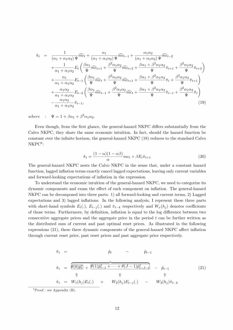
To understand the economic intuition of the general-hazard NKPC, we need to categorize itsdynamic components and exam the e¤ect of each component on in�ation. The general-hazardNKPC can be decomposed into three parts: 1) all forward-looking and current terms, 2) Laggedexpectations and 3) lagged in�ations. In the following analysis, I represent these three partswith short-hand symbols Et(:), Et�j(:) and �t�k respectively and Wx(hj) denotes coe¢ cientsof those terms. Furthermore, by de�nition, in�ation is equal to the log di¤erence between twoconsecutive aggregate prices and the aggregate price in the period t can be further written asthe distributed sum of current and past optimal reset prices. As illustrated in the followingexpressions (21), these three dynamic components of the general-hazard NKPC a¤ect in�ationthrough current reset price, past reset prices and past aggregate price respectively.

�t = pt � pt�1

�t =

z }| {�(0)p�t + �(1)p�t�1 + � � �+ �(J � 1)p�t�J�1 � pt�1 (21)

* * *�t = W1(hj)Et(:) + W2(hj)Et�j(:) � W3(hj)�t�k

8Proof : see Appendix (B).

12

The economic reasons why those three components should show up in the general-hazard NKPCis that: �rst, the current and forward-looking terms - Et(:) - enter the Phillips curve throughtheir in�uence on the current reset price. As same as in the Calvo sticky price model, the pricesetting in this model is forward-looking. The optimal price decision is based on the sum ofcurrent and future real marginal costs over the time span the reset price is �xed. The onlydi¤erence now is that the time horizon of the pricing decision is not in�nite, but depends onthe hazard function. Second, due to price stickiness, some fraction of past reset prices continueto a¤ect the current aggregate price. Lagged expectational terms -Et�j(:)- represent in�uencesof past reset prices on current in�ation. Last, past in�ations enter the NKPC, because theya¤ect the lagged aggregate price pt�1: The higher the past in�ations prevail, higher the laggedaggregate price would be, and thereby it deters current in�ation to be high.

The new insights gained from this analysis is that the two new dynamic components haveopposing e¤ects on in�ation through pt and pt�1 respectively. The magnitudes of these e¤ectsdepend on the price reset hazard function. In the general case, they should be di¤erent to eachother. Conversely, in the Calvo case, the constant hazard function leads reset prices to exertthe exactly same amount of impact on both pt and pt�1, and thereby causes lagged expectationsand lagged in�ation to be cancelled out.

This cancellation can be also seen in the derivation of the Calvo NKPC:

pt = (1� �)1Xj=0

�j p�t�j

= (1� �)�p�t + �p

�t�1 + �

2p�t�2 + � � ��

= (1� �)p�t + (1� �)��p�t�1 + �

2p�t�2 + � � ��| {z }

=�pt�1

pt = (1� �)p�t + �pt�1...

�t =(1� �)(1� ��)

�cmct + �Et(�t+1):

The crucial substitution from line (3) to line (4) is only possible, when the distribution of pricedurations takes the form of a power function. In conclusion, we learn that, lagged in�ationand lagged expectations are not extrinsic to the time-dependent sticky price model. They aremissing in the Calvo setup only because of the restrictive constant-hazard assumption.

4.2 Implications for in�ation gap persistence

The purely forward-looking NKPC is often criticized for generating too little in�ation gap per-sistence(See: e.g. Fuhrer and Moore, 1995). In response to this challenge, the hybrid NKPChas been developed to capture the positive dependence of in�ation on its lags (See:e.g. Galiand Gertler, 1999 and Christiano et al., 2005). According to this strand of the literature, in-�ation persistence should be interpreted as �intrinsic�and the dependency between current andlagged in�ation is mechanically modeled as a �xed primitive relationship, which is independentof changes in monetary policy. By contrast, the generalized Calvo sticky price model, such asthe one introduced in the previous section, captures this backward-dependency of in�ation in a

13

more micro-founded way. Unlike the hybrid models, in�ation gap persistence in this frameworkis the result of two counteracting channels. The �rst channel gives lagged in�ation a direct role,which works through the past aggregate price. I call it the "front-loading channel" because itweakens in�ation gap persistence, and its magnitude is purely determined by the price reset haz-ard function. By contrast, the second channel is an indirect one, where lagged in�ation a¤ectscurrent in�ation only through the expectational terms in the NKPC, I name it the "expectationchannel". In this channel, lagged in�ations have positive coe¢ cients when lagged in�ations actas the leading indicator of other variables. Because, in the general equilibrium, the expectationformulation is determined by the whole setup of the model, the magnitude of the "expectationchannel" is not only a¤ected by the price reset hazard function, but also by the other generalequilibrium forces, such as aggregate demand side of the economy and monetary policy.

�t = W1(hj)Et(:) +W2(hj)Et�j(:)| {z }Expectation Channel

� W3(hj)�t�k| {z }Front�loading Channel

# & #

�t =IPi=0 imct�i +

IPi=1�i�t�i + �t:

In the light of these results, the general-hazard NKPC preserves the implication of thestandard Calvo NKPC for in�ation gap persistence, which is in stark contrast to those fromthe hybrid NKPC. First of all, in�ation gap persistence can not be interpreted as �intrinsic�.Instead, more persistence come from the additional moving-average terms of real driving forcesintroduced by the expectations. The positive coe¢ cient on lagged in�ation in the reduced-formPhillips curve results from the correlation between lagged in�ation and other variables in thegeneral equilibrium, and therefore it is not a real economic behavioral relation, but a "statisticalillusion". More importantly, since the coe¢ cient on lagged in�ation depends on the whole model,changes in any part of the general equilibrium setup ultimately a¤ects its value. Consequently,hybrid sticky price models are subject to the Lucas critique, and thereby can not be used in themonetary policy analysis.

Overall, in�ation gap persistence in this framework is the result of these two counteractingchannels. Whelan (2007) has proved that, in the partial equilibrium setting, the net e¤ect ofthese two opposing forces is always negative, regardless of the form of the hazard function.He further showed that, even in the general equilibrium, the general-hazard sticky price modelfails to replicate the positive backward-dependence of in�ation. My numerical analysis reveals,however, that it is the 4-period-Taylor-contract hazard function that gave rise to this result.When I use an empirically based hazard function, the simulated data can account well for thein�ation gap persistence I �nd in the U.S. aggregate data after the Volcker disin�ation period.

4.3 The General Equilibrium Analysis

In this section, I study the behavior of in�ation dynamics in the general equilibrium setup. Forthis purpose, I close the model by adding the aggregate demand side of the economy and amonetary policy rule. The log-linearized equilibrium equations are summarized in the followingtable:

14

Aggregate Supply:

�t =J�1Pk=0

W1(k)Et�k

J�1Pj=0

W2(j)cmct+j�k + J�1Pi=1

W3(i)�t+i�k

!�J�1Pk=2

W4(k)�t�k+1

cmct = (�+ �) yt � (1 + �) ztzt = �z � zt�1 + �t where �t v N(0; �2z)

Aggregate Demand:

Et [yt+1] = yt +1� ({t � Et [�t+1])

or:yt = mt � pt and mt = �yt � �

1�� {t

Monetary Policy:

{t = ���t + �yyt + qt; qt v N(0; �2q)or:mt = mt�1 � �t + gt where gt v N(0; �2g)

Where all variable are expressed in terms of log deviations from the non-stochastic steadystate. The weights (W1;W2;W3;W4) in the general-hazard NKPC are de�ned in the equation(18). mt is the real money balance, and gt denotes the growth rate of the nominal moneystock. The aggregate demand block is motivated either by the standard household intertemporaloptimization problem outlined in the model section or by the quantity theory of money9. Themonetary policy is speci�ed in terms of either a nominal money growth rule or a simple Taylorrule.

4.3.1 Calibration

In the calibration of the general equilibrium model, I choose some common values for the stan-dard structural parameters. For the preference parameters, I assume � = 0:9902, which impliesa steady state real return on �nancial assets of about four percent per annum. I also assume theintertemporal elasticity of substitution � = 1, implying log utility of consumption. The Frischelasticity of the labor supply is set to be 0:5, a value that is motivated by using balanced-growth-path considerations in the macro literature. In addition, I choose the elasticity of substitutionbetween intermediate goods � = 10, which implies the desired markup over marginal cost shouldbe about 11%.

Since the main purpose of the paper is to study the impact of the hazard function on in�ationgap persistence, I calibrate the hazard function as follows: My �rst hazard function takes the

9 In this case, model has not enough structure to pin down the relationship between real marginal cost andoutput gap. To make the results quantitatively comparable, I assume, in this case, that real marginal cost holdsthe same relationship to output gap as in the complete model cmct = (�+ �) yt � (1 + �) zt:

15

1 1.5 2 2.5 3 3.5 4 4.5 5 5.5 60

0.1

0.2

0.3

0.4

0.5

0.6

0.7Hazard Function (U.S.55­08)

Quarter

Posterior Mean5% Quantile95% Quantile

Figure 2: Empirical Hazard Function

form of f0; 0; 0; 1g, which is motivated by the 4-period-Taylor-contract theory. This hazardfunction is used in the general equilibrium analysis of Whelan (2007). Alternatively, I refer tothe empirical �nding by Yao (2010), who estimates the aggregate hazard function using thesame framework and the same aggregate data set applied in this paper. As seen in the table(3) and the �gure (2), the empirical hazard function di¤ers sharply to the theoretical hazardfunction. Overall, the aggregate hazard function is �rst decreasing and then increases slowlywith the age of the price. In comparison to the Taylor hazard function, where �rms only adjusttheir prices after 4 quarters, the empirical hazard function highlights two important frequenciesof the price adjustment. Additional to the yearly frequency, it is also evidence of a large �exibleprice setting sector in the economy.

Hazard function h1 h2 h3 h4 h5 h6

4-period-Taylor-contract 0 0 0 1 0 0Yao (2010) 0.55 0.15 0.07 0.33 0.17 0.20

Table 3: Hazard Function Calibration

Proceeding with monetary policy parameters, the responses of nominal interest rate to in�a-tion and output gap (�� and �y) are chosen at the values commonly associated with the simpleTaylor rule. Following Taylor (1993), I set �� to be 1.5, and the response coe¢ cient to outputgap �y to be 0.5. Finally, I set the standard deviation of the innovation to monetary policyshock to be 25 basic points per quarter.

4.3.2 Numerical Results

To evaluate the quantitative implications of the hazard function for in�ation gap persistence, Isimulate di¤erent setups of the general-pricing-hazard model, then estimate the reduced-formPhillips curve using the arti�cial data. The reduced-form Phillips curve is speci�ed in the

16

following form

�t = � + ��t�1 +3Pi=1�i��t�i +

3Pi=0 imct�i +

3Pi=0�iyt�i + �t:

I include both output gap and real marginal cost into the reduced-form Phillips curve, becausein the theoretical model real marginal cost is the driving force of in�ation and output gap alsoa¤ect the in�ation dynamics through the monetary feedback rules.

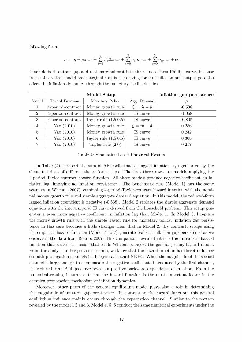
Model Setup in�ation gap persistenceModel Hazard Function Monetary Police Agg. Demand �

1 4-period-contract Money growth rule y = m� p -0.5382 4-period-contract Money growth rule IS curve -1.0683 4-period-contract Taylor rule (1.5,0.5) IS curve -0.8054 Yao (2010) Money growth rule y = m� p 0.2865 Yao (2010) Money growth rule IS curve 0.2426 Yao (2010) Taylor rule (1.5,0.5) IS curve 0.3087 Yao (2010) Taylor rule (2,0) IS curve 0.217

Table 4: Simulation based Empirical Results

In Table (4), I report the sum of AR coe¢ cients of lagged in�ations (�) generated by thesimulated data of di¤erent theoretical setups. The �rst three rows are models applying the4-period-Taylor-contract hazard function. All these models produce negative coe¢ cient on in-�ation lag, implying no in�ation persistence. The benchmark case (Model 1) has the samesetup as in Whelan (2007), combining 4-period-Taylor-contract hazard function with the nomi-nal money growth rule and simple aggregate demand equation. In this model, the reduced-formlagged in�ation coe¢ cient is negative (-0.538). Model 2 replaces the simple aggregate demandequation with the intertemporal IS curve derived from the household problem. This setup gen-erates a even more negative coe¢ cient on in�ation lag than Model 1. In Model 3, I replacethe money growth rule with the simple Taylor rule for monetary policy. in�ation gap persis-tence in this case becomes a little stronger than that in Model 2. By contrast, setups usingthe empirical hazard function (Model 4 to 7) generate realistic in�ation gap persistence as weobserve in the data from 1986 to 2007. This comparison reveals that it is the unrealistic hazardfunction that drives the result that leads Whelan to reject the general-pricing-hazard model.From the analysis in the previous section, we know that the hazard function has direct in�uenceon both propagation channels in the general-hazard NKPC. When the magnitude of the secondchannel is large enough to compensate the negative coe¢ cients introduced by the �rst channel,the reduced-form Phillips curve reveals a positive backward-dependence of in�ation. From thenumerical results, it turns out that the hazard function is the most important factor in thecomplex propagation mechanism of in�ation dynamics.

Moreover, other parts of the general equilibrium model plays also a role in determiningthe magnitude of in�ation gap persistence. In contrast to the hazard function, this generalequilibrium in�uence mainly occurs through the expectation channel. Similar to the patternrevealed by the model 1 2 and 3, Model 4, 5, 6 conduct the same numerical experiments under the

17

empirically based hazard function. In the model 4, the reduced-form lagged in�ation coe¢ cient ispositive (0.286). Model 5 replaces the simple demand equation with the IS curve and generates aslightly less in�ation gap persistence than Model 4. The reason why in�ation becomes even lesspersistent is that, with the intertemporal optimizing IS curve, demand shocks are not propagatedcompletely to output gap and in�ation dynamics, but they are partially dampened by the rise ofreal interest rate. So that expectational channel becomes less powerful than the previous case. InModel 6, I replace the money growth rule with the simple Taylor rule. in�ation gap persistencein this case becomes a little stronger than that in Model 4. The Taylor rule changes in�ationgap persistence, because it introduces an extra channel, through which in�ation and real forcesfeedback to the economy, so that the expectation channel is strengthened. In addition, in Model7, I apply another Taylor rule with a stronger in�ation response parameter and a zero responseparameter to output gap. Shutting down the feedback of output gap to the interest rate rulemakes the Taylor rule less powerful, so that it performs similar to the money growth rule.

In conclusion, both monetary policy rule and demand side of economy are important inpropagating in�ation dynamics, but the fundamentally important factor in this mechanism is thehazard function. Using the empirically based hazard function along with the Taylor rule and IScurve (Model 6), the general-pricing-hazard model preforms best in replicating the stylized factof in�ation gap persistence found in the U.S. CPI data from 1986 to 2007. It is not a surprisingresult, because most macroeconomists agree that monetary policy is well approximated by thesimple Taylor rule with coe¢ cients conforming to the Taylor principle during this period of time.In addition, this time span is also characterized by low and stable trend in�ation. This characterof data validates the use of the general-pricing-hazard model.

5 Conclusion

In this paper, I investigate whether the general-hazard NKPC is capable of accounting for thein�ation gap persistence. In the empirical part, I �nd that, after detrending in�ation by theCogley-Sbordone method, in�ation gap persistence is still signi�cant and large in the U.S. CPIdata. In the theoretical part, I redo the general equilibrium analysis by Whelan (2007), and checkrobustness of the result to di¤erent setups of the model. I �nd that the general-pricing-hazardmodel with empirically based price reset hazard function can account quite will for in�ationgap persistence found in the data of post Volcker�s disin�ation periods. The key mechanism atwork in this model is the expectational channel in the generalized NKPC, which depends on thesetup of the whole model, therefore in�ation gap persistence is also not independent of monetarypolicy. This result directly implies that the hybrid sticky price model should be subject to theLucas critique, and thereby can not be used in the monetary policy analysis.

However, one should also be aware of the limitation of the model. It can not account for time-varing trend in�ation, which a¤ects also the coe¢ cients in the NKPC (Cogley and Sbordone,2008). As a result, the general-pricing-hazard model is only suitable to model a economy witha stable monetary policy regime.

18

References

Altissimo, F., L. Bilke, A. Levin, T. Mathä, and B. Mojon (2006), Sectoral and aggregatein�ation dynamics in the euro area, Journal of the European Economic Association, 4(2-3),585�593.

Alvarez, L. J. (2007), What do micro price data tell us on the validity of the new keynesianphillips curve?, Kiel working papers, Kiel Institute for the World Economy.

Alvarez, L. J., E. Dhyne, M. Hoeberichts, C. Kwapil, H. L. Bihan, P. Lünnemann,F. Martins, R. Sabbatini, H. Stahl, P. Vermeulen, and J. Vilmunen (2006), Stickyprices in the euro area: A summary of new micro-evidence, Journal of the European EconomicAssociation, 4(2-3), 575�584.

Andrews, D. W. and H.-Y. Chen (1992), Approximately median-unbiased estimation of au-toregressive models with applications to u.s. macroeconomic and �nancial time series, CowlesFoundation Discussion Papers 1026, Cowles Foundation, Yale University.

Ascari, G. (2004), Staggered prices and trend in�ation: Some nuisances, Review of EconomicDynamics, 7(3), 642�667.

Bils, M. and P. J. Klenow (2004), Some evidence on the importance of sticky prices, Journalof Political Economy , 112(5), 947�985.

Calvo, G. A. (1983), Staggered prices in a utility-maximizing framework, Journal of MonetaryEconomics, 12(3), 383�98.

Carvalho, C. (2006), Heterogeneity in price stickiness and the real e¤ects of monetary shocks,The B.E. Journal of Macroeconomics, 0(1).

Cecchetti, S. G. (1986), The frequency of price adjustment : A study of the newsstand pricesof magazines, Journal of Econometrics, 31(3), 255�274.

Christiano, L. J., M. Eichenbaum, and C. L. Evans (2005), Nominal rigidities and thedynamic e¤ects of a shock to monetary policy, Journal of Political Economy , 113(1), 1�45.

Coenen, G., A. T. Levin, and K. Christo¤el (2007), Identifying the in�uences of nominaland real rigidities in aggregate price-setting behavior, Journal of Monetary Economics, 54(8),2439�2466.

Cogley, T., G. E. Primiceri, and T. J. Sargent (2008), In�ation-gap persistence in the u.s,NBER Working Papers 13749, National Bureau of Economic Research, Inc.

Cogley, T. and A. M. Sbordone (2008), Trend in�ation, indexation, and in�ation persistencein the new keynesian phillips curve, American Economic Review , 98(5), 2101�26.

Dixit, A. K. and J. E. Stiglitz (1977), Monopolistic competition and optimum productdiversity, American Economic Review , 67(3), 297�308.

19

Fuhrer, J. and G. Moore (1995), In�ation persistence, The Quarterly Journal of Economics,110(1), 127�59.

Fuhrer, J. C. (2006), Intrinsic and inherited in�ation persistence, International Journal ofCentral Banking , 2(3).

Gali, J. and M. Gertler (1999), In�ation dynamics: A structural econometric analysis, Jour-nal of Monetary Economics, 44(2), 195�222.

Kiley, M. T. (2002), Partial adjustment and staggered price setting, Journal of Money, Creditand Banking , 34(2), 283�98.

Levin, A. and J. Piger (2003), Is in�ation persistence intrinsic in industrial economies?,Computing in Economics and Finance 2003 298, Society for Computational Economics.

Lucas, R. J. (1972), Expectations and the neutrality of money, Journal of Economic Theory ,4(2), 103�124.

Nakamura, E. and J. Steinsson (2008), Five facts about prices: A reevaluation of menu costmodels, The Quarterly Journal of Economics, 123(4), 1415�1464.

Sheedy, K. D. (2007), Intrinsic in�ation persistence, CEP Discussion Papers dp0837, Centrefor Economic Performance, LSE.

Taylor, J. B. (1993), Discretion versus policy rules in practice, Carnegie-Rochester ConferenceSeries on Public Policy , 39, 195�214.

Whelan, K. (2007), Staggered price contracts and in�ation persistence: Some general results,International Economic Review , 48(1), 111�145.

Wolman, A. L. (1999), Sticky prices, marginal cost, and the behavior of in�ation, EconomicQuarterly , (Fall), 29�48.

Yao, F. (2010), Aggregate hazard function in price-setting: A bayesian analysis using macrodata, SFB 649 Discussion Papers 2010-020, Humboldt University, Berlin, Germany.

20

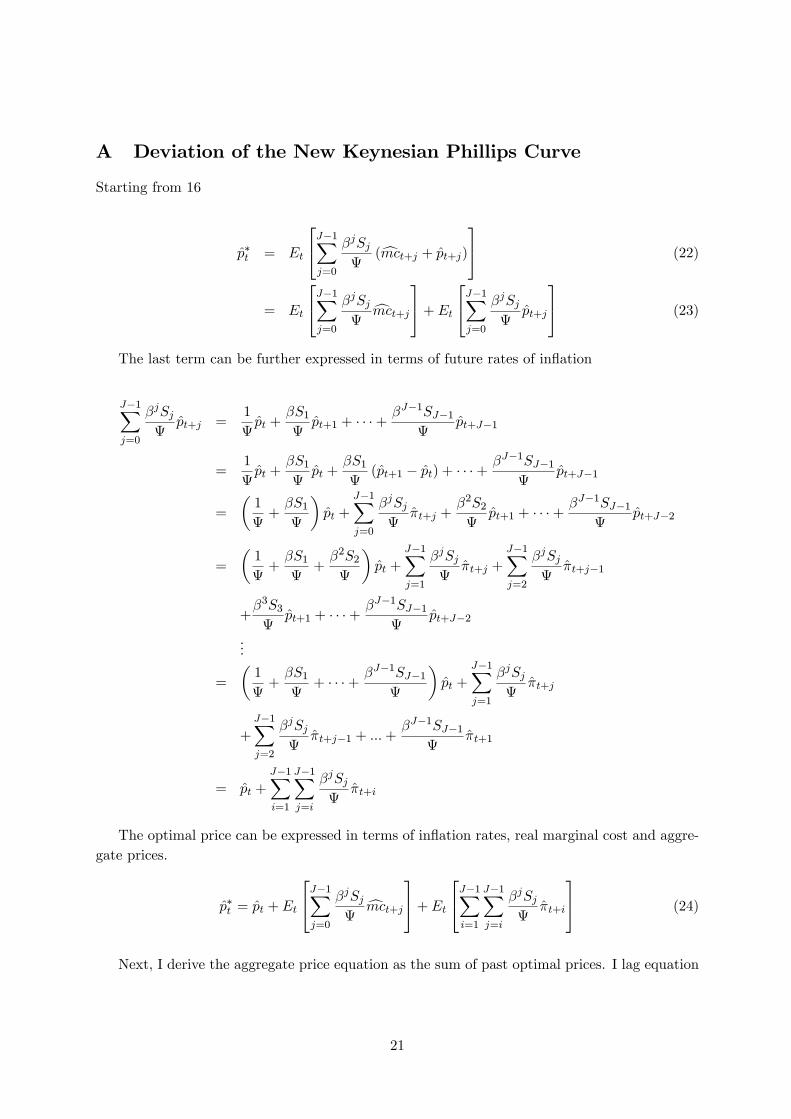
A Deviation of the New Keynesian Phillips Curve

Starting from 16

p�t = Et

24J�1Xj=0

�jSj

(cmct+j + pt+j)35 (22)

= Et

24J�1Xj=0

�jSj

cmct+j35+ Et

24J�1Xj=0

�jSj

pt+j

35 (23)

The last term can be further expressed in terms of future rates of in�ation

J�1Xj=0

�jSj

pt+j =1

pt +

�S1pt+1 + � � �+

�J�1SJ�1

pt+J�1

=1

pt +

�S1pt +

�S1(pt+1 � pt) + � � �+

�J�1SJ�1

pt+J�1

=

�1

+�S1

�pt +

J�1Xj=0

�jSj

�t+j +�2S2

pt+1 + � � �+�J�1SJ�1

pt+J�2

=

�1

+�S1

+�2S2

�pt +

J�1Xj=1

�jSj

�t+j +J�1Xj=2

�jSj

�t+j�1

+�3S3

pt+1 + � � �+�J�1SJ�1

pt+J�2

...

=

�1

+�S1

+ � � �+ �J�1SJ�1

�pt +

J�1Xj=1

�jSj

�t+j

+

J�1Xj=2

�jSj

�t+j�1 + :::+�J�1SJ�1

�t+1

= pt +J�1Xi=1

J�1Xj=i

�jSj

�t+i

The optimal price can be expressed in terms of in�ation rates, real marginal cost and aggre-gate prices.

p�t = pt + Et

24J�1Xj=0

�jSj

cmct+j35+ Et

24J�1Xi=1

J�1Xj=i

�jSj

�t+i

35 (24)

Next, I derive the aggregate price equation as the sum of past optimal prices. I lag equation

21

24 and substitute it for each p�t�j into equation 17

pt = �(0) p�t + �(1) p�t�1 + � � �+ �(J � 1)p�t�J+1

= �(0)

24pt + Et0@J�1Xj=0

�jSj

cmct+j1A+ Et

0@J�1Xi=1

J�1Xj=i

�jSj

�t+i

1A35+ �(1)

24pt�1 + Et�10@J�1Xj=0

�jSj

cmct+j�11A+ Et�1

0@J�1Xi=1

J�1Xj=i

�jSj

�t+i�1

1A35...

+ �(J � 1)

24pt�J+1 + Et�J+10@J�1Xj=0

�jSj

cmct+j�J+11A+ Et�J+1

0@J�1Xi=1

J�1Xj=i

�jSj

�t+i�J+1

1A35

pt =

J�1Xk=0

�(k)

2666664pt�k + Et�k0@J�1Xj=0

�jSj

cmct+j�k + J�1Xi=1

J�1Xj=i

�jSj

�t+i�k

1A| {z }

Ft�k

3777775 (25)

Where Ft summarizes all current and lagged expectations formed at period t.Finally, we derive the New Keynesian Phillips curve from equation 25.

pt =

J�1Xk=0

�(k) pt�k +J�1Xk=0

�(k)Ft�k| {z }Qt

�t =

J�1Xk=0

�(k) pt�k � pt�1 +Qt

= �(0) (pt � pt�1) + �(0)pt�1 + �(1)pt�1 + � � �+ �(J � 1)pt�J+1 � pt�1 +Qt= �(0) (pt � pt�1) + (�(0) + �(1)) pt�1 + �(2)pt�2 + � � �+ �(J � 1)pt�J+1 � pt�1 +Qt= �(0)|{z}

W (0)

�t + (�(0) + �(1))| {z } �t�1+W (1)

(�(0) + �(1) + �(2)) pt�2 � � �+ �(J � 1)pt�J+1 � pt�1 +Qt

...

= W (0) �t +W (1)�t�1 + � � �+W (J � 2)�t�J+2 +W (J � 1)| {z }=1

pt�J+1 � pt�1 +Qt

= W (0) �t + � � �+W (J � 2)�t�J+2 + pt�J+1 � pt�J+2| {z }��t�J+2

+ pt�J+2 � � � �+ pt�2 � pt�1| {z }��t�1

+Qt

(1�W (0))�t = �(1�W (2))�t�1 � � � � � (1�W (J � 1))�t�J+2 +Qt

�t = �J�1Xk=2

1�W (k)1� �(0) �t�k+1 +

J�1Xk=0

�(k)

1� �(0)Ft�k

The general-hazard New Keynesian Phillips curve is:

22

�t =

J�1Xk=0

�(k)

1� �(0)Et�k

0@J�1Xj=0

�jSj

cmct+j�k + J�1Xi=1

J�1Xj=i

�jSj

�t+i�k

1A

�J�1Xk=2

�(k)�t�k+1; where �(k) =

J�1Pj=k

Sj

J�1Pj=1Sj

; =

J�1Xj=0

�jSj (26)

23

B Proof

In the Calvo pricing case, all hazards are equal to a constant between zero and one. Denote theconstant hazard as h = 1� �, and substitute it into the NKPC (18):

�t +1Xk=1

�k�t�k = (1� �)1Xk=0

�kEt�k

(1� ��)

1Xi=0

�i�imct+i�k +1Xi=0

�i�i�t+i�k

!

�t + ��t�1 + �2�t�2 + � � � = Et

(1� �)(1� ��)

1Xi=0

�i�imct+i + (1� �)1Xi=0

�i�i�t+i

!

+ �Et�1

(1� �)(1� ��)

1Xi=0

�i�imct+i�1 + (1� �)1Xi=0

�i�i�t+i�1

!

+ �2Et�2

(1� �)(1� ��)

1Xi=0

�i�imct+i�2 + (1� �)1Xi=0

�i�i�t+i�2

!...: (27)

Iterate this equation one period forward, I obtain

�t+1 + ��t + �2�t�1 + �

3�t�2 � � � = Et+1

(1� �)(1� ��)

1Xi=0

�i�imct+i+1 + (1� �)1Xi=0

�i�i�t+i+1

!

+ �Et

(1� �)(1� ��)

1Xi=0

�i�imct+i + (1� �)1Xi=0

�i�i�t+i

!

+ �2Et�1

(1� �)(1� ��)

1Xi=0

�i�imct+i�1 + (1� �)1Xi=0

�i�i�t+i�1

!...:

Use equation (27) to substitute terms in the left hand side of the equation (�t; �t�1; �t�2 � � � ), Iget

24

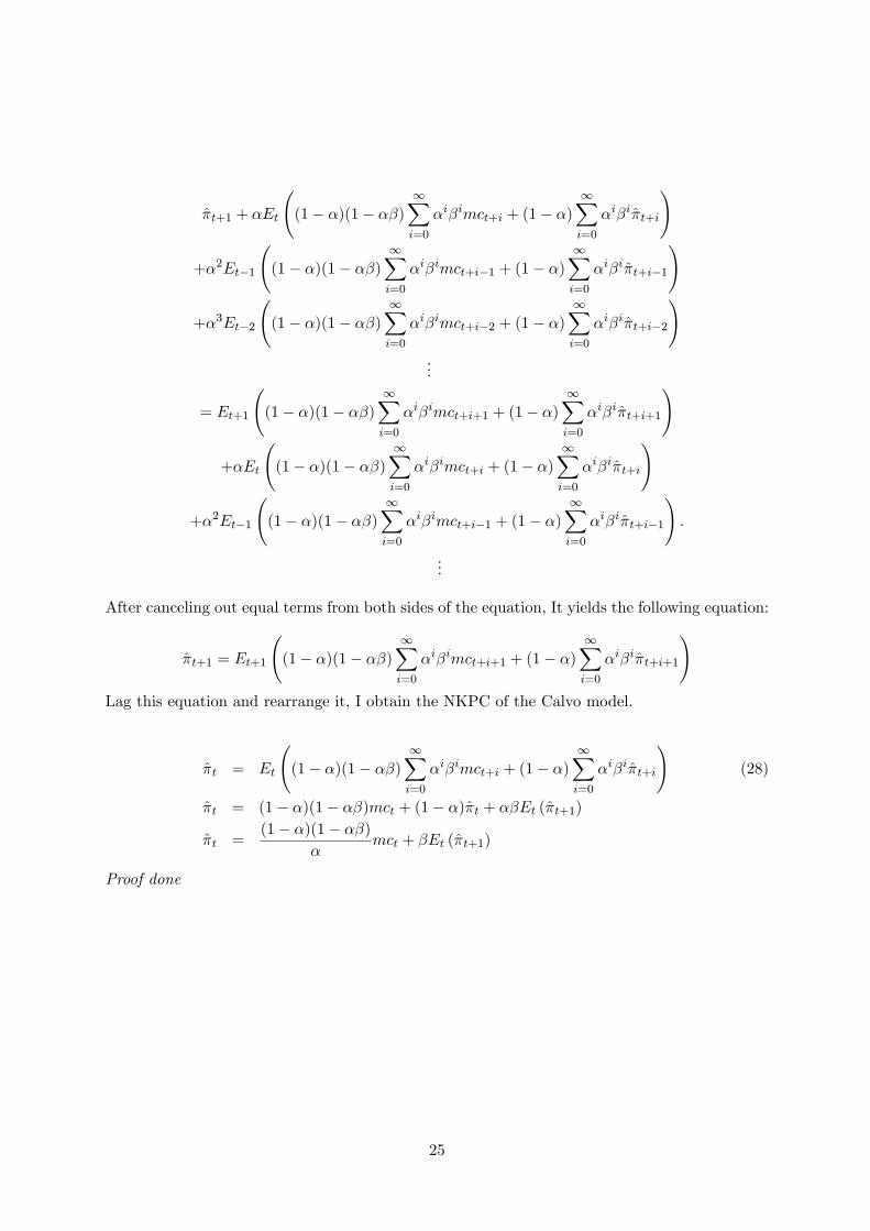
�t+1 + �Et

(1� �)(1� ��)

1Xi=0

�i�imct+i + (1� �)1Xi=0

�i�i�t+i

!

+�2Et�1

(1� �)(1� ��)

1Xi=0

�i�imct+i�1 + (1� �)1Xi=0

�i�i�t+i�1

!

+�3Et�2

(1� �)(1� ��)

1Xi=0

�i�imct+i�2 + (1� �)1Xi=0

�i�i�t+i�2

!...

= Et+1

(1� �)(1� ��)

1Xi=0

�i�imct+i+1 + (1� �)1Xi=0

�i�i�t+i+1

!

+�Et

(1� �)(1� ��)

1Xi=0

�i�imct+i + (1� �)1Xi=0

�i�i�t+i

!

+�2Et�1

(1� �)(1� ��)

1Xi=0

�i�imct+i�1 + (1� �)1Xi=0

�i�i�t+i�1

!:

...

After canceling out equal terms from both sides of the equation, It yields the following equation:

�t+1 = Et+1

(1� �)(1� ��)

1Xi=0

�i�imct+i+1 + (1� �)1Xi=0

�i�i�t+i+1

!Lag this equation and rearrange it, I obtain the NKPC of the Calvo model.

�t = Et

(1� �)(1� ��)

1Xi=0

�i�imct+i + (1� �)1Xi=0

�i�i�t+i

!(28)

�t = (1� �)(1� ��)mct + (1� �)�t + ��Et (�t+1)

�t =(1� �)(1� ��)

�mct + �Et (�t+1)

Proof done

25

001 "Volatility Investing with Variance Swaps" by Wolfgang Karl Härdle and Elena Silyakova, January 2010.

002 "Partial Linear Quantile Regression and Bootstrap Confidence Bands" by Wolfgang Karl Härdle, Ya’acov Ritov and Song Song, January 2010.

003 "Uniform confidence bands for pricing kernels" by Wolfgang Karl Härdle, Yarema Okhrin and Weining Wang, January 2010.

004 "Bayesian Inference in a Stochastic Volatility Nelson-Siegel Model" by Nikolaus Hautsch and Fuyu Yang, January 2010.

005 "The Impact of Macroeconomic News on Quote Adjustments, Noise, and Informational Volatility" by Nikolaus Hautsch, Dieter Hess and David Veredas, January 2010.

006 "Bayesian Estimation and Model Selection in the Generalised Stochastic Unit Root Model" by Fuyu Yang and Roberto Leon-Gonzalez, January 2010.

007 "Two-sided Certification: The market for Rating Agencies" by Erik R. Fasten and Dirk Hofmann, January 2010.

008 "Characterising Equilibrium Selection in Global Games with Strategic Complementarities" by Christian Basteck, Tijmen R. Daniels and Frank Heinemann, January 2010.

009 "Predicting extreme VaR: Nonparametric quantile regression with refinements from extreme value theory" by Julia Schaumburg, February 2010.

010 "On Securitization, Market Completion and Equilibrium Risk Transfer" by Ulrich Horst, Traian A. Pirvu and Gonçalo Dos Reis, February 2010.

011 "Illiquidity and Derivative Valuation" by Ulrich Horst and Felix Naujokat, February 2010.

012 "Dynamic Systems of Social Interactions" by Ulrich Horst, February 2010.

013 "The dynamics of hourly electricity prices" by Wolfgang Karl Härdle and Stefan Trück, February 2010.

014 "Crisis? What Crisis? Currency vs. Banking in the Financial Crisis of 1931" by Albrecht Ritschl and Samad Sarferaz, February 2010.

015 "Estimation of the characteristics of a Lévy process observed at arbitrary frequency" by Johanna Kappusl and Markus Reiß, February 2010.

016 "Honey, I’ll Be Working Late Tonight. The Effect of Individual Work Routines on Leisure Time Synchronization of Couples" by Juliane Scheffel, February 2010.

017 "The Impact of ICT Investments on the Relative Demand for High-Medium-, and Low-Skilled Workers: Industry versus Country Analysis" by Dorothee Schneider, February 2010.

018 "Time varying Hierarchical Archimedean Copulae" by Wolfgang Karl Härdle, Ostap Okhrin and Yarema Okhrin, February 2010.

019 "Monetary Transmission Right from the Start: The (Dis)Connection Between the Money Market and the ECB’s Main Refinancing Rates" by Puriya Abbassi and Dieter Nautz, March 2010.

020 "Aggregate Hazard Function in Price-Setting: A Bayesian Analysis Using Macro Data" by Fang Yao, March 2010.

021 "Nonparametric Estimation of Risk-Neutral Densities" by Maria Grith, Wolfgang Karl Härdle and Melanie Schienle, March 2010.

SFB 649 Discussion Paper Series 2010

For a complete list of Discussion Papers published by the SFB 649, please visit http://sfb649.wiwi.hu-berlin.de.

SFB 649 Discussion Paper Series 2010

For a complete list of Discussion Papers published by the SFB 649, please visit http://sfb649.wiwi.hu-berlin.de.

022 "Fitting high-dimensional Copulae to Data" by Ostap Okhrin, April 2010. 023 "The (In)stability of Money Demand in the Euro Area: Lessons from a

Cross-Country Analysis" by Dieter Nautz and Ulrike Rondorf, April 2010. 024 "The optimal industry structure in a vertically related market" by

Raffaele Fiocco, April 2010. 025 "Herding of Institutional Traders" by Stephanie Kremer, April 2010. 026 "Non-Gaussian Component Analysis: New Ideas, New Proofs, New

Applications" by Vladimir Panov, May 2010. 027 "Liquidity and Capital Requirements and the Probability of Bank Failure"

by Philipp Johann König, May 2010. 028 "Social Relationships and Trust" by Christine Binzel and Dietmar Fehr,

May 2010. 029 "Adaptive Interest Rate Modelling" by Mengmeng Guo and Wolfgang Karl

Härdle, May 2010. 030 "Can the New Keynesian Phillips Curve Explain Inflation Gap

Persistence?" by Fang Yao, June 2010.