Esri Trend Analysis: 2010- · PDF fileEsri Trend Analysis: 2010–2015 Esri, ... Data sources are ... homes.5 Since April was the last month to take advantage of the tax credits for

An Esri

® White Paper • June 2010

Esri Trend Analysis: 2010–2015

Esri, 380 New York St., Redlands, CA 92373-8100 USA TEL 909-793-2853 • FAX 909-793-5953 • E-MAIL [email protected] • WEB www.esri.com

Copyright © 2010 Esri All rights reserved. Printed in the United States of America. The information contained in this document is the exclusive property of Esri. This work is protected under United States copyright law and other international copyright treaties and conventions. No part of this work may be reproduced or transmitted in any form or by any means, electronic or mechanical, including photocopying and recording, or by any information storage or retrieval system, except as expressly permitted in writing by Esri. All requests should be sent to Attention: Contracts and Legal Services Manager, Esri, 380 New York Street, Redlands, CA 92373-8100 USA. The information contained in this document is subject to change without notice. Esri, the Esri globe logo, Tapestry, www.esri.com, and @esri.com are trademarks, registered trademarks, or service marks of Esri in the United States, the European Community, or certain other jurisdictions. Other companies and products mentioned herein may be trademarks or registered trademarks of their respective trademark owners.

J-9926

Esri White Paper i


An Esri White Paper Contents Page Current Trends ...................................................................................... 1 Past Trends: Decade in Review ............................................................ 5 The Economic Outlook ......................................................................... 8 Geography Changes in 2010................................................................. 11 Esri's Data Development Team............................................................. 12

J-9926

Esri White Paper


Current Trends Whether the Great Recession has ended remains debatable in the second quarter of 2010, though many economists believe that the recession, begun in December 2007, probably ended sometime in the third or fourth quarter of 2009. Recovery also remains debatable. Fears over a double-dip recession persist. Data sources are contradictory: ■ Gross domestic product (GDP) rose by 2.7 percent in the first quarter of 2010, a real

improvement over the first quarter of 2009, which saw a decline of 6.4 percent, but less than expected and less than the fourth quarter of 2009, in which the GDP rose by 5.6 percent.1

■ Stock markets remain volatile. Within two weeks in June, the Dow Jones industrial

average dropped to a seven-month low of 9,816, then climbed to 10,450—significant, but hardly comparable to the flash crash of May 6, when the Dow lost almost 1,000 points in less than 10 minutes.

■ Unemployment claims dropped by a quarter of a million at the end of May 2010.

That month also posted the largest increase in jobs since March 2000, a gain of 431,000. However, almost all the new jobs (411,000) were temporary census jobs. Private employers added only 41,000 jobs, down from 218,000 in April. Other government jobs (state and local) declined by 21,000.2 Weekly jobless claims increased again in mid-June.3

■ Consumer confidence increased from March through May, rising to 62.7, but retail

sales fell by 1.2 percent in May—the first time in eight months and contrary to expectations.4

■ Sales of new and existing homes exceeded expectations in March and April, posting

year-over-year April increases of 48 percent for new and 23 percent for existing homes.5 Since April was the last month to take advantage of the tax credits for home buyers, the outlook for the rest of the year is more guarded. Sales in May dropped by 2.2 percent for existing homes and 33 percent for new homes (a record drop). Housing inventories remain high.

1 http://money.cnn.com/2010/04/30/news/economy/gdp/index.htm?postversion=2010043010;

http://money.cnn.com/2010/05/27/news/economy/gdp/index.htm. 2 http://money.cnn.com/2010/06/04/news/economy/jobs_may/index.htm. 3 http://www.dol.gov/opa/media/press/eta/ui/eta20100816.htm. 4 http://money.cnn.com/2010/05/25/news/economy/consumer_confidence/index.htm.

Note: Consumer confidence fell to 52.9 in June—http://money.cnn.com/2010/06/29/news/economy/ consumer_confidence/index.htm?source=cnn_bin&hpt=Sbin.

5 http://money.cnn.com/2010/05/26/news/economy/new_home_sales/index.htm.


J-9926

June 2010 2

■ Foreclosures declined by 3 percent in May, but the activity level remained at more than 300,000 filings for the fifteenth straight month. Bank repossessions increased.6

What, exactly, is happening? The economy appears to be recovering, but growth is tepid and inconsistent across the country: ■ Population growth has resumed or increased in about one-third of counties, but more

than half of the counties are still experiencing loss of population. ■ Curiously, the housing inventory increased in more than 85 percent of counties from

2009 to 2010. Vacancy rates also increased in more than 85 percent of counties. ■ The free fall in median home value that hit two-thirds of counties from 2008 to 2009

has stabilized and reversed in almost one-fourth of counties in 2010. Recent gains in these counties are moderate, with an average of 2.4 percent.

■ Ninety-five percent of counties experienced a loss of jobs from 2008 to 2009. One

year later, more than half of the counties are currently showing some gain in employment, with a collective increase of 1.7 million, or 2.8 percent. The other half of the counties experienced a collective loss of 2.3 million jobs, for a net loss of almost 600,000 jobs.

■ Unemployment rates increased in 97 percent of counties from 2008 to 2009. Almost

40 percent of counties now have declining rates of unemployment, officially. (These rates do not include workers that have dropped off the unemployment rolls or left the labor force.)

■ The effects of a recession on annual household income are not immediate.7 From

2008 to 2009, 37 percent of counties experienced a decline in median household income. The decreases generally ranged from $1 to $250. Last year, more than 98 percent of counties lost income. The decrease in median household income ranged from $1 to $1,700.

Some improvement is evident, but so is the continued loss, especially in jobs and income; for every step forward, there are two steps backward. At the county level, the changes appear to be variable. At the metropolitan level, a clearer pattern of change emerges. Table 1 shows the initial harbingers of the recession—population change and home value—and two key consequences, employment and household income.

Table 1 Change 2008–2010 by Metropolitan Status

Counties by Metropolitan Status Annual Change (%)

Metropolitan Micropolitan Nonmetropolitan Population 2009–2010 0.6 0.1 -0.6 2008–2009 0.2 -0.1 -0.6

6 http://www.realtytrac.com/contentmanagement/pressrelease.aspx?channelid=9&itemid=9427. 7 Household income remains consistent with Census 2000 definitions: income in the previous year. The 2010

income updates actually represent income in 2009.


J-9926

Esri White Paper 3

Counties by Metropolitan Status Annual Change (%) Metropolitan Micropolitan Nonmetropolitan

Median Home Value 2009–2010 -2.9 -1.7 -2.2 2008–2009 -12.8 -2.0 -1.1

Employment 2009–2010 -0.6 0.4 0.6 2008–2009 -3.9 -4.0 -4.3

Median Household Income

2009–2010 -0.7 -0.4 -0.5 2008–2009 -0.4 0.4 0.7

Number of Counties 1,100 688 1,353 Deceleration in home value appreciation and population growth presaged the Great Recession as early as 2006–2007. These changes initially affected the hottest markets—primarily metropolitan markets in the South and West. Over the next three years, the decline snowballed from smaller rates of growth to loss and spread into micropolitan and nonmetropolitan counties. The depreciation in home value has slowed significantly among metropolitan counties. The smaller micropolitan and nonmetropolitan counties were less affected by the swings in the housing market: less appreciation during the housing bubble and less deflation on the downside. Home price fluctuations in less populous markets have been significantly milder than in metropolitan areas, but in the last year, prices fell at twice the rate of those in 2008–2009. Micropolitan areas maintained an annual loss of almost 2 percent over the last two years, while metropolitan areas improved from -12.8 percent between 2008 and 2009 to only -3 percent. Home value is gradually stabilizing, and population growth is improving, with a slight increase among metropolitan counties and a shift from minus to plus among micropolitan counties. Nonmetropolitan counties continue to lose population. The economic crisis that ensued from the collapse of the housing market is still affecting all counties. In 2009, rising unemployment augmented the rise in foreclosures, depressed population growth further, and diffused that trend to 80 percent of counties and 82 percent of metropolitan markets. In 2010, employment is still decreasing among metropolitan counties, but there have been slight gains in employment among the micropolitan and nonmetropolitan markets. The shift is moderate and insufficient to stem rising unemployment rates. The consequence of unemployment—income loss—is also evident now. Median household income is declining among all counties; however, it is more pronounced among metropolitan counties. Only metropolitan areas experienced an income decline in the first full recession year. In 2009, median income fell in metropolitan, micropolitan, and nonmetropolitan areas. The rate of decline in metropolitan areas still exceeds micropolitan and nonmetropolitan areas by 0.3 and 0.2 percentage points, respectively. This is likely a result of the concentration of job losses and business failures in metropolitan areas where financial, retail, service, and construction sectors, all heavily impacted by the downturn, are clustered. At the national level, median household income fell by half of a percentage point to $54,442.


J-9926

June 2010 4

Figure 1 2010 Median Household Income in the United States

By region, the distinctions are less pronounced, as shown in table 2. Population growth has resumed in each of the regions; however, the current change in home value remains negative across the regions—improving, but still negative.8 Employment is now showing improvement in the Northeast, South, and West. The Midwest is still experiencing significant job losses. Much of this year's job loss came from this area, which shed over 564,000 positions, led by Illinois, Ohio, Missouri, and Michigan. In the South, states are recovering much better relative to 2009; some states are starting to post gains. The net increase in job creation is nearly 60,000 workers, primarily from Texas and the Carolinas. Florida and Georgia are still experiencing difficulties jump-starting their economies. Household income is increasing again in the Northeast, but the other regions are now feeling the recessionary effects.

8 Regions are a geographic classification; metropolitan areas represent a demographic grouping. The

distinctions in demographic measures are likely to differ. The Northeast and West have the highest concentrations of population in metropolitan areas, almost 90 percent. The Midwest and South have less than 80 percent of their populations in metropolitan areas.


J-9926

Esri White Paper 5

Table 2 Change 2008–2010 by Region

Region Annual Change (%)

Northeast Midwest South West Population 2009–2010 0.1 0.1 0.8 0.6 2008–2009 -0.4 -0.4 0.4 0.6

Median Home Value 2009–2010 -2.6 -1.3 -2.6 -3.8 2008–2009 -6.0 -6.6 -10.8 -19.4

Employment 2009–2010 -0.1 -1.8 0.1 -0.2 2008–2009 -3.8 -3.7 -3.9 -4.3

Median Household Income

2009–2010 0.7 -0.9 -0.6 -1.1 2008–2009 -0.1 0.0 0.1 0.0

Past Trends: Decade

in Review The past decade includes the extremes of a growth cycle: phenomenal growth and a spectacular crash. What is the balance—net gain, net loss—or did we break even? From 2000 to 2010, changes include some interesting increases:

■ Total population: An average annual increase of less than 1 percent ■ Housing units: +14 percent ■ Vacant housing units: +52 percent ■ Median home value: +41 percent ■ Civilian employment: +5 percent ■ Unemployment: +107 percent ■ Median household income: +29 percent


J-9926

June 2010 6

Figure 2 2000–2010 Population Growth in the United States

It's not difficult to see the problems inherent in a 52 percent increase in vacant housing or a 107 percent increase in the number of unemployed workers compared to a gain of less than 5 percent in jobs. However, it's difficult to assess an increase of more than 40 percent in home value or almost 30 percent in household income without a comparison. The following chart compares change in select indicators in the current decade, 2000–2010, to the previous decade, 1990–2000. Both decades began with comparatively mild recessions. The singular differences between the two periods are the housing bubble and the Great Recession.


J-9926

Esri White Paper 7

Chart 1 Percent Change in Select Indicators by Decade

Although the net gain from 2000 to 2010 is less than the growth in the 1990s, there is variation. Home price fluctuations have hit historic extremes, both positive and negative, during the last decade. The net gain is 41 percent since 2000, comparable to the gain between 1990 and 2000. Median home value for 2010 stands at $157,910, reflecting an average annual change of 3.4 percent since 2000. Neither the growth induced by the housing bubble nor the recession has affected all areas equally. Massive swings in home prices occurred among the fastest-growing states in both periods, measured by rate (Arizona, Nevada) or absolute numbers (California, Florida). These states also had skyrocketing foreclosure filings after 2007.9 Prior to 2007, the states experienced year-on-year appreciation reaching 20 to 30 percent, before the crash. Fueled by early gains this decade, California and Florida maintained reasonable 10-year appreciation of 5 and 3 percent annually, respectively. Michigan is the only state that showed virtually no appreciation in the last 10 years—incomparable to the 90 percent gain during the 1990s. Michigan was impacted not only by the housing crisis but also by the auto industry's troubles. The Detroit Metropolitan Area alone experienced a home price drop of almost 15 percent. In fact, the city of Detroit recently announced plans to downsize, a reversal program in which acres of abandoned properties will be demolished and the land restored to fields and farmland.10 Employment provides a less favorable comparison between 2000–2010 and 1990–2000. The net gain in jobs for the 2000–2010 decade was just 6.3 million. The increase in unemployment was 8.5 million workers, or an increase in the unemployment rate of 5 percentage points. Contrast this performance with the 1990s, when the private economy produced more than twice as many jobs (14 million) and the rate of unemployment improved by half of a percentage point from 6.3 percent to 5.8 percent. The downturn in

9 The notable exception to this association is Texas, which has been not only one of the fastest-growing states

by rate or number but also one of the states least affected by foreclosure filings. 10http://www.washingtontimes.com/news/2010/mar/09/detroit-looks-at-downsizing-to-save-city/.


J-9926

June 2010 8

employment is wholly the result of the recession. Through July 2007, employment had increased by almost 11.9 million jobs. A comparison of the last two decades suggests that the shape of the income distribution has already experienced more permanent change. During the 1990s, median household income grew at 3.4 percent a year; average household income grew even faster at 3.9 percent. Since averages are readily influenced by extremes in the distribution, the conclusion is that the rich were getting richer while the poor were getting poorer. However, Esri estimates for the last decade show a significant change. Median household income grew at only 2.5 percent a year, barely keeping up with inflation, while average household income trailed, at a rate of 2.1 percent a year.

The Economic Outlook

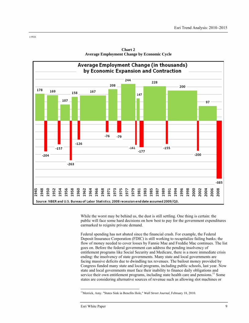
Uncertainty is the best outlook in the face of weak job growth, growing debt, and persistent concern over a double-dip recession. Declaring a recession is the purview of the National Bureau of Economic Research (NBER). It tracks quarterly GDP estimates, industrial production, manufacturing and trade sales, gross domestic income, personal income, and employment from the Current Employment Statistics payroll and Current Population Survey. All the indicators had turned around by the end of 2009, with the exception of employment. The monthly payroll survey and the household-based employment survey have just started to show signs of growth in 2010. There are other signs of improvement in the labor market. The number of temporary jobs has been rising since the third quarter of 2009. Typically, firms squeeze more output from their existing workforce when business is slow. As orders pick up and inventories reach lower levels, businesses can take a cautious, cost-effective approach by hiring temporary workers during the beginning stages of a recovery. Another positive sign is the four-week moving average of filers, both new and continuing, for unemployment insurance benefits: it has been on the decline since mid-2009. While the economic indicators, as well as the recent surge on Wall Street, suggest improving conditions, "Main Street" may disagree. Based on the jobs and homes lost during the recession, it is hard to dismiss such a perception. Before the 2008 downturn, the overall average monthly job loss of all post-World War II recessions was 160,000 positions. Assuming the 2008 recession ended in September 2009, the number of jobs lost in a typical month swells to a record high of 385,000. This makes the Great Recession the deepest contraction in monthly employment, as shown in chart 2.


J-9926

Esri White Paper 9

Chart 2 Average Employment Change by Economic Cycle

While the worst may be behind us, the dust is still settling. One thing is certain: the public will face some hard decisions on how best to pay for the government expenditures earmarked to reignite private demand. Federal spending has not abated since the financial crash. For example, the Federal Deposit Insurance Corporation (FDIC) is still working to recapitalize failing banks; the flow of money needed to cover losses by Fannie Mae and Freddie Mac continues. The list goes on. Before the federal government can address the pending insolvency of entitlement programs like Social Security and Medicare, there is a more immediate crisis ending: the insolvency of state governments. Many state and local governments are facing massive deficits due to dwindling tax revenues. The bailout money provided by Congress funded many state and local programs, including public schools, last year. Now state and local governments must face their inability to finance daily obligations and service their own entitlement programs, including state health care and pensions.11 Some states are considering alternative sources of revenue such as allowing slot machines or

11Merrick, Amy. "States Sink in Benefits Hole," Wall Street Journal, February 18, 2010.


J-9926

June 2010 10

taxing Internet retail sales transactions. In the end, the recession has exposed the shaky foundations of many state budgets. Current and future taxpayers face a growing mountain of debt due to the steps taken by the federal government to avert the financial crisis. The United States accumulated a record annual deficit of $1.4 trillion dollars in 2009. The White House's Office of Management and Budget (OMB) projects another record breaker in 2010. OMB estimates a debt level of $13.7 trillion, or 94 percent of GDP, which represents a 60-year high. OMB also projects continued growth in the public debt through 2015, when it tops out at nearly $20 trillion, or 103 percent of GDP. The Moody's rating agency has issued a warning: if reductions are not made, the U.S. government is at risk of losing its high credit rating.12 Such a downgrade would make additional borrowing more costly, compounding the debt problem. The federal government may hope to grow its way out of the problem but ultimately will face difficult choices on whether to reduce spending, increase taxes, or enact some combination of both. There is another, more sinister way to tackle debt: inflate it away. This concern is another reason investors are making moves to safeguard their portfolios from the potential erosion of purchasing power. The economy has slowly responded to efforts by the Federal Reserve, the U.S. Treasury, and Congress to counter the downturn. The real question is, How sustainable is the current nascent recovery? The housing market no longer appears to be in free fall, but foreclosures remain high. Sales in the past year have been fueled by the bargain appeal of bank repossessions and by tax incentives. Despite predictions that foreclosure activity would peak around the third quarter of 2009, various data sources suggest that the crisis is far from over. The Federal Housing Administration's (FHA) April 2010 Outlook confirms that 8.5 percent of its loans were seriously delinquent as of March 2010, an 80 percent increase year-on-year. RealtyTrac estimates that about 2.8 million homes were foreclosed in 2009 but projects an astounding 4.5 million foreclosure filings in 2010. President Barack Obama's foreclosure prevention initiative, Home Affordable Modification Program, introduced in early 2009, has steered over 100,000 loans toward lower interest rates or lengthened repayment terms. The program has helped a very small portion of homeowners at risk. With unemployment rates at historically high levels, even loan modifications have been insufficient to bail out the one in five homeowners estimated to owe more than their properties are worth. This program was made permanent in early 2010. Tax incentives for home buyers have been more effective in the past year. This popular program has helped the U.S. housing market begin the process of stabilization—showing a moderating decline in the last year. U.S home value is expected to decline another 2.7 percent between 2009 and 2010. This is an improvement over the 11.3 percent drop in the previous year. In the last year, 164 metropolitan markets showed gains in home value, compared to only 23 in the prior year. However, the end of the tax incentive program in April 2010 and the steady flow of foreclosure filings will continue downward pressure on home prices until the economy picks up and businesses begin hiring again.

12Jolly, David, and Catherine Rampell. "Moody's Says U.S. Debt Could Test Triple-A Rating," The New York

Times, March 15, 2010.


J-9926

Esri White Paper 11

Assuming a slow but steady rebound, Esri's five-year forecast of the U.S. labor market shows improvement. Between 2010 and 2015, the economy will create an additional 8.3 million new jobs, bringing the total to 144 million workers. The pool of unemployed workers is projected to shrink to roughly 14 million people and the unemployment rate to drop two percentage points to 8.8 percent. Challenges certainly loom ahead. During such a slow rebound, how will market participants respond to the possibility of higher tax rates in the future to finance the debt? The first test comes in January 2011, when former president George W. Bush's tax cuts on personal income, estates, dividends, and capital gains will expire. Will consumer spending and business investment recede, triggering another downturn? If so, the five-year outlook will look different from what we currently predict. Two-thirds of the national economy is driven by consumer spending. Consumer spending reflects the personal effects of the Great Recession. Just how much do these macro-level forces affect the individual household? The 2007 Survey of Consumer Finance estimates the impact: The average family has 61 percent of its assets in real estate and stocks. Since 66 percent of homes are owned, almost every American has experienced major losses in assets. According to the Consumer Confidence Index (CCI) from the Conference Board, consumer confidence hit a low rating of 25 in February 2009 and recovered to 62.7 in May 2010. A key economic indicator, the CCI measures consumers' optimism about the state of the economy, which translates into their patterns of saving and spending. Until the CCI reaches 90, a level of economic stability, households will watch their budgets closely. One thing is clear—this recession has changed us all.

Geography Changes in 2010

Change is inevitable with any geographic area—political or statistical. Identifying the changes in the areas for which data is tabulated and reported is critical to the analysis of trends. In the past year, there have been minor changes to metropolitan areas by OMB, boundary revisions for designated market areas (DMAs) by Nielsen Media Research, and the usual adjustment of ZIP Codes by the U.S. Postal Service. Metropolitan changes include the latest revisions to Core Based Statistical Areas (CBSAs), released in December 2009. Changes include two new micropolitan areas: Marble Falls, TX (CBSA Code 31920), and Weatherford, OK (CBSA Code 48220). There are also three name changes that include code revisions: North Port-Bradenton-Sarasota, FL, Metropolitan Statistical Area (CBSA Code 35840, formerly 14600); Crestview-Fort Walton Beach-Destin, FL, Metropolitan Statistical Area (CBSA Code 18880, formerly 23020); and Steubenville-Weirton, OH-WV, Metropolitan Statistical Area (CBSA Code 44600, formerly 48260), plus 10 other name changes. There are 942 Core Based Statistical Areas, 366 metropolitan areas, and 576 micropolitan areas. DMAs represent the 2009–2010 markets defined by Nielsen Media Research. Most DMAs correspond to whole counties, but there are a few exceptions where counties are split into different DMAs. Finally, ZIP Codes, which are defined solely to expedite mail delivery, are updated to reflect the U.S. Postal Service's October 2009 inventory. Esri presents the 2010/2015 demographic forecasts, including population, age by sex, race by Hispanic origin, age by sex by race and by Hispanic origin, households and families, housing by occupancy, tenure and home value, labor force and employment by industry and occupation, marital status, educational attainment, and income (including household and family income distributions, household income by age of householder, and per capita income). Updates of household income are also extended to provide after-tax (disposable) income and a measure of household wealth: net worth. Changes in the update base from the Census Bureau's Count Question Resolution (CQR) revisions,


J-9926

June 2010 12

updated boundaries, and improvements to forecasting techniques may obfuscate comparison to 2009 or earlier updates.

Esri's Data Development Team

Led by chief demographer Lynn Wombold, Esri's data development team has a 30-year history of excellence in market intelligence. The combined expertise of the team's economists, statisticians, demographers, geographers, and analysts totals nearly a century of data and segmentation development experience. The team develops datasets, including the demographic updates, Tapestry™ Segmentation, consumer spending, market potential, and Retail MarketPlace, that are now industry benchmarks. For more information about Esri's Updated Demographics data (2010/2015), please call 1-800-447-9778 or visit www.esri.com/demographicdata.

Printed in USA

About Esri

Since 1969, Esri has been helping

organizations map and model our

world. Esri’s GIS software tools

and methodologies enable these

organizations to effectively analyze

and manage their geographic

information and make better

decisions. They are supported by our

experienced and knowledgeable staff

and extensive network of business

partners and international distributors.

A full-service GIS company, Esri

supports the implementation of GIS

technology on desktops, servers,

online services, and mobile devices.

These GIS solutions are flexible,

customizable, and easy to use.

Our Focus

Esri software is used by hundreds

of thousands of organizations that

apply GIS to solve problems and

make our world a better place to

live. We pay close attention to our

users to ensure they have the best

tools possible to accomplish their

missions. A comprehensive suite of

training options offered worldwide

helps our users fully leverage their

GIS applications.

Esri is a socially conscious business,

actively supporting organizations

involved in education, conservation,

sustainable development, and

humanitarian affairs.

Contact Esri

1-800-GIS-XPRT (1-800-447-9778)

Phone: 909-793-2853

Fax: 909-793-5953

[email protected]

www.esri.com

Offices worldwide

www.esri.com/locations

380 New York Street

Redlands, CA 92373-8100 USA

Documents

Esri Trend Analysis: 2010- · PDF fileEsri Trend Analysis: 2010–2015 Esri, ... Data sources are ... homes.5 Since April was the last month to take advantage of the tax credits for