especially striking since many legal barriers to voter ...web.stanford.edu/~gentzkow/research/tv_turnout.pdf · penetration went from 0 to 70 percent in roughly ﬁve years, and

TELEVISION AND VOTER TURNOUT*

MATTHEW GENTZKOW

I use variation across markets in the timing of television’s introduction toidentify its impact on voter turnout. The estimated effect is significantly negative,accounting for between a quarter and a half of the total decline in turnout sincethe 1950s. I argue that substitution away from other media with more politicalcoverage provides a plausible mechanism linking television to voting. As evidencefor this, I show that the entry of television in a market coincided with sharp dropsin consumption of newspapers and radio, and in political knowledge as measuredby election surveys. I also show that both the information and turnout effects werelargest in off-year congressional elections, which receive extensive coverage innewspapers but little or no coverage on television.

I. INTRODUCTION

Television was first licensed for commercial broadcasting onJuly 1, 1941. By 1960, 87 percent of American households hadtelevision sets, and they were watching an average of five and ahalf hours per day [Television Bureau of Advertising 2003]. Con-temporary observers anticipated a “revolution” in politics, point-ing to an “infinite broadening of the democratic process . . . givingall Americans a clearer understanding of trends and issues”[Mickelson 1960], a “new direct and sensitive link between Wash-ington and the people” [Stanton 1962], and “a better medium fortruth” [Taft 1951].

What took place in the years after television’s introductionwas not a broadening of the democratic process, but rather asharp decline in political participation. Average presidentialturnout in both the 1980s and 1990s was lower than in anydecade since the 1920s, and outside the South (where a substan-tial remobilization of Black voters muted the decline) it was lowerthan in any decade since the 1820s.1 The decline in turnout is

* I thank Gary Becker, David Cutler, Edward Glaeser, Claudia Goldin, EmirKamenica, Lawrence Katz, Robert Margo, Julie Mortimer, Emily Oster, ArielPakes, Jesse Shapiro, Andrei Shleifer, Robert Topel, and many seminar partici-pants for their contributions to this project. I also thank three anonymous refereesfor insightful suggestions. I am grateful to the Centel Foundation/Robert P. ReussFaculty Research Fund at the University of Chicago Graduate School of Businessand the Social Science Research Council for financial support. E-mail:[email protected].

1. These turnout figures are based on Rusk [2001]. McDonald and Popkin[2001] offer a more precise calculation of the number of eligible voters beginningin 1948, adding corrections for ineligible felons and eligible voters living overseas.They find that these corrections eliminate the slight negative trend in turnoutafter 1972 that earlier data showed. The corrections do not eliminate the sharp

© 2006 by the President and Fellows of Harvard College and the Massachusetts Institute ofTechnology.The Quarterly Journal of Economics, August 2006

931

especially striking since many legal barriers to voter registrationwere dismantled during the same period, and education andincome—both positively correlated with the propensity to vote—increased substantially.2 Numerous books have been writtenabout this decline.3 It has been indicted as a threat to Americandemocracy and a symptom of broader disengagement of Ameri-cans from the lives of their communities [Teixeira 1992; Putnam2000]. It is, according to one source, “the most important, mostfamiliar, most analyzed, and most conjectured trend in recentAmerican political history” [Rosenstone and Hansen 1993, 57].

In this paper I use plausibly exogenous variation in thetiming of television’s introduction to show that it significantlyreduced voter turnout, accounting for between a quarter and ahalf of the aggregate decline since midcentury. I also show thattelevision caused sharp drops in consumption of newspapers andradio, that it reduced citizens’ knowledge of politics as measuredin election surveys, and the effects on both turnout and informa-tion were largest in relatively local elections.

These latter facts point toward crowding out of local politicalinformation as a possible mechanism linking television and turn-out. George and Waldfogel [2005] argue that growth of nationalmedia can cause substitution away from local news sources, anddocument this by showing that in localities where the New YorkTimes has expanded in recent years, readership of local newspa-pers fell among educated readers. They speculate that one resultof this crowding out may have been reduced participation in localelections.4 Television in the 1950s and 1960s was similar to theNew York Times in that its political coverage was primarilynational, and we would expect it to cause similar substitutionaway from local news. Furthermore, since television was a dra-matic improvement in the quality of entertainment available tomost households, it may also have reduced the total time devoted

drop in turnout between 1960 and 1972, however, and do not change aggregatevoting during the period I study.

2. The combination of falling turnout and changing demographics was thebasis of an article by Brody [1979]. The legal changes over this period aresummarized by Kleppner [1982, pp. 122–123] and Teixeira [1992, pp. 29–30].Teixeira estimates that based on changing demographics alone, voter turnoutshould have been 3.9 percent higher in 1988 than in 1960.

3. See Kleppner [1982], Teixeira [1992], Piven and Cloward [2000], andPatterson [2003].

4. In an earlier version of the same paper, George and Waldfogel [2002]present evidence that in cities where the New York Times grew rapidly, turnoutamong educated voters fell in off-year but not presidential year elections.

932 QUARTERLY JOURNAL OF ECONOMICS

to news consumption. This would reduce turnout in both local andnational elections.5

To identify the effect of television, I take advantage of threehistorical facts. The first is that television was introduced todifferent markets at different times, with the earliest and latestcities separated by more than ten years. Although the timing wasfar from random, two exogenous events—World War II and theimposition of a licensing freeze between 1948 and 1953 (caused bytechnical problems with spectrum allocation)—added an impor-tant element of idiosyncratic variation. The second is that whentelevision was introduced, it grew rapidly. In many markets,penetration went from 0 to 70 percent in roughly five years, andeven in the earliest years the average television household waswatching more than four hours per day. The third is that televi-sion stations from a given city broadcast over a large area. Eventhough the earliest television cities were also the largest andwealthiest, their signals reached a heterogeneous group of coun-ties including many that were small and rural. This allows me toeliminate spurious correlation between the timing of televisionand shocks to voting by controlling for flexible functions of timeinteracted with county demographics, and by looking at changesin voting within demographically similar groups of counties.

The first set of results quantifies the effect of television onturnout. In panel regressions with county and time-region fixedeffects, I find that television reduced voter turnout, and that theeffect was significantly larger in off-year congressional elections(when the only races are at the state, district, or local level) thanin presidential election years. The result is robust to includingfourth-order polynomials in time interacted with observablecounty characteristics, as well as controls for changes in observ-able characteristics over time. It also remains when the analysisis performed on subsets of counties with similar characteristics.Overall, I estimate that television reduced off-year turnout in anaverage county by 2 percent per decade after it was introduced,and that television explains half of the total off-year decline inturnout since the 1950s. The effect on presidential-year turnout issmaller—accounting for roughly a quarter of the total decline—and is not significantly different from zero.

5. For evidence on the link between information and turnout more generally,see the theoretical literature reviewed by Feddersen [2004] and empirical analy-ses by Gant [1983], Gerber and Green [2000], and Lassen [2005].

933TELEVISION AND VOTER TURNOUT

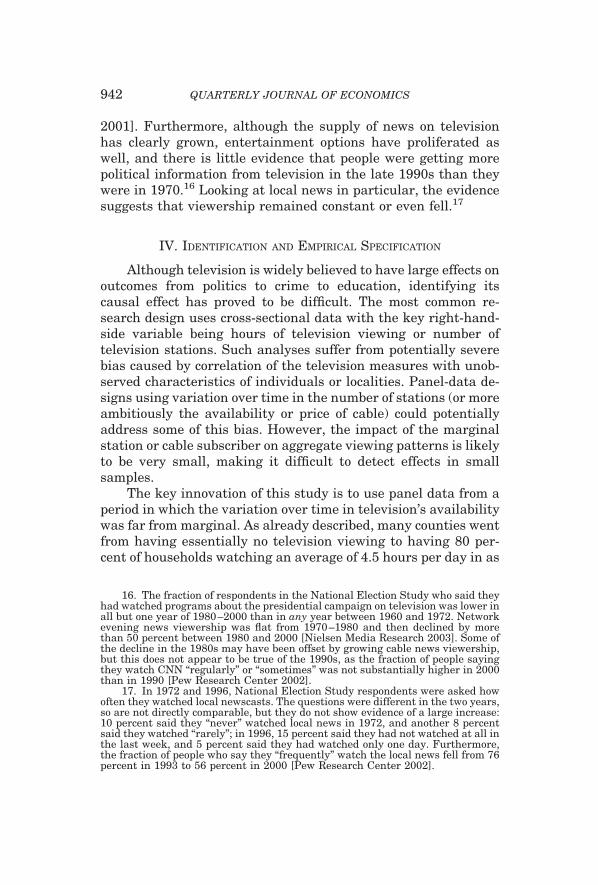
The second set of results shows that crowding out of infor-mation provides a plausible mechanism linking television andvoting. One approach is to document the extent to which televi-sion caused substitution away from newspapers and radio. Iconfirm that television news provided less political informationthan either of these other media, and that the gap was larger forinformation about congressional races. I then document the dra-matic decline in newspaper and radio use which televisioncaused. A second approach is to look directly at measures ofpolitical knowledge. I use data from the 1952 National ElectionStudy to show that respondents in counties with television wereless likely to be able to name candidates running in the election,with the strongest and most significant effects for congressionalelections. A third approach is to look for an exogenous variablethat shifts the amount of information about local congressionalraces provided by television and ask whether this also changesthe intensity of the turnout effect. The variable I consider is thenumber of congressional districts within a television market. Themore districts a market is divided into, the more congressionalraces are taking place in a given election year, and the less localstations should be able to cover any one race. Although the resultsfor the effect of districts on survey measures of information showno significant effects, the effect on turnout is exactly as predicted:having more districts increases the magnitude of television’s ef-fect in off-year congressional elections but does not change theeffect in presidential years.

These findings contribute to a growing economics literatureon the link between media and voter behavior.6 DellaVigna andKaplan [2006] study the impact of introducing the Fox Newscable channel and find a positive effect on the vote shares ofRepublican candidates, as well as evidence of a positive effect onvoter turnout. Oberholzer-Gee and Waldfogel [2001] show thatminority voter turnout is higher in counties with larger minoritypopulations, and attribute the difference to the ability of minor-ity-targeted media to deliver campaign messages. Stromberg[2004] presents evidence that penetration of radio in the New

6. I will not attempt to review the large political science literature on mediaand voter behavior. See Graber [2000] for a survey. One study of particularrelevance is Prior [2004], who uses data on television in the 1950s to argue thatit increased the incumbency advantage. A second is Althaus and Trautman[2004], who use recent cross-sectional data to show that large television marketsfragmented over many congressional districts tend to have lower turnout, espe-cially in off-year elections.


Deal period increased turnout in gubernatorial elections, an in-teresting finding that contrasts with the effect of television doc-umented here. One possible explanation is that technologicalfeatures of radio (for example, the fact that it is possible to readand listen at the same time) meant that it caused less substitu-tion away from newspapers. This is consistent with aggregatetrends in newspaper circulation per capita which show a sharpdownward trend beginning when television was introduced butno similar trend around radio’s introduction. Radio also had morepolitical coverage than television, and may have represented agreater improvement in the availability of information, especiallyin rural areas.

The remainder of the paper proceeds as follows. The nextsection discusses the construction of the data. Section III presentsbackground on the history of television’s introduction. Section IVdiscusses the paper’s identification strategy and the empiricalspecification, Section V analyzes the effect of television on turn-out, and Section VI looks at informational crowding out as apossible mechanism. Section VII concludes.

II. DATA

Data on the availability of television in each U. S. city be-tween 1940 and 1970 were compiled from various issues of Tele-vision Factbook [Television Digest 1948–1970], a yearly databook on the television industry used by advertisers, equipmentmanufacturers, station managers, and others. The books profileeach station operating in each year, giving its location, signalstrength, network affiliation, ownership, and starting date.

To define the geographic region reached by stations in aparticular city, I use Designated Market Areas (DMAs), whichare the current industry standard. Every county in the UnitedStates is assigned to one DMA such that all counties in a givenDMA have a majority of their measured viewing hours on stationsbroadcasting from that market.7 These definitions are based onviewership as of 2003, rather than in the historical period I amanalyzing. However, since the broadcasting strength of stations is

7. In a handful of cases, a county is split across multiple DMAs. (An exampleis El Dorado county in California. The eastern half of the county is assigned to theReno DMA, and the western half to the Sacramento DMA.) In these cases, I assignthe entire county to the larger of the two DMAs. Dropping these counties does notmeaningfully alter the results (see Gentzkow [2005]).


regulated by the FCC to avoid interference with neighboringmarkets, the area reached by particular stations has not changedsignificantly.8 I take the DMA definitions as a reasonable approx-imation of the viewing area of stations in the 1950s and 1960s,and calculate the first year each county received television as thefirst year in which a station in the DMA broadcast for at least fourmonths.9

One way to check the validity of the television data is tocompare the recorded entry dates to county-level television pene-tration from the 1950 and 1960 censuses. Figure I shows 1950penetration by the measured first year of television. The averagepenetration in DMAs whose first station began broadcasting be-fore 1950 ranges from 8 percent in the 1949 group to over 35percent in the 1941 group, while the average for post-1950 DMAsnever exceeds 1 percent. A similar comparison using 1960 datashows that the handful of DMAs that got television in 1960 orlater already had extensive television ownership. These DMAs

8. I have verified this by spot-checking the DMA definitions against coveragemaps from the 1960s.

9. In most cases, I use the date that a station began commercial broadcasts,as regulated by the FCC. The exceptions are two stations—KTLA in Los Angelesand WTTG in Washington, DC—that began large-scale experimental broadcastsand subsequently converted to become commercial stations. In these cases, I usethe stations’ experimental start dates.

FIGURE I1950 Television Penetration by First Television Year

Note: Years in which no county received their first station are omitted from thefigure.


are small—often consisting of only one or two counties—andcould all receive some television broadcasts from neighboringmarkets. I therefore omit all counties in DMAs whose first tele-vision station began broadcasting in 1960 or later. This applies to13 out of 205 DMAs, accounting for .7 percent of the U. S.population as of 1950. If these counties are included, the mea-sured effects of television are attenuated somewhat, but remainstatistically significant.

I combine the television data with county-level election re-turns compiled by the Inter-university Consortium for Politicaland Social Research (ICPSR).10 The data give total votes as apercentage of the legally eligible electorate, as defined by contem-porary citizenship, race, sex, and age criteria.11 This does nottake account of other eligibility criteria based on residency, orstatus as a convicted felon. Not all counties have data for allyears, and I include counties if they have turnout data availablefor a majority of the years from 1940–1972, leaving a total of 3081counties.12 I use as my key dependent measure the number ofpeople casting votes for Congress as a fraction of the eligibleelectorate.

Figures II and III plot turnout in House elections for theyears 1910–1998. Figure II shows turnout in presidential years,and Figure III in nonpresidential years. Although turnout hasbeen volatile over the century, the graphs show a marked declineafter 1960 which is steepest in the years 1960–1974 and flattensout significantly thereafter. Because there was substantial remo-bilization of Black voters in the South during this period, thedecline outside the South was even more pronounced.13

10. The study is titled “Electoral Data for Counties in the United States:Presidential and Congressional Races, 1840–1972” (ICPSR study number 8611).

11. This is the standard measure of turnout, and is considered superior to themeasure with number of registered voters in the denominator. According toPrysby [1987, p. 113]: “Calculating turnout as a proportion of registered vot-ers . . . is generally inappropriate in the American context, given the large num-bers of people who are eligible to register but fail to do so. In fact, the availableresearch indicates that most nonvoters are not registered.”

12. Rusk [2001] provides a detailed discussion of the construction of histori-cal turnout data, including possible errors in the ICPSR data. The results areunchanged if I use a balanced panel only including counties that have data for allyears.

13. Three major events that affected turnout are visible in Figures II and III.First, the Nineteenth Amendment was ratified in 1920, extending the franchise towomen. This has frequently been cited as a reason for the drop in presidentialturnout in the 1920 and 1924 elections as it took several years for voting ratesamong women to reach near-parity with those of men [Rusk 2001]. Second, therewas a sharp drop in turnout during and immediately following World War II. I


To assess political knowledge and the use of media for politi-cal information, I match the television data to the 1952 NationalElection Study.14 This is a nationally representative sample of1899 voting-age citizens interviewed both before and after the1952 election. The timing of this election is ideal, because it wasthe last year of the FCC freeze and so maximizes the idiosyncraticvariation in television access. The survey included detailed ques-tions on political attitudes, voting behavior, and demographics, aswell as limited information on media use. It also identifies thecounty of residence of each respondent.

For newspaper circulation, I compile a state-level data setusing various issues of Editor and Publisher Yearbook [Editorand Publisher 1946–1971], which give the total circulation ofdaily newspapers for each state in each year. I translate these

have not seen a convincing analysis of what caused this drop, but I wouldspeculate that it could result in part from sharply reduced participation amongmilitary personnel stationed overseas. Third, the Twenty-Sixth Amendmentpassed in 1971 required that all states extend the franchise to 18–21-year-olds, agroup that historically has significantly lower turnout rates than older voters.Kleppner [1982, p. 123] estimates that approximately 25 percent of the drop inturnout between 1968 and 1972 can be attributed to the expanding electorate.

14. The study is titled “American National Election Study, 1952” (ICPSRstudy number 7213).

FIGURE IICongressional Turnout in Presidential Election Years


into circulation per capita using census population data. Countyand city-level demographics are obtained from the decennial cen-sus, with intercensus years estimated by linear interpolation.

III. THE INTRODUCTION AND GROWTH OF TELEVISION

Television technology was already well developed by the late1930s. The first workable prototypes for television receivers weremade in the early 1920s, the first public demonstration took placein 1923, and numerous experimental broadcasts were made inthe late 1920s. By 1931, eighteen experimental stations wereoperating in four cities. The first television sets went on sale in1938, and by 1939 fourteen companies were offering sets for sale.After several delays, the Federal Communications Commission(FCC) finally licensed television for full-scale commercial broad-casting on July 1, 1941.15

Although television seemed poised for rapid growth at thispoint, two events intervened to delay the process. The first wasWorld War II: less than a year after the FCC authorization, the

15. This section draws primarily on Sterling and Kittross [2001] and Bar-nouw [1990]. For details on the regulatory process, see also Slotten [2000].

FIGURE IIICongressional Turnout in Nonpresidential Years


government issued a ban on new television station construction topreserve materials for the war effort. Although existing stationscontinued to broadcast, the total number of sets in use during thewar was less than 20,000. After the war, television grew rapidly.Over 100 new licenses were issued between 1946 and 1948, sothat by 1950 half of the country’s population was reached bytelevision signals. This growth was again halted, however, by anFCC-imposed freeze on new television licenses in September1948. The FCC had determined that spectrum allocations did notleave sufficient space between adjacent markets, causing exces-sive interference. The process of redesigning the spectrum allo-cation took several years, and it was not until April 1952 that theFCC lifted the freeze and began issuing new licenses.

To justify the empirical analysis that follows, it is importantto establish that the diffusion of television was rapid enough thatits effects could be felt within a relatively short window of time.One reason is that many aspects of the television industry—fromthe format of newscasts, to the structure of the networks—hadbeen developed and perfected by the radio industry. Also, thetechnical and logistical aspects of television had been largelyworked out well before the end of the war. A number of techno-logical innovations during the war years, including better cam-eras and a technology for rebroadcasting cinema film, furtherimproved quality. As Barnouw [1990] writes, the prospects fortelevision’s growth after the war were “explosive”:

Electronic assembly lines, freed from production of electronic war materiel,were ready to turn out picture tubes and television sets. Consumers, longconfronted by wartime shortages and rationing, had accumulated savingsand were ready to buy. Manufacturers of many kinds, ready to switch fromarmaments back to consumer goods, were eager to advertise [p. 99].

We can look at the pattern of television’s growth in a numberof different ways. Some evidence was presented in Figure I, whichshowed substantial diffusion of television ownership by 1950 (13percent on average in markets that had television). Figure IVshows the time path of diffusion, drawing on data from Nielsensurveys. In the largest counties, 20 percent had televisions by1950, and 80 percent had televisions by 1955. Data from Nielsensurveys also show that in those households with television, view-ership had already surpassed four and a half hours per day by1950 [Television Bureau of Advertising 2003].

Though the most dramatic period of growth in stations and


ownership occurred between 1950 and 1960, growth continuedafter 1960 on other dimensions. Although the number of house-holds with televisions had plateaued, the number with multiplesets more than tripled between 1960 and 1970 [Sterling 1984, p.236]. Color television was introduced at the end of the 1950s, andthe fraction of television households with color sets increasedfrom less than 1 percent in 1960 to more than 50 percent in 1972[Television Digest 2001]. The combined effect of these changes isreflected in the number of viewing hours per household, whichincreased from four and a half hours in 1950, to just over fivehours in 1960, to more than six hours by 1975.

While the analysis in this paper does not extend beyond1970, it is worth examining briefly how television has changedsince then. If the scale of television continued to increase, thelong-run effects could be even greater than those documentedhere. On the other hand, if television began providing substan-tially more political information, some of the effects could actu-ally be reversed. In reality, the former seems more likely than thelatter. The time devoted to television viewing continued to in-crease steadily until the mid-1980s, with daily viewership in 199550 percent higher than in 1965 [Robinson and Godbey 1999]. Thenumber of sets per household increased from 1.4 to 2.3 between1970 and 1995 [Putnam 2000], and both color television and cablesaw the majority of their growth after 1970 [Television Digest

FIGURE IVPercent of U. S. Households with Television by County Size

Note: Data are from Nielsen Television Index as quoted in Sterling [1984]. “ACounties” are all counties in the 25 largest metropolitan areas. “B Counties” areall counties not in A with populations of over 150,000 or in metropolitan areas.


2001]. Furthermore, although the supply of news on televisionhas clearly grown, entertainment options have proliferated aswell, and there is little evidence that people were getting morepolitical information from television in the late 1990s than theywere in 1970.16 Looking at local news in particular, the evidencesuggests that viewership remained constant or even fell.17

IV. IDENTIFICATION AND EMPIRICAL SPECIFICATION

Although television is widely believed to have large effects onoutcomes from politics to crime to education, identifying itscausal effect has proved to be difficult. The most common re-search design uses cross-sectional data with the key right-hand-side variable being hours of television viewing or number oftelevision stations. Such analyses suffer from potentially severebias caused by correlation of the television measures with unob-served characteristics of individuals or localities. Panel-data de-signs using variation over time in the number of stations (or moreambitiously the availability or price of cable) could potentiallyaddress some of this bias. However, the impact of the marginalstation or cable subscriber on aggregate viewing patterns is likelyto be very small, making it difficult to detect effects in smallsamples.

The key innovation of this study is to use panel data from aperiod in which the variation over time in television’s availabilitywas far from marginal. As already described, many counties wentfrom having essentially no television viewing to having 80 per-cent of households watching an average of 4.5 hours per day in as

16. The fraction of respondents in the National Election Study who said theyhad watched programs about the presidential campaign on television was lower inall but one year of 1980–2000 than in any year between 1960 and 1972. Networkevening news viewership was flat from 1970–1980 and then declined by morethan 50 percent between 1980 and 2000 [Nielsen Media Research 2003]. Some ofthe decline in the 1980s may have been offset by growing cable news viewership,but this does not appear to be true of the 1990s, as the fraction of people sayingthey watch CNN “regularly” or “sometimes” was not substantially higher in 2000than in 1990 [Pew Research Center 2002].

17. In 1972 and 1996, National Election Study respondents were asked howoften they watched local newscasts. The questions were different in the two years,so are not directly comparable, but they do not show evidence of a large increase:10 percent said they “never” watched local news in 1972, and another 8 percentsaid they watched “rarely”; in 1996, 15 percent said they had not watched at all inthe last week, and 5 percent said they had watched only one day. Furthermore,the fraction of people who say they “frequently” watch the local news fell from 76percent in 1993 to 56 percent in 2000 [Pew Research Center 2002].


little as five years. Furthermore, the last significant group ofcounties to receive television got it a full ten years after thepostwar growth of television began in the largest cities. Thissuggests a differences-in-differences research design that askswhether changes in political information or voter turnout werecorrelated with the timing of television’s introduction.

Two key features of the data allow me to strengthen thisbasic identification strategy. The first is the fact that both WorldWar II and the FCC freeze were exogenous shocks to the patternof television’s introduction across markets. The second is the factthat individual television stations broadcast over a large area,reaching a heterogeneous group of counties.

To examine the first of these, Figure V shows the fraction of theU. S. population in counties receiving television for the first time ineach year. Three distinct groupings are clearly visible: counties thathad television before the war, starting in 1940; counties that gottelevision between 1945 and 1951, with the bulk in 1948 and 1949;and counties that got their first station after the freeze, beginning in1952. The gaps between these three groups are much greater thanthey would have been if exogenous events had not intervened, andthis added variation adds identification power.

While the war and the freeze changed the timing of televi-sion’s introduction across markets, they did not necessarilychange the ordering. Predictably, it was in the largest andwealthiest television markets that potential entrants found it

FIGURE V1950 Population of Counties by Year Television Was Introduced


profitable to apply for licenses and begin broadcasting in theearliest years. Table I shows county-level demographics for thethree major groupings of counties: counties that got televisionearlier were larger, more urban, with higher income, median age,and schooling; the earliest group also had substantially higherturnout in the 1940 election. Although the panel design controlsfor both cross-sectional differences correlated with the timing oftelevision’s introduction and common changes over time, the re-sults could still be biased if there were negative shocks to infor-mation or voting that hit the largest and richest cities in themid-1940s, medium-sized cities in the late-1940s, and small citiesand rural areas in the early-1950s.

One way to address this issue is to make use of observablecounty characteristics. Note, for example, that the largest differ-ences in observables shown in Table I are between the first twogroups; the only large differences between the 1945–1951 andpostfreeze groups are in population, population density, and per-cent urban. This suggests that spurious correlation is likely to be

TABLE ISUMMARY STATISTICS

Mean St. dev.

Mean by year of first TV station

1940–1944 1945–1951 1952 and later

Percent urban(1950) 29.0 27.1 60.4 31.6 26.0

Population (1960’000) 59,428 208,549 466,960 76,057 31,278

Income per capita(1959) $1,352 405 $2,044 $1,391 $1,298

% high school(1950) 27.2 10.9 35.9 27.0 26.8

Median age (1950) 28.5 3.92 32.8 28.7 28.1Percent non-White

(1950) 10.9 17.0 4.48 10.1 11.7Persons per square

mile (1950) 209 2,077 3,006 235 67.5Base year turnout

(1940) 56.5 23.6 73.1 57.4 55.2N 2958 83 1052 1823

Percent high school is the fraction of the population aged 25 and older who completed high school. Incomeper capita is measured in 1959 dollars.


less of a problem if attention is restricted to the latter groups.18

Furthermore, a simple regression analysis confirms that marketsize and income were the key determinants of the timing oftelevision’s introduction. A linear regression at the DMA level ofthe year television was introduced on log population and log totalincome yields an R2 of .69. When the residuals from this regres-sion are regressed on percent urban, percent high school, medianage, percent non-White, population density, median income, and1940 turnout, the coefficients are neither individually nor jointlysignificant at the 10 percent level. The largest individual t-sta-tistics are on percent urban, percent non-White, and populationdensity (�1.46, �1.17, and �1.04, respectively). This suggeststhat controls for population and income may eliminate much ofthe spurious correlation.

An even more powerful way to address this issue is to exploitthe large and heterogeneous broadcast area of individual televi-sion stations. Consider Figure VI which shows a map of theChicago DMA and the characteristics of the counties that com-pose it. Although Chicago was the second largest television mar-ket in 1950 and the DMA as a whole is highly urban, dense, andwealthy, the counties that compose it are heterogeneous. Theyrange from Newton County, IN, which has no urban population,a density of 27 people per square mile, and a median income (in1950 dollars) of $2,778, to Cook County, IL, which has 99 percenturban population, a density of 4726 people per square mile, and amedian income of $4,085. If there were bias in the basic panelspecification caused by shocks to voting in dense urban areas inthe mid-1940s, this should show up in the voting patterns of CookCounty but not Newton County. A robust way to identify televi-sion’s effect would therefore be to compare counties that aresimilar on dimensions like density and percent urban (takingonly rural counties like Newton, for example) and ask whetherthey saw changes in voting around the time television was intro-duced. The variation in the timing of television would then bedriven by whether a county happened to fall within the roughly100-mile radius of television broadcasts from a large city, withthe identifying assumption being that proximity at this distanceis uncorrelated with unobserved shocks that changed the level ofturnout over time.

18. Gentzkow [2005] verifies that the results are robust to excluding theearliest television counties.


The basic framework for the analysis is a fixed effects regres-sion of the form,

(1) Yit � �i � �rt � �TVit � �Xit � �it,

where i indexes counties, t indexes years, and r indexes censusregions. Yit is an outcome measure of interest, �i and �rt arelocation and region-time fixed effects, respectively, and �it is arandom shock. TVit is some measure of the scale of television in

FIGURE VIThe Chicago DMA


county i and time t. Xit includes observable county characteris-tics (that change over time) and other functions of these charac-teristics described below. It also includes the absolute differenceof the Republican and Democratic vote percentages, a competi-tiveness measure that has been shown to have a strong effect onturnout (see Stromberg 2004). Note that in specifications usingthe National Election Study data, the variation is only cross-sectional, and so I cannot include the �i and �rt terms in equation(1).

I use two approaches to exploit within-DMA heterogeneity.The first is to include in Xit interactions between key county-levelobservables in a base year and a fourth-order polynomial in time.This controls flexibly for differences in the time path of thedependent variables whose correlation with television is drivenby the endogenous pattern of television’s introduction. Based onthe analysis of this timing described above, I include interactionswith 1960 log population, 1959 log total income, and turnout inthe 1940 election.19 I also check that the results are robust toincluding interactions with 1950 percent urban, 1950 populationdensity, and 1950 percent non-White, the remaining characteris-tics with t-statistics greater than one in the timing regression.The second approach is to partition the counties into thirds alongobservable dimensions and run the analysis separately for eachgroup. This more flexible specification allows the region-timedummies to be estimated separately for each group. It is also aliteral implementation of the experiment described above—com-paring similar counties that differ in the timing of televisionbecause of their proximity to large cities.20

The remaining issue is how to model the effect of television.

19. I also include an interaction of the time polynomial with a dummyvariable indicating a missing value for 1940 turnout. Turnout in 1940 is notsignificantly related to the year television was introduced once population andincome are controlled for, but since any residual correlation could lead to severebias it seems safest to include it.

20. A third way to exploit within-DMA heterogeneity would be to use amatching algorithm. As a robustness check, I have estimated the effect of televi-sion using the nearest-neighbor matching algorithm of Abadie and Imbens [2004].I define a binary treatment variable equal to one if a county received televisionbefore the end of the FCC freeze (1952), and two dependent variables: the changein turnout between the presidential elections of 1944 and 1952; and the change inturnout between the off-year elections of 1946 and 1954. I match counties basedon 1960 log population and log per capita income and 1950 median age, populationdensity, percent urban, percent non-White, percent with high-school diploma, andmedian income. I consider specifications with and without bias correction, withbetween one and four matched observations, and with heteroskedasticity-cor-rected standard errors. The sample average treatment effect of television is


There are several reasons to expect that its impact would not bea one-time discontinuous change, but would rather grow gradu-ally over time. The quantity and quality of programming in-creased steadily following television’s initial introduction, televi-sion ownership diffused slowly across households, and the processby which television is linked to voting—substitution among me-dia leading to a depreciating stock of information and ultimatelyto reduced participation in elections—would be expected to takeeffect gradually over time.

A natural starting point, then, would be to allow TVit to growlinearly over time, beginning in the year when the first stationstarts broadcasting in county i. That is, TVit � I(t � i)(t � i),where i is the year television is introduced and I( ) is theindicator function. Because penetration of television was negligi-ble before the end of World War II, I assign a first television yearor 1946 to all counties that had stations before that date. I alsoinclude separate trends for presidential and off-year elections. Insome specifications I also include the squared value of TVit toallow the effect to grow weaker over time.

To further check the validity of the identification strategy,Table II presents results from a series of placebo regressions. Thegoal is to test whether once the effect of the key observables ispartialed out, variation in the timing of television’s introductionis orthogonal to the remaining observables. The timing of televi-sion is measured by a dummy equal to one if a county receivedtheir first station after the FCC freeze.21 Column 1 of the tabledisplays the F-statistic for the null hypothesis that the coeffi-cients on the remaining observables are all equal to zero. Column2 shows the number of the coefficients that are individuallysignificant at the 5 percent level.

The first set of tests looks at whether the timing of televisionis orthogonal to the full vector of observables once we restrictattention to subsets of counties. The F-statistics here are from asimple regression of the postfreeze dummy on the eight demo-

significant at the .1 percent level in all specifications, and roughly 50 percentlarger for off-year turnout than for presidential-year turnout.

21. An alternative is to use the year television was introduced as the left-hand variable. In this case, the F-statistic for the lowest third by populationdensity is no longer significant, while the F-statistic for the whole sample regres-sion becomes significant at the 1 percent level.


graphics shown in Table I and region dummies.22 For the lowestthird of counties by population, income per capita, and 1940turnout, the hypothesis that the demographic coefficients arejointly equal to zero cannot be rejected. It is rejected at the 5percent level for the lowest third by density and percent with highschool education, and at the 1 percent level for the lowest third bypercent urban. In no case is more than one demographic coeffi-cient individually significant. This suggests that focusing on sub-sets of counties removes much, but possibly not all, correlationbetween the timing of television and county characteristics.

The next test looks at whether the timing of television is

22. Because the subset regressions below allow a different set of time dum-mies by region, the region dummies are treated as incidental controls here and notincluded in the F-test.

TABLE IIPLACEBO REGRESSIONS WITH POSTFREEZE DUMMY AS DEPENDENT VARIABLE

(F-test for joint significance of demographics)

F# Significantcoefficients

Lowest third of counties by:Population (1960 ’000) 1.32 0 of 8Population per square mile (1950) 2.23* 1 of 8Percent urban (1950) 4.38** 1 of 8Income per capita (1959) 1.50 0 of 8% high school (1950) 2.29* 1 of 81940 turnout 1.92 1 of 8

Full sample after controlling for logpopulation, log income, and 1940turnout 1.04 0 of 5

National Election Study sample 1.31 1 of 28

* Significant at the 5 percent level.** Significant at the 1 percent level.The two columns show F-statistics for the joint significance of the demographic variables in each

regression and the number of coefficients significant at the 5 percent level, respectively. The “lowest third ofcounties” regressions use only counties falling into the lowest third of the indicated demographics; thedependent variable is a dummy equal to one if television was introduced in 1952 or later and the right-hand-side variables are log total income, log population, percent urban, percent non-White, percent high school,median age, population density, and 1940 turnout; region dummies are also included but not reported in theF-test. In the “full sample” regression, the dependent variable is the residual from a regression of thepostfreeze dummy on log population, log total income, 1940 turnout, and region dummies; the right-handvariables are percent urban, percent non-White, percent high school, median age, and population density. Inthe “National Election Study” regression, the dependent variable is the residual from a regression of a dummyfor having TV in 1952 on DMA log population and log total income, county percent non-White, and regiondummies; the right-hand side variables are individual-level dummies for male, White, age categories,education categories, occupation categories, income in the highest category, and missing values, as well asnumber of children and log income.


orthogonal to observables in the full sample once we control forpopulation, income, 1940 turnout, and region dummies (the vari-ables that are interacted with a time polynomial in the mainspecification). In a regression of these residuals on the remainingdemographics, the demographics are neither jointly nor individ-ually significant, confirming that the remaining variation islargely idiosyncratic.

The final test looks at the orthogonality of television in theNational Election Study sample. Here, the data are at the indi-vidual level, and the dependent variable is a dummy equal to oneif the respondent’s county had television in 1952. The specifica-tion tests whether individual respondent characteristics predicthaving television once region dummies and county-level popula-tion, income, and percent non-White are controlled for. The 28right-hand variables are neither jointly nor individually signifi-cant, again confirming that the remaining variation in timing isidiosyncratic.

V. DID TELEVISION AFFECT TURNOUT?

V.A. Relative Trends

As a first step in analyzing the effect of television on turnout,I present direct comparisons of turnout in counties divided intothree groups by the year their first television station began broad-casting. This is a coarser approach than will be possible with thefixed effects model of equation (1), but has the advantage ofallowing one to look at the data directly.

As was clear from Figure V, the natural groups are pre-1945,1945–1951, and 1952 and after. If television reduced voter turn-out, we would expect the first two groups to show a negative trendrelative to the third group in the years up to 1952. The relativedecline should begin in 1946 for the first group (recall that tele-vision did not begin to diffuse widely until after the war), andsometime between 1946 and 1948 for the second group.

Figure VII shows turnout in the first and second groups,respectively, measured relative to the third. To construct thefigure, I regress county-level turnout on year-region dummies (Itake out separate time effects by region to control for the exoge-nous changes affecting turnout in the South). I then calculate themean of the residuals for each group in each year. The first panelplots the mean of the first group residuals minus the mean of the


third. The second panel plots the mean of the second groupresiduals minus the mean of the third.

A clear relative decline is apparent for both groups, begin-ning in 1946. That the negative trend is slightly larger for the

FIGURE VIIVoter Turnout by Year of Television’s Introduction

(Relative to Post-1951 Counties)


first group is consistent with the early areas having relativelyhigh income and density and thus being the places where televi-sion ownership diffused the fastest (a point which is examinedmore rigorously when I add interaction terms to the regressionanalysis). For the first group, the relative trend also clearly flat-tens out beginning in 1954, the year that most counties in thereference group first had television. No clear flattening is visiblefor the second group.

Table III provides a more detailed look at these trends in aregression framework. I regress county-level congressional turn-out on differential trends for the first two television groups rela-tive to the third for both the pre-1952 and post-1952 periods.23

23. More precisely, TVit is specified as four separate terms: an interaction ofa dummy for membership in the first group and a time trend for the years1944–1950; an interaction of the first group dummy and a trend for 1952; an

TABLE IIIDIFFERENTIAL TRENDS IN VOTER TURNOUT BY YEAR OF TELEVISION’S INTRODUCTION

(Relative to counties where television was introduced in 1952 or later)

(1) (2) (3)

First year of TV before 1945Relative trend, 1944–1950 �.513 �.414 �.399

(.0775) (.0777) (.0750)Relative trend, 1952 �.306 �.006 .026

(.0618) (.0542) (.0535)First year of TV 1945–1951

Relative trend, 1946–1950 �.125 �.101 �.106(.0391) (.0396) (.0386)

Relative trend, 1952 �.139 �.030 �.0219(.0241) (.0192) (.0194)

Demographics XTime polynomial interactions X XCounty, year-region dummies: X X XR2 .914 .925 .927N 46003 46003 46003

Standard errors are clustered by county. Dependent variable is the percentage of legally eligible voterscasting a vote for Congress. All trends are relative to counties getting television in 1952 or later. When yearsare given for a relative trend (e.g., 1944–1950), the coefficient is on a variable equal to zero in the first year(1944), one in the second year (1945), and so forth. All regressions include county fixed effects, separate yearfixed effects by census region, the absolute difference between the Democrat and Republican vote percent-ages, and a dummy for a missing value for the absolute difference. Demographics are log population,population density, percent urban, percent non-White, median income, median age, and percent withhigh-school education. Time polynomial interactions are a fourth-order polynomial in time interacted with1960 log population, 1959 log total income, 1940 congressional turnout, and an indicator for a missing valueof 1940 congressional turnout. Note that the levels of these variables are absorbed by the county fixed effects.


Observe that in the simple model where all counties have anidentical linear television effect, the coefficients would be nega-tive for both groups in the earlier period and zero thereafter. Thefirst column duplicates what was shown in Figure VII, includingonly county and year-region fixed effects. The second adds inter-actions of county 1960 log population, 1959 log total income, and1940 turnout with a fourth-order polynomial in time. Note thatthe levels of these variables are absorbed in the county fixedeffects. The third adds levels of log population, population persquare mile, percent urban, percent non-White, median income,median age, and percent with high-school education. The resultsshow that the negative relative trend in early television countiesis robust to the inclusion of controls, and that it flattens outsignificantly once the later counties also have television(post-1952).

V.B. Years of Television Regressions

Table IV presents the core set of regressions in this section.These are again based on equation (1) but differ from the relativetrends regression in that rather than using a coarse division ofcounties into three groups and looking at the first two groupsrelative to the third, the TVit variable is defined as a separatetrend for each county beginning in the year it first receivedtelevision. That is, TVit � I(t � i)(t � i), where i is the yeartelevision was introduced in county i and I( ) is the indicatorfunction. The first two columns show the coefficients on thisvariable in specifications with county and region-year dummiesalone, and then adding time polynomial interactions and demo-graphics. The results show that television caused a significantdecline in voter turnout. The magnitude of this effect drops withthe added controls but remains strongly significant. In the com-plete specification, introducing television causes turnout to fall by.136 percentage points per year.

The next two columns repeat these specifications allowingdifferent trends for presidential and off-year congressional elec-tions. The off-year coefficient is significantly negative and sug-gests that television reduced turnout by .196 percentage pointsper year in the specification with controls. For presidential years,

interaction of a second group dummy and a trend for 1946–1950; and an inter-action of a second group dummy and a trend for 1952.


on the other hand, the coefficient is significantly negative in thesimplest specification, but it is much smaller and insignificantwith the full set of controls. In the final specification, the pointestimate is a negative effect of .067 percentage points per year.The final three columns add additional interactions between thetime polynomial and percent urban, population density, and per-cent non-White, respectively. These were the three characteris-tics, after those already included in the interactions, that had thehighest t-statistics in the DMA-level regression of television’stiming on demographics (though none were significant). The re-sults do not change substantially when these interactions areincluded, suggesting that the remaining variation identifying thetelevision coefficient is largely idiosyncratic.

The results presented so far cast doubt on the hypothesisthat the apparent effect of television is driven by spurious corre-lation with some unrelated shock to voting. The effect remainsstrong and significant in a variety of specifications even afterallowing interactions between a flexible function of time and all ofthe major correlates of the timing of television’s introduction.This means in particular that any factor influencing voting whose

TABLE IVREGRESSIONS OF TURNOUT ON YEARS OF TELEVISION

(1) (2) (3) (4) (5) (6) (7)

Years of TV �.416 �.136(.0486) (.0412)

Years of TV � nonpresidential �.489 �.196 �.193 �.187 �.188year (.0577) (.0478) (.0483) (.0478) (.0477)

Years of TV � presidential �.332 �.067 �.067 �.059 �.056year (.0468) (.0438) (.0443) (.0437) (.0434)

Additional time-polynomialinteractions:Time � percent urban XTime � population density XTime � percent non-White X

Demographics X X X X XTime polynomial interactions X X X X XCounty, year-region dummies: X X X X X X XR2 .913 .927 .913 .927 .927 .927 .927N 46003 46003 46003 46003 46003 46003 46003

Standard errors are clustered by county. Years of TV is the number of years since the first year in whicha commercial station was broadcasting in the county for at least three months. The dependent variable is thepercentage of legally eligible voters casting votes for congress. Fixed effects, demographics, and timepolynomial interactions are as in Table III. All regressions include the absolute difference between theDemocratic and Republican vote percentage. Additional time-polynomial interactions are interactions of afourth-degree polynomial in time with the indicated demographics.


correlation with television was driven by city size or income—forexample, a social change that began in the largest cities in the1940s and then diffused outward—would not bias the coefficients.

It is possible to perform an even stronger check on the valid-ity of the results. As discussed earlier, a more direct way toexploit the fact that television stations broadcast to a heteroge-neous group of counties is to perform the analysis using onlythose that are demographically similar—for example, comparingturnout patterns in rural counties that happened to get televisionearly because of proximity to a large city and those that gottelevision late. In Table V, I divide counties into thirds by differ-ent observable characteristics and then perform the analysisseparately on each third. The table reports the coefficient onyears of television from a regression of turnout on this variable,county dummies, and separate year dummies by region (as wellas the usual competitiveness measure). The first column of thefirst row, for example, reports this coefficient using only thesmallest counties.

The results provide further evidence that the estimates rep-

TABLE VREGRESSIONS OF TURNOUT ON YEARS OF TELEVISION FOR SUBSETS OF COUNTIES

(Coefficient on years of television)

Lowest third Second third Highest third

Counties partitioned by:Population �.332** �.228** �.443**

(.1045) (.0798) (.0819)Population density �.447** �.239** �.289**

(.1041) (.0798) (.0827)Percent urban �.380** �.296** �.440**

(.0940) (.0885) (.0733)Per capita income �.127 �.228** �.578**

(.0984) (.0803) (.0817)% high school �.275** �.282** �.706**

(.0940) (.0798) (.0752)1940 turnout �.160* �.365** �.518**

(.0778) (.0788) (.0781)

* Significant at the 5 percent level.** Significant at the 1 percent level.Standard errors are clustered by county. The table shows the coefficient on years of TV from regressions

of turnout on the absolute difference between the Democrat and Republican vote percentages, countydummies, and year-region dummies. The years of TV variable is as in Table IV. Each column gives thecoefficient from regressions using only counties that fell into the given third of the data, and each rowspecifies the demographic characteristic on which counties were divided.


resent a causal effect of television. The television coefficient re-mains significant in all but one of the eighteen specifications, andhas the correct sign in all of them. The magnitude does not varyin a systematic way across thirds by population or percent urban,and is actually largest in the least dense counties, providingstrong evidence against the hypothesis that the results are drivenby changes taking place in the largest cities. (Note that even ifthere were shocks to large cities that reverberated throughout thebroader television markets, we would expect the coefficients to besmaller for the less urban counties.) On the other hand, themagnitude is higher in quartiles with higher levels of income andeducation, consistent with the expectation that these would bethe counties where television diffused the fastest. Finally, theeffect is larger for counties whose turnout at the beginning of theperiod was highest. One interpretation is that the voting popula-tion in these counties in 1940 included a large number of rela-tively marginal voters whose turnout was more affected by theintroduction of television.

V.C. Interactions and Nonlinear Effects

The next step in the analysis is to look in more detail at theway the magnitude of the television effect varies with countycharacteristics. The most obvious reason that the effect mightdiffer is because television ownership (and in later years mul-tiple set and color ownership) diffused faster and more broadlyin some places than others. The picture is more complicated,however, because we would also expect the sensitivity of turn-out to a given change in information consumption to vary withdemographics. For example, if wealthier or more educatedindividuals have high levels of information regardless of mediaconsumption, they would tend to be farther away from theturnout margin, and less affected by the introduction oftelevision.

To structure the analysis of the interactions, I construct twovectors of fitted values: predicted television diffusion and pre-dicted turnout sensitivity. The first is based on a regression of1960 television penetration on the census year demographicsfrom Table I and dummy variables for the year in which televi-sion was introduced. The fitted values are from the demographicsalone. The second is derived by asking how sensitivity to thecloseness of elections varies across counties. Although there is noreason to expect the reaction to variation in election closeness to


be identical to the reaction to information, we would expect thatcounties that had a large number of marginal voters would re-spond more to both. I regress turnout on county fixed effects,time-region fixed effects, the absolute difference in Republicanand Democratic vote shares, and interactions of the absolutedifference with the census-year demographics from Table I and1940 turnout.24 The fitted values are the predicted marginaleffect of the absolute difference in vote shares.25

Table VI presents turnout regressions that allow a heteroge-neous effect of television. The first column includes interactionswith the full set of county demographics. The negative trendintroduced by television is larger in counties with low population,high income, low education, high percent non-White, high den-sity, and high 1940 turnout. These results are hard to interpretbecause they may conflate differences in the diffusion of televi-sion and the fraction of marginal voters. Column (2) includes aninteraction with predicted television penetration in 1960 andshows that the television effect is largest in those counties whereownership diffused the fastest. The effect is large, with a onestandard deviation increase in diffusion more than doubling thetelevision effect. Column (3) includes an interaction with thepredicted sensitivity of turnout and shows that the televisioneffect is largest where the fraction of marginal voters is highest.A one standard deviation increase in this variable increases thetelevision effect by approximately 60 percent. Column (4) in-cludes both the diffusion and sensitivity measures. The magni-tude of the former falls slightly, and the magnitude of the latterincreases slightly. Both remain highly significant. Column (5)adds an interaction with the year television was introduced,which is small and insignificant.

The last three columns of Table VI address the question ofhow the effect of television changes over time by including bothyears of television and years of television squared. One weaknessof a research design that relies on relative changes betweencounties over time is that such nonlinearities will be difficult toseparate from heterogeneity across counties. Recall, for example,

24. County turnout in 1940 is allowed to affect sensitivity but not diffusion—this is based on the assumption that unusually high turnout may reflect theparticipation of a large block of marginal voters but should not directly affecttelevision set purchases.

25. See Gentzkow [2005] for more detailed discussion of the construction ofthese predicted values.


TA

BL

EV

IIN

TE

RA

CT

ION

SA

ND

NO

NL

INE

AR

EF

FE

CT

S

(1)

(2)

(3)

(4)

(5)

(6)

(7)

(8)

Yea

rsof

TV

�.1

28�

.123

�.1

38�

.114

�.1

99�

.186

�.1

60�

.192

(.04

22)

(.04

13)

(.04

21)

(.04

25)

(.05

28)

(.04

89)

(.05

22)

(.05

43)

Yea

rsof

TV

squ

ared

.002

35.0

255

.010

4(.

0020

5)(.

0125

)(.

0126

)In

tera

ctio

nw

ith

:P

redi

cted

diff

usi

on�

.018

4�

.016

8�

.017

1�

.016

7(m

ean

�0,

std

ev�

8.76

)(.

0036

7)(.

0036

5)(.

0036

7)(.

0037

4)P

redi

cted

sen

siti

vity

�.0

828

�.1

08�

.111

�.1

10(m

ean

�0,

std

ev�

1)(.

0138

)(.

0147

)(.

0149

)(.

0150

)F

irst

TV

year

�.0

0761

.046

6.0

1281

(mea

n�

0,st

dev

�2.

58)

(.00

419)

(.02

52)

(.02

56)

Per

cen

tu

rban

(195

0)�

.000

337

(.00

0476

)L

ogpo

pula

tion

(196

0).1

31(.

0394

)L

ogin

com

epe

rca

pita

(195

9)�

.360

(.19

2)%

hig

hsc

hoo

l(1

950)

.003

72(.

0014

5)M

edia

nag

e(1

950)

�.0

236

(.00

286)

Per

cen

tn

on-W

hit

e(1

950)

�.0

0264

(.00

0968

)P

opu

lati

onde

nsi

ty(1

950)

�.0

123

(.00

278)

1940

turn

out

�.0

0380

(.00

194)

Dem

ogra

phic

sX

XX

XX

XX

XT

ime

poly

nom

ial

inte

ract

ion

sX

XX

XX

XX

XC

oun

ty,

year

-reg

ion

du

mm

ies:

XX

XX

XX

XX

R2

.927

3.9

270

.926

9.9

270

.927

1.9

268

.926

8.9

271

N42

832

4600

342

832

4283

242

832

4600

346

003

4283

2

Sta

nda

rder

rors

are

clu

ster

edby

cou

nty

.Th

ede

pen

den

tva

riab

le,fi

xed

effe

cts,

dem

ogra

phic

s,an

dti

me

poly

nom

ial

inte

ract

ion

sar

eas

inT

able

III.

Th

eY

ears

ofT

Vva

riab

leis

asin

Tab

leIV

.A

llre

gres

sion

sin

clu

deth

eab

solu

tedi

ffer

ence

betw

een

the

Dem

ocra

tan

dR

epu

blic

anvo

tepe

rcen

tage

.A

llin

tera

ctio

ns

are

the

Yea

rsof

TV

vari

able

tim

esth

ein

tera

ctio

nva

riab

lem

inu

sit

sm

ean

.Pre

dict

eddi

ffu

sion

and

pred

icte

dse

nsi

tivi

tyar

efi

tted

valu

esfr

omre

gres

sion

sof

diff

usi

onan

dtu

rnou

tse

nsi

tivi

tyon

dem

ogra

phic

sas

desc

ribe

din

the

text

.


that the relative trend regressions in Table III show that turnoutin the early television counties neither rises or falls relative to thelater counties after 1952 (when all counties have television). Thiscould reflect a constant linear television effect whose magnitudeis the same across counties. Alternatively, it could reflect an effectthat gets smaller over time combined with a smaller effect overallfor the later counties. The results in columns (6) through (8) showthat the estimated quadratic term is highly sensitive to whichinteraction terms are included. It is positive in all specifications(suggesting that the effect is getting smaller over time), but it isonly significant in the regression with only the first TV yearinteraction. The magnitude ranges from .002 (implying that itwould take 93 years for the effect to die out entirely) to .0255(implying that this would take only 6 years). This suggests thatthere is some nonlinearity, but that the exact functional form isbeyond the power of these data to identify convincingly. It alsosuggests that estimates of the total impact of television over along period of time are unlikely to be very precise.

V.D. Magnitudes

We can evaluate the magnitude of the effects documentedabove in a number of ways. The main specifications in Table IVimply that television decreased off-year turnout by approximately2 percent each decade after it was introduced. They imply that itdecreased presidential turnout by .7 percent, although this esti-mate is not significantly different from zero. As context for thesenumbers, the overall negative trend in non-South turnout sincethe 1950s was 3.4 percent per decade, and the negative trend inpresidential turnout was 3.2 percent per decade, implying thattelevision accounted for 60 percent of the off-year decline and(possibly) 22 percent of the presidential decline. Although theseeffects assume that the per-year decline in voting remains con-stant over time, and so might overstate how much of the declinetelevision explains, they probably do not do so by much becausemost of the aggregate decline took place before 1970.

To more accurately assess the effect on overall turnout, it isnecessary to take account of the fact that television was intro-duced to different counties at different times and that the effectwas larger in some counties than others. To do so, I estimatecounterfactual aggregate turnout levels based on the estimatedparameters. The preferred specification is the nonlinear model incolumn (8) of Table VI to which I add separate television effects


for presidential and off years—this allows both a squared term inyears of television and a full set of interactions. I also check theresults for the basic specification in column (3) of Table IV and thespecification with interaction terms only in column (5) of TableVI, again allowing for a separate presidential year effect. Foreach model, I ask how much higher turnout would have been iftelevision had never been introduced assuming that televisioncaused no further effect after 1970. As a point of reference forthese results, the difference between the average non-South turn-out level in the 1950s and in the 1980s–1990s was 11 percentagepoints for off-year elections and 13 points for presidential elec-tions. The difference between the highest and lowest turnoutyears between 1940 and 2000 is 16 points for off-year electionsand 18 points for presidential elections.

The results of this counterfactual experiment are as follows.For non-South turnout, the total impact of television by 1970 isestimated to be a reduction of 5.6 percent in off-year elections and3.1 percent in presidential elections. Television therefore ac-counts for 50 percent of the off-year decline and 24 percent of thepresidential year decline since 1950.

As stressed above, however, the difficulty of separately iden-tifying a nonlinear effect within counties and heterogeneityacross counties means that these estimates can vary significantlydepending on the specification. Thus, the specification with inter-actions but no nonlinear term gives effects of 9.5 percent for offyears and 6.2 percent for presidential years, while the basicspecification with neither nonlinear terms nor heterogeneitygives effects of 4.1 percent and 1.3 percent, respectively. Thedifferences across these models are intuitive: we would expect themodel without nonlinear terms to overstate television’s effectwhen we extrapolate far beyond the introduction date, since theper year impact is not allowed to fall over time; omitting interac-tions should cause us to understate the aggregate effect becausethe largest counties were also the ones that had the largesteffects. Nevertheless, the variability of the estimated magnitudessuggest that they should be interpreted with a great deal ofcaution.

VI. HOW DID TELEVISION AFFECT TURNOUT?

In the Introduction I argued that crowding out of politicalinformation provides a plausible mechanism linking television


and voting. The goal of this section is to present a range ofevidence consistent with this prediction. I will not be able toidentify precisely how much of the effect on turnout workedthrough this channel, but the results build a strong case thatinformation played a critical role.

VI.A. Substitution among Media

The first kind of evidence comes from examining the extentto which television caused substitution away from other newssources—specifically newspapers and radio. This is relevant be-cause the amount of political information provided by televisionin its early years was substantially less than that provided byeither newspapers or radio, making it unlikely that a dramaticshift away from the latter media would lead the public to becomebetter informed. Predictably given the large economies of scale intelevision broadcasting relative to newspaper publishing, the dif-ference was especially large for more local elections.

A variety of evidence documents the difference in politicalcoverage across media. Until the mid-1960s, television news ingeneral was extremely limited. Until 1963, NBC and CBSevening news programs were only fifteen minutes in length, andABC did not switch to a thirty-minute format until 1967. Localstations prior to 1963 usually scheduled 30 minutes of newsprogramming, of which 20 minutes was taken up by sports andweather [Sterling and Kittross 2001]. Nielsen [1975] points outthat the entire text of a national newscast from the 1950s wouldfill only three columns on the front page of the New York Times.The comparison to radio is also stark: in 1950 and 1955, networkradio had about seven times as much regularly scheduled news asnetwork television [Sterling 1984]. Moreover, the difference be-tween television and other media did not disappear after the1960s. Morgan and Shanahan [1992] summarize a number ofstudies in the political science literature showing that those whoturn to television news as their main source of information havelower levels of political knowledge, trust government less, and areless likely to participate in the political process in ways otherthan voting than those who rely on other media. This evidence isprimarily correlational, but it is suggestive of the way televisiondiffers from other media.

Evidence for the greater difference in local coverage comesfrom a series of Roper Surveys conducted in 1952, 1964, 1968, and1972. The percentage of respondents saying television was their


most important source of information about national electionswas about twice as large as the fraction saying newspapers. Forlocal elections, on the other hand, the percentage saying televi-sion was the most important source was 25–35 percent lower thanthe percentage saying newspapers [Sterling 1984, p. 165]. Similarevidence for later years comes from the National Election Studieswhich show that for the presidential years from 1970 to 1980,more respondents heard about the election on television than innewspapers, with the reverse pattern holding for off-year elec-tions. Perhaps the most compelling piece of evidence is Mondak[1995]. This study is based on a survey of Pittsburgh residentsduring an eight-month newspaper strike in 1992. ComparingPittsburgh to demographically matched residents in a nearbycounty not affected by the strike, Mondak finds that those de-prived of a local newspaper but with continuing access to televi-sion report significantly less knowledge of candidates and issuesin the House campaign, but no difference in knowledge of thepresidential race.

What remains is to show that television indeed reduced con-sumption of newspapers and radio. For radio, even casual evi-dence of this substitution is very strong. The average number ofradio-listening hours per household per day fell from four hoursin 1950 to just more than two in 1955 (prior to 1950, the numberof listening hours had been roughly constant since 1930 [Sterling1984, p. 220]). Ratings for evening radio programs in New Yorkfell by 60–80 percent between 1948 and 1951 [Gould 1951].

For newspapers, it is possible to analyze changes in state-level circulation using the variation in the timing of television’sintroduction discussed above. I divide states into three groupsbased on when their first station began broadcasting: before 1945,1945–1951, and 1952 and after. Figure VIII shows circulation ofdaily newspapers per thousand people in the first two groups ofstates relative to the third (for example, the first panel showscirculation per thousand in the pre-1945 states minus circulationper thousand in the third group). Although the clarity of thepicture is limited by the fact that data do not extend prior to 1945,the graphs are consistent with a negative effect of television. Bothseries show relative declines over the 1946–1952 period. In thesecond group of states, most of which got television in 1948 or1949, the decline becomes significantly steeper after these years.Also, both trends flatten out after 1953 when most states in the


reference group had television, though this is much more pro-nounced in the second panel than in the first.

A more direct way to look at substitution among media forpolitical information specifically is to use data from the 1952National Election Study. The primary limitation of this data isthat it is a single cross section, and so does not allow me to controlfor unobserved time-constant heterogeneity among counties.However, 1952 was the end of the FCC freeze and so was the yearin which idiosyncratic variation in the availability of televisionwas greatest. This is confirmed by the placebo regression in TableII: after controlling for DMA log income and log population,county percent non-White, and region dummies, the dummy forTV availability is uncorrelated with observable individual char-

FIGURE VIIICirculation of Daily Newspapers by Year of Television’s Introduction

(Relative to Post-1951 States)


acteristics. All regressions in this section include DMA log incomeand log population; region dummies; county percent non-White,population, percent urban, population density, median age, me-dian income, median schooling; and individual level dummies forage, education occupation, sex, White race, highest income cate-gory, political party identification, and missing values of eachcontrol, as well as continuous controls for number of children andlog income. The independent variable of interest is a dummy forwhether or not the respondent’s county had television.

Table VII shows results from three specifications in whichthe dependent variables are responses to the following questions:

Did you read about the campaign in any newspaper?Did you listen to speeches or discussions about the campaign

on the radio?Did you watch any programs about the campaign on

television?The results show a large and highly significant substitution ef-fect. Respondents in television counties were 11.6 percent lesslikely to have read about the campaign in the newspaper and 28.5percent less likely to have heard about the campaign on the radio.

TABLE VIIMEDIA USE IN THE 1952 ELECTION

Dependent variable

Any campaign info from:

Newspaper Radio Television

TV dummy �0.114 �0.283 0.445(.0402) (.0423) (.0745)

Log income 0.0752 0.000037 0.1136(.0211) (.0172) (.0339)

Ed: high school 0.119 0.0815 0.1133(.0207) (.0297) (.0312)

Ed: college 0.165 0.0936 0.1224(.0163) (.0515) (.0677)

Mean of dep. var. .791 .699 .514R2 .185 .089 .309N 1693 1705 1653

Standard errors are clustered by county. Coefficients are marginal effects from probit regressions. Inaddition to controls shown, all regressions include individual-level dummies for age, occupation, sex, Whiterace, highest income category, political party identification, and missing values of each control, as well as acontinuous control for number of children. Each also includes controls for DMA-level log income andpopulation; county-level population, percent urban, population density, percent non-White, median age,median income, and median schooling; and dummies for census regions. The TV dummy is one if therespondent’s county had television prior to 1952. The “any campaign info” variables are dummies equal to oneif the respondent reported obtaining information from the given source.


Each coefficient is significant at the 1 percent level, and theirmagnitudes are large relative to the 79 percent and 70 percent ofthe overall sample getting campaign information from newspa-pers and radio, respectively. Note, too, that both the newspaperand radio variables are positively correlated with education andincome. Since counties with higher education and income weremore likely to have television, this argues against the radio andnewspaper coefficients being driven by unobservable variation inthe overall level of economic development. The final column veri-fies that substantially more people watched programs about thecampaign on television in the counties coded as having televisionin 1952. This is primarily a check on the validity of the data. Thepercentage watching is also large, at 45 percent, suggesting thattelevision was already an important political outlet.26

VI.B. Direct Measures of Political Information

The second kind of evidence that I present on television andinformation also comes from the 1952 National Election Study,but concerns direct measures of political knowledge. The first setof questions comes from the preelection survey. Respondentswere asked:

Who do you plan to vote for as United States senator?How about congressman? Who do you plan to vote for there?Who do you think you will vote for as governor here in

[state]?These were free response questions, and the data indicatewhether the respondent mentioned a candidate actually runningin the race, an incorrect candidate, or a party with no mention ofa specific candidate.27 The question was only asked of respon-dents who said they intended to vote in the election (I drop otherrespondents from this analysis). For each question, I create adummy variable equal to one if the respondent correctly named acandidate running in the race and equal to zero otherwise. Be-cause races for senate and governor are statewide while congres-sional races are more local (California currently has 54 separateraces, for example), we would expect television stations to devote

26. This coefficient is slightly lower than the percentage of individuals in theoverall sample watching on television, partly reflecting the fact that some indi-viduals not in television counties reported having watched campaign programs.This could result both from travel to other counties during the campaign seasonand measurement error in the television variable.

27. A question was also asked about presidential voting intentions, but it wascoded differently and did not distinguish correct and incorrect responses.


substantially less coverage to any given congressional race. Thissuggests that the negative effect of television should be largest forthe congressional question.

The second set of questions took a similar form, but wasasked retrospectively after the election. Respondents were askedwhether or not they voted for each office, and if they answeredaffirmatively, were asked “who did you vote for?” This was againa free response question and was coded as above. In the analysisof this question, I use only those who voted for the relevant office.I create a dummy variable equal to one if the respondent correctlynamed a candidate.

The results of this analysis are presented in Table VIII. Theregressions all include the same controls as those in Table VII,and differ only in the dependent variables and the number ofobservations. The first thing to note about the table is that all butone of the education and income coefficients are positive, and themajority are significant. This provides some confirmation that thedependent variables are picking up what they are intended to. Italso suggests that omitted variables positively correlated with theoverall level of economic development (the main predictor of early

TABLE VIIIPOLITICAL INFORMATION IN THE 1952 ELECTION

Dep. var:

Able to name candidatepreelection:

Able to name candidatepostelection:

House Senate Governor House Senate Governor

TV dummy �0.248 0.08916 0.0392 �0.340 �0.236 �0.114(.1155) (.1353) (.0811) (.1054) (.0700) (.0700)

Log income 0.0192 0.0344 0.0360 0.0904 0.0742 0.0410(.0373) (.0481) (.0416) (.0371) (.0344) (.0312)

Ed: high school 0.120 0.181 �0.003 0.098 0.0156 0.052(.0553) (.0507) (.0291) (.0492) (.0409) (.0383)

Ed: college 0.198 0.224 0.016 0.227 0.069 0.135(.0987) (.0690) (.0676) (.0654) (.0814) (.0435)

Mean of dep. var. .261 .280 .272 .489 .662 .755R2 .181 .166 .201 .203 .180 .199N 653 525 612 1011 795 682

Standard errors are clustered by county. Coefficients are marginal effects from probit regressions. TVdummy is equal to one if the respondent’s county had a television station in November 1952. Controls are asin Table VII. “Able to name candidate preelection” variables are dummies equal to one if the respondent gavethe name of a candidate that they intended to vote for the specified office in the preelection interview, andequal to zero if they simply named a party or mentioned a candidate not running; respondents who said theydid not intend to vote for the specified office are omitted. “Able to name candidate postelection” variables aredefined analogously for the postelection survey.


television entry) would bias the results against finding a negativeeffect on information.

The coefficients on the preelection variables are negative andsignificant for knowledge of congressional candidates, and posi-tive and insignificant for knowledge of senatorial and gubernato-rial candidates. This is consistent with the prediction that thenegative effect should be larger for the more local race. One mighthave expected some negative effects on the senatorial and guber-natorial variables, however, since these races still receive limitedcoverage on the national network programs that make up a largeportion of viewership. The magnitude of the congressional coeffi-cient is very large—having television predicts being 24.8 percentless likely to provide the name of a congressional candidate, whileonly 26.1 percent of the overall sample was able to do so. Note,however, that since television areas have higher education andincome, the regression does not predict that the fraction answer-ing in areas with television would be zero.

The postelection coefficients are all negative, with the largesteffect on knowledge of congressional candidates. Both the Senateand House coefficients are significant. Having television predictsbeing 34 percent less likely to name a candidate for congress, 24percent less likely to name a candidate for Senate, and 11 percentless likely to name a candidate for governor. This compares with49 percent, 66 percent, and 76 percent, respectively, naming suchcandidates in the sample as a whole. Why the postelection effectsare larger than the preelection effects is not immediately obvious,although it may simply reflect the fact that this is a more highlyselected group (it only includes those who actually voted) and sohad higher baseline levels of knowledge overall.

Taken together these results provide strong evidence thattelevision caused substitution away from newspapers and radio,and that this in turn caused a large drop in levels of informationabout candidates in the 1952 election, with the strongest andmost significant effects on information about congressionalcandidates.

VI.C. Interaction with Number of Congressional Districts

The final piece of evidence I report is the interaction betweenthe television effect and the number of congressional districts ina television market. Recall that the contrast between presidentialand off-year congressional elections is the key piece of evidencetying together the information and turnout results. Congres-


sional elections are less covered on television and extensivelycovered in newspapers, and these are the races for which theeffect of television on both information and turnout is largest. Thenumber of districts provides an additional “difference” to test:within congressional elections, television coverage should be lim-ited in television markets that are fragmented into many dis-tricts. This should make the television effect on both informationand turnout in congressional races largest in such markets. Im-portantly, the number of districts should not change the televi-sion effect in presidential years.

Of course, the number of districts in a market is far fromexogenous. Because representation in the House of Representa-tives is proportional, the number of districts in a state is amechanical function of population. The number of districts in atelevision market will also depend on population, but the rela-tionship will be less perfect, since district boundaries are oftenhighly irregular and do not follow county boundaries. Once popu-lation is controlled for, the remaining variation should be rela-tively idiosyncratic.

I define the number of districts in a DMA based on thecounty-level ICPSR voting data. These data report the congres-sional district of each county, or the number of different districtsin the county if there is more than one. Unfortunately, since theydo not identify the individual districts in a multiple-districtcounty, there are some ambiguous cases. For example, if county Aand county B have two districts each, they might together ac-count for anywhere from two to four. I use the upper-boundmeasure (in this case four), assuming that all such districts areunique. This will likely overstate the variance in districts, biasingthe magnitude of the estimated effect downward, but the orderingof counties in terms of number of districts should remain roughlythe same.

I first ask whether the effect of television on informationabout congressional candidates is more negative in markets withmore congressional districts. I repeat the National Election Studyregressions of Table VIII where the dependent variable is beingable to name a House candidate both before and after the election.I add interactions between television and both population and thenumber of districts, as well as levels of the latter variables. I donot present these results, but the interaction between televisionand number of districts is not significant in either specification. Itis small and positive for the preelection question and small and


negative for the postelection question, with the t-statistic in bothcases less than one.

Table IX presents turnout regressions which include inter-actions with the number of districts. In contrast with the analysisof the National Election Study, these results are significant andalign closely with what the information mechanism would pre-dict. The regressions are the same as the main specification(Table IV) except that they include separate interactions betweennumber of districts and years of television for presidential andoff-year elections. They also include an interaction between yearsof television and population as a control. The first column showsthe regression with only county and region-year fixed effects, andthe second column adds time-polynomial interactions and levelsof demographics. The effect of television on off-year turnout issignificantly more negative in markets with more congressionaldistricts, with a one standard deviation increase in the number ofdistricts increasing the magnitude by 18 percent in the finalspecification. In contrast, the number of districts does not change

TABLE IXREGRESSIONS OF TURNOUT ON YEARS OF TELEVISION INTERACTED

WITH NUMBER OF DISTRICTS

(1) (2)

(number of districts: mean � 0 stdev � 5.78)Off-year elections

Years of TV �.374 �.144(.0584) (.0486)

Years of TV � number of districts �.00829 �.00462(.00130) (.00126)

Presidential electionsYears of TV �.268 �.0597

(.0479) (.0454)Years of TV � number of districts �.0048 �.00119

(.00139) (.00133)Demographics XTime polynomial interactions XCounty, year � region dummies: X XR2 .914 .927N 46003 46003

Standard errors are clustered by county. The dependent variable is the percentage of legally eligiblevoters casting votes for congress. Number of districts is measured at the DMA-level. All regressions includean interaction between years of television and 1950 DMA population as a control. Years of TV, dependentvariable, fixed effects, demographics, and time polynomial interactions are as in Table III. All regressionsinclude the absolute difference between the Democratic and Republican vote percentage.


the presidential year effect once the full set of controls is added,and the difference between the off-year and presidential interac-tions is significant at the 1 percent level. These results are notconclusive given the failure to find first-stage effects on the Na-tional Election Study measure. But they do provide some addi-tional evidence that crowding out of information may link televi-sion and turnout.

VII. CONCLUSIONS

Taken together, the results of this paper tell a consistentstory. Although television did provide a new medium for deliver-ing political information, it also offered consumers a wide array ofnew ways to use their leisure time. The fact that even in 1950 theaverage television household was watching for four and a halfhours per day makes clear what a dramatic improvement televi-sion was over previous entertainment technologies. Faced withboth a reduction in a price of information and a much larger dropin the price of entertainment, consumers responded by substitut-ing away from the former and toward the latter. This substitutionwas largest where the information provided by television wasmost limited: local elections.

The evidence also shows that television also caused fewervoters to go to the polls. This effect was particularly strong inexactly those elections where the drop in information was shownto be the largest. The evidence linking television to a drop invoting is robust to partitioning counties into groups by demo-graphic characteristics, controlling explicitly for demographics,and allowing nonlinear functions of time interacted with demo-graphics. The magnitude of the effect interacts in an intuitiveway with observed characteristics of counties. Although thisanalysis cannot identify conclusively the mechanism by whichtelevision affected turnout, it strongly supports the hypothesisthat crowding out of information played an important role.

Among the motivations for this study discussed in the intro-duction was a paradox: the coincidence of dramatic improvementsin media and education with a sharp decline in turnout. Theseresults provide a partial resolution to this paradox by showingthat not only did television fail to increase information and turn-out, it was an important cause of the decline, explaining half ofthe drop in off-year turnout since 1950, and possibly a quarter ofthe drop in presidential years. Furthermore, the logic that under-


lies these results may apply more broadly. The improvements inmedia and education that are at the root of the apparent paradoxhave been accompanied by a proliferation of new ways to spendleisure time, from cable, to video games, to DVDs, to the Internet.While a conclusive answer will require detailed study of thesebroader trends, it would not be surprising to find that this expan-sion of choices led to further crowding out of political engagement.

UNIVERSITY OF CHICAGO GRADUATE SCHOOL OF BUSINESS

REFERENCES

Abadie, Alberto, and Guido Imbens, “Large Sample Properties of Matching Esti-mators for Average Treatment Effects,” University of California, Berkeley,mimeo, 2004.

Althaus, Scott L., and Todd Trautman, “The Impact of Television Market Size onVoter Turnout in American Elections,” mimeo, University of Illinois, 2004.

Barnouw, Erik, Tube of Plenty: The Evolution of American Television (New York:Oxford University Press, 1990).

Brody, Richard A., “The Puzzle of Political Participation in America,” in AnthonyStephen King, ed., The New American Political System (Washington, DC: AEIPress, 1979).

DellaVigna, Stefano, and Ethan Kaplan, “The Fox News Effect: Media Bias andVoting,” mimeo, University of California Berkeley, 2006.

Editor and Publisher, Editor and Publisher Yearbook Number (New York:1946–1971).

Feddersen, Timothy, “Rational Choice Theory and the Paradox of Not Voting,”Journal of Economic Perspectives, XVIII (2004), 99–112.

Gant, Michael M., “Citizen Uncertainty and Turnout in the 1980 PresidentialCampaign,” Political Behavior, V (1983), 257–275.

Gentzkow, Matthew, “Television and Voter Turnout,” mimeo, University of Chi-cago, 2005.

George, Lisa, and Joel Waldfogel, “Does the New York Times Spread Ignoranceand Apathy?” mimeo, University of Pennsylvania, 2002.

George, Lisa, and Joel Waldfogel, “The New York Times and the Market for LocalNewspapers,” American Economic Review, 2006, forthcoming.

Gerber, Alan S., and Donald P. Green, “The Effects of Canvassing, TelephoneCalls, and Direct Mail on Voter Turnout: A Field Experiment,” AmericanPolitical Science Review, XCIV (2000), 653–663.

Gould, Jack, “TV Makes Inroads on Big Radio Chains,” New York Times, June 27,1951.

Graber, Doris A., Media Power in Politics (Washington, DC: CQ Press, 2000).Kleppner, Paul, Who Voted? The Dynamics of Electoral Turnout, 1870–1980 (New

York: Praeger Publishers, 1982).Lassen, D. D., “The Effect of Information on Voter Turnout: Evidence from a

Natural Experiment,” American Journal of Political Science, XLIX (2005),103–118.

McDonald, Michael P., and Samuel L. Popkin, “The Myth of the Vanishing Voter,”American Political Science Review, XCV (2001), 963–974.

Mickelson, Sig, “The Use of Television,” in James M. Cannon, ed., Politics U.S.A.:A Practical Guide to the Winning of Public Office (Garden City, NY: Double-day, 1960), pp. 285–301.

Mondak, Jeffery J., “Newspapers and Political Awareness,” American Journal ofPolitical Science, XXXIX (1995), 513–527.

Morgan, Michael, and James Shanahan, “Television Viewing and Voting, 1972–1989,” Electoral Studies, XI (1992), 3–20.

Nielsen Media Research, Network news ratings obtained by the author (2003).


Nielsen, Ted, “A History of Television News,” in Lawrence Wilson Lichty andMalachi C. Topping, eds., American Broadcasting: A Source Book on theHistory of Radio and Television (New York: Hastings House Publishers,1975).

Oberholzer-Gee, Felix, and Joel Waldfogel, “Electoral Acceleration: The Effect ofMinority Population on Minority Voter Turnout,” National Bureau of Eco-nomic Research Working Paper No. 28, 2001.

Patterson, Thomas E., The Vanishing Voter: Public Involvement in an Age ofUncertainty (New York: Vintage Books, 2003).

Pew Research Center, “Biennial Media Consumption Survey: Final Topline,”Retrieved August 8, 2002, http://people-press.org/reports.

Piven, Frances Fox, and Richard A. Cloward, Why Americans Still Don’t Vote: AndWhy Politicians Want It that Way (Boston, MA: Beacon Press, 2000).

Prior, Markus, “The Incumbent in the Living Room: The Rise of Television and theIncumbency Advantage in U. S. House Elections,” mimeo, Princeton Univer-sity, 2004.

Prysby, Charles L., “Electoral behavior,” in Samuel Long, ed., Annual Review ofPolitical Science, II (Palo Alto, CA: Annual Reviews Inc., 1987), pp. 111–136.

Putnam, Robert D., Bowling Alone: The Collapse and Revival of American Com-munity (New York: Simon & Schuster, 2000).

Robinson, John P., and Geoffrey Godbey, Time for Life: The Surprising WaysAmericans Use Their Time (University Park, PA: Pennsylvania State Univer-sity Press, 1999).

Rosenstone, Steven J., and John Mark Hansen, Mobilization, Participation, andDemocracy in America (New York: Macmillan Pub. Co Maxwell MacmillanCanada Maxwell Macmillan International, 1993).

Rusk, Jerrold G., A Statistical History of the American Electorate (Washington,DC: CQ Press, 2001).

Slotten, Hugh Richard, Radio and Television Regulation: Broadcast Technology inthe United States, 1920–1960 (Baltimore, MD: Johns Hopkins UniversityPress, 2000).

Stanton, Frank, Quoted in Angus Campbell, “Has Television Reshaped Politics?”Columbia Journalism Review, I (1962), 10.

Sterling, Christopher H., Electronic Media: A Guide to Trends in Broadcastingand Newer Technologies, 1920–1983 (New York, NY: Praeger, 1984).

Sterling, Christopher H., and John M. Kittross, Stay Tuned: A History of Ameri-can Broadcasting (Mahwah, NJ: Lawrence Erlbaum Associates, 2001).

Stromberg, David, “Radio’s Impact on Public Spending,” Quarterly Journal ofEconomics, CXIX (2004), 189–221.

Taft, Robert A., Quoted in Jack Gould, “Political Leaders Acclaim TV but WarnAgainst its Misuse,” New York Times, June 25, 1951.

Teixeira, Ruy A., The Disappearing American Voter (Washington, DC: BrookingsInstitution, 1992).

Television Bureau of Advertising, “TV basics 2003: A Report on the Growth andScope of Television,” Retrieved October 19, 2003, http://www.tvb.org/rcentral/mediattrendstracks/tvbasics.

Television Digest (various years). Television Factbook.


Documents

especially striking since many legal barriers to voter ...web.stanford.edu/~gentzkow/research/tv_turnout.pdf · penetration went from 0 to 70 percent in roughly ﬁve years, and