ESABASE2 - Contamination, Outgassing, Ventsesabase2.net/.../uploads/2015/12/ESABASE2-Comova-User-Manual.pdf · ESABASE2 - Contamination, Outgassing, Vents Date: 2010-02-10 Software

© etamax space GmbH

ESABASE2 - Contamination, Outgassing, Vents

Software User Manual

Contract No: 16852/02/NL/JA

Title: PC Version of Debris Impact Analysis Tool

ESA Technical Officer: G. Drolshagen, J. Sørensen

Prime Contractor: etamax space GmbH

Authors: K.Ruhl, J. Weiland

Date: 2010-02-10

Reference: R077-234rep_01_03_Software_User_Manual_Solver_Comova.doc

Revision: 1.3

Status: Final

Confidentiality:

etamax space GmbH

Richard-Wagner-Str. 1

D-38106 Braunschweig

Germany

Tel.: +49 (0)531.3802.404

Fax: +49 (0)531.3802.401

email: [email protected]

http://www.etamax.de

http://www.etamax.de/

Date: 2010-02-10 ESABASE2 - Contamination, Outgassing, Vents

Revision 1.3 Software User Manual

State: Final Reference: R077-234rep_01_04_Software_User_Manual_Solver_Comova.doc

Page 2 / 53 etamax space GmbH . Richard-Wagner-Straße 1 . 38106 Braunschweig

Table of Contents

Document Information ....................................................................................... 3

I. Release Note .................................................................................................. 3

II. Revision History .............................................................................................. 3

III. Distribution List .............................................................................................. 3

IV. List of References ........................................................................................... 4

V. Glossary .......................................................................................................... 5

VI. List of Abbreviations ...................................................................................... 5

VII. List of Figures ................................................................................................. 6

1 Introduction .................................................................................................. 8

2 COMOVA Solver ............................................................................................ 9

2.1 COMOVA Geometry ....................................................................................... 9

2.1.1 Kinematics Page ............................................................................................... 10

2.1.2 Pointing Page ................................................................................................... 11

2.1.3 COMOVA Page ................................................................................................. 12

2.1.4 Material Page ................................................................................................... 27

2.1.5 Meshing Page ................................................................................................... 29

2.1.6 Copy & Paste ..................................................................................................... 30

2.2 COMOVA Input ............................................................................................ 31

2.2.1 Physics Tab ........................................................................................................ 32

2.2.2 Raytracing and Numerics Tab .......................................................................... 35

2.2.3 Results Tab ........................................................................................................ 38

2.2.4 Ground Test Time Steps Tab ............................................................................ 41

2.3 COMOVA Analysis ........................................................................................ 42

2.4 COMOVA Results.......................................................................................... 44

2.4.1 3D Results ......................................................................................................... 44

2.4.2 Listings .............................................................................................................. 51

2.4.3 Notes ................................................................................................................. 53

ESABASE2 - Contamination, Outgassing, Vents Date: 2010-02-10

Software User Manual Revision: 1.3

Reference: R077-234rep_01_04_Software_User_Manual_Solver_Comova.doc State: Final

etamax space GmbH . Richard-Wagner-Straße 1 . 38106 Braunschweig Page 3 / 53

Document Information

I. Release Note

Name Function Date Signature

Established by: K.Ruhl Technical Project

Manager

2010-02-10 signed K.Ruhl

Released by: K.D. Bunte Project Manager 2010-01-14 signed K.Bunte

II. Revision History

Version Date Initials Changed Reason for Revision

0.1 2009-08-03 KR All Split from common ESABASE2 handbook.

0.2 2009-10-06 KR 2.1 Added geometry handling

0.3 2009-10-23 KR 2.2, 2.4 Added input file handling, analysis run

0.4 2009-11-02 KR 2.4 Added result file handling

0.5 2009-11-20 JW All Added details

0.9 2009-11-25 KR All Reviewed; final check by Onera pending.

1.0 2009-12-17 JW, KR All Added details provided by Onera.

1.1 2010-01-14 KR 2.1 Added meshing information

1.2 2010-01-20 JW 2.1.3.5, 2.2.2,

2.4.2.1

Added column density paragraph and comments

on known bugs.

1.3 2010-02-10 JW 2.1.3, 2.2, 2.3 Updated figures

1.4 2010-03-18 JW 2.4.1.2, 2.3 Added information about ground test and

pointing vectors; Minor grammar changes.

III. Distribution List

Institution Name Remarks

ESTEC Gerhard Drolshagen

ESTEC Jon Sørenson

Diverse n/a ESABASE2 licensees





IV. List of References

/1/ K. Ruhl, K.D. Bunte, ESABASE2/Framework software user manual, R077-230rep, ESA/ESTEC Contract 16852/02/NL/JA "PC Version of Debris Impact Analysis Tool",

etamax space, 2009

/2/ ESABASE2 homepage, http://www.esabase2.net/

/3/ SWENET, ESA's Space Weather European Network, since 2004, http://www.esa-spaceweather.net/swenet/

/4/ ESABASE User Manual, ESABASE/GEN-UM-070, Issue 1, Mathematics & Software Division, ESTEC, March 1994

/5/ J.F. Roussel, I. Giunta, C. Lemcke, COMOVA User Manual 1.1.10, SUM 1.1.10,

ESA/ESTEC Contract 12867/98/NL/PA "Contamination Modelling", Onera/DESP,

October 2006

/6/ J.F. Roussel, I. Giunta, C. Lemcke, COMOVA 1.1 Technical Description, S-189/97-TD, ESA/ESTEC Contract 12867/98/NL/PA "Contamination Modelling", On-

era/DESP, March 2002

http://www.esabase2.net/

http://www.esa-spaceweather.net/swenet/





V. Glossary

Term Description

Application ESABASE application such as e.g. the "Debris" or the "Sun

light" application.

Eclipse Eclipse is an open source community whose projects are

focused on providing an extensible development plat-

form and application frameworks for building software. For detailed information refer to http://www.eclipse.org/.

ESABASE Unix-based analysis software for various space applica-

tions. For details refer to the ESABASE User Manual /4/.

ESABASE2 New ESABASE version running on PC-based Windows

platforms (to be distinguished from the "old" Unix-based ESABASE).

Geometric(al) (analysis) Flux and damage analysis of a full geometric model.

Georelay object pointing keyword: tracking of a GEO satellite.

non-geometric(al) (analysis) Flux and damage analysis of a plate, which can be speci-

fied as a randomly tumbling plate or an oriented plate.

STEP Acronym which stands for the Standard for the Exchange

of Product model data.

VI. List of Abbreviations

Abbreviation Description

GUI Graphical User Interface

JVM Java Virtual Machine

NASA National Astronautics and Space Administration

OCAF Open CASCADE Application Framework (contains the ESABASE2 data

model)

http://www.eclipse.org/





VII. List of Figures

Figure 2.1: Geometry editor, Kinematics page .............................................................. 10

Figure 2.2: Geometry editor, Pointing page .................................................................. 11

Figure 2.3: Geometry editor, COMOVA page ................................................................ 12

Figure 2.4: Geometry editor, COMOVA page, Surface assignment .............................. 13

Figure 2.5: Geometry editor, COMOVA page, Physics tab ............................................ 14

Figure 2.6: Geometry editor, COMOVA page, Physics tab, table .................................. 15

Figure 2.7: Geometry editor, COMOVA page, Outgassing tab ..................................... 16

Figure 2.8: Geometry editor, COMOVA page, Outgassing tab, table ........................... 17

Figure 2.9: Geometry editor, COMOVA page, Chemical tab ......................................... 19

Figure 2.10: Geometry editor, COMOVA page, Temperature tab .................................. 21

Figure 2.11: Geometry editor, COMOVA page, Temperature tab, table ........................ 22

Figure 2.12: Geometry editor, COMOVA page, Vents tab .............................................. 23

Figure 2.13: Geometry editor, COMOVA page, Vents tab, table .................................... 24

Figure 2.14: Geometry editor, COMOVA page, Column densities tab ........................... 25

Figure 2.15: Geometry editor, COMOVA page, Material tab.......................................... 27

Figure 2.16: Geometry editor, Meshing page .................................................................. 29

Figure 2.17: Copy & paste of COMOVA system node ...................................................... 30

Figure 2.18: COMOVA input editor.................................................................................. 31

Figure 2.19: COMOVA input editor, Physics tab .............................................................. 32

Figure 2.20: COMOVA input editor, Raytracing and Numerics tab ................................ 35

Figure 2.21: COMOVA input editor, Result tab ............................................................... 38

Figure 2.22: COMOVA input editor, Ground test time steps tab .................................... 41

Figure 2.23: COMOVA analysis, Run button .................................................................... 42

Figure 2.24: COMOVA analysis, Run dialog ..................................................................... 43

Figure 2.25: COMOVA result editor, 3D Results .............................................................. 44

Figure 2.26: COMOVA result editor, 3D Results, colour context menu .......................... 45

Figure 2.27: COMOVA result editor, 3D Results, Orbital Point context menu................ 48

Figure 2.28: COMOVA result editor, 3D Results, Coordinate Systems context menu..... 49

Figure 2.29: COMOVA result editor, 3D Results, Element Chart ..................................... 50





Figure 2.30: COMOVA result editor, Listings ................................................................... 51

Figure 2.31: Column densities result data structure ........................................................ 52

Figure 2.32: COMOVA result editor, Notes ...................................................................... 53





1 Introduction

ESABASE2 is a software application (and framework) for space environment analyses, which play a vital role in spacecraft mission planning. Currently, it encompasses De-bris/meteroid, Atmosphere/ionosphere, Sunlight and Contamination/outgassing/vent

analyses; with this, it complements other aspects of mission planning like thermal or power design.

The application grew from ESABASE2/Debris, an application for space debris and micro-meteoroid impact and damage analysis, which in turn is based on the original ESABASE/Debris software developed by the European Space Agency. ESABASE2 adds a

modern graphical user interface enabling the user to interactively establish and ma-nipulate three-dimensional spacecraft models and to display the selected orbit. Analysis

results can be displayed by means of the colour-coded surfaces of the 3D spacecraft model, and by means of various diagrams.

The development of ESABASE2 was undertaken by etamax space GmbH under the European Space Agency contract No. 16852/02/NL/JA. The first goal was to port ESABASE/Debris and its framework/user interface to the PC platform (Microsoft Win-

dows) and to create a modern user interface.

From the start, the software architecture has been expressively designed to accommo-date further applications: the solvers outlined in the first paragraph were added, and

more modules are to follow.

ESABASE2 is written in Fortran 77, ANSI C++ and Java 6. The GUI is built on top of the Eclipse rich client platform, with 3D visualisation and STEP import realised by Open

CASCADE. Report and graphs are based on the JFreeReport/JFreeGraph libraries.

COMOVA is a contamination, outgassing and vent analysis software written by Onera and HTS around 2002 /6/. Although it was not part of the original ESABASE framework,

a COMOVA interface has been developed within the ESABASE2 framework, in order to address the contamination, outgassing and vent analysis needs in mission planning.

This user manual is the Contamination, Outgassing, Vents handbook. It complements the Framework user manual /1/, which explains the common functionality of all solvers (e.g. Debris, Sunlight, Atmosphere/Ionosphere, and including COMOVA).





2 COMOVA Solver

COMOVA is the contamination and outgassing solver for analyses on spacecraft and missions defined within the ESABASE2 framework /1/. When you have a spacecraft ge-ometry and mission input file at hand, you can run a COMOVA analysis.

Towards this purpose, this chapter is split into four sections:

COMOVA Geometry: How to adapt your spacecraft geometry such that the shapes possess the required input parameters.

COMOVA Input: Describes the global COMOVA input parameters (those that are not directly pertinent to the geometry).

COMOVA Analysis: How to run a COMOVA analysis.

COMOVA Results: How to interpret the results of a COMOVA analysis.

2.1 COMOVA Geometry

A major part of the settings for a COMOVA analysis is defined in the geometry editor (the rest is defined in the COMOVA input editor). Mostly, you will use the geometry

wizard pages.

Kinematics Page: Defines the movable parts of the spacecraft (e.g. solar panel joints). The settings slightly differ from the usual ESABASE2 kinematics.

Pointing Page: Defines where the movable parts of the spacecraft shall point to (e.g. solar panel towards sun). Also slightly different from the usual ESABASE2 handling.

COMOVA Page: Defines physics, temperature, outgassing and chemical tables, column density parameters and vents. This is the core information for COMOVA geometries.

Material Page: Defines the materials (and material attributes) needed for COMOVA run.

Meshing page: Defines the granularity of meshing, and which sides are consi-dered active.

Copy & Paste: How to transfer COMOVA settings from one geometry file to an-other. This may save you a lot of work for new projects.

A word on performance: Be sensible with the number of elements and the number of time steps. If both become large, RAM may be exceeded, and the analysis will stop. A good rule of thumb is: Number of elements * Number of time steps < 30.000.





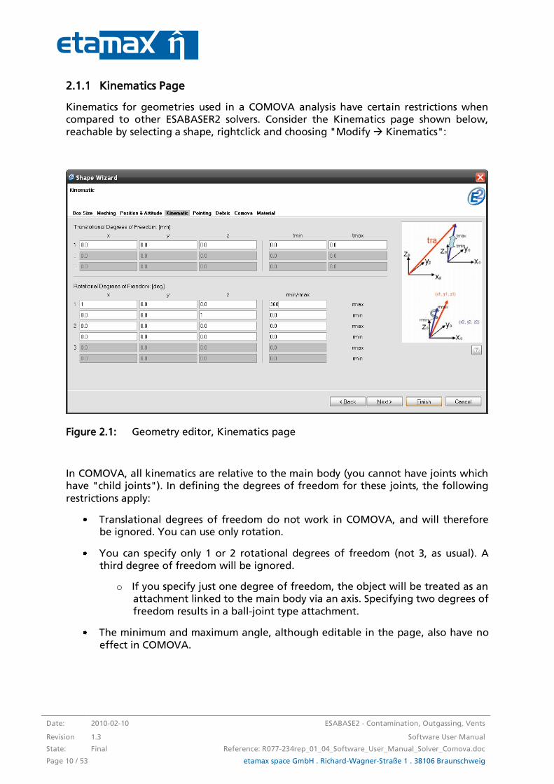
2.1.1 Kinematics Page

Kinematics for geometries used in a COMOVA analysis have certain restrictions when compared to other ESABASER2 solvers. Consider the Kinematics page shown below,

reachable by selecting a shape, rightclick and choosing "Modify Kinematics":

Figure 2.1: Geometry editor, Kinematics page

In COMOVA, all kinematics are relative to the main body (you cannot have joints which have "child joints"). In defining the degrees of freedom for these joints, the following

restrictions apply:

Translational degrees of freedom do not work in COMOVA, and will therefore be ignored. You can use only rotation.

You can specify only 1 or 2 rotational degrees of freedom (not 3, as usual). A third degree of freedom will be ignored.

o If you specify just one degree of freedom, the object will be treated as an attachment linked to the main body via an axis. Specifying two degrees of

freedom results in a ball-joint type attachment.

The minimum and maximum angle, although editable in the page, also have no

effect in COMOVA.





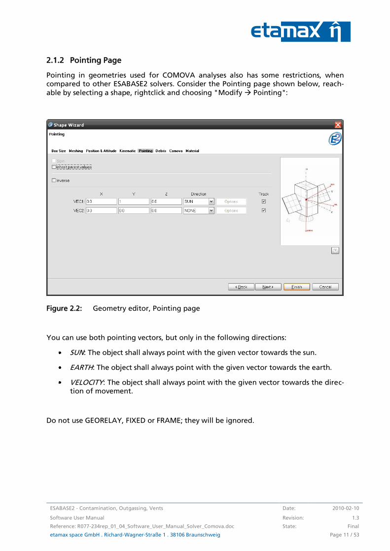
2.1.2 Pointing Page

Pointing in geometries used for COMOVA analyses also has some restrictions, when compared to other ESABASE2 solvers. Consider the Pointing page shown below, reach-

able by selecting a shape, rightclick and choosing "Modify Pointing":

Figure 2.2: Geometry editor, Pointing page

You can use both pointing vectors, but only in the following directions:

SUN: The object shall always point with the given vector towards the sun.

EARTH: The object shall always point with the given vector towards the earth.

VELOCITY: The object shall always point with the given vector towards the direc-tion of movement.

Do not use GEORELAY, FIXED or FRAME; they will be ignored.





2.1.3 COMOVA Page

COMOVA is quite rich in the information pertinent to the spacecraft geometry. In the geometry editor, select a shape by leftclicking it, open the context menu with a right-

click, and choose "Modify COMOVA". The wizard shown in the figure below appears.

Figure 2.3: Geometry editor, COMOVA page

The COMOVA page consists of several tabs, all working on the surfaces of a shape (e.g. one side of a cube), with the exception of the “chemical” tab.

Physics: The thickness of a surface.

Outgassing: What kind and how much matter is emitted (lost) on a given surface.

Chemical: Defines chemical properties used in outgassing.

Temperature: How hot or cold the surface is at different times.

Vents: How much matter is emitted from the surface at different times, e.g. for

thrusters.

Column densities: Defines view direction vectors for which column densities can be computed (a "column density" is the obstruction for optical instruments).





As a common element, each tab (except "Chemical") has two sections:

The upper section is for assigning a property to a surface, all surfaces, or perform a surface replacement.

The lower section is for actually defining that property.

The figure below shows a typical "property assignment" part (upper section of a tab).

Figure 2.4: Geometry editor, COMOVA page, Surface assignment

Assigning a property to a surface works in the same way as the material editor (see /1/). After you have defined a property (typically in the lower section), select one of the 3 radio buttons to work in three different styles:

All surfaces: Assign the property to all surfaces of the shape. This can be propa-gated to children (note: propagation is a "one-shot" action; the children need to

be already present to execute the propagation).

Individually: For each surface of the shape, make a dedicated assignment.

Replace: Replaces a previously selected property value with another value. This can be propagated to (already existing) children as well.

In the following, only the lower section of each tab will be discussed.





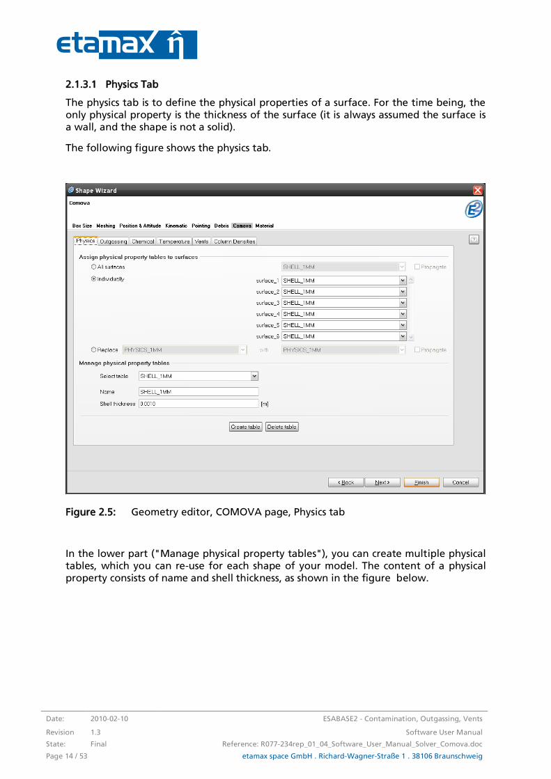
2.1.3.1 Physics Tab

The physics tab is to define the physical properties of a surface. For the time being, the only physical property is the thickness of the surface (it is always assumed the surface is a wall, and the shape is not a solid).

The following figure shows the physics tab.

Figure 2.5: Geometry editor, COMOVA page, Physics tab

In the lower part ("Manage physical property tables"), you can create multiple physical tables, which you can re-use for each shape of your model. The content of a physical property consists of name and shell thickness, as shown in the figure below.





Figure 2.6: Geometry editor, COMOVA page, Physics tab, table

Shell thickness is defined in m. Please note that this is different from most other places in ESABASE2, which usually work with mm.

The default physical table, which is selected at start for each surface, has a shell thick-ness of 1 millimeter. This has been done to be able to run a default analysis (which in-cludes computing of surfacic masses not yet outgassed).

Please note: Vents and physical property table assignments in combination have a side effect. When a surface is designed as a vent (see 2.1.3.5), all surfaces that share the same physical property table used by that surface will be treated as vents, too. You

should always create separated physical tables for vents.





2.1.3.2 Outgassing Tab

In the outgassing tab, you can define how much and which molecules are emitted by a surface, as shown in the screenshot below.

Figure 2.7: Geometry editor, COMOVA page, Outgassing tab

In the lower part ("Manage outgassing tables"), you can create multiple outgassing ta-bles, one of which can be assigned to each surface. Another option is to import out-gassing and chemical tables from an existing neutral file using the "Import tables…"

button.

By default, the file dialog will show the COMOVA plugin data folder, which contains the file outgassing_table.ntf. This neutral file contains a broad list of outgassing defini-

tions and chemical species.





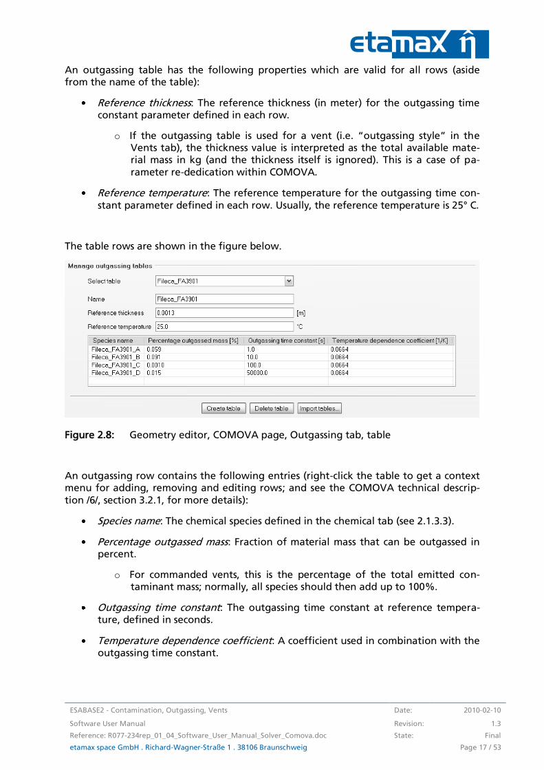
An outgassing table has the following properties which are valid for all rows (aside from the name of the table):

Reference thickness: The reference thickness (in meter) for the outgassing time constant parameter defined in each row.

o If the outgassing table is used for a vent (i.e. “outgassing style” in the Vents tab), the thickness value is interpreted as the total available mate-rial mass in kg (and the thickness itself is ignored). This is a case of pa-

rameter re-dedication within COMOVA.

Reference temperature: The reference temperature for the outgassing time con-

stant parameter defined in each row. Usually, the reference temperature is 25° C.

The table rows are shown in the figure below.

Figure 2.8: Geometry editor, COMOVA page, Outgassing tab, table

An outgassing row contains the following entries (right-click the table to get a context menu for adding, removing and editing rows; and see the COMOVA technical descrip-

tion /6/, section 3.2.1, for more details):

Species name: The chemical species defined in the chemical tab (see 2.1.3.3).

Percentage outgassed mass: Fraction of material mass that can be outgassed in percent.

o For commanded vents, this is the percentage of the total emitted con-taminant mass; normally, all species should then add up to 100%.

Outgassing time constant: The outgassing time constant at reference tempera-ture, defined in seconds.

Temperature dependence coefficient: A coefficient used in combination with the outgassing time constant.





In effect, each surface can have multiple chemical species, each with its own outgassing behaviour. It is also possible to have the same species twice, each time with different outgassing behaviour.





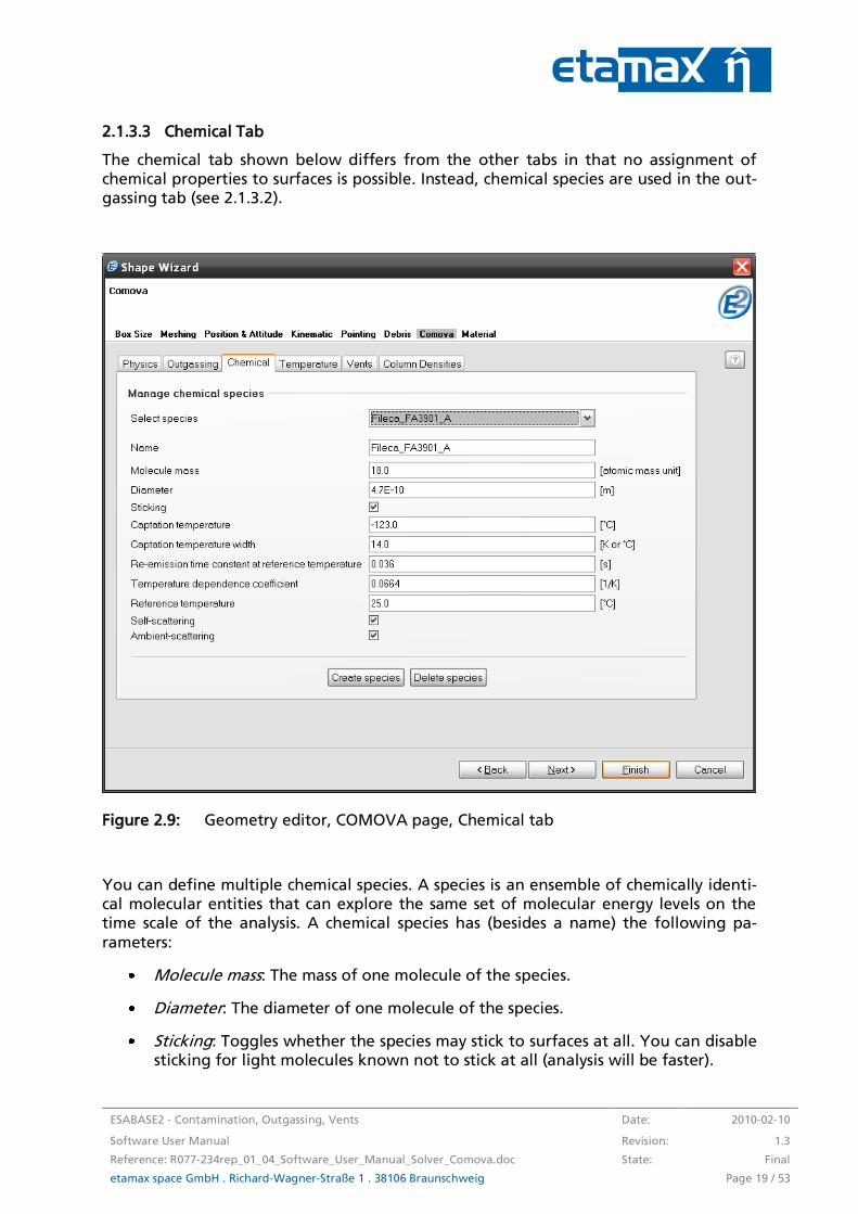
2.1.3.3 Chemical Tab

The chemical tab shown below differs from the other tabs in that no assignment of chemical properties to surfaces is possible. Instead, chemical species are used in the out-gassing tab (see 2.1.3.2).

Figure 2.9: Geometry editor, COMOVA page, Chemical tab

You can define multiple chemical species. A species is an ensemble of chemically identi-cal molecular entities that can explore the same set of molecular energy levels on the time scale of the analysis. A chemical species has (besides a name) the following pa-

rameters:

Molecule mass: The mass of one molecule of the species.

Diameter: The diameter of one molecule of the species.

Sticking: Toggles whether the species may stick to surfaces at all. You can disable sticking for light molecules known not to stick at all (analysis will be faster).





Captation temperature (Tc) and Captation temperature width (ΔTc): Define the temperature span (from Tc – ΔTc to Tc + ΔTc) in which bigger variations in sticking behaviour can occur.

o Above that range, sticking will become nearly impossible (everything will be reflected); below that range, sticking occurs almost always.

o The actual sticking coefficient is between 0 (no sticking) and 1 (all stick-ing) and is described fully in the COMOVA technical descriptions /6/, sec-

tion 3.3.1.

Re-emission variables: If you want neither sticking nor reflection, but instead the

re-emission of molecules after a certain delay, use the following options (more fully described in /6/, section 3.3.2).

o Re-emission time constant at reference temperature: How long it takes in seconds, before the molecule is re-emitted from the surface with a refer-ence temperature given here.

o Temperature dependence coefficient: Coefficient used together with the reference temperature.

o Reference temperature: The reference temperature used to describe the re-emission time constant above. Usually, the reference temperature is

25° C.

Self scattering: Toggles whether this chemical species’ molecules can collide with each other in the analysis.

Ambient scattering: Toggles whether this chemical species’ molecules can collide with the atmosphere molecules in the analysis.





2.1.3.4 Temperature Tab

In the temperature tab, you specify what temperature a surface is at during different times of the mission. The screenshot below shows the temperature tab.

Figure 2.10: Geometry editor, COMOVA page, Temperature tab

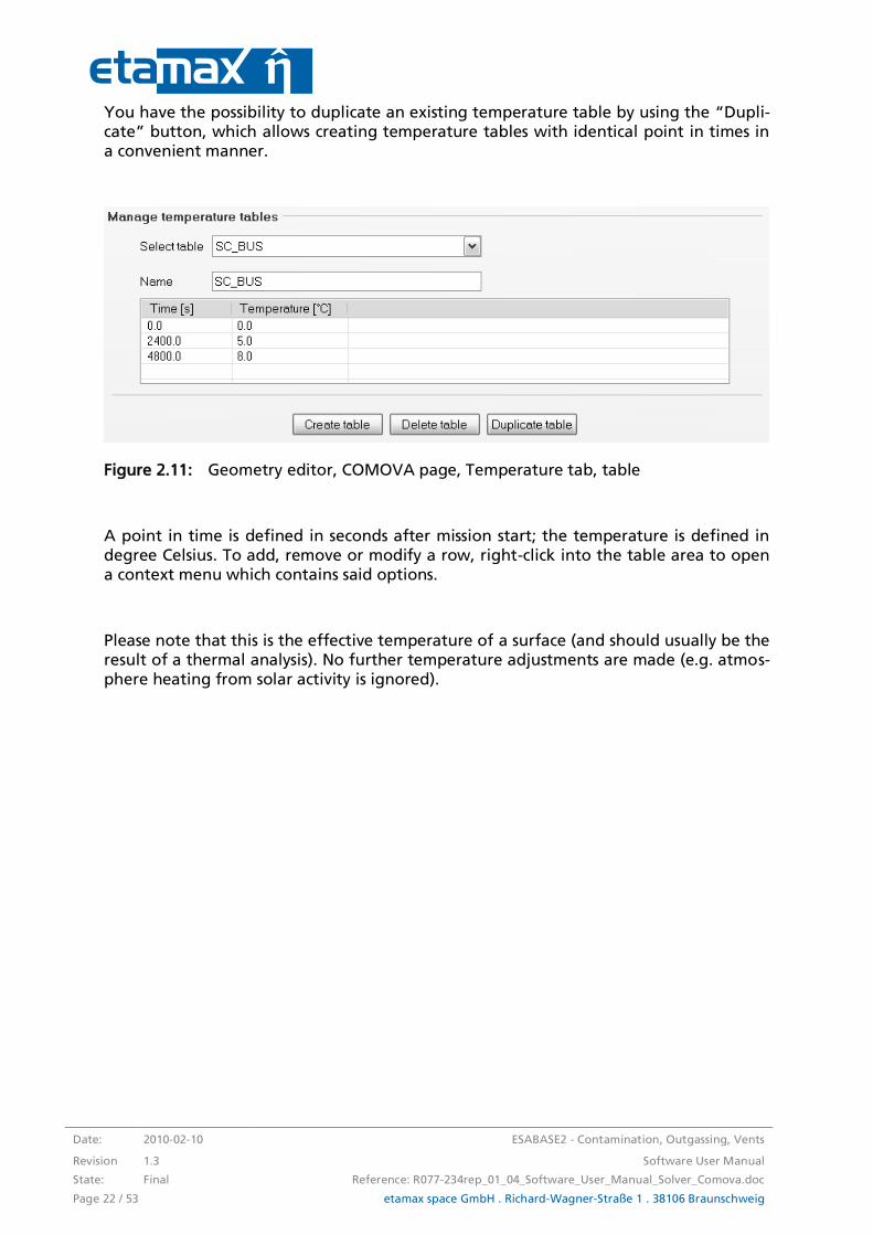
In the lower part ("Manage temperature tables"), you can specify multiple temperature tables, each consisting of a name and rows consisting of a point in time and a tempera-ture, as shown in the figure below.





You have the possibility to duplicate an existing temperature table by using the “Dupli-cate” button, which allows creating temperature tables with identical point in times in a convenient manner.

Figure 2.11: Geometry editor, COMOVA page, Temperature tab, table

A point in time is defined in seconds after mission start; the temperature is defined in degree Celsius. To add, remove or modify a row, right-click into the table area to open a context menu which contains said options.

Please note that this is the effective temperature of a surface (and should usually be the result of a thermal analysis). No further temperature adjustments are made (e.g. atmos-phere heating from solar activity is ignored).





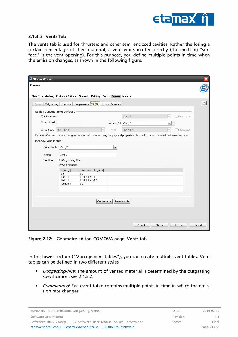
2.1.3.5 Vents Tab

The vents tab is used for thrusters and other semi enclosed cavities: Rather the losing a certain percentage of their material, a vent emits matter directly (the emitting "sur-face" is the vent opening). For this purpose, you define multiple points in time when

the emission changes, as shown in the following figure.

Figure 2.12: Geometry editor, COMOVA page, Vents tab

In the lower section ("Manage vent tables"), you can create multiple vent tables. Vent tables can be defined in two different styles:

Outgassing-like: The amount of vented material is determined by the outgassing specification, see 2.1.3.2.

Commanded: Each vent table contains multiple points in time in which the emis-sion rate changes.





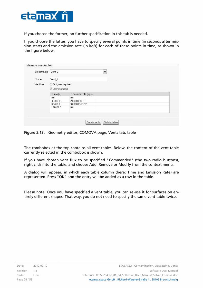
If you choose the former, no further specification in this tab is needed.

If you choose the latter, you have to specify several points in time (in seconds after mis-sion start) and the emission rate (in kg/s) for each of these points in time, as shown in the figure below.

Figure 2.13: Geometry editor, COMOVA page, Vents tab, table

The combobox at the top contains all vent tables. Below, the content of the vent table currently selected in the combobox is shown.

If you have chosen vent flux to be specified "Commanded" (the two radio buttons), right click into the table, and choose Add, Remove or Modify from the context menu.

A dialog will appear, in which each table column (here: Time and Emission Rate) are represented. Press "OK" and the entry will be added as a row in the table.

Please note: Once you have specified a vent table, you can re-use it for surfaces on en-tirely different shapes. That way, you do not need to specify the same vent table twice.





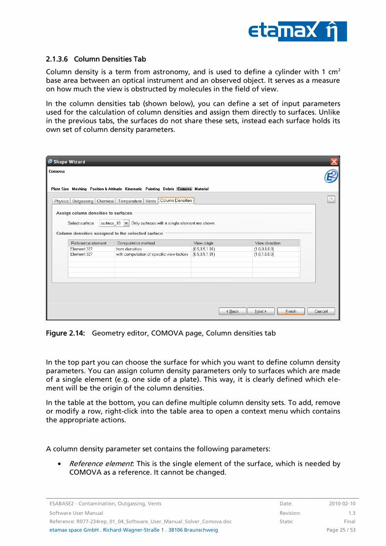
2.1.3.6 Column Densities Tab

Column density is a term from astronomy, and is used to define a cylinder with 1 cm2 base area between an optical instrument and an observed object. It serves as a measure on how much the view is obstructed by molecules in the field of view.

In the column densities tab (shown below), you can define a set of input parameters used for the calculation of column densities and assign them directly to surfaces. Unlike in the previous tabs, the surfaces do not share these sets, instead each surface holds its

own set of column density parameters.

Figure 2.14: Geometry editor, COMOVA page, Column densities tab

In the top part you can choose the surface for which you want to define column density parameters. You can assign column density parameters only to surfaces which are made of a single element (e.g. one side of a plate). This way, it is clearly defined which ele-

ment will be the origin of the column densities.

In the table at the bottom, you can define multiple column density sets. To add, remove or modify a row, right-click into the table area to open a context menu which contains

the appropriate actions.

A column density parameter set contains the following parameters:

Reference element: This is the single element of the surface, which is needed by COMOVA as a reference. It cannot be changed.





Computation method:

o From densities: Densities are computed in each volume element of the volume mesh and the column density is derived from that by integration along the viewing direction (in effect, "adding up" the volume cells that

obstruct the view).

o With computation of specific view factors: Densities are computed on sev-eral points on the viewing direction. The points are obtained from specific

computations based on special "view factors", which are ratios of local density to local outgassing fluxes on the spacecraft. The column density is

derived from that by integration along the viewing direction over values at those points.

View origin: A 3D coordinate which defines the origin of the view. By default, the center of the reference element is used.

View direction: A 3D coordinate which defines the direction of the view. Creates together with the view origin a line of sight pointing away from the reference element.

Please note:

Although the GUI supports the definition of column densities, later on (after the analysis) the column density results are only shown in the Listing file, and are not visualised in the 3D view of the result editor.

The computation method “From densities” only produces zero-value results. This is a known bug, however the cause of this error is currently unknown. Please use always “with computation of specific view factors” as the computation method

until the bug is fixed.





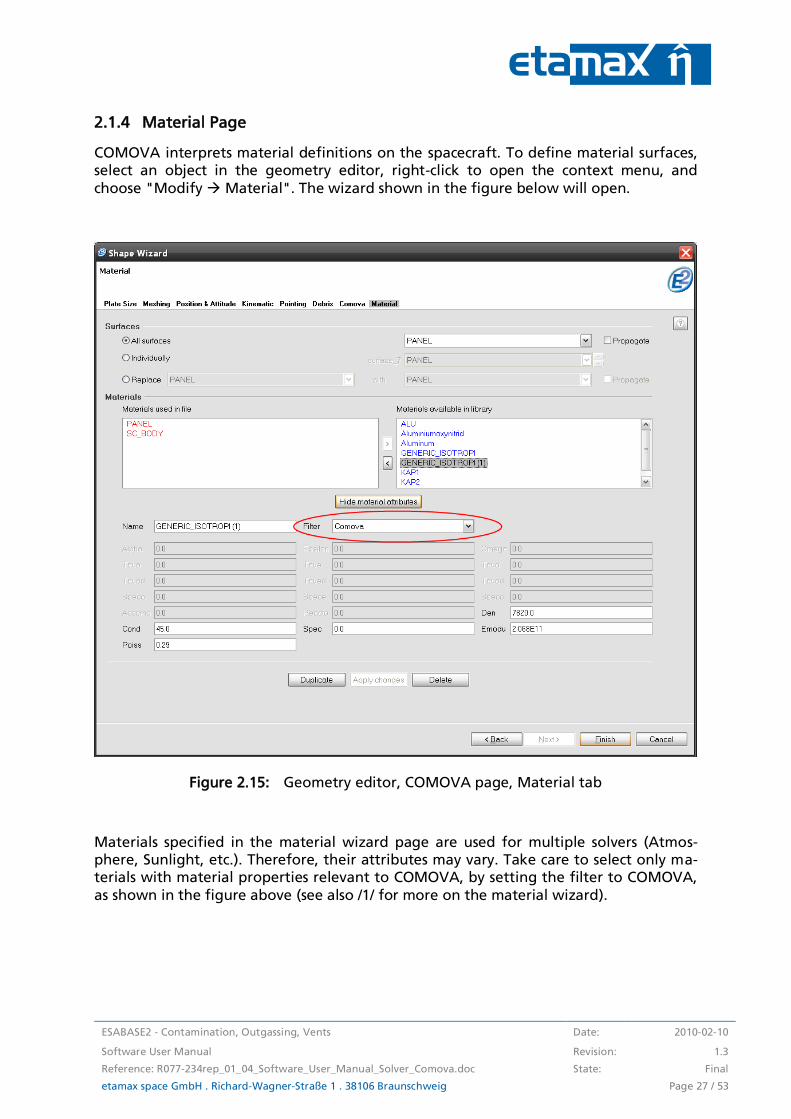
2.1.4 Material Page

COMOVA interprets material definitions on the spacecraft. To define material surfaces, select an object in the geometry editor, right-click to open the context menu, and

choose "Modify Material". The wizard shown in the figure below will open.

Figure 2.15: Geometry editor, COMOVA page, Material tab

Materials specified in the material wizard page are used for multiple solvers (Atmos-phere, Sunlight, etc.). Therefore, their attributes may vary. Take care to select only ma-terials with material properties relevant to COMOVA, by setting the filter to COMOVA,

as shown in the figure above (see also /1/ for more on the material wizard).





In particular, the COMOVA relevant material properties are:

Den: Density in [kg/m3].

Cond: Isotropic thermal conductivity in [J/m/K/s].

Spec: Specific heat at constant pressure in [J/kg/K].

Emodu: Isotropic Elasticity module in [N/m].

Poiss: Poisson number [dimensionless].





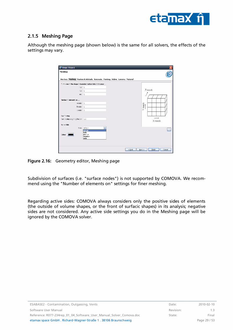
2.1.5 Meshing Page

Although the meshing page (shown below) is the same for all solvers, the effects of the settings may vary.

Figure 2.16: Geometry editor, Meshing page

Subdivision of surfaces (i.e. "surface nodes") is not supported by COMOVA. We recom-mend using the "Number of elements on" settings for finer meshing.

Regarding active sides: COMOVA always considers only the positive sides of elements (the outside of volume shapes, or the front of surfacic shapes) in its analysis; negative sides are not considered. Any active side settings you do in the Meshing page will be

ignored by the COMOVA solver.





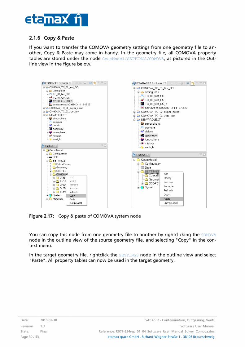
2.1.6 Copy & Paste

If you want to transfer the COMOVA geometry settings from one geometry file to an-other, Copy & Paste may come in handy. In the geometry file, all COMOVA property

tables are stored under the node GeomModel/SETTINGS/COMOVA, as pictured in the Out-

line view in the figure below.

Figure 2.17: Copy & paste of COMOVA system node

You can copy this node from one geometry file to another by rightclicking the COMOVA node in the outline view of the source geometry file, and selecting "Copy" in the con-

text menu.

In the target geometry file, rightclick the SETTINGS node in the outline view and select "Paste". All property tables can now be used in the target geometry.





2.2 COMOVA Input

Complementing the COMOVA information within the geometry, a global COMOVA in-put file specifies further analysis parameters. The figure below shows the COMOVA in-

put editor.

Figure 2.18: COMOVA input editor

The input editor has four different tabs (see bottom), concerned with different issues of a COMOVA analysis:

Physics: Reflection and scattering of molecules during the mission as well as den-sity and constituents of the atmospheric conditions the spacecraft goes through.

Raytracing and Numerics: Allows fine adjustment of raytracing detail (raytracing is the most time consuming activity in COMOVA).

Results: Which results to produce.

Ground Test Time Steps: Allows the input of time steps, which are needed for a COMOVA ground test run.

The following subsections describe the tabs.





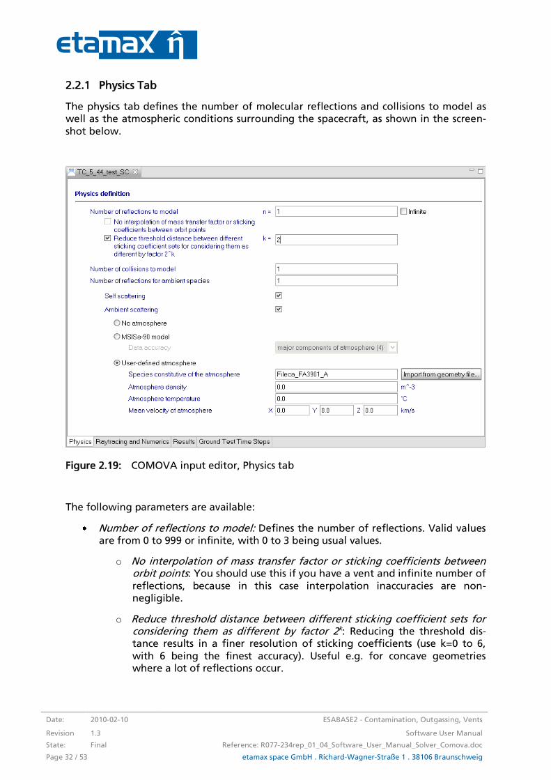
2.2.1 Physics Tab

The physics tab defines the number of molecular reflections and collisions to model as well as the atmospheric conditions surrounding the spacecraft, as shown in the screen-

shot below.

Figure 2.19: COMOVA input editor, Physics tab

The following parameters are available:

Number of reflections to model: Defines the number of reflections. Valid values are from 0 to 999 or infinite, with 0 to 3 being usual values.

o No interpolation of mass transfer factor or sticking coefficients between orbit points: You should use this if you have a vent and infinite number of

reflections, because in this case interpolation inaccuracies are non-negligible.

o Reduce threshold distance between different sticking coefficient sets for considering them as different by factor 2k: Reducing the threshold dis-tance results in a finer resolution of sticking coefficients (use k=0 to 6,

with 6 being the finest accuracy). Useful e.g. for concave geometries where a lot of reflections occur.





Number of collisions to model: Defines the number of collisions between chemi-cal species. Usually 0, set to1 for low, and 2 for very low earth orbits.

Number of reflections for ambient species: Defines the number of reflections for ambient species (i.e. the atmosphere around the spacecraft). These bouncing

molecules can hit the ram face of the spacecraft, thus increasing atmospheric

drag.

Self scattering: Toggles, whether self scattering (collision of outgassed molecules with themselves) should be integrated into the calculation. Self scattering can be

enabled if the number of collisions to model was set to a value bigger than zero.

Ambient scattering: Toggles whether ambient scattering (collision of outgassed molecules with the atmosphere) should be integrated into the calculation. Am-

bient scattering can be enabled if the number of collisions to model and the number of reflections for ambient species were set to a value bigger than zero.

Mass transfer factors (including reflections) are only computed for a few reference stick-ing coefficient sets. During the computation, for an arbitrary sticking coefficient set, the mass transfer factor obtained from the nearest reference sticking coefficient set is used,

which involves a small error. This error can be reduced by reducing the threshold dis-tance that triggers the computation of another reference sticking coefficient set.

If ambient scattering is enabled, you can define the atmosphere which surrounds the spacecraft by choosing one of the three following options:

No atmosphere

MSISe-90 model

User-defined atmosphere

Having no atmosphere has no further options.

When choosing an MSISe-90 model, you can define the accuracy of the atmospheric modelling:

Only major atmosphere component (1): Use only the major atmosphere compo-nent (i.e. the most common molecule type; usually atomic oxygen for LEO) for the considered orbit. Fastest option.

Only atomic oxygen (2): Use only atomic oxygen.

Only equivalent species (3): Use one equivalent species (“average” of all available species), as close as possible to the total atmosphere effect.





Major components of atmosphere (4): Use the major components of the atmos-phere (the densest species plus all species that have at least 10% of the densest one).

All 7 species given by MSISe-90 (5): Use all seven species given by MSISe-90, which are: atomic oxygen, molecular oxygen, atomic nitrogen, molecular nitrogen,

atomic hydrogen, helium and argon. Slowest option.

When defining your own atmosphere, first import the species constitutive of the at-mosphere from a geometry file (coming from your spacecraft definition). This ensures

that the same chemical species used in the geometry file are used here.

Additionally, define the three parameters below:

Atmosphere density in 1/m3: Density of the atmosphere in particles per m³.

Atmosphere temperature in °C: The constant temperature of the atmosphere. Variations are not taken into account. Useful also for ground tests (which need a

defined constant background temperature).

Mean velocity of atmosphere in km/s in x/y/z direction: Defines the velocity of the atmosphere, i.e. the wind speed in the spacecraft reference frame.

Please note: When you choose MSIS as atmosphere model, and ambient scattering is enabled, there are some transport parameter combinations that result in an analysis error. This is a known but uninvestigated bug. Please avoid the following and similar

transport settings:

Parameter Set 1 Parameter Set 2

Number of reflections to model !=0 0

Number of collisions to model !=0 1

Number of reflections for ambient species not important 1

Ambient scattering Enabled Enabled

Self scattering not important Enabled

Atmosphere MSIS MSIS

Future versions of COMOVA will address this bug.





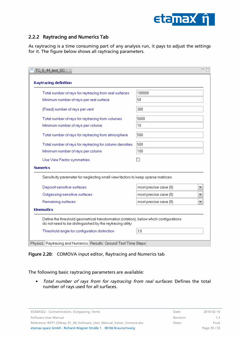
2.2.2 Raytracing and Numerics Tab

As raytracing is a time consuming part of any analysis run, it pays to adjust the settings for it. The figure below shows all raytracing parameters.

Figure 2.20: COMOVA input editor, Raytracing and Numerics tab

The following basic raytracing parameters are available:

Total number of rays from for raytracing from real surfaces: Defines the total number of rays used for all surfaces.





Minimum number of rays per real surface: Defines the minimum number of rays used for each surface.

o During raytracing, first the total number of rays is distributed to the sur-faces according to their respective surface areas. Then, any surface not

getting the minimum number of rays is supplemented with additional rays.

Fixed number of rays per vent: Defines the number of rays used for each vent.

Total number of rays for raytracing from volumes: Defines the total amount of rays used for the volume cells surrounding the spacecraft (for backscattering of

emitted molecules to spacecraft).

Minimum number of rays per volume: Defines the minimum amount of rays used for each volume cell sourrounding the spacecraft.

Total number of rays for raytracing from atmosphere: Defines the total amount of rays used for the effect of atmospheric particles.

Total number of rays for raytracing for column densities: Defines the total amount of rays used for the column densities.

o A column density is a cylinder (usually of 1 cm2 base area) from an optical instrument to a far object. The number of molecules in it determines how much the view is obstructed.

Mininum number of rays per column: Defines the minimum amount of rays used for each column density. Total/minimum number of rays works the same way as for real surfaces, see above.

Use View Factor symmetries: Toggles the usage of view factor symmetries in the raytracing process. This is good for fluxes on small surfaces, is usually enabled, and more fully described in /6/.

In the "Numerics" section, further parameters can limit the computational effort. For each category of surfaces, you can decide to ignore small view factors. The view factor is the percentage of flux emitted by one surface that reaches another surface. When a

view factor is very small, it might as well be ignored.

The surface categories (for which you can finetune the settings) are:

Deposit-sensitive surfaces: Surfaces which are sensitive to deposits.

Outgassing-sensitive surfaces: Surfaces which are sensitive to outgassing.

Remaining surfaces: All other surfaces that do not fall under the previous two categories.

The possible sensitivity values are:





Most precise case: Use all view factors.

Only very small VF neglected: Skip very small view factors during the computa-tion.

Only small VF neglected: Skip small view factors during computation.

Only large VF retained: Use only large view factors during the computation.

Only very large VF are retained: Use only very large view factors during the com-putation.

Finally, in the "Kinematics" section, you can define one parameter:

Threshold angle for configuration distinction: Defines the threshold geometrical transformation (rotation) below which kinematic configurations do not need to

be distinguished by the raytracing utility. This is expressed as the maximum rota-tion angle over all attachments of the spacecraft.





2.2.3 Results Tab

The results tab is for specifying which results you want from a COMOVA run. The avail-able parameters are shown in the figure below.

Figure 2.21: COMOVA input editor, Result tab





In the "Computed data" section, you can specify which physical quantities are to be provided as output:

Surfacic masses of contaminant not yet outgassed: The masses of contaminant material not yet outgassed. Short: CNTSMS [kg/m2].

Masses of deposited contaminant: The masses of deposited contaminant (~ "im-pinging minus reflected/re-emitted") per element. Short: DEPMSS [kg/element].

Instantaneous outgassed flux: The outgassed flux. Short: OUTFLX [kg/m²/s].

Instantaneous re-emitted flux: The re-emitted flux. Short: REMFLX [kg/m²/s].

Instantaneous impinging flux: The impinging flux (~ "deposited plus reflected/re-emitted"). Short: IMPFLX [kg/m²/s].

Instantaneous deposited flux: The deposited flux (~ "impinging minus re-flected/re-emitted"). Short: DEPSMS [kg/m²].

Volume density: The volume density for each volume cell around the spacecraft.

o Please note: These results will only be visible in the listing file, not graphi-cally in the 3D model of the spacecraft. Short: CNTDEN [m-3]

Column density: The column density results for each column density defined in the geometry.

o Please note: These results will only be visible in the listing file, not graphi-cally in the 3D model of the spacecraft. Short: CD_TOTAL [m-2] and CD_OBSCUR [-]

Only total contaminant masses and fluxes are given: Toggles whether the results above will be shown separately for each involved chemical species or just the to-tal results, which is the summation of all species.

In the "Time steps" section, you can specify either explicit time steps or combine addi-tive selection criteria.

If you prefer explicit time steps, you have to define a series of time steps separated by comma (e.g. "10.0, 1000.0, 1350.5"). The time steps are defined in seconds after mission start. The time steps should be multiples of the "time interval between orbital points",

defined in the ESABASE2 mission editor (see core user manual /1/).

If you prefer a criteria-based selection of orbital points, the time steps are chosen dy-namically according to the following criteria:

At user-defined orbital points: For every n-th orbital point, generate results, e.g. if this is set to 1, results will be generated for every orbital point. If it set to 3, results will be generated for every third orbital point.

At times for which temperature is given: Generate results for each time step for which a temperature was defined (see 2.1.3.4).





At an user-defined number of points per orbit: Divides the orbit into n points and generates a result for each point.

Every delta t, a user-defined time step: Every specified time step, a result will be generated.

In the original COMOVA, further options were available, if multiple orbits were de-fined. They have been deactivated in ESABASE2 because the mission editor only defines

one orbit.

At interpolated orbital points.

Every user-defined orbits.

For interpolated orbits.





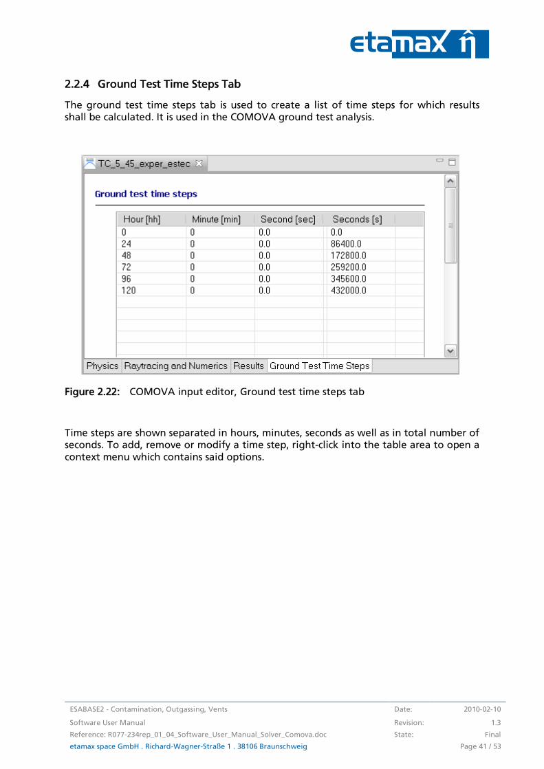
2.2.4 Ground Test Time Steps Tab

The ground test time steps tab is used to create a list of time steps for which results shall be calculated. It is used in the COMOVA ground test analysis.

Figure 2.22: COMOVA input editor, Ground test time steps tab

Time steps are shown separated in hours, minutes, seconds as well as in total number of seconds. To add, remove or modify a time step, right-click into the table area to open a context menu which contains said options.





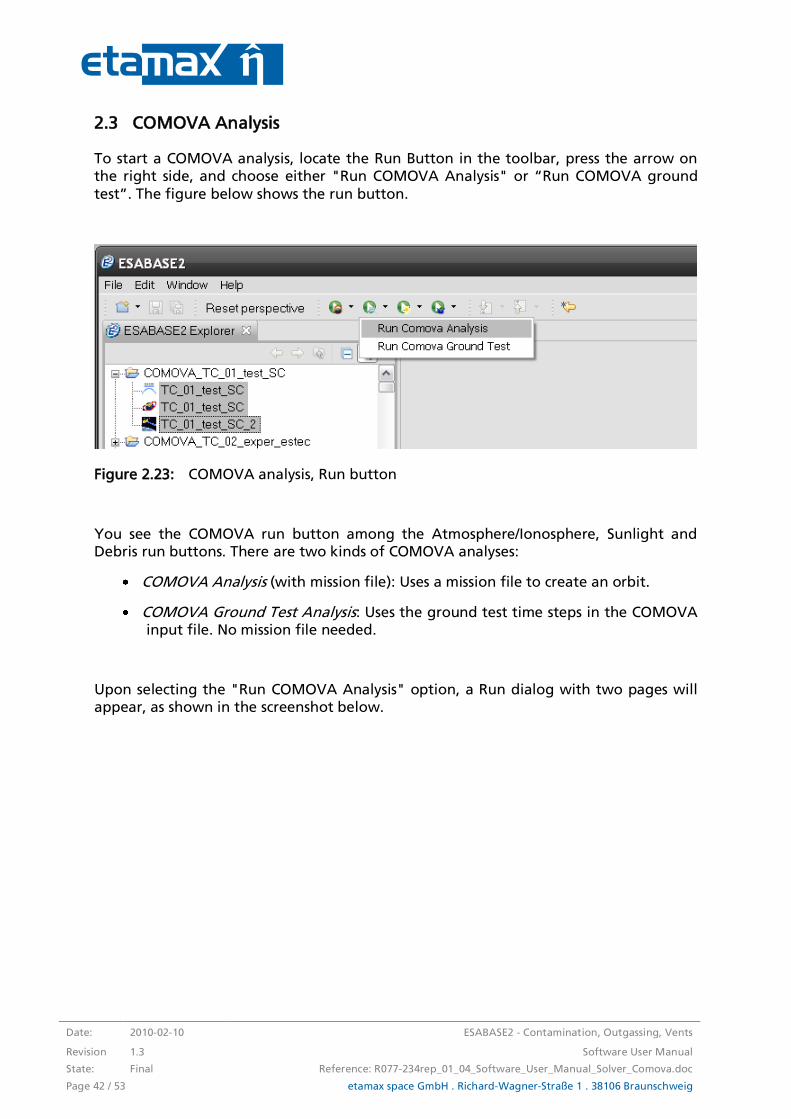
2.3 COMOVA Analysis

To start a COMOVA analysis, locate the Run Button in the toolbar, press the arrow on the right side, and choose either "Run COMOVA Analysis" or “Run COMOVA ground

test”. The figure below shows the run button.

Figure 2.23: COMOVA analysis, Run button

You see the COMOVA run button among the Atmosphere/Ionosphere, Sunlight and Debris run buttons. There are two kinds of COMOVA analyses:

COMOVA Analysis (with mission file): Uses a mission file to create an orbit.

COMOVA Ground Test Analysis: Uses the ground test time steps in the COMOVA input file. No mission file needed.

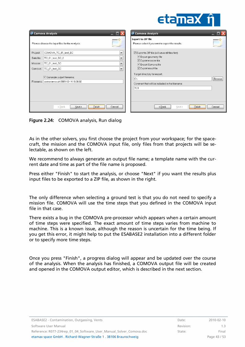
Upon selecting the "Run COMOVA Analysis" option, a Run dialog with two pages will appear, as shown in the screenshot below.





Figure 2.24: COMOVA analysis, Run dialog

As in the other solvers, you first choose the project from your workspace; for the space-craft, the mission and the COMOVA input file, only files from that projects will be se-

lectable, as shown on the left.

We recommend to always generate an output file name; a template name with the cur-rent date and time as part of the file name is proposed.

Press either "Finish" to start the analysis, or choose "Next" if you want the results plus input files to be exported to a ZIP file, as shown in the right.

The only difference when selecting a ground test is that you do not need to specify a mission file. COMOVA will use the time steps that you defined in the COMOVA input

file in that case.

There exists a bug in the COMOVA pre-processor which appears when a certain amount of time steps were specified. The exact amount of time steps varies from machine to

machine. This is a known issue, although the reason is uncertain for the time being. If you get this error, it might help to put the ESABASE2 installation into a different folder

or to specify more time steps.

Once you press "Finish", a progress dialog will appear and be updated over the course of the analysis. When the analysis has finished, a COMOVA output file will be created

and opened in the COMOVA output editor, which is described in the next section.





2.4 COMOVA Results

A geometric COMOVA analysis produces a COMOVA result file, which is interpreted by the COMOVA result editor. The editor contains the following functionalities:

3D Results: Shows the spacecraft geometry overlaid with the contamination or other output parameters.

Listings: Shows the NTF ("neutral file format") output of the COMOVA solver ex-ecutable. This is the raw input used for the creation of the result file.

Notes: A blank text area for your own notes.

2.4.1 3D Results

The following figure shows the "3D Results" tab in a COMOVA result editor.

Figure 2.25: COMOVA result editor, 3D Results

You can see a spacecraft geometry with element numbers, visualised by colour codes on the elements and decoded by the colour scale on the right. At the top of the editor, the same toolbar as in the geometry editor appears, allowing you to zoom, rotate and scroll

around the spacecraft.





Additionally, you can rightclick into the 3D area to invoke the context menu, which contains the following options:

Colour: Defines the result value to be laid over the S/C geometry; default is ele-ment number.

Time step: Which time step to show (note: there are no combined "mission" re-sults in COMOVA).

Coordinate Systems: Whether to display coordinate systems alongside the S/C geometry.

Element Chart: Shows the results for one single geometrical element (select one with Shift+Leftclick to enable).

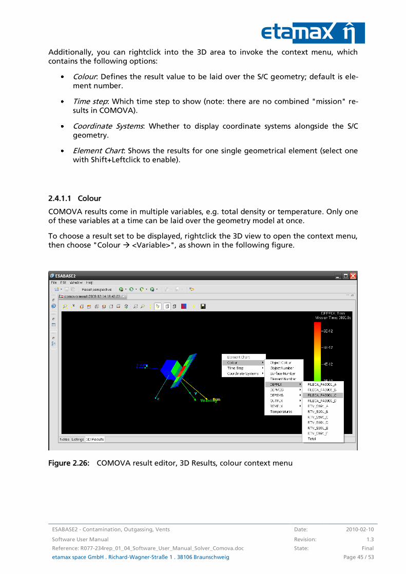
2.4.1.1 Colour

COMOVA results come in multiple variables, e.g. total density or temperature. Only one of these variables at a time can be laid over the geometry model at once.

To choose a result set to be displayed, rightclick the 3D view to open the context menu, then choose "Colour <Variable>", as shown in the following figure.

Figure 2.26: COMOVA result editor, 3D Results, colour context menu





The first 4 items in the context menu are not part of the COMOVA results; instead they are used to gain an overview of the spacecraft geometry, and particular its objects, sur-faces and elements.

Object Colour: Displays exactly the same object colour which was used in the ge-ometry editor.

Object Number: Each object is identified by an object number. In this overlay,

this object number is mapped to colours.

o Leftclick on an object in the 3D view to select it, and then look at the col-our scale to the right. The appropriate colour will be marked, and the ob-

ject number will be shown.

Surface Number: Breaking down the objects, each surface is shown in a different colour.

o Ctrl+leftclick on a surface in the 3D view to select it. The respective surface number is marked in the colour scale to the right.

Element Number: Further breaking down the surfaces, each element is shown in a different colour.

o Shift+leftclick on an element in the 3D view. The selected element num-ber and color will be marked in the color scale.

The following 9 items show the respective quantity (listed below) as colours on the ele-ments of the geometry model. To see the exact value on an element, Shift+leftclick the

element; the colour scale on the right will then show the quantity value.

CNTSMS [kg/m²]: The surfacic masses of contaminant not yet outgassed (i.e. re-

maining in the emitting material).

DEPFLX [kg/m²/s]: The instantaneous deposited flux per second.

DEPMSS [kg/element]: The total mass of deposited contaminant on surfaces (counted per element, not per square meter).

DEPSMS [kg/m²]: The surfacic mass of deposited contaminant, per square meter.

IMPFLX [kg/m²/s]: The instantaneous impinging flux. "Impinging" includes both

deposited and reflected/re-emitted particles.

OUTFLX [kg/m²/s]: The instantaneous outgassed flux (constantly subtracting from

CNTSMS).

REMFLX [kg/m²/s]: The instantaneous re-emitted flux (i.e. the impinging flux

which is deposited and then re-emitted (as opposed to simply being reflected)).

Temperature [°C]: The temperature of the element.

Emissions from vents and outgassing have different units. A vent is considered as a sin-gularity (i.e. “has no surface”) and has an emission in [kg/s], while outgassing flux is from a surface and is in [kg/m2/s]. However, in order to be able to display emissions





from vents and from outgassing on the same plot, the units of these emissions are both

displayed in the same colour scale and unit, [kg/m2/s] for OUTFLX.

This display is simply wrong for vents, and the displayed number is to be understood as in units of [kg/s]. In case of the remaining mass CNTSMS, the same is true: whereas dis-

played in [kg/m2] on the colour scale as for the remaining contaminant mass, the re-maining vent mass (relevant for continuously open vents only) is to be understood as in

units of [kg].

Please note: The number of options that is actually visible depend on your choices in the Result tab of the COMOVA input editor (see 2.2.3). Only temperature will always be

visible.





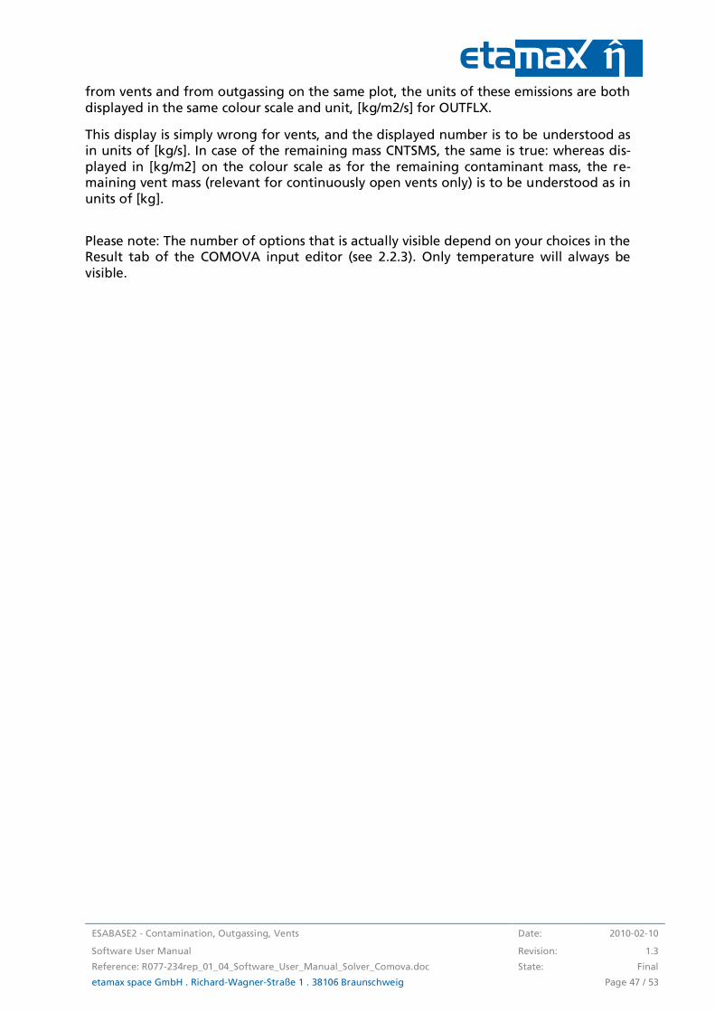
2.4.1.2 Time step

When the COMOVA result editor opens, it shows the analysis results for the first time step (no "mission" results in COMOVA). You can view the other time steps by opening the context menu and navigating to "Time Step", as shown in the following figure.

Figure 2.27: COMOVA result editor, 3D Results, Orbital Point context menu

In addition to the coordinate system, Earth, Sun and velocity direction are shown as de-picted above (earth in blue, sun in yellow, velocity in green).

These vectors do not exist for a ground test result and can therefore not be visualized in that case.





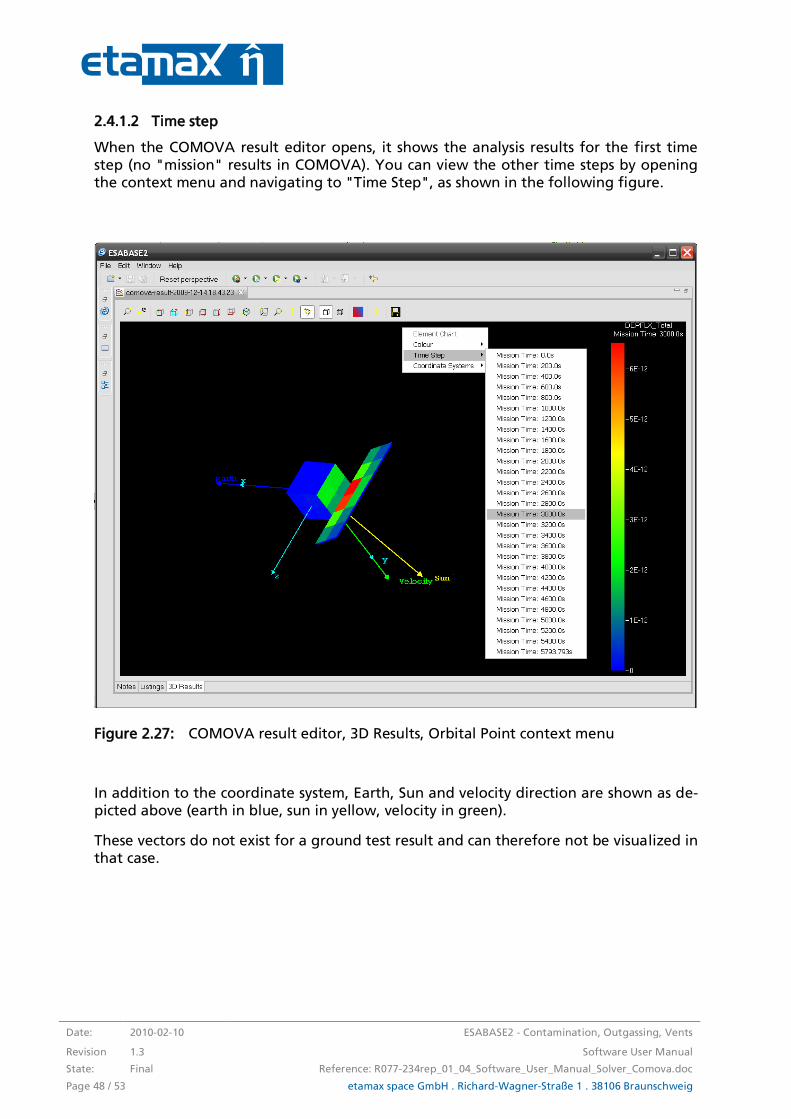
2.4.1.3 Coordinate Systems

To visualise the coordinate system you used previously in the geometry editor, change the coordinate system by opening the context menu and navigating to "Coordinate Systems", as shown in the following figure.

Figure 2.28: COMOVA result editor, 3D Results, Coordinate Systems context menu

You can choose among the following coordinate system settings:

No coordinates: Note that pointing vectors will also be deactivated.

Global coordinate system (centred): Shows the xyz-axis for the entire system.

Global coordinate system in the corner: Same as before, but in the corner of the system, not centred.

Global and local coordinate systems: Shows xyz-axis for each object. Detailed but probably slightly irritating for complex S/C geometries.





2.4.1.4 Element Chart

Apart from results for the entire spacecraft, you can also view dedicated results for sin-gle elements of the geometry, in the form of 2D graphs called "Element Chart".

Shift+Leftclick an element of the S/C geometry, then open the context menu and select "Element Chart". The following figure shows the resulting small popup window.

Figure 2.29: COMOVA result editor, 3D Results, Element Chart

From the "Result Set" combo-box, select a variable; the appropriate graph for the given element will be displayed, as shown on the right. These are the same values that are colour coded in the element in the 3D view.

You also have the possibility to adjust the appearance of the graph via the “Options” button, and to export the image as PNG or JPG via the “Export Image” button.





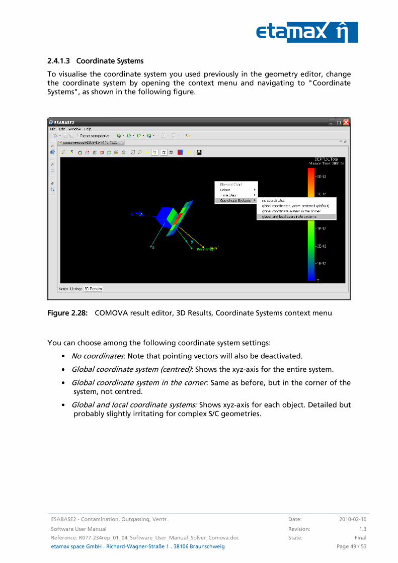
2.4.2 Listings

When you run a COMOVA analysis, ESABASE2 internally uses a COMOVA solver execu-table which yields output text files, which are then converted into a COMOVA result

file. In the Listings tab, you can view these raw text outputs directly, as shown in the figure below.

Figure 2.30: COMOVA result editor, Listings

The tab is made of a combobox for selecting the file to view, and a text area which shows the selected file. The following files are available:

COMOVA output file

COMOVA runtime log

Intermediate file





Detailed information about the contents of the listing files can be found in the original COMOVA user manual /5/.

Please note: The listing files are foremost saved as data nodes in the COMOVA result file. Additionally, they are written in ASCII format to the "Listings" subfolder of the cur-

rent project folder, in order to be more easily accessible to post-processing tools.

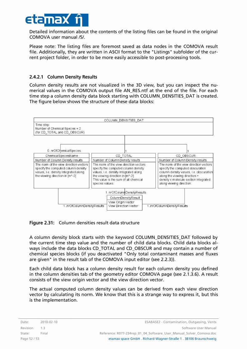
2.4.2.1 Column Density Results

Column density results are not visualized in the 3D view, but you can inspect the nu-merical values in the COMOVA output file AN_RES.ntf at the end of the file. For each time step a column density data block starting with COLUMN_DENSITIES_DAT is created.

The figure below shows the structure of these data blocks:

Figure 2.31: Column densities result data structure

A column density block starts with the keyword COLUMN_DENSITIES_DAT followed by the current time step value and the number of child data blocks. Child data blocks al-

ways include the data blocks CD_TOTAL and CD_OBSCUR and may contain a number of chemical species blocks (if you deactivated "Only total contaminant masses and fluxes

are given" in the result tab of the COMOVA input editor (see 2.2.3)).

Each child data block has a column density result for each column density you defined in the column densities tab of the geometry editor COMOVA page (see 2.1.3.6). A result

consists of the view origin vector and the view direction vector.

The actual computed column density values can be derived from each view direction vector by calculating its norm. We know that this is a strange way to express it, but this

is the implementation.





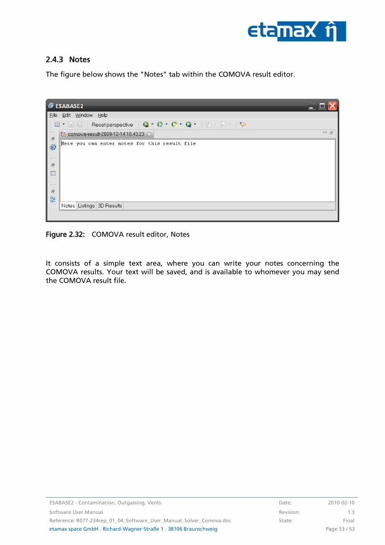
2.4.3 Notes

The figure below shows the "Notes" tab within the COMOVA result editor.

Figure 2.32: COMOVA result editor, Notes

It consists of a simple text area, where you can write your notes concerning the COMOVA results. Your text will be saved, and is available to whomever you may send

the COMOVA result file.

Documents

ESABASE2 - Contamination, Outgassing, Ventsesabase2.net/.../uploads/2015/12/ESABASE2-Comova-User-Manual.pdf · ESABASE2 - Contamination, Outgassing, Vents Date: 2010-02-10 Software