Embed Size (px)
Citation preview
© etamax space GmbH
ESABASE2 - Debris
Software User Manual
Contract No: 16852/02/NL/JA
Title: PC Version of DEBRIS Impact Analysis Tool
ESA Technical Officer: G. Drolshagen, J. Sørensen
Prime Contractor: etamax space GmbH
Authors: K. Ruhl, K.D. Bunte, A. Gaede, A. Miller
Date: 2014-11-20
Reference: R077-232rep_01_07_01_Software_User_Manual_Solver_Debris.doc
Revision: 1.7.1
Status: Final
Confidentiality: Public
etamax space GmbH
Frankfurter Str. 3 d
D-38122 Braunschweig
Germany
Tel.: +49 (0)531.866688.30
Fax: +49 (0)531.866688.99
email: [email protected]
http://www.etamax.de
Date: 2014-11-20 ESABASE2 - Debris
Revision 1.7.1 Software User Manual
State: Final Reference: R077-232rep_01_07_01_Software_User_Manual_Solver_Debris.doc
Page 2 / 78 etamax space GmbH . Frankfurter Str. 3 d . 38122 Braunschweig
Table of Contents
2.1 Debris Geometry ...................................................................................... 11
2.1.1 Debris Page ................................................................................................. 12
2.1.2 Meshing Page .............................................................................................. 14
2.2 Debris Input ............................................................................................ 15
2.2.1 Debris Main Tab ........................................................................................... 15
2.2.2 Debris Ground Test Tab ................................................................................ 41
2.2.3 Debris Non-Geometric Analysis Tab ............................................................... 43
2.3 Debris Analysis ........................................................................................ 45
2.3.1 Geometric Debris Analysis ............................................................................. 46
2.3.2 Non-geometric Debris Analysis ...................................................................... 50
2.4 Debris Results ......................................................................................... 52
2.4.1 3D Results ................................................................................................... 52
2.4.2 2D Results ................................................................................................... 58
2.4.3 Listings ....................................................................................................... 63
2.4.4 Notes .......................................................................................................... 65
3.1 Lunar Mission .......................................................................................... 66
3.1.1 Abstraction of the Lunar Mission .................................................................... 67
3.1.2 Trajectory File ............................................................................................. 70
3.1.3 Specifics for Abstracted Lunar Mission............................................................ 72
3.1.4 Specifics for Trajectory File ........................................................................... 74
3.2 Perform an Analysis ................................................................................. 74
4.1 Specific Information for Analyses on L1/L2 Orbits ...................................... 76
4.1.1 L1/L2 Orbits with Mission File ........................................................................ 76
4.1.2 L1/L2 Orbit Definition via Trajectory file ......................................................... 78

ESABASE2 - Debris Date: 2014-11-20
Software User Manual Revision: 1.7.1
Reference: R077-232rep_01_07_01_Software_User_Manual_Solver_Debris.doc State: Final
etamax space GmbH . Frankfurter Str. 3 d . 38122 Braunschweig Page 3 / 78
Document Information
I. Release Note
Name Function Date Signature
Established by: K. Ruhl, K.D. Bunte, A.
Gaede, A. Miller
Technical Project Manager
2014-11-20
Released by: K.D. Bunte Project Manager 2014-11-20
II. Revision History
Version Date Initials Changed Reason for Revision
0.1 2009-08-03 KR All Split from common ESABASE2 handbook.
0.2 2009-09-22 KR Debris Solver Improved model selection description.
0.9 2009-09-25 KB All Review for Final draft
1.0 2009-09-28 KR All Update after review
1.1 2009-12-14 KR Section 2.1 Pos/negative side results.
1.2 2010-08-23 KB Section 2.2.1.5, all
Description of the use of the User Subroutine ex-tended; document layout update
1.4 2012-12-04 AG Section 2.2 Modified BLE and Shielding handling
1.5 2013-04-19 AM Sections 2.2.1.1, 2.4.2, 3
Extended for Lunar missions consideration.
1.5.1 2013-07-09 AM Sections 2.2.1.1.1, 2.2.1.1.2, 2.2.1.1.3
Clarification of the used date for MASTER popula-tion snapshots.
1.5.2 2013-11-07 AM Section 2.4.3.1 Introduction of Crater vs. Crater size listing inter-pretation.
1.6 2014-03-19 AM Sections 2.2.1.5, 3.1.2, 4
Extended for L1/L2 orbits consideration, change to Intel Fortran Compiler.
1.7 2014-07-24 AM Sections 2.2.1.1, 2.4.2, 3.1.3.1, 3.1.4, 4.1.2
Extended for ORDEM 3.0 model use.
1.7.1 2014-11-20 AM Sections 2.2.1.1 Introduction of notes for ORDEM 3.0 use

Date: 2014-11-20 ESABASE2 - Debris
Revision 1.7.1 Software User Manual
State: Final Reference: R077-232rep_01_07_01_Software_User_Manual_Solver_Debris.doc
Page 4 / 78 etamax space GmbH . Frankfurter Str. 3 d . 38122 Braunschweig
III. Distribution List
Institution Name Remarks
ESTEC Gerhard Drolshagen
etamax space ESABASE2 team
various ESABASE2 licenssees
IV. List of References
/1/ K. Ruhl, K.D. Bunte, ESABASE2/Framework software user manual, R077-230rep, ESA/ESTEC Contract 16852/02/NL/JA "PC Version of DEBRIS Impact Analysis Tool", etamax space, 2009
/2/ A. Gäde, K.D. Bunte, ESABASE2/Debris Technical Description, ESA/ESTEC Contract 16852/02/NL/JA "PC Version of DEBRIS Impact Analysis Tool", etamax space, July 2009
/3/ ESABASE2 homepage, http://www.esabase2.net/
/4/ ESABASE User Manual, ESABASE/GEN-UM-070, Issue 1, Mathematics & Software Di-vision, ESTEC, March 1994
/5/ Giunta, I.; Lemcke, C.; Roussel, J.F.; COMOVA 1.1, Technical Description, ESTEC
Contract No. 12867/98/NL/PA, HTS AG and ONERA, March, 2002
/6/ Giunta, I.; Lemcke, C.; Roussel, J.F.; COMOVA 1.1.10, Software User Manual, ESTEC
Contract No. 12867/98/NL/PA, HTS AG and ONERA, October, 2006
/7/ Borde, J., Sabbathier, G. de, Development of an Improved Atomic Oxygen Analysis
Tool, Software User Manual, S413/NT/19.94, Issue 2, ESTEC Contract
9558/91/NL/JG, Matra Marconi Space, Toulouse, France, May 1994
/8/ ESABASE/Sunlight Application Manual, ESABASE/SUN-UM-072, Issue 2, Rel. 2.1,
ESTEC, Mathematics & Software Division, Noordwijk, The Netherlands, September
1994
/9/ Bendisch, J., K.D. Bunte, S. Hauptmann, H. Krag, R. Walker, P. Wegener, and C. Wiedemann; Upgrade of the ESA MASTER Space Debris and Meteoroid Environment Model - Final Report, ESA/ESOC Contract 14710/00/D/HK, Sep 2002
/10/ Bunte, K.D., ESABASE/Debris, Release 3 - Technical Description, ESA/ESTEC Contract 15206/01/NL/ND "Upgrade of ESABASE/Debris", etamax space, Sep 2002
/11/ Bunte, K.D, ESABASE/Debris, Release 3 – Software User Manual, R033_r020, ESA/ESTEC Contract 15206/01/NL/ND, etamax space, Sep 2002
/12/ Cour-Palais, B.G., Meteoroid Environment Model 1969, NASA SP-8013, NASA JSC, Houston TX, 1969
ESABASE2 - Debris Date: 2014-11-20
Software User Manual Revision: 1.7.1
Reference: R077-232rep_01_07_01_Software_User_Manual_Solver_Debris.doc State: Final
etamax space GmbH . Frankfurter Str. 3 d . 38122 Braunschweig Page 5 / 78
/13/ Divine, N., Five Populations of Interplanetary Meteoroids, Journal of Geophysical Re-search, Vol. 98, No. E9, pp. 17029 – 17048; September 25, 1993
/14/ Grün, E., H.A. Zook, H. Fechtig, R.H. Giese, Collisional Balance of the Meteoritic Complex, Icarus 62, pp 244-277, 1985
/15/ Liou, J.-C., M.J. Matney, P.D. Anz-Meador, D. Kessler, M. Jansen, J.R. Theall; The New NASA Orbital Debris Engineering Model ORDEM2000; NASA/TP-2002-210780, NASA, May 2002
/16/ Kessler, D.J., R.C. Reynolds, P.D. Anz-Meador; Orbital Debris Environment for Space-craft Designed to Operate in Low Earth Orbit; NASA/TM-100471, NASA, 1989
/17/ Kessler, D.J., J. Zhang, M.J. Matney, P. Eichler, R.C. Reynolds; A Computer-based Orbital Debris Environment Model for Spacecraft Design and Observations in Low Earth Orbit; NASA/TM-104825, NASA, 1996
/18/ Staubach, P., Numerische Modellierung von Mikrometeoriden und ihre Bedeutung für interplanetare Raumsonden und geozentrische Satelliten, Theses at the University of Heidelberg, April 1996
/19/ S. Stabroth, P. Wegener, H. Klinkrad, MASTER 2005, Software User Manual, M05/MAS-SUM, 2006.
/20/ McNamara, H., et al. METEOROID ENGINEERING MODEL (MEM): A meteoroid model for the inner solar system
/21/ PROTECTION MANUAL, Version 5.0, Inter-Agency Space Debris Coordination Com-mittee, IADC-04-03, Revision October, 2012
/22/ SWENET, ESA's Space Weather European Network, since 2004, http://www.esa-spaceweather.net/swenet/
/23/ Flegel, S.; Gelhaus, J.; Möckel, M.; Wiedemann, C.; Kempf, D.; Krag, H. MASTER-2009 Software User Manual, M09/MAS-SUM, June 2011
/24/ Flegel, S.; Gelhaus, J.; Möckel, M.; Wiedemann, C.; Kempf, D.; Krag, H. Maintenance of the ESA MASTER Model, Final Report of ESA contract 21705/08/D/HK, M09/MAS-FR, June 2011
/25/ NASA-MSFC personal communication
/26/ NASA Orbital Debris Engineering Model ORDEM 3.0 – User’s Guide, Orbital Debris Program Office, NASA/TP-2014-217370, April 2014

Date: 2014-11-20 ESABASE2 - Debris
Revision 1.7.1 Software User Manual
State: Final Reference: R077-232rep_01_07_01_Software_User_Manual_Solver_Debris.doc
Page 6 / 78 etamax space GmbH . Frankfurter Str. 3 d . 38122 Braunschweig
V. Glossary
Term Description
Ballistic limit The minimum particle diameter which is able to penetrate a given wall configuration.
Eclipse Eclipse is an open source community whose projects are focused on providing an extensible development platform and application frameworks for building software. For de-tailed information refer to http://www.eclipse.org .
ESABASE Unix-based analysis software for various space applications. For details refer to the ESABASE User Manual /4/.
ESABASE/Debris ESABASE framework and the debris and meteoroid flux and damage analysis application.
ESABASE2 New ESABASE version running on PC-based Windows plat-forms (to be distinguished from the "old" Unix-based ESABASE).
Geometric(al) (analysis) Flux and damage analysis of a full three-dimensional geo-metric model.
Georelay Object pointing keyword: tracking of a GEO satellite.
Ground test Evaluation of the results of a selected damage or failure equation.
LunarMEM MEM version, which is tailored to orbits around the Moon.
MASTER 2001 ESA's Meteoroid and Space Debris Terrestrial Environment Reference Model. For details refer to the MASTER Upgrade Final Report /5/. ESABASE2/Debris uses the MASTER 2001 Standard application.
MASTER 2005 ESA's successor to MASTER 2001; now defined as standard application for space debris risk analyses.
MASTER 2009 Successor of ESA's reference model MASTER 2005. For de-tails refer to /24/.
MEM Meteoroid Engineering Model, for details refer to /20/.
NASA90 Simple analytical space debris engineering model established by NASA /16/.
NASA96 / ORDEM96 NASA's space debris engineering model. Successor of NASA90 and predecessor of ORDEM2000. For details refer to the ORDEM96 documentation /17/.
non-geometric(al) (analysis) Flux and damage analysis of a plate, which can be specified as a randomly tumbling plate or an oriented plate.
ORDEM2000 NASA's latest space debris engineering model. For details refer to the ORDEM2000 documentation /15/.
ORDEM 3.0 NASA's latest space debris engineering model. For details refer to the ORDEM 3.0 documentation /26/.
ESABASE2 - Debris Date: 2014-11-20
Software User Manual Revision: 1.7.1
Reference: R077-232rep_01_07_01_Software_User_Manual_Solver_Debris.doc State: Final
etamax space GmbH . Frankfurter Str. 3 d . 38122 Braunschweig Page 7 / 78
Term Description
STEP Acronym which stands for the Standard for the Exchange of Product model data.
VI. List of Abbreviations
Abbreviation Description
ASCII American Standard Code for Information Interchange
CCSDS Consultative Committee for Space Data Systems
ECI Earth Centred Inertial
GUI Graphical User Interface
IAU International Astronomical Union
JVM Java Virtual Machine
LCI Lunar Centred Inertial
MASTER Meteoroid and Space debris Terrestrial Environment Reference (Model)
MJD Modified Julian Day
MLI Multi-layer insulation
NASA National Astronautics and Space Administration
OCAF Open CASCADE Application Framework (contains the ESABASE2 data model)
ORDEM Orbital Debris Engineering Model
RTP Randomly Tumbling Plate
UTC Coordinated Universal Time

Date: 2014-11-20 ESABASE2 - Debris
Revision 1.7.1 Software User Manual
State: Final Reference: R077-232rep_01_07_01_Software_User_Manual_Solver_Debris.doc
Page 8 / 78 etamax space GmbH . Frankfurter Str. 3 d . 38122 Braunschweig
VII. List of Figures
Figure 2.1: Geometry editor, Debris page ................................................................... 12
Figure 2.2: Debris shielding parameters ..................................................................... 13
Figure 2.3: Geometry editor, Meshing page ................................................................ 14
Figure 2.4: Debris input editor, main tab .................................................................... 16
Figure 2.5: Debris input editor, main tab, Model Selection ........................................... 17
Figure 2.6: Debris input editor, main tab, Model Selection, MASTER 2001 ..................... 18
Figure 2.7: Cumulative flux vs. particle diameter for an ISS-like orbit (MASTER 2001) .... 19
Figure 2.8: Debris input editor, main tab, Model Selection, MASTER 2005 ..................... 21
Figure 2.9: Debris input editor, main tab, Model Selection, MASTER 2009 ..................... 22
Figure 2.10: Debris input editor, main tab, Model Selection, NASA90 .............................. 23
Figure 2.11: Debris input editor, main tab, model selection, ORDEM 2000 ...................... 24
Figure 2.12: Debris input editor, main tab, model selection, ORDEM 3.0 ......................... 25
Figure 2.13: Debris input editor, main tab, Model Selection, Grün .................................. 27
Figure 2.14: Debris input editor, main tab, Model Selection, Divine-Staubach .................. 28
Figure 2.15: Debris input editor, main tab, Model Selection, MEM .................................. 29
Figure 2.16: Debris input editor, main tab, Model Selection, LunarMEM .......................... 30
Figure 2.17: Debris input editor, main tab, Model Selection, Streams ............................. 31
Figure 2.18: Debris input editor, main tab, Model Selection, Alpha-Beta Separation ......... 32
Figure 2.19: Debris input editor, main tab, Model Selection, Apex Enhancement ............. 33
Figure 2.20: Debris input editor, main tab, Size Boundaries ........................................... 34
Figure 2.21: Debris input editor, main tab, Ray Tracing ................................................. 35
Figure 2.22: Debris input editor, main tab, Damage Model ............................................ 36
Figure 2.23: Finding the User subroutine DLL ............................................................... 38
Figure 2.24: Example user subroutine .......................................................................... 39
Figure 2.25: Debris input editor, Ground Test tab ......................................................... 41
Figure 2.26: Debris input editor, Ground Test tab, Run ................................................. 42
Figure 2.27: Debris input editor, Non-Geometric Analysis tab ......................................... 43
Figure 2.28: Debris input editor, Non-Geometric Analysis tab, Single and Multi wall ......... 44
ESABASE2 - Debris Date: 2014-11-20
Software User Manual Revision: 1.7.1
Reference: R077-232rep_01_07_01_Software_User_Manual_Solver_Debris.doc State: Final
etamax space GmbH . Frankfurter Str. 3 d . 38122 Braunschweig Page 9 / 78
Figure 2.29: Debris input editor, Non-Geometric Analysis tab, Orientation and Area......... 44
Figure 2.30: Geometric Debris analysis, Run button ...................................................... 46
Figure 2.31: Geometric Debris analysis, Run wizard ...................................................... 47
Figure 2.32: Geometric Debris analysis, Run dialog, export page ................................... 48
Figure 2.33: Geometric Debris analysis, Progress bar .................................................... 49
Figure 2.34: Non-geometric Debris analysis, Run wizard ............................................... 50
Figure 2.35: Non-geometric Debris analysis, results ...................................................... 51
Figure 2.36: Debris result editor, 3D Results ................................................................ 52
Figure 2.37: Debris result editor, 3D Results, colour context menu ................................. 53
Figure 2.38: Debris result editor, 3D Results, Orbital Point context menu ........................ 55
Figure 2.39: Debris result editor, 3D Results, Coordinate Systems context menu ............. 56
Figure 2.40: Debris result editor, 3D Results, Element Chart .......................................... 57
Figure 2.41: Debris result editor, 2D Results ................................................................ 58
Figure 2.42: Debris result editor, 2D Results, options .................................................... 60
Figure 2.43: Debris result editor, 2D Results, reporting ................................................. 62
Figure 2.44: Debris result editor, 2D results, listings ..................................................... 63
Figure 2.45: Example of Crater vs. Crater size LIS file. .................................................. 64
Figure 2.46: Debris result editor, 2D Results, notes ...................................................... 65
Figure 3.1: Scheme of the lunar mission of Chandrayaan 1 (source: North East India News) .................................................................................................... 66
Figure 3.2: Parking orbit parameters .......................................................................... 68
Figure 3.3: Transfer orbit parameters ........................................................................ 69
Figure 3.4: Target orbit parameters ........................................................................... 70
Figure 3.5: Trajectory file example ............................................................................ 71
Figure 3.6: Taylor HRMP activation with the Edit button for Grün ................................. 74
Figure 3.7: Choosing a trajectory file ......................................................................... 75
Figure 4.1: L1 orbit definition in the mission editor ..................................................... 76
Figure 4.2: LISA Pathfinder transfer and operational orbit concept (copyright: ESA) ...... 77

Date: 2014-11-20 ESABASE2 - Debris
Revision 1.7.1 Software User Manual
State: Final Reference: R077-232rep_01_07_01_Software_User_Manual_Solver_Debris.doc
Page 10 / 78 etamax space GmbH . Frankfurter Str. 3 d . 38122 Braunschweig
1 Introduction
ESABASE2 is a software application (and framework) for space environment analyses, which play a vital role in spacecraft mission planning. Currently (2012), it encompasses De-bris/meteoroid /1/, Atmosphere/ionosphere /7/, Contamination/outgassing /5/, /6/ and Sunlight /8/ analyses; with this, it complements other aspects of mission planning like ther-mal or power generator design.
The application grew from ESABASE2/Debris, an application for space debris and micro-meteoroid impact and damage analysis, which in turn is based on the original ESABASE/Debris software /4/ developed by different companies under ESA contract. ESABASE2 adds a modern graphical user interface enabling the user to interactively establish and manipulate three-dimensional spacecraft models and to display the selected orbit. Analysis results can be displayed by means of the colour-coded surfaces of the 3D spacecraft model, and by means of various diagrams.
The development of ESABASE2 was undertaken by etamax space GmbH under the European Space Agency contract No. 16852/02/NL/JA. The first goal was to port ESABASE/Debris and its framework/user interface to the PC platform (Microsoft Windows) and to create a modern user interface.
From the start, the software architecture has been expressively designed to accommodate further applications: the solvers outlined in the first paragraph were added, and more mod-ules like e.g. Radiation are to follow.
ESABASE2 is written in Fortran 77, ANSI C++ and Java 6. The GUI is built on top of the Eclipse rich client platform, with 3D visualisation and STEP import realised by Open CASCADE. Report and graphs are based on the JFreeReport/JFreeChart libraries.
This user manual is the Debris handbook. It complements the Framework user manual /1/, which explains the common functionality of all solvers (e.g. Debris, Sunlight, Atmos-phere/Ionosphere, or COMOVA).

ESABASE2 - Debris Date: 2014-11-20
Software User Manual Revision: 1.7.1
Reference: R077-232rep_01_07_01_Software_User_Manual_Solver_Debris.doc State: Final
etamax space GmbH . Frankfurter Str. 3 d . 38122 Braunschweig Page 11 / 78
2 Debris Solver
After we have specified mission and spacecraft geometry /1/, the next step is to perform space environment analyses with these. One of the available solvers, ESABASE2/Debris, per-forms debris and meteoroid analyses within the framework.
Six space debris models (NASA90 /16/, ORDEM2000 /15/, MASTER 2001 /11/, MASTER 2005 /19/, MASTER 2009 /23/ and ORDEM 3.0 /26/) as well as four meteoroid models (Grün /14/, Divine-Staubach /13/, /18/, and MEM /20/ respective LunarMEM /25/) are currently available for flux and damage analysis.
For detailed information on the technical background of the space debris and micro-meteoroid simulation, please refer to the ESABASE2/Debris technical description /2/.
This debris solver chapter is structured as follows:
Debris Geometry: Explains debris-specific additions to a S/C geometry (see section 2.1).
Debris Input: Describes the input parameters for Debris and meteoroid analyses (see section 2.2).
Debris Analysis: How to perform an analysis (see section 2.3).
Debris Results: How to interpret the analysis results (see section 2.4).
2.1 Debris Geometry
The geometry editor defines a spacecraft’s geometry for all solvers available within the ESABASE2 framework /1/, including Debris. Solver-specific geometry parameters are defined using special pages in the shape wizard.
For Debris, the following special pages and options are available:
Debris Page: Settings only applicable to the Debris solver, concerning material thick-ness and shielding (see section 2.1.1).
Meshing Page: Positive/negative sides and meshing recommendations for Debris (see section 2.1.2).

Date: 2014-11-20 ESABASE2 - Debris
Revision 1.7.1 Software User Manual
State: Final Reference: R077-232rep_01_07_01_Software_User_Manual_Solver_Debris.doc
Page 12 / 78 etamax space GmbH . Frankfurter Str. 3 d . 38122 Braunschweig
2.1.1 Debris Page
A dedicated Debris page is shown for each shape, allowing you to define the shielding con-figuration of any shape (both primary and secondary shielding). Classic surface material properties as defined by the Material page are not interpreted by the Debris solver.
Please note that the Debris page is only available if ESABASE2/Debris is part of your installa-tion (it is also possible to have only ESABASE2/Atmosphere, for example, depending on your license).
To see the Debris page, open a geometry file, select a shape, then rightclick it and choose "Modify Debris". A wizard page as shown in the figure below will be opened.
Figure 2.1: Geometry editor, Debris page
On this page, you can define shielding and material parameters that go beyond the Material page of the shape wizard.
The simplest option is to check the "Inherit parent values" checkbox, which takes over all Debris related values from the parent shape. This is possible for all shapes except the central body.
Below, the shield type can be chosen. One of the 15 predefined damage and failure equation combination can be selected here (Wall_1 to Wall_15, for setup see 2.2.1.4). The lower three parameters (spacing, Material density 2nd plate and Thickness 2nd plate) are only used if the selected wall is defined as multiwall.
In the screenshot above, you see "none" chosen and thus all further parameters are dis-abled.

ESABASE2 - Debris Date: 2014-11-20
Software User Manual Revision: 1.7.1
Reference: R077-232rep_01_07_01_Software_User_Manual_Solver_Debris.doc State: Final
etamax space GmbH . Frankfurter Str. 3 d . 38122 Braunschweig Page 13 / 78
The figure below illustrates the parameters from the Wizard.
Figure 2.2: Debris shielding parameters
A particle hits the first shield wall, and the effect depends – besides the impact velocity, the impact angle and particle properties such as its diameter and material density – on the mate-rial density and thickness of the wall. The particle is either stopped, or penetrates the wall; it can remain whole or be scattered into smaller pieces due to the impact. If it penetrates, it travels the spacing between the walls; the same stop/penetration/scatter happens with the second wall. Depending on the remaining energy, the particle causes (a) a crater on or (b) a penetration of the device behind the wall.
In a single-wall scenario, the second wall does not exist, and the likelihood of a crater or penetration is considerably increased.
A failure equation determines whether a particle penetrates the wall configuration. A damage equation determines the size of the crater or hole (depending on no penetration/penetration) on the first wall (shield).
More information can be found in the ESABASE2/Debris technical description /2/ and in the IADC Protection Manual /21/.
Date: 2014-11-20 ESABASE2 - Debris
Revision 1.7.1 Software User Manual
State: Final Reference: R077-232rep_01_07_01_Software_User_Manual_Solver_Debris.doc
Page 14 / 78 etamax space GmbH . Frankfurter Str. 3 d . 38122 Braunschweig
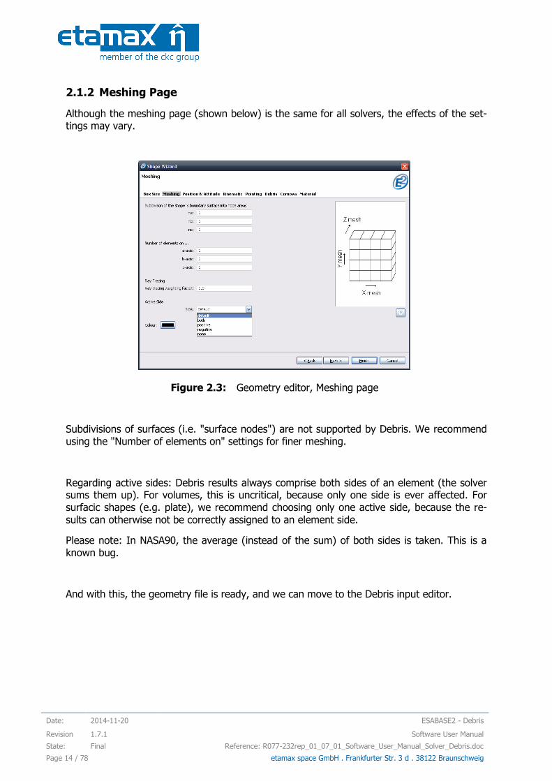
2.1.2 Meshing Page
Although the meshing page (shown below) is the same for all solvers, the effects of the set-tings may vary.
Figure 2.3: Geometry editor, Meshing page
Subdivisions of surfaces (i.e. "surface nodes") are not supported by Debris. We recommend using the "Number of elements on" settings for finer meshing.
Regarding active sides: Debris results always comprise both sides of an element (the solver sums them up). For volumes, this is uncritical, because only one side is ever affected. For surfacic shapes (e.g. plate), we recommend choosing only one active side, because the re-sults can otherwise not be correctly assigned to an element side.
Please note: In NASA90, the average (instead of the sum) of both sides is taken. This is a known bug.
And with this, the geometry file is ready, and we can move to the Debris input editor.
ESABASE2 - Debris Date: 2014-11-20
Software User Manual Revision: 1.7.1
Reference: R077-232rep_01_07_01_Software_User_Manual_Solver_Debris.doc State: Final
etamax space GmbH . Frankfurter Str. 3 d . 38122 Braunschweig Page 15 / 78
2.2 Debris Input
Complementing the Debris parameters bound to the geometry (see previous section), the global Debris/Meteoroid input parameters are all specified in the Debris input editor. This editor is divided into three tabs:
Debris Main Tab: Specifies the parameters for the geometrical analysis (see section 2.2.1).
Ground Test Tab: An efficient way to test damage equations (see section 2.2.2).
Non-Geometric Analysis Tab: Allows a fast guess for the expected flux values on a specific orbit (see section 2.2.3).
2.2.1 Debris Main Tab
The main tab of the Debris input editor contains four major blocks for specifying geometrical analysis input parameters:
Model selection: Allows you to choose among debris and meteoroid models, and to edit dedicated model parameters (see section 2.2.1.1).
Size boundaries: Limits on the type of debris or meteoroids to be considered in the analysis (see section 2.2.1.2).
Ray tracing: Defines the accuracy of ray tracing results (see section 2.2.1.3).
Damage Model: Defines a set of failure and damage equation combinations for the Debris analysis (see section 2.2.1.4).
Within the damage model block the option “user subroutine” can be selected. How to define your own damage equation in a Fortran library will be explained in section 2.2.1.5.

Date: 2014-11-20 ESABASE2 - Debris
Revision 1.7.1 Software User Manual
State: Final Reference: R077-232rep_01_07_01_Software_User_Manual_Solver_Debris.doc
Page 16 / 78 etamax space GmbH . Frankfurter Str. 3 d . 38122 Braunschweig
The figure below shows the ESABASE2/Debris main tab within the Debris input editor.
Figure 2.4: Debris input editor, main tab
At the bottom of the editor, you can see the "Debris", "Ground Test" and "Non-Geometric Analysis" tabs. This subsection is concerned with the main "Debris" tab.
In the following, the four sections of the main tab will be explained.
ESABASE2 - Debris Date: 2014-11-20
Software User Manual Revision: 1.7.1
Reference: R077-232rep_01_07_01_Software_User_Manual_Solver_Debris.doc State: Final
etamax space GmbH . Frankfurter Str. 3 d . 38122 Braunschweig Page 17 / 78
2.2.1.1 Model selection
Your first decision is which debris and meteoroid models you want to use. The following fig-ure shows the model selection block within the Debris main tab.
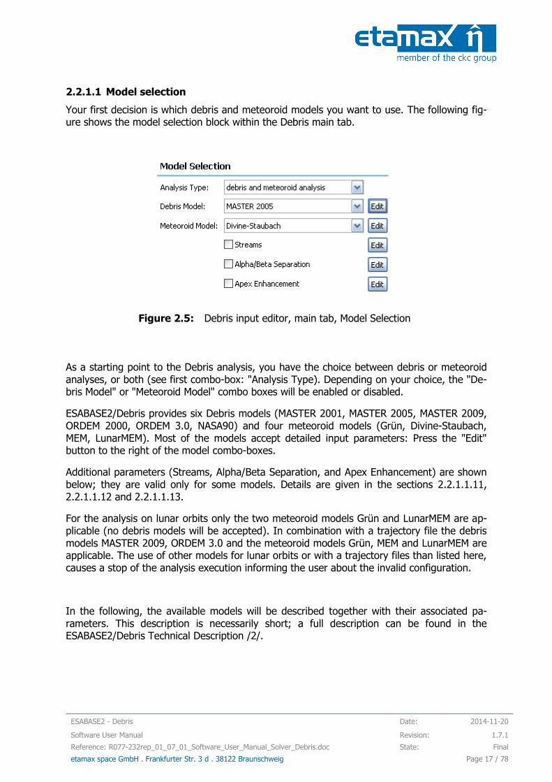
Figure 2.5: Debris input editor, main tab, Model Selection
As a starting point to the Debris analysis, you have the choice between debris or meteoroid analyses, or both (see first combo-box: "Analysis Type). Depending on your choice, the "De-bris Model" or "Meteoroid Model" combo boxes will be enabled or disabled.
ESABASE2/Debris provides six Debris models (MASTER 2001, MASTER 2005, MASTER 2009, ORDEM 2000, ORDEM 3.0, NASA90) and four meteoroid models (Grün, Divine-Staubach, MEM, LunarMEM). Most of the models accept detailed input parameters: Press the "Edit" button to the right of the model combo-boxes.
Additional parameters (Streams, Alpha/Beta Separation, and Apex Enhancement) are shown below; they are valid only for some models. Details are given in the sections 2.2.1.1.11, 2.2.1.1.12 and 2.2.1.1.13.
For the analysis on lunar orbits only the two meteoroid models Grün and LunarMEM are ap-plicable (no debris models will be accepted). In combination with a trajectory file the debris models MASTER 2009, ORDEM 3.0 and the meteoroid models Grün, MEM and LunarMEM are applicable. The use of other models for lunar orbits or with a trajectory files than listed here, causes a stop of the analysis execution informing the user about the invalid configuration.
In the following, the available models will be described together with their associated pa-rameters. This description is necessarily short; a full description can be found in the ESABASE2/Debris Technical Description /2/.

Date: 2014-11-20 ESABASE2 - Debris
Revision 1.7.1 Software User Manual
State: Final Reference: R077-232rep_01_07_01_Software_User_Manual_Solver_Debris.doc
Page 18 / 78 etamax space GmbH . Frankfurter Str. 3 d . 38122 Braunschweig
2.2.1.1.1 Debris model: MASTER 2001
MASTER 2001 /11/ is the 2001 version of ESA’s meteoroid and space debris reference model; it is the forerunner of MASTER 2005 (see next subsubsection). When you click on the "Edit" button, a dialog with MASTER 2001 input parameters will open, as shown in the fol-lowing figure.
Figure 2.6: Debris input editor, main tab, Model Selection, MASTER 2001
Apart from the assumed debris density (default: 2.8 g/cm3 as material mix average), the MASTER 2001 model is based on numerical modelling of various population sources, which can be included or excluded from an analysis.
Launch and mission related objects: payloads and satellites, upper stages, support structures. These are mostly larger, trackable objects.
o Note that the Westford needles experiment is included as subpopulation and cannot be turned off with this flag.
Fragments (collision and explosion) before reference epoch (2001-05-01): These are known fragment populations.
NaK droplet releases: coolant droplets released from Russian RORSAT satellites.
SRM (solid rocket motor) firing waste products:
o slag produced in the final firing phase, mostly > 1 mm
ESABASE2 - Debris Date: 2014-11-20
Software User Manual Revision: 1.7.1
Reference: R077-232rep_01_07_01_Software_User_Manual_Solver_Debris.doc State: Final
etamax space GmbH . Frankfurter Str. 3 d . 38122 Braunschweig Page 19 / 78
o Aluminium oxide (Al203) dust
Paint flakes are generated by surface degradation effects (mostly sunlight and ther-mal cycling)
Ejecta are small fragments of the S/C created by the impact of debris or meteoroids.
Collision (but not explosion) fragments after reference epoch; covers assumed colli-sion rate of satellites with other bodies in the future.
Explosion (but not collision) after reference epoch; covers assumed explosion rate of satellites in the future.
In the context of the MASTER 2001 model, "reference epoch" or "historic" means dates until 2001-05-01. The "future" are dates from 2001-05-01; note that from there, objects < 1 mm are not considered (this also means that paint flakes, ejecta and dust are not available, be-cause they are always < 1 mm).
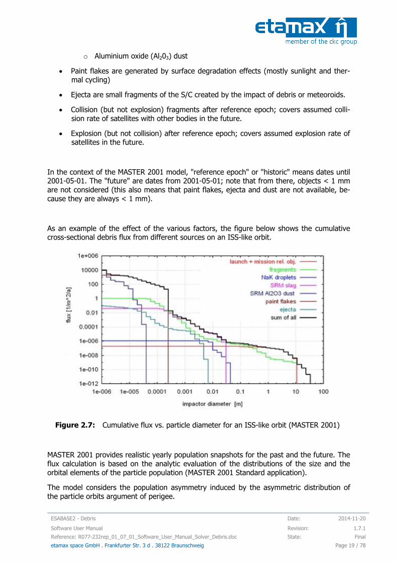
As an example of the effect of the various factors, the figure below shows the cumulative cross-sectional debris flux from different sources on an ISS-like orbit.
Figure 2.7: Cumulative flux vs. particle diameter for an ISS-like orbit (MASTER 2001)
MASTER 2001 provides realistic yearly population snapshots for the past and the future. The flux calculation is based on the analytic evaluation of the distributions of the size and the orbital elements of the particle population (MASTER 2001 Standard application).
The model considers the population asymmetry induced by the asymmetric distribution of the particle orbits argument of perigee.
Date: 2014-11-20 ESABASE2 - Debris
Revision 1.7.1 Software User Manual
State: Final Reference: R077-232rep_01_07_01_Software_User_Manual_Solver_Debris.doc
Page 20 / 78 etamax space GmbH . Frankfurter Str. 3 d . 38122 Braunschweig
MASTER 2001 covers the entire altitude range from LEO to GEO (150 km to 37000 km). Within the given altitude range there are no restrictions concerning the target orbit, so that highly eccentric orbits such as GTO can be analysed.
The MASTER population snapshots are available from year 1980 to 2020. Consequently, his-toric missions (e.g. LDEF) and future missions can be analysed using realistic population snapshots. The population snapshots of the May 1st of the mission start year are used for the analysis.
For the future evolution of the space debris environment the following assumptions have been applied:
continuation of space activity (launches, explosions, solid rocket motor firings) at the same rate as in the recent past,
no new satellite constellations deployed,
no implementation of debris mitigation measures.
This corresponds to the MASTER 2001 future reference scenario.

ESABASE2 - Debris Date: 2014-11-20
Software User Manual Revision: 1.7.1
Reference: R077-232rep_01_07_01_Software_User_Manual_Solver_Debris.doc State: Final
etamax space GmbH . Frankfurter Str. 3 d . 38122 Braunschweig Page 21 / 78
2.2.1.1.2 Debris model: MASTER 2005
MASTER 2005 /19/ is ESA’s meteoroid and space debris reference model, and the successor of MASTER 2001 (see previous subsubsection). When you click on the "Edit" button, a dialog with MASTER 2005 input parameters will open, as show in the following figure.
Figure 2.8: Debris input editor, main tab, Model Selection, MASTER 2005
The MASTER 2005 options are similar to the MASTER 2001 options (see previous subsubsec-tion). The following differences have to be noted:
Collision and explosion fragments cover both historic and future populations, not only historic populations as in MASTER 2001.
o This also explains why the "Fragments (historic)" option has vanished in com-parison to MASTER 2001.
Like MASTER 2001, MASTER 2005 covers altitudes from 186 km to 37000 km. The "future" is from 2005-05-01 and in the future; objects < 1 mm are not considered. The population snapshots of the May 1st of the mission start year are used for the analysis.

Date: 2014-11-20 ESABASE2 - Debris
Revision 1.7.1 Software User Manual
State: Final Reference: R077-232rep_01_07_01_Software_User_Manual_Solver_Debris.doc
Page 22 / 78 etamax space GmbH . Frankfurter Str. 3 d . 38122 Braunschweig
2.2.1.1.3 Debris model: MASTER 2009
MASTER 2009 /23/ is ESA’s meteoroid and space debris reference model, and the successor of MASTER 2005 (see previous subsubsection). When you click on the "Edit" button, a dialog with MASTER 2009 input parameters will open, as show in the following figure.
Figure 2.9: Debris input editor, main tab, Model Selection, MASTER 2009
The MASTER 2009 options are similar to the MASTER 2005 options (see previous subsubsec-tion). The following differences to MASTER 2005 have to be noted:
Objects down to 1 μm are considered for both the historic and the future populations (MASTER 2005 do not consider objects < 1 mm for future populations)
Both historic and future populations for solid rocket motor dust are available absence of the hint ‘historic populations only’.
Both historic and future populations for paint flakes are available absence of the hint ‘historic populations only’.
Both historic and future populations for ejecta are available absence of the hint ‘historic populations only’.
The new source multi layer insulation (MLI) is introduced. Historic populations until the reference date are provided for this source.
The reference date of MASTER 2009 is the 2009-05-01. Dates after the reference date are considered as “future”. MASTER 2009 covers altitudes from 186 km to ca. 37000 km. The population snapshots of the May 1st of the mission start year are used for the analysis.

ESABASE2 - Debris Date: 2014-11-20
Software User Manual Revision: 1.7.1
Reference: R077-232rep_01_07_01_Software_User_Manual_Solver_Debris.doc State: Final
etamax space GmbH . Frankfurter Str. 3 d . 38122 Braunschweig Page 23 / 78
2.2.1.1.4 Debris model: NASA90
NASA90 /16/ is an analytical debris model developed by NASA, which provides a simple and very fast debris flux calculation, but does not fully reflect the current knowledge of the Earth's debris environment, in particular the existence of a large number of particles on ec-centric orbits.
Upon clicking the "Edit" ( ) button, the NASA90 input parameters dialog is opened, as shown in the screenshot below.
Figure 2.10: Debris input editor, main tab, Model Selection, NASA90
As with all debris models, the average density of the debris material can be specified.
The debris mass (P) and fragments number (Q) annual growth rates are specified as per-centage, where 1 = 100% growth. It is recommended to use the default values.
Solar flux is used to specify the solar activity; appropriate values for the mission duration can e.g. be retrieved using the publicly available SWENET database /22/.
At the bottom, you see the debris velocity range, namely the minimum and maximum debris impact velocity to be considered. The default is from 0 to 20 km/s.
Please note that the NASA90 model is restricted to orbital altitudes below 1000km.

Date: 2014-11-20 ESABASE2 - Debris
Revision 1.7.1 Software User Manual
State: Final Reference: R077-232rep_01_07_01_Software_User_Manual_Solver_Debris.doc
Page 24 / 78 etamax space GmbH . Frankfurter Str. 3 d . 38122 Braunschweig
2.2.1.1.5 Debris model: ORDEM 2000
ORDEM2000 /15/ is a debris model developed by NASA; it is the successor of NASA96, which in turn followed NASA90. The model describes the orbital debris environment in the low earth orbit region between 200 km and 2000 km altitude.
The only user-editable input parameter is the assumed debris material density (default: 2.8 g/cm3), as shown in the figure below.
Figure 2.11: Debris input editor, main tab, model selection, ORDEM 2000
ORDEM 2000 is appropriate for engineering solutions requiring knowledge and estimates of the orbital debris environment (debris spatial density, flux, etc.). The model includes a large set of observational data (both in-situ and ground-based), covering the object size range from 10 µm to 10 m.
The analytical technique uses a maximum likelihood estimator to convert observations into debris population probability distribution functions; these functions then form the basis of the debris populations. A finite element model processes the debris populations to form the debris environment.
ESABASE2 - Debris Date: 2014-11-20
Software User Manual Revision: 1.7.1
Reference: R077-232rep_01_07_01_Software_User_Manual_Solver_Debris.doc State: Final
etamax space GmbH . Frankfurter Str. 3 d . 38122 Braunschweig Page 25 / 78
2.2.1.1.6 Debris model: ORDEM 3.0
ORDEM 3.0 /26/ is a space debris engineering model developed by NASA; it is the successor of ORDEM2000.
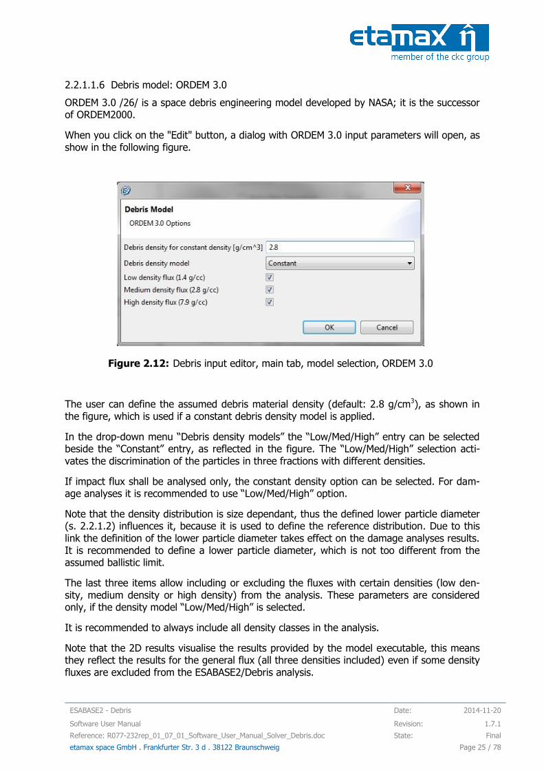
When you click on the "Edit" button, a dialog with ORDEM 3.0 input parameters will open, as show in the following figure.
Figure 2.12: Debris input editor, main tab, model selection, ORDEM 3.0
The user can define the assumed debris material density (default: 2.8 g/cm3), as shown in the figure, which is used if a constant debris density model is applied.
In the drop-down menu “Debris density models” the “Low/Med/High” entry can be selected beside the “Constant” entry, as reflected in the figure. The “Low/Med/High” selection acti-vates the discrimination of the particles in three fractions with different densities.
If impact flux shall be analysed only, the constant density option can be selected. For dam-age analyses it is recommended to use “Low/Med/High” option.
Note that the density distribution is size dependant, thus the defined lower particle diameter (s. 2.2.1.2) influences it, because it is used to define the reference distribution. Due to this link the definition of the lower particle diameter takes effect on the damage analyses results. It is recommended to define a lower particle diameter, which is not too different from the assumed ballistic limit.
The last three items allow including or excluding the fluxes with certain densities (low den-sity, medium density or high density) from the analysis. These parameters are considered only, if the density model “Low/Med/High” is selected.
It is recommended to always include all density classes in the analysis.
Note that the 2D results visualise the results provided by the model executable, this means they reflect the results for the general flux (all three densities included) even if some density fluxes are excluded from the ESABASE2/Debris analysis.

Date: 2014-11-20 ESABASE2 - Debris
Revision 1.7.1 Software User Manual
State: Final Reference: R077-232rep_01_07_01_Software_User_Manual_Solver_Debris.doc
Page 26 / 78 etamax space GmbH . Frankfurter Str. 3 d . 38122 Braunschweig
The ORDEM 3.0 model describes the orbital debris environment for the Earth orbits between 100 km and 40000 km altitude and for the time range between 2010 and 2035.
ORDEM 3.0 is appropriate for engineering solutions requiring knowledge and estimates of the orbital debris environment (debris spatial density, flux, etc.). The model includes a large set of observational data (both in-situ and ground-based), covering the object size range from 10 µm to 10 m.
The analytical technique uses the Bayesian statistical model for population derivation. A finite element model processes the debris populations to form the debris environment.
Note that the runtimes of ORDEM 3.0 can be very long, especially for higher eccentricities. They can last from some minutes for LEO and more than an hour for GTO like orbits. The progress can be seen in the console where ORDEM 3.0 is running. Please consider the run-times if you plan an analysis with ORDEM 3.0, especially if you use trajectory file, because then ORDEM 3.0 is executed for each orbital point individually.

ESABASE2 - Debris Date: 2014-11-20
Software User Manual Revision: 1.7.1
Reference: R077-232rep_01_07_01_Software_User_Manual_Solver_Debris.doc State: Final
etamax space GmbH . Frankfurter Str. 3 d . 38122 Braunschweig Page 27 / 78
2.2.1.1.7 Meteoroid model: Grün
Grün /14/ is an omni-directional interplanetary flux model for sporadic meteoroid environ-ment. It can be applied for Earth and lunar orbits. When you press the "Edit" button, a dia-log with the Grün input parameters shown in the figure below appears.
Figure 2.13: Debris input editor, main tab, Model Selection, Grün
On top, you see the meteoroid density option. Below, choose between this constant meteor-oid density and alternatively the NASA90 density distribution model (the latter choice will ignore your meteoroid density specification above).
The next two lines are concerned with the meteoroid velocity distribution option:
Constant meteoroid velocity; for this option, the default value is 17 km/s.
The NASA90 velocity distribution. In most cases, this delivers the best results, and is thus the recommended option for the industrial user. The NASA90 velocity distribu-tion is not applicable to lunar orbits, due to the intended design for Earth orbits.
The Taylor HRMP velocity distribution. This model is the most complex option. It is also applicable and recommended for the lunar orbits.
The last two lines handle the meteoroid velocity range, namely the minimum and maximum meteoroid velocity to be considered. The default is 11 km/s and 72 km/s.

Date: 2014-11-20 ESABASE2 - Debris
Revision 1.7.1 Software User Manual
State: Final Reference: R077-232rep_01_07_01_Software_User_Manual_Solver_Debris.doc
Page 28 / 78 etamax space GmbH . Frankfurter Str. 3 d . 38122 Braunschweig
2.2.1.1.8 Meteoroid model: Divine-Staubach
Divine-Staubach /13/ /18/ is a meteoroid model which is also part of the MASTER 2009 model. When you press the "Edit" button, a dialog shows the the Divine-Staubach input pa-rameters depicted in the screenshot below.
Figure 2.14: Debris input editor, main tab, Model Selection, Divine-Staubach
The only parameter is the material density of meteoroids. It is assumed to be constant.
Divine-Staubach is based on the size and orbital element distributions of five meteoroid sub-populations, and thus provides directional information in the same way as the MASTER 2009 debris model.

ESABASE2 - Debris Date: 2014-11-20
Software User Manual Revision: 1.7.1
Reference: R077-232rep_01_07_01_Software_User_Manual_Solver_Debris.doc State: Final
etamax space GmbH . Frankfurter Str. 3 d . 38122 Braunschweig Page 29 / 78
2.2.1.1.9 Meteoroid model: MEM
MEM /20/ is a meteoroid model developed by the University of Western Ontario, Canada. Upon pressing "Edit", a dialog with the MEM input parameters opens, as shown in the figure below.
Figure 2.15: Debris input editor, main tab, Model Selection, MEM
MEM has no options by itself, using a constant meteoroid density of 1 g/cm3. The option available here is used to convert mass to diameter for damage computation. We propose to always use 1 g/cm3.
Please note that the default 2.5 g/cm3 is fitting only for the other meteoroid models – all models use the same parameter within the data model; this is the reason that the default in the GUI cannot be 1 g/cm3.
MEM is a parametric model of the spatial distribution of sporadic meteoroids. The primary source is short-period comets with aphelia less than 7 AU. The model also considers the con-tributions from long-period comets to the sporadic meteor complex, and includes the effects of the gravitational shielding and focussing of the planets.
Date: 2014-11-20 ESABASE2 - Debris
Revision 1.7.1 Software User Manual
State: Final Reference: R077-232rep_01_07_01_Software_User_Manual_Solver_Debris.doc
Page 30 / 78 etamax space GmbH . Frankfurter Str. 3 d . 38122 Braunschweig
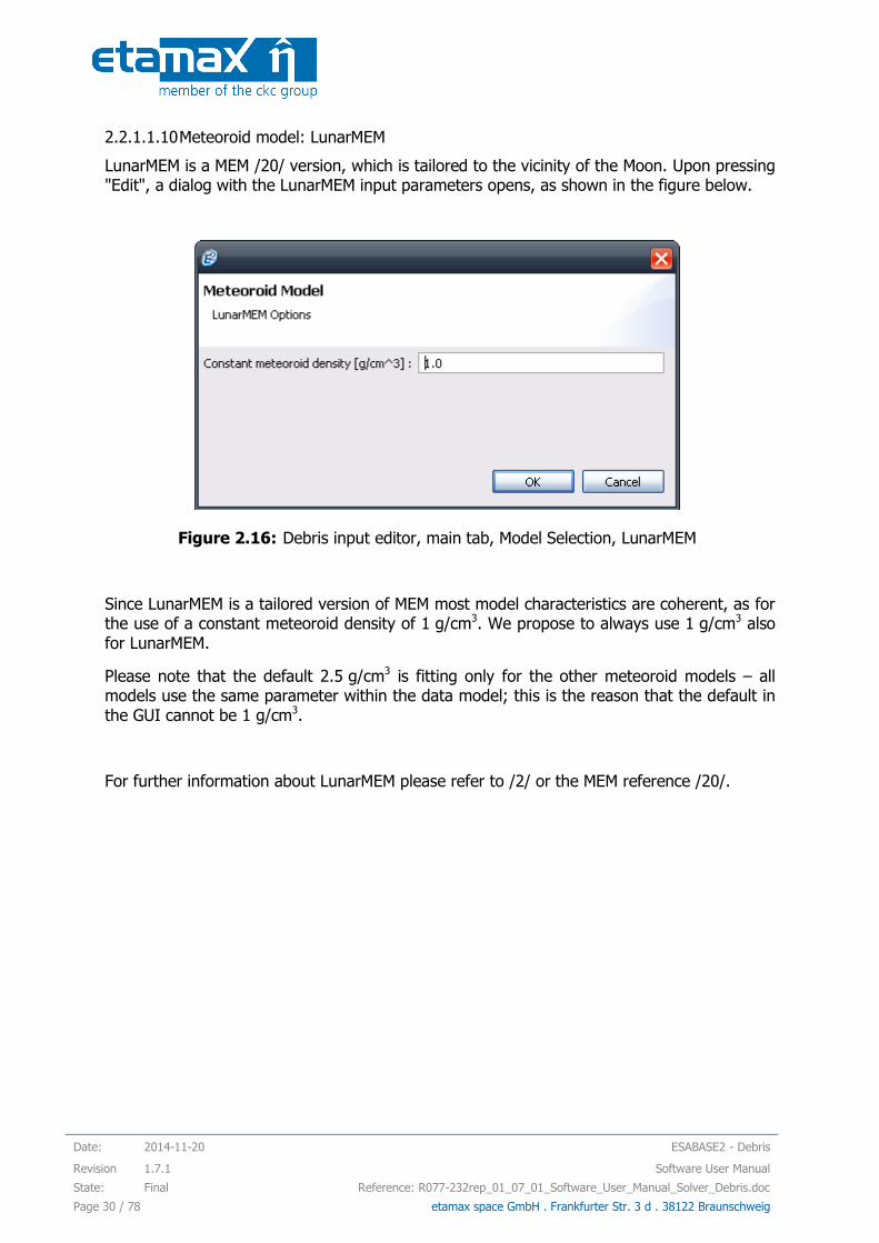
2.2.1.1.10 Meteoroid model: LunarMEM
LunarMEM is a MEM /20/ version, which is tailored to the vicinity of the Moon. Upon pressing "Edit", a dialog with the LunarMEM input parameters opens, as shown in the figure below.
Figure 2.16: Debris input editor, main tab, Model Selection, LunarMEM
Since LunarMEM is a tailored version of MEM most model characteristics are coherent, as for the use of a constant meteoroid density of 1 g/cm3. We propose to always use 1 g/cm3 also for LunarMEM.
Please note that the default 2.5 g/cm3 is fitting only for the other meteoroid models – all models use the same parameter within the data model; this is the reason that the default in the GUI cannot be 1 g/cm3.
For further information about LunarMEM please refer to /2/ or the MEM reference /20/.
ESABASE2 - Debris Date: 2014-11-20
Software User Manual Revision: 1.7.1
Reference: R077-232rep_01_07_01_Software_User_Manual_Solver_Debris.doc State: Final
etamax space GmbH . Frankfurter Str. 3 d . 38122 Braunschweig Page 31 / 78
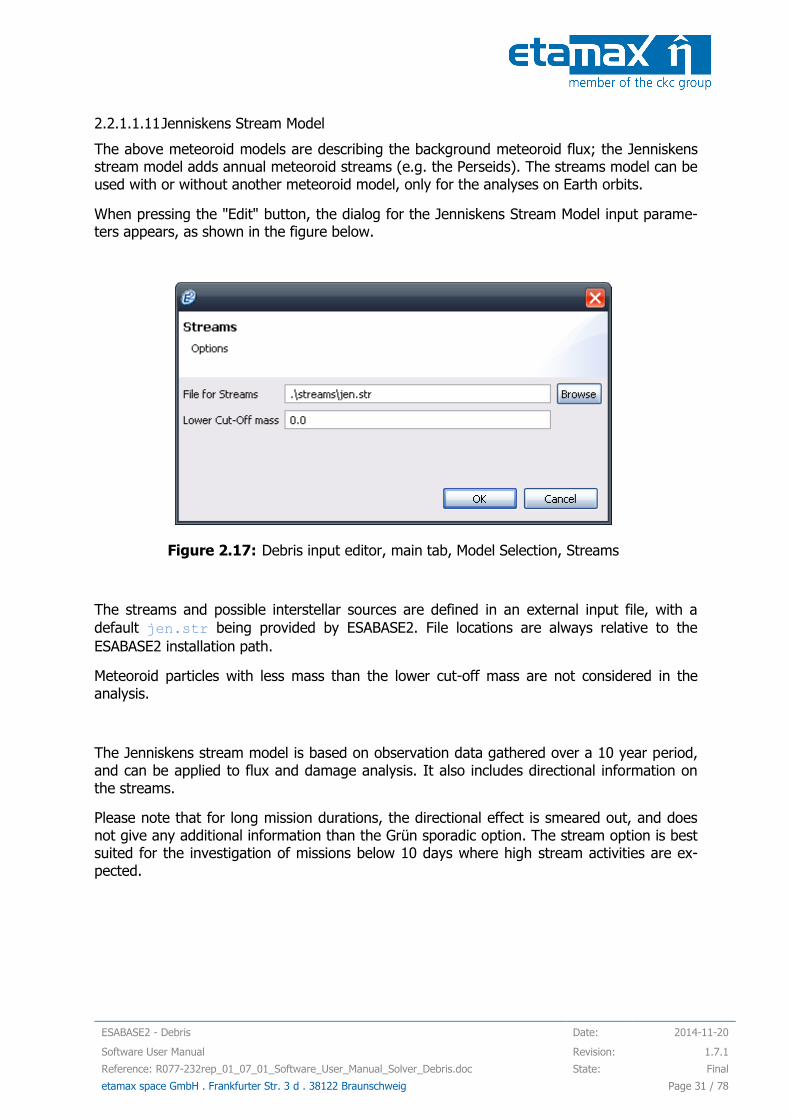
2.2.1.1.11 Jenniskens Stream Model
The above meteoroid models are describing the background meteoroid flux; the Jenniskens stream model adds annual meteoroid streams (e.g. the Perseids). The streams model can be used with or without another meteoroid model, only for the analyses on Earth orbits.
When pressing the "Edit" button, the dialog for the Jenniskens Stream Model input parame-ters appears, as shown in the figure below.
Figure 2.17: Debris input editor, main tab, Model Selection, Streams
The streams and possible interstellar sources are defined in an external input file, with a
default jen.str being provided by ESABASE2. File locations are always relative to the
ESABASE2 installation path.
Meteoroid particles with less mass than the lower cut-off mass are not considered in the analysis.
The Jenniskens stream model is based on observation data gathered over a 10 year period, and can be applied to flux and damage analysis. It also includes directional information on the streams.
Please note that for long mission durations, the directional effect is smeared out, and does not give any additional information than the Grün sporadic option. The stream option is best suited for the investigation of missions below 10 days where high stream activities are ex-pected.

Date: 2014-11-20 ESABASE2 - Debris
Revision 1.7.1 Software User Manual
State: Final Reference: R077-232rep_01_07_01_Software_User_Manual_Solver_Debris.doc
Page 32 / 78 etamax space GmbH . Frankfurter Str. 3 d . 38122 Braunschweig
2.2.1.1.12 Alpha-Beta Separation
As an improvement to the Grün meteoroid model, the Alpha-Beta Separation divides the me-teoroids in alpha particles (following the Grün sporadic omni-directional flux model) and smaller beta particles stemming from the sun.
When you press "Edit", the Alpha-Beta Separation options shown in the screenshot below appear in a dialog.
Figure 2.18: Debris input editor, main tab, Model Selection, Alpha-Beta Separation
The velocity distribution of the beta particles can be modified by specifying two parameters (for more details, see /10/):
V0: cross-over velocity; default: 20.0 km/s
Gamma (exponent); default: 0.18
The Alpha-Beta Separation obtains improved directional information by attempting to split off the beta meteoroids, which are driven away from the Sun into hyperbolic orbits by radiation pressure, from the alpha meteoroids. It is applicable only to Earth orbits.
An apex enhancement of the alpha meteoroids and interstellar streams (see next subsubsec-tion) may introduce further directional information.
We do not recommend using other values than the default values for this model, unless you have in-depth knowledge in astrophysics.

ESABASE2 - Debris Date: 2014-11-20
Software User Manual Revision: 1.7.1
Reference: R077-232rep_01_07_01_Software_User_Manual_Solver_Debris.doc State: Final
etamax space GmbH . Frankfurter Str. 3 d . 38122 Braunschweig Page 33 / 78
2.2.1.1.13 Apex Enhancement
As a modification to the Grün model, the Apex Enhancement describes the meteoroid flux enhancement caused by the earth's motion on its orbit around the sun (similar to the en-hanced flux a spacecraft experiences in velocity direction). It is applicable only to Earth or-bits.
If you press "Edit", a dialog shows the Apex Enhancement input parameters shown in the figure below.
Figure 2.19: Debris input editor, main tab, Model Selection, Apex Enhancement
Two parameters can be used to describe the ratio of flux and velocities between apex ("front") and antapex ("back") directions (see /10/ for more details):
RF: antapex to apex flux ratio; default: 2.0
Dv: velocity ratio; default: 0.36
As with Alpha-Beta Separation, we do not recommend using other values than the default values for this model, unless you have in-depth knowledge in astrophysics.
Date: 2014-11-20 ESABASE2 - Debris
Revision 1.7.1 Software User Manual
State: Final Reference: R077-232rep_01_07_01_Software_User_Manual_Solver_Debris.doc
Page 34 / 78 etamax space GmbH . Frankfurter Str. 3 d . 38122 Braunschweig
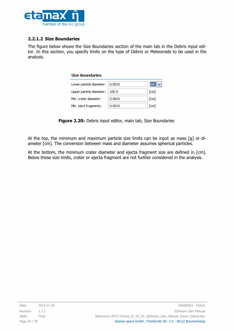
2.2.1.2 Size Boundaries
The figure below shows the Size Boundaries section of the main tab in the Debris input edi-tor. In this section, you specify limits on the type of Debris or Meteoroids to be used in the analysis.
Figure 2.20: Debris input editor, main tab, Size Boundaries
At the top, the minimum and maximum particle size limits can be input as mass [g] or di-ameter [cm]. The conversion between mass and diameter assumes spherical particles.
At the bottom, the minimum crater diameter and ejecta fragment size are defined in [cm]. Below these size limits, crater or ejecta fragment are not further considered in the analysis.

ESABASE2 - Debris Date: 2014-11-20
Software User Manual Revision: 1.7.1
Reference: R077-232rep_01_07_01_Software_User_Manual_Solver_Debris.doc State: Final
etamax space GmbH . Frankfurter Str. 3 d . 38122 Braunschweig Page 35 / 78
2.2.1.3 Ray Tracing
Ray tracing is the primary technique in ESABASE2 to determine whether Debris or Meteor-oids hit the spacecraft geometry at a specific orbital point. Below, you can see a screenshot of the Ray Tracing section in the main tab.
Figure 2.21: Debris input editor, main tab, Ray Tracing
The "Primary rays" parameter governs the number of primary rays to be fired per element. For ESABASE geometric models, at least 250 rays per element are recommended, for non-geometric analyses 1000 rays.
In the middle, the "Secondary rays" parameter specifies the number of secondary rays to be fired from each impact point. Due to the high computational effort caused by this option it is recommended to choose fairly low values (< 100).
Another option to reduce computation time is to specify a “Secondary ray jump” which causes the program to skip the respective number of secondary rays.
Date: 2014-11-20 ESABASE2 - Debris
Revision 1.7.1 Software User Manual
State: Final Reference: R077-232rep_01_07_01_Software_User_Manual_Solver_Debris.doc
Page 36 / 78 etamax space GmbH . Frankfurter Str. 3 d . 38122 Braunschweig
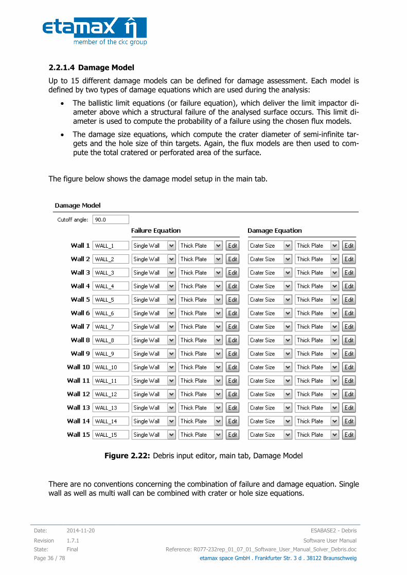
2.2.1.4 Damage Model
Up to 15 different damage models can be defined for damage assessment. Each model is defined by two types of damage equations which are used during the analysis:
The ballistic limit equations (or failure equation), which deliver the limit impactor di-ameter above which a structural failure of the analysed surface occurs. This limit di-ameter is used to compute the probability of a failure using the chosen flux models.
The damage size equations, which compute the crater diameter of semi-infinite tar-gets and the hole size of thin targets. Again, the flux models are then used to com-pute the total cratered or perforated area of the surface.
The figure below shows the damage model setup in the main tab.
Figure 2.22: Debris input editor, main tab, Damage Model
There are no conventions concerning the combination of failure and damage equation. Single wall as well as multi wall can be combined with crater or hole size equations.
ESABASE2 - Debris Date: 2014-11-20
Software User Manual Revision: 1.7.1
Reference: R077-232rep_01_07_01_Software_User_Manual_Solver_Debris.doc State: Final
etamax space GmbH . Frankfurter Str. 3 d . 38122 Braunschweig Page 37 / 78
Failure and damage equations of the ESABASE2/Debris analysis tool are defined in a para-metric form, with editable parameters (constants and exponents). The parameters can be edited via the “Edit” buttons shown in Figure 2.22.
Up to seven entities can be defined:
for failure equation:
the single wall ballistic limit equation
the multiple wall ballistic limit equation and
the user subroutine parameters
for damage equation:
the crater size equation
the parametric clear hole equation
the advanced hole equation and
the user subroutine parameters.
The user subroutine option is only for expert users with Fortran and/or C++ experience (see section 2.2.1.5).
For a detailed description of the user input of the damage equations, please refer to /10/.
Date: 2014-11-20 ESABASE2 - Debris
Revision 1.7.1 Software User Manual
State: Final Reference: R077-232rep_01_07_01_Software_User_Manual_Solver_Debris.doc
Page 38 / 78 etamax space GmbH . Frankfurter Str. 3 d . 38122 Braunschweig
2.2.1.5 User Subroutine
For expert users of the original ESABASE, the possibility to use your own damage equation subroutine is provided. This option requires the availability of a FORTRAN or C/C++ compiler and linker.
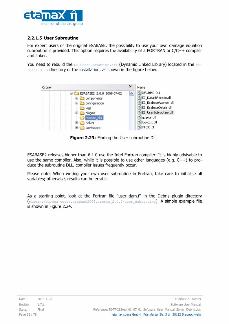
You need to rebuild the E2_UserSubroutine.dll (Dynamic Linked Library) located in the re-
lease_dlls directory of the installation, as shown in the figure below.
Figure 2.23: Finding the User subroutine DLL
ESABASE2 releases higher than 6.1.0 use the Intel Fortran compiler. It is highly advisable to use the same compiler. Also, while it is possible to use other languages (e.g. C++) to pro-duce the subroutine DLL, compiler issues frequently occur.
Please note: When writing your own user subroutine in Fortran, take care to initialise all variables; otherwise, results can be erratic.
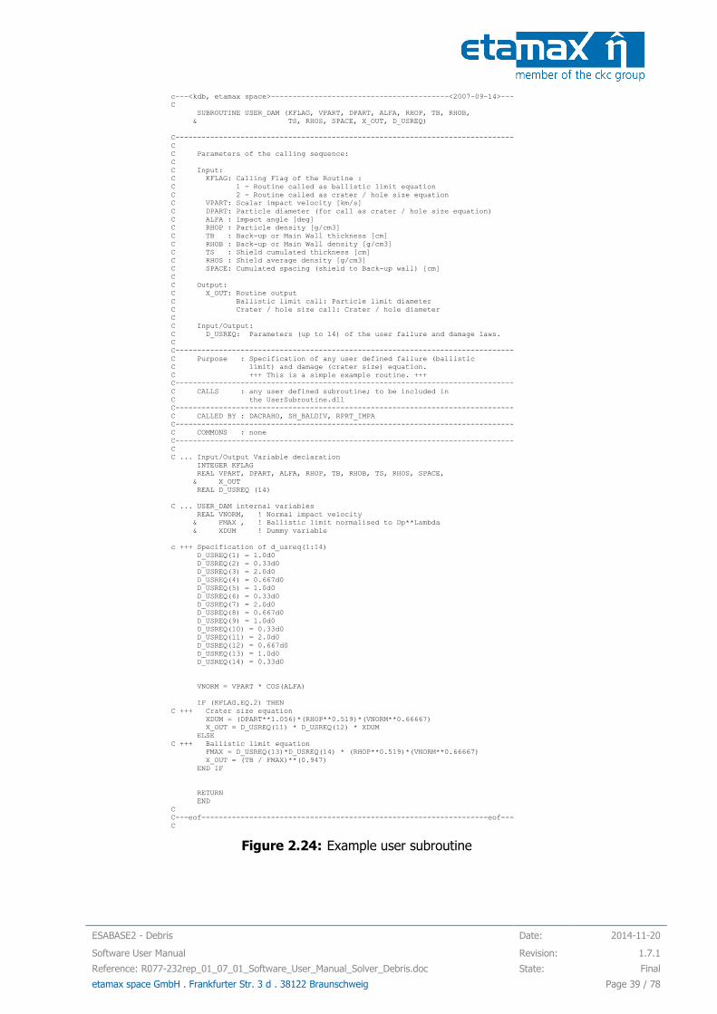
As a starting point, look at the Fortran file "user_dam.f" in the Debris plugin directory
(plugins\eu.esa.estec.esabase2005.debris_2.0.0\user_subroutine). A simple example file
is shown in Figure 2.24.
ESABASE2 - Debris Date: 2014-11-20
Software User Manual Revision: 1.7.1
Reference: R077-232rep_01_07_01_Software_User_Manual_Solver_Debris.doc State: Final
etamax space GmbH . Frankfurter Str. 3 d . 38122 Braunschweig Page 39 / 78
c---<kdb, etamax space>-----------------------------------------<2007-09-14>---
C
SUBROUTINE USER_DAM (KFLAG, VPART, DPART, ALFA, RHOP, TB, RHOB,
& TS, RHOS, SPACE, X_OUT, D_USREQ)
C------------------------------------------------------------------------------
C
C Parameters of the calling sequence:
C
C Input:
C KFLAG: Calling Flag of the Routine :
C 1 - Routine called as ballistic limit equation
C 2 - Routine called as crater / hole size equation
C VPART: Scalar impact velocity [km/s]
C DPART: Particle diameter (for call as crater / hole size equation)
C ALFA : Impact angle [deg]
C RHOP : Particle density [g/cm3]
C TB : Back-up or Main Wall thickness [cm]
C RHOB : Back-up or Main Wall density [g/cm3]
C TS : Shield cumulated thickness [cm]
C RHOS : Shield average density [g/cm3]
C SPACE: Cumulated spacing (shield to Back-up wall) [cm]
C
C Output:
C X_OUT: Routine output
C Ballistic limit call: Particle limit diameter
C Crater / hole size call: Crater / hole diameter
C
C Input/Output:
C D_USREQ: Parameters (up to 14) of the user failure and damage laws.
C
C------------------------------------------------------------------------------
C Purpose : Specification of any user defined failure (ballistic
C limit) and damage (crater size) equation.
C +++ This is a simple example routine. +++
C------------------------------------------------------------------------------
C CALLS : any user defined subroutine; to be included in
C the UserSubroutine.dll
C------------------------------------------------------------------------------
C CALLED BY : DACRAHO, SH_BALDIV, RPRT_IMPA
C------------------------------------------------------------------------------
C COMMONS : none
C------------------------------------------------------------------------------
C
C ... Input/Output Variable declaration
INTEGER KFLAG
REAL VPART, DPART, ALFA, RHOP, TB, RHOB, TS, RHOS, SPACE,
& X_OUT
REAL D_USREQ (14)
C ... USER_DAM internal variables
REAL VNORM, ! Normal impact velocity
& FMAX , ! Ballistic limit normalised to Dp**Lambda
& XDUM ! Dummy variable
c +++ Specification of d_usreq(1:14)
D_USREQ(1) = 1.0d0
D_USREQ(2) = 0.33d0
D_USREQ(3) = 2.0d0
D_USREQ(4) = 0.667d0
D_USREQ(5) = 1.0d0
D_USREQ(6) = 0.33d0
D_USREQ(7) = 2.0d0
D_USREQ(8) = 0.667d0
D_USREQ(9) = 1.0d0
D_USREQ(10) = 0.33d0
D_USREQ(11) = 2.0d0
D_USREQ(12) = 0.667d0
D_USREQ(13) = 1.0d0
D_USREQ(14) = 0.33d0
VNORM = VPART * COS(ALFA)
IF (KFLAG.EQ.2) THEN
C +++ Crater size equation
XDUM = (DPART**1.056)*(RHOP**0.519)*(VNORM**0.66667)
X_OUT = D_USREQ(11) * D_USREQ(12) * XDUM
ELSE
C +++ Ballistic limit equation
FMAX = D_USREQ(13)*D_USREQ(14) * (RHOP**0.519)*(VNORM**0.66667)
X_OUT = (TB / FMAX)**(0.947)
END IF
RETURN
END
C
C---eof------------------------------------------------------------------eof---
C
Figure 2.24: Example user subroutine

Date: 2014-11-20 ESABASE2 - Debris
Revision 1.7.1 Software User Manual
State: Final Reference: R077-232rep_01_07_01_Software_User_Manual_Solver_Debris.doc
Page 40 / 78 etamax space GmbH . Frankfurter Str. 3 d . 38122 Braunschweig
After the variables specification, a block containing 14 parameters can be defined for the user damage equation.
The user sub-routine must be named user_dam.f.
The flag KFLAG indicates how the subroutine is called. When user_dam is called with KFLAG =
1, it is to be used as a ballistic limit equation, if KFLAG = 2, it is to be used as a crater / hole
equation. Thus one subroutine can cover both types of equation.
It is possible to add further subroutines in the file user_dam.f which are called by the main
user subroutine USER_DAM. Thus, the advanced user can build his own library of damage
equations.
In case of persisting issues, please contact the ESABASE2 development team using the email address provided on the website /3/.
To apply the subroutine to the entire model, choose "User Subroutine" as damage equation in the Debris input editor, as described above (subsection 2.2.1.4). To apply it only to parts of the S/C geometry, go to the geometry editor, modify a shape via wizard, and on the De-bris page, choose "User Subroutine" as shield type (see also section 2.1).

ESABASE2 - Debris Date: 2014-11-20
Software User Manual Revision: 1.7.1
Reference: R077-232rep_01_07_01_Software_User_Manual_Solver_Debris.doc State: Final
etamax space GmbH . Frankfurter Str. 3 d . 38122 Braunschweig Page 41 / 78
2.2.2 Debris Ground Test Tab
At the bottom of the Debris input editor, the second tab leads to the "Ground Test" page, which is depicted in the figure below.
Figure 2.25: Debris input editor, Ground Test tab
The ground test option enables you to run the damage equations on their own, outside of the ESABASE2/Debris analysis; its purpose is to test and preview the results of the damage equations.
The following sections are available:
Ground Test: Choose damage type (ballistic limit or crater size) and shielding type (Wall_1 to Wall_15). To define the wall configuration see section 2.2.1.4.
Shielding Parameters: Choose shield thickness and density (and spacing in case of double walls).
Input Parameters: Impact angle, density, velocity and diameter can be specified ei-ther as single values or as arrays of values. Each variable has three parameters: the minimum value, the maximum value and the number of steps. For single shots, only the minimum parameter is used. For tabled data, when the variable is used as x-axis or y-curve parameter, all three parameters are used.
Visualisation: Choose the axis on the result graph.
Unlike the normal Debris analyses, the ground test can be performed directly within the De-bris input editor; for this purpose, press the "Run" button. Afterwards, the "Graph" and "Ta-ble" buttons at the bottom right are enabled, leading to the popup windows illustrated in the screenshot below.

Date: 2014-11-20 ESABASE2 - Debris
Revision 1.7.1 Software User Manual
State: Final Reference: R077-232rep_01_07_01_Software_User_Manual_Solver_Debris.doc
Page 42 / 78 etamax space GmbH . Frankfurter Str. 3 d . 38122 Braunschweig
Figure 2.26: Debris input editor, Ground Test tab, Run
Graph and table show the same results.
ESABASE2 - Debris Date: 2014-11-20
Software User Manual Revision: 1.7.1
Reference: R077-232rep_01_07_01_Software_User_Manual_Solver_Debris.doc State: Final
etamax space GmbH . Frankfurter Str. 3 d . 38122 Braunschweig Page 43 / 78
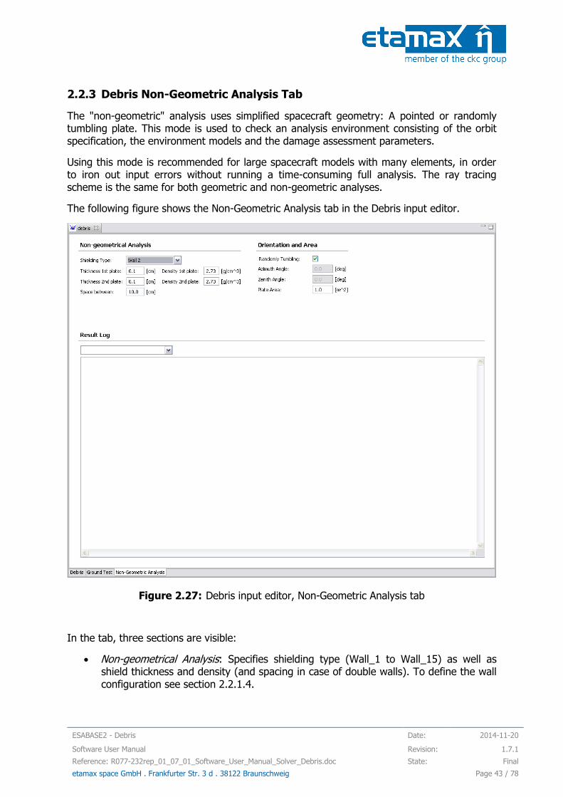
2.2.3 Debris Non-Geometric Analysis Tab
The "non-geometric" analysis uses simplified spacecraft geometry: A pointed or randomly tumbling plate. This mode is used to check an analysis environment consisting of the orbit specification, the environment models and the damage assessment parameters.
Using this mode is recommended for large spacecraft models with many elements, in order to iron out input errors without running a time-consuming full analysis. The ray tracing scheme is the same for both geometric and non-geometric analyses.
The following figure shows the Non-Geometric Analysis tab in the Debris input editor.
Figure 2.27: Debris input editor, Non-Geometric Analysis tab
In the tab, three sections are visible:
Non-geometrical Analysis: Specifies shielding type (Wall_1 to Wall_15) as well as shield thickness and density (and spacing in case of double walls). To define the wall configuration see section 2.2.1.4.

Date: 2014-11-20 ESABASE2 - Debris
Revision 1.7.1 Software User Manual
State: Final Reference: R077-232rep_01_07_01_Software_User_Manual_Solver_Debris.doc
Page 44 / 78 etamax space GmbH . Frankfurter Str. 3 d . 38122 Braunschweig
Orientation and area: Specifies the plate size and its orientation or randomly tumbling property.
Result Log: Execution log of the analysis run (former listing file).
2.2.3.1 Non-Geometrical Analysis
The following screenshot shows the Non-Geometrical Analysis section for single (left) and multi wall (right) selection.
Figure 2.28: Debris input editor, Non-Geometric Analysis tab, Single and Multi wall
The input values correspond to the ones used in the geometry editor, in the Debris page of the shape wizards (see 2.1).
2.2.3.2 Plate Orientation and Area
The figure below shows the Plate Orientation and Area section within the Non-Geometric Analysis tab.
Figure 2.29: Debris input editor, Non-Geometric Analysis tab, Orientation and Area
ESABASE2 - Debris Date: 2014-11-20
Software User Manual Revision: 1.7.1
Reference: R077-232rep_01_07_01_Software_User_Manual_Solver_Debris.doc State: Final
etamax space GmbH . Frankfurter Str. 3 d . 38122 Braunschweig Page 45 / 78
The plate orientation can be one of the following.
Randomly tumbling: This is the random tumbling plate (RTP) mode. It often corre-sponds to the environment models themselves, and is an effective way to get a quick first-order assessment of the micro-particle environment risk for a mission.
Oriented: For this mode, azimuth and zenith angles of the plate normal can be de-fined.
o The azimuth angle is the angle with respect to the velocity direction (0 deg corresponds to the ram direction, positive towards right).
o The zenith angle is the angle to the space (zenith) direction (0 deg corre-sponds to the space direction).
Please note that if the zenith angle is zero degree, the azimuth angle is irrelevant and the normal vector points in the space direction. The azimuth angle rotates the plate then only around the axis to nadir but due to the equal plate sides, this is irrelevant.
In both cases, the area of the plate can be defined. Normally the default (1 m2) is used, but a specific area can be specified instead, e.g. in case of a detector or other special surface.
2.2.3.3 Result Log
The results of a non-geometrical analysis are displayed in the bottom part of the Debris input editor. You can select between four different sets of results:
hits vs. crater size
debris and meteoroid flux and damage results
failures vs. ballistic limit
orbit propagation results
All results will be presented in textual form (ASCII files).
The results listings are also available in the .\ListingFiles folder of the corresponding project directory. The names of the listing files are composed from the string ‘NonGeom’, the analy-sis date and time and the type of listing (result set).
2.3 Debris Analysis
With both debris information within the spacecraft geometry and global debris input parame-ters specified, the time has come to perform a debris analysis. There are two types of analy-sis runs:
Date: 2014-11-20 ESABASE2 - Debris
Revision 1.7.1 Software User Manual
State: Final Reference: R077-232rep_01_07_01_Software_User_Manual_Solver_Debris.doc
Page 46 / 78 etamax space GmbH . Frankfurter Str. 3 d . 38122 Braunschweig
Geometric Analysis: This is what you would normally expect: A mission and a space-craft geometry are sent to orbit propagation and debris analysis (see section 2.3.1).
Non-geometric Analysis: Subtracts the S/C geometry from the analysis, instead taking a simple plate (see section 2.3.2).
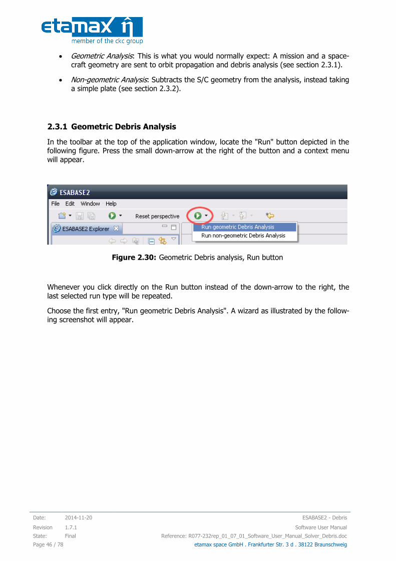
2.3.1 Geometric Debris Analysis
In the toolbar at the top of the application window, locate the "Run" button depicted in the following figure. Press the small down-arrow at the right of the button and a context menu will appear.
Figure 2.30: Geometric Debris analysis, Run button
Whenever you click directly on the Run button instead of the down-arrow to the right, the last selected run type will be repeated.
Choose the first entry, "Run geometric Debris Analysis". A wizard as illustrated by the follow-ing screenshot will appear.
ESABASE2 - Debris Date: 2014-11-20
Software User Manual Revision: 1.7.1
Reference: R077-232rep_01_07_01_Software_User_Manual_Solver_Debris.doc State: Final
etamax space GmbH . Frankfurter Str. 3 d . 38122 Braunschweig Page 47 / 78
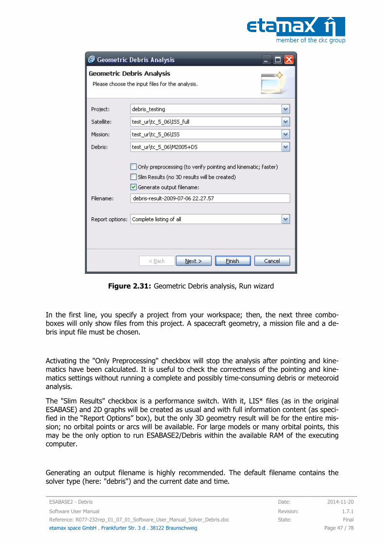
Figure 2.31: Geometric Debris analysis, Run wizard
In the first line, you specify a project from your workspace; then, the next three combo-boxes will only show files from this project. A spacecraft geometry, a mission file and a de-bris input file must be chosen.
Activating the "Only Preprocessing" checkbox will stop the analysis after pointing and kine-matics have been calculated. It is useful to check the correctness of the pointing and kine-matics settings without running a complete and possibly time-consuming debris or meteoroid analysis.
The "Slim Results" checkbox is a performance switch. With it, LIS* files (as in the original ESABASE) and 2D graphs will be created as usual and with full information content (as speci-fied in the “Report Options” box), but the only 3D geometry result will be for the entire mis-sion; no orbital points or arcs will be available. For large models or many orbital points, this may be the only option to run ESABASE2/Debris within the available RAM of the executing computer.
Generating an output filename is highly recommended. The default filename contains the solver type (here: "debris") and the current date and time.

Date: 2014-11-20 ESABASE2 - Debris
Revision 1.7.1 Software User Manual
State: Final Reference: R077-232rep_01_07_01_Software_User_Manual_Solver_Debris.doc
Page 48 / 78 etamax space GmbH . Frankfurter Str. 3 d . 38122 Braunschweig
At the bottom, the "Report options" combo-box allows you to specify the content of the "Deb Met" listing (formerly *.LISD, *.LISM, *.LISDM output files) within the Debris result file. You can choose between the following options:
Output of a summary of objects: results on orbital arc and mission level, and on ob-ject and spacecraft level (no object/element summary, no orbital point related results and no element related results).
Output of header and summary all: the same, but including object/element summary and element related results.
Complete listing of objects: orbital point, orbital arc and mission related results on ob-ject and spacecraft level (no object/element summary, and no element related re-sults).
Complete listing of all: the same, but including object/element summary and element related results.
Optionally, you can press the "Next" button to go to the second page of the Debris analysis wizard, which is depicted in the figure below.
Figure 2.32: Geometric Debris analysis, Run dialog, export page
ESABASE2 - Debris Date: 2014-11-20
Software User Manual Revision: 1.7.1
Reference: R077-232rep_01_07_01_Software_User_Manual_Solver_Debris.doc State: Final
etamax space GmbH . Frankfurter Str. 3 d . 38122 Braunschweig Page 49 / 78
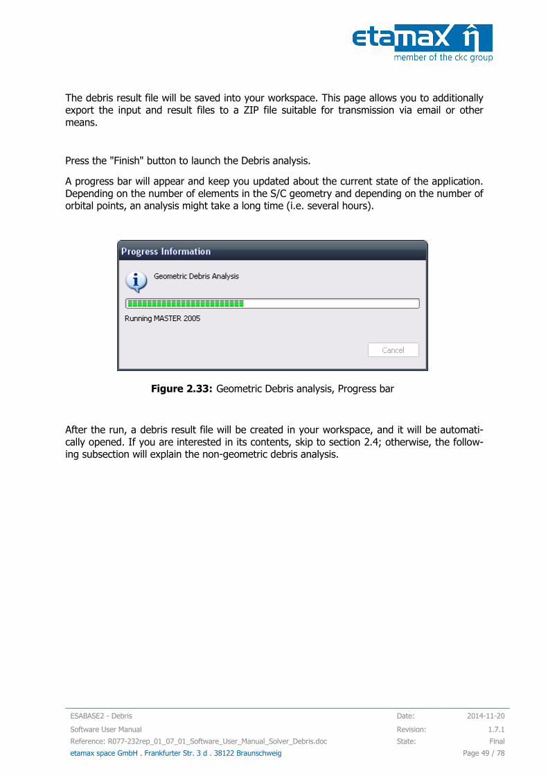
The debris result file will be saved into your workspace. This page allows you to additionally export the input and result files to a ZIP file suitable for transmission via email or other means.
Press the "Finish" button to launch the Debris analysis.
A progress bar will appear and keep you updated about the current state of the application. Depending on the number of elements in the S/C geometry and depending on the number of orbital points, an analysis might take a long time (i.e. several hours).
Figure 2.33: Geometric Debris analysis, Progress bar
After the run, a debris result file will be created in your workspace, and it will be automati-cally opened. If you are interested in its contents, skip to section 2.4; otherwise, the follow-ing subsection will explain the non-geometric debris analysis.

Date: 2014-11-20 ESABASE2 - Debris
Revision 1.7.1 Software User Manual
State: Final Reference: R077-232rep_01_07_01_Software_User_Manual_Solver_Debris.doc
Page 50 / 78 etamax space GmbH . Frankfurter Str. 3 d . 38122 Braunschweig
2.3.2 Non-geometric Debris Analysis
The non-geometric analysis uses a simple plate instead of a full spacecraft geometry; it is therefore considerably faster. As in the geometric debris analysis, locate the Run button and, this time, choose "Run non-geometric Debris Analysis".
The following figure shows the Run wizard for the non-geometric debris analysis.
Figure 2.34: Non-geometric Debris analysis, Run wizard
Compared to the geometric Debris analysis, this wizard is considerably simpler. The space-craft geometry input file is omitted and all options have been removed; only the report op-tions remain.
No output file needs to be specified since the result listings are displayed in the "Result Log" section of the Debris input editor’s "Non Geometric Analysis" tab. The content of the listings is stored within the debris input file.

ESABASE2 - Debris Date: 2014-11-20
Software User Manual Revision: 1.7.1
Reference: R077-232rep_01_07_01_Software_User_Manual_Solver_Debris.doc State: Final
etamax space GmbH . Frankfurter Str. 3 d . 38122 Braunschweig Page 51 / 78
The screenshot below shows the debris input editor, supplied with results from a non-geometrical debris analysis.
Figure 2.35: Non-geometric Debris analysis, results
In the "Result Log" section, the combo-box toggles between the output files, while the text area below shows the content of the selected file. Here, the Debris/Meteoroid listing ("LISTINGDEBMET") is shown.

Date: 2014-11-20 ESABASE2 - Debris
Revision 1.7.1 Software User Manual
State: Final Reference: R077-232rep_01_07_01_Software_User_Manual_Solver_Debris.doc
Page 52 / 78 etamax space GmbH . Frankfurter Str. 3 d . 38122 Braunschweig
2.4 Debris Results
A geometric Debris analysis produces a debris result file, which is interpreted by the Debris result editor. The editor contains the following functionalities:
3D Results: Shows the spacecraft geometry overlaid with the impact flux or other output parameters (see section 2.4.1).
2D Results: Graphs with different data about flux distributions at the orbital points as well as average flux distributions (see section 2.4.2).
Listings: In tradition of the original ESABASE, this tab shows the LIS* files produced by the Debris solver (see section 2.4.3).
Notes: A blank text area for your own notes (see section 2.4.4).
2.4.1 3D Results
The following figure shows the "3D Results" tab in a debris result editor.
Figure 2.36: Debris result editor, 3D Results
You can see a spacecraft geometry (Landsat7) with total impact flux, visualised by colour codes on the elements and decoded by the colour scale on the right. At the top of the editor, the same toolbar as in the geometry editor appears, allowing you to zoom, rotate and scroll around the spacecraft.
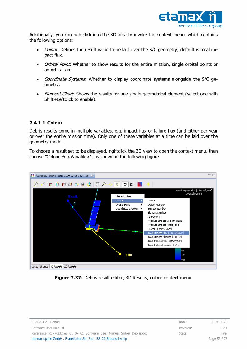
ESABASE2 - Debris Date: 2014-11-20
Software User Manual Revision: 1.7.1
Reference: R077-232rep_01_07_01_Software_User_Manual_Solver_Debris.doc State: Final
etamax space GmbH . Frankfurter Str. 3 d . 38122 Braunschweig Page 53 / 78
Additionally, you can rightclick into the 3D area to invoke the context menu, which contains the following options:
Colour: Defines the result value to be laid over the S/C geometry; default is total im-pact flux.
Orbital Point: Whether to show results for the entire mission, single orbital points or an orbital arc.
Coordinate Systems: Whether to display coordinate systems alongside the S/C ge-ometry.
Element Chart: Shows the results for one single geometrical element (select one with Shift+Leftclick to enable).
2.4.1.1 Colour
Debris results come in multiple variables, e.g. impact flux or failure flux (and either per year or over the entire mission time). Only one of these variables at a time can be laid over the geometry model.
To choose a result set to be displayed, rightclick the 3D view to open the context menu, then
choose "Colour <Variable>", as shown in the following figure.
Figure 2.37: Debris result editor, 3D Results, colour context menu
Date: 2014-11-20 ESABASE2 - Debris
Revision 1.7.1 Software User Manual
State: Final Reference: R077-232rep_01_07_01_Software_User_Manual_Solver_Debris.doc
Page 54 / 78 etamax space GmbH . Frankfurter Str. 3 d . 38122 Braunschweig
The first 4 items (listed below) are not part of the Debris results; instead they are used to gain an overview of the spacecraft geometry, and particular its objects, surfaces and ele-ments.
Colour: Displays exactly the same object colour which was used in the geometry edi-tor.
Object Number: Each object is identified by an object number. In this overlay, this object number is mapped to colours.
o Leftclick on an object in the 3D view to select it, and then look at the colour scale to the right. The appropriate colour will be marked, and the object num-ber will be shown.
Surface Number: Breaking down the objects, each surface is shown in a different col-our.
o Ctrl+leftclick on a surface in the 3D view to select it. The respective surface number is marked in the colour scale to the right.
Element Number: Further breaking down the surfaces, each element is shown in a different colour.
o Shift+leftclick on an element in the 3D view. The selected element number and color will be marked in the color scale.
The following 8 items show the respective quantity (listed below) as colours on the elements of the geometry model. To see the exact value on an element, Shift+leftclick the element; the colour scale on the right will then show the quantity value.
KS Factor
Average Impact Velocity [km/s]
Average Impact Angle [deg]
Crater Flux [%/year]
Total Impact Flux [1/m^2/year]
Total Impact Fluence [1/m^2]
Total Failure Flux [1/m^2/year]
Total Failure Fluence [1/m^2]
If the secondary ejecta option was activated in the Debris input editor, it is now additionally possible to display the direct impact/failure flux/fluence and the ejecta impact/failure flux/fluence.
Please note that results always sum up both sides of all elements. A distinction between positive and negative side of an element is not possible.
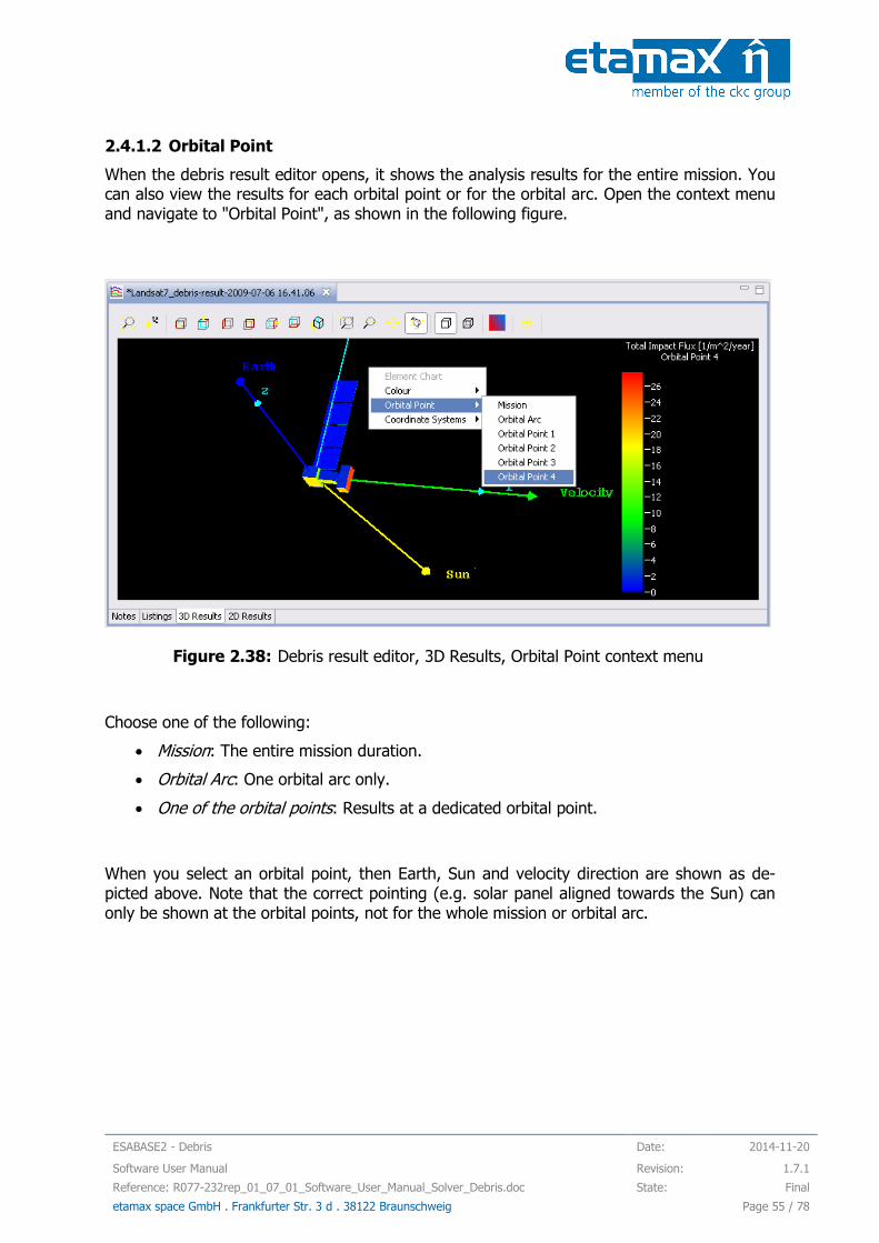
ESABASE2 - Debris Date: 2014-11-20
Software User Manual Revision: 1.7.1
Reference: R077-232rep_01_07_01_Software_User_Manual_Solver_Debris.doc State: Final
etamax space GmbH . Frankfurter Str. 3 d . 38122 Braunschweig Page 55 / 78
2.4.1.2 Orbital Point
When the debris result editor opens, it shows the analysis results for the entire mission. You can also view the results for each orbital point or for the orbital arc. Open the context menu and navigate to "Orbital Point", as shown in the following figure.
Figure 2.38: Debris result editor, 3D Results, Orbital Point context menu
Choose one of the following:
Mission: The entire mission duration.
Orbital Arc: One orbital arc only.
One of the orbital points: Results at a dedicated orbital point.
When you select an orbital point, then Earth, Sun and velocity direction are shown as de-picted above. Note that the correct pointing (e.g. solar panel aligned towards the Sun) can only be shown at the orbital points, not for the whole mission or orbital arc.

Date: 2014-11-20 ESABASE2 - Debris
Revision 1.7.1 Software User Manual
State: Final Reference: R077-232rep_01_07_01_Software_User_Manual_Solver_Debris.doc
Page 56 / 78 etamax space GmbH . Frankfurter Str. 3 d . 38122 Braunschweig
2.4.1.3 Coordinate Systems
To visualise the coordinate system you used in the geometry editor, change the coordinate system by opening the context menu and navigating to "Coordinate Systems", as shown in the following figure.
Figure 2.39: Debris result editor, 3D Results, Coordinate Systems context menu
You can choose among the following coordinate system settings:
No coordinates: Note that pointing vectors will also be deactivated.
Global coordinate system (centred): Shows the xyz-axis for the entire system.
Global coordinate system in the corner: Same as before, but in the corner of the sys-tem, not centred.
Global and local coordinate systems: Shows xyz-axis for each object. Detailed but probably slightly irritating for complex S/C geometries.

ESABASE2 - Debris Date: 2014-11-20
Software User Manual Revision: 1.7.1
Reference: R077-232rep_01_07_01_Software_User_Manual_Solver_Debris.doc State: Final
etamax space GmbH . Frankfurter Str. 3 d . 38122 Braunschweig Page 57 / 78
2.4.1.4 Element Chart
Different 2D graphs of the debris results can be shown for the entire spacecraft geometry using the "2D Charts" tab, as described in the next section (2.4.2). However it is also possi-ble to show graphs of only one element.
Shift+Leftclick an element of the S/C geometry, then open the context menu and select "Element Chart". The following figure shows the resulting small popup window.
Figure 2.40: Debris result editor, 3D Results, Element Chart
From the "Result Set" combo-box, select a variable; the appropriate graph for the given ele-ment will be displayed, as shown on the right. These are the same values that are colour coded in the element in the 3D view.
You also have the possibility to adjust the appearance of the graph via the “Options” button or a context menu opening on rightclicking, and to export the image as PNG or JPG via the “Export Image” button (s. sections 2.4.2.1and 2.4.2.2 for details).
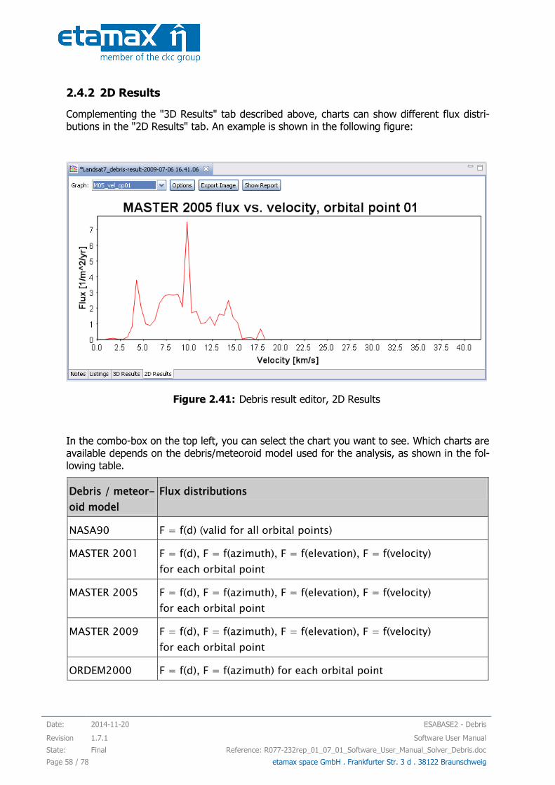
Date: 2014-11-20 ESABASE2 - Debris
Revision 1.7.1 Software User Manual
State: Final Reference: R077-232rep_01_07_01_Software_User_Manual_Solver_Debris.doc
Page 58 / 78 etamax space GmbH . Frankfurter Str. 3 d . 38122 Braunschweig
2.4.2 2D Results
Complementing the "3D Results" tab described above, charts can show different flux distri-butions in the "2D Results" tab. An example is shown in the following figure:
Figure 2.41: Debris result editor, 2D Results
In the combo-box on the top left, you can select the chart you want to see. Which charts are available depends on the debris/meteoroid model used for the analysis, as shown in the fol-lowing table.
Debris / meteor-
oid model
Flux distributions
NASA90 F = f(d) (valid for all orbital points)
MASTER 2001 F = f(d), F = f(azimuth), F = f(elevation), F = f(velocity)
for each orbital point
MASTER 2005 F = f(d), F = f(azimuth), F = f(elevation), F = f(velocity)
for each orbital point
MASTER 2009 F = f(d), F = f(azimuth), F = f(elevation), F = f(velocity)
for each orbital point
ORDEM2000 F = f(d), F = f(azimuth) for each orbital point
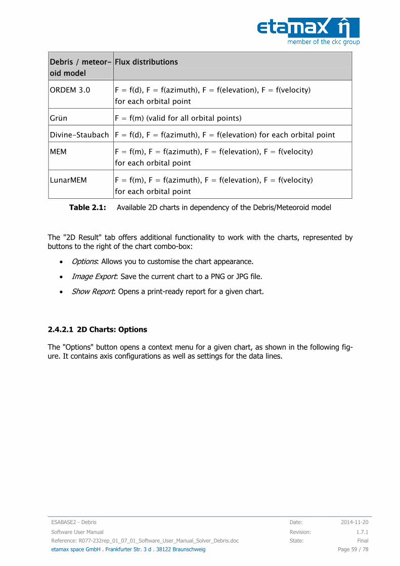
ESABASE2 - Debris Date: 2014-11-20
Software User Manual Revision: 1.7.1
Reference: R077-232rep_01_07_01_Software_User_Manual_Solver_Debris.doc State: Final
etamax space GmbH . Frankfurter Str. 3 d . 38122 Braunschweig Page 59 / 78
Debris / meteor-
oid model
Flux distributions
ORDEM 3.0 F = f(d), F = f(azimuth), F = f(elevation), F = f(velocity)
for each orbital point
Grün F = f(m) (valid for all orbital points)
Divine-Staubach F = f(d), F = f(azimuth), F = f(elevation) for each orbital point
MEM F = f(m), F = f(azimuth), F = f(elevation), F = f(velocity)
for each orbital point
LunarMEM F = f(m), F = f(azimuth), F = f(elevation), F = f(velocity)
for each orbital point
Table 2.1: Available 2D charts in dependency of the Debris/Meteoroid model
The "2D Result" tab offers additional functionality to work with the charts, represented by buttons to the right of the chart combo-box:
Options: Allows you to customise the chart appearance.
Image Export: Save the current chart to a PNG or JPG file.
Show Report: Opens a print-ready report for a given chart.
2.4.2.1 2D Charts: Options
The "Options" button opens a context menu for a given chart, as shown in the following fig-ure. It contains axis configurations as well as settings for the data lines.
Date: 2014-11-20 ESABASE2 - Debris
Revision 1.7.1 Software User Manual
State: Final Reference: R077-232rep_01_07_01_Software_User_Manual_Solver_Debris.doc
Page 60 / 78 etamax space GmbH . Frankfurter Str. 3 d . 38122 Braunschweig
Figure 2.42: Debris result editor, 2D Results, options
You can customize the following chart properties:
x, y axis
o Label Text: Changes the text of the axis label.
o Grid: Displays horizontal/vertical dashed lines.
o Label font, Label font size, Label font style: Changes the appearance of the axis label.
o Maximum, Minimum: The value range that this chart shows
o Number format: The format of the number labels, e.g. the number of decimal places, can be specified.
o Number scaling: Choose between linear or logarithmic scale.
Title
o Graph title: The title text above the chart.
o Title visible: Show or hide the title text.
o Title Font, Title Font Size, Title Font Style: The appearance of the title text.
Legend
o Legend: Show or hide the legend.
o Legend Font, Legend Font Size, Legend Font Style: The appearance of the legend.
Background: The background color of the chart.
Box: Shows or hides the box around the graph.
ESABASE2 - Debris Date: 2014-11-20
Software User Manual Revision: 1.7.1
Reference: R077-232rep_01_07_01_Software_User_Manual_Solver_Debris.doc State: Final
etamax space GmbH . Frankfurter Str. 3 d . 38122 Braunschweig Page 61 / 78
Axis and label colour: The colour of the axis lines and the labels.
Major tick labels: Shows or hides number labels at the major ticks.
Minor tick marks: Display small ticks between the major ticks.
Ratio: Set a fixed aspect ratio.
Auto scaling: Re-scales the chart.
Graph Type: Choose between line-, bar- and scatter chart.
Series <num>:
o Linecolour, Linewidth: Color and width of the line of this data series.
o Stroke: Type of the line of this data series.
Range: Set the X and Y range that the chart covers.
2.4.2.2 2D Charts: Image Export
Pressing the "Export Image" button opens a file dialog asking for a location to save to. PNG and JPG format are possible. The size of the image is the same as it is currently shown; re-size the application window to get other image sizes.

Date: 2014-11-20 ESABASE2 - Debris
Revision 1.7.1 Software User Manual
State: Final Reference: R077-232rep_01_07_01_Software_User_Manual_Solver_Debris.doc
Page 62 / 78 etamax space GmbH . Frankfurter Str. 3 d . 38122 Braunschweig
2.4.2.3 2D Charts: Show Report
The chart can be embedded into a print-ready report; press the "Show Report" button to invoke it. After a dialog asking for a comment line has been confirmed, a report as shown in the following figure will appear in a popup window.
Figure 2.43: Debris result editor, 2D Results, reporting
This report details the chart properties and below the chart itself, followed by the data val-ues represented in the chart (on the second and following pages). It is thus a complete data description of a value pair's relation, suitable for distribution to your colleagues.
You may either print the report (press the print button) or choose "Export Save as PDF" for electronic distribution.
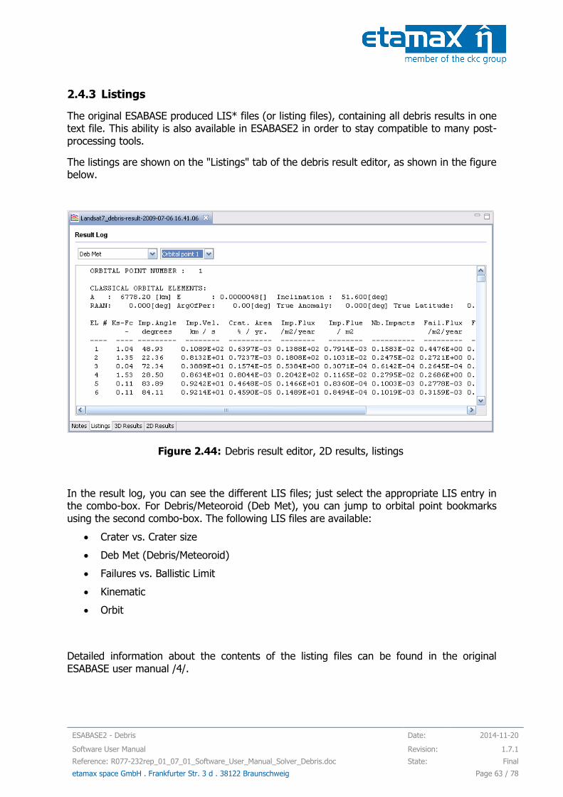
ESABASE2 - Debris Date: 2014-11-20
Software User Manual Revision: 1.7.1
Reference: R077-232rep_01_07_01_Software_User_Manual_Solver_Debris.doc State: Final
etamax space GmbH . Frankfurter Str. 3 d . 38122 Braunschweig Page 63 / 78
2.4.3 Listings
The original ESABASE produced LIS* files (or listing files), containing all debris results in one text file. This ability is also available in ESABASE2 in order to stay compatible to many post-processing tools.
The listings are shown on the "Listings" tab of the debris result editor, as shown in the figure below.
Figure 2.44: Debris result editor, 2D results, listings
In the result log, you can see the different LIS files; just select the appropriate LIS entry in the combo-box. For Debris/Meteoroid (Deb Met), you can jump to orbital point bookmarks using the second combo-box. The following LIS files are available:
Crater vs. Crater size
Deb Met (Debris/Meteoroid)
Failures vs. Ballistic Limit
Kinematic
Orbit
Detailed information about the contents of the listing files can be found in the original ESABASE user manual /4/.

Date: 2014-11-20 ESABASE2 - Debris
Revision 1.7.1 Software User Manual
State: Final Reference: R077-232rep_01_07_01_Software_User_Manual_Solver_Debris.doc
Page 64 / 78 etamax space GmbH . Frankfurter Str. 3 d . 38122 Braunschweig
Please note: The listing files are foremost saved as data nodes in the debris result file. Addi-tionally, they are written in ASCII format to the "Listings" subfolder of the current project folder, in order to be more easily accessible to post-processing tools.
Due to some confusion in the past the interpretation of the Crater vs. Crater size LIS file is described in the following section.
2.4.3.1 Crater vs. Crater size
The Figure 2.45 shows an example of a Crater vs. Crater size LIS file. The name indicates that it tabulates the number of craters again a crater size. The results are cumulative.
Figure 2.45: Example of Crater vs. Crater size LIS file.
The first column “IELMT” lists the elements of the model, thus the results of the Crater vs. Crater size LIS file are on the element level. The corresponding results on the object level are presented on the bottom of the Deb Met LIS file. Both LIS files provide the mission level of hits.
The second column lists the areas of the corresponding elements in [m²].
The columns 3 to 9 provide results (number of hits) for seven different crater size thresh-olds. This means the listed hit causes a crater that is equal or larger than the threshold cra-ter size. The first (minimum) threshold is the Min. crater diameter defined by the user, see 2.2.1.2. Based on this value the other six thresholds are defined by raising the crater size threshold by one order of magnitude. This can be seen very well in the first line of the table in Figure 2.45, which lists the values of the thresholds as head of the columns.
In the same way the LIS file Failures vs. Ballistic Limit can be interpreted. In this case the number of failures (instead of number of craters) is tabulated again the ‘ballistic limit’ (in-stead of crater size), which means thickness of the (back) wall. It uses the same principle and definition of the thresholds.
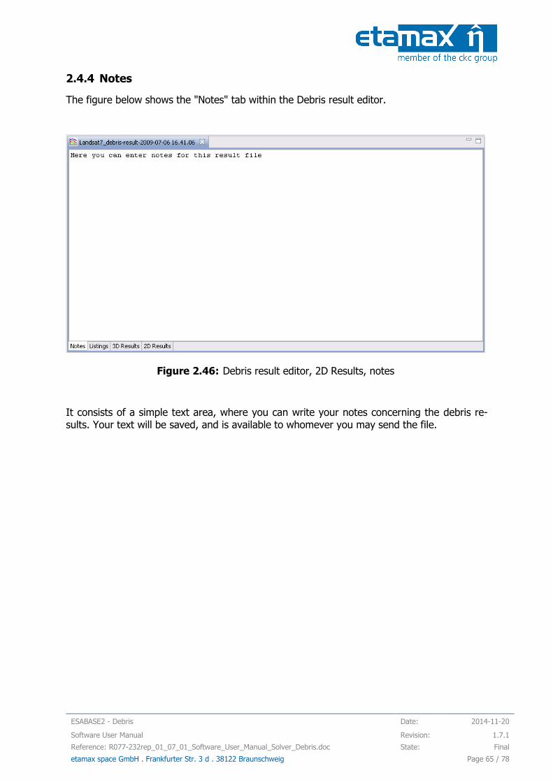
ESABASE2 - Debris Date: 2014-11-20
Software User Manual Revision: 1.7.1
Reference: R077-232rep_01_07_01_Software_User_Manual_Solver_Debris.doc State: Final
etamax space GmbH . Frankfurter Str. 3 d . 38122 Braunschweig Page 65 / 78
2.4.4 Notes
The figure below shows the "Notes" tab within the Debris result editor.
Figure 2.46: Debris result editor, 2D Results, notes
It consists of a simple text area, where you can write your notes concerning the debris re-sults. Your text will be saved, and is available to whomever you may send the file.

Date: 2014-11-20 ESABASE2 - Debris
Revision 1.7.1 Software User Manual
State: Final Reference: R077-232rep_01_07_01_Software_User_Manual_Solver_Debris.doc
Page 66 / 78 etamax space GmbH . Frankfurter Str. 3 d . 38122 Braunschweig
3 Lunar Mission Debris Analysis
The intention of this chapter is to provide a small overview how a debris analysis for lunar mission can be performed.
Figure 3.1: Scheme of the lunar mission of Chandrayaan 1 (source: North East India News)
The Figure 3.1 displays an example of a trajectory of a lunar mission, as was used for Chandrayaan 1.
3.1 Lunar Mission
Two different approaches can be used for an analysis of a lunar mission:
Abstraction of the mission by splitting it into multiple orbits;
Describing the mission with state vectors provided via a trajectory file.
In the first case the results of the individual orbits have to be post-processed manually to obtain the results for the whole mission.
The second case provides complete mission results. In this case, a trajectory file is used, describing the whole mission with up to 100 orbital points.
Both approaches for the mission definition are described in more detail in the following sec-tions.

ESABASE2 - Debris Date: 2014-11-20
Software User Manual Revision: 1.7.1
Reference: R077-232rep_01_07_01_Software_User_Manual_Solver_Debris.doc State: Final
etamax space GmbH . Frankfurter Str. 3 d . 38122 Braunschweig Page 67 / 78
3.1.1 Abstraction of the Lunar Mission
A lunar mission can be abstracted by the definition of multiple orbits. The simplest case in-cludes three orbits (only the journey from Earth to Moon):
A low Earth orbit (LEO), which is often called the parking orbit;
A highly elliptical orbit (HEO), the transfer orbit, with a perigee at the parking orbit and the apogee at the orbit of the Moon;
A low lunar orbit (LLO), which is the target orbit of the mission.
Each of the orbits represents one of the phases of a lunar mission. The three phases de-scribe roughly the lunar mission; the first phase includes the mission time in the vicinity of the Earth, here it is represented by a LEO. The second phase is the transfer from Earth to Moon, represented by a HEO. The third phase of the mission is the motion of the S/C in the vicinity of the Moon, in this case a LLO.
The individual orbits generated in the following give only an outlook of possible tracks and are not combined to reflect a real mission. To abstract a real mission the used mission ep-ochs and durations have to fit a meaningful timeline, i.e. the mission epochs have to form a continuous time interval (second track starts at the end of the first track etc.). Furthermore the start epoch and orbit parameters of the transfer orbit have to be defined in a way that the Moon interferes with the transfer orbit and the S/C is at the according sector of the orbit at the particular moment. This implies also the usage of the correct orbital parameters, e.g. inclination, true anomaly at start etc.
Nevertheless, to get an impression of the result magnitudes to be expected and to get the feeling of the usage, three independent orbits can be used. This is also the case for the fol-lowing orbit descriptions.
3.1.1.1 The Parking Orbit
Before the start of the journey to Moon the spacecraft is placed in an orbit around the Earth. A possibility is the low Earth orbit of the ISS. The basic values of such an orbit can be:
Central body (centre of motion): Earth
Semi-major axis = 6785 km
Eccentricity = 0.001
Inclination = 51.6 deg
Other angles = 0.0 deg
The mission starts on January the 1, 2013 at 0:00. The orbital period of the orbit is ca. 92.7 minutes, let’s say that 3 orbits are completed before starting the transfer, which means a mission duration of 278.1 minutes for the LEO. Thus the end epoch is January the 1, 2013 at 4:38 and 6 seconds.
The mission file can be created as described in /1/ section 3.1. The filename ParkingOrbit will be used in the text to identify the orbit. Figure 3.2 shows the mission editor with the parameters applied as introduced before.
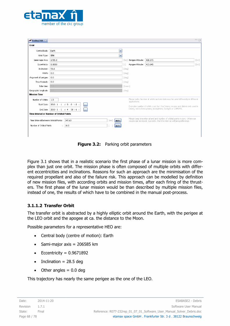
Date: 2014-11-20 ESABASE2 - Debris
Revision 1.7.1 Software User Manual
State: Final Reference: R077-232rep_01_07_01_Software_User_Manual_Solver_Debris.doc
Page 68 / 78 etamax space GmbH . Frankfurter Str. 3 d . 38122 Braunschweig
Figure 3.2: Parking orbit parameters
Figure 3.1 shows that in a realistic scenario the first phase of a lunar mission is more com-plex than just one orbit. The mission phase is often composed of multiple orbits with differ-ent eccentricities and inclinations. Reasons for such an approach are the minimisation of the required propellant and also of the failure risk. This approach can be modelled by definition of new mission files, with according orbits and mission times, after each firing of the thrust-ers. The first phase of the lunar mission would be than described by multiple mission files, instead of one, the results of which have to be combined in the manual post-process.
3.1.1.2 Transfer Orbit
The transfer orbit is abstracted by a highly elliptic orbit around the Earth, with the perigee at the LEO orbit and the apogee at ca. the distance to the Moon.
Possible parameters for a representative HEO are:
Central body (centre of motion): Earth
Sami-major axis = 206585 km
Eccentricity = 0.9671892
Inclination = 28.5 deg
Other angles = 0.0 deg
This trajectory has nearly the same perigee as the one of the LEO.
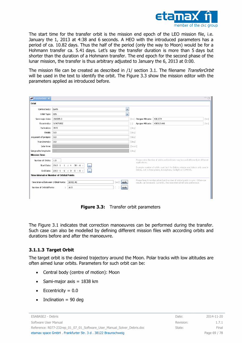
ESABASE2 - Debris Date: 2014-11-20
Software User Manual Revision: 1.7.1
Reference: R077-232rep_01_07_01_Software_User_Manual_Solver_Debris.doc State: Final
etamax space GmbH . Frankfurter Str. 3 d . 38122 Braunschweig Page 69 / 78
The start time for the transfer orbit is the mission end epoch of the LEO mission file, i.e. January the 1, 2013 at 4:38 and 6 seconds. A HEO with the introduced parameters has a period of ca. 10.82 days. Thus the half of the period (only the way to Moon) would be for a Hohmann transfer ca. 5.41 days. Let’s say the transfer duration is more than 5 days but shorter than the duration of a Hohmann transfer. The end epoch for the second phase of the lunar mission, the transfer is thus arbitrary adjusted to January the 6, 2013 at 0:00.
The mission file can be created as described in /1/ section 3.1. The filename TransferOrbit will be used in the text to identify the orbit. The Figure 3.3 show the mission editor with the parameters applied as introduced before.
Figure 3.3: Transfer orbit parameters
The Figure 3.1 indicates that correction manoeuvres can be performed during the transfer. Such case can also be modelled by defining different mission files with according orbits and durations before and after the manoeuvre.
3.1.1.3 Target Orbit
The target orbit is the desired trajectory around the Moon. Polar tracks with low altitudes are often aimed lunar orbits. Parameters for such orbit can be:
Central body (centre of motion): Moon
Sami-major axis = 1838 km
Eccentricity = 0.0
Inclination = 90 deg
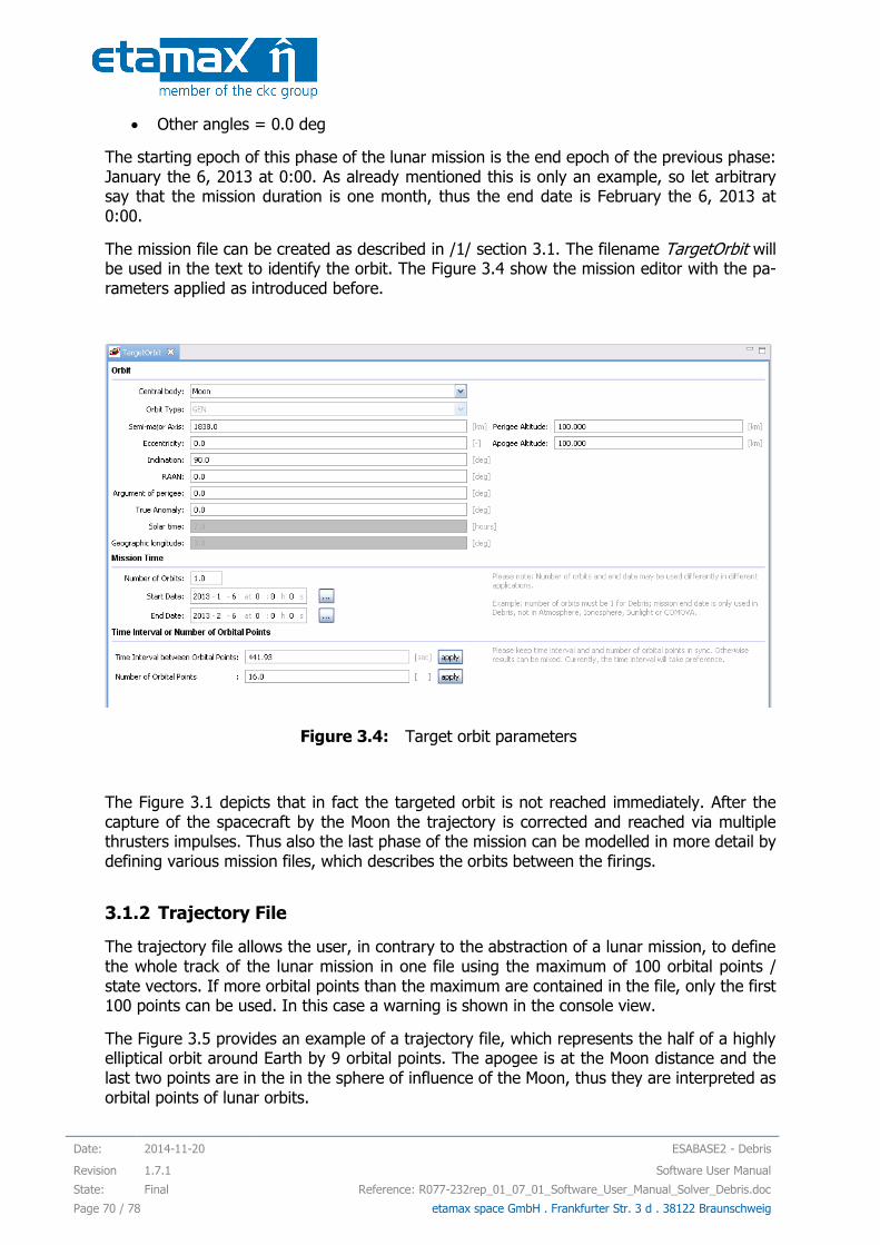
Date: 2014-11-20 ESABASE2 - Debris
Revision 1.7.1 Software User Manual
State: Final Reference: R077-232rep_01_07_01_Software_User_Manual_Solver_Debris.doc
Page 70 / 78 etamax space GmbH . Frankfurter Str. 3 d . 38122 Braunschweig
Other angles = 0.0 deg
The starting epoch of this phase of the lunar mission is the end epoch of the previous phase: January the 6, 2013 at 0:00. As already mentioned this is only an example, so let arbitrary say that the mission duration is one month, thus the end date is February the 6, 2013 at 0:00.
The mission file can be created as described in /1/ section 3.1. The filename TargetOrbit will be used in the text to identify the orbit. The Figure 3.4 show the mission editor with the pa-rameters applied as introduced before.
Figure 3.4: Target orbit parameters
The Figure 3.1 depicts that in fact the targeted orbit is not reached immediately. After the capture of the spacecraft by the Moon the trajectory is corrected and reached via multiple thrusters impulses. Thus also the last phase of the mission can be modelled in more detail by defining various mission files, which describes the orbits between the firings.
3.1.2 Trajectory File
The trajectory file allows the user, in contrary to the abstraction of a lunar mission, to define the whole track of the lunar mission in one file using the maximum of 100 orbital points / state vectors. If more orbital points than the maximum are contained in the file, only the first 100 points can be used. In this case a warning is shown in the console view.
The Figure 3.5 provides an example of a trajectory file, which represents the half of a highly elliptical orbit around Earth by 9 orbital points. The apogee is at the Moon distance and the last two points are in the in the sphere of influence of the Moon, thus they are interpreted as orbital points of lunar orbits.
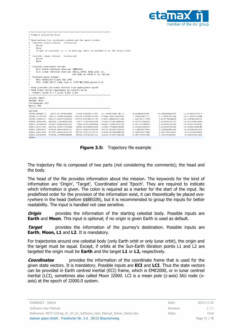
ESABASE2 - Debris Date: 2014-11-20
Software User Manual Revision: 1.7.1
Reference: R077-232rep_01_07_01_Software_User_Manual_Solver_Debris.doc State: Final
etamax space GmbH . Frankfurter Str. 3 d . 38122 Braunschweig Page 71 / 78
Figure 3.5: Trajectory file example
The trajectory file is composed of two parts (not considering the comments); the head and the body.
The head of the file provides information about the mission. The keywords for the kind of information are ‘Origin’, ‘Target’, ‘Coordinates’ and ‘Epoch’. They are required to indicate which information is given. The colon is required as a marker for the start of the input. No predefined order for the provision of the information exist, it can theoretically be placed eve-rywhere in the head (before $$BEGIN), but it is recommended to group the inputs for better readability. The input is handled not case sensitive.
Origin provides the information of the starting celestial body. Possible inputs are Earth and Moon. This input is optional; if no origin is given Earth is used as default.
Target provides the information of the journey’s destination. Possible inputs are Earth, Moon, L1 and L2. It is mandatory.
For trajectories around one celestial body (only Earth orbit or only lunar orbit), the origin and the target must be equal. Except, if orbits at the Sun-Earth libration points L1 and L2 are targeted the origin must be Earth and the target L1 or L2, respectively.
Coordinates provides the information of the coordinate frame that is used for the given state vectors. It is mandatory. Possible inputs are ECI and LCI. Thus the state vectors can be provided in Earth centred inertial (ECI) frame, which is EME2000, or in lunar centred inertial (LCI), sometimes also called Moon J2000. LCI is a mean pole (z-axis) IAU node (x-axis) at the epoch of J2000.0 system.
Date: 2014-11-20 ESABASE2 - Debris
Revision 1.7.1 Software User Manual
State: Final Reference: R077-232rep_01_07_01_Software_User_Manual_Solver_Debris.doc
Page 72 / 78 etamax space GmbH . Frankfurter Str. 3 d . 38122 Braunschweig
Epoch provides information of the time format used for the state vector epochs. It is mandatory. Possible inputs are MJD and UTC. MJD indicates that the epochs are given in the modified Julian day 1950 format, thus a decimal value DDDDD.dd. UTC implies the use of the CCSDS ASCII time code A, i.e. YYYY-MM-DDThh:mm:ss.dd, for the definition of the epochs.
The body of the file provides the state vectors of the trajectory. It must be placed behind the head and has to start with the key ‘$$BEGIN’. If the key ‘$$END’ is not found, a warning is directed to the console view, which states that the trajectory file could be incomplete, but the analysis is continued.
The listed state vectors have to be preceded by the according epoch in the predefined for-mat (MJD or UTC) and follow the format: X Y Z X_dot Y_dot Z_dot. The state vector has to be in the predefined coordinate frame to get reasonable results.
Each state vector (with according epoch) is interpreted as an orbital point to be analysed. The maximum number of orbital points for the trajectory file is currently limited to 100.
The trajectory file can be modified with the ESABASE2 editor or every other text editor out-side the application. To define a text file to be trajectory file and to be identified as such by ESABASE2 it must have the file type *.trajectory.
Debris Input Limitation for Lunar Mission
The use of the Debris solver and the generation of a debris file are described in the chapter 2. The intention of this section is to introduce the limitations associated with the analysis of lunar mission or the use of a trajectory file.
3.1.3 Specifics for Abstracted Lunar Mission
In the case of an abstracted lunar mission the individual mission steps, represented by the mission files, are analysed independently. Thus, theoretically, for the analysis of orbits in the vicinity of the Earth all model possibilities, except LunarMEM, are available. But if the results of the individual mission steps are to be combined (manual post-processing), they have to be coherent. This means coherent models should be used throughout the analysis of the mission. The use of the debris and meteoroid models can be seen as independently.
For each mission file a debris file can be defined due to the individual analysis. More practi-cable is the definition of one debris file for the analysis of orbits around the Earth and one debris file for the analysis of orbits around the Moon. The debris file around the Earth should define the debris (if desired) and meteoroid model to be used, e.g. MASTER 2009 and MEM. The debris file around Moon should define the meteoroid model to be used, e.g. LunarMEM.
3.1.3.1 Debris Models
Debris models are available only for the vicinity of the Earth and thus can be only applied to orbits around the Earth.
In the case that the debris environment should be considered only for the low Earth orbits than all debris models can be used. If the effects of the debris shall be considered for trajec-tories with semi-major axes about LEO (> 2000 km) also, than only the MASTER models and ORDEM 3.0 are applicable. This practically excludes NASA90 (target altitude < 1000 km) and
ESABASE2 - Debris Date: 2014-11-20
Software User Manual Revision: 1.7.1
Reference: R077-232rep_01_07_01_Software_User_Manual_Solver_Debris.doc State: Final
etamax space GmbH . Frankfurter Str. 3 d . 38122 Braunschweig Page 73 / 78
ORDEM2000 (target altitude < 2000 km) models, because using them will lead to neglecting of the debris environment in the vicinity of the Earth for the transfer orbits.
Three versions of the MASTER model are available. MASTER 2001 is the oldest version and based on outdated data, but it is fast and thus can be handy sometimes. MASTER 2005 is the successor of MASTER 2001 and based on real data up to 2005. It is applicable to the vicinity of the Earth up to 1000 km above the geosynchronous orbit. The limitation of MASTER 2005 is the provision of mission (averaged) results only. Due to the averaged re-sults it should be ensured that the examined mission part is in the range of validity of MASTER 2005, otherwise not existing debris fluxes will be provided. Furthermore the debris analysis results are not tailored to the considered arc of the track. The best choice is the successor of MASTER 2005, the MASTER 2009 model. It is based on the most up-to-date data (real data up to 2009) of the five debris models except ORDEM 3.0. Furthermore it pro-vides data for the each orbital point, besides the averaged mission data. Thus data for indi-vidual points of interests can be extracted from the results. If only a part of a transfer orbit is considered and analysed using MASTER 2009 the desired results shall be extracted from the orbital points included in the arc. Also NASA’s latest model ORDEM 3.0 (considers real data up to 2010) allows the application up to 40000 km altitude about Earth, but it has the same problem as MASTER 2005 denying the possibility to divide the orbit in arcs. Further-more the ORDEM 3.0 executable shows a very slow performance for high eccentric orbits (> 1h).
Summarising the properties of the debris models it can be concluded that MASTER 2009 is the preferable choice due to its actuality and the range of validity for the abstracted lunar mission. If the transfer orbit is represented by only one mission file as in TransferOrbit, then also MASTER 2005 can be used, which show a better performance, also ORDEM 3.0 is an alternative due to its actuality, but with bad performance. If the transfer trajectory is repre-sented by multiple mission files, then MASTER 2009 shall be used and the results of individ-ual orbital points included in the considered arc shall be combined to achieve the desired result for the arc.
3.1.3.2 Meteoroid Models
The ESABASE2/Debris application allows the use of four alternative meteoroid models; Grün, Divine-Staubach, MEM and LunarMEM. But the four can be reduced to three, because LunarMEM is a MEM version tailored to the vicinity of the Moon.
For the analysis of orbits around the Earth the models Grün, Divine-Staubach and MEM are available. For the analysis of lunar trajectories Grün and LunarMEM are available. To achieve coherent results for the whole track the models used for Earth and Moon vicinities shall be also coherent. Therefore either Grün model for both Earth and Moon part of the orbit or MEM for Earth and LunarMEM for Moon part of the orbit shall be used. Additionally to the missing equivalent for the lunar trajectories, the Divine-Staubach model application is limited to 1000 km above the geosynchronous orbit.
If the Grün model is applied for the analysis of a lunar mission it is recommended to use the Taylor HRMP velocity distribution. It provides the most reasonable results compared with other models. The Figure 3.6 shows the activation of the Taylor HRMP velocity distribution for the Grün model via the ‘Edit’ button.
The available NASA90 velocity distribution is designed for the vicinity of the Earth.

Date: 2014-11-20 ESABASE2 - Debris
Revision 1.7.1 Software User Manual
State: Final Reference: R077-232rep_01_07_01_Software_User_Manual_Solver_Debris.doc
Page 74 / 78 etamax space GmbH . Frankfurter Str. 3 d . 38122 Braunschweig
The consideration of the focusing effect of the celestial body for constant velocity disregards the gravity constant of the body. This leads to overestimation of the flux for lunar orbits.
Figure 3.6: Taylor HRMP activation with the Edit button for Grün
3.1.4 Specifics for Trajectory File
The trajectory file can be combined with a limited number of models. The available models are selected according to the advantages and disadvantages described in 3.1.3.
Due to the possibility to tailor the results to desired arcs and handling a higher variety of orbits, the MASTER 2009 model is available for the debris analysis. As an alternative also ORDEM 3.0 is made available.
The models Grün, MEM and LunarMEM can be combined with a trajectory file. Thereby the choice of MEM or of LunarMEM means the same to the software. It automatically switches from MEM to LunarMEM if the centre of motion is identified to be the Moon.
Since the debris and the mission files are independent, a try for each pair of files can be given. Non-compatible files will result in an error message, which should describe the prob-lem.
3.2 Perform an Analysis
Three mission files were presented in section 3.1 abstracting the lunar mission and two de-bris files were suggested (Earth: MASTER 2009, MEM and Moon: LunarMEM). Also a geome-try is required for a geometry analysis. A sample geometry is generated in ESABASE2/Framework software user manual /1/ in section 3.2, this can be used for the analysis.
How to perform an analysis is described in section 2.3.1. For the case of an abstracted lunar mission three analyses have to be performed. Each with the same geometry but for the two analyses with ParkinOrbit and TransferOrbit mission files the debris file for orbits around the
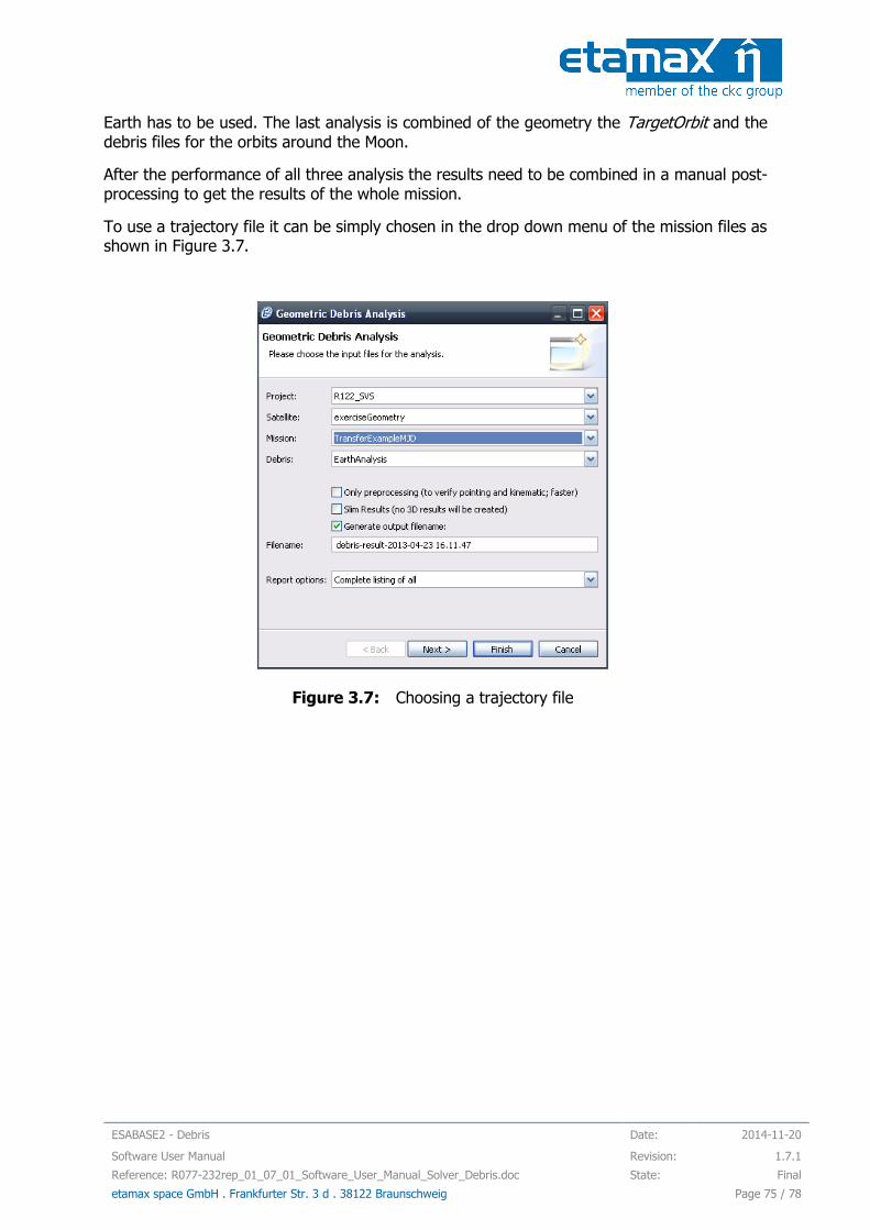
ESABASE2 - Debris Date: 2014-11-20
Software User Manual Revision: 1.7.1
Reference: R077-232rep_01_07_01_Software_User_Manual_Solver_Debris.doc State: Final
etamax space GmbH . Frankfurter Str. 3 d . 38122 Braunschweig Page 75 / 78
Earth has to be used. The last analysis is combined of the geometry the TargetOrbit and the debris files for the orbits around the Moon.
After the performance of all three analysis the results need to be combined in a manual post-processing to get the results of the whole mission.
To use a trajectory file it can be simply chosen in the drop down menu of the mission files as shown in Figure 3.7.
Figure 3.7: Choosing a trajectory file

Date: 2014-11-20 ESABASE2 - Debris
Revision 1.7.1 Software User Manual
State: Final Reference: R077-232rep_01_07_01_Software_User_Manual_Solver_Debris.doc
Page 76 / 78 etamax space GmbH . Frankfurter Str. 3 d . 38122 Braunschweig
4 Additional Information on Specific Debris Analyses
Debris analyses on special orbits can require specific configurations or have specific limita-tions. Such information is listed in the following. The current content of this chapter is:
Specific information for analyses on L1/L2 orbits.
4.1 Specific Information for Analyses on L1/L2 Orbits
This section describes the specifics of configurations and limitations, which should be consid-ered for the analyses of satellites at L1/L2 orbits. The information concerns the analyses using the
Mission file, and
Trajectory file.
4.1.1 L1/L2 Orbits with Mission File
4.1.1.1 L1/L2 Orbit Definition via Mission File
The mission file can be created as described in /1/ section 3.1. The central body “Earth” pro-vides the orbit type options “L1” and “L2”. The Figure 4.1 shows a defined L1 orbit.
Figure 4.1: L1 orbit definition in the mission editor
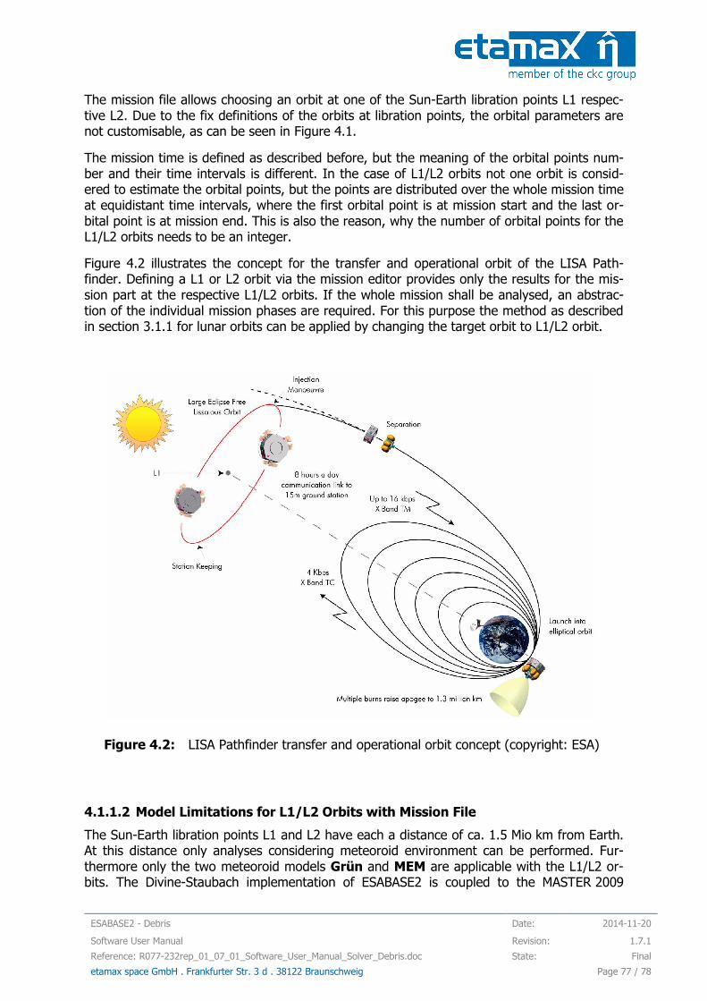
ESABASE2 - Debris Date: 2014-11-20
Software User Manual Revision: 1.7.1
Reference: R077-232rep_01_07_01_Software_User_Manual_Solver_Debris.doc State: Final
etamax space GmbH . Frankfurter Str. 3 d . 38122 Braunschweig Page 77 / 78
The mission file allows choosing an orbit at one of the Sun-Earth libration points L1 respec-tive L2. Due to the fix definitions of the orbits at libration points, the orbital parameters are not customisable, as can be seen in Figure 4.1.
The mission time is defined as described before, but the meaning of the orbital points num-ber and their time intervals is different. In the case of L1/L2 orbits not one orbit is consid-ered to estimate the orbital points, but the points are distributed over the whole mission time at equidistant time intervals, where the first orbital point is at mission start and the last or-bital point is at mission end. This is also the reason, why the number of orbital points for the L1/L2 orbits needs to be an integer.
Figure 4.2 illustrates the concept for the transfer and operational orbit of the LISA Path-finder. Defining a L1 or L2 orbit via the mission editor provides only the results for the mis-sion part at the respective L1/L2 orbits. If the whole mission shall be analysed, an abstrac-tion of the individual mission phases are required. For this purpose the method as described in section 3.1.1 for lunar orbits can be applied by changing the target orbit to L1/L2 orbit.
Figure 4.2: LISA Pathfinder transfer and operational orbit concept (copyright: ESA)
4.1.1.2 Model Limitations for L1/L2 Orbits with Mission File
The Sun-Earth libration points L1 and L2 have each a distance of ca. 1.5 Mio km from Earth. At this distance only analyses considering meteoroid environment can be performed. Fur-thermore only the two meteoroid models Grün and MEM are applicable with the L1/L2 or-bits. The Divine-Staubach implementation of ESABASE2 is coupled to the MASTER 2009
Date: 2014-11-20 ESABASE2 - Debris
Revision 1.7.1 Software User Manual
State: Final Reference: R077-232rep_01_07_01_Software_User_Manual_Solver_Debris.doc
Page 78 / 78 etamax space GmbH . Frankfurter Str. 3 d . 38122 Braunschweig
model and thus only applicable up to a radius 1000 km about GEO radius. The LunarMEM model is a MEM model tailored to the Moon’s vicinity. For this reasons the Divine-Staubach and the LunarMEM models are not applicable with L1/L2 orbits.
4.1.2 L1/L2 Orbit Definition via Trajectory file
The Trajectory file and its use are already described in chapter 3 for the lunar missions. The given characteristic in that chapter are also applicable for the L1/L2 orbits. This means for example that the available environment models are MASTER 2009 and ORDEM 3.0 for Debris and Grün, MEM and LunarMEM for the meteoroids, where LunarMEM is switched to MEM internally.
Beside the descriptions above the following information could be also of interest.
With the L1/L2 orbits analyses capability the “Target”s “L1” and “L2” were introduced, as listed in section 3.1.2. “L1” and “L2” can be used only as targets and “Earth” as origin is mandatory for this cases. Furthermore it is insignificant if you use “L1” or “L2” for the trajec-tory, except for the clarity of the track defined by the trajectory file for the user. The back-ground is the following.
The orbits at the Sun-Earth libration points L1 and L2 are interpreted as Earth bounded or-bits. In this case the configuration would be “Origin: Earth, Target: Earth”. But such configu-ration would lead to an abortion of the execution for a trajectory aiming at a libration point, because Earth’s sphere of influence of hardly 1 Mio km is exceeded and the software is not able to interpret the state vectors any more due to missing central body. To avoid this prob-lem “L1” and “L2” are introduced. Actually both options have the same functionality, they trigger a virtually extension of Earth’s sphere of influence, and are not restricted to the listed state vectors of the file. (So you can use “L2” for state vectors of a L1 orbit and vice versa.)
The method behind is simple. For an Earth bounded path in the trajectory file which exceeds Earth’s usual sphere of influence the “Target” “L1” (or “L2”) is applied. During the parsing of the file HEAD this “L1” (or “L2”) statement is interpreted as a trigger to extend Earth’s sphere of influence to ca. 3 Mio km. After the extension the “Target” is reset to “Earth”. In this way the state vectors in the trajectory file are interpreted as Earth bounded flying path, but the Earth is considered to be the central body for a very high distance.