University of Nebraska - LincolnDigitalCommons@University of Nebraska - LincolnDissertations & Theses in Earth and AtmosphericSciences Earth and Atmospheric Sciences, Department of

2010

EOCENE CALCAREOUS NANNOFOSSILBIOSTRATIGRAPHY, PALEOECOLOGY ANDBIOCHRONOLOGY OF ODP LEG 122 HOLE762C, EASTERN INDIAN OCEAN(EXMOUTH PLATEAU)Jamie L. ShamrockUniversity of Nebraska-Lincoln, jamie.l.shamrock@exxonmobil.com

Follow this and additional works at: http://digitalcommons.unl.edu/geoscidiss

This Article is brought to you for free and open access by the Earth and Atmospheric Sciences, Department of at DigitalCommons@University ofNebraska - Lincoln. It has been accepted for inclusion in Dissertations & Theses in Earth and Atmospheric Sciences by an authorized administrator ofDigitalCommons@University of Nebraska - Lincoln.

Shamrock, Jamie L., "EOCENE CALCAREOUS NANNOFOSSIL BIOSTRATIGRAPHY, PALEOECOLOGY ANDBIOCHRONOLOGY OF ODP LEG 122 HOLE 762C, EASTERN INDIAN OCEAN (EXMOUTH PLATEAU)" (2010).Dissertations & Theses in Earth and Atmospheric Sciences. 42.http://digitalcommons.unl.edu/geoscidiss/42

EOCENE CALCAREOUS NANNOFOSSIL BIOSTRATIGRAPHY, PALEOECOLOGY AND

BIOCHRONOLOGY OF ODP LEG 122 HOLE 762C, EASTERN INDIAN OCEAN

(EXMOUTH PLATEAU)

by

Jamie L. Shamrock

A DISSERTATION

Presented to the Faculty of

The Graduate College at the University of Nebraska

In Partial Fulfillment of Requirements

For the Degree of Doctor of Philosophy

Major: Earth and Atmospheric Sciences (Geology)

Under the supervision of David K. Watkins

Lincoln, Nebraska

November, 2010

EOCENE CALCAREOUS NANNOFOSSIL BIOSTRATIGRAPHY, PALEOECOLOGY AND

BIOCHRONOLOGY OF ODP LEG 122 HOLE 762C, EASTERN INDIAN OCEAN

(EXMOUTH PLATEAU)

Jamie L. Shamrock, Ph.D.

University of Nebraska, 2010

Adviser: David K. Watkins

A relatively complete section of Eocene (~33.9-55.8 Ma) pelagic chalk from offshore

northwestern Australia was used to analyze range and abundance data of ~250 Eocene species to

test the efficacy of the existing CP (Okada and Bukry 1980) and NP (Martini 1971)

biostratigraphic zonation schemes. Changes in nannofossil diversity, abundance, and community

structure were monitored through several Eocene paleoenvironmental events, as identified by

changes in δ13

C and δ18

O data, to examine variations in surface water conditions. Major changes

in nannofossil assemblages, as indicated by dominance crossovers, correspond to

paleoenvironmental shifts such as the Paleocene-Eocene Thermal Maximum and the Early

Eocene Climatic Optimum. This research also provides systematic paleontology and range data

for nine new species and one new genus, and addresses several taxonomic issues in other Eocene

species.

Examination of the calcareous nannofossil biostratigraphy (Section I) showed several

potential hiatuses within the stratigraphic section at Hole 762C. The presence of these hiatuses

was supported by cross-correlation of planktonic foraminiferal P-zones, magnetostratigraphic

reversals and δ13

C and δ18

O isotopic excursions. A portion of the dissertation was conducted to

fulfill the need for a new, integrated age model for Hole 762C, utilizing biostratigraphic,

magnetostratigraphic, and stable isotopic data published in the Leg 122 Initial Reports (Haq et al.

1990) and Scientific Results (von Rad et al. 1992) with the calcareous nannofossil data generated

in Section I. This new age model allowed revision of sedimentation rates at Site 762, and these

revised rates were used to estimate the ages of calcareous nannofossil bioevents, which are

compared to several additional, globally distributed localities.

iv

ACKNOWLEDGEMENTS

This research used samples and data provided by the Deep Sea Drilling Program (DSDP)

and Ocean Drilling Program (ODP). The DSDP and ODP are sponsored by the National Science

Foundation (NSF) and participating countries under the management of Joint Oceanographic

Institutions (JOI) Inc. The author would like to thank David K. Watkins, Mary Anne Holmes,

Tracy Frank (University of Nebraska-Lincoln, Earth & Atmospheric Sciences) and Paul Hanson

(UN-L, School of Natural Resources) and Kurt Johnston (ExxonMobil) for their role as doctoral

committee members and for their collaboration and revisions on this dissertation. The author

would also like to thank Jackie Lees and Tom Dunkley-Jones (Imperial College London) for

their revisions on the manuscript published in the Journal of Nannoplankton Research (Section

II).

v

TABLE OF CONTENTS

Dissertation Introduction 1

Section I - Eocene calcareous nannofossil biostratigraphy and community structure

from Exmouth Plateau, Eastern Indian Ocean 3

Chapter 1 - Introduction 3

Chapter 2 - Materials and Methods 5

Chapter 3 - Results 7

3.1 - Calcareous Nannofossil Biostratigraphy 7

3.2 - Nannofossil Abundance Trends and Paleoenvironmental Events 19

3.3 - Problem Taxa 33

3.4 - Summary 34

Chapter 4 - Systematic Paleontology 35

Chapter 5 - Conclusions 35

Section II - A new calcareous nannofossil species of the genus Sphenolithus from

the Middle Eocene (Lutetian) and its biostratigraphic significance 39

Chapter 1 - Introduction 39

Chapter 2 - Materials and Methods 39

Chapter 3 - Sphenolith Abundance and Distribution 40

Chapter 4 - Sphenolith Morphology and Lineage 41

Chapter 5 - Sphenolith Biostratigraphic Significance 42

Chapter 6 - Sphenolithus perpendicularis n.sp. Systematic Paleontology 43

Section III - Eocene bio-geochronology of ODP Leg 122 Hole 762C, Exmouth Plateau

(northwest Australian Shelf) 46

Chapter 1 - Introduction 46

vi

Chapter 2 - Setting and Stratigraphic Context 48

2.1 - ODP Leg 122 Hole 762C 48

2.2 - Additional Sites 49

Chapter 3 - Data and Methods 51

3.1 - Magnetostratigraphy 51

3.2 - Nannofossil Biostratigraphy 52

3.3 - Planktonic Foraminifera Biostratigraphy 53

3.4 - Isotope Stratigraphy 53

Chapter 4 - Results 56

4.1 - Revised Magnetostratigraphy 56

4.2 - Age-Depth Plot 60

4.3 - Sedimentation Rates and Nannofossil Calibration 61

Chapter 5 - Discussion 65

Chapter 6 - Conclusions 68

LIST OF MULTIMEDIA OBJECTS

Figures:

Figure 1 - Site Map 69

Figure 2 - Nannofossil Biostratigraphy 70

Figure 3 - Isotopic Data and Nannofossil Assemblage Trends 71

Figure 4 - Nannofossil Species Abundance Trends 72

Figure 5 - Nannofossil Genera Abundance Trends 73

Figure 6 - Warm Taxa, Cool Taxa and Holococcolith Abundance Trends 74

Figure 7 - EECO Nannofossil Assemblage Turnovers 75

Figure 8 - Markalius spp. Analysis 76

Figure 9 - Hexadelus and Braarudosphaera Morphological Geometries 77

Figure 10 - Hexadelus and Braarudosphaeraceae Distribution Curves 77

vii

Figure 11 - Sphenolithus perpendicularis n.sp. Abundance Trends 78

Figure 12 - Observed Sphenolithus Ranges 78

Figure 13 - Sphenolith Morphology 79

Figure 14 - Sphenolith Extinction Patterns 79

Figure 15 - Proposed Sphenolithus Lineage 80

Figure 16 - Stratigraphic Data Correlation at Hole 762C 81

Figure 17 - Revised Age-Depth Model 83

Tables:

Table 1 - Lithologic Summary 84

Table 2 - Nannofossil Sample List 85

Table 3 - Nannofossil Biostratigraphy 86

Table 4 - Additional Nannofossil Bioevents 87

Table 5 - Stable Isotopic Data 88

Table 6 - PETM Nannofossil Trends 89

Table 7 - Paleoecological Groupings 90

Table 8 - Sphenolithus Range Data 90

Table 9 - Nannofossil Tie-Points 91

Table 10 - Isotopic Tie-Points 92

Table 11 - Magnetostratigraphy Tie-Points 92

Table 12 - Nannofossil Event Ages 93

Table 13 - Summary of Unconformities 94

Specimen Photo Plates:

Plate 1 - Chiastozygaceae, Calciosoleniaceae, Rhabdosphaeraceae, Zygodiscaceae,

Calcidiscaceae 97

Plate 2 - Calcidiscaceae 98

viii

Plate 3 - Calcidiscaceae, Coccolithaceae 99

Plate 4 - Coccolithaceae 100

Plate 5 - Noelaerhabdaceae, Prinsiaceae 101

Plate 6 - Prinsiaceae, Placolith genera incertae sedis 102

Plate 7 - Placolith genera incertae sedis, Calyptrosphaeraceae 103

Plate 8 - Calyptrosphaeraceae, Lapideacassaceae, Discoasteraceae, Sphenolithaceae,

Nannoliths incertae sedis 104

Plate 9 - Sphenolithaceae, Nannoliths incertae sedis, Indeterminant nannoliths 105

Plate 10 - Sphenolithaceae 106

Appendices:

Appendix A - Nannofossil Systematic Paleontology and Taxonomic Appendix 107

Appendix B - Planktonic Foraminifera Taxonomic Appendix 140

1

DISSERTATION INTRODUCTION

The following dissertation was presented to the faculty of the Graduate College at the University

of Nebraska as partial fulfillment of requirements for the Degree of Doctor of Philosophy, majoring in the

Department of Earth & Atmospheric Sciences. This research is a micropaleontological study of

calcareous nannoplankton from the Eocene epoch (~33.9-55.8 Ma), examining the biostratigraphy,

paleoecology, and geochronology from Ocean Drilling Program (ODP) Leg 122 Hole 762C in the eastern

Indian Ocean (northwest Australian continental shelf; Figure 1).

The dissertation is divided into three sections. As partial fulfillment of PhD requirements in the

Department of Earth & Atmospheric Sciences, research projects should be of sufficient scope and

complexity to produce a minimum of three research papers suitable for publication in scientific journals.

Each of the following sections represents one such prospective publication.

Section I

This section of the dissertation was conducted to fulfill a need for a continuous Eocene calcareous

nannofossil reference section, using samples from Leg 122 Hole 762C. A primary goal was to collect and

analyze range and abundance data for a vast number of Eocene species, relative to the preexisting CP

(Okada and Bukry 1980) and NP (Martini 1971) biostratigraphic zonation schemes. This data is used to

examine the changes in nannofossil diversity, abundance, and community structure through several

Eocene paleoenvironmetnal events, as identified by changes in δ13C and δ18O data. This research also

provides systematic paleontology and range data for eight new species and one new genus, and addresses

several taxonomic issues in other Eocene species (Appendix A).

Section II

This section is a taxonomic study describing a new species, Sphenolithus perpendicularis n.sp,

from the middle Eocene (Lutetian). The distinct morphology and short stratigraphic range of this species,

2

and sister species in this Sphenolithus lineage, indicate good potential for biostratigraphic utility. This

may be particularly true in this biostratigraphic interval (CP13 of Okada and Bukry 1980), where primary

biomarkers may be rare. This portion of the dissertation has been published in 2010 in the Journal of

Nannoplankton Research (volume 31, no. 1).

Section III

The final section of this dissertation was conducted in response to data and results generated in

Section I. Ideally, that research would utilize a relatively complete and expanded succession of strata with

good nannofossil abundance and preservation that could function as a reference section. Arguably the best

existing section for such a purpose was cored by Ocean Drilling Program Leg 122 off of northwest

Australia in 1990, as indicated by data from that expedition (Golovchenko et al. 1992; Haq et al. 1992;

Siesser & Bralower 1992). Reexamination of the calcareous nannofossil biostratigraphy (Section I)

showed several potential hiatuses within the stratigraphic section at Hole 762C. The presence of these

hiatuses was supported by cross-correlation of planktonic foraminiferal P-zones, magnetostratigraphic

reversals and δ13C and δ18O isotopic excursions. This section of the dissertation was conducted to fulfill

the need for a new, integrated age model for Hole 762C, utilizing biostratigraphic, magnetostratigraphic,

and isotopic data published in the Leg 122 Initial Reports (Haq et al. 1990) and Scientific Results (von

Rad et al. 1992) with the calcareous nannofossil data generated in Section I. This new age model allowed

revision of sedimentation rates at Site 762, and these revised rates were used to estimate the ages of

calcareous nannofossil bioevents, which are compared to several additional, globally distributed localities.

3

Section I - Eocene calcareous nannofossil biostratigraphy and community structure from

Exmouth Plateau, Eastern Indian Ocean

Chapter 1 - INTRODUCTION

The Eocene Epoch is a critical transition period from the global greenhouse conditions of the Late

Cretaceous and early Paleogene to the icehouse of the later Cenozoic. The lower boundary is marked by a

distinct pulse of global warmth, the PETM (Paleocene-Eocene thermal maximum), and the upper

boundary by cooling associated with the onset of Antarctic glaciation, with a significant proportion of

research focused on the conditions governing its lower and upper boundaries with the Paleocene and

Oligocene, respectively.

The recent advances in our knowledge of calcareous nannofossils (Bown and Pearson 2009;

Dunkley-Jones et al. 2008; Agnini et al. 2006; Bown 2005; Raffi, Backman and Pälike 2005; Tremolada

and Bralower 2004, others) provide an opportunity to reevaluate the Eocene biostratigraphic succession

and the nannofossil assemblage through significant paleoenvironmetnal changes. This research was

conducted to fulfill a need for a continuous Eocene calcareous nannofossil reference section, containing

range and abundance data for a vast number of Eocene species, relative to the preexisting CP and NP

biostratigraphic zonation schemes. In addition we examine the changes in nannofossil diversity,

abundance, and community structure through several Eocene paleoenvironmetnal events. Ideally, this

study would utilize a relatively complete succession of strata that could function as a reference section.

Arguably the best existing section for such a purpose was cored by Ocean Drilling Program Leg 122 at

Hole 762C off of northwest Australia in 1990. The thorough biostratigraphic characterization of Siesser

& Bralower (1992) demonstrated a relatively complete and expanded Eocene succession with good

nannofossil abundance and preservation. In addition, there are well-documented paleomagnetic (Galbrun

1992) and stable isotopic (Thomas Shackleton and Hall 1992) data for this site.

4

Several recent studies have been conducted on Eocene calcareous nannofossil biostratigraphy

and/or paleoenvironmetnal assemblage trends, producing a wealth of new nannofossil data; however,

many of these studies focus on high resolution analysis of a discrete event, such as the PETM (Paleocene-

Eocene thermal maximum) (Bown and Pearson 2009; Raffi, Backman and Pälike 2005; Tremolada and

Bralower 2004), MECO (middle Eocene climatic optimum) (Jovane et al 2007), and Oi-1 events

(Dunkley-Jones et al. 2008), or such research is restricted to only a portion of the epoch (Villa et al. 2008;

Agnini et al. 2006). There are few studies where the nannofossil assemblage and range data has been

quantitatively examined throughout the entire Eocene, particularly from one locality.

Recent research from the Southern Ocean (Persico and Villa 2008) and Tanzania (Bown

Dunkley-Jones and Young 2007; Bown and Dunkley-Jones 2006; Bown 2005) has named a significant

number of new calcareous nannofossil species. This research confirms the presence of 41 of these species

within the eastern Indian Ocean at Site 762, and expands the ranges of several of these taxa. In addition,

we provide systematic paleontology and range data for eight additional new species and one new genus,

and address taxonomic issues with several additional forms.

In addition to developments in nannofossil biostratigraphy, the construction of high-resolution

δ13C and δ18O records (Galeotti et al. 2010; Bohaty et al. 2009; Nicolo et al. 2007; Lourens et al. 2005;

Bohaty and Zachos 2003; Zachos et al. 2001; others) has allowed paleoenvironmental events such as the

PETM, ETM2 (Eocene thermal maximum 2), ETM3, EECO (early Eocene climatic optimum), MECO

and Oi-1 to be identified at Site 762. Lower resolution δ13C and δ18O reocords for Site 762 of Thomas

Shackleton and Hall (1992) allows identification of many key excursions throughout the Eocene, which

allows us to examine the dynamics of the nannofossil community with respect to such

paleoenvironmental events. We identify significant assemblage turnovers in the middle Eocene and

discuss the possible relationships of these data to both short term environmental perturbations and the

long term climate transition from global greenhouse to icehouse.

5

Chapter 2 - MATERIALS AND METHODS

ODP (Ocean Drilling Program) Leg 122 Hole 762C was selected for this study because of a thick,

expanded Eocene succession (~240 m) as well as data from Leg 122 Initial Reports (Haq et al. 1990) and

Scientific Results (von Rad et al. 1992) that indicate relatively continuous sedimentation. Site 762

(19°53.23S, 112°15.24E) is located on the central Exmouth Plateau (northern Carnavon Basin) (Figure 1)

and is separated from the Australian Northwest Shelf by the Kangaroo Syncline (von Rad et al. 1992).

Though stretched and rifted in its early history, the plateau has been relatively quiescent since the mid-

Cretaceous, with fairly uniform thermal subsidence. Hole 762C was drilled in 1360m of water, with

decompacted burial curves indicating little change in water depth since the time of original deposition

(Haq et al. 1992).

Approximately 240 m of Eocene sediments were penetrated in Cores 3-29 from ~184-422 msbf

(meters below sea floor). Core recovery varies throughout this interval, ranging from 12.1 to ≥ 100%,

with an average recovery of ~67% (Figure 2). Sedimentation rate estimates are ~1-3 cm/ky in the early

Eocene and ~0.5-2 cm/ky in the mid- and late Eocene (Shipboard Scientific Party 1990; Haq et al. 1992).

Eocene pelagic sediments from this locality consist of white to green-grey, calcareous oozes, chalks, and

marls, indicating an open-ocean setting (von Rad et al. 1992). Clay content and bioturbation increased

downward toward the lower Eocene. This interval is divided into three lithologic subunits as described in

Haq et al. (1992) and is summarized in Table 1. Calcareous nannofossil data from Siesser & Bralower

(1992) show a diverse and robust nannofossil assemblage, and biostratigraphy based on the NP zonation

(Martini 1971) suggests a relatively complete Eocene succession. Calcareous nannofossils are extremely

abundant and moderately to well preserved, with deposition well above the CCD (carbonate

compensation depth).

A total of 187 samples were selected from the recovered core at approximately 0.75 m intervals,

as core availability would allow. Of these samples, 102 were used to collect detailed assemblage data,

6

with the remaining samples used to increase precision of key biostratigraphic markers. Sample intervals

and depths are provided in Table 2. All samples span a 1 cm interval (downward), excluding 14-3-125 (2

cm) and 13-2-71, 15-2-52, and 21-5-50.5 (1.5 cm). Though some samples occur on half-centimeter

intervals, depths have been rounded to two significant digits. Due to significant expansion of Core 26

(182% recovery), samples from this core required calibration of true depths (in mbsf) by taking the cored

interval by the total thickness (4.5 m/7.8 m recovered thickness) to get a ratio (0.616 m true depth/ 1 m

recovered thickness). This ratio was applied to samples from Core 26 to generate depths (Table 2).

Sample midpoints in Table 3 represent the midpoint of the error between the observed event depth and the

sample below (for LOs; lowest occurrence) or the sample above (for HOs; highest occurrence).

Core samples and smear slides, including holotype and paratype materials and photographs, are

housed within the collections of the ODP Micropaleontological Reference Center at the University of

Nebraska State Museum (UNSM). Smear slide preparation for Hole 762C followed standard techniques

as described by Bown and Young (1998) and were mounted using Castolite AP Crystal Clear Polyester

Resin. Smear slides were examined at 1000-1250x magnification with an Olympus BX51 and a Zeiss

AxioImager A.2 under plane parallel light (PL), cross-polarized light (XPL), and with a one-quarter λ

mica interference plate.

Assemblage data was collected by first identifying 500 specimens to species level, except

members of Pontosphaeraceae and Syracosphaeraceae, which were rare and sporadic through the section

(See appendix A). Additionally, two long traverses were examined to identify rare specimens, which were

given a value of 1 and added to the total. These data were used to convert all species and genera to

percent abundance for further analysis.

Counts of 300 specimens are considered statistically significant (Revets 2004; Dennison and Hay

1967; Phleger 1960) for identifying species that account for ~ 0.01% of the nannofossil assemblage with

p = 0.05 (95% confidence interval); however, by generating counts > 456 specimens for percent

abundance data, at the 95% confidence interval, the maximum second standard deviation will be ≤ 5% of

7

the actual proportion (Chang 1967). Diversity and univariate statistical analysis was conducted on the

data using PAST (Paleontological Statistics) software (Hammer et al., 2001).

Chapter 3 - RESULTS

Approximately 260 taxa were identified through this Eocene section, including 41 recently named

and 8 new species, with nearly all CP and NP zones and subzones identified at Site 762. Calcareous

nannofossils were abundant, with >10 – 100 specimens per FOV (field of view). Nannofossil specimens

were moderately to well-preserved, with little or some etching, recrystallization, and alteration of primary

morphology . Reworked Cretaceous and Paleogene specimens were very rare. Ranges are provided for

all species as well as notable abundance trends and taxonomic issues (See appendix).

Several families are believed to inhabit neritic/shelf environments due to their general paucity in

open-ocean settings, such as Syracosphaeraceae (Seisser 1998; Roth and Berger 1975),

Rhabdosphaeraceae (Perch-Nielsen 1985; Roth and Thierstein 1972), Pontosphaeraceae (Perch-Nielsen

1985), Braarudosphaeraceae (Bybell and Gartner 1972; Sullivan 1965), and most holococcoliths

(Gartner, 1969). The nannofossil assemblage at Hole 762C is consistent with an open ocean setting, as all

such taxa were rare, sporadic, and/or absent from this locality. Despite the relative absence of some

families, the nannofossil assemblage shows high species richness (S) throughout the Eocene (µ = 53.4,

Max. = 66, Min. = 41). Additional data and results are incorporated into the biostratigraphy and

paleoenvironmental discussions, below.

3.1 - Calcareous Nannofossil Biostratigraphy

Two well known and widely employed biozonation schemes are generally applied in Paleogene

calcareous nannofossil biostratigraphy: the low-latitude Okada-Bukry (1980) CP Zonation and the

cosmopolitan to high-latitude Martini (1971) NP Zonation. Calcareous nannofossil biostratigraphy for

8

ODP Leg 122 Site 762C was originally examined by Siesser and Bralower (1992) using a modified

version of the NP zonation, that incorporated CP markers, and other alternative markers, where the range

and abundance of NP markers were in question. This locality has been reexamined using both the

standard CP and NP zonations, with select NP subzones of Aubry (1991), to compare the consistency of

these two zonation schemes, as well as to examine the secondary and alternative markers frequently

employed. Strict application of some zones was not possible, due to the rarity or absence of some marker

taxa at Hole 762C (R. gladius, D. bifax, N. alata). Subzones in the NP zonation scheme were not

originally applied in Siesser and Bralower (1992) but have been identified based on data from that study.

Sample intervals and depths of key marker taxa are provided in Table 3. Figure 2 illustrates the CP and

NP nannofossil biostratigraphy at Hole 762C from the current study, as well as from Siesser and Bralower

(1992). Placement of boundaries between the Eocene stages is tentative, as no nannofossil bioevents

directly mark these horizons (Ogg Ogg and Gradstein 2008). Stage boundaries were approximated using

nannofossil events in conjunction with dated isotopic excursions, identified from original ODP Leg 122

δ13C and δ18O data of Thomas, Shackleton and Hall (1992) (See “Nannofossil Abundance Trends”,

below).

The original interpretation of Siesser and Bralower (1992) identified all NP zones with no

apparent hiatuses; however, this study identifies zones and subzones that are absent from both the NP and

CP zonation schemes. The NP zonal boundaries are essentially congruent between Siesser and Bralower

(1992) and this study for NP9, NP11, NP12, NP13, NP15, NP19/20, and NP21. Minor differences are

due to core recovery issues, sample spacing between studies, or perhaps time with each sample: Many key

taxa were very rare at Site 762, and significant time was spent searching for rare marker taxa,

subsequently shifting the zonal boundaries. Significant differences do exist at the NP10, NP14, NP16,

NP17, and NP18 boundaries, related to either use of CP and/or alternative markers or from a stratigraphic

hiatus, and are discussed in greater detail below. Nannofossil zones are discussed with respect to the basal

biomarker, with the top defined by the base of the following zone.

9

The variations in the NP and CP interpretations, both within our data and in comparison to earlier

work, show some issues that can arise with rare, diachronous, and/or secondary taxa. When possible it

may be best practice to employ both zonation schemes, as comparison of the two interpretations may shed

light on hiatuses and/or marker taxa that occur too high or too low in the section. An increase in

latitudinal temperature gradients, as seen in the late Eocene, tends to increase both the degree of

taxonomic provinciality and the severity of diachronism for many paleontological proxies. This decreases

the resolution of the biostratigraphic record during dynamic transitions when it is most needed, and gives

further support to the application of a robust and diverse set of biomarkers whose stratigraphic

relationships to one another are well understood.

Zones CP8a/NP9

The basal sample in this study (29-1-50 cm, 422.00 msbf) contains Discoaster multiradiatus, the

marker taxa for the base of CP8/NP9. Siesser and Bralower sampled significantly deeper through the

section and their midpoint for the LO of D. multiradiatus also occurs at 422.00 msbf, so our section

begins near the base of this zone.

Subzone CP8b is absent from Hole 762C. Both the primary marker (LO Campylosphaera eodela)

and the secondary marker (LO Rhomboaster spp.) are concurrent with the LO of D. diastypus, which

marks the base of subzone CP9a (28-1-59 cm, 412.59 mbsf). This convergence is most noticeable using

CP subzonal markers, and may not be identified with the NP scheme (Figure 2). This hiatus occurs in

association with the PETM (412.65 msbf), and corresponds to a notable change in the nannofossil

assemblage, treated more thoroughly in the PETM discussion below.

Zones CP9a/NP10

The base of CP9a (LO Discoaster diastypus) may be slightly younger than the base of NP10 (LO

Tribrachiatus (Rhomboaster) bramlettei) (Ogg Ogg and Gradstein 2008); however, these bioevents were

10

observed in the same sample (28-1-59 cm, 412.59 mbsf). The LO of D. diastypus may serve as a proxy

for the NP marker in sections where members of Rhomboasteraceae are rare. The secondary marker of

Perch-Nielsen (1985), the HO of Fasciculithus spp., was also observed in this sample. Though these three

bioevents are in good agreement at Hole 762C, this convergence may be due to the underlying hiatus and

truncation of the true event depths.

The base of NP10 in Siesser and Bralower (1992) was marked by the LO of T. contortus (27-3-99

cm, 406.49 mbsf), as it was observed before the primary marker (LO T. bramlettei) (27-1-99 cm, 403.49

mbsf) in that study. We observed the LO of T. bramlettei significantly below this depth (28-1-59, 412.59

mbsf). This discrepancy is likely a reflection of the general rarity of these forms at Site 762 and that

relationship to probability of identification (see above). Raffi, Backman and Pälike (2005) also note that

rarity and identification issues with intermediate forms may hinder use of the Tribrachiatus lineage.

Agnini et al. (2007a) also questions the reliability of T. bramlettei as a primary marker taxa, suggesting

that observed diachroniety may be a true environmental signal, or may be a preservational issue, related to

dissolution of basal Eocene deposits in conjunction with the PETM.

Zones CP9b/NP11

The bases of both CP9b and NP11 are marked by HO of Tribrachiatus contortus (26-1-49 cm,

398.30 mbsf). The secondary marker of Perch-Nielsen (1985), the LO of T. orthostylus, is not concurrent

in Hole 762C, but occurs immediately above (25-5-43 cm, 394.93 mbsf). This secondary marker taxa may

be more readily applied, as T. orthostylus is often more abundant that T. contortus.

Agnini et al. (2007a) have proposed the LO of Sphenolithus radians as an alternate biomarker for

the base of NP11/CP9b. The LO of S. radians was observed in the same sample as the LO of T.

orthostylus at Site 762 (Indian Ocean), and agrees with data from the southeast Atlantic (Agnini et al.

2007a), equatorial Pacific (Raffi, Backman and Pälike 2005) and western Tethys (Agnini et al. 2006).

11

Zones CP10/NP12

The LO of Discoaster lodoensis (23-3-51 cm, 373.01 mbsf) marks the base of both CP10 and

NP12. One of the secondary bioevents for CP10, the LO D. kuepperi (Perch-Nielsen 1985), was

concurrent with D. lodoensis and significantly more abundant at the base of its range that the primary

marker, suggesting high potential as a proxy event. The second alternate marker of Perch-Nielsen (1985)

(LO Rhabdosphaera truncata) was observed below D. lodoensis (24-1-54 cm, 379.54 mbsf) and was

relatively rare and sporadic through its range.

Zones CP11/NP13

These zones mark the first real taxonomic divergence of the two biozonation schemes, resulting

in quite different interpretations of Hole 762C depending upon which scheme is employed. The base of

CP11 is marked by the LO of Coccolithus crassus (20-1-50 cm, 341.50 mbsf). NP13 is marked by the HO

of Tribrachiatus orthostylus (also the 2° marker for CP11 (Perch-Nielsen, 1985)); however, there is no

apparent separation between this event and the base of NP14a (LO D. sublodoensis) at Hole 762C. In

fact, extrapolation upward and downward for the HO and LO, respectively, creates a depth crossover as

shown in Table 3

Co-occurence of T. orthostylus and D. sublodoensis (19-2-52 cm, 333.52 mbsf) indicates NP13 is

absent from Site 762. The presence of CP11 without NP13 is possible in several ways: The HO of T.

orthostylus may occur too high in the section (the HO of T. orthostylus is noted as unreliable by Wei and

Wise (1989b), occurring between 51-54.8 Ma in the south Atlantic and Pacific Oceans). Discoaster

sublodoensis may show an early first occurrence, reducing the thickness of CP11 and compressing or

eliminating NP13 (See below). Additionally, there may be a hiatus that removed NP13 and the upper

portion of CP11, leaving only the basal portion of CP11 in the biostratigraphic record. This issue may not

have been recognized if only the CP zonation scheme was applied, but is quite obvious in the NP scheme,

or when the two are used together.

12

Zones CP12a/NP14(a)

Both CP and NP zones are marked by the LO of Discoaster sublodoensis. As mentioned above,

D. sublodoensis may occur too low in the section, and we observe the LO of D. sublodoensis even deeper

(from CP10, 20-3-52, 344.52 msbf) than the LCO (19-1-125, 332.75 m) used here to mark the base of

these zones. A similar distribution is also observed by Agnini et al. (2006), Mita (2001), Wei and Wise

(1990a), and Monechi and Thierstein (1985) in CP10 and CP11, prior to the LCO and base of CP12a.

Only specimens with five straight, pointed rays were identified as D. sublodoensis, so it is unlikely that

these early forms are misidentified specimens of D. lodoensis. Siesser and Bralower (1992) identified

this bioevent slightly higher in the section (330.50 msbf) resulting in a modest NP13 in the original

interpretation. It is possible that D. sublodoensis shows an early LO at Exmouth Plateau, reducing the

thickness of both CP11 and NP13.

Zones CP12b/NP14(b)

The LO of Rhabdosphaera inflata (17-5-148 cm, 319.98 mbsf) marks the base of both CP12b and

NP14b. Though relatively rare, this species is consistently present through its range.

Zones CP13(a-b)/NP15(a-c?)

The base of CP13(a) and NP15 is marked by the LO Nannotetrina fulgens (16-4-45 cm, 307.95

mbsf). The secondary marker of Perch-Nielsen (1985) for the base of CP13a, the HO of Rhabdosphaera

inflata (17-1-51 cm, 313.01 mbsf) occurs in the sample immediately below the LO of N. fulgens, and

extrapolation of midpoints makes these events nearly isochronous. CP13 is subdivided into CP13b and

CP13c by the LO and HO of Chiasmolithus gigas, respectively, and these subzonal markers are often

similarly applied to NP15. The HO of Ch. gigas and the LO of Reticulofenestra umbilica were observed

in the same sample (292.00 msbf), suggesting a hiatus through this subzone. A very thin interval can be

attributed to NP15c (Table 3), as the NP and CP schemes use different taxa for the boundaries above;

however, this thin (~0.75 m) interval may be an artifact of sample spacing or rarity of marker taxa.

13

Zones CP14a/NP16

The base of CP14a is marked by the LO of R. umbilica, while the base of NP16 is marked by the

HO(s) of Blackites gladius and/or Nannotetrina fulgens. The 1° zonal marker, Blackites gladius, was not

observed in this section, so this zone has been identified by the HO N. fulgens, though the genus as a

whole is notably rare at this locality. The LO of R. umbilica (14-6-50; 292.00 mbsf), the HO of N. fulgens

(14-5-115 cm, 291.15 mbsf) and the HO of Ch. gigas (14-6-50 cm, 292.00 mbsf) show very little

stratigraphic separation in Hole 762C, indicating a hiatus comprising all of CP13c and at least a

significant portion of NP15c.

There appears to be a significant difference in the location of the NP16 boundary between this

study and Siesser and Bralower (1992) (Table 3), who use the HO of Nannotetrina spp. to identify the

base of NP16; however, the HO of N. fulgens and the HO of Nannotetrina spp. are nearly congruent

between studies (2.35 and 0.95 m separation, respectively), and strict application of the NP zonation

scheme resolves this apparent offset. The HO of Nannotetrina spp. may be observed higher in the section

than the HO of N. fulgens, which highlights the biostratigraphic issues that occur with rare taxa, where

nannofossil workers are often required to use alternative markers that may or may not be well correlated.

Zones CP14b/NP17

The HO Chiasmolithus solitus (12-3-125 cm, 269.25 mbsf) marks the base of both CP14b and

NP17. This species was rare at Site 762 and was often not identified until > 3 traverses. Siesser and

Bralower (1992) identify the HO of Ch. solitus significantly lower in the section (13CC, 284.00 mbsf),

and do not use the HO of this species to mark the NP17 boundary, due to its rarity. Differences in the

apparent range are likely related to the number of FOVs (field of view) and probability of finding rare

taxa. This results in low confidence when picking the CP14b/NP17 boundary, particularly at mid- to low-

latitude sites where Chiasmolithus spp. may be rare (Villa et al. 2008, Tremolada and Bralower 2004).

Siesser and Bralower (1992) instead use two events as a proxy for the NP17 boundary: the LOs of

14

Cribrocentrum (Reticulofenestra) reticulatum and Helicosphaera compacta, which they identify at 12-6-

100 cm (273.50 mbsf) and 12-5-100 cm (272.00 mbsf), respectively. The authors’ events are reasonably

near our observed HO of Ch. solitus (269.25 msbf); however, these bioevents are placed in CP14a in this

study.

Tremolada and Bralower (2004) suggest that the HO of Ch. solitus is time transgressive over

varying paleolatitudes: common at high latitudes until extinction, but rare and sporadic at lower latitudes

prior to the HO, so that the event becomes older as latitude decreases. The predominantly mid- to low-

latitude assemblage identified at Site 762 suggests that such rarity and/or diachroniety may affect the HO

of this biostratigraphic marker.

These issues highlight the need for a reliable alternative bioevent. The HO of Discoaster bifax

has also been used to mark the base of CP14b, but, similar to Ch. solitus, D. bifax can be extremely rare,

and few specimens were identified in Hole 762C. In addition, Wei and Wise (1989a) suggest that the

morphological transition between D. praebifax and D. bifax may hinder its use. Alternatively, the FCO of

R. hillae and the LO of Dictyococcites (Reticulofenestra) bisectus (< 10 μm) were both observed in

sample 12-4-50 cm (270.0 mbsf), and closely approximate the HO of Ch. solitus (12-3-125, 269.25m).

Bown (2005) and Marino and Flores (2002) also identify the LO of D. bisectus just above the HO of Ch.

solitus, suggesting potential for this species as an alternate marker for CP14b/NP17.

Zones CP15a/NP18

The base of CP15a is marked by the HO Chiasmolithus grandis (10-1-50 cm, 246.5 mbsf), while

the base of NP18 is marked by the LO Ch. oamaruensis (8-5-50 cm, 233.5 mbsf). These events are shown

as nearly contemporaneous in the 2008 Time Scale (Ogg Ogg and Gradstein 2008). The stratigraphic

separation between these bioevents in Hole 762C may be artificially expanded by poor recovery of Core

9x (Figure 2). In addition, Ch. grandis and Ch. oamaruensis are quite rare near their HO and LO,

respectively, and were often only identified after >3 traverses across a slide. Use of sample mid-points

15

greatly reduces this separation, but still results in stratigraphic offset and uncertainty in placement of

zonal boundaries (Figure 2). Though some specimens of Ch. oamaruensis are readily identified, the

narrow angle between cross-bars that defines this species can be difficult to distinguish from similar taxa

such as Ch. altus and Ch. eoaltus, which have a larger angle between cross-bars. This uncertainty,

combined with rarity, can create difficulties when applying this marker.

Zones CP15b/NP19/20

The LO of Isthmolithus recurvus marks the base of both CP15b and NP19/20. The FCO is used

to mark the base of the (sub)zone at Site 762 (7-1-50 cm, 218.0 mbsf), as two isolated specimens were

observed deeper in the section (236.96 and 223.46 msbf). Villa, et al. (2008) identify rare occurrences of

I. recurvus in CP15a, and also use the FCO to mark the base of the subzone.

The secondary CP marker of Perch-Nielsen (1985), the HO of Cribrocentrum (Reticulofenestra)

reticulatum (4-1-123.5 cm, 190.24 mbsf), was observed significantly above the FCO of I. recurvus. This

stratigraphic relationship is also shown by Cascella and Dinarés-Turell (2009), Villa et al. (2008), Marino

and Flores (2002a, b), Berggren et al. (1995), and Wei and Wise (1989b). Calibration of the HO of Cr.

reticulatum by Berggren et al (1995) dates the HO of this species approximately 1 My earlier at high

latitudes than at low latitudes.

Zones CP16a/NP21

The CP16a and NP21 boundaries are marked by the HO of D. saipanensis (and/or the HO D.

barbadiensis). The HO of D. saipanensis (and D. barbadiensis) has been problematic at Site 762. Very

rare and sporadic specimens of both species were observed quite high in the section, through the highest

sample in this study (3-1-49 cm; 184.49 mbsf) and through sample 2-2-100 cm (172.5 mbsf) in the

original interpretation. This difficulty in boundary placement due to rarity has also been noted by

Dunkley-Jones and others (2008) and Siesser and Bralower (1992). Rare but consistent specimens of D.

saipanensis and D. barbadiensis were observed through 4-3-100 cm (193.0 mbsf), marking the HCO of

16

both species, and the base of CP16a in this study. The upper two samples in this study are located within

CP16a, as both contain Reticulofenestra oamaruensis and show a considerable increase in Clausicoccus

spp., marking the base of this acme event.

Synthesis

Application of both the Okada and Bukry (1980) CP zonation and the Martini (1971) NP zonation

facilitated the identification of three stratigraphic hiatuses. Hiatus A was identified with the CP zonation,

by the concurrent LOs of Campylosphaera eodela, Rhomboaster spp., and Discoaster diastypus (412. 59

msbf) and indicates the absence of subzone CP8b. Hiatus B was identified with the NP zonation, by the

convergence of the HO of Tribrachiatus orthostylus and the LO of D. sublodoensis (333.52 msbf), and

indicates the absence of NP13. Hiatus C was identified in both the CP and NP zonation, as both the LO of

Reticulofenestra umbilica and Nannotetrina fulgens converge with the HO of Chiasmolithus gigas, with

the absence of subzone CP13c/NP15c. While hiatus C can be identified with either zonation scheme, both

the NP and CP zonation are insufficient to readily identify all three hiatuses. These schemes become more

robust when used in conjunction, due to the greater number of nannofossil markers. This allows both

greater biostratigraphic resolution when events are offset (LO R. umbilica/CP14a and N. fulgens/NP16),

and greater confidence when two bioevents are nearly isochronous (HO Ch. gigas/CP15a and LO Ch.

oamaruensis/NP18).

The standard CP and NP nannofossil zonation schemes provided a series of bioevents that are

extremely useful in biostratigraphy, most of which are consistent, reliable, and well-calibrated; however,

some of these taxa are shown to be inconsistent in this research and in several other studies, such as

Discoaster sublodoensis, Chiasmolithus oamaruensis, Ch. solitus, and Tribrachiatus bramlettei. This is

well illustrated when comparing the Site 762 nannofossil biostratigraphy of Siesser and Bralower (1992)

to this reexamination, as all significant divergences in interpretations are linked to these problem taxa.

17

The placement of some zonal boundaries is compromised simply by the rarity of the biomarker

that defines it. Such rarity is often linked to paleoecological preference, such as temperature (Villa et al.

2008, Tremolada and Bralower 2004; Perch-Nielsen 1985). The CP and NP biozonation schemes each

utilize three species of Chiasmolithus (Ch gigas, Ch. grandis, Ch. oamaruensis, and/or Ch. solitus. While

most morphological characteristics are extremely diagnostic, the cool-water preference of this genus

makes these taxa quite rare at mid- to low-latitude sites, particularly during the warm Eocene where

latitudinal climate zones were expanded poleward. We compensated for the rarity of such taxa by

increasing the number of traverses across a slide; however, additional time is not always available for

analysis, and more readily identifiable proxy events will greatly improve biostratigraphic confidence.

Paleoecological restriction is also seen in this open-ocean site with respect to the shelf/neritic preference

of Rhabdosphaeraceae. While marker taxa such as Blackites gladius and Rhabdosphaera truncata may be

quite useful in some sections (such as Tanzania [Bown and Dunkley-Jones 2006; Bown 2005]), both were

extremely rare and sporadic at Site 762. While rarity can be mitigated with increased FOVs, the sporadic

nature of these taxa greatly reduced the confidence of these bioevents, and neither could be used in the

biostratigraphic scheme at Site 762. Some markers appear rare despite their ecological preference: The

warm-water, oligotrophic, open-ocean setting of this site suggests Discoaster bifax should be relatively

common; however, this species was essentially absent from Hole 762C and rarity prohibited use of this

bioevent in the CP zonation scheme.

In addition to rarity, diachroniety may affect other markers in the standard zonations. The relative

stratigraphic relationships of the Tribrachiatus lineage may be consistent; however, the potential

diachroniety of T. bramlettei (Agnini et al. 2007a), and the rarity of this group in many sections, warrants

calibration of alternate bioevents. Tremolada and Bralower (2004) also identify potential diachroniety in

Ch. solitus, with HO in low latitudes prior to high-latitude sites. Though issues with diachroniety

(Berggren et al. 1995) prohibits use of the HO of Cr. reticulatum as a proxy for the LO of I. recurvus, the

18

relative overlap in range may have potential for use as a qualitative paleotemperature proxy, with the

greatest overlap at lower latitudes.

Well-calibrated secondary markers are needed to act as substitutes for rare and or/diachronous

bioevents. This would allow robust age comparison in different paleoceanographic environments and

when marker taxa are rare near their LO or HO. Both the LO of T. orthostylus and the LO of S. radians

appear to be good alternate bioevents for the HO of T. contortus, as both closely approximate this event

and are frequently more abundant and consistent than T. contortus. Discoaster lodoensis can be rare near

it’s LO, and the potentially more abundant secondary event, the LO of D. kuepperi, can help identify this

zonal boundary. Both the LO of Cr. reticulatum and the LO of D. bisectus have potential to approximate

the HO Ch. solitus when that primary marker is rare, but each will need to be assessed from several sites

to ensure consistency and to calibrate the age offset from Ch. solitus, particularly at varying latitudes.

Discoaster sublodoensis appears to be the most inconsistent bioevent in both zonation schemes

and should be applied tentatively: this species marks the base of CP12a/NP14a, but has been identified as

low as CP10/NP12 at Site 762 and in several sections globally, at both high- and low-latitudes, even with

a strict taxonomic definition. Potential proxies from Site 762 include the HO of C. crassus and the LO of

S. spiniger, but both events require additional calibration.

Most bioevents in the standard NP and CP zonation schemes have proven reliable and consistent

in the 30+ years since developed; however, with the growing body of nannofossil data, it is becoming

clear that several of these biomarkers are compromised by rarity and/or diachroniety. Several alternative

bioevents have been suggested, in this work and in others, to act as proxies for these primary marker taxa.

Additional bioevents are provided in Table 4, showing the biostratigraphic potential of the Eocene

succession. Secondary bioevents need not be synchronous with the primary event, so long as the relative

offset is well calibrated. This calibration must be across varying paleolatitudes and paleodepths, to fully

understand the spatial and temporal distribution of such proxies.

19

Additional potential proxies may be present in well known species, but a large body of recently

named Eocene taxa (>70 species) (Shamrock and Watkins 2010; Persico and Villa 2008; Bown Dunkley-

Jones and Young 2007; Bown and Dunkley-Jones 2006; Bown 2005, and this work) may also contain

potential alternative bioevents. Currently, the CP and NP schemes each give a stratigraphic resolution of

> 1 My through the Eocene (15-16 events in >20 My). In addition to identifying taxa that may serve as

proxies for existing biomarkers, we should also strive to calibrate and integrate additional events in hopes

of increasing current the biostratigraphic resolution to < 0.5 My. The best hope for such improvement

may be in the development of the high-resolution, high-precision orbitally-tuned biochronology (Galeotti

et al. 2010; Pälike et al. 2006; Raffi et al. 2006), which will greatly increase our understanding of the

placement of bioevents in the biostratigraphic record.

3.2 - Nannofossil Abundance Trends and Paleoenvironmental Events

The Eocene Epoch is a critical transition period from the global greenhouse conditions of the Late

Cretaceous and early Paleogene to the icehouse of the later Cenozoic. The lower boundary is marked by a

distinct pulse of global warmth, the PETM, and the upper boundary by a cooling associated with the onset

of Antarctic glaciation. As concern with anthropogenic CO2 emissions rises, interest in Eocene climate

has increased as the most recent greenhouse analogue; however, a large proportion of research focused on

the conditions governing its lower and upper boundaries with the Paleocene and Oligocene, respectively.

Between these extremes, the Eocene had been viewed as a time of relatively uniform decline in

global temperatures and CO2, setting the stage for the icehouse transition. It is now understood that the

Eocene was not a monotonous climatic decline, but contains several distinct periods of warming and

cooling (Galeotti et al. 2010; Bohaty et al. 2009; Nicolo et al. 2007; Lourens et al. 2005; Bohaty and

Zachos 2003; Zachos et al. 2001; and others). Calcareous nannofossil assemblages also show several

fluctuations in diversity and dominance through the Eocene (Bown and Pearson 2009; Jiang and Wise

2009; Agnini et al. 2006; Tremolada and Bralower 2004; and others). Many fluctuations observed in Hole

20

762C correlate closely with known isotopic excursions (discussed below), and are likely in response to

environmental variability. These events include the PETM, the ETM2 (H1) and ETM3 (“X”)

hyperthermal events, Early Eocene climatic optimum (EECO), Middle Eocene climatic optimum

(MECO), and a period of warming within an overall cooling trend within the Priabonian. The depths of

these events as identified in Hole 762C, as well as the event data and primary references, are given in

Table 5. Changes in nannofossil diversity through the Eocene broadly mirror changes in temperature, as

reflected in δ18O values, with diversity increasing during warming events and decreasing during cool

periods, particularly within the Lutetian (Figure 3). Isotopic data (δ18O and δ13C) are taken from the

original Scientific Results of Site 762 (Thomas, Shackleton and Hall 1992). Many planktic taxa show

assemblage trends that fluctuate across latitudinal climate zones, and have been seen to contract and

expand with changes in climate (Kahn and Aubry 2004; Lees 2002; Aubry 1992; Wei and Wise 1990b;

Haq and Lohmann 1976); however, the direct relationship between diversity, temperature, and nutrient

levels may be difficult to distinguish (Villa et al. 2008). These intervals and the calcareous nannofossil

response will be discussed in greater detail below.

Paleocene-Eocene thermal maximum (PETM)

Interest in the PETM and the associated CIE (carbon isotope excursion) that mark the Paleocene-

Eocene boundary has generated several recent studies on the nannofossil assemblage changes through this

event. Raffi, Backman and Pälike (2005) synthesized these assemblage changes from several studies

across 18 sites in the northern Indian, Atlantic, Pacific, and Mediterranean. Additional research has

confirmed these shifts, adding further evidence to several distinct, seemingly global, assemblage changes

across the PETM (Bown and Pearson 2009; Jiang and Wise 2009; Agnini et al. 2007a, 2007b; Agnini et

al. 2006; Gibbs et al. 2006a, 2006b; Raffi, Backman and Pälike 2005; Tremolada and Bralower 2004). To

date, the eastern Indian Ocean has been excluded from such studies, allowing Site 762 to add to the

understanding of the global nature of the nannofossil response across the PETM, discussed below.

21

Many PETM specific studies were conducted at centimeter-scale sample spacing to capture the

rapid sequence of bioevents across this isotopic excursion, resulting in a robust set of nannofossil events,

including short ranging ‘excursion’ taxa and assemblage turnovers. Poor recovery of Cores 28 and 29

(22.1% and 48.4%, respectively) (Figure 2) makes Exmouth Plateau less than ideal for studying the

PETM interval, and sample spacing for biostratigraphy and isotope data is much greater than PETM-

specific studies; however, nannofossil studies covering longer time intervals are often conducted at lower

resolution, and it is important to understand which bioevents can be identified across the PETM at a

greater sample spacing. Despite poor core recovery, a notable δ13C excursion (-1.3 ‰, 412.65 msbf) is

accompanied by an δ18O shift of -0.39‰ (Thomas, Shackleton and Hall 1992), indicating that this event

may be partially captured at this locality (Figure 3). The overall magnitude of the CIE at Site 762 is low

relative to several other sites (Ex: Site 690 = ~2.4‰, Site 1263 = ~2.5‰), and may be truncated by Hiatus

A, identified through the PETM between 413.25-412.59 msbf (Figure 2, Table 3). This hiatus includes all

of CP8b, but may also include a portion of CP8a and/or CP9a (See biostratigraphy section).

Several authors noted a barren interval associated with the CIE at other localities (Jiang and Wise

2009; Monechi and Angori 2006; Kahn and Aubry 2004), as well as the selective dissolution of more

fragile taxa across and above the PETM boundary (Agnini et al. 2007b, Agnini et al. 2006; Tremolada

and Bralower 2004). This includes low species richness and dominance of dissolution resistant taxa such

as Fasciculithus, Sphenolithus, and Discoaster spp. (Bown and Pearson 2009; Jiang and Wise 2009;

Monechi and Angori 2006; Kahn and Aubry 2004). Raffi and De Bernardi (2008, fig 5) attribute these

observations to truncation of the basal PETM sequence from acidification and dissolution, and this is

likely responsible for at least a portion of Hiatus A.

A notably reduced and poorly preserved nannofossil assemblage is also observed in Hole 762C

just below and at the CIE, with the lowest species richness (25 and 29) and Shannon H diversity (2.33 and

2.41) of the entire Eocene section (Table 6, Figure 3). In general, the assemblage is quite similar to data

from Site 1263 (Raffi and De Bernardi 2008), composed primarily of etched Discoaster, Coccolithus, and

22

Toweius spp., with anomalously high abundance of Fasciculithus spp. (Table 6). At Site 762,

Fasciculithus spp., T. eminens, D. multiradiatus, and P. bisulcus account for 53.0% and 48.5% of the

assemblage immediately below and during the CIE, respectively. The notable enrichment in Fasciculithus

spp. (Table 6) is also noted by Tremolada and Bralower (2004) and Bralower (2002). Toweius spp. are

also notably abundant, particularly large specimens (8-14 µm) of T. eminens (Table 6). Both species

richness and diversity increase immediately above the PETM interval (46 and 2.90, respectively).

One of the most consistently noted changes in the nannofossil assemblage at various sites is the

‘crossover’ between Fasciculithus spp. and Zygrhablithus bijugatus across the PETM. Many authors note

the HO of Fasciculithus spp. near the top of the CIE, and a sharp increase in Z. bijugatus in the upper

portion of, or immediately above, the CIE (Bown and Pearson 2009; Jiang and Wise 2009; Raffi and De

Bernardi 2008; Agnini et al. 2007a, b; Agnini et al. 2006; Monechi and Angori 2006; Raffi, Backman and

Pälike 2005; Tremolada and Bralower 2004; Bralower 2002; Monechi, Angori and von Salis 2000). This

change is also observed at Site 762, though the crossover is more apparent for the sharp decrease and

abrupt extinction in Fasciculithus spp., from nearly 34% during the excursion to <0.01% above the

recovery. The increase in Z. bijugatus may be less pronounced due to its moderate abundance at the base

of the section (8.8%, Table 6), though the relative abundance does increase up to 20% within CP9a/NP11

(Figure 4).

Sphenolithus spp. are rare but rebound during the CIE recovery, also showing an inverse

relationship to Fasciculithus spp., though of lesser magnitude than Z. bijugatus (Figure 5). Sphenolithus

spp. are absent below the CIE and < 0.4% at the base of the excursion, but recover to 3.4% just above the

event (Table 6). Similar changes were noted by Bown and Pearson (2009), Jiang and Wise (2009), Agnini

et al. (2007a, 2007b), Gibbs et al. (2006a), Tremolada and Bralower (2004), and Bralower (2002). Agnini

et al. (2007b) and Bralower (2002) suggest the increase in both Sphenolithus and Zygrhablithus bijugatus

indicates a return to more oligotrophic conditions above the CIE.

23

Other significant trends include an increase in Chiasmolithus spp. (Table 6), also noted in Jiang

and Wise (2009). Ericsonia spp. increase from ~3% at the base of the CIE to > 10% directly above

(Table 6), linked to both the LO of E. formosa and an increase in E. cava, also noted by Agnini et al.

(2007b), Tremolada and Bralower (2004), and Bralower (2002). These authors, as well as Bown and

Pearson (2009) and Agnini et al. (2007a), also note a relative increase in Discoaster spp. At Site 762,

peak abundance of Discoaster multiradiatus (~3%) and Discoaster spp. (11.4%) both occur during peak

δ13C excursion (412.59 msbf) (Table 6, Figure 5).

In summary, reduced preservation through this interval is indicated by enrichment in, and

overgrowth on, dissolution resistant forms, such as Fasciculithus, Discoaster, Toweius, and

Chiasmolithus spp. Minimum Shannon diversity and species richness for the entire Eocene section in

Hole 762C occur just below the PETM. Both rebound significantly at/just above peak CIE (Table 6,

Figure 3), linked to increases in Coccolithus spp., Discoaster spp., Sphenolithus spp., and Z. bijugatus

(Figures 4, 5). Several additional changes are observed, including key dominance crossovers between

Fasciculithus spp. and Z. bijugatus/Sphenolithus spp., as well as long-term decline in Toweius spp. Poor

core recovery and relatively coarse sample spacing does not permit resolution of the many short-lived

species and events identified in other high-resolution, PETM-specific studies; however, observations in

Hole 762C indicate that this event can be readily identified through even poorly recovered or coarsely-

samples intervals (Jiang and Wise 2009).

ETM2/H1

Though the PETM is the most intensely studied event of the latest Paleocene-early Eocene, it is

now known that several less-distinct hyperthermal events occurred through the Ypresian (Bohaty et al.

2009; Sluijs et al. 2008; Nicolo et al. 2007; Lourens et al. 2005; Cramer et al. 2003). The most

pronounced of these is the H1 event (Cramer et al. 2003), or ETM2 (Eocene thermal maximum 2) (Sluijs

et al. 2008), and the associated clay-rich Elmo horizon (Lourens et al, 2005). This event has an associated

24

δ13C excursion ~≥ 1.0 ‰ (Nicolo et al. 2007; Lourens et al. 2005), and is dated to ~53.44 Ma (to

Berggren et al 1995; Table 5), which closely correlates to the base of nannofossil zones CP9b/NP11 (53.6

Ma; Berggren et al. 1995). This hyperthermal event is expressed well at Site 762, by a negative δ13C

excursion and rebound of ~0.8‰ (Figure 3) between 398.15-393.80 mbsf, and closely correlates to the

base of CP9b (396.62 mbsf) (Figure 2, Table 3). The nannofossil assemblage shows a rapid increase in

species richness (63), evenness (0.40) and Shannon diversity (3.20), with peak values (at 394.25 mbsf)

coinciding with peak negative shift in δ13C (0.64‰, 394.85 mbsf) (Figure 3).

Unlike the PETM, few prominent changes in the nannofossil assemblage are observed across the

ETM2. A transient decrease is seen in Coccolithus pelagicus and Z. bijugatus of ≥ 4.0-6.0 % each (Figure

4), as well as a permanent reduction in Toweius serotinous (~1-2% to ~0.20 %) prior to extinction.

Changes in species richness, evenness, and Shannon diversity in this interval are linked to minor increases

(~1-2%) in Sphenolithus spp., Discoaster spp. (Figure 5), Umbilicosphaera bramlettei,

Cruciplacolithus parvus n. sp., Neococcolithes protenus, and members of Pontosphaeraceae immediately

above the isotope excursion, as well as by the LOs of S. radians, T. orthostylus, and Discoaster robustus.

ETM3/“X”-event/Event “K”

Warming is associated with another carbon excursion, the ETM3. Originally identified by Röhl

et al. (2005) as the “X” event, this hyperthermal is correlated to foraminiferal zone P7 and nannofossil

zone CP10. The ETM3 is placed in Chron C24n.1n (52.65-53.00 Ma) by Agnini et al. (2007) and by

Galeotti et al. (2010). The date provided (Table 4) is based on the relative placement of this event in

Chron C24n.1n within the Contessa Road Section, as well as the association by Galeotti et al. (2010) of

the isotopic excursion with the LO of D. lodoensis (identified at 372.35 and 373.01 msbf in Hole 762C,

respectively).

Species richness remains high through the ETM3, with 66 and 61 species identified in the

nannofossil samples immediately above (371.49 msbf) and below (373.01 msbf) the isotopic excursion,

25

respectively. This interval shows the highest Shannon diversity of the Ypresian (3.389, 371.49 msbf),

and assemblage evenness is high (0.449, 371.49 msbf), approaching the maximum seen in the EECO

(Figure 3). A significant drop is observed in both Shannon diversity and evenness immediately above the

δ13C excursion, to 2.955 and 0.320, respectively. Discoaster spp. increase from ~2.0% below the ETM3

to 6.7% during the event, beginning a general rise in the genus through the remaining Ypresian that peaks

at the end of the EECO (Figure 5). A peak in warm-water taxa (8.6% to ~14.5%, Figure 6) is also

associated with this rise in Discoaster spp. Holococcolith abundance also increases just above the ETM3

(Figure 6), from 10.8% (371.49 msbf) to ~18.0% (370.75, 370.00 msbf).

The most significant change in the nannofossil assemblage is the high species turnover near this

event relative to background rates, particularly originations. Six species show LOs at 373.01 msbf

(Chiphragmolithus barbatus, C. calathus, Discoaster gemmifer, D. kuepperi, D. lodoensis,

Neococcolithes dubius) while five have LOs at 371.49 msbf (Ch. grandis, D. germanicus, D.

septemradiatus, P. larvalis, G. gammation (LCO)). This is in significant contrast to the rate of 0-2 species

for several samples above and below this interval. This increased rate of speciation is of particular interest

because, unlike the higher rates associated with the PETM and EECO, this event has no stratigraphic

hiatus associated with it at Site 762. While the increased turnover at the PETM and EECO likely has a

large environmental component, it is difficult to unravel this true turnover from the apparent turnover that

occurs across a hiatus.

Early Eocene Climatic Optimum (EECO)

Temperatures continued to increase through the early Eocene, peaking in the late Ypresian with

the Early Eocene Climatic Optimum (EECO). Minimum δ18O values occur between ~52-50 Ma (Zachos

et al. 2001; Bohaty and Zachos 2003; Tripati et al. 2003), within nannofossil biozones CP10-11 (Ogg Ogg

and Gradstein 2008). Following the initial rebound above the PETM, nannofossil diversity and species

26

richness show a long-term, sustained increase through much of the early Eocene (Maxdiversity = 3.39;

Maxrichness = 66; 371.49 mbsf)(Figure 3).

Early Eocene peaks in nannofossil species richness (µ = ~60), evenness (0.485) and Shannon

diversity (µ =3.13) occur within the EECO (~331.0-352.0 msbf) at Site 762 (Figure 3). Maximum

nannofossil diversity (3.32, 335.03 msbf) occurs near the end of this warm interval, followed by a rapid

and sustained decline. There is significant turnover in the nannofossil assemblage associated with the end

of the EECO as defined here at Site 762. A significant drop in diversity (3.317 to 2.961, Figure 3) is

linked to 13 extinctions but only three LOs (333.52-332.75 mbsf); however, the end of this event may be

affected by core recovery or truncated by a stratigraphic hiatus (Hiatus B), indicated by the thinness of

CP11 and absence of NP13, discussed in the biostratigraphy section, above.

The most distinguishing event through the EECO is the dominance shift in the background

assemblage, from Toweius spp. in the lower Eocene to Reticulofenestra/Dictyococcites spp. in the middle

and upper Eocene. This crossover is closely associated with the EECO in Hole 762C, and is linked by a

substantial acme in Discoaster spp. (Figure 7). These transitions from Toweius to Discoaster to

Reticulofenestra/Dictyococcites spp. represent two assemblage turnovers that closely approximately the

base and top of the EECO interval, respectively, as defined chemically and biostratigraphically at Site

762.

Toweius spp. show a steady decline through the Ypresian, from a peak abundance of 28.0% near

the PETM (μ = 23.8%) to ~14.4% at the base of the EECO (Figure 5). This decline becomes more rapid

at the base of the EECO, dropping to < 1.0% by the top of the interval, with extinction shortly above. This

trend is concurrent with a notable shift in Discoaster spp. mean abundance from 8.6% below the basal

EECO boundary to 15.1% through the event (Max. = 18.6%). The EECO acme in Discoaster spp. is

primarily linked to peaks of both D. lodoensis (μ = 11.7%; Max. = 14.2) and D. kuepperi (μ = 5.6%, Max.

= 6.8%).

27

The LO of the Reticulofenestra/Dictyococcites group is observed just above the base of the

EECO, but remains extremely rare through much this interval (μ = 0.8%; Max. = 1.9%) (Figure 7). An

abrupt, but sustained, increase occurs across the upper EECO boundary, from 7.8% to 33.6% just above,

and is concurrent with an abrupt and sustained decline in Discoaster spp., from 16.6% at the upper EECO

boundary to 8.8% above (Figure 7). Abundance of Reticulofenestra/Dictyococcites continues to increase

through much of the Lutetian (μ = 40.4%; Max. = 56.4%). This Discoaster acme linking the Toweius and

Reticulofenestra/Dictyococcites assemblages is also seen in the Possango (Italy) section from which

Agnini et al. (2006) suggest that warm, oligotrophic conditions originally favor Discoaster spp., but a

collapse in surface water stratification later favors the more mesotrophic to eutrophic Reticulofenestra

group.

In addition to the Toweius-Discoaster-Reticulofenestra crossovers associated with the EECO,

several changes are observed in other nannofossil taxa through the interval. Sphenolithus spp. decreases

from μ = 5.5% (Max. = 6.6%) through this interval to 2.2% at the end of the EECO (Figure 5), linked to

the Eocene peak (µ = 2.3%) and decline (µ = 0.8%) of S. radians. Zygrhablithus bijugatus increases

through CP10-11 with peak abundance through the EECO (μ = 16.2%; Max. = 19.2%), but declines

through much of the Lutetian (μ =10.7%) (Figure 4). The LO of Coccolithus crassus occurs during the

EECO and rapidly increases (µ = 6.3%; Max. = 8.6%) within this interval. This species shows an abrupt

decline just above the upper boundary (0.8%) before rapid extinction, suggesting an affinity for warm

temperatures or oligotrophic conditions.

The nannofossil assemblage shows a sustained increase in warm water taxa (Table 7) from the

ETM2/H1 through the Ypresian, with peak abundance for the Eocene within the upper EECO (µ =

24.4%; Max. = 28.8%) (Figure 6). Abundance of warm water taxa drops rapidly above the EECO to

16.1%, and continues to decline in the Lutetian. Cool water taxa (Table 7) show a short pulse at near the

top of the event (Figure 6), linked to an increase in Chiasmolithus spp., particularly large species such as

Ch. grandis and Ch. californicus, but do not show a significant increase through the Lutetian.

28

Campylosphaera dela, Calcidiscus pacificanus and Girgisia gammation also increase to µ = 2-

3% through the EECO but drop to µ = ≤ 1.0% at or just above the upper boundary. These taxa may have

affinity to either warm water or oligotrophic nutrient conditions; however, this suggestion would require

further study in sections where these taxa show greater abundance.

Middle Eocene cooling

The end of the EECO marks the beginning of long term cooling through much of the Lutetian,

with trends in the nannofossil assemblages mirroring the general rise in δ18O of ~1.2‰ through this

time period (Figure 3). A significant, step-wise decline is seen in both Shannon H diversity (3.265 to

2.749) and evenness (0.460 to 0.274) in CP12a-CP13b, which reach a minimum (2.75 and 0.274,

respectively) just above the CP14a boundary. Species richness also decreases above the EECO, but

appears to rebound more rapidly, due to the diversification of the Reticulofenestra/Dictyococcites group,

which dominates the assemblage through the Lutetian (µ = 46.2%; Max. = 56.6%; Figures 5, 6). Warm

water taxa, which peak in the Ypresian, decline above the EECO through the Lutetian (µ = 12.5%; Min.:

8.5%; Figures 5, 6).

Middle Eocene Climatic Optimum (MECO)

The Middle Eocene Climatic Optimum (MECO) was a transient warming event in the late

middle Eocene (~40.0 Ma), superimposed on a long-term middle and late Eocene cooling trend (Bohaty

et al. 2009; Jovane et al. 2007; Bohaty and Zachos 2003). Recent work by Bohaty et al. (2009) correlated

the MECO to two nannofossil events: 1) the LO of Dictyococcites scrippsae at low latitudes and 2) the

LO of Cribrocentrum reticulatum at southern high-latitude sites. The LO of D. scrippsae cannot be used

as a proxy for the MECO at Site 762 due to differing taxonomic concepts, and the known latitudinal

diachroniety of Cr. reticulatum (discussed above) at this mid- to low-latitude site also prohibits use as a

proxy for this event. Despite these restrictions, the general isotopic pattern can be identified: A long term

29

increase in δ18O in the middle Eocene, followed by a rapid decrease of ~1.0‰ (Figure 3). The long

Lutetian cooling shows evidence of reversal at Site 762 with a -0.66 ‰ shift in δ18O within CP14a.

The decrease in δ18O coincides with a rapid increase in Shannon diversity (2.89 to 3.33) and

evenness (0.306 to 0.489) (Figure 3). This transition initiated the second sustained period of high

diversity in the Eocene, which gradually deteriorated through the Bartonian and Priabonian. Warm taxa

increased through the event (Discoaster, Sphenolithus spp.: Figure 5; Ericsonia formosa: Figure 4) with

peak abundance at the end of the MECO (18.2%, Figure 6), but underwent a slow decline through the

remaining interval (Figure 6). Similar to the EECO, cool taxa exhibited a short pulse at near the top of the

event, linked to the LO of Reticulofenestra daviesii (Figure 6). Reticulofenestra spp. and Dictyococcites

scrippsae both declined near the MECO (Figure 5). Abundance trends of D. scrippsae near the EECO

and MECO suggests a cool affinity for this species.

Late Eocene cooling

In general, the Bartonian and Priabonian are marked by global cooling. The peaks in diversity,

evenness, and species richness that occur near the MECO turn to a long-term decline through the CP14a-

16a (Figure 3) and correlate to a long term global shift in δ13C and δ18O (Salamy and Zachos 1999;

Zachos et al. 2001). At least two distinct phases of warming are superimposed on this long term trend.

Jovane et al. (2007, fig 10) show shifts in δ18O (~ -1.0‰) and δ13C (~ 0.7‰) at the Contessa Highway

Section (Italy) between ~37-36.5 Ma, with the main warming occurring over ~2.0 My. Bohaty and

Zachos (2003, fig.2) show similar δ18O and δ13C trends in the Southern Ocean, with an initial rise

beginning ~37 Ma and ending ~1.5 My later. These dates correlate to upper CP15a-lower CP15b, which

coincides with a conspicuous peak in δ18O (-0.1 ‰ to -0.6‰) at Site 762 (~232.0-213.0 mbsf; Figure 3).

This isotopic shift actually corresponds to a slight drop in diversity, evenness and species richness

at Site 762 (Figure 3). Smaller scale warming events such as these may have acted to temporarily suspend

or reverse the middle to late Eocene trend; however, the late Eocene (Priabonian) warming does not

30

appear to reverse the long term decreases in diversity of the nannofossil assemblage seen through the late

Eocene (Figure 3).

The abundance of Sphenolithus spp. declined through the Bartonian cooling particularly in

CP14b-early CP15a (μ = 2.7%; Min. = 1.4%), but showed only a modest increase in association with the

late Eocene warming (Figure 5). Ericsonia formosa declined above the MECO through the Bartonian (μ =

2.0%), but showed a notable peak through the late Eocene warming (μ = 3.7%; Max. = 6.2%) (Figure 4).

Dictyococcites bisectus and D. stavensis appeared in the Bartonian, with peak abundance through the late

Eocene warming (μ = 14.3%; Max. = 19.4%) but declined significantly above the event (μ = 5.0%, Min. =

3.1%). Peak abundance near the middle-late Eocene boundary is seen by Villa et al. (2008), and Wei and

Wise (1990b, fig. 12) also show that D. bisectus is significantly more abundant below 40° latitude. These

patterns of abundance, with respect to late Eocene warming and other warm-water taxa, suggests that D.

bisectus and D. stavensis had an affinity for warmer conditions. Conversely, the warm-water Discoaster

spp. increased through the Bartonian cooling (μ = 6.5%; Max. = 9.4%) and decreased through the late

Eocene warming (μ = 3.4%; Min. = 1.6%). This is linked to peak abundance of D. barbadiensis, D.

saipanensis, and D. nodifer in the Bartonian (µ = 1.7%, 2.2%, and ~1.0%, respectively), declining by 0.5-

1.5% each through the Priabonian. Lower abundance during warm intervals may indicate an oligotrophic

response to more mesotrophic to eutrophic conditions through this interval at Site 762. Cyclicargolithus

floridanus is associated with high productivity (Aubry 1992; Monechi, Buccianti and Gardin 2000). This

species was most abundant through CP15a (µ =7.5%) reaching a peak at the base of the late Eocene

warming (11.0%), followed by a significant decline through this period. Peak abundance is not centered

around the late Eocene warming and δ18O excursion, and is not likely controlled directly by temperature,

but suggests more mesotrophic to eutrophic conditions.

Cool taxa declined through the late Eocene warming (μ = ~1.0%), as indicated by a reduction in

both Reticulofenestra daviesii and Chiasmolithus spp., but rebounded above the event (μ =2.2%) (Figure

6). Cribrocentrum reticulatum increased significantly above the MECO, with peak abundance during the

31

Bartonian cooling (µ = 5.9%; Max. = 10.1%), but decreased rapidly at the start of the late Eocene

warming (0.2%) (Figure 4). The abundance of Lanternithus minutus declined through the late Eocene

warming (µ = 0.7%), but rebounded significantly just above this event (µ = 4.8%; Max. = 8.65%) and

through the remainder of CP15b (Figure 4). This pattern of abundance suggests a cool temperature

affinity for this species.

“Terminal Eocene event”

Despite the brief late Eocene warming in the Priabonian, climate deterioration continued into the

Oligocene, most notably with Oi-1 and the onset of significant ice sheet growth in Antarctica. The Oi-1 is

not readily identified at Site 762, as isotopic and biostratigraphic data end near this interval.

Nevertheless, some of the preceding isotopic shifts and bioevents can be identified. The δ13C shows a

sustained increase of ~1.0‰ just above the CP16a boundary (192.75 mbsf), and coincides with a δ18O

increase of ~0.5‰. A significant drop in Shannon diversity occurred near the top of the section (189.47

mbsf), from an average of 2.9 through CP16a to the lowest diversity (2.674) and species richness (44)

since the Ypresian (Figure 3). This is attributed to the decline in E. formosa, C. protoannulus, L. minutus,

B. serraculoides, and Z. bijugatus. The sample immediately above this isotopic shift marks the base of the

Clausicoccus acme observed in Hole 762C (185.01 msbf). Warm water taxa continued to decline through

the Priabonian, while cool taxa, particularly R. daviesii, show a maximum near this positive δ18O shift,

but quickly decline above this interval (Figure 6).

Dunkley-Jones et al. (2008) show peak abundance of holococcoliths ~0.6 My below the E-O

boundary, followed by a significant decline. At Site 762, L. minutus decreased from a maximum of 8.6%

near the base of CP16a to an upper Eocene minimum of ~1.0% at the base of the Clausicoccus spp. acme

(Figure 4). Similarly, Z. bijugatus declined from an average of 11.2% through CP16a to 5.4% at the base

of the Clausicoccus spp. acme (Figure 4). This decline in holococcolith taxa (Figure 6) and in Shannon

diversity (Figure 3) closely correlate to positive shifts in both δ18O and δ13C, and may indicate proximity

32

to the E-O boundary at Site 762. Dunkley-Jones et al. (2008) also define a group of taxa that are

abundant below the Oligocene boundary but decline rapidly through the E-O transition, including C.

protoannulus, L. minutus, Z. bijugatus, and R. dictyoda. At Site 762, this group exhibited peak

abundance at the base of CP16a (~42%) but declined to 21.2% by the top of the section. This trend also

suggests proximity to the E-O boundary at Site 762.

Helicosphaera spp. were quite rare during the late Eocene warming (μ = <0.5%), but began to

increase above this event, particularly H. compacta (μ = 2.2%). This species showed peak abundance at

the excursion (4.0%), with a pattern of abundance similar to L. minutus and Z. bijugatus (Figure 4). We

also observe an interesting pulse of thinly-calcified, indeterminate nannoliths in Hole 762C (Plate 9-6 to

9-13), with maximum abundance in CP16a (µ = 4.2 %, Max. = 5.6%) and a rapid decline (µ = 1.2%)

coincident with the base of the Clausicoccus spp. acme.

Several lines of evidence suggest that the top of the interval examined in Hole 762C is very near

the Oi-1 event, but it cannot be confidently placed. Magnetostratigraphic data for Site 762 terminates in

Core 5, with ~14 m of Chron C13r, but does not identify the C13n reversal. Our nannofossil

biostratigraphy terminates in Core 3, above the CP16a boundary, but we do not identify the CP16b

boundary. It is possible to distinguish the base of the Clausicoccus acme, where Clausicoccus spp.

increase from ~1.0% (190.24 msbf) to 6.1% (184.49 msbf), but our data does not identify the acme top.

Isotopic stratigraphy continues through Core 2, showing a positive δ18O shift of 1.02‰ (189.72-171.28

msbf). In addition, a positive shift in δ13C of 0.95‰ (194.24-179.73 msbf) precedes a decrease of 0.42‰

(171.28 msbf; top of available data). All available datasets terminate near the Oi-1 event, but it cannot be

identified fully.

33

3.3 - Problem Taxa

There is some debate as to the environmental affinities of Zeughrablithus bijugatus and

Cribrocentrum reticulatum as summarized by Villa et al. (2008, table 3), with respect to temperature,

nutrient levels, and water depth. Trends observed at Site 762 are discussed below.

Zeughrablithus bijugatus

Data from Hole 762C suggests a warm-water affinity for Z. bijugatus: Abundance curves mirror

δ18O, increasing during the warm Ypresian, peaking through the EECO and declining during the Lutetian

cooling. Above this level, the response does not appear to be primarily linked to temperature, with

abundance increasing through the Bartonian cooling and dropping during the late Eocene warming

(Figure 4). The abundance pattern of Z. bijugatus is similar to Discoaster spp. (Figure 5) and inverse to

Cyclicargolithus floridanus (Figure 4), suggesting a greater affinity for oligotrophic conditions. The

environmental factors that drive changes in abundance of Z. bijugatus may be complex, accounting for

the significant disagreement between various nannofossil workers (Villa et al. 2008) and likely requires a

detailed, species-specific study.

Cribrocentrum reticulatum

The paleoecological summary of Cr. reticulatum from Villa et al. (2008, table 3) shows warm to

‘not warm’ temperature preferences and mesotrophic to oligotrophic nutrient affinities. Cribrocentrum

reticulatum increases through the MECO, with peak abundance through the Bartonian and lower

Priabonian (µ = 5.9%; Max. = 10.1%), dropping rapidly at the base of the Late Eocene warming (0.2%)

(Figure 4). This suggests a preference for temperate conditions. The pattern of abundance of this species

is also similar to Discoaster spp. (Figure 5), with potential for oligotrophic affinities.

34

3.4 - Summary

Several notable changes are observed in the nannofossil assemblage that correlate closely to short

isotopic excursions or long term trends in δ13C and δ18O (Figures 3-7). Patterns of nannofossil diversity

and evenness broadly mirror the δ18O curve, and are primarily attributed to changes in paleotemperatures,

but also to fluctuations in nutrient levels associated with circulation and thermal stratification of the water

column. Warm water taxa dominate through much of the Eocene, showing the most significant decline

through the Lutetian. Cool taxa show only a modest increase in the Bartonian and Priabonian, supporting

the overall temperate to warm water interpretation of the site.

Increased rates of speciation and extinction are associated with the PETM and the end of the

EECO. These periods of increased turnover are highlighted by events such as the

Fasiculithus/Zygrhablithus crossover at the PETM and by the Toweius/Discoaster and

Discoaster/Reticulofenestra assemblage turnovers near the base and top of the EECO, respectively. A

significant number of bioevents have been identified across the PETM in high-resolution studies, and data

from Site 762 and Jiang and Wise (2009) suggest that many of these key changes can be identified in

even coarsely sampled or poorly recovered intervals. Though the dominance reversal of Toweius and

Reticulofenestra is well known, the Discoaster acme that links these dominant assemblages, identified at

Site 762 and Possango (Agnini et al. 2006), indicates two potentially global and synchronous nannofossil

assemblage turnovers associated with the EECO. While several isotopic events correlate to significant

changes in the nannofossil assemblage, relatively modest changes were observed across the ETM2,

ETM3 or MECO events. This may be a true representation of the nannofossil response, but is likely

muted by the moderate sample spacing, requiring a higher-resolution sample interval to identify the

changes across these short events.

Patterns of abundance of several taxa suggest that changes in the nannofossil assemblage in the

early Eocene were influenced primarily by changes in temperature. Above the MECO abundance

35

patterns of some key taxa, such as Discoaster spp. and C. floridanus, suggest that the assemblage was

also affected by more meso- to eutrophic nutrient levels. Peaks in cool water taxa, holococcoliths, and

thinly-calcified indeterminant nannoliths are observed in the Priabonian. Further investigation may reveal

significant paleoecological relationships or information on paleoenvironment and nannofossil

calcification.

Chapter 4 - SYSTEMATIC PALEONTOLOGY

Several new taxa were identified during this study including one genus (Hexadelus), eight species

(Calcidiscus ellipticus, Cruciplacolithus nebulosus, C. opacus, Cyclicargolithus parvus, Hayella ovata,

Markalius latus, Pedinocyclus annulus, Hexadelus archus) and at least two species variants (Hayella

simplex var. petalus, Pedinocyclus larvalis var. minimus). It is still unclear whether these variants

represent ‘normal’ phenotypic variation, a preservational artifact, or are unique and distinct species.

Systematic descriptions are located within Appendix A. Holotype and paratype materials and

photographs, are located within the collections of the ODP Micropaleontological Reference Center at the

University of Nebraska State Museum (UNSM). Species description uses terms recommended by Young

et al. (1997). The appendix follows the higher taxonomic organization of Young and Bown (1997) and

Young et al. (2003).

Chapter 5 - CONCLUSIONS

Numerous recent advances in our knowledge of Eocene calcareous nannofossil biostratigraphy,

taxonomy, abundance trends, and paleoecology provide an opportunity to reevaluate the Eocene

biostratigraphic succession and its relationship to long-term assemblage changes at Site 762. This

research was conducted to fulfill a need for a continuous Eocene calcareous nannofossil reference section,

36

containing range and abundance data for a vast number of Eocene species, relative to the preexisting CP

and NP biostratigraphic zonation schemes.

Cross-correlation between the CP and NP standard nannofossil zonation schemes identified three

stratigraphic hiatuses at Site 762: Hiatus A (CP8b) occurs across the Paleocene-Eocene boundary. The

highly skewed assemblage in CP8a suggests dissolution in association with the PETM. Hiatus B (NP13)

indicates a stratigraphic break in the upper Ypresian, closely correlated to the EECO. Hiatus C is

identified by the absence of CP13c/NP15c and the convergence of the LOs of Reticulofenestra umbilica

and Nannotetrina fulgens with the HO of Chiasmolithus gigas. A paleogeographic and stratigraphic

summary of the northwestern Australian margin (Gradstein 1992) suggests an erosional disconformity on

portions of the central Exmouth Plateau in the middle Eocene, though Site 762 was thought to show

continuous deposition. Results from this study suggest that at least part of the stratigraphic record is

affected by erosion or non-deposition on the central Exmouth plateau.

Most taxa in the CP and NP zonation schemes represent highly useful and reliable bioevents;

however, comparison of our data to both the Site 762 nannofossil biostratigraphy of Siesser and Bralower

(1992) and to other research highlights several problem taxa where rarity or potential diachroniety inhibits

(or prohibits?) their application at many sites. The rarity of some taxa, such as Chiasmolithus grandis and

Ch. gigas, was overcome by increasing the number of FOVs; however some marker taxa were sporadic

(Discoaster bifax) or absent (Blackites gladius) at Site 762 and could not be applied biostratigraphically.

Comparison of the range of Discoaster sublodoensis (CP12a/NP14a) from several sites suggests this

bioevent is inconsistent and should be applied tentatively.

Well-calibrated alternative bioevents are needed to act as proxies for rare and or/diachronous

marker taxa. Some species already show great potential as proxy events, such as the LO of S. radians,

while others, such as the LOs of D. bisecta and S. spiniger, will require additional investigation and

calibration. These secondary markers need not be synchronous with the primary marker, as long as the

37

relative offset between events is understood across both paleolatitude and paleodepth. The notably

diverse and robust Eocene assemblages shown at Site 762 and by Bown and others (2007, 2006, 2005)

suggests a wealth of potential bioevents, from both well-known taxa and in the >70 recently identified

Eocene species, including eight new species and one new genus in the present research. The potential to

increase the biostratigraphic resolution of the Eocene will be further influenced by the development of

high-precision orbital biochronology.

Advancements in global isotope stratigraphy since the original expedition allows the calcareous

nannofossil data from Exmouth Plateau to be correlated to δ13C and δ18O data from Site 762. These data

were compared to the isotope records generated by previous workers, to examine the relationships

between nannofossil turnovers and assemblage shifts with known climate variability throughout the

Eocene. Several changes are observed in the nannofossil assemblages that closely correlate to both short

isotopic excursions and long term trends in δ13C and δ18O (Figures 3-7), including the PETM, ETM2,

ETM3, EECO, MECO, a period of late Eocene warming, and the Oi-1 isotopic events. Increased rates of

nannofossil turnover as observed primarily at the PETM and during the EECO, but also the ETM3 event.

Arguably the most significant turnovers occur near the base and top of the EECO, among the Toweius,

Discoaster and Reticulofenestra groups, also documented at Possango (Italy) (Agnini et al. 2006).

Patterns of nannofossil diversity, evenness, and species richness broadly mirror changes in δ18O, with

highest diversity during warmer periods. This reflects the affinity of calcareous nannoplankton for stable,

stratified surface water, allowing niche partitioning within this generally oligotrophic group.

Though nannofossil abundance patterns appear to be primarily temperature driven through the

Ypresian and Lutetian, abundance trends of Discoaster spp. and Cyclicargolithus floridanus suggests the

influence of meso- to eutrophic nutrient levels in the Bartonian and Priabonian. Despite the general

cooling and climate deterioration through the Eocene, nannofossil diversity and species richness remains

relatively high through the late Eocene at Site 762. The relationships between temperature and tropic

affinity can be difficult to unravel within a nannofossil assemblage; however, there is significant evidence

38

to suggest that these communities were greatly affected by both shorter term environmental perturbations

and long term climate change, with originations, extinctions, and dominance shifts that permanently alter

the structure of the nannoplankton community. Significant advancements continue to be made in

calcareous nannofossil biostratigraphy, taxonomy, and community structure, even within relatively well-

understood geologic time periods. Such studies contribute significantly to our knowledge, but also

highlights the need for continuing research in both paleoecology and well-calibrated nannofossil

biochronology.

39

Section II - A new calcareous nannofossil species of the genus Sphenolithus from the

Middle Eocene (Lutetian) and its biostratigraphic significance

Chapter 1 - INTRODUCTION

A new species of calcareous nannofossil, Sphenolithus perpendicularis sp. nov. was identified

during a high resolution biostratigraphic study of Eocene open-ocean sediments from Ocean Drilling

Program (ODP) Leg 122 Site 762C (Figure 1). Sphenolithus perpendicularis sp. nov. shows a unique

morphology and is moderately abundant over its notably short stratigraphic range, giving potential for use

in nannofossil biostratigraphy. This utility is enhanced particularly in sections where Nannotetrina spp.

are rare to absent, as is the case at Site 762C. Sphenolithus perpendicularis sp. nov., along with related

species S. furcatolithoides and S. coniculus show considerable potential as alternate subzonal markers

within CP13 (of Okada & Bukry, 1980) (equivalent to NP15 of Martini, 1971).

Chapter 2 - MATERIALS AND METHODS

The primary locality in this study is ODP Leg 122 Site 762C, located on the central Exmouth

Plateau (19°53.23S, 112°15.24E), separated from the Australian Northwest Shelf by the Kangaroo

Syncline (von Rad et al., 1992). Eocene pelagic sediments from this locality consist of white to green-

grey, calcareous oozes, chalks, and marls, indicating a mature, open-ocean setting (von Rad et al., 1992).

Site 762C was drilled in 1360m of water, with decompacted burial curves signifying little change in depth

since the time of original deposition (Haq et al., 1992). Calcareous nannofossils are moderately to well

preserved, with deposition well above the carbonate compensation depth (CCD). Secondary localities

used in this study include Deep Sea Drilling Program (DSDP) Leg 77 Site 538A (Buffler et al., 1984) in

40

the eastern Gulf of Mexico (23°50.95’N, 85°09.93W), and ODP Leg 159 Site 960A (Mascle et al., 1996),

Ivory Coast, Ghana (3°34.979’N, 2°44.009’W) (Figure 1).

Smear slide preparation for Site 762C followed standard techniques, as described by Bown &

Young (1998) and were mounted using Castolite AP Crystal Clear Polyester Resin. Smear slides from

Sites 538A and 960A were prepared previously for the University of Nebraska-Lincoln

Micropaleontology Repository using the double slurry method (Watkins & Bergen, 2003) and mounted

with Norland 61 optical adhesive. Smear slides were examined at 1250x magnification with an Olympus

BX51 under plane parallel light (PL), cross-polarized light (XPL), and a one-quarter λ mica interference

plate. Univariate analysis of key morphological characteristics was conducted using PAST (Hammer et

al., 2001).

Chapter 3 – Sphenolithus ABUNDANCE AND DISTRIBUTION

The relative abundance of Sphenolithus perpendicularis sp. nov. was documented throughout its

observed range in Core 16 of Site 762C (Figure 11). Though numerically few (1 specimen per 2-10 fields

of view), this species shows a notable increase in abundance near the central portion of its range (Figure

11). The lowest occurance (LO) of S. perpendicularis sp. nov is located near the base of biostratigraphic

subzone CP13a (NP 15), marked by the LO of Nannotetrina fulgens (syn. N quadrata, N. alata) (Figure

12). The highest occurance (HO) is located near the top of subzone 13a, marked by the LO of

Chiasmolithus gigas.

Following initial identification at Site 762C, S. perpendicularis sp. nov. was also observed at

DSDP Leg 77 Site 538A-17-4-(111-113cm) in the eastern Gulf of Mexico, as well as at ODP Leg

159Site 960A-14CC along the Ivory Coast, Ghana (Figure 1). The biostratigraphic zonation of these

samples were derived from Lang & Watkins (1984) and Shafik et al. (1998), respectively. Presence of S.

perpendicularis sp. nov. in the Indian and Atlantic Oceans, as well as the Gulf of Mexico, indicates a

41

widely distributed species; however, all sites were located below 25° paleolatitude, which may indicate a

restriction to tropical to sub-tropical latitudes.

Chapter 4 – Sphenolithus MORPHOLOGY AND LINEAGE

Sphenolithus perpendicularis sp. nov. consists of a small to medium sphenolith base with two

tapering, apical spines, that diverge to ~90° just above the basal cycles. Standard sphenolith

morphological terms are described in Figure 13. Though Sphenolithus perpendicularis sp. nov. shares a

dual apical spine with S. furcatolithoides, these species differ in significant ways: S. perpendicularis sp.

nov. shows a wide angle of divergence (µ = 96.1°, N = 30) between the apical spines, which occurs just

above a more prominent lateral cycle, and appears stratigraphically restricted to subzone CP13a.

Sphenolithus furcatolithoides shows a distinctly acute angle of divergence that occurs more distally from

a reduced lateral cycle. In addition, S. furcatolithoides does not appear until CP13b at Site 762C. As the

LO of S. furcatolithoides is shown near the base of NP15 (CP13) in Perch-Nielsen (1985, fig. 69), S.

perpendicularis sp. nov. has likely been grouped with the former, though it is now apparant that these two

distinct species show little, if any, stratigraphic overlap. The precise degree of overlap cannot be

determined from Site 762C due to only partial recovery near the CP13a-CP13b boundary. The true

stratigraphicv relationships will likely be refined with a more continuous section at the CP13a/13b

boundary.

The morphological trends from S. perpendicularis to S. furcatolithoides continues with S.

cuniculus, whereby the base is further reduced, the angle between the apical spines becomes more acute,

and divergence of the spines occurs more distally than in S. furcatolithoides. Key characteristics used to

identify these three species can be seen when aligned at 0° as well as at 45° under cross-polarized light,

and are shown in Figure 14 and Plate 10.

42

Perch-Nielsen (1985, fig. 69) hypothesized the evolution of S. furcatolithoides from the S.

annarhopus- S. orphanknollensis-S. spiniger lineage. Evidence from this study indicates that S.

furcatolithoides does not arise directly from S. spiniger, but rather from the short-lived S. perpendicularis

sp. nov. (Figure 15). If S. perpendicularis sp. nov. is an ancestral species of S. furcatolithoides, then this

new species may also be related to this lineage. This relationship would require some reorganization of

the crystal units, so that the small central spine of S. spiniger is further reduced and two divergent units,

birefringent at 0°, are enlarged. This issue is unlikely to be resolved without further investigation using a

scanning electron microscope (SEM).

Sphenolithus perpendicularis sp. nov. is also morphologically similar to S. capricornutus in that

both bear widely divergent apical spines that are highly birefringent when aligned with the polarizers.

There are notable differences between these species when oriented at 45° (Figure 14), with S.

perpendicularis sp. nov. having four birefringent crystals in the proximal and medial cycles and S.

capricornutus having only two crystals birefringent, in the proximal cycle only. In addition, there is a

prominent stratigraphic separation of more than 15 Myr.: S. perpendicularis sp. nov. appears restricted to

CP13a (NP15) (Middle Eocene; Lutetian), while S. capricornutus first appears in the latest Oligocene

(Chattian), in CP19b (NP25). If S. perpendicularis sp. nov. does indeed develop from S. spiniger, and the

remainder of the lineage given by Perch-Nielsen (1985) is correct, then the apical spine morphology

associated with S. perpendicularis sp. nov. and S. capricornutus must have developed iteratively within

two distinct lineages.

Chapter 5 - Sphenolithus BIOSTRATIGRAPHIC SIGNIFICANCE

Currently nannofossil biozone CP13 is divided into three subzones, where the LO of

Nannotetrina fulgens, the LO of Chiasmolithus gigas and the HO of C. gigas mark the bases of CP13a,

CP13b, and CP13c, respectively (Figure 12; Table 8). As stated above and as noted by Perch-Nielsen

43

(1985), N. fulgens is rare to absent in many sections, often reducing its biostratigraphic utility. As a result,

many nannofossil workers employ the HO of Rhabdosphaera inflata as a secondary marker for the base

of CP13a. Although this has provided a useful alternative, R. inflata can also be rare, leading to an

ambiguous HO. Chiasmolithus gigas may also be rare in some localities, such as Site 762C.

When historic markers are rare to absent S. perpendicularis sp. nov., S. furcatolithoides, and S.

cuniculus may prove to be useful substitutes. The LO of S. perpendicularis sp. nov. closely approximates

the base of CP13a, as it coincides with the LO of N. fulgens and is just above the HO of R. inflata at Site

762C (Figure 12; Table 8). The HO of S. perpendicularis sp. nov. occurs just below the LO of C. gigas at

the base of CP13b, which also marks the LO of S. furcatolithoides. Bown (2005, fig. 1) also show the LO

of S. furcatolithoides within CP13b, though above the LO of C. gigas. The LO of S. cuniculus occurs in

CP13b, though near the top of this subzone. This range was confirmed by the short overlap with C. gigas,

facilitated by the highly expanded section at Site 762C. A short stratigraphic overlap was also observed

between S. furcatolithoides and S. cuniculus. This overlap of C. gigas, S. furcatolithoides, and S.

cuniculus can be used to identify the uppermost portion of CP13b. The HO of S. furcatolithoides occurs j

ust slightlyabove the HO of C. gigas at Site 762C, so that only S. cuniculus remains throughout CP13c.

In summation, the stratigraphic data provided at Site 762C (Figure 12; Table 8) indicates potential for

secondary markers, using S. perpendicularis sp. nov., S. furcatolithoides, and S. cuniculus as a means to

approximate subzones within CP13.

Chapter 6 – Sphenolithus perpendicularis n. sp. SYSTEMATIC PALEONTOLOGY

All figured specimens and type species are housed in the Micropaleontology Collections at the

University of Nebraska-Lincoln. Species description uses terms recommended by Young et al. (1997).

Basic Sphenolith terminology is illustrated in Figure 13.

Order DISCOASTERALES Hay, 1977

44

Family SPHENOLITHACEAE Deflandre, in Grassé, 1952

Genus Sphenolithus Deflandre, in Grassé, 1952

Sphenolithus perpendicularis sp. nov.

Pl. 1, figs. 1-6

Derivation of name: From the Latin perpendicularis, referring to the near-perpendicular angle between

the apical spines immediately above the proximal base.

Diagnosis: Sphenolith with a small- to medium-sized base, bearing two tapering, apical spines that

diverge to ~90° just above the basal cycles.

Description: Proximal cycle consisting of about 10 elements, greater than half the length of the base,

supporting a lateral cycle that is equal to or less than the width of the proximal cycle, giving a generally

square outline. The base supports two prominent apical spines centered about the median axis, which are

widely divergent just above the base. Measurement of 30 specimens yields a mean angle of divergence of

96.1°. These spines may be more than twice the length of the base in well preserved specimens, but may

break or dissolve in more poorly preserved forms. When the long axis is oriented at 0° under cross-

polarized light, the outer elements of the proximal base, upper lateral cycle, and apical spines are highly

birefringent. When oriented at 45° the central elements of the proximal base and the lateral cycle are

highly birefringent, with the prominent apical spines being extinct (Figure 14). Specimens may also show

an enlarged element in the upper cycle, centered about the median axis, which projects above the base

between these larger spines. In less well preserved specimens this enlarged element may approximate the

length of the spines, giving specimens a more tricuspid appearance. Imaging of these specimens was

difficult due to poor preservation and high birefringence.

Differentiation: Sphenolithus perpendicularis sp. nov. can be differentiated from S. capricornutus by the

birefringence pattern observed at 45°, as shown in Figure 14. These species can be further distinguished

45

by a prominent stratigraphic separation of more than 15 Myr. Sphenolithus perpendicularis sp. nov. may

be differentiated from S. furcatolithoides by the significantly wider angle of divergence of the spines. In

addition, there appears to be little, if any, stratigraphic overlap of these two species.

Dimensions: (N=30 for base width, height, and interior angle). Base Width: Min.: 3.2 µm; Max.: 4.8 µm;

Mean: 4.0 µm; Std. Error: 0.08; Variance: 0.21. Base Height: Min.: 3.2 µm; Max.: 4.8 µm; Mean: 4.0 µm;

Std. Error: 0.08; Variance: 0.21. Apical Spine Interior Angle: Min.: 85.5°; Max.: 115.8°; Mean: 96.1°;

Std. Error: 1.3; Variance: 0.51. Spine Length: From 2.0 µm - 8.5 µm; dependant on preservation.

Holotype: Pl. 1, fig. 1. Paratype: Pl. 1, fig. 2

Type locality: ODP Leg 122, Exmouth Plateau, Western Australia

Type level: Middle Eocene (Lutetian), Site 762C-16-2-(125-126 cm)

Occurrence: CP13a; 762C-16-4-(45-46) to 762C-15-3-(48-49)

46

Section III - Eocene Bio-Geochronology of ODP Leg 122 Hole 762C, Exmouth Plateau

(Northwest Australian Shelf)

Chapter 1 - INTRODUCTION

The geologic time scale has seen significant evolution since the original interpretation of Hole

762C in 1992. High impact research includes the widely employed geomagnetic polarity time scale of

Cande and Kent (1995, CK95) and the resultant integrated magnetobiochronologic scale of Berggren et al

(1995, BKSA95). Both of these calibrated scales had significant influence on the geologic time scales of

Gradstein Ogg and Smith (2004) and Ogg Ogg and Gradstein (2008). In addition to the increased control

of microfossil bioevents and magnetic polarity reversals, there has been significant improvement in the

resolution of δ13C and δ18O isotope stratigraphy through the Eocene (Bohaty et al. 2009; Cramer et al.

2009; Sluijs et al. 2008; Jovane et al. 2007; Nicolo et al. 2007; Lourens et al. 2005; Bohaty and Zachos

2003; Cramer et al. 2003; Zachos et al. 2001; Salamy and Zachos 1999). This progress within these

individual disciplines, and with integration of these different types of stratigraphic data, has changed the

way a particular succession may be evaluated. In general, there was a tendency to assume that many deep

sea succession were continuous, particularly in passive geologic settings with high accommodation;

however, in the last 20 years, particularly since Berggren et al. (1995a), integration of these

biostratigraphic, isotopic, and magnetostratigraphic data have shown how incomplete many of deep-sea

successions truly are (Florindo and Roberts, 2005; Aubry, 1995; Gradstein, 1992).

Ocean Drilling Program Leg 122 Hole 762C (northwest Australian Shelf) was selected for a

previous study of Eocene calcareous nannofossils (Section I) as aspects of the stratigraphic record were

well constrained by previous biostratigraphic data (Siesser & Bralower 1992) and depositional models

(Golovchenko et al. 1992; Haq et al. 1992), which proposed an essentially complete Eocene record.

Reexamination of the calcareous nannofossil biostratigraphy (Section I) showed several potential hiatuses

47

within this ‘continuous’ section. Attempts to ameliorate these issues through cross-correlation of

planktonic foraminiferal P-zones, magnetostratigraphic reversals and isotopic excursions further

supported the presence of these hiatuses. The present research was conducted to fulfill the need for a new,

integrated age model for Hole 762C.

Biostratigraphic, magnetostratigraphic, and isotopic data were published in the Leg 122 Initial

Reports (Haq et al. 1990) and Scientific Results (von Rad et al. 1992); however, these data sets have not

been fully integrated to produce a robust chronostratigraphic framework.

Galbrun (1992) used calcareous nannofossil data of Siesser and Bralower (1992) to guide the

magnetostratigraphic interpretation, but issues of core recovery (and undetected hiatuses) limited this

interpretation. As noted by Berggren, et al. (1995b), Hole 762C does represent a well preserved and

expanded Eocene section; however, data from this site was not used in calibration of the Berggren et al.

(1995b) integrated magnetobiochronologic scale (IMBS) (hereafter referred to as BKSA95), as the

authors believed the data of Galbrun (1992) should be reinterpreted. Though some issues do exist with the

interpretation of Galbrun (1992), we believe many of these can be resolved with integration of additional

nannofossil events, as well as planktonic foraminiferal and δ13C and δ18O data from Hole 762C.

Recent and substantial interest in the chemostratigraphy of the Cenozoic has produced high-

resolution δ13C and δ18O isotopic records for the Eocene (Galeotti et al. 2010; Bohaty et al. 2009; Pearson

et al. 2008; Jovane et al. 2007; Lourens et al. 2005; Bohaty and Zachos 2003; Cramer et al. 2003; Zachos

et al. 2001, others). Several isotopic excursions identified in these records have been linked to significant

short- and long-term paleoenvironmetnal changes. When Hole 762C was originally drilled in 1990 these

distinct δ13C and δ18O excursions, and the associated environmental events, were just recently described

(PETM), or had not yet been identified (ETM2, Eocene thermal maximum 2). Today these events are not

only readily identified and better understood, but have been dated by several groups of researchers,

48

providing another set of calibration points that can be integrated with magnetostratigraphic and

biostratigraphic data.

In general, key events near the base (PETM, Paleocene-Eocene thermal maximum) and top (Oi-1)

of the Eocene are fairly well understood; however, the general magneto-biochronology of this epoch is

still being developed. In addition, the relationships among paleontologic, magnetostratigraphic, and

isotopic events, as well as their relationships to local and regional hiatuses, are still being determined.

Integration of various data sets from Leg 122 Hole 762C may help to increase this understanding,

particularly in the eastern Indian Ocean.

Here we reinterpret the original magnetostratigraphy from Hole 762C (Galbrun 1992) and

integrate these data with biostratigraphic (Section I) and isotopic data sets (Thomas Shackle ton and Hall

1992), in order to develop a more robust geochronology for this locality. Though no stratigraphic breaks

were originally identified in Hole 762C, this new interpretation suggests at least four hiatuses, within

magnetozones C20n-C20r, C21n-C21r, C22r, and C24r, each 1-2 My in duration. Sedimentation rates

derived from this revised age model are used to date significant nannofossil events, and these are

compared to dates provided by, or derived from, several additional localities.

Chapter 2 - SETTING AND STRATIGRAPHIC CONTEXT

2.1 - ODP Leg 122 Hole 762C

ODP Leg 122 Hole 762C (19°53.23S, 112°15.24E) is located on the central Exmouth Plateau

(northern Carnarvon Basin, Australia) and is separated from the Australian Northwest Shelf by the

Kangaroo Syncline (von Rad et al. 1992) (Figure 1). Though rifting stretched the site in its early history,

the plateau has been relatively inactive since the mid-Cretaceous. The plateau shows fairly uniform

49

thermal subsidence, with decompacted burial curves showing little change in depth since the time of

original deposition (Haq et al. 1992).

Hole 762C was drilled in 1360m of water with ~ 240 m of Eocene sediments penetrated in Cores

3-29, ~180-422 meters below sea floor (mbsf). Core recovery varies considerably throughout this

interval, ranging from 12 to ≥ 100%, with an average recovery of ~67% (Figure 16). Original estimates of

sedimentation rates were 1-2 cm/ky in the early and late Eocene, slowing to < 1.0 cm/ky in the middle

Eocene (Haq et al. 1990). Eocene pelagic sediments from this locality indicate a mature, open-ocean

setting (von Rad et al. 1992), and are divided into three lithologic subunits: Unit II [3-3-(0 cm)-12-1-(0

cm)] is composed of white nannofossil chalk and extends from 181.5-265.0 mbsf. Unit IIIA [12-1-(0 cm)-

26-10-(0 cm)] extends from 265.0-398.0 msbf and is composed of light green-grey and white nannofossil

chalk with foraminifera. Unit IIIB [26-10-(0 cm)-29-1-(50 cm)] extends from 398.0-554.8 msbf and

consists of light green nannofossil chalk. Both clay content and bioturbation increased downward toward

the Lower Eocene.

2.2 - Additional Sites

The dates of calcareous nannofossil events derived from Hole 762C are compared to several

additional global localities, particularly for bioevents that have not been calibrated in the BKA95 model.

Localities were selected based on a well preserved and diverse nannofossil assemblage that provided good

biostratigraphic control and the quality and completeness of magnetostratigraphic data. In an attempt to

avoid difficult or ambiguous correlations, we avoid localities with issues that may compromise the

stratigraphic interpretation, such as poor nannofossil preservation, weak magnetization, poor core

recovery, or identified hiatuses. Localities were also selected for a broad global distribution, at various

paleolatitudes and from several ocean basins. These additional localities are discussed briefly below.

The classic Italian sections of Possango, Bottaccione and Contessa Highway are included for

comparison of nannofossil events to outcrop data. Biostratigraphic and magnetic polarity data for the

50

Possango section (45°50’02’’N, 11°31’01’’E) is from Agnini et al. (2006). Magnetostratigraphic data for

the Bottaccione section is from Napoleone et al. (1983) and from Lowrie et al. (1982) for the Contessa

Highway section. Calcareous nannofossil data for the Bottaccione and Contessa Highway sections are

from Monechi and Thierstein (1985). Additional land-based correlations are derived from the southern

Pyrenean foreland basin for C13r-C17n.1n (Cascella and Dinarès-Turell 2009), and from the New Jersey

coastal plain for C21n-23n (Miller et al. 1990).

ODP Hole 1051A (Blake Nose) is located in the northwestern Atlantic Ocean (30°03.174’N,

76°21.458’W), and was drilled during Leg 171B. Calcareous nannofossil data are from Mita (2001) with

magnetostratigraphic correlations of Ogg and Bardot (2001). Biostratigraphic data from Chrons C21n,

C21r and C22n (~Cores 37-42) were not included due to a likely hiatus and ambiguity in polarity zone

boundaries. ODP Site 1262 (Walvis Ridge) was drilled during Leg 208, and is located in the southeastern

Atlantic Ocean, off the northwestern flank of Walvis Ridge (27°11.15´S, 1°34.62´E). The relative

placement of bioevents within the magnetostratigraphic framework is from Agnini et al. (2007, table 1).

ODP Hole 1090B (Agulhas Ridge) was drilled during Leg 177 and is located in the southeast Atlantic

sector of the Southern Ocean (42°54’S, 8°53’E). Calcareous nannofossil data for this Site are by Marino

and Flores (2002a, b), with depth of polarity zones from Channell et al. (2003). Data are integrated

through C18n?, where magnetostratigraphy becomes more ambiguous (Channell et al. 2003, fig. 4).

Deep Sea Drilling Program (DSDP) Site 577 was drilled during Leg 86 and is located in the

northwestern Pacific Ocean (32°26.51'N; 157°43.40'E). Calcareous nannofossil data are provided by

Monechi (1985) with magnetostratigraphic data from Bleil (1985). Events are calibrated only from C24n-

C25n, as depths of polarity reversals become ambiguous above this interval. ODP Sites 1218

(8°53.378´N, 135°22.00´W) and 1215 (26°01.77´N, 147°55.99´W) were drilled during Leg 199 in the

central equatorial Pacific Ocean. Magnetic reversal calibration and biostratigraphic data for Site 1218 are

both provided by Pälike et al. (2006). Calcareous nannofossil data for Holes 1215A-B are by Raffi et al.

(2005) with depths of paleomagnetic reversals by Lyle et al. (2002). ODP Hole 1123C (Eastern New

51

Zealand) was drilled during Leg 181 and is located in the southwest Pacific (41° 47.147'S, 171°

29.941'W). Calcareous nannofossil data are derived from McGonigal and Di Stefano (2002) with

magnetostratigraphy for Hole 1123C from the Leg 181 Shipboard Scientific Party (2000).

ODP Hole 1172A (East Tasman Plateau), located in the Southern Ocean (43°57.5854´S,

149°55.6961´E), was drilled during ODP Leg 189. Calcareous nannofossil and magnetostratigraphic data

are from Wei, McGonigal and Zhong (2003) and Stickley et al. (2004). ODP Leg 113 Hole 689B (Maud

Rise) is located in the eastern Weddell Sea (64°31.009’S, 3°5.996’E). Calcareous nannofossil data are

from Wei and Wise (1990), with magnetostratigraphic data of Florindo and Roberts (2005).

Chapter 3 - DATA AND METHODS

3.1 - Magnetostratigraphy

The magnetic polarity data for Hole 762C are provided by ODP Leg 122 Scientific Results,

which gives detailed sampling, laboratory, and analytical procedures (Galbrun, 1992). The polarity

reversals and original magnetostratigraphic interpretation of Galbrun (1992) are provided in Figure 16.

Poor core recovery in several sections creates ambiguous magnetostratigraphic patterns and greatly limits

interpretation. Though the original interpretation does use nannofossil biostratigraphy to aid correlation of

the magnetic polarity sequence, several issues exist with this original age model. Berggren, et al. (1995b)

note that Hole 762C represents a well preserved and expanded Eocene section; however, despite Hole

762C’s stratigraphic ‘potential’, data from this site was not used in the calibration of the BKSA95 IMBS.

The authors question the original interpretation of Galbrun (1992), noting that “the

magnetobiostratigraphic correlations in the site appear to be rather ambiguous” (Berggren, et al., 1995, p.

184). Despite the intermittent core recovery through Eocene sediments at Hole 762C, it is possible to

generate a relatively robust age model with integration of additional stratigraphic data. This revised

magnetostratigraphy for Hole 762C is discussed in the interpretation section below.

52

3.2 - Nannofossil Biostratigraphy

The detailed biostratigraphy, assemblage data, dominance trends, and systematic paleontology for

Hole 762C have been examined in Section I, which provides information in nannofossil sample selection,

preparation, and data collection. Sample interval and depth data for nannofossil biostratigraphy are

provided in Table 1 for Cores 3-29. Nannofossil data for Core 2 is from Siesser & Bralower (1992). Core

samples and smear slides are located within the collections of the ODP Micropaleontological Reference

Center at the University of Nebraska State Museum (UNSM).

Two well known biozonation schemes are widely employed in Paleogene calcareous nannofossil

biostratigraphy. Data from Section I includes both the low-latitude CP Zonation of Okada and Bukry

(1980, with select subzones and secondary markers of Perch-Nielsen, 1985) and the cosmopolitan to high-

latitude NP Zonation Martini (1971, with select subzones of Aubry, 1991). Strict application of some

zonal boundaries was not possible, due to rarity or absence of some marker taxa (Rhabdosphaera gladius,

Discoaster bifax, Nannotetrina alata). The CP and NP nannofossil biostratigraphy at Hole 762C is

illustrated in Figure 16, and sample depths of key nannofossil marker taxa are summarized in Table 3.

Biostratigraphic events will be referred to as lowest occurrence (LO), lowest consistent occurrence

(LCO), highest occurrence (HO), highest consistent occurrence (HCO), acme beginning (AB), acme end

(AE), abundance increase (INC) and cross-over (CO) (dominance reversal).

Concurrent application of both zonation schemes with the new data set (Section I) identifies

zones and subzones that are absent from both the NP and CP zonation schemes: 1) Subzone CP8b is

absent from Hole 762C, as both the primary marker (LO Campylosphaera eodela) and the secondary

marker (LO Rhomboaster spp.) are concurrent with the biomarker for CP9a (LO Discoaster diastypus)

(28-1-59 cm, 412.59 mbsf). This missing subzone is linked to an hiatus associated with the PETM. 2)

NP13 is marked by the HO of Tribrachiatus orthostylus (also the 2° marker for CP11 (Perch-Nielsen,

1985)); however, there is no apparent separation between this biohorizion and the base of NP14a (LO

53

Discoaster sublodoensis), as both events were observed in the same sample. In fact, extrapolation upward

and downward for the HO and LO, respectively, creates a depth cross-over as shown in Table 3. While it

is quite possible that the LO of D. sublodoensis occurs ‘early’ at this locality, creating convergence, this

relationship is also likely related to a hiatus within this interval. 3) CP13 is divided into subzones CP13b

and CP13c by the LO and HO of Chiasmolithus gigas, respectively, and these subzonal markers are often

similarly applied to NP15. Zone NP15c is severely reduced and subzone CP13c is absent from Hole

762C. The HO of Ch. gigas (14-6-50, 292 mbsf) shows very little stratigraphic separation from either the

HO of N. fulgens (14-5-115, 291.15 mbsf) or the LO of R. umbilica (14-6-50, 292.00). The relative depths

of these three bioevents strongly suggest a hiatus in this interval. These issues are considered when

integrating various data sets, as well as in the final age model. Calcareous nannofossil tie-points used in

the revised age model are summarized in Table 9.

3.3 - Planktonic Foraminifera Biostratigraphy

The original planktonic foraminiferal biostratigraphy for Hole 762C (Shipboard Scientific Party,

1990) was conducted at coarse sample spacing of one sample [CC]/core, or approximately every 10 m.

Such resolution does not allow these bioevents to be used as calibrated tie points within the final age

model; however, the planktonic foraminiferal P zonation (Berggren and Miller, 1988; Berggren and

Pearson, 2005) as applied at Hole 762C can help guide the correlation of a particular polarity reversal to

the GPTS. This data has given significant support to the present interpretation, based primarily on higher

resolution nannofossil biostratigraphy. Core-scale resolution of planktonic foraminiferal P zones is shown

in Figure 16. Specific intervals or correlations used to aide in magnetostratigraphic interpretations are

discussed below.

3.4 - Isotope Stratigraphy

Stable isotope stratigraphy provides another valuable set of tie-points in our revised age model for

Site 762, with bulk analysis of δ13C and δ18O provided by Thomas Shackleton and Hall (1992).

54

Significant advancements have been made in Paleogene isotope stratigraphy since the time of the original

publication. The development of high-resolution global δ13C and δ18O records allows identification of

several well-calibrated excursions through the Eocene (Bohaty et al. 2009; Cramer et al. 2009; Sluijs et al.

2008; Jovane et al. 2007; Nicolo et al. 2007; Lourens et al. 2005; Bohaty and Zachos 2003; Cramer et al.

2003; Zachos et al. 2001; Salamy and Zachos 1999). This plethora of research has also generated

multiple names for one isotopic event, which are summarized in Sluijs et al (2008). For brevity, only the

first of the several names provided in Table 10 will be used in discussion.

Many of the paleoenvironmetnal events recorded globally in δ13C and δ18O data have been

correlated to nannofossil biostratigraphy and magnetostratigraphy, and can provide well calibrated dates

(Table 10). The dates applied to several isotopic excursions were derived by the original authors using

GPTSs such as the Cande and Kent (1995, hereafter CK95). The original dates for such isotopic

excursions have been recalibrated to the timescale of Ogg Ogg and Gradstein 2008. Though the sampling

spacing of stable isotopic data from Hole 762C was quite coarse (~2/core, Cores 2-17, 28-29; ~1/core,

Cores 18-27) (Thomas Shackleton and Hall, 1992, table 1), high-resolution δ13C and δ18O records are

available from other localities and studies (Cramer et al. 2009; Nicolo et al. 2007; Bohaty and Zachos

2003; Zachos et al. 2001, others). Those additional records allow us to identify key isotopic excursions

and to make relatively robust correlations, even when faced with limited data sets such as those from Hole

762C. Not all global paleoenvironmetnal events can be identified in the isotopic records from Hole 762C,

such as some short-lived hyperthermals (Nicolo et al. 2007; Lourens et al. 2005); however, several events

are identified by comparing the isotopic excursion patterns to the magnetostratigraphy and nannofossil

biostratigraphy. These events, as well as the criteria used to identify them in Hole 762C, are summarized

below (see also Table 10 and Figure 16).

The age assigned to the PETM at Site 762 is derived from Cramer et al. (2003), as the Chron

C25n/C24r boundary age – 0.924 My. The depth of the ETM2 (Eocene thermal maximum 2) in Hole

762C was determined by both the magnitude of the CIE (~1.0‰, Cramer et al. 2003), and by correlation

55

to nannofossil zone CP9b/NP11 boundary. Two dates are provided in the literature for the ETM2 event,

though very closely spaced (Table 10): The upper date is derived by determining the relative placement of

the Elmo horizon (Lourens et al. 2005) within Chron C24r at Site 1262 (~115.5-153.5 mcd) (Bowels,

2006), then converting that relative placement to the Ogg Ogg and Gradstein 2008 GPTS. This retains the

relative placement of this excursion by Lourens, et al. (2005) below the Chron C24r/C24n polarity

reversal. The lower ETM2 date is derived by Cramer et al. (2003), placed between the Chron C24r/C24n

reversal and the base of NP11. We identify the ETM2 excursion below the Chron C24r/C24n reversal in

Hole 762C, so apply the date provided by Lourens et al. (2005). The ETM3 was originally described as

the “X” event by Röhl et al. (2005), and is correlated to foraminiferal zone P7 and nannofossil zone

CP10. Both Agnini et al. (2007) and Galeotti et al. (2010) identify the ETM3 event in Chron C24n.1n

(52.65-53.00 Ma) at Contessa Highway. The date we apply the EMT3 in Hole 762C (Table 10) is based

on those correlations to Chron C24n.1n, as well as the association by Galeotti et al. (2010) of the ETM3

with the LO of D. lodoensis within Chron C24n.2r (53.23 Ma 2008 GPTS; 52.85 Ma, BKSA95), also

observed in Hole 762C.

A significant warming trend occurred from the late Paleocene through the early Eocene. This

global warmth peaked with the EECO (Early Eocene climatic optimum), ending at ~49.8 Ma (Chron

C22r) (Bohaty and Zachos 2003). Delineating the termination of a long term trend can be difficult, with

much greater stratigraphic freedom than the short lived hyperthermals discussed above. Placement of the

EECO in Hole 762C is guided by recent isotopic curves of Cramer et al. (2009), who identified the end of

the EECO just past the peak negative δ18O excursion, on the falling limb of the curve. The age applied to

the end of the Late Eocene warming in Hole 762C was derived from Vonhof et al. (2000), who dates the

base of the “Vonhof” cooling event (Bohaty and Zachos 2003) at 35.5 Ma (40Ar/39Ar), correlating to

nannofossil zones CP15/NP18. Global isotopic trends from Bohaty and Zachos (2003, fig. 2) show a

direct transition from the late Eocene warming trend into the “Vonhof” cooling event, and we adopt a

similar convention in Hole 762C (Table 10, Figure 16).

56

Chapter 4 - RESULTS

4.1. - Revised Magnetostratigraphy

Despite the presence of a thick and expanded Eocene section at Site 762, intermittent core

recovery (and several hiatuses) impedes direct correlation between the polarity reversals observed and the

idealized polarity pattern the GPTS. The original magnetostratigraphy of Galbrun (1992) used nannofossil

biostratigraphy of Siesser and Bralower (1992); however, here we present a reinterpreted

magnetostratigraphy for the Eocene section of Hole 762C, facilitated by the integration of a revised

calcareous nannofossil biostratigraphy (Table 3), planktonic foraminifera, and isotopic data, calibrated to

the GPTS of Ogg Ogg and Gradstein (2008).

Correlations among calcareous nannofossils, planktonic foraminifera, δ13C and δ18O isotopic

excursions, and magnetic polarity reversals observed at Site 762 are summarized in Figure 16. The

polarity reversal pattern (center) is shown against the original magnetostratigraphic interpretation of

Galbrun (1992) (left), in comparison to the revised interpretation of this study (right). Sampling intervals

for magnetic polarity data are provided in Galbrun (1992, appendix B). Primary evidence used in the

interpretation of each magnetochron is discussed below. These revisions allow adjustment of

magnetostratigraphic tie-points, with these reversals integrated into the revised age model (Table 11).

Polarity zones and GPTS Chron designations are discussed by core and illustrated in Figure 16.

The reinterpretation was more simplistic through the Ypresian and Priabonian, but became increasingly

difficult in the Lutetian and Bartonian. This is related to both the quality and quantity of stratigraphic data

at various intervals, as well as ambiguity through intervals with poor core recovery and/or stratigraphic

hiatuses. This portion of the section was constrained as much as possible by all available data, as well as

confidence in the reinterpretations above and below.

Core 5-6: Though attributed to Chron C13r by Galbrun (1992), this interval is now identified as

C15r: Several bioevents correlated to Chron 13 are observed above this interval, including the HOs of

57

Discoaster saipanensis and D. barbadiensis in Core 4 (Table 9), and the Clausicoccus spp. AB in Core 3.

Significant positive isotopic shifts are seen in Core 3 (Figure 16), and likely represent the first step of Oi-

1 (Pearson et al. 2008), also correlated to Chron C13r. Several lines of evidence also suggest a positive

correlation to Chron C15r, including the HCO of Cribrocentrum (Reticulofenestra) reticulatum in Core 5

(HO = Core 4) and the HO of planktonic foraminifera Turborotalia pomeroli within sample 762C- 5x-

CC.

Core 7: Correlated to Chron C15n in Galbrun (1992), this section is reinterpreted as Chron C16n,

based on the LO of Isthmolithus recurvus (Table 9). This adjustment also brings the LO of

Reticulofenestra oamaruensis into better agreement with its calibration to Chron C16n. Though the event

is still observed slightly above Chron C16n, this may be due to the mid-latitude paleogeography of Site

762. In addition, a notable period of Late Eocene warming terminates with the “Vonhof” cooling event

(Zachos, et al. 2001; Vonhof, et al. 2000), calibrated to Chron C16n, identified as a δ18O isotope shift

within Core 762C-7 (Figure 16, Table 10).

Core 8: Originally attributed to Chron C16n, this study finds greater stratigraphic agreement with

assignment to Chron C17n, due to the HOs of both Ch. grandis and Ch. oamaruensis (Table 9).

Core 10: Core 10 has been correlated to planktonic foraminiferal zone P14, which is limited to

Chron C18. Though this designation comes only from sample 762C-10x-CC, it indicates that at least

some of this core must belong to Chron C18, suggesting that the polarity reversal captured in this section

is correlated to the Chron C18n/17r boundary (Figure 16).

Core 11: This normal polarity zone is attributed to Chron C18, based on the presence of Chron

C18, above, and Chron C18 and C19, below.

Core 12-13: This interval retains the original interpretation of Galbrun (1992). The HO of Ch.

solitus, correlated to Chron C18, occurs within Core 12, as well as the LCO of C. reticulatum in Chron

C19 (Table 9). Core 12 contains a problematic series of thin magnetic reversals that are difficult to

58

interpret. These may be due to overprinting of the original magnetic signal, or may represent a condensed

section, as derived sedimentation rates drop considerably and this is the only interval with rates < 1.0

cm/ky.

Core 14-16: As in Galbrun (1992), we attribute this interval to Chron C20. This designation is

supported by several bioevents, including the LO of Ch. gigas, HO of Ch. gigas, HO of N. fulgens,

correlation of planktonic foraminiferal zone P11, and the HO of planktonic foraminifera Morozovella

aragonensis, all correlated to Chron C20r.

Core 17: This interval is attributed to Chron C21, based on the calibration of LO of

Rhabdosphaera (Blackites) inflata to Chron C21r in the BKSA95, as well as observation in Chron C21n

at both Bottaccione (Monechi and Thierstein 1985) and at ODP Site 1051 (Table 12). When this interval

is assigned to Chron C21n, the midpoint for the LO of N. fulgens may also then occur within its calibrated

magnetozone (Chron C21n, BKSA95) (Figure 16).

Core 18-19: Attributed to Chron C21 by Galbrun (1992), this section is now correlated to Chron

C22. The Discoaster spp. AE is observed in this interval, correlated to Chron C22r by Agnini et al (2006).

Core 19 also contains significant positive isotopic shifts: δ13C increases by 0.71‰ (341.82-336.72 msbf)

while δ18O increases by 0.5‰ (343.21-336.72 msbf) toward a sustained low through the Lutetian (Figure

16). This shift likely represents the end of the EECO, also calibrated to Chron C22r (Bohaty and Zachos

2003).

Core 20-22: The authors agree with Galbrun (1992) with correlation of Core 22 to Chron C23r;

however, the original interpretation of Cores 20-21 to Chron C22 is amended in this study to also

correlate to Chron C23 (Figure 16). The LO of Coccolithus crassus, reported from Chron C23n from

several European sections (Table 12), is observed in this interval (Figure 16, Table 9). The Discoaster

spp. AB at Site 762, discussed in Section I is correlated to Chron C23n by Agnini et al (2006). This

59

reinterpretation is also supported by planktonic foraminiferal data, with the co-occurrence of Morozovella

formosa and M. aragonensis limited to Chron C23n.

Core 22-25: The present analysis agrees with Galbrun (1992) with correlation to Chron C24n.

This interpretation is supported by nannofossil data (LO Discoaster lodoensis, LO Girgisia gammation),

planktonic foraminifera data (absence of Morozovella aragonensis, with LO in Chron C23r, above) and

δ13C isotopic data (ETM3) (Figure 16).

Core 25-28: The present interpretation is in agreement with Galbrun (1992) with correlation to

Chron C24r. Supporting data include several bioevents calibrated to this magnetochron in the BKSA95

(Table 12) (LOs of D. diastypus, D. barbadiensis, Tribrachiatus bramlettei, T. contortus, T. orthostylus;

HOs of Fasciculithus spp. and T. contortus; planktonic foraminiferal zone P5) as well as isotopic

excursions that have been tied to Chron C24r (PETM and ETM2) (Table 10).

Core 29: As with Galbrun (1992), the upper polarity reversal captured in Core 29 is identified as

the Chron C25n/C24r reversal boundary, with the lower correlated to the Chron C25r/C25n reversal. This

interpretation is supported by the presence of Discoaster nobilis, HO of Ericsonia robusta, LO of D.

multiradiatus and planktonic foraminiferal zone P4.

We demonstrate that the reinterpreted magnetostratigraphy at Hole 762C gives well defined

intervals through the Eocene that compare well with the idealized magnetostratigraphy of published

GPTSs (Ogg Ogg and Gradstein 2008; Gradstein Ogg and Smith 2004; Cande and Kent 1995), except

where hiatuses have been identified, and in the lower Bartonian (Core 12) where magnetic reversal

patterns are ambiguous. Micropaleontological data lends high confidence to the magnetostratigraphic

interpretation of Cores 5-29 at Site 762; however, poor core recovery, sparse data points and ambiguous

polarity reversals decrease confidence within these problem intervals.

60

4.2 - Age-Depth Plot

Biostratigraphic, isotopic, and magnetostratigraphic data, correlated to the Ogg Ogg and

Gradstein 2008 GPTS, are integrated to construct a revised age-depth plot for Hole 762C (Figure 17).

Dates of nannofossil bioevents are from BSKA95, recalibrated to Ogg Ogg and Gradstein 2008. Constant

sedimentation was assumed between age calibration points. A summary of the primary biostratigraphic,

isotopic and magnetostratigraphic tie-points shown in Figure 17 is provided in Tables 3-5, respectively.

Stratigraphic Hiatuses

Integration of biostratigraphy, magnetostratigraphy and δ13C and δ18O data from Hole 762C has

demonstrated the presence of a least four previously unidentified Eocene hiatuses, illustrated in Figure 17

and summarized in Table 13. These are treated separately, below:

Hiatus A: The shallowest hiatus is identified at 289.75 msbf, at the midpoint between the HO of

N. fulgens (Table 9) and the Chron C20n/C20r reversal (Table 11). This hiatus also includes the LO of R.

umbilica and the HO of Ch. gigas (Figure 17). This disconformity includes nannofossil zone

CP13c/NP15c and portions of both Chron C20n and Chron C20r. The upper and lower age limits for this

hiatus are dated to 42.02 and 44.22 Ma, respectively, a duration of ~2.2 My.

Hiatus B: Three of the four hiatuses discussed in this section are readily identified with

nannofossil biostratigraphy; however, an additional hiatus was identified based on the relationships

between magnetic reversals and sedimentation rate. The normal polarity interval in Core 18 has been

attributed to Chron C22, based on the HO of T. orthostylus (Table 9), the Discoaster spp. AE (Table 12),

and isotopic shifts indicating the end of the EECO (Table 10); however, the normal polarity interval in

Core 17 has been attributed to Chron C21, based on the LO of R. inflata (Tables 3, 6). This interpretation

implies that the reverse polarity interval of Chron C21 must occur in the ~1.75 m coring gap at the base of

Core 17 (Figures 2, 3). Sedimentation rates must slow significantly to ~0.13 cm/ky to fit a 1.37 My

polarity reversal within this coring gap. All derived sedimentation rates through the Eocene at Hole 762C

61

are > 1.0 cm/ky (less Core 18), with a greater likelihood of a hiatus between these two normal polarity

intervals. As all of Chron C21r (47.23-48.60 Ma) is absent, we can first estimate a minimum duration for

this hiatus of 1.37 My. This hiatus is placed within the age model (Figure 17) by assuming a minimum

duration and assigning top and base dates of Chron 21r to the upper and lower depths of the coring gap,

respectively (Table 11). The depth of the disconformity was placed at the mid-point between these two

events (321.13 msbf), but also includes the LO of Rhabdosphaera inflata (Figure 17). The upper and

lower age limits for this hiatus are dated to 47.10 Ma and 48.83 Ma, respectively, for a duration of ~1.7

My.

Hiatus C: The third disconformity is identified at 332.18 msbf, at the midpoint between the HO

of T. orthostylus (Table 9) and the end of the EECO (Table 10, Figure 16). The upper and lower age

limits of this hiatus are dated to 49.79 and 50.71 Ma, respectively (~0.9 My) and includes a portion of

Chron C22r. This interval also includes the LO of D. sublodoensis, discussed further below.

Hiatus D: The deepest disconformity is identified at 412.78 msbf, at the midpoint between the

PETM (Table 10) and a key nannofossil sample interval, containing the LOs of D. diastypus, D.

barbadiensis, C. eodela, and T. bramlettei (Table 9), as well as the HO of Fasciculithus spp. and the LO

of T. contortus (Table 12). This hiatus includes nannofossil zone CP8a and portions of Chron C24r. The

upper and lower age limits of this hiatus are dated to 54.41 and 56.22 Ma, respectively, a duration of ~1.8

My.

4.3 - Sedimentation Rates and Nannofossil Calibration

Identification of these stratigraphic hiatuses, totaling ~6.6 My in duration, allows recalculation of

sedimentation rates through the Eocene (Figure 17). These rates are then used to derive the ages of

calcareous nannofossil bioevents at Site 762, using the relative placement of the bioevent within a

particular magnetochron. Precision decreases with lower core recovery. Error reflects only the

stratigraphic resolution around nannofossil sample midpoints, and does not account for error around

62

magnetic polarity reversals. Extrapolated dates for nannofossil bioevents at Site 762 are provided in Table

12.

Revised sedimentation rates were used to calculate a weighted average for each epoch during

periods of deposition. As anticipated, the highest average rates are observed in the Ypresian (~1.95

cm/ky), as this period of global warmth is linked to high rates of productivity. Average sedimentation

rates drop considerably in the Lutetian and Bartonian, to ~1.06 and ~1.05 cm/ky, respectively. A partial

recovery in sedimentation rates is observed in the Priabonian, increasing to ~1.55 cm/ky. Though slightly

elevated during the Ypresian and reduced in the middle Eocene, sedimentation rates at Site 762 are fairly

consistent, with an average of ~1-2 cm/ky through most of the Eocene.

The sedimentation rate between hiatuses A and B is shown as a dashed line, representing

uncertainty in this calculation, due to the general lack of tie-points, significant error around existing tie-

points, and truncation above and below by hiatuses (Figure 17). The rate shown is chosen for its

placement just after the Chron C21n/C21r polarity reversal (See hiatus B, above), and is well centered on

the only available tie-point within this interval, despite its large sample error. In addition, this rate of >

1.0 cm/ky is in good agreement with the general sedimentation trends observed at Hole 762C.

Comparison to the BKSA95 and auxiliary sites

Several additional Eocene sections (Figure 1) have been included in this study for comparison of

nannofossil bioevents to Site 762, as well as the BKSA95 (Table 12). Several studies provide event dates

derived directly from the authors’ age model (ODP Sites 1262, 1218, 1215, 1172, 1123, and Possango),

which were recalculated from the original GPTS (geomagnetic polarity time scale) used in that research

to that of Ogg Ogg and Gradstein (2008). Other localities (Bottaccione, Contessa Highway, NJ coastal

plain, ODP Sites 1090, 1051, 689, and DSDP Site 577) provided no age estimates for bioevents; at these

localities, ages were instead derived by the position of the bioevent within a particular

magnetostratigraphic chron.

63

Several of these studies identify the depth in which particular bioevents were observed; however,

the ages of events provided in this study have been derived using the midpoint between the event depth

and the sample above (for HOs) or below (for LOs). In some instances, due to the relationship between

sample spacing and magnetic reversal depths, the strict use of the midpoint shifts the bioevent into a

different polarity zone. By comparison to additional studies we determined the polarity zone in which this

event most likely occurs, and extrapolate the midpoint using that reversal depth.

All events have been recalibrated to the GPTS of Ogg Ogg and Gradstein (2008) and are directly

comparable. Many studies included in Table 12 are conducted at fairly high resolution. We provide the

mean age for events where the total error provided by the original author was ≤ 0.01 Ma, so that 56.64-

56.65 Ma = 56.645 Ma. Though most nannofossil bioevents at Site 762 were found to be in close

correlation with the BKSA95, six such events show considerable divergence from this IMBS and/or the

additional sites shown in Table 12. These bioevents are treated separately, below:

The HO of Sphenolithus radians: Though no date for this bioevent is provided in the BKSA95,

dates have been derived from the Bottaccione and Contessa Highway Sections (Table 12). The date

derived from Hole 762C is considerably younger (~34.4 Ma) than these Italian sections (38.74 and 39.65

Ma, respectively); however, the range pattern observed at Exmouth Plateau is in good agreement with that

shown by Perch-Nielsen (1985, fig. 69), with consistent observation through CP14a/NP16, becoming

more rare and sporadic through CP15b/NP19/20.

The LO of Reticulofenestra oamaruensis: This event is dated significantly younger at Site 762

than reported in the BKSA95 (Table 12). Reticulofenestra oamaruensis, extremely rare at Site 762, is

known to have an affinity to high latitude (Monechi et al 2000; Berggren et al 1995) and this delayed

appearance may be due to paleogeographic exclusion. Site 762 is located at mid-paleolatitudes (~40-

45°S) during the late Eocene, and the distribution of this species may have expanded into these latitudes

during Priabonian cooling (Figure 16).

64

The LO of Isthmolithus recurvus: Two specimens of I. recurvus were identified deeper in the

section, with these oldest occurrences dated to 36.37±.12 Ma. The LCO of I. recurvus at Hole 762C

(36.04±.06 Ma) is in much greater agreement with the calibrated age of the BKSA95 timescale (35.98

Ma). A similar temporal relationship is seen at Site 1090 (Table 12).

The HO of Cribrocentrum (Reticulofenestra) reticulatum: We observe a divergence in the HO

and HCO of C. reticulatum with respect to the BSKA95 (Table 12). The HO of C. reticulatum at 189.86

msbf is dated to ~34.20 Ma; however this species becomes rare and sporadic above 199.00 msbf. The

depth for the HCO of C. reticulatum fits well within the sedimentation curve, derived using isotopic and

magnetostratigraphic tie-points, and so it is this HCO that has been correlated to the BKSA95 at 35.09

Ma.

The LO of Dictyococcites (Reticulofenestra) bisectus: The revised age-model derived for Site 762

yields a significantly older date for both the LO (39.96±.13 Ma, Chron C18r) and LCO (39.11± Ma,

Chron C18n.2n) of D. bisectus than the LO provided in the BKSA95 timescale (37.68 Ma, Chron

C17n.3n). Despite this divergence from the BSKA95, these dates are in good agreement with data from

other localities globally, including ODP Sites 1218, 1172, 1090, 1051, Bottaccione, and Contessa

Highway, all of which report this species from either Chron C18n or Chron C18r (Table 12). This global

agreement suggests D. bisectus has good potential as a biostratigraphic marker and should be investigated

for consistency in LO and LCO bioevents at these and other sites.

The LO of Discoaster sublodoensis: The LO of D. sublodoensis is thought to occur too low in the

section at Site 762. The age-depth point for this event falls below the sedimentation curve (Figure 17),

and attempts to bring this event into greater alignment with hiatus C results in a poor fit among other

biostratigraphic, isotopic and magnetostratigraphic tie-points. Our age estimates give a significantly older

date (50.51±.02 Ma, Chron C22r) than that provided in the BSKA95 (49.41 Ma, Chron C22n). Only

specimens with five, straight, pointed rays were identified as D. sublodoensis, so it is unlikely that these

65

early forms are misidentified specimens of D. lodoensis. A similar distribution to Site 762 is observed at

Site 1051, Site 689, Possango, and Bottaccione, with specimens of D. sublodoensis identified in CP10

and CP11, prior to the LCO and base of CP12a. These issues may be resolved with a more focused

examination of both taxonomy and stratigraphic distribution, particularly at these sites, to better constrain

the utility of this marker taxa.

Chapter 5 - DISCUSSION

Sedimentation rates derived from the revised age model at Site 762 show considerable differences

to those originally calculated (Shipboard Scientific Party 1990; Haq et al. 1992). Average rates for the

Priabonian are comparable between studies (~1.5 cm/ky); however, the original model shows rates of up

to ~3 cm/ky in the upper Priabonian, considerably higher than our maximum of ~2 cm/ky. Weighted

averages for rates through the Bartonian are also notably higher in the original analysis than in the current

results (~2 cm/ky and ~1 cm/ky, respectively). The most striking difference between these analyses is

seen in the Lutetian. Though the original model shows sedimentation of ~1-2 cm/ky throughout most of

the Eocene, rates drop considerably through this interval to a weighted average of ~0.5 cm/ky.

Conversely, our average rate is double this, at ~1 cm/ky. Two hiatuses (A and B) have been identified in

the Lutetian, totaling ~4.0 My in duration. This accounts for nearly half of the 8.2 My long epoch,

resulting in a doubling of sedimentation rates in the revised age model. Rates for the uppermost Ypresian

are also low in the original age model (~0.3 cm/ky; 329.5-332.5 mbsf), to accommodate the ~0.9 My

hiatus (332.18 msbf) identified in the revised model. Original sedimentation rates through the remaining

Ypresian are comparable to the revised age model, averaging ~2-3 cm/ky, until dropping again near the

Paleocene-Eocene boundary (<1 cm/ky). This decrease in the original sedimentation rate is related to a

~1.8 My hiatus identified in the revised age model (412.78 msbf), in association with the PETM.

66

The revised geochronologic model at Site 762 has produced several notable changes in

sedimentation rates through the Eocene. Reanalysis of the nannofossil biostratigraphy and

magnetostratigraphy has played a key role; however, these changes are primarily due to incorporation of

four stratigraphic hiatuses, totaling ~6.6 My in duration, approximately 25% of the total time originally

thought to be represented at this locality. Though no stratigraphic breaks or significant changes in

lithology are see in Hole 762C, we interpret these hiatuses as stratigraphic unconformities rather than

condensed sections during periods of low sedimentation. While it is beyond the scope of this research to

discuss and weigh the numerous mechanisms which may be responsible for creating these

disconformities, some comparisons can be drawn between our observations and other research.

Third-order sequence boundary dates of Hardenbol et al. (1998) are contained within the age

ranges of the hiatuses identified at Site 762 (Table 13): The Lu3 sequence boundary age (42.98 Ma) is

contained within unconformity A (42.02-44.22). The Lu1 sequence boundary age (47.47 Ma) is contained

within disconformity B (47.01-48.83). Disconformity C (49.79-50.71 Ma) incorporates the sequence

boundary ages of both Yp10 (49.78 Ma) and Yp9 (50.13 Ma). Similarly, disconformity D (54.41-56.22

Ma) contains the sequence boundaries of Yp3-Yp1 (55.19, 55.29 and 55.98 Ma, respectively).

Disconformity D is linked to the PETM (Chron C24r), due to the high relative abundance of

dissolution resistant taxa such as D. multiradiatus, S. primus, and F. tympaniformis [Bown and Pearson

(2009); Jiang and Wise (2009); Monechi and Angori (2006); Kahn and Aubry (2004)]. Several authors

also note a barren interval associated with the CIE, as well as an increase in clay content [Jiang and Wise

(2009); Monechi and Angori (2006); Kahn and Aubry (2004)]. Raffi and De Bernardi (2008) provided a

synthesis of 18 PETM sites, where the authors attribute these observations to truncation of the basal

PETM sequence from acidification and dissolution of carbonate sediments. Similarly, Ali and Hailwood

(1995, fig 2) show stratigraphic gaps in mid-Chron C24r across nine sites in SE England, France and

Belgium, with these also correlating to disconformity D at Site 762 (Figure 17).

67

A paleogeographic and stratigraphic summary of the northwestern Australian margin (Gradstein

1992), suggests that at least part of the stratigraphic record in this region is affected by erosion or non-

deposition, and suggests links to the Himalayan orogeny, ocean spreading tectonics, and/or and ocean

current reorganization. Gradstein (1992) shows a middle Eocene hiatus at the western foot of Exmouth

Plateau (Site 766) and on the Argo Abyssal Plain (Site 765). Siesser and Bralower (1992) identify

significant gaps in the nannofossil biostratigraphy on the central Exmouth Plateau at Site 763 in the lower

and middle Eocene, but continuous sedimentation through this interval at Site 762. Disconformities

identified at Site 762 in the present study may be linked to those described by Siesser and Bralower

(1992) and Gradstein (1992), and suggests the mechanism was effective over a much larger area, and a

wider range of paleodepths across the northwestern Australian margin.

Similarly, an extensive study by Aubry (1995) examined DSDP and ODP Sites in the northern

and southern Atlantic Ocean, with these localities showing stratigraphic hiatuses at discrete

magnetostratigraphic intervals through the middle Eocene. A striking number of these Sites correlate to

unconformities A-C at Site 762: Unconformity A: Chron C20n-C20r - > 20 Sites; Unconformity B: Chron

C21n-C21n - > 30 Sites; Unconformity C: Chron C22r - > 20 Sites. Such wide-spread and extensive

stratigraphic gaps suggest the deep sea record is not as continuous as once thought, but can contain

frequent hiatuses of significant duration. Many stratigraphic sections likely contain such hiatuses, but

have not been identified due to the more recent trend toward integrated geochronologic models. Such

relationships can be critical to paleoceanographic research, and reexamination of older sedimentation

models will likely show additional regions with widespread deep-water hiatuses. Sufficient mechanisms,

such as eustacy, tectonics, and ocean current reorganization, can only be determined once such sections

are accurately interpreted.

68

Chapter 6 - CONCLUSIONS

Reexamination of the Eocene calcareous nannofossil biostratigraphy of Hole 762C indicates four

stratigraphic disconformities in a section previously described as continuous (Siesser & Bralower 1992;

Shipboard Scientific Party 1990). The magnetostratigraphy of Galbrun (1992) was reinterpreted using this

revised nannofossil biostratigraphy, as well as planktonic foraminifera data and stable isotopic data,

resulting in considerable adjustment to magnetic reversal boundaries (Figure 16). These

magnetostratigraphic calibration points, as well as isotopic data and nannofossil bioevents, were

combined to produce an integrated age-depth plot, calibrated to the GPTS of Ogg Ogg and Gradstein

(2008). We identify four hiatuses of ~1-2 My each in duration. Incorporation of these hiatuses into the

depositional model results in a significant increase in sedimentation rates through the Lutetian and

portions of the Ypresian. Dates for several nannofossil bioevents are also derived using these new

sedimentation rates, and are compared to events from the BKSA95, as well as several, globally distributed

sites. Most nannofossil bioevents at Hole 762C are in good agreement with the BKSA95; however, a

select number of events at Hole 762C show some offset from that biochronology (LO R. oamaruensis,

LO/LCO I. recurvus, HO/HCO C. reticulatum, LO D. sublodoensis) or from additional sites (HO S.

radians), where no date is provided by BKSA95. The most notable and consistent divergence is seen in

the LO of Dictyococcites bisectus, observed at Site 762 ~2 My before the BKSA95. This early occurrence

is also observed at Bottaccione, Contessa Highway, and ODP Sites 1218, 1172, 1090 and 1051. Similar

discrepancies are observed for the LO of Discoaster sublodoensis, observed at Site 762 ~1 My before the

BKSA95, and indicates a need for detailed recalibration of these nannofossil datums.

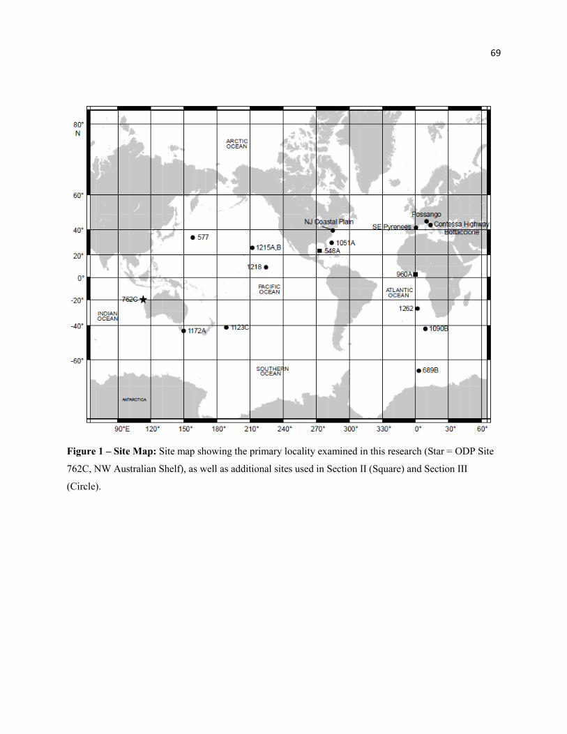
69

Figure 1 – Site Map: Site map showing the primary locality examined in this research (Star = ODP Site

762C, NW Australian Shelf), as well as additional sites used in Section II (Square) and Section III

(Circle).

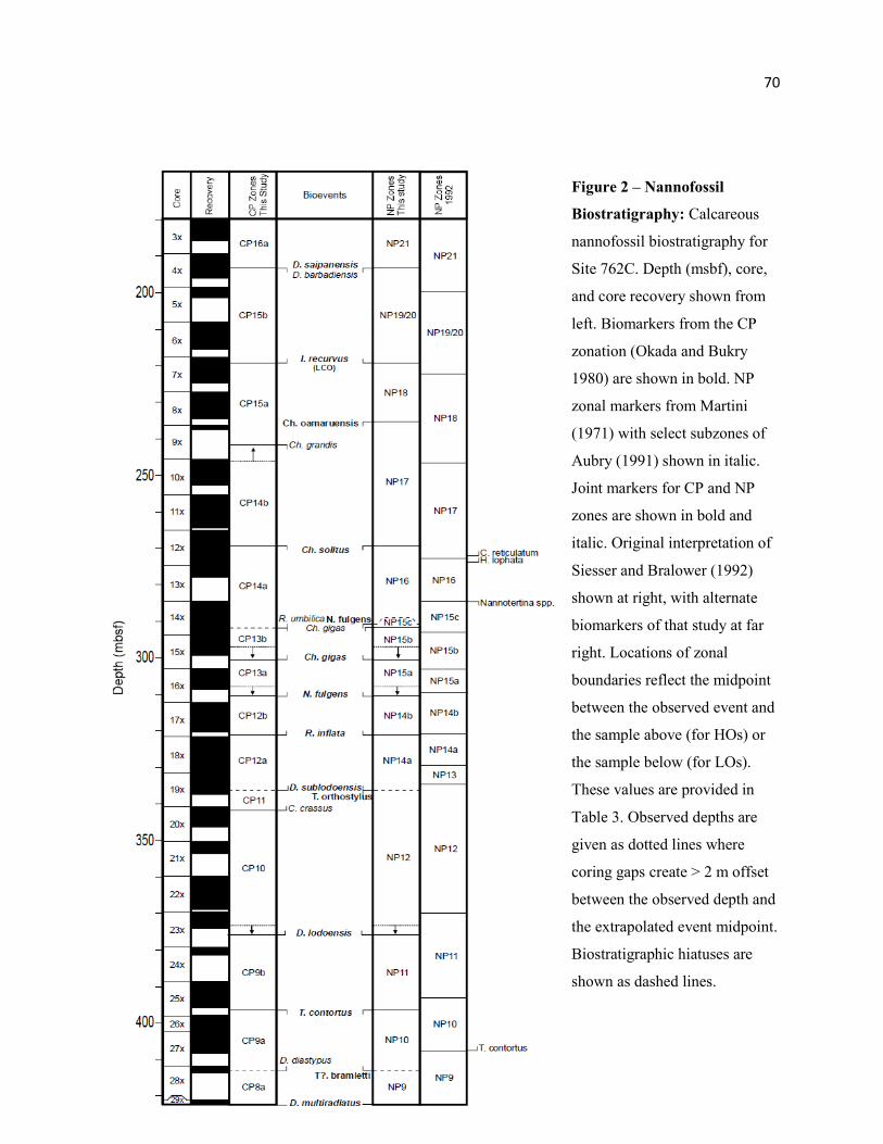
70

Figure 2 – Nannofossil

Biostratigraphy: Calcareous

nannofossil biostratigraphy for

Site 762C. Depth (msbf), core,

and core recovery shown from

left. Biomarkers from the CP

zonation (Okada and Bukry

1980) are shown in bold. NP

zonal markers from Martini

(1971) with select subzones of

Aubry (1991) shown in italic.

Joint markers for CP and NP

zones are shown in bold and

italic. Original interpretation of

Siesser and Bralower (1992)

shown at right, with alternate

biomarkers of that study at far

right. Locations of zonal

boundaries reflect the midpoint

between the observed event and

the sample above (for HOs) or

the sample below (for LOs).

These values are provided in

Table 3. Observed depths are

given as dotted lines where

coring gaps create > 2 m offset

between the observed depth and

the extrapolated event midpoint.

Biostratigraphic hiatuses are

shown as dashed lines.

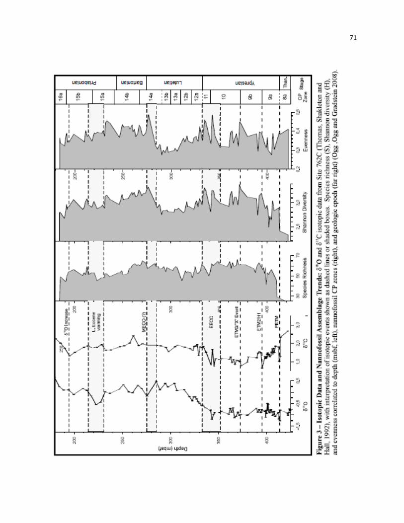
71

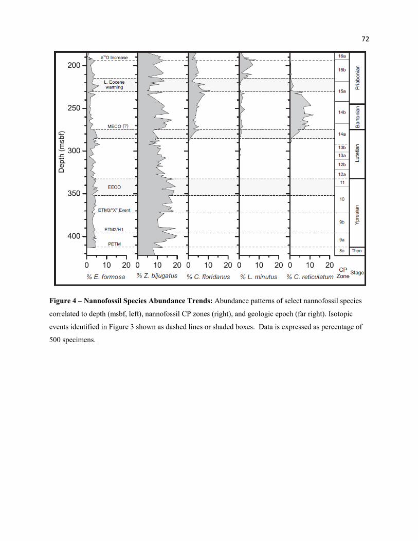
72

Figure 4 – Nannofossil Species Abundance Trends: Abundance patterns of select nannofossil species

correlated to depth (msbf, left), nannofossil CP zones (right), and geologic epoch (far right). Isotopic

events identified in Figure 3 shown as dashed lines or shaded boxes. Data is expressed as percentage of

500 specimens.

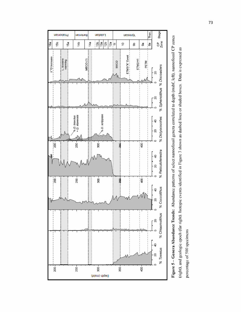
73

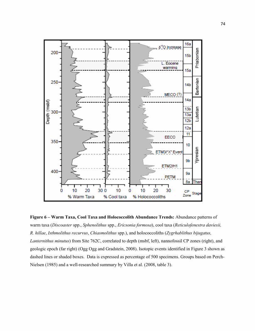
74

Figure 6 – Warm Taxa, Cool Taxa and Holococcolith Abundance Trends: Abundance patterns of

warm taxa (Discoaster spp., Sphenolithus spp., Ericsonia formosa), cool taxa (Reticulofenestra daviesii,

R. hillae, Isthmolithus recurvus, Chiasmolithus spp.), and holococcoliths (Zygrhablithus bijugatus,

Lanternithus minutus) from Site 762C, correlated to depth (msbf, left), nannofossil CP zones (right), and

geologic epoch (far right) (Ogg Ogg and Gradstein, 2008). Isotopic events identified in Figure 3 shown as

dashed lines or shaded boxes. Data is expressed as percentage of 500 specimens. Groups based on Perch-

Nielsen (1985) and a well-researched summary by Villa et al. (2008, table 3).

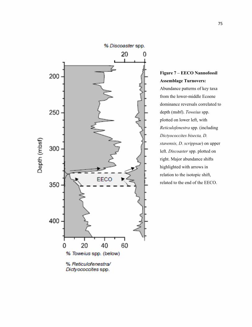
75

Figure 7 – EECO Nannofossil

Assemblage Turnovers:

Abundance patterns of key taxa

from the lower-middle Ecoene

dominance reversals correlated to

depth (msbf). Toweius spp.

plotted on lower left, with

Reticulofenestra spp. (including

Dictyococcites bisecta, D.

stavensis, D. scrippsae) on upper

left. Discoaster spp. plotted on

right. Major abundance shifts

highlighted with arrows in

relation to the isotopic shift,

related to the end of the EECO.

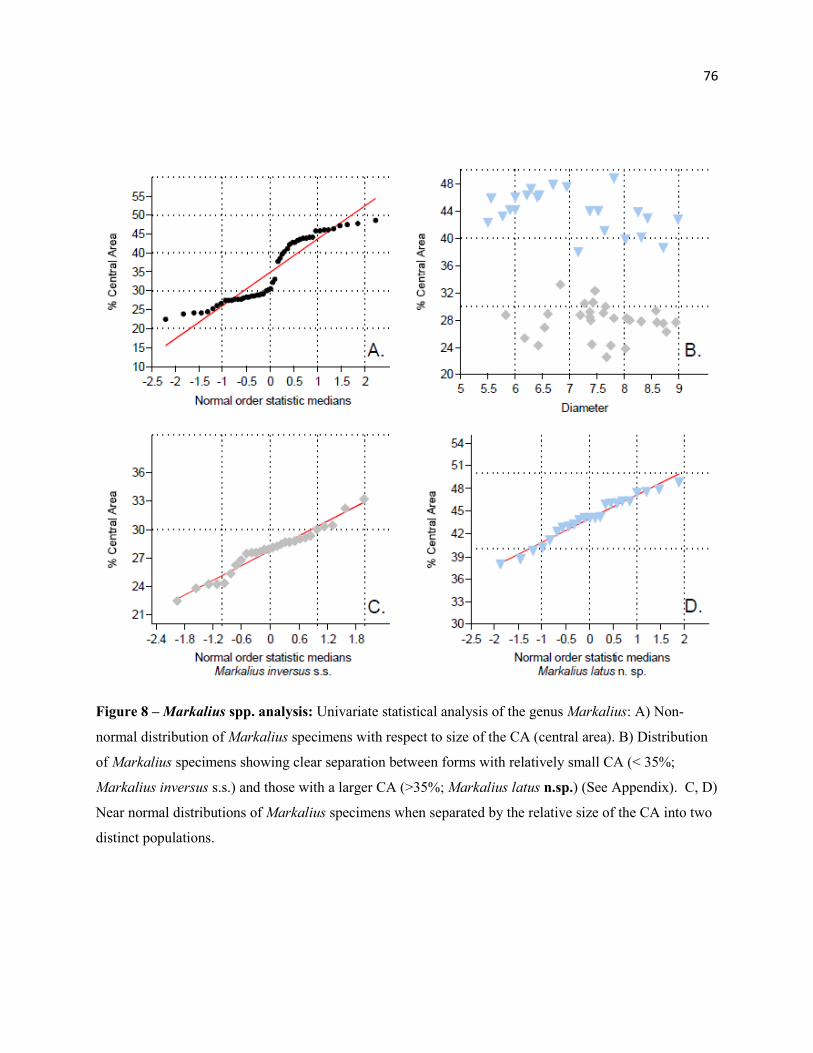
76

Figure 8 – Markalius spp. analysis: Univariate statistical analysis of the genus Markalius: A) Non-

normal distribution of Markalius specimens with respect to size of the CA (central area). B) Distribution

of Markalius specimens showing clear separation between forms with relatively small CA (< 35%;

Markalius inversus s.s.) and those with a larger CA (>35%; Markalius latus n.sp.) (See Appendix). C, D)

Near normal distributions of Markalius specimens when separated by the relative size of the CA into two

distinct populations.

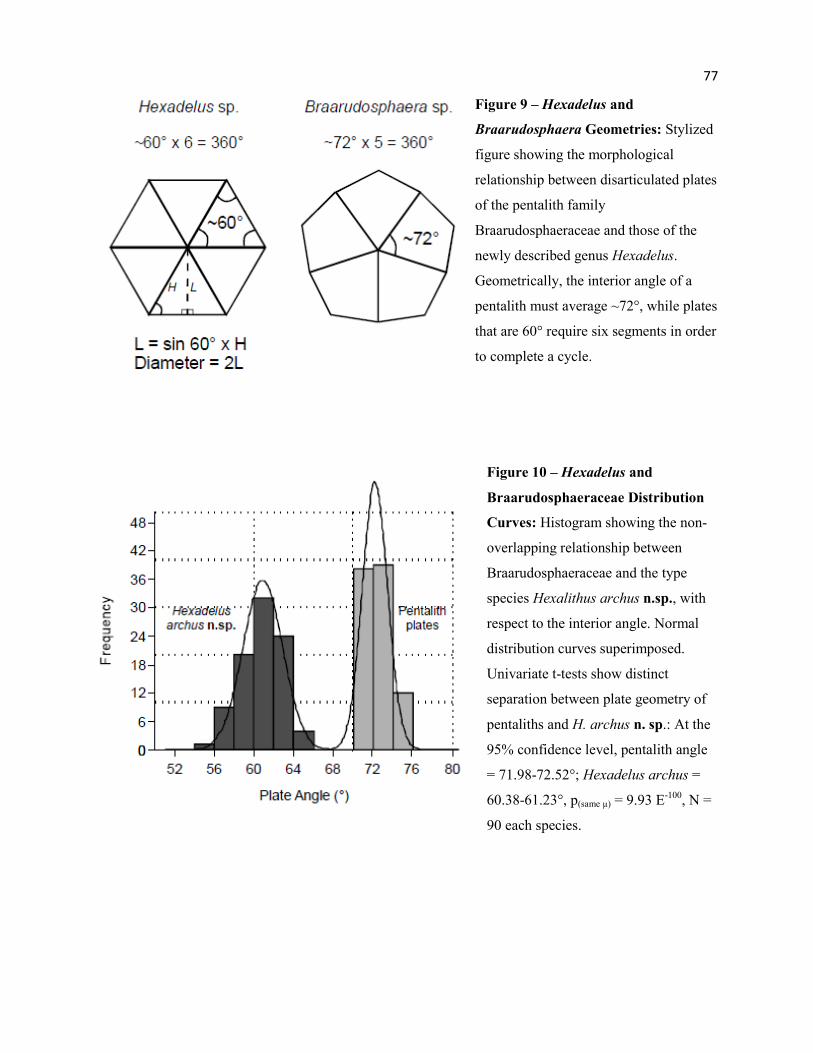
77

Figure 9 – Hexadelus and

Braarudosphaera Geometries: Stylized

figure showing the morphological

relationship between disarticulated plates

of the pentalith family

Braarudosphaeraceae and those of the

newly described genus Hexadelus.

Geometrically, the interior angle of a

pentalith must average ~72°, while plates

that are 60° require six segments in order

to complete a cycle.

Figure 10 – Hexadelus and

Braarudosphaeraceae Distribution

Curves: Histogram showing the non-

overlapping relationship between

Braarudosphaeraceae and the type

species Hexalithus archus n.sp., with

respect to the interior angle. Normal

distribution curves superimposed.

Univariate t-tests show distinct

separation between plate geometry of

pentaliths and H. archus n. sp.: At the

95% confidence level, pentalith angle

= 71.98-72.52°; Hexadelus archus =

60.38-61.23°, p(same µ) = 9.93 E-100, N =

90 each species.

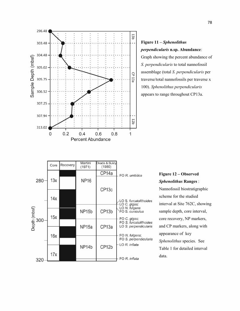
78

Figure 11 – Sphenolithus

perpendicularis n.sp. Abundance:

Graph showing the percent abundance of

S. perpendicularis to total nannofossil

assemblage (total S. perpendicularis per

traverse/total nannofossils per traverse x

100). Sphenolithus perpendicularis

appears to range throughout CP13a.

Figure 12 – Observed

Sphenolithus Ranges :

Nannofossil biostratigraphic

scheme for the studied

interval at Site 762C, showing

sample depth, core interval,

core recovery, NP markers,

and CP markers, along with

appearance of key

Sphenolithus species. See

Table 1 for detailed interval

data.

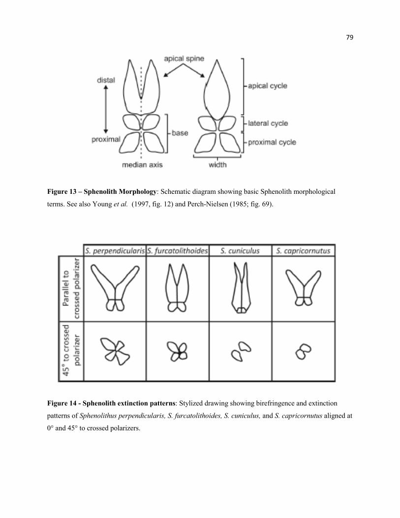
79

Figure 13 – Sphenolith Morphology: Schematic diagram showing basic Sphenolith morphological

terms. See also Young et al. (1997, fig. 12) and Perch-Nielsen (1985; fig. 69).

Figure 14 - Sphenolith extinction patterns: Stylized drawing showing birefringence and extinction

patterns of Sphenolithus perpendicularis, S. furcatolithoides, S. cuniculus, and S. capricornutus aligned at

0° and 45° to crossed polarizers.

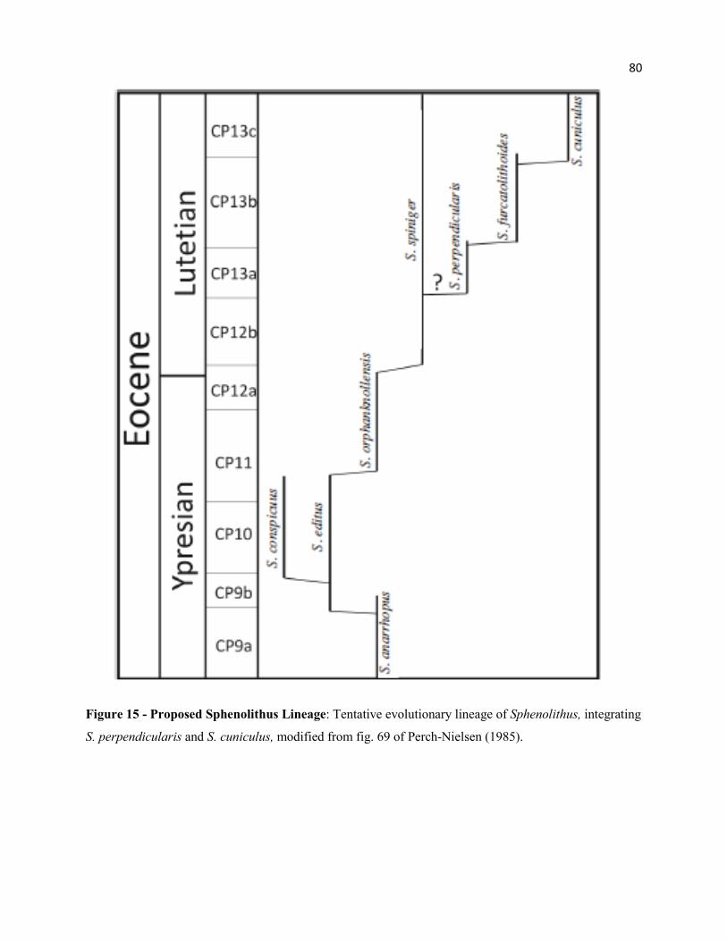
80

Figure 15 - Proposed Sphenolithus Lineage: Tentative evolutionary lineage of Sphenolithus, integrating

S. perpendicularis and S. cuniculus, modified from fig. 69 of Perch-Nielsen (1985).

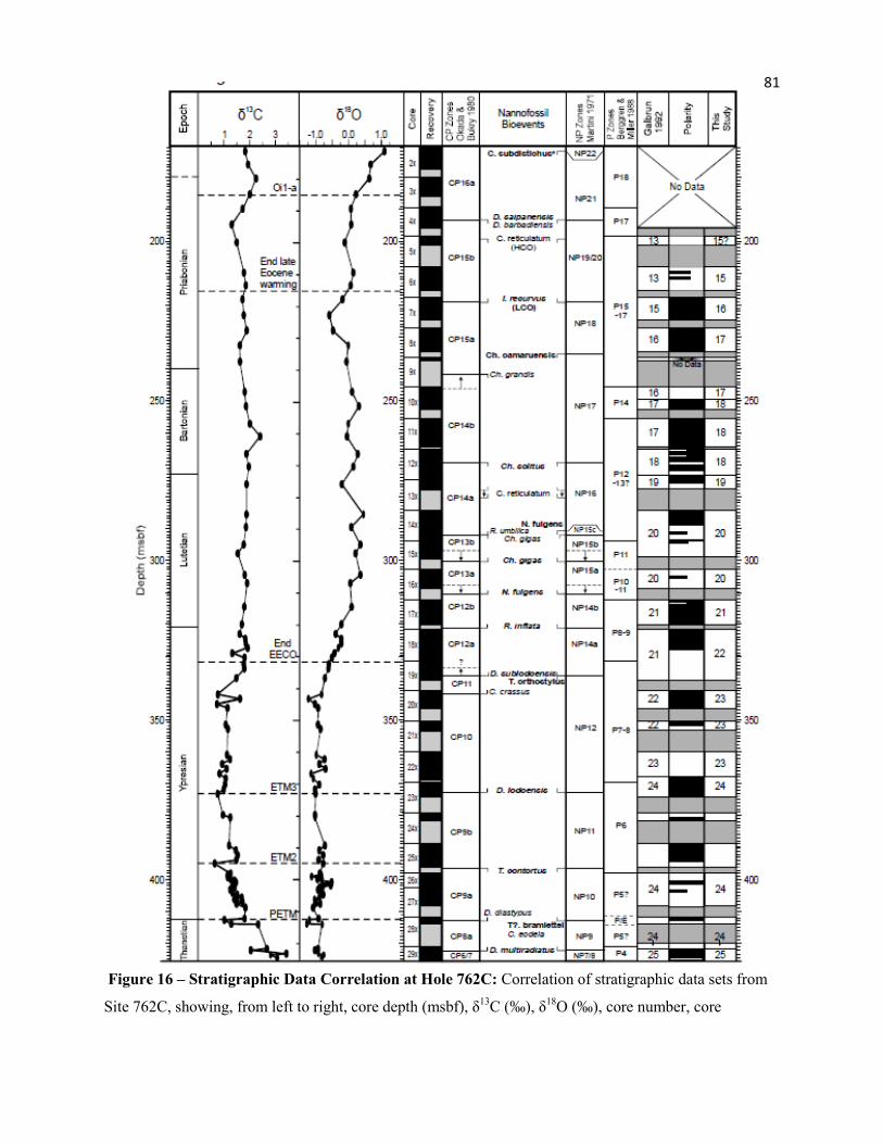
81

Figure 16 – Stratigraphic Data Correlation at Hole 762C: Correlation of stratigraphic data sets from

Site 762C, showing, from left to right, core depth (msbf), δ13C (‰), δ18O (‰), core number, core

82

recovery, calcareous nannofossil CP zonation, nannofossil bioevents, nannofossil NP zonation, planktonic

foraminiferal P zonation, magnetostratigraphy of Galbrun (1992), magnetic polarity sequence, and present

magnetostratigraphic reinterpretation. δ13C and δ18O isotopic data from Thomas Shackleton and Hall

(1992), with interpretation of isotopic events shown as dashed lines. Numbered sequence correlates to

Table 4 (column 1). CP biomarkers of Okada and Bukry (1980) in bold. NP biomarkers of Martini

(1971), with select subzones of Aubry (1991), shown in italic. Joint markers for CP and NP zones shown

in both bold and italic. Locations of CP and NP zonal boundaries reflect the midpoint between the

observed event and the sample above (for HOs) or below (for LOs). Nannofossil biozone boundaries are

shown by solid lines; however, dashed lines are used to show the observed event depth, when sample

spacing creates ≥ 2.0 m gap around the bioevent midpoint. Sample depths for nannofossil biostratigraphy

provided in Table 2. *Bioevent data from Siesser and Bralower (1992). Coring gaps are shown in grey in

both core recovery and magnetic polarity columns. Magnetic polarity indicated by black (white) fill for

normal (reverse) polarity. Revised magnetostratigraphy correlated to the GPTS of Ogg, Ogg and

Gradstein (2008).

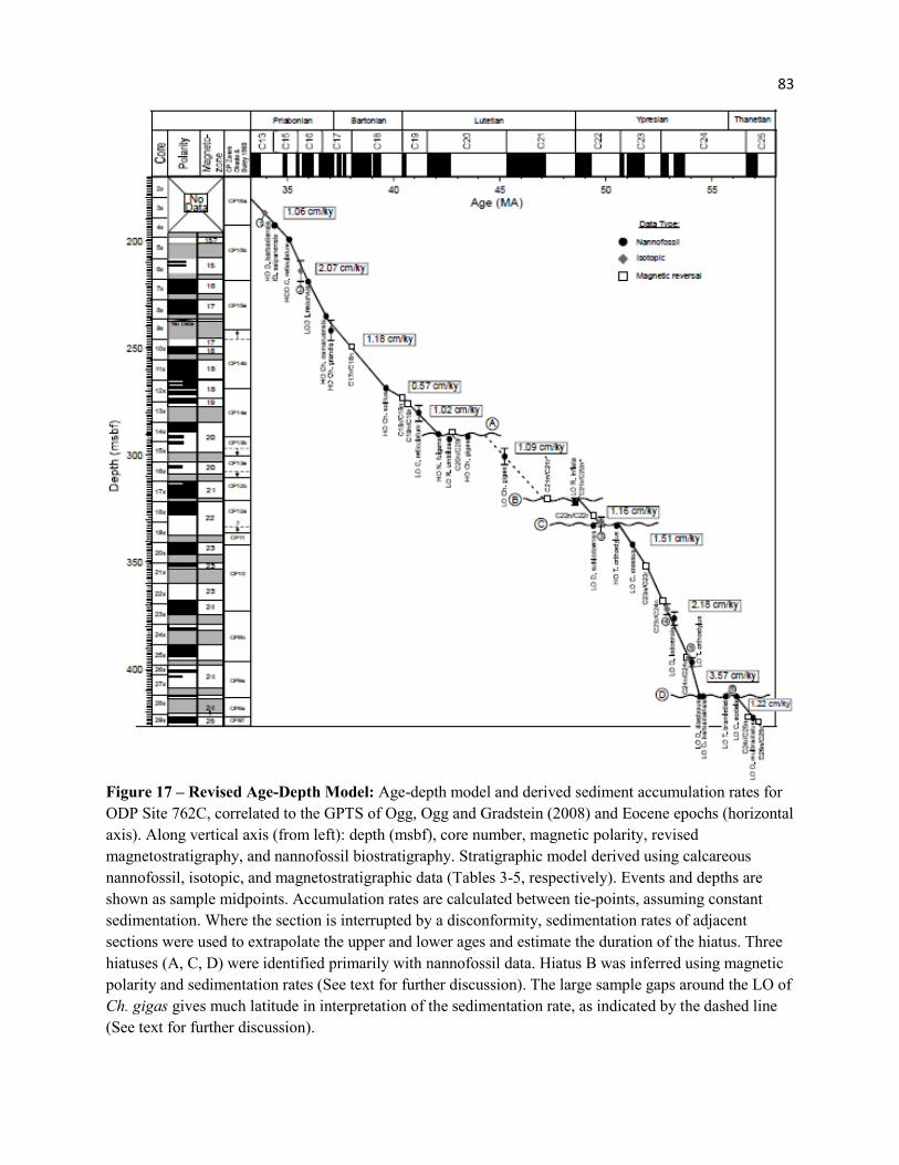
83

Figure 17 – Revised Age-Depth Model: Age-depth model and derived sediment accumulation rates for ODP Site 762C, correlated to the GPTS of Ogg, Ogg and Gradstein (2008) and Eocene epochs (horizontal axis). Along vertical axis (from left): depth (msbf), core number, magnetic polarity, revised magnetostratigraphy, and nannofossil biostratigraphy. Stratigraphic model derived using calcareous nannofossil, isotopic, and magnetostratigraphic data (Tables 3-5, respectively). Events and depths are shown as sample midpoints. Accumulation rates are calculated between tie-points, assuming constant sedimentation. Where the section is interrupted by a disconformity, sedimentation rates of adjacent sections were used to extrapolate the upper and lower ages and estimate the duration of the hiatus. Three hiatuses (A, C, D) were identified primarily with nannofossil data. Hiatus B was inferred using magnetic polarity and sedimentation rates (See text for further discussion). The large sample gaps around the LO of Ch. gigas gives much latitude in interpretation of the sedimentation rate, as indicated by the dashed line (See text for further discussion).

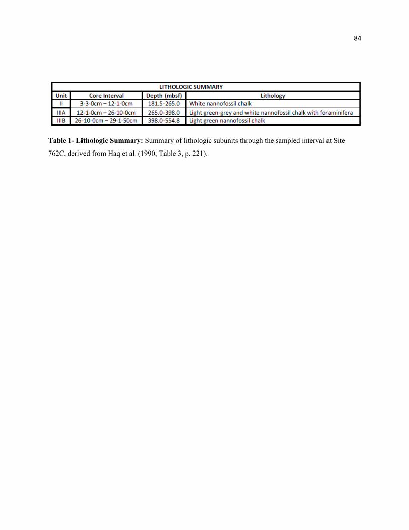
84

Table 1- Lithologic Summary: Summary of lithologic subunits through the sampled interval at Site

762C, derived from Haq et al. (1990, Table 3, p. 221).

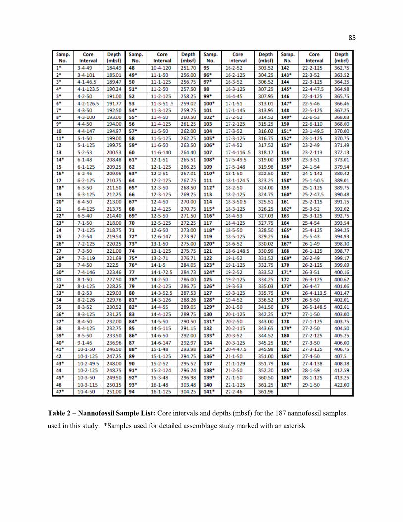
85

Table 2 – Nannofossil Sample List: Core intervals and depths (mbsf) for the 187 nannofossil samples

used in this study. *Samples used for detailed assemblage study marked with an asterisk

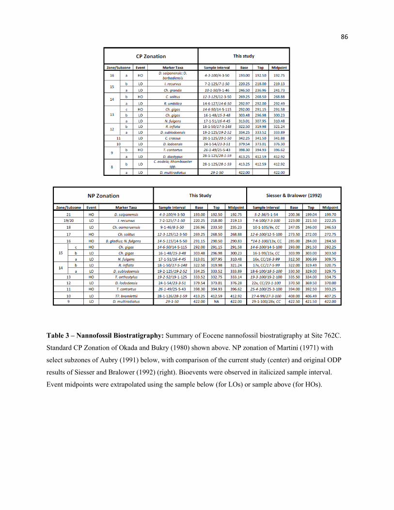
86

Table 3 – Nannofossil Biostratigraphy: Summary of Eocene nannofossil biostratigraphy at Site 762C.

Standard CP Zonation of Okada and Bukry (1980) shown above. NP zonation of Martini (1971) with

select subzones of Aubry (1991) below, with comparison of the current study (center) and original ODP

results of Siesser and Bralower (1992) (right). Bioevents were observed in italicized sample interval.

Event midpoints were extrapolated using the sample below (for LOs) or sample above (for HOs).

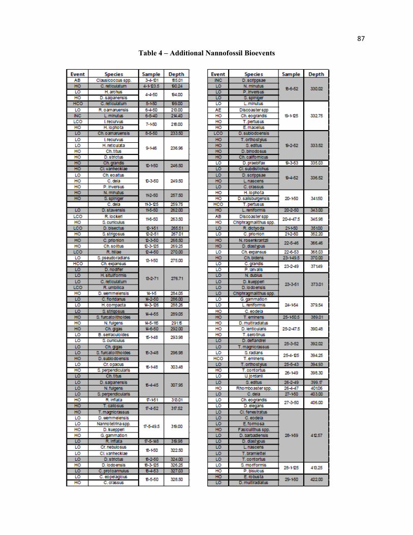
87

Table 4 – Additional Nannofossil Bioevents

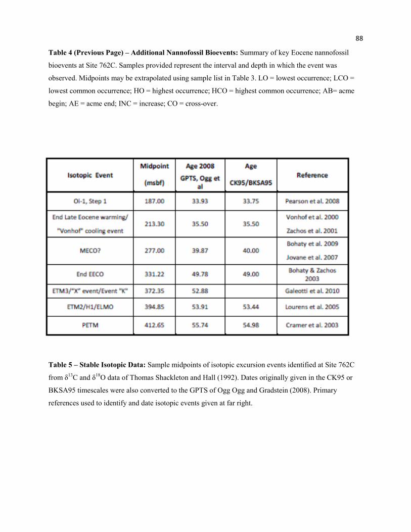
88

Table 4 (Previous Page) – Additional Nannofossil Bioevents: Summary of key Eocene nannofossil

bioevents at Site 762C. Samples provided represent the interval and depth in which the event was

observed. Midpoints may be extrapolated using sample list in Table 3. LO = lowest occurrence; LCO =

lowest common occurrence; HO = highest occurrence; HCO = highest common occurrence; AB= acme

begin; AE = acme end; INC = increase; CO = cross-over.

Table 5 – Stable Isotopic Data: Sample midpoints of isotopic excursion events identified at Site 762C

from δ13C and δ18O data of Thomas Shackleton and Hall (1992). Dates originally given in the CK95 or

BKSA95 timescales were also converted to the GPTS of Ogg Ogg and Gradstein (2008). Primary

references used to identify and date isotopic events given at far right.

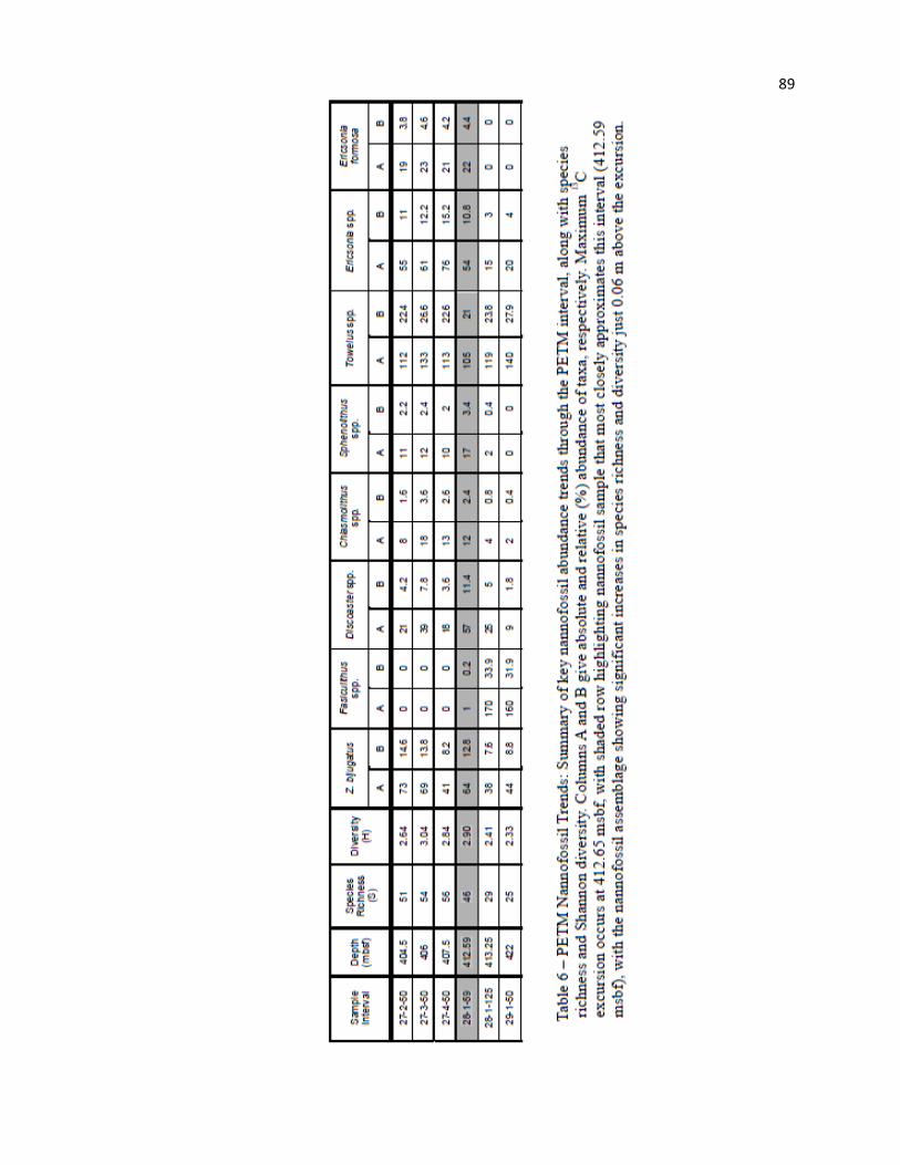
89

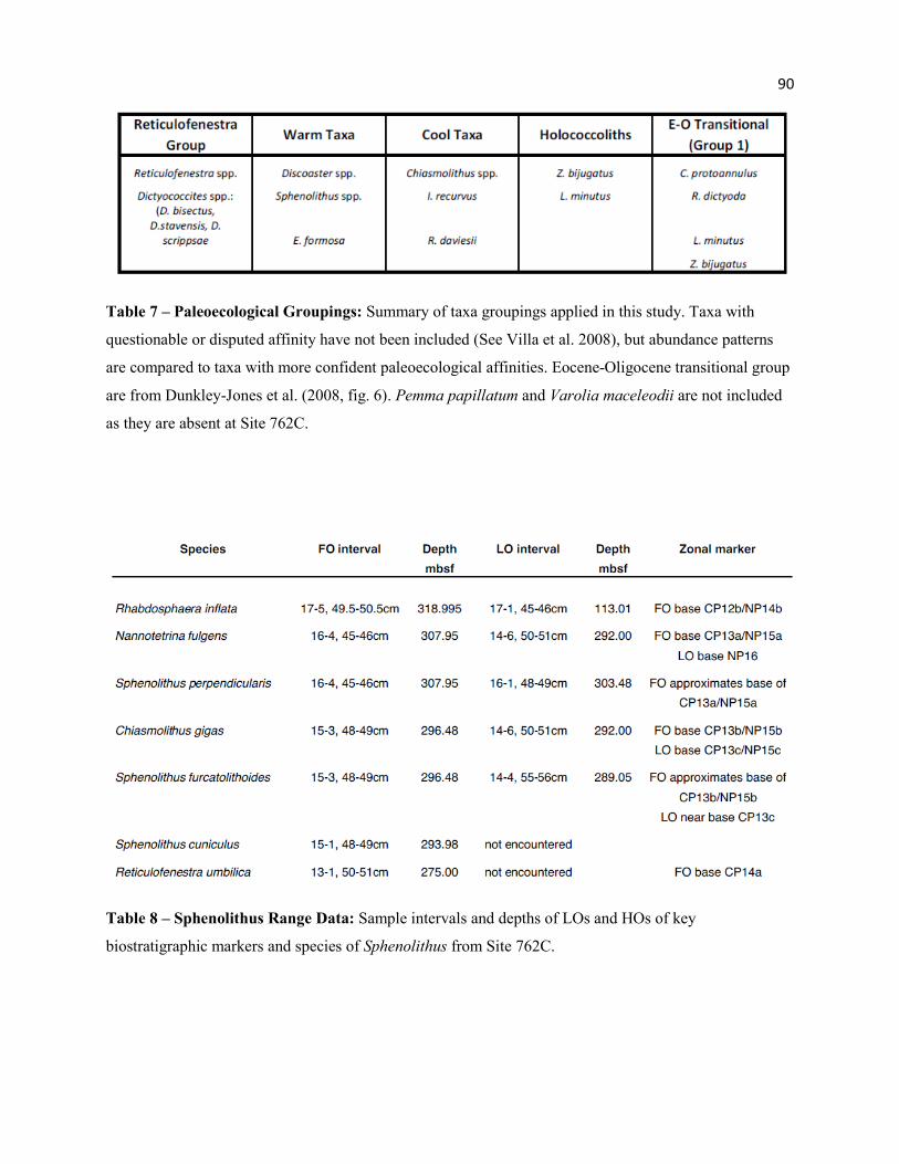
90

Table 7 – Paleoecological Groupings: Summary of taxa groupings applied in this study. Taxa with

questionable or disputed affinity have not been included (See Villa et al. 2008), but abundance patterns

are compared to taxa with more confident paleoecological affinities. Eocene-Oligocene transitional group

are from Dunkley-Jones et al. (2008, fig. 6). Pemma papillatum and Varolia maceleodii are not included

as they are absent at Site 762C.

Table 8 – Sphenolithus Range Data: Sample intervals and depths of LOs and HOs of key

biostratigraphic markers and species of Sphenolithus from Site 762C.

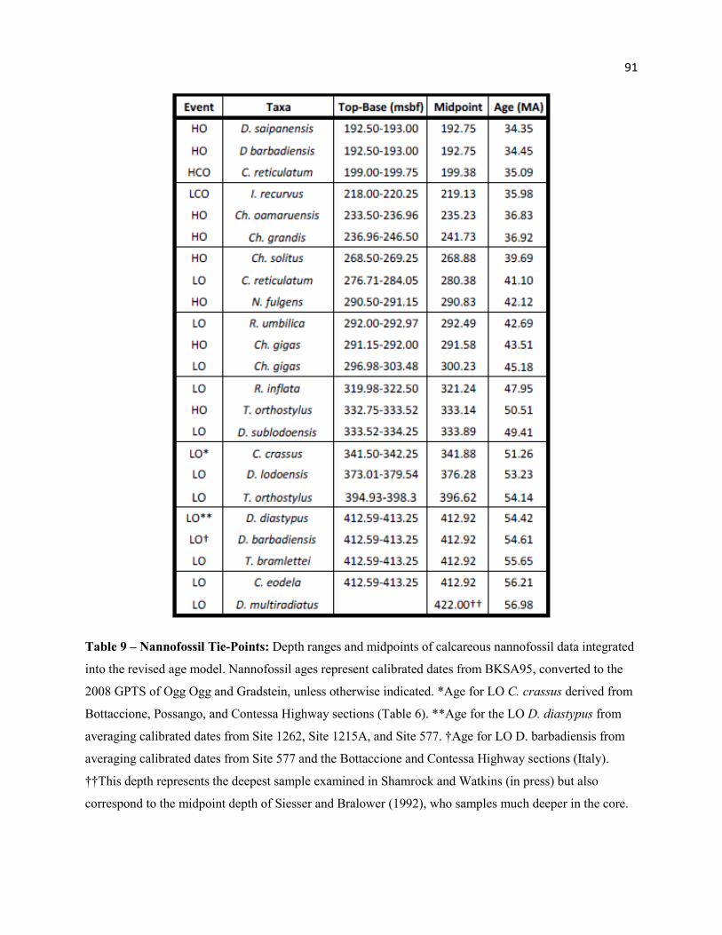
91

Table 9 – Nannofossil Tie-Points: Depth ranges and midpoints of calcareous nannofossil data integrated

into the revised age model. Nannofossil ages represent calibrated dates from BKSA95, converted to the

2008 GPTS of Ogg Ogg and Gradstein, unless otherwise indicated. *Age for LO C. crassus derived from

Bottaccione, Possango, and Contessa Highway sections (Table 6). **Age for the LO D. diastypus from

averaging calibrated dates from Site 1262, Site 1215A, and Site 577. †Age for LO D. barbadiensis from

averaging calibrated dates from Site 577 and the Bottaccione and Contessa Highway sections (Italy).

††This depth represents the deepest sample examined in Shamrock and Watkins (in press) but also

correspond to the midpoint depth of Siesser and Bralower (1992), who samples much deeper in the core.

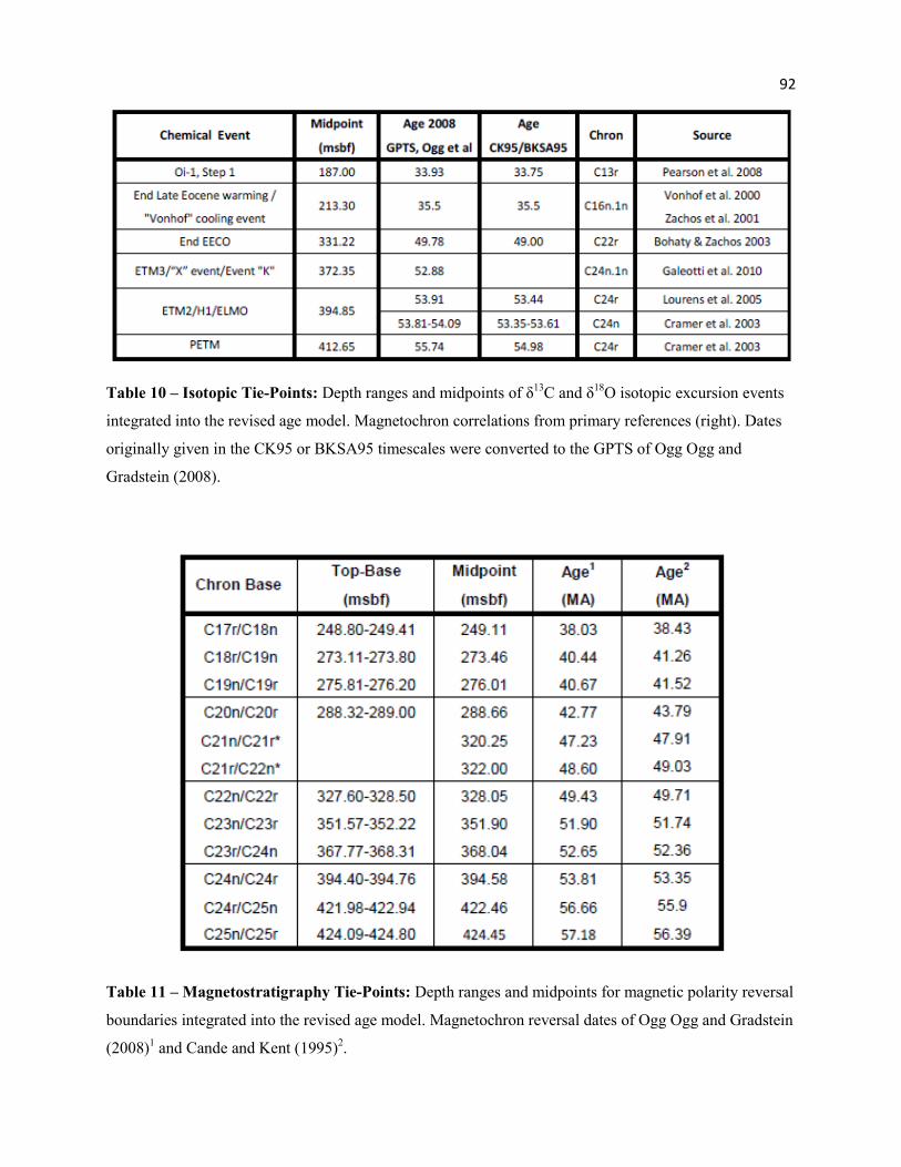
92

Table 10 – Isotopic Tie-Points: Depth ranges and midpoints of δ13C and δ18O isotopic excursion events

integrated into the revised age model. Magnetochron correlations from primary references (right). Dates

originally given in the CK95 or BKSA95 timescales were converted to the GPTS of Ogg Ogg and

Gradstein (2008).

Table 11 – Magnetostratigraphy Tie-Points: Depth ranges and midpoints for magnetic polarity reversal

boundaries integrated into the revised age model. Magnetochron reversal dates of Ogg Ogg and Gradstein

(2008)1 and Cande and Kent (1995)2.

93

Table 12 – Nannofossil Event Ages (Following two pages): Summary of derived ages for nannofossil

bioevents at Site 762C based on the revised age model, compared to the BSKA95 and several additional,

globally distributed sites. Midpoints for Site 762C are extrapolated using sample list in Table 1. Published

and extrapolated ages of calcareous nannofossil bioevents are recalibrated to the GPTS of Ogg Ogg and

Gradstein (2008). LO = lowest occurrence; LCO = lowest common occurrence; LRO = lowest rare

occurrence; HO = highest occurrence; HCO = highest common occurrence; AB = acme begin; AE = acme

end; CO = cross-over. Bioevents representing the HCO or LCO for a particular taxa are given in italic.

The lowest rare occurrence (LRO), a designation not used in this study but in others, is shown in bold.

Events located within a hiatus cannot be accurately dated, are indicated by UNC.

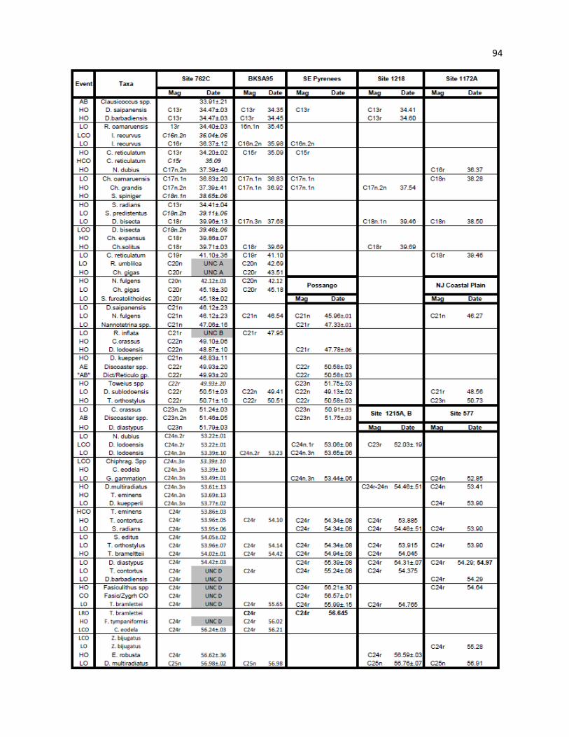
94

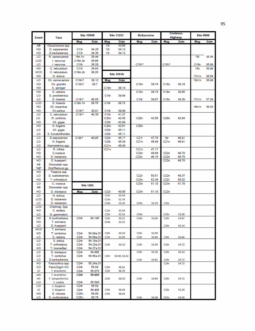
95

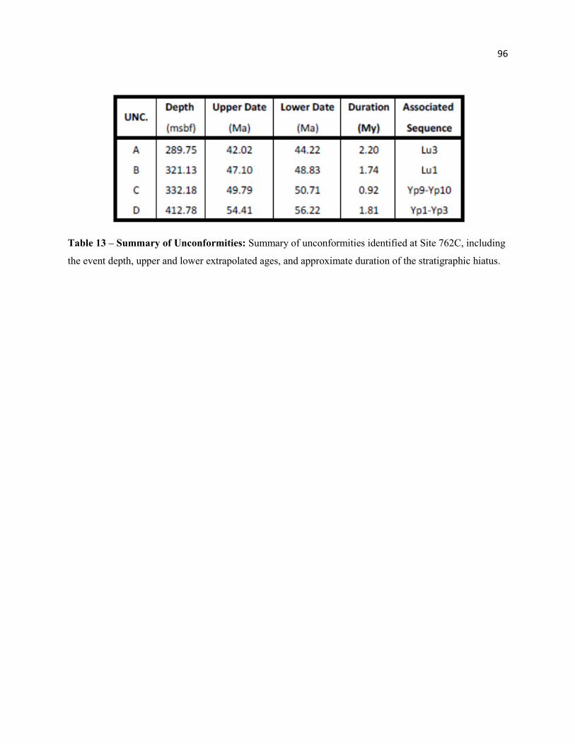
96

Table 13 – Summary of Unconformities: Summary of unconformities identified at Site 762C, including

the event depth, upper and lower extrapolated ages, and approximate duration of the stratigraphic hiatus.

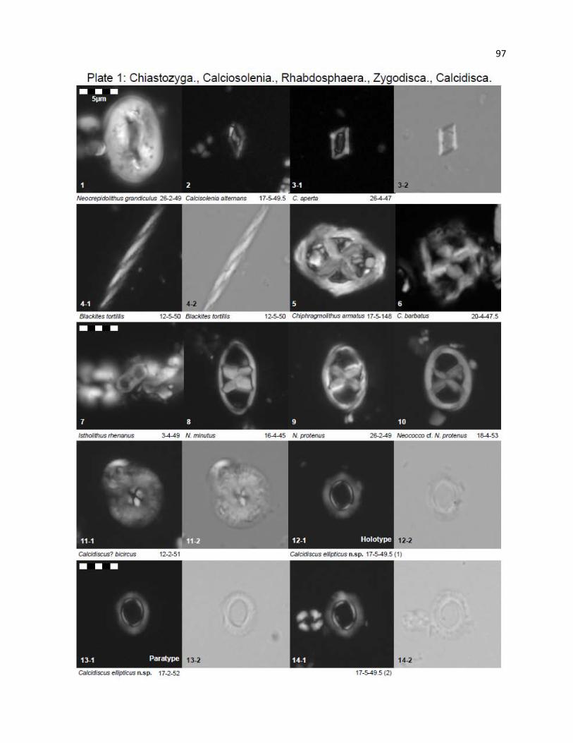
97

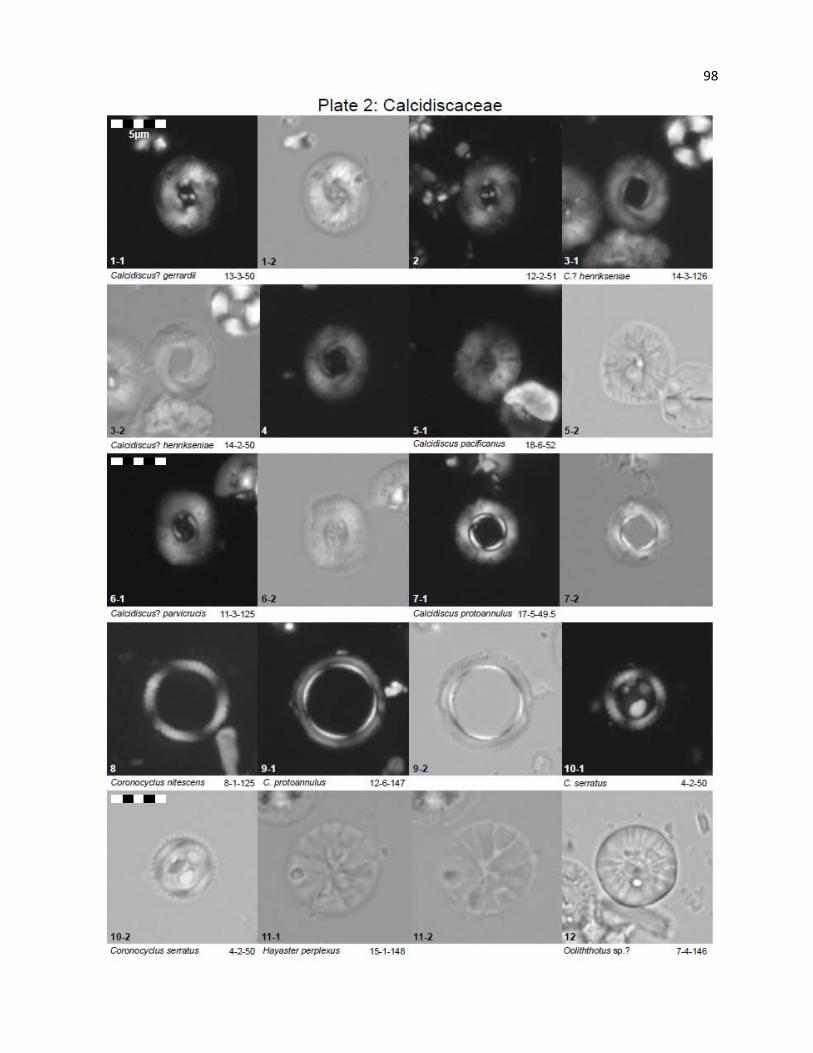
98

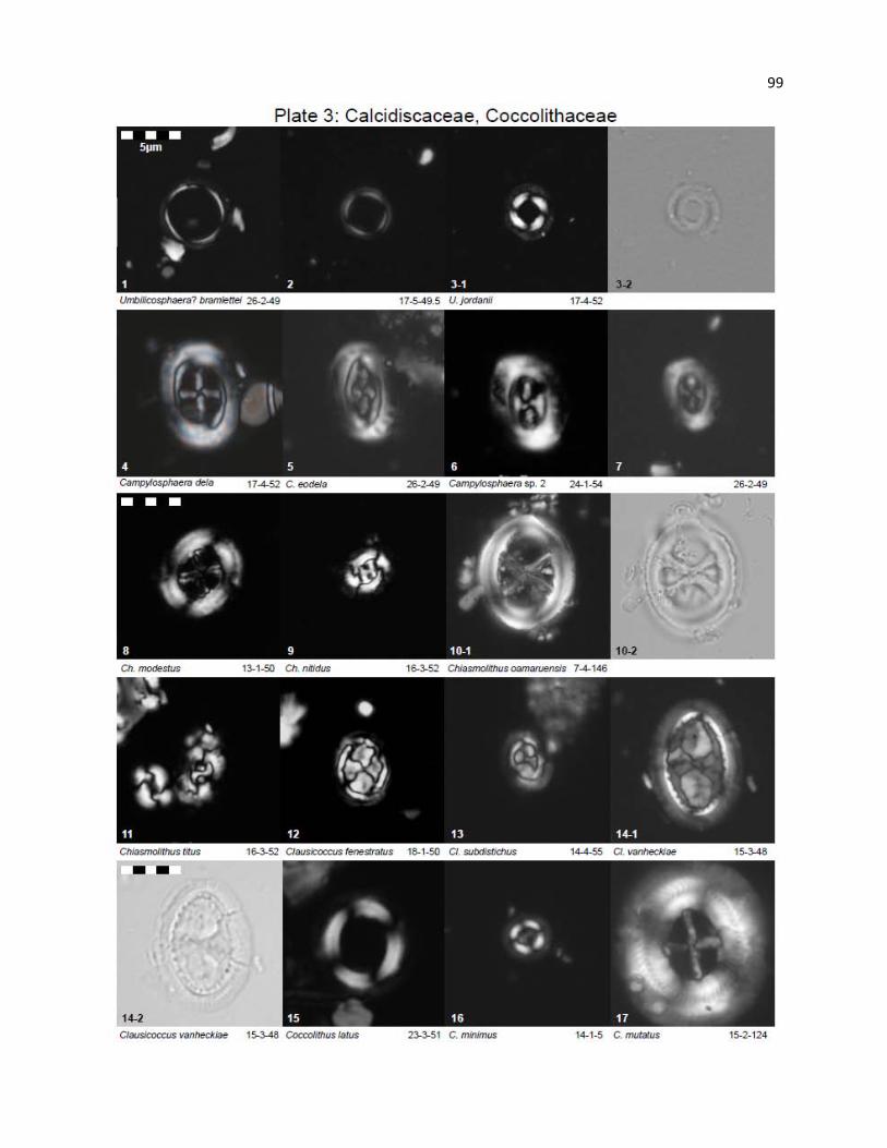
99

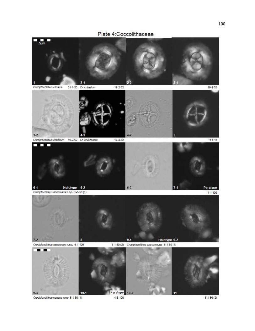
100

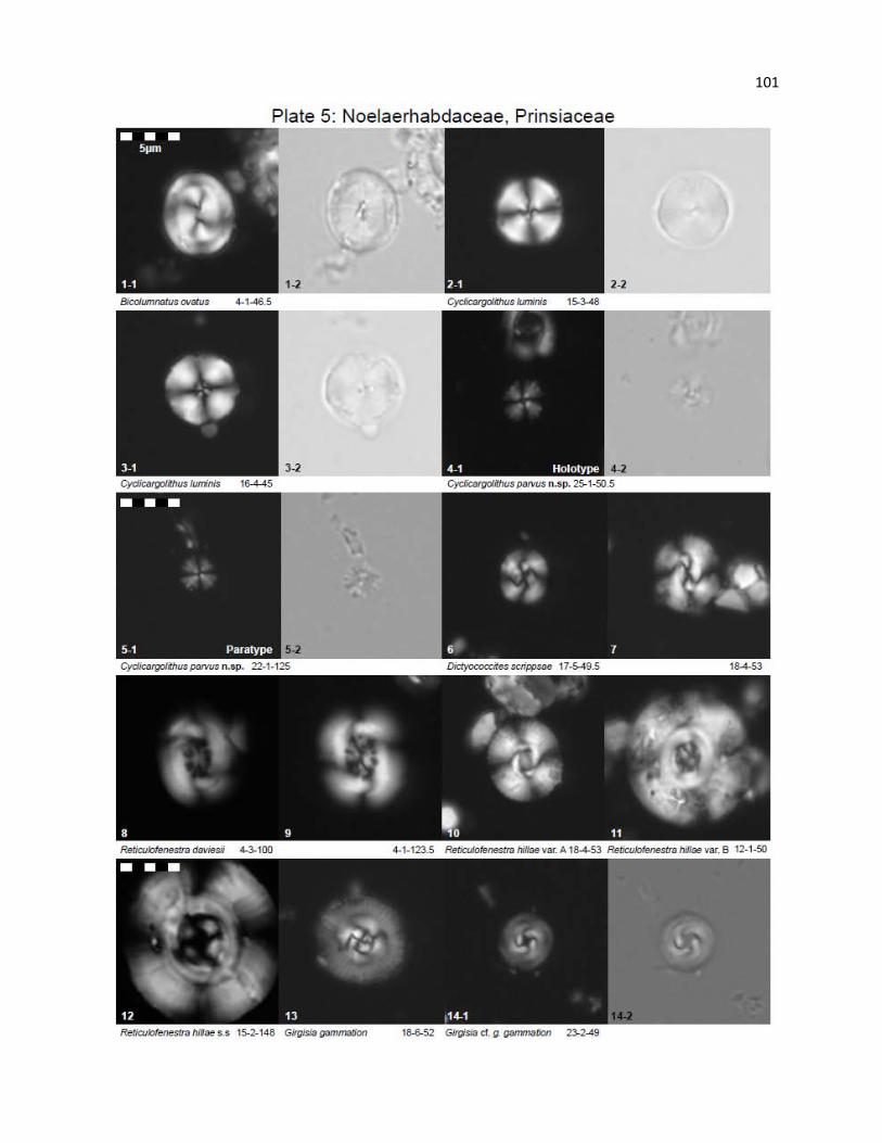
101

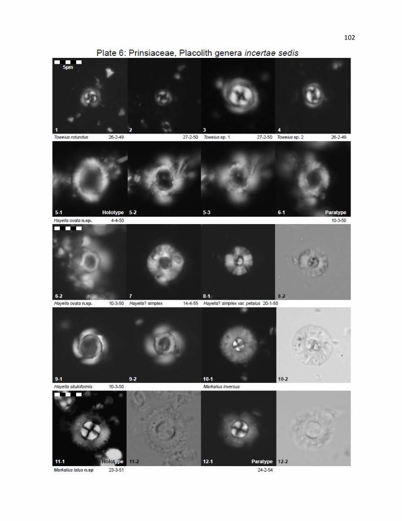
102

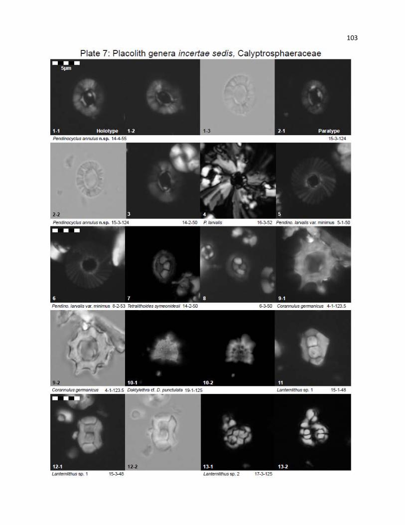
103

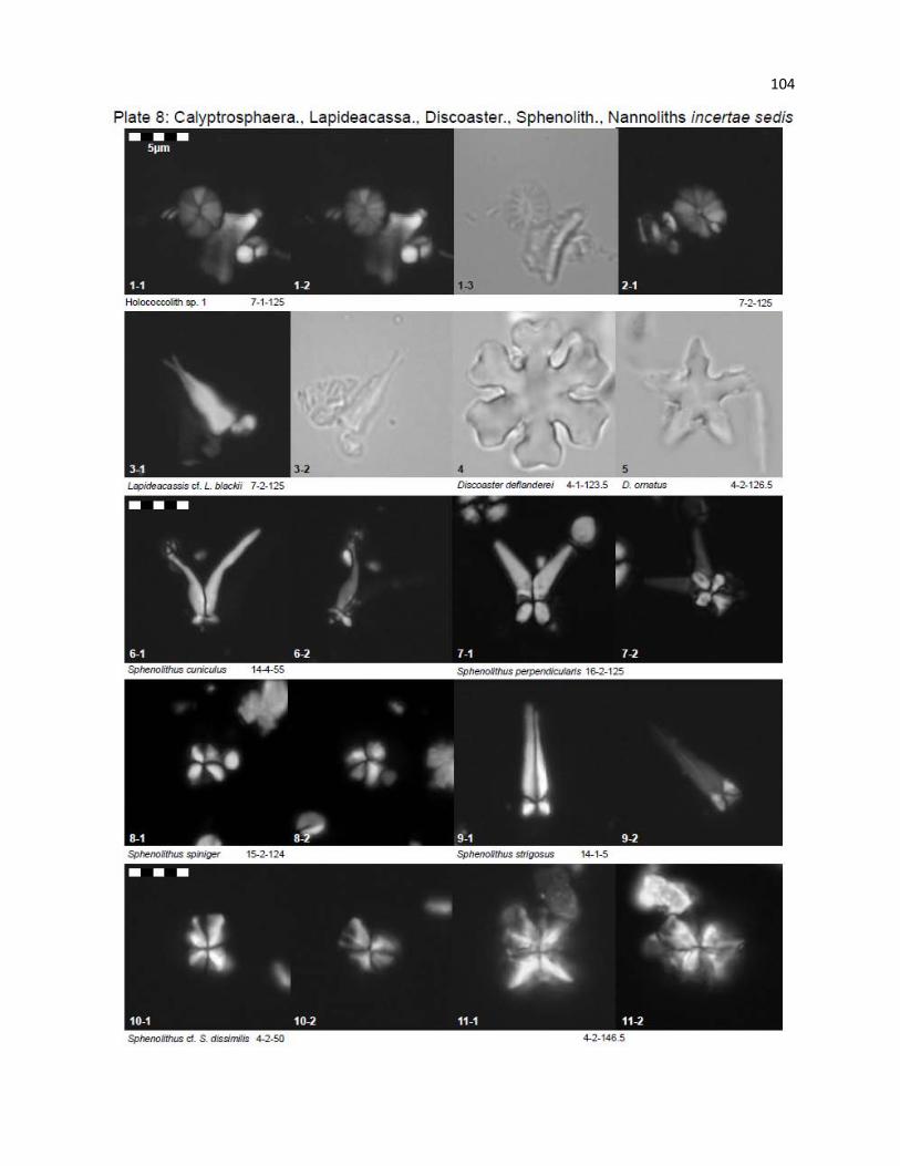
104

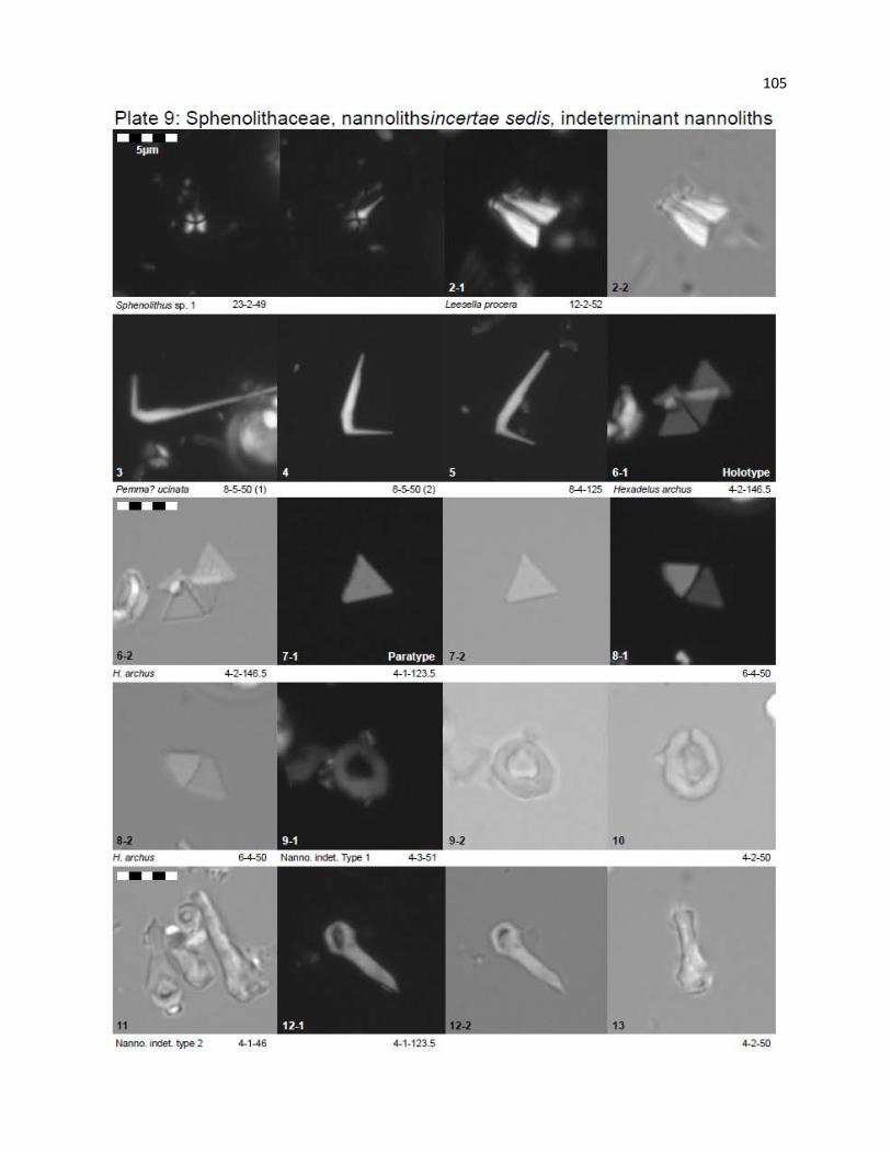
105

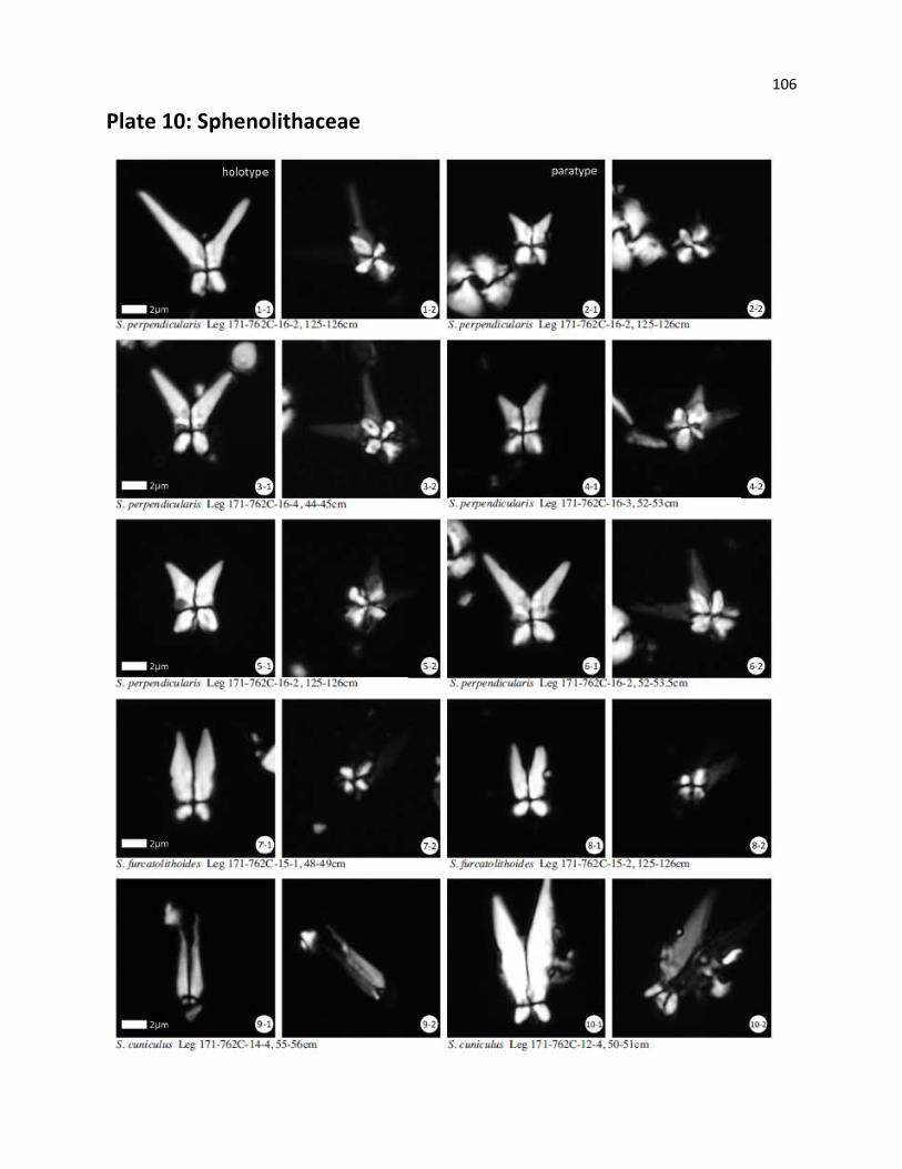
106

Plate 10: Sphenolithaceae

107

APPENDIX A - CALCAREOUS NANNOFOSSIL SYSTEMATIC PALEONTOLOGY AND

TAXONOMIC APPENDIX

Taxonomic and/or stratigraphic notes are gives for all species identified within the section.

Notable abundance trends are given for individual species; however, genus and family level abundance

trends are treated above. Nannofossil terminology follows guidelines provided in Young et al. (1997).

Recent research on Eocene cores from Tanzania by Bown (2005), Bown and Dunkley-Jones

(2006), and Bown, Dunkley-Jones and Young (2007) has generated a significant image atlas, and

numerous taxonomic points have been addressed in these works that will not be reiterated here. We

restrict our main discussion and imaging to species that were not addressed, recently named species, or

where opinions on taxonomy diverge. Many species that are recently named are shown in XPL (Cross-

polarized light) only, as they are well illustrated in the original descriptions. Where two images are

provided for one specimen, XPL is always shown before PL (Plane-polarized light).

Numerous new species were recently identified by Bown (2005), Bown and Dunkley-Jones

(2006) and Bown, Dunkley-Jones and Young (2007). Many of these species were observed in the

Exmouth section; however, observed ranges of several species extend above and/or below those provided

in the original descriptions. A significant portion of such range extensions are likely due to coring gaps in

the Tanzania section (Bown 2005, fig 2; Bown, Dunkley-Jones and Young 2007, fig. 1). To limit

redundancy, we do not treat each range issue separately, but refer the reader to these publications for

independent comparison.

MUROLITHS

Order EIFFELLITHALES Rood, et al., 1971

Family CHIASTOZYGACEAE Rood, et al., 1973

Neocrepidolithus grandiculus Bown 2005

Plate 1-1; Observed range: CP9a-13a, NP10-15a

Jakubowskia leoniae Varol 1989

Observed range: CP9a-12a; NP10-14a

Order SYRACOSPHAERALES Hay 1977, emend. Young et al., 2003

Family CALCIOSOLENIACEAE Kamptner 1927

Calciosolenia alternans Bown and Dunkley-Jones 2006

Plate 1-2; Observed range: CP12a; NP14a

108

Calciosolenia aperta (Hay & Mohler 1967) Bown 2005

Plate 1-3 Observed range: CP9b, NP11

Family RHABDOSPHAERACEAE Haeckel 1894

Most species of Blackites and Rhabdosphaera were extremely rare at the locality.

Blackites gracilentus Bown and Dunkley-Jones 2006

Observed range: CP14b; NP17

Blackites morionum (Deflandre in Deflandre and Fert 1954) Varol 1989

Observed range: CP9a; NP10

Blackites perlongus (Deflandre in Grassé 1952) Bramlette and Sullivan 1961

Observed range: CP9b; NP11

Blackites spinosus (Deflandre and Fert 1954) Hay and Towe 1962 / Rhabdosphaera tenuis Bramlette and

Sullivan 1961

The vast majority of specimens are incomplete, lacking their diagnostic base. As a result, B.

spinosus has been grouped with R. tenuis, though this diminishes the biostratigraphic utility. This group is

most abundant in CP10. Observed range: CP9a-16a; NP10-21

Blackites tortillis Bown and Dunkley-Jones 2006

Plate 1-4; The observed LO occurs in mid-CP14a. Observed range: CP14a-15b; NP16-19/20

Rhabdosphaera inflata Bramlette and Sullivan 1961

Observed range: CP12b; NP14b

Rhabdopshaera sola Perch-Nielsen 1971

Observed range: CP9b-10; NP11-12

Rhabdosphaera tenuis Bramlette and Sullivan 1961

See B. spinosus/R. tenuis, above.

Rhabdosphaera truncata Bramlette and Sullivan 1961

Observed range: CP9b-12a; NP11-13

Family SYRACOSPHAERACEAE Hay 1977

Syracosphaera Lohmann 1902

Specimens of this genus were rare and sporadic throughout the section and have been grouped as

Syracosphaera spp. for statistical analysis. Observed range: CP9a-16a; NP10-21

Order ZYGODISCALES Young and Bown 1997

Family HELICOSPHAERACEAE Black 1971

Most species of the genus Helicosphaera were rare and sporadic, though the genus as a whole becomes

fairly common and consistent in the Upper Eocene. Average relative abundance = ~0.5% from the genus LO

through CP15b, but increases at the base of CP16a (µ = 1.6%, Max. = 4.0%)

109

Helicosphaera bramlettei (Müller 1970) Jafar and Martini 1975

Observed range: CP14a-16a; NP16-21

Helicosphaera compacta Bramlette and Wilcoxon 1967

The LCO occurs in CP14b at this site, with a notable abundance increase in upper CP15b, also

shown in Wei and Wise (1990a). Observed range: CP14a?-16a; NP16-21

Helicosphaera dinesenii (Perch-Nielsen 1971) Jafar and Martini 1975

Observed range: CP13a-14a; NP15a-16

Helicosphaera heezenii (Bukry 1971) Jafar and Martini 1975

Observed range: CP13b-14b; NP15b-17

Helicosphaera lophota (Bramlette and Sullivan 1961) Jafar and Martini 1975

LO occurs at the base of CP11, with HO at the base of CP15b. Observed range: CP10-15b; NP12-

19/20

Helicosphaera papillata (Bukry and Bramlette 1969) Jafar and Martini 1975

The HO occurs just above base of CP12b. Observed range: CP12a-12b; NP14a-14b

Helicosphaera reticulata Bramlette and Wilcoxon 1967

Observed range: CP15a-16a; NP18-21

Helicosphaera salebrosa Perch-Nielsen 1971

Observed range: CP13b-15b; NP15b-19/20

Helicosphaera seminulum (Bramlette and Sulllivan 1961) Jafar and Martini 1975

Observed range: CP10-15b; NP12-19/20

Helicosphaera wilcoxonii (Gartner 1971) Jafar and Martini 1975

Observed range: CP14b-16a; NP17-21

Family PONTOSPHAERACEAE Lemmermann 1908

The genera Pontosphaera and Transversopontis were observed throughout the section from CP8a-16a.

Specimens were generally rare and sporadic at this locality, so were grouped together as Pontosphaera spp. for data

analysis. Though detailed biostratigraphic analysis was not conducted on individual species within these two genera,

species that were identified are listed below.

Pontosphaera formosa (Bukry and Bramlette 1968) Romein 1979

Pontosphaera multipora (Kamptner 1948) Roth 1970, emend. Burns 1973

Pontosphaera pectinata (Bramlette and Sullivan 1961) Sherwood 1974

Pontosphaera plana (Bramlette and Sullivan 1961) Haq 1971

Pontosphaera versa (Bramlette and Sullivan 1961) Sherwood 1974

110

Pontosphaera rimosa (Bramlette and Sullivan 1961) Roth and Thierstein 1972

Transversopontis duocavus (Bramlette and Sullivan 1961) Locker 1973

Transversopontis exilis (Bramlette and Sullivan 1961) Perch-Nielsen 1971

Transversopontis pulcher (Deflandre in Deflandre and Fert 1954) Perch-Nielsen 1967

Transversopontis pulcheroides (Sullivan 1964) Baldi-Beke 1971

Family ZYGODISCACEAE Hay and Mohler 1967

Specimens of Chiphragmolithus spp. first occur with the LO of D. lodoensis, at the base of CP10. Some

specimens could not be differentiated to species level due to overgrowth, and have been identified simply as

Chiphragmolithus sp.

Chiphragmolithus armatus Perch-Nielsen 1971

Plate 1-5; Observed range: CP10; NP12

Chiphragmalithus barbatus Perch-Nielsen 1967

Plate 1-6; Observed range: CP9b-10; NP11-12

Chiphragmolithus calathus Bramlette and Sullivan 1961

Observed range: CP9b-10; NP11-12

Isthmolithus recurvus Deflandre in Deflandre and Fert 1954

The LCO of I. recurvus marks the base of CP15b. The LO of I. recurvus and HO of C. reticulatum

are often reported as contemporaneous markers; however, specimens of C. reticulatum are observed well

above the LO and LCO of I. recurvus. This overlap is also reported in Villa, et al. (2008), Aubry (1992),

and Wei and Wise (1990a, 1989a). Observed range: CP15a-16a; NP17-21

Isthmolithus rhenanus Martini 1973

Plate 1-7; Observed range: CP16a; NP21

Lophodolithus mochlophorus Deflandre in Deflandre and Fert 1954

Observed range: CP12a-13b; NP14a-15b

Lophodolithus nascens Bramlette and Sullivan 1961

Peak abundance occurs in CP9b-10. Observed range: CP9a-11; NP10-12

Lophodolithus reniformis Bramlette and Sullivan 1961

The LO was observed very near the CP9b/10 boundary. Observed range: CP9b-10; NP11-12

Lophodolithus rotundus Bukry and Percival 1971

Observed range: CP13a; NP15a

Neochiastozygus concinnus (Martini 1961) Perch-Nielsen 1971

The HO occurs in lower CP9b. Observed range: CP9a-9b; NP10-11

111

Neochiastozygus distentus (Bramlette and Sullivan, 1961) Perch-Nielsen 1971

Observed range: CP8a-9b; NP9-11

Neochiastozygus junctus (Bramlette and Sullivan 1961) Perch-Nielsen 1971

Observed range: CP9a-10; NP10-12

Neochiastozygus rosenkrantzii (Perch-Nielsen 1971) Varol 1989

This species was observed below the range given by Perch-Nielsen (1985) in both this study and

Bown (2005). Observed range: CP9a-10; NP10-12

Neochiastozygus substrictus Bown 2005

Observed range: CP9a-10; NP10-11

Neococcolithes dubius (Deflandre in Deflandre and Fert 1954) Black 1967

The LO is observed just below the base of CP10. Though fairly consistent in its lower range, we

observe a significant gap above CP13a, with a sporadic reappearance in CP14b prior to extinction. This

species is commonly reported through CP15a (Villa et al. 2008; Wei and Wise 1990a; Perch-Nielsen 1985);

however, Wei and Wise (1989b) also show a HO in CP14b, as at 762C. Observed range: CP9b-14b; NP11-

17

Neococcolithes minutus (Perch-Nielsen 1967) Perch-Nielsen 1971

Plate 1-8; Observed range: CP12a-14b; NP14a-17

Neococcolithes protenus (Bramlette and Sullivan 1961) Black 1967

Plate 1-9; Observed range: CP9a-10; NP10-12

Neococcolithes sp. cf. N. protenus (Bramlette and Sullivan 1961) Black 1967

Plate 1-10; Specimens with strikingly similar morphology to N. protenus were observed above its

commonly recorded HO of CP10. These specimens did not show the narrowly elliptical outline of N.

minutus, the ‘H’-shaped cross of N. dubius, or the vertical relief of Chiphragmolithus spp., and are here

identified as Neococcolithes sp. cf. N. protenus. Observed range: CP11-12b; NP13-14b

Zygodiscus adamas Bramlette and Sullivan 1961

Observed range: CP9a-9b; NP10-11

Zygodiscus plectopons Bramlette and Sullivan 1961

This species was observed above the range given by Perch-Nielsen (1985) in both this study and

Bown (2005). Observed range: CP9b; NP11

PLACOLITHS

Order COCCOSPHAERALES Haeckel 1894, emend. Young and Bown 1997

Family CALCIDISCACEAE Young and Bown 1997

Several new species of Calcidiscus have recently been identified by Bown (2005), Bown and Dunkley-

Jones (2006) and Bown, Dunkley-Jones and Young (2007). All these species have since been identified at Exmouth

112

Plateau, though with variances in some ranges. Some disagreement is quite likely due to the stratigraphic gap in the

Tanzania sections between Cores 2 and 3 (mid-NP11 to lower NP14b) (Bown, Dunkley-Jones and Young 2007, fig.

1). This gap can account particularly for the difference in the LO of C. bicircus and the LO of C. parvicrucis.

Variance in the ranges of other species (C. henrikseniae, C. gerrardii) may represent true stratigraphic differences

between sites or in species concepts. The true range of these species will be further refined as additional data is

collected.

Calcidiscus? bicircus Bown 2005

Plate 1-11; Only broadly elliptical forms were identified as C. bicircus, as shown in the holotype

and paratype (Bown, 2005, pl. 9 figs. 11, 12, 14, and 15). Circular forms (Bown, 2005, pl. 9 fig. 13) were

identified as Markalius inversus. Observed range: CP11-14b; NP12-17

Calcidiscus ellipticus n. sp.

Holotype: Plate 1-12 Paratype: Plate 1-13

Etymology: For the elliptical outline of this species

Diagnosis: Small to medium sized, elliptical placolith with an open central-area and bright inner collar

Description: Small to medium sized, broadly to normally elliptical placolith with non-birefringent shields

and bright, narrow collar. The relatively narrow, non-birefringent shields are composed of ~ 35-50 slightly

imbricated elements and give a smooth margin. The central-area is moderately wide and vacant, encircled

by a narrow, bright inner collar. The collar shows four thin, slightly oblique isogyres, and both the inner

and outer perimeters are well-defined by extinction lines in cross-polarized light.

Dimensions: Length: 4.8-7.0 μm, μ = 5.8, s.d. = 0.6; Width: 3.7-6.0 μm, μ = 4.8, s.d. = 0.6; Eccentricity:

1.11-1.38, μ = 1.22, s.d. = 0.1; CA (% of size): 40-59%, μ = 49.3%, s.d. = 0.3; N = 30 for all data.

Remarks: This species is tentatively placed into the genus Calcidiscus due to its resemblance to C.

protoannulus, but is readily differentiated from the round C. protoannulus by its elliptical outline. The LO

of C. ellipticus n. sp. occurs at the base of CP11 and is most abundant prior to, and for a short time after,

the LO of C. protoannulus (within CP12a). This stratigraphic relationship, in addition to the morphological

similarities, makes C. ellipticus n. sp. a likely precursor of C. protoannulus. Calcidiscus ellipticus n. sp.

was rare but consistent above CP12a.

Observed range: CP11-16a; NP14a-21

Type Section: ODP Leg 122 Site 762C, Exmouth Plateau

Type Level: 17-5-(49.5-50.5 cm), 319.00 mbsf

113

Calcidiscus? gerrardii Bown and Dunkley-Jones 2006

Plate 2-1, 2-2; Observed range: CP14a?-14b; NP16-17

Calcidiscus? henrikseniae Bown 2005

Plate 2-3, 2-4; The HO occurs at the base of CP14b. Observed range: CP14a?-14b; NP16-NP17

Calcidiscus? pacificanus (Bukry 1971) Varol 1989

Plate 2-5; Peak abundance occurs in CP10-11. Observed range: CP9a-14b; NP10-17

Calcidiscus? parvicrucis Bown 2005

Plate 2-6; Observed range: CP9a-10; NP10-12

Calcidiscus protoannulus (Gartner 1971) Loeblich and Tappan 1978

Plate 2-7; Peak abundance occurs in CP14b-15b, also noted in Wei and Wise (1989b). Observed

range: CP12b-16a; NP12-21

Coronocyclus nitescens (Kamptner 1963) Bramlette and Wilcoxon 1967

Plate 2-8; The LCO occurs in CP14b. Observed range: CP14a?-16a; NP16-21

Coronocyclus prionion (Deflandre and Fert 1954) Stradner and Edwards 1968

Plate 2-9; This species is considered valid by some authors (e.g. Wise, et al., 2004), while others

considered it a synonym of C. nitescens (Bown, 2005). Though C. nitescens is derived from C. prionion,

and some intermediate forms can be identified, C. nitescens and C. prionion do show unique characteristics

and should be differentiated. Coronocyclus nitescens is characterized by serrate or toothed margin with

little to no differentiation between the inner and outer cycles, while C. prionion is distinctly bicyclic with a

bright, gyred, inner cycle and non-birefringent outer shield. If it is shown that these two species are indeed

synonyms then the earlier named C. prionion (Deflandre and Fert, 1954) would take precedence over C.

nitescens (Kamptner, 1963).

Coronocyclus prionion is also notably similar to Umbilicosphaera? bramlettei and is differentiated

here by size. Descriptions by Bown (2005) and Bown, Dunkley-Jones and Young (2007) describe U.?

bramlettei as 3.5-7.5µm. This designation has been followed, and specimens >7.5 µm have been identified

as C. prionion. Max abundance (2-3%) occurs early in its range (CP10-12a), becoming rare above CP12a.

Observed range: CP10-14b; NP12-17.

Coronocyclus serratus Hay, et al. 1966

114

Plate 2-10; Though C. serratus may be a preservational variant of C. nitescens, the observed range

is notably consistent with other published data. In addition, ranges of these species are significantly

different, suggesting a valid species. Observed range: CP15b-16a; NP19/20-21

Hayaster perplexus (Bramlette and Riedel 1954) Bukry, 1973

Plate 2-11; Perch-Nielsen (1985) identifies the FO of H. perplexus in the Oligocene; however,

both this study and Bown, Dunkley-Jones and Young (2007) show evidence for a considerably earlier first

appearance, though extremely rare. Observed range: CP13b; NP15b

Oolithotus sp.?

Plate 2-12; Several specimens of uncertain origin have been tentatively assigned to the genus

Oolithotus, due to the slightly asymmetrical central depression, characteristic of the type species O. fragilis

(Lohmann, 1912) Martini and Müller 1972. Observed range: CP15a-15b; NP18-19/20

Umbilicosphaera? bramlettei (Hay and Towe 1962) Bown, Dunkley-Jones and Young 2007

Plate 3-1, 3-2; This species shows peak abundance in CP9b-10, becoming rare in CP12a, and

sporadic from CP14a. This species has been limited to specimens < 7.5 µm. Observed range: CP9b-14a;

NP11-16

Umbilicosphaera jordanii Bown 2005

Plate 3-3; Observed range: CP9a-16a; NP10-21

Family COCCOLITHACEAE Poche 1913, emend. Young and Bown 1997

Bramletteius serraculoides Gartner 1969

The LO is observed near the top of CP13b, with LCO within CP14a, also noted in Wei and Wise

(1990a). Peak abundance occurs in CP15a-b (µ = 2.0, Max. = 5.4%). Observed range: CP13b-16a; NP15b-

21

Campylosphaera dela (Bramlette and Sullivan 1961) Hay and Mohler 1967

Plate 3-4; Though the HO of C. dela is reported by Perch-Nielsen (1985) as CP14a, Bown (2005),

Bralower and Mutterlose (1995), and this study identified C. dela in CP14b/NP17. Peak abundance occurs

through CP10-11 (µ = 2.1%), with maximum abundance (3.6%) near the ETM3/“X”-event, also shown in

Agnini, et al. (2007a). Observed range: CP9a-14b; NP10-17

Campylosphaera eodela Bukry and Percival 1971

Plate 3-5; This species can be differentiated from C. dela by its robust cross inside a more narrow

and elliptical CA, in contrast to C. dela, which bears a more delicate cross within a larger CA that is ‘sub-

115

rectangular’ in outline. Intermediate forms may be difficult to differentiate, as C. eodela and C. dela co-

occur for a time at Exmouth Plateau, though most specimens are readily identified. Observed range: CP9a-

9b; NP10-11

Campylosphaera eroskayi (Varol 1989) Bown 2005

Observed range: CP9a-9b; NP10-11

Campylosphaera sp.2 Bown 2005

Plate 3-6, 3-7; This form shows consistent morphology throughout its observed range and should

be given a unique species name; however, this should be done in conjunction with a more thorough

quantitative study of C. dela and C. eodela. Observed range: CP9a-10; NP10-12

Chiasmolithus eoaltus Persico and Villa 2008

The LO occurs near the top of CP14b, before the LO of Ch. oamaruensis, as shown in the original

description. Persico and Villa show a stratigraphic gap between the HO of Ch. eoaltus in CP15a and the LO

of Ch. altus in CP16; however, Ch. eoaltus was observed throughout this interval at Site 762C. Observed

range: CP14b-16a; NP17-21

Chiasmolithus bidens (Bramlette and Sullivan 1961) Hay and Mohler 1967

HO observed just above the CP10 boundary. Observed range: CP8a-10; NP9-12

Chiasmolithus californicus (Sullivan 1964) Hay and Mohler 1967

HO observed at the base of CP12a. Observed range: CP 8a-12a; NP9-14a

Chiasmolithus consuetus (Bramlette and Sullivan) Hay and Mohler, 1967

This species was consistent through CP12b, but rare and/or sporadic above CP14a. The HCO is

observed in CP14b, with HO at the top of CP15b. Observed range: CP8a-15b; NP18

Chiasmolithus eograndis Perch-Nielsen 1971

Observed range: CP9a-11; NP10-13

Chiasmolithus expansus (Bramlette and Sullivan 1961) Gartner 1970

The HCO occurs within CP14a with HO at the base of CP14b. Observed range: CP10-14b; NP12-

17

Chiasmolithus gigas (Bramlette and Sullivan 1961) Radomski 1968

Observed range: CP13b; NP15b

Chiasmolithus grandis (Bramlette and Riedel 1954) Radomski 1968

As noted in Marino and Flores (2002), this species is very rare at the top of its range, though the

HO used to mark the base of CP15a is consistent with published data. Observed range: CP10-14b; NP12-

17

Chiasmolithus minimus Perch-Nielsen 1971

Observed range: CP14a; NP16

Chiasmolithus modestus Perch-Nielsen 1971

Plate 3-8; Observed range: CP14a; NP16

Chiasmolithus nitidus Perch-Nielsen 1971

116

Plate 3-9; Observed range: CP13a-14b; NP15a-17

Chiasmolithus oamaruensis (Deflandre 1954) Hay, et al. 1966

Plate 3-10; This species is rare and sporadic at Site 762C. Observed range: CP15a-16a; NP18-21

Chiasmolithus solitus (Bramlette and Sullivan 1961) Locker 1968

The HO marks the base of CP14b/NP17, but this species is very rare at this locality. Observed

range: CP8a-14a; NP9-16

Chiasmolithus titus Gartner 1970

Plate 3-11; Peak abundance occurs in CP14a (Max. = 2.6%), becoming rare and sporadic above

CP14b. Observed range: CP13a-15b; NP15a-19/20

Clausicoccus fenestratus (Deflandre and Fert 1954) Prins 1979

Plate 3-12; Several issues have been encountered concerning the relationships, both taxonomic

and stratigraphic, between C. fenestratus and Cruciplacolithus cribellum. Though Perch-Nielsen (1985)

shows the HO of C. cribellum within CP9b and the LO of C. fenestratus in CP12, similar forms were

observed throughout this intermediate interval. The morphological character of these species is quite

similar, and the absence of a stratigraphic gap raises questions about the true relationship between them.

Bown (2005) has suggested that C. cribellum is, in fact, a synonym of C. fenestratus. That recommendation

has been followed here only for specimens <10μm in length: Clausicoccus fenestratus was originally

described as a notably small species (4.3 x 3.1 μm), whereas C. cribellum was first described with greater

size variation (6-14 μm). Later work by Romein (1979, fig. 29) shows a distinct offset between the

appearance of small and large forms of C. cribellum, in the Discoaster multiradiatus zone (CP8) and

Tribrachiatus orthostylus zone (CP10), respectively. Such large specimens (>10 μm) also appear

consistently in CP10 at Exmouth Plateau. Though no specific size division was noted, the authors in this

study have informally divided small and large version of “C. cribellum” at 10 μm. As a result, those

specimens <10 μm are considered synonymous with C. fenestratus, while those >10 μm are identified as C.

cribellum until a more detailed study can be conducted. Observed range: CP9a-16a; NP10-21

Clausicoccus subdistichus (Roth and Hay, in Hay et al. 1967) Prins 1979

Plate 3-13; Peak abundance occurs at the top of the section, from ~1.0% in CP15b and lower

CP16a to ~4.0% in the upper two samples, and likely indicates the base of the Clausicoccus acme.

Observed range: CP11-16a; NP12-21

Clausicoccus vanheckiae (Perch-Nielsen 1986) DeKaenel and Villa 1996

Plate 3-14; This species is observed above and below the range given in Perch-Nielsen (1985).

The LO occurs very near the CP12a/b boundary, with HO at the top of CP14b. Observed range: CP12a-

14b; NP14a-17

Coccolithus cachaoi Bown 2005

Observed range: CP12a-14b; NP14a-17

Coccolithus crassus Bramlette and Sullivan 1961

The HO occurs just above the CP11/12a boundary, with a significant acme (Max. = 8.6%) and

117

rapid decline over its short range. Observed range: CP11-12a; NP12-14a

Coccolithus crucis Bown 2005

Observed range: CP13b-14b; NP15b-17

Coccolithus eopelagicus (Bramlette and Riedel 1954) Bramlette and Sullivan 1961

Observed range: CP12a-16a; NP14a-21

Coccolithus foraminis Bown 2005

The HO of C. foraminis occurs significantly above that given in the original description (NP10;

CP9a), though rare above CP9b. Observed range: CP9a-12a; NP10-14a

Coccolithus latus Bown 2005

Plate 3-15; Observed range: CP9a-10; NP10-12

Coccolithus minimus Bown 2005

Plate 3-16; Most abundant in CP9a - lower CP10, C. minimus is rare but consistent through

CP14a. Observed range: CP9b-14a; NP10-16/17

Coccolithus mutatus (Perch-Nielsen 1971) Bown, 2005

Plate 3-17; Observed range: CP13a-14b; NP15a-17

Coccolithus pelagicus (Wallich 1877) Schiller 1930

Observed range: CP8a-16a; NP9-21

Coccolithus staurion Bramlette and Sullivan 1961

Observed range: CP14a?-14a; NP16

Cruciplacolithus arenosa Perch-Nielsen 1971

Observed range: CP10-13b; NP12-15b

Cruciplacolithus cassus Bown 2005

Plate 4-1; Observed range: CP9a-12a; NP10-14a

Cruciplacolithus cribellum (Bramlette and Sullivan 1961) Romein 1979

Plate 4-2, 4-3; Only specimens ≥10 µm were identified as C. cribellum, due to the morphological

issues discussed in Clausicoccus fenestratus (above). Often reported through CP9, work by Sullivan

(1965) shows consistent co-occurrence with D. sublodoensis in CP12a. This large form was present,

though rare, through CP14b at 762C, and Bralower and Mutterlose (1995) provide a similar range (CP10-

CP13b). This robust form may have been previously grouped with the large Clausicoccus vanheckiae, but

is easily distinguished by its wide shield and broadly elliptical outline. Clausicoccus vanheckiae is

normally to narrowly elliptical (1.24-1.51, µ = 1.34, N =20) and the CA accounts for a significantly greater

proportion of the coccolith (% CA: µC. cribellum = 45.9%; µC. vanheckiae = 61.6%; psame = 1.01E-64), so that the

shield is significantly more narrow. Dimensions are as observed at Site 762C (N = 20): Length: 10.0-13.7

µm, µ = 11.8 µm, s.d. = 1.3; Width: 7.9-12.6 µm, µ = 9.9 µm, s.d. = 1.3; Eccentricity: 1.09-1.27, µ = 1.19,

s.d. = 0.1; CA Ratio (% total size): 38.6-55.5%; µ = 47.1%, s.d. = 3.6. Observed range: CP9b-14b; NP11-

17

Cruciplacolithus cruciformis (Hay and Towe 1962) Roth 1970

118

Plate 4-4, 4-5; This species was consistent from CP9a through the HCO in CP12a. Several short

pulses were observed above this level in CP12a, CP13a, and CP14a. This late appearance is also seen by

Bown (2005) in CP13a-14b (NP15a-17). Single specimens are also observed in several samples from

CP15a and CP15b. It is difficult discern if these specimens are reworked, as they are well-preserved, with

delicate structures intact. The angle of the cross-bars relative to the axes varied throughout the section, and

additional research would establish if these phenotypic variations occur in any systematic fashion.

Observed range: CP9a-15b?; NP10-19/20?

Cruciplacolithus latipons Romein 1979

Observed range: CP8a; NP9

Cruciplacolithus nebulosus n. sp.

Holotype: 5-1-(50-51 cm) Paratype: 4-1-(100-101 cm)

Cruciplacolithus cf. C. primus Bown, 2005, pl. 5: 20, 22-23

Etymology: (L.) hazy, obscure, cloudy, for the characteristic appearance of the shield.

Diagnosis: Small to medium, elliptical placolith with a thin axial-cross spanning the CA.

Description: Small to medium, broadly to normally elliptical placolith with an open CA spanned by an

axial cross. The distal shield is comprised of 30-45 weakly birefringent elements that are radially oriented,

though interference figures and extinction lines show weak obliquity. Though the elements are discrete in

plane light, the shield has a distinctly ‘fuzzy’ appearance under cross polarizers, for which the species is

named. The CA is surrounded by a highly birefringent collar crossed by thin, gyred, off-axis extinction

lines. When rotated, the extinction lines within the inner cycle converge toward the longitudinal axis,

highlighting a bright element at either end. The open CA comprises 35-50% (µ = 42%) of the long axis

and 25-40% (µ = 32%) of the transverse axis of the ellipse. The CA is spanned by a thin, delicate, axial

cross which may be slightly asymmetrical. This central cross is birefringent when aligned to the polarizers

but extinct at 45°.

Dimensions: Length: 4.4-6.9 μm, μ = 6.0, s.d. = 0.7; Width: 3.4-5.5 μm, μ = 4.7 μm, s.d. = 0.6; CA

Length: 2.0-3.0 μm, μ = 2.5 μm, s.d. = 0.2; CA Width: 1.2-1.8 μm, μ = 1.5, s.d. = 0.2; Eccentricity:

1.23-1.39, μ = 1.29, s.d. = 0.05; N = 30 for all data

Remarks: Cruciplacolithus nebulosus n sp. is extremely rare from the LO near the CP12b boundary, but

shows a minor increase in abundance toward the end of its observed range, in upper CP15b. The central

cross is extremely delicate and may be absent even in relatively well-preserved material, but can be

indicated by the four, birefringent points of attachment that remain along the collar. Cruciplacolithus

nebulosus n. sp. can be readily differentiated from other species of Cruciplacolithus by size and

stratigraphic range, as well as the distinct, ‘fuzzy’ appearance of the shield. Cruciplacolithus nebulosus

119

can be differentiated from Bramletteius serraculoides, which also bears a delicate axial cross, by the

notably wider shield of the former.

Observed range: CP12a-16a; NP14a-21

Type Locality: ODP Leg 122 Site 762C, Exmouth Plateau

Type Level: 5-1-(50-51 cm), 199.00 mbsf

Cruciplacolithus opacus n. sp.

Holotype: 5-1-(50-51 cm) Paratype: 4-3-(100-101 cm)

Etymology: (L.) shady, dark, opaque, for the predominantly non-birefringent character of the entire

coccolith

Diagnosis: Medium to large, elliptical placolith with a non-birefringent central cross

Description: Medium to large placolith that is broadly to narrowly elliptical, though most specimens show

normal eccentricity (µ = 1.28, s.d. = 0.07). The broad shields are composed of 30-40, non-birefringent,

radial elements. Weak sutures across the shield bend near the inner margin, giving a weakly birefringent,

beaded appearance, particularly at 45° to the polarizers. The CA is narrowly elliptical (µ = 2.06) and

encircled by a thin, birefringent inner cycle, crossed by four, curved extinction lines. The center of the

coccolith is spanned by a small, non-birefringent, axial cross that appears to fill the small central opening,

with sharp, low-angle, diagonal extinction lines at 0°.

Dimensions: Length: 6.7-10.3 µm, µ = 8.9 µm, s.d. = 1.0; Width: 4.8-8.5 µm, µ = 6.9 µm, s.d. = 0.9;

Eccentricity: 1.19-1.58, µ = 1.28, s.d. = 0.07; CA Length: 2.3-4.5 µm, µ = 3.6 µm, s.d. = 0.6; CA Width:

1.1-2.9 µm, µ = 1.8 µm, s.d. = 0.4; CA Eccentricity: 1.51-2.87, µ = 2.06, s.d. = 0.35; N = 30 for all data

Remarks: This species is quite rare from its FO just below the CP13b boundary, but becomes more

consistent within CP15b. Cruciplacolithus opacus n. sp. can be differentiated form C. latipons and C.

cribellum, which also have axial crosses that appears to fill the CA, by its narrow CA and dark, non-

birefringent appearance.

Observed range: CP13a-16a; NP15a-21

Type Locality: ODP Leg 122 Site 762C, Exmouth Plateau

Type Level: 5-1-(50-51 cm), 199.00 mbsf

Cruciplacolithus sp. cf. C. primus Perch-Nielsen 1977

Though the HO is typically shown within the Paleocene, several specimens of C. primus are

120

observed in the lowermost Eocene. Though consistently present through this interval, these specimens still

may be reworked. Observed range: CP9a-9b; NP10-11

Cruciplacolithus tarquinius Hay et al.1967

This species is exceedingly rare in this section. Observed range: CP13b; NP15b

Ericsonia cava (Hay and Mohler 1967)

This species is most abundant in the early Eocene, but becomes increasingly rare through its

range. Observed range: CP8a-16a; NP9-21

Ericsonia robusta (Bramlette and Sullivan 1961) Perch-Nielsen 1977

Observed range: CP8a; NP9

Ericsonia formosa (Kamptner 1963) Haq 1971

Abundance of this species fluctuates throughout its observed range (Min = 0.4%; Max = 6.6%; µ.

= 3.2%). Observed range: CP9a-16a; NP10-21

Order ISOCHRYSIDALES Pascher 1910

Family NOELAERHABDACEAE Jerković 1970, emend. Young and Bown 1997

Bicolumnatus ovatus Wei and Wise 1990

Plate 5-1; Some authors consider this species to be a preservational variant of D. bisectus (Young

and Bown, 1997), while others [Monechi, Buccianti and Gardin (2000); DeKeanel and Villa (1996)]

consider it a unique species. The LCO of B. ovatus does not occur until the uppermost portion of CP14b,

significantly above the LCO of D. bisectus. In addition, the relative abundance of this species does not

mimic the changes seen in D. bisectus, suggesting B. ovatus is a unique species. Observed range: CP14b-

16a; NP17-21

Cribrocentrum reticulatum (Gartner and Smith 1967) Perch-Nielsen 1971

This species is a significant proportion of the assemblage from LO into CP15a (5-10%). Sporadic

but well-preserved specimens were observed through early CP16a. It is difficult to determine if such

specimens are reworked or represent a true HO, as Bralower and Mutterlose (1995) also identify this

species within CP16. Observed range: CP14a-16a; NP16-21

Cribrocentrum sp. cf. C reticulatum (Gartner and Smith 1967) Perch-Nielsen 1971

Frequent specimens are observed similar to C. reticulatum in size, shape, and rim structure, but

lacking the diagnostic central grill. Trends in abundance mimic those of C. reticulatum and stratigraphic

ranges are nearly identical, therefore, this form is considered a preservational variant. Observed range:

CP14a?-15b; NP16-19/20

Cyclicargolithus floridanus (Hay et al. 1967) Bukry 1971

121

This species shows an abundance increase within CP14a and an abundance acme (5-10%) within

CP15a. Observed range: CP14a?-16a; NP16-21

Cyclicargolithus luminis (Sullivan 1965) Bukry 1971

Plate 5-2, 5-3; Sporadic specimens were identified in the middle Eocene. See also Sullivan (1965,

plate 3, #9a-b), Perch-Nielsen (1985, fig. 59: 26-27) and Bybell (1975, pl 5: #6). Observed range: CP11-

13b; NP12-15b

Cyclicargolithus parvus n. sp.

Cyclicargolithus luminis Bown (2005); pl. 2: 1-2

Holotype: Plate 5-4 Paratype: Plate 5-5

Etymology: (L.) For the small size (µ = 4.2 µm) of this form

Diagnosis: Small, circular placolith with a quadrate interference figure.

Description: Small circular placolith with a small central opening and a bicyclic shield. The central

opening is square to sub-circular in shape and is surrounded by a bright inner cycle. The shields are

composed of 25-40 thin, slightly imbricated elements with clear sutures at the periphery that become less

distinct inward. The larger proximal shield is 40-60% larger than the distal shield, and both are weakly

birefringent. The quadrate interference figure is thin and sharp as it curves across the bright inner cycle and

broadens outward across the shields.

Dimensions: Proximal shield: 3.2-5.0 µm, µ = 4.2 µm, s.d. = 0.5; Distal shield: 1.6-2.8 µm, µ = 2.2 µm,

s.d. = 0.3; N = 30 for all data

Remarks: Cyclicargolithus parvus differs from C. luminis in both stratigraphic range and morphology: C.

parvus is restricted to CP8a-CP10, while C. luminis is generally reported from the middle to late Eocene,

though it was observed low in this section (CP11). Cyclicargolithus luminis was originally described as 6-8

µm in diameter and measured specimens all fall within this range (6.15-7.89 µm), while C. parvus n. sp. is

≤ 5.0 µm. Sutures between shield elements are very distinct in C. parvus but are not readily visible in C.

luminis. In addition, C. parvus shows low order grey interference colors while C. luminis shows higher

order birefringence, primarily pale yellow with a faint orange ring. Cyclicargolithus parvus was

consistently present through its observed range and is most abundant within CP9b (µ = 2-3%).

Type Locality: ODP Leg 122 Site 762C, Exmouth Plateau

Type Level: 25-1-(50.5-51.5 cm), 389.01mbsf

Observed range: CP8a-10; NP9-12

122

Dictyococcites bisectus (Hay, et al. 1966), Bukry and Percival 1971

As noted by Villa et al. (2008), this species rapidly becomes a significant proportion of the

assemblage, with values > 10% early in its range, but shows a relative decline (~3-4%) by the top of the

Eocene. Dictyococcites bisectus shows two notable abundance peaks, also shown in Wei and Wise (1990a),

in CP14b (µ = 8%) and CP15b (µ = 10%), with a maximum abundance of 14.6%. Observed range: CP14b-

16a; NP17-21

Dictyococcites filewiczii Wise and Wiegand in Wise 1983

Observed range: CP15a-16a; NP18-21

Dictyococcites scrippsae Bukry and Percival 1971

Plate 5-6, 5-7; This species shows a notable acme from CP12a-14a (max 15%), decreases steadily

through CP14, becoming rare within CP15b. Though considered a synonym of D. stavensis by Bown

(2005), these species are distinct in several ways: Stratigraphically, D. scrippsae appears before both D.

bisectus and D. stavensis. Morphologically, the vast majority of D. scrippsae specimens were significantly

smaller (≤7.5µm) than the holotype (~ 9.5 µm), while D. stavensis must be >10µm. Dictyococcites

scrippsae shows continuous, sharp extinction figures within the CA that bend sharply before broadening

across the shield, while the CA of D. stavensis shows a prominent plug with notable relief, showing bright,

2nd order interference colors. Observed range: CP11-16a; NP13-21

Dictyococcites stavensis (Levin and Joerger 1967) Varol 1989

Morphologically similar to D. bisectus but >10µm in length. The LO occurs slightly above D.

bisectus, and these two species show similar patterns of abundance. Observed range: CP14b-16a; NP17-21

Reticulofenestra daviesii (Haq 1968) Perch-Nielsen 1971 (d)

Plate 5-8, 5-9; This species is included in this genus rather than Dictyococcites, since the CA is not

filled by a solid plug of radially oriented elements. Observed range: CP14a?-16a; NP15b-21

Reticulofenestra dictyoda (Deflandre in Deflandre and Fert 1954) Stradner in Stradner and Edwards 1968

The FO of R. dictyoda occurs within CP10, earlier than commonly reported, also noted in Bown

(2005) and Bralower and Mutterlose (1995). Both small (3-5µm) and large (6-14µm) forms appear in the

same sample interval, and patterns of abundance suggest that these size variants are likely the same species.

This species shows a significant increase in abundance in CP12a and comprises ≥15% of the assemblage

through CP14a. A second increase is observed near the top of CP15 to >20% relative abundance in CP16a.

Observed range: CP10-16a; NP12-21

Reticulofenestra hillae Bukry and Percival 1971

Smaller specimens with similar morphology to Reticulofenestra hillae were identified and

informally grouped relative to size into R. hillae A (5-10µm), R. hillae B (>10-14µ), and R. hillae C (s.s.)

(>14µm). Unlike R. dictyoda, these size groups show a distinct sequence of appearance, and could benefit

significantly from a systematic, statistical revision.

Reticulofenestra hillae var. A

123

Plate 5-10; Though extremely rare, specimens 5-10µm are first seen in upper CP10, increasing

significantly in CP12a up to 15-20% of the total assemblage in CP13b-14a. Though slightly less abundant

above these subzones, this form remains dominant through the top of the section (>10%) and is

significantly more abundant than larger forms. Observed range: CP10-16a; NP12-21

Reticulofenestra hillae var. B

Plate 5-11; This size range is significantly less abundant than those 5-10µm in size, generally <

2%. Observed range: CP12a-16a; NP14a-21

Reticulofenestra hillae s.s.

Plate 5-12; Extremely rare specimens were seen in CP14a with the LCO observed just below the

CP14b boundary. Observed range: CP12b-16a; NP15b-21

Reticulofenestra lockeri Müller 1970

One specimen was observed in CP14a, with LCO in CP14b, and a notable abundance increase

within CP15a. Observed range: CP14a-16a; NP16-21

Reticulofenestra minuta Roth 1970

Though present from the middle Eocene, specimens of Reticulofenestra ≤ 3µm in length show a

notable increase in abundance within CP15 (Max.: =5.2%; µ = 2.8%) Observed range: CP12a-16a; NP14a-

21

Reticulofenestra oamaruensis (Deflandre in Deflandre and Fert 1954) Stradner in Haq 1968

The LO is observed above the LO of I. recurvus but below the LO of C. reticulatum. Observed

range: CP15b-16a; NP19/20-21

Reticulofenestra samodurovii (Hay et al. 1966) Roth 1970

Observed range: CP14a-15b; NP16-18

Reticulofenestra umbilica (Levin 1965) Martini and Ritzkowski 1968

Rare and sporadic early in its range, this species becomes relatively common and consistent above

~280 mbsf. Observed range: CP14a-16a; NP16-21

Reticulofenestra wadeae Bown 2005

This species was observed both below and above the range provided in the original description

(NP15b-c; CP13b-c). Observed range: CP12b-15a; NP14b-18

Family PRINSIACEAE Hay and Mohler 1967 emend. Young and Bown 1997

Girgisia gammation (Bramlette and Sullivan 1961) Varol 1989

Plate 5-13; The LO is observed just below the LO of D. lodoensis at Site 762C, and approximates

this biomarker (Agnini et al. 2007a, 2006; Bralower and Mutterlose 1995). The HO of G. gammation is

observed well below the commonly reported CP14a, though a HO in CP12b is also noted in Bralower and

124

Mutterlose (1995). This species is most abundant from upper CP10-CP11 (Max. = 5.0%; µ = 3.5%), also

shown in Agnini et al. (2007a). Observed range: CP9b-12b; NP11-14b

Girgisia cf. G. gammation

Plate 5-14; The LO of a Girgisia spp. is noted as Girgisia cf. G. gammation, as it exhibits

diagnostic characteristics of this species, but bears a square-shaped opening in the CA. This variation is

concurrent with G. gammation through much of its range, and may be a preservational variant. Girgisia sp.

cf. G. gammation is distinguished here from G. gammation s.s. as it differs from the explicit note of Perch-

Nielsen stating that G. gammation bears “no central opening” (1985, p 505). In addition, Girgisia cf. G.

gammation appears smaller than G. gammation s.s., but we would like to evaluate these characteristics

from additional sections with better preservation. This form shows peak abundance in CP10-11, with HCO

at the base of CP12a, and may be an indication of reduced preservation. Observed range: CP9b-12a; NP11-

13

Prinsius bisulcus (Stradner 1963) Hay and Mohler 1967

Observed range: CP8a; NP9

Toweius callosus Perch-Nielsen 1971

The observed LO in CP8a is well below that commonly reported (CP10). This species shows a

considerable acme in CP9a-10 (Min.: 7.4%; Max.: 11.8%; µ: 9.3%) followed by a rapid decline within

CP10. Wei and Wise (1990a; 1989b) show similar trends, with LO in lower CP8a and acme in CP9a. In

addition, images of this species in Bown (2005) are derived from cores spanning CP8a-9b. These three

accounts give robust evidence for a significantly earlier LO than has been commonly reported. Observed

range: CP8a-12b; NP9-14b

Toweius eminens (Bramlette and Sullivan 1961) Perch-Nielsen 1971

The HCO of this species occurs at the base of CP9b, with HO within this subzone. Toweius

eminens is extremely abundant in CP8a (Max.: > 17%); however, this interval may be affected by the

PETM and indicates a skewed assemblage toward more dissolution resistant species. Though notably

robust at the base of the section, the overall size of T. eminens appears to decrease through its observed

range. This large morphotype may be associated with the Paleocene-Eocene boundary interval, and would

benefit from a more detailed investigation. Observed range: CP8a-9b; NP9-11

Toweius? magnicrassus (Bukry 1971) Romein 1979

Observed range: CP9b-12b; NP11-14b

Toweius occultatus (Locker 1967) Perch Nielsen 1971

Observed range: CP9b-11; NP11-12

Toweius pertusus (Sullivan 1965) Romein 1979

This species is most abundant in CP9a-b, with µ= ~6.6% through CP9a. The HCO of T. pertusus

occurs near the top of CP10, but continues sporadically above this range to the base of CP12a. Observed

125

range: CP8a-12a; NP9-14a

Toweius rotundus Perch-Nielsen in Perch-Nielsen et al. 1978

Plate 6-1, 6-2; The LO is observed in upper CP9a with peak abundance in CP9b - lower CP10.

Though Bown (2005) documented this species in CP9 (NP11), Bown and Pearson (2009) show T. rotundus

as an extinction taxa across the PETM. This is in contrast to our observations and the original description

by Perch-Nielsen, which gives an early Eocene type level (CP9b/NP11) and shows a consistent to common

abundance through this interval. It is possible that this species showed a significant contraction in its range

and/or abundance during the PETM, but recovered sometime after the excursion. Observed range: CP9a-

10; NP10-12

Toweius serotinus Bybell and Self-Trail 1995

This species is notably abundant during CP8a-9a (µ: ~3.0%; max.: 4.4%). Observed range: CP8a-

9b; NP9-10

Toweius tovae Perch-Nielsen 1971

Observed range: CP8a; NP9

Toweius sp. 1 Bown 2005

Plate 6-3; Observed range: CP9a-10; NP10-12

Toweius sp. 2 Bown 2005

Plate 6-4; Observed range: CP9a-10; NP10-12

Placolith Genera incertae sedis

Ellipsolithus distichus (Bramlette and Sullivan 1961) Sullivan 1964

Observed range: CP8a-10; NP9-12

Ellipsolithus lajollaensis Bukry and Percival 1971

Observed range: CP12b-13b; NP14a-15b

Ellipsolithus macellus (Bramlette and Sullivan 1961) Sullivan 1964

This species varies considerably in size, with several specimens <7μm, notably smaller than the

size range provided in the original description (9-15 μm). The LO is observed at the base of CP9a, and HO

near the top of CP12a. Observed range: CP9a-12a; NP10-14a

Hayella? gauliformis Troelsen and Quadros, 1971

This species is rare and sporadic throughout its range. Observed range: CP9b-14a?; NP11-16

Hayella ovata n. sp.

Hayella situliformis, Bown 2005, pl. 10, fig. 9

Holotype: Plate 6-5 Paratype: Plate 6-6

Etymology: For the elliptical outline of both shield and collar

Diagnosis: Elliptical placolith with a birefringent shield and high, constricted collar.

Description: Medium to large, broadly to normally elliptical placolith with a wide, open central-area. The

birefringent shield is constructed of 25-40 elements that show a quadrate interference figure ~45° to the

126

axes of the ellipse. Elements of the proximal shield appear sinistrally oblique when the distal side (collar)

is oriented upward. The form shows high relief, tapering upward like a truncated cone, with the constricted

end bearing a distinctly elliptical beaded collar.

Dimensions: Length: 6.9-9.1 μm; μ = 8.1 μm, s.d. = 0.7; Width: 5.6-7.8 μm, μ = 6.6 μm, s.d. = 0.7; Collar

Length: 2.3-3.4 μm, μ = 3.0 μm, s.d. = 0.4; Collar Width: 1.7-2.9 μm, μ = 2.0 μm, s.d. = 0.3; Collar

Eccentricity: 1.12-1.95, µ = 1.5 µm, s.d. = 0.23; N =17 for all data

Remarks: This species is similar to H. situliformis with respect to shield type and high conical taper, but

shows a distinctly elliptical outline of both shield and collar. This form was rare at this locality, so

biometric data is available for only 17 specimens.

Observed range: CP14b-16b; NP16-21

Type Locality: ODP Leg 122 Site 762C, Exmouth Plateau

Type Level: 4-4-(50-51 cm), 194.00 mbsf

Hayella? simplex Bown and Dunkley-Jones 2006

Plate 6-7; This species is most abundant in CP10-11, becoming rare from CP12a, with HCO at the

base of CP15a. The LO was observed well below the ranges provided in Bown and Dunkley-Jones (2006)

or Bown, Dunkley-Jones and Young (2007, fig. 1). Observed range: CP10-15b; NP12-19/20

Hayella? simplex var. petalus Bown and Dunkley-Jones 2006

Plate 6-8

Etymology: For the petal like shape of shield elements

Diagnosis: Medium-sized, circular placolith with petal-like shield elements and open central-area.

Description: Medium-sized, circular placolith comprised of a vacant central-area surrounded by a thin,

birefringent collar and 13-18 radially oriented, petal-like shield elements. The shield is also birefringent

and bears a quadrate extinction figure. Specimens show some vertical relief and weak taper upward.

Dimensions: Shield diameter: 5.6-7.8 µm, μ = 6.5 µm, s.d. = 0.5.; CA: 1.7-2.9 µm; μ = 2.2 µm, s.d. = 0.3;

Ratio CA Ratio (% of size): 26.6-39.8 %, μ = 33.7%, s.d. = 3.3. Shield elements: 13-18, μ = 15.6, s.d. =

1.4.

Remarks: This form is currently identified as a preservational variant of H.? simplex. These two forms do

not differ significantly with respect to the size of the shield or CA, and both show similar degrees of

vertical relief and taper. The only morphological variable in which these two forms show statistically

significant variation is with respect to the number of shield elements (µH. simplex = 30.5 ; µH. simplex petalus =

15.6; psame = 1.3E-31 ). The full stratigraphic range of H.? simplex var. petalus is contained within a notable

abundance peak of H. simplex , during an interval of reduced preservation relative to the entire section.

This form is likely the result of either loss of the distal shield of H.? simplex or coarsening of shield

elements via dissolution and re-precipitation. It may be shown that this form is indeed independent of H.?

simplex, but will require identification in a section with better preservation. Hayella is still considered a

provisional genus for this species. Though both of these forms show some constriction when focusing

upwards, they lack the vertical relief and strong conical taper that characterizes the type species H.

127

situliformis.

Observed range: CP10-12a; NP12-14a

Hayella situliformis Gartner 1969

Plate 6-9; The LCO was observed within CP15a. Observed range: CP14a-16a; NP16-21

Markalius inversus (Deflandre in Deflandre and Fert 1954) Bramlette and Martini 1964

Plate 6-10; Specimens where the central-area is ≤ 33% the total diameter of the coccolith have

been identified as M. inversus in accordance with the original description. Measurements of the holotype of

Deflandre (Deflandre and Fert, 1954, pl. 9, fig. 4-5) give a CA of ~33%. In addition, measurements

provided in the original description of M. astroporus (Stradner 1963, considered a synonym by Bramlette

and Martini, 1964) indicate a maximum CA diameter of ~30%. Both the original micrograph and sketch in

this publication show a CA that is ≤ 33 % of the CA. These accounts suggest that the earliest species

concepts of M. inversus pertain to specimens with a relatively constricted CA, as opposed to those forms

with a more expanded CA, discussed below. CA: 22.4-33.2 %, μ = 27.8 %, s.d. = 2.5, N = 28. Observed

range: CP9a-16a?; NP10-21

Markalius latus n.sp.

Holotype: Plate 6-11 Paratype: Plate 6-12

Bramlette and Martini 1964, plate 2, #7-8

Etymology: (L.) broad or wide, for the expanded central-area that occupies approximately > 33% of the

coccolith diameter.

Diagnosis: Medium to large, circular placolith with broad, birefringent CA

Description: Medium to large, bicyclic, circular placolith with a wide CA occupying > 33 % of the

coccolith diameter. The upper shield is narrower than the lower shield, and each is composed of 30-50

oblique elements that are weakly birefringent. The broad CA is depressed and filled with blocky element

that are highly birefringent and show a thin, quadrate extinction figure that is slightly off-axis.

Dimensions: Shield diameter: 5.5-9.1 μm; μ = 7.2 μm, s.d. = 1.13; CA diameter: 2.3-3.8 μm, μ = 3.1 μm,

s.d. = 0.44; CA/Shield ratio: 36.9-48.7 %; μ = 43.8 %; s.d. = 2.9; N = 23 for all data

Remarks: The relative size of the CA was measured in 50 specimens of Markalius. This data shows a

distinctly non-normal distribution (Figure 8a), with specimens clustering into two dominant populations

(Fig 8b), those with a relatively constricted CA (< 33%) and those with a more expanded CA (> 33%).

When separated, both groups approach normal distribution (Figure 8c, d), and comparison of these two

populations indicate that they are morphologically distinct (μM. Inversus s.s. = 27.8%, μM. Inversus var. latus = 43.9%,

psame = 3.24 E-26).

Type Locality: ODP Leg 122 Site762C, Exmouth Plateau

Type Level: 23-3-(51-52 cm), 373.01 msbf

Observed range: CP9ba-12b

Pedinocyclus annulus n. sp.

Holotype: Plate 7-1 Paratype: Plate 7-2

128

Etymology: (L.) from ring, for the open CA

Diagnosis: Medium to large elliptical placolith with a bright inner cycle and open CA

Description: Medium to large, broadly to normally elliptical placolith with a wide, weakly birefringent

shield, showing a range of first-order grays. The shield is composed of 35-50 slightly imbricated elements

that are radially oriented along most of the shield, but show slight curvature near the longitudinal axis of

the ellipse. The open CA occupies ~40% of the longitudinal axis and is surrounded by a thin, birefringent

inner cycle. The gyred extinction lines within the inner cycle are off-axis at 0° but approach the long axis

when rotated to 45°.

Dimensions: Length: 6.7-10.3 µm, μ = 8.1 µm, s.d. = 0.9.; Width: 5.3-8.1 µm, μ = 6.7 µm, s.d. = 0.8;

Eccentricity: 1.11-1.30, μ = 1.20, s.d. = 0.05; CA Length: 2.6-5.4 µm, μ = 3.3 µm, s.d. = 0.6; CA Length

Ratio (% of size): 33.0-52.5%, μ = 40.3%, s.d. = 4.9; CA Width: 1.7-3.1 µm, μ = 2.3 µm, s.d. = 0.3; CA

Width Ratio (% of size): 27.3-41.7%, μ = 33.9%, s.d. = 4.2; N = 30 for all data

Remarks: The LO is observed near the base of CP13a, and is very rare and sporadic throughout its range.

This species is tentatively placed into the genus Pedinocyclus due to similarities with P. larvalis with

respect to shape, orientation, and birefringence of the shield elements. Pedinocyclus annulus n. sp. can be

differentiated from Calcidiscus ellipticus n. sp. by the wider shield of the former, and from C.?

henrikseniae which shows strong, gyred extinction from the CA outward across the shield.

Type Locality: ODP Leg 122 Site 762C, Exmouth Plateau

Type Level: 14-4-(55-56 cm), 289.05 mbsf

Observed range: CP12b-CP16a; NP14b-21

Pedinocyclus larvalis (Bukry and Bramlette 1969) Loeblich and Tappan 1973

Plate 7-4; The oldest specimens of P. larvalis were identified only as fragments; however, the

distinct shield structure and low order birefringence allows confidence in identification. The first whole

specimens are observed in CP11, accompanied by a modest increase in abundance. Observed range: CP10-

16a; NP12-21

Pedinocyclus larvalis var.? minimus (Bukry and Bramlette 1969) Loeblich and Tappan 1973

Plate 7-5, 7-6; Whole specimens of P. larvalis were generally > 10 µm as indicated in the original

description; however, beginning in CP13 very rare specimens < 10µm are observed, with several as small

as 7.0 µm, becoming more common upward. Due to the rarity of this genus in this section, it is difficult to

determine if this form is either a morphological variant or an independent species that can be reliably

differentiated from P. larvalis s.s. This taxonomic issue may be resolved with sufficient statistical data via

study from multiple sections. Observed measurements are provided, though note that this is not a

statistically significant population: Shield Diameter: 7.0-9.5 µm, µ = 8.4 µm, s.d = 0.8; CA Diameter:

1.3-2.8 µm, µ = 2.3 µm, s.d. = 0.4; N = 10 for all data. Observed range: CP13a?-16a?; NP15a?-21?

Tetralithoides symeonidesii Theodoridis 1984

Plate 7-7, 7-8; As indicated in Bown (2005), this species is not typically known prior to the

Miocene. Observations of Bown (2005) from CP13b-c (NP15b-c), coupled with identification in this

129

section indicate this species does occur in the Eocene, though extremely rarely. Observed range: CP12a-

15b; NP14a-19/20

HOLOCOCCOLITHS

Family CALYPTROSPHAERACEAE Boudreaux and Hay 1969

Corannulus germanicus Stradner 1962

Plate 7-9; This species is extremely rare at 762C. Observed range: CP15b-16a; NP19/20-21

Corannulus horridulus Bown 2005

Observed range: CP9a; NP10

Daktylethra cf. D. punctulata Gartner and Bukry 1969

Plate 7-10; Only one specimen of this species was observed. Observed range: CP12a; NP14a

Lanternithus arcanus Bown 2005

Observed range: CP12b-13b; NP14b-15b

Lanternithus simplex Bown 2005

Observed range: CP9a-12b; NP10-14b

Lanternithus minutus Stradner1962

The LO is observed at the base of CP12a, below the CP12b LO of Bown (2005) and Wise, et al.

(2004). A significant increase in abundance is observed through CP15b (Max: 8.6%). A notable proportion

of specimens were somewhat overgrown, obscuring the central opening. Observed range: CP12a-16a;

NP14a-21

Several unique specimens of Lanternithus were observed through the section, with two example provided

below.

Lanternithus sp. 1

Plate 7-11, 7-12; This form bears two robust blocks of calcite that fill the CA. Observed range:

CP13b; NP15b

Lanternithus sp. 2

Plate 7-13; This form bears four blocks of calcite that are aligned to the axes, filling the CA with

an axial cross. Observed range: CP12b; NP14b

130

Peritrachelina joidesa Bukry and Bramlette, 1968

Observed range: CP16a; NP21

Youngilithus oblongatus Bown 2005

This very rare species is observed below the range given in the original description (NP15b-c).

Observed range: CP13a-13b; NP15a-15b

Zygrhablithus bijugatus (Deflandre Deflandre and Fert 1954) Deflandre 1959

Noted in numerous publications and above, this species shows a significant rise in abundance

above the HO of Fasciculithus spp., slightly above the PETM (>12-20%). Though fairly abundant below

and within the PETM interval (~5-8%), most observed specimens were reduced in length and notably

dissolved. Observed range: CP8a-16a; NP9-21

Holococcolith sp. 1

Plate 8-1, 8-2; Small, elliptical holococcolith composed of 10-12 radially oriented elements that

are weakly to moderately birefringent and show a quadrate extinction figure. Observed range: CP15b;

NP19/20

NANNOLITHS

Family BRAARUDOSPHAERACEAE Deflandre (1947)

This family was extremely rare at 762C, with no observed Micrantholithus spp. and only an occasional

Braarudosphaera or rare Pemma fragment.

Braarudosphaera bigelowii (Gran and Braarud, 1935) Deflandre, 1947

This species is rare and sporadic throughout the section, though most consistent in CP10.

Observed range: CP9a-15b; NP10-21

Pemma papillatum Martini, 1959

Only extremely rare, disarticulated plates of this species were observed. Observed range: CP15b;

NP19/20

Family LAPIDEACASSACEAE Bown and Young 1997

131

Lapideacassis cf. L. blackii Perch-Nielsen in Perch Nielsen and Franz, 1977

A short but notable abundance peak was observed at the top of CP15a. Observed range: CP15a-

15b; NP18

Order DISCOASTERALES Hay, 1977

Family DISCOASTERACEAE Tan, 1927

Relative abundance varied considerably among species within this genus. Please see (location of data) for

more detailed abundance data.

Discoaster acutus Bown 2005

Observed range: CP9a-9b; NP10-11

Discoaster cf. D. backmanii Agnini et al. 2008

Similar to D. backmanii, but observed above the range provided in the original description. This

may extend the true range of this species or may be a unique form. Observed range: CP10-12b; NP12-14b

Discoaster barbadiensis Tan 1927, emend. Bramlette and Riedel 1954

This species shows two abundance peaks, first in upper CP11-12b, and again within CP14b. This

species and D. saipanensis become very rare near the end of their range, which has caused difficulty in

placement of the CP15b/16a boundary, typically marked by the concurrent HO of these species. The

boundary is placed at the HCO of both species, though both occur sporadically in CP16a. Though some

specimens in CP16a are poorly preserved and likely reworked, others are quite well preserved. Observed

range: CP9a-15b; NP10-19/20

Discoaster bifax Bukry, 1971

This species was very rare in this assemblage so that range and abundance could not be adequately

tracked. Observed range: CP14

Discoaster binodosus Martini, 1958

The HO is observed at the base of CP12a. Observed range: CP9a-12a; NP10-14a

Discoaster cruciformis Martini 1958

Observed range: CP10-12a; NP12-14a

Discoaster decoratus Dang Dik Nga and Shumenko 1975

Observed range: CP16a; NP21

Discoaster deflandrei Bramlette and Riedel 1954

Plate 8-4; Observed range: CP9b-16a; NP11-21

Discoaster diastypus Bramlette and Sullivan 1961

Observed range: CP9a-10; NP10-12

Discoaster distinctus Martini 1958

Observed range: CP10; NP12

Discoaster elegans Bramlette and Sullivan 1961

Observed range: CP9a-9b; NP10-11

132

Discoaster falcatus Bramlette and Sullivan 1961

Observed range: CP9a; NP10

Discoaster gemmeus Stradner 1959

Observed range: CP13a-14b; NP15a-17

Discoaster gemmifer Stradner 1961

The LO occurs just below the CP10 boundary. Observed range: CP9b-12b; NP11-14b

Discoaster germanicus Martini 1958

The HO of D. germanicus is considerably lower than commonly reported (near the CP14a-b

boundary). Observed range: CP10-12a; NP12-14a

Discoaster kuepperi Stradner 1959

Numerous specimens are observed early in CP10 that are smaller in size (4.5-6.0µm) than

previously described (7-15µm). Discoaster kuepperi shows a notable acme (Max. = 6.6%; µ. = 5.9%) from

upper CP10-lower CP12, which coincides with the Discoaster spp. acme observed at 762C. Observed

range: CP10-12b; NP12-14b

Discoaster lenticularis Bramlette and Sullivan 1961

Observed range: CP8a-9b; NP9-10

Discoaster lodoensis Bramlette and Riedel 1954

Though rare early in its range, D. lodoensis shows a notable acme in upper CP10 - basal CP12a

(Max. =7.2%; µ = 5.7%) followed by rapid decrease prior to extinction. Observed range: CP10-12a; NP12-

14a

Discoaster mediosus Bramlette and Sullivan 1961

Observed range: CP9a; NP10

Discoaster minimus Sullivan 1964

Observed range: CP10; NP12

Discoaster mohleri Bukry and Percival 1971

Observed range: CP8a; NP9

Discoaster multiradiatus Bramlette and Riedel 1954

Abundance and range data of this species is similar to Agnini, et al. (2007a), with peak abundance

through the PETM. Observed range: CP8a-9b; NP9-11

Discoaster nobilis Martini 1961

Observed range: CP8a; NP9

Discoaster nodifer (Bramlette and Riedel 1954) Bukry 1973

Observed range: CP14a-16a; NP16-21

Discoaster nonaradiatus Klumpp 1953

Observed range: CP11-12a; NP12-14a

Discoaster ornatus (Bramlette and Wilcoxon 1967) Bown 2005

133

Plate 8-5; Specimens of D. ornatus were identified when diagnostic nodes were present, but were

grouped with D. tanii when overgrowth prohibited such differentiation. Observed range: CP14b-16a;

NP17-21

Discoaster pacificus Haq 1969

Observed range: CP9b-11; NP11-12

Discoaster perpolitus Martini 1961

Observed range: CP9a; NP10

Discoaster praebifax Wei and Wise 1989

The authors agree with Wei and Wise (1989a) in that D. bifax may be an unreliable marker for the

base of CP14a, as D. praebifax transitions into D. bifax, creating issues with intermediate forms and

synchroniety. This species is most abundant from LO through CP12a. Observed range: CP11-13b: NP13-

15b

Discoaster robustus Haq 1970

Observed range: CP9b-11; NP10-13

Discoaster saipanensis Bramlette and Riedel 1954

Though rare in its lower range, this species shows a significant abundance increase in CP14b,

becoming rare again within CP15b. See D. barbadiensis above. Observed range: CP13a-15b; NP15a-19/20

Discoaster salisburgensis Stradner 1961

The HO is observed at the base of CP11. Observed range: CP9a-11; NP10-12

Discoaster septemradiatus (Klumpp 1953) Martini 1958

Observed range: CP10-12a; NP12-14a

Discoaster strictus Stradner 1961

The LO was observed earlier than commonly reported (CP12b), in the upper portion of CP12a.

The HCO corresponds to Perch-Nielsen (1985, CP14b), but it is seen sporadically above this range at Site

762C. Observed range: CP12a-15a; NP14a-17

Discoaster sublodoensis Bramlette and Sullivan 1961

This species is consistently present in the range provided below, though a pulse of specimens

seemingly identical to D. sublodoensis are observed in upper CP10 and CP11. These specimens (8.1-21.6

µm, µ = 13.4, s.d. = 3.0) do not differ in size or morphology from specimens observed higher in the section

(7.8-19.8 µm, µ = 14.6 µm, s.d. = 3.3). Specimens of D. sublodoensis are also observed by Agnini et al.

(2006) and Wei and Wise (1990a) in CP10 and CP11, prior to the LCO and base of CP12a. It is possible

that D. sublodoensis shows an early LO at Site 762C. Observed range: CP12a-13b; NP14a-15b

Discoaster tanii Bramlette and Riedel 1954

The LO occurs in upper CP14a. Observed range: CP14a-16a; NP17-21

Discoaster cf. D. tanii Bramlette and Riedel 1954

Very rare but fairly consistent specimens of Discoaster cf. D. tanii were observed well below the

134

commonly reported LO of CP14b/NP17. Specimens show typical characteristics of D. tanii, and biometric

analysis shows early specimens marginally smaller; however, they do not vary significantly enough from

specimens higher in the section to be differentiated (µD. tanii = 10.9 µm, µD. cf. D. tanii = 9.5 µm, psame = 3.2E-

2). It should be noted that the maximum size of D. tanii (17.6 µm) is much greater than those identified as

D. cf. D. tanii (13.8 µm). Specimens are identified as D. cf. D. tanii until the base of CP14b, though these

specimens may represent an early occurrence of D. tanii at this locality. Observed range: 12a-14a; NP14a-

16

Discoaster wemmelensis Achuthan and Stradner 1969

Observed range: CP12a-14a?; NP14b–16

Family FASCICULITHACEAE Hay and Mohler 1967

Fasciculithus alanii Perch-Nielsen 1971

Observed range: CP8a; NP9

Fasciculithus clinatus Bukry 1971

Observed range: CP8a; NP9

Fasciculithus hayii Haq 1971

Observed range: CP8a; NP9

Fasciculithus lillianae Perch-Nielsen 1971

Observed range: CP8a; NP9

Fasciculithus tonii Perch-Nielsen 1971

Observed range: CP8a; NP9

Fasciculithus tympaniformis Hay and Mohler 1967

Observed range: CP8a; NP9

Fasciculithus spp. base

Observed range: CP8a-9a; NP9-10

Family HELIOLITHACEAE Hay and Mohler 1967

Bomolithus elegans Roth 1973

Observed range: CP8a; NP9

Heliolithus kleinpellii Sullivan 1964

Observed range: CP8a; NP9

Family RHOMBOASTERACEAE Bown 2005

All observed genera within Rhomboasteraceae were rare at Exmouth Plateau.

Nannotetrina sp. Achuthan and Stradner, 1969

Some specimens of this genus could not be identified to species level due to preservation or

135

specimen orientation and have been identified simply as Nannotetrina sp. Observed range: CP13a-14b;

NP15a-16

Nannotetrina cristata (Martini 1958) Perch-Nielsen 1971

Observed range: CP13a-14a?; NP15a-16

Nannotetrina fulgens (Stradner in Martini and Stradner 1960) Achuthan and Stradner 1969

This species was grouped with N. quadrata, as overgrowth inhibited differentiation. Observed

range: CP13a-14a?; NP15a-15b

Nannotetrina nitida (Martini, 1961) Aubry 1983

Observed range: CP12b; NP14b

Nannotetrina quadrata (Bramlette and Sullivan 1961) Bukry 1973

Observed range: See N. fulgens

Rhomboaster cuspis Bramlette and Sullivan 1961

Observed range: CP9a; NP10

Tribrachiatus (Rhomboaster) bramlettei (Brönnimann and Stradner 1960) Bybell and Self-Trail 1995

Observed range: CP9a; NP10

Tribrachiatus contortus (Stradner 1958) Bukry 1972

Observed range: CP9a; NP10

Tribrachiatus digitalis Aubry 1996

The range of T. digitalis occurs within the lower range of T. contortus at Site 762C. This is in

agreement of findings of Raffi, Backman and Pälike (2005) and Agnini et al. (2007a), creating a crossover

of the NP10a-d subzones of Aubry (1995). Results from these three studies include sites from the Indian,

equatorial Pacific and North Atlantic Oceans, and likely indicate a global signal. Observed range: CP9a;

NP10

Tribrachiatus orthostylus (Bramlette and Riedel 1954) Shamrai 1963

This species was consistently present to the HO at the base of CP12a, the LCO of D. sublodoensis.

Observed range: CP9b-12a; NP11-13

Family SPHENOLITHACEAE Deflandre 1952

Sphenolithus acervus Bown 2005

Specimens of S. acervus (>8.0 µm) are rare in the early Eocene. Similar large forms are also seen

in the middle Eocene, as noted in Bown (2005). Observed range: CP9a and CP13b-c; NP10 and NP15b-16.

Sphenolithus anarrhopus Bukry and Bramlette 1969

Observed range: CP8a-9b; NP9-11

Sphenolithus celsus Haq 1971

Observed range: CP16a; NP21

Sphenolithus conspicuus Martini 1976

136

The LO is just below the CP10 boundary, with HO at the base of CP11. Observed range: CP9b-

11; NP11-12

Sphenolithus cuniculus Bown 2005

Plate 8-6; This species shows an abundance increase near the CP14a/b boundary (max. = 3%).

Observed range: CP13b-14b; NP15b-17

Sphenolithus editus Perch-Nielsen in Perch Nielsen et al. 1978

The LO occurs just below the CP9a/b boundary, with HO at the base of CP12a. Observed range:

CP9a-12a; NP10-13

Sphenolithus elongatus Perch-Nielsen 1980

This species is extremely rare and sporadic at this locality. Observed range: CP13b; NP15b

Sphenolithus furcatolithoides Locker 1967

This species is most common in CP13b. Observed range: CP13b-14a?; NP15b-16

Sphenolithus intercalaris Martini 1976

Observed range: CP14a-15a; NP16-17

Sphenolithus moriformis (Brönnimann and Stradner 1960) Bramlette and Wilcoxon 1967

Peak abundance (4.4%; 276.71 m) is observed during an abundance increase (µ: 3.1%) that may

be associated with the MECO (276 m). Observed range: CP8a-16a; NP9-21

Sphenolithus obtusus Bukry 1971

The LCO (CP14b) agrees with Perch-Nielsen (1985); however, very rare specimens are observed

in two samples within CP14a. Observed range: CP14a-14b; NP16-17

Sphenolithus orphanknollensis Perch-Nielsen 1971

This species was rare through its range. Observed range: CP11-14a?; NP13-16

Sphenolithus perpendicularis Shamrock 2010

Plate 8-7; Observed range: CP13a; NP15a

Sphenolithus predistentus Bramlette and Wilcoxon 1967

Though consistently present in CP14b and 15b, no specimens were observed in CP15a. This

curious absence was also noted by Wei and Wise (1990a; 1989b), who show a gap from CP14b-15b.

Observed range: CP14b-16a; NP16-21

Sphenolithus primus Perch-Nielsen 1971

Observed range: CP9a-9b; NP10-11

Sphenolithus pseudoradians Bramlette and Wilcoxon 1967

Observed range: CP14a-16a; NP16-21

Sphenolithus radians Deflandre in Grasse 1952

This species is fairly abundant and consistent from the LO, but rare above CP10 and sporadic

above CP13b. Observed range: CP9b-16a; NP11-21

Sphenolithus runus Bown and Dunkley-Jones 2006

Observed range: CP14a?-14b; NP16-NP17

137

Sphenolithus spiniger Bukry 1971

Plate 8-8; This species is consistently observed above the commonly reported range of

CP13/NP15. Observed range: CP12a-14b; NP14a-17

Sphenolithus stellatus Gartner 1971

This species is very rare and sporadic. Observed range: CP12b-13b; NP14b-15b

Sphenolithus strigosus Bown and Dunkley-Jones 2006

Plate 8-9; This species is seen consistently through lower CP14b. Observed range: CP14a?-14b;

NP16-17

Sphenolithus villae Bown 2005

Only one specimen of this species was observed. Observed range: CP10

Sphenolithus cf. S. dissimilis Bukry and Percival 1971

Plate 8-10, 8-11; Specimens similar to S. dissimilis, bearing a tripartite apical spine, are observed

in the middle and upper Eocene at Site 762C. Specimens with four apical terminations are also observed.

Similar specimens are also reported from Bown (2005, pl. 45:21-25), but are identified as S. conicus.

Observed range: CP14b-16a; NP17-21

Sphenolithus sp. 1

Plate 9-1; Several, notably small (3-5 µ) specimens of Sphenolithus were identified in the

Ypresian at Site 762C. These forms show a bright proximal and lateral cycle when aligned to the polarizers

(0°), and a small apical spine birefringent at 45° to the polarizers. Observed range: CP9a-CP11; NP10-12

Nannoliths incertae sedis

Biantholithus flosculus Bown 2005

The HO is occurs near the CP9b boundary. Observed range: CP8a-9a; NP9-10

Leesella procera Bown and Dunkley-Jones 2006

Plate 9-2; Observed range: CP14b; NP17

Pemma? uncinata Bown and Dunkley-Jones 2006

Plate 9-3, 9-4, 9-5; Numerous specimens are observed that resemble this form, but lack the thin

connective structures shown in the type specimens. This form was tentatively assigned to the genus

Pemma by Bown and Dunkley-Jones (2005) as it closely resembles disarticulated pentaliths, Though that

assignment is followed here, the form is still considered incertae sedis, as all specimens were observed as

individual segments. Measurement of the interior and exterior angles are highly variable, both in our

specimens and those provided in the original description (Holotype (pl. 9, fig. 17): Interior angle: 62.8°,

Exterior angle: 57.8°; Paratype (pl. 9, fig. 13): Interior angle: 103.76°, Exterior angle: 89.3°; All

specimens (N = 50): Interior angle: 68.0-104.9, μ = 87.5, s.d. = 7.0; Exterior angle: 57.5-82.7, μ = 71.7°,

138

s.d. = 4.8). Despite the high angular variability, the mean external angle approximates that need to form a

pentalith, and may suggest this is the correct affiliation for this strange form. Specimens should continue to

be tentatively assigned to the genus Pemma until more is understood. Observed range: CP14b-15a; NP17-

18

Pseudotriquetrorhabdulus inversus (Bukry and Bramlette 1969) Wise in Wise and Constans 1976

This species occurs consistently below its commonly reported range of CP12b. Observed range:

CP12a-14b; NP14a-17

INDETERMINATE NANNOLITHS

There is a notable increase in indeterminant nannoliths in the uppermost Eocene, particularly within CP15b-16a,

many of which are extremely thin and non-birefringent. This increase may be due to increased preservation or may

be environmentally driven by Late Eocene cooling.

Genus Hexadelus new genus

Etymology: (Gr.) From hexa, referring to the six-fold arrangement of plates, and adelus (unseen, unknown,

secret), for the delicate and enigmatic nature of the specimens.

Description: Hexagonal form composed of six flat, triangular plates. Each plate has three sides of equal

length with three 60° angles, forming an equilateral triangle. This genus is extremely delicate, occurring

primarily as disarticulated plates, though several partially articulated specimens suggests the relative

relationships between these individual segments. Although similar plates belong to members of the

pentalith family Braarudosphaeraceae, the consistent angular measurements indicate that these plates

belong to a separate group: The interior angle of a pentalith must average ~72° (69.9°-75.1°, µ = 72.3°, s.d.

= 1.28, N = 90), while plates that are 60° require six segments in order to complete the cycle (Figure 9).

Univariate t-tests show distinct separation between plate geometry of pentaliths and the type specimen

Hexadelus archus n. sp.: At the 95% confidence level pentalith angle = 72.0-72.5°, while Hexadelus

archus = 60.4-61.2°; p(same µ) = 9.93 E-100 (Figure 10).

Type species: Hexadelus archus n. sp.

Hexadelus archus n. sp.

Holotype: Plate 9-6 Paratype: Plate 9-7

Etymology: (Gr.) from arche, meaning beginning, first, or chief

Description: Small to medium hexagonal form composed of six, flat plates, each a near equilateral triangle.

The plates are very thin and show relatively low birefringence. The form is extremely fragile, and is

139

observed primarily as disarticulated plates. Articulated specimens show weak alternating birefringence

between plates.

Measurements: Length (of individual plates): 1.9-4.0 µm, µ = 3.1, s.d. = 0.6, N = 30; Diameter (whole

specimen, as shown in Figure 9): 3.3-7.0 µm, µ = 5.3 µm, s.d. = 1.0, N = 30; Plate angle: 55.6-64.5°, µ =

60.8°. s.d. = 2.0, N = 90

Remarks: Extremely fragile, this species will likely be found only in well preserved samples. This species

can be differentiated from the disarticulated plates of pentaliths such as Braarudosphaera spp. and

Micrantholithus spp. by the more narrow angles of the plates. Pentaliths must have at least one angle that is

~72°, while plates from this species show all three angles at ~60° (Figure 9). Hexadelus archus n. sp.

shows a HO just below the CP16a boundary.

Observed Range: CP15b-16a; NP19/20-21

Type Locality: ODP Leg 122 Site 762C, Exmouth Plateau

Type Level: 4-2-(146.5-147.5 cm), 191.77 mbsf

Hexadelus triquetra Bown and Dunkley-Jones 2006

Pemma? triquetra Bown and Dunkley-Jones 2006, pl. 9, fig. 1-4, 6-8

This species was tentatively placed into the genus Pemma, as it is quite similar to the

disarticulated plates of known pentaliths. Measurements of specimens from the original description, as well

as that identified at Site 762C, indicate that this species also shows interior angles of ~60°, indicating that

plates would also create a hexagonal form if articulated by their edges. Only one specimen from these

original images (pl 9: 5) illustrates interior angles (52.4°, 52.0°, 86.0°) or side lengths (6.5 µm, 5.6 µm,

5.4 µm) that do not fit the necessary geometric relationships, and may in fact be a different species.

Measurements are given for the holotype and paratype, as well as additional specimens provided in Bown

and Dunkley-Jones (2006, pl. 9: 4-5): Holotype(pl 9: 6-8): Angle: θ1 = 62.7°, θ2 = 62.5°, θ3 = 57.6°;

Length: L1 = 4.9 µm, L2 = 5.2 µm, L3 = 5.3 µm; Paratype (pl 9: 1-3): Angle: θ1 = 62.6°, θ2 = 58.4°, θ3 =

61.8°; Length: L1 = 5.8 µm, L2 = 5.9 µm, L3 = 5.8 µm; All specimens: Angle: 57.6-63.5°, µ = 60.8, s.d. =

1.8, N = 30; Length: 4.57-6.0 µm, µ = 5.3 µm, s.d. 0.5, N = 10; Diameter: 7.9-10.4, µ = 9.2, s.d. = 0.9, N =

10. Observed Range: CP15a-15b; NP18-19/20

Indeterminate nannolith- Type 1 Bown and Dunkley-Jones 2006

Plate 9-8, 9-9; There is a notable increase in abundance at the base of CP16a (max. = 2.6%). Two

variations are observed: complete rings as shown in Bown and Dunkley-Jones (2006, pl. 9: 21-25) and

those that appear as a recumbent horseshoe, where the tips remain unattached. These variations were not

separated in this study due to the generally enigmatic nature of this form. Observed range: CP15b-16a;

NP19/20-21

Indeterminate nannolith - Type 2

140

Plate 9-10, 9-11, 9-12; An unidentifiable nannolith was identified just below the CP16a boundary

and was consistently observed through the remaining section examined. There is some indication that these

nannoliths may be highly dissolved or weakly calcified remnants of Zygrhablithus bijugatus, where the

form is broken along the central suture, so that half of the base and stem remain. Observed range: CP15b-

16a; NP19/20-21

APPENDIX B - PLANKTONIC FORAMINIFERA TAXONOMIC APPENDIX

Genus/Species Reference

Morozovella aragonensis Nuttall 1930

Morozovella formosa Bolli 1957

Turborotalia pomeroli Toumarkine & Bolli 1970

REFERENCES

Due to the large number of taxonomic references, particularly within the appendix, the authors

refer the reader to Perch-Nielsen (1985), which contains all taxonomic references prior to that reference’s

publication date. Taxonomic references not included in Perch-Nielsen (1985) are given below..

A -AGNINI, C., FORNACIARI, E., RAFFI, I., RIO, D., RÖHL, U. and WESTERHOLD, T., 2007. High-resolution

nannofossil biochronology of middle Paleocene to early Eocene at ODP Site 1262: Implications for calcareous

nannoplankton evolution. Marine Micropaleontolgoy, 64:215-248.

B - AGNINI, C., FORNACIARI, E., RIO, D., TATEO, F., BACKMAN, J. and GIUSBERTI, L., 2007. Responses

of calcareous nannofossil assemblages, mineralogy and geochemistry to the environmental perturbations across the

Paleocene/Eocene boundary in the Venetian Pre-Alps. Marine Micropaleontology, 63:19-38.

AGNINI, C., MUTTONI, G., KENT, D.V. and RIO, D., 2006. Eocene biostratigraphy and magnetic stratigraphy

from Possango, Italy: the calcareous nannofossil response to climate variability. Earth and Planetary Science

Letters, 241:815-830AUBRY, M. -P., 1995. Toward an upper Paleocene-lower Eocene high resolution stratigraphy

based on calcareous nannofossil stratigraphy. Israel Journal of Earth Sciences, 44:239-253.

141

--- 1992. Late Paleogene calcareous nannoplankton evolution: a tale of climatic deterioration. In: Prothero, D. R. and

Berggren, W.A. (Eds). Eocene-Oligocene Climatic and Biotic Evolution, 272-309. Princeton: Princeton University

Press.

--- 1991. Sequence stratigraphy: Eustacy or tectonic imprint? Journal of Geophysical Research, 96: 6641-6679.

ALI, J. R. and HAILWOOD, E. A., 1995. Magnetostratigraphy of upper Paleocene through lower middle Eocene

strata of Northwest Europe. In: In: Berggren, W. A., Kent, D., V., Aubry, M. -P. and Hardenbol, J. (Eds),

Geochronology, Time Scales and Global Stratigraphic Correlations. Society for Sedimentary Geology (SEPM)

Special Publication, 54: 275-280.

AUBRY, M. -P., 1995. From chronology to stratigraphy: interpreting the lower and middle Eocene stratigraphic

records in the Atlantic Ocean. In: Berggren, W. A., Kent, D., V., Aubry, M. -P. and Hardenbol, J. (Eds),

Geochronology, Time Scales and Global Stratigraphic Correlations. Society for Sedimentary Geology (SEPM)

Special Publication, 54: 213-274.

AUBRY, M. -P., 1991. Sequence stratigraphy: Eustacy or tectonic imprint? Journal of Geophysical Research, 96:

6641-6679.

BERGGREN, W. A. and PEARSON, P. N., 2005. A revised tropical to subtropical Paleogene planktonic

foraminiferal zonation. Journal of Foraminiferal Research, 35-4: 279-298.

A - BERGGREN, W. A., KENT, D., V., AUBRY, M. -P. and HARDENBOL, J. (Eds), Geochronology, Time

Scales and Global Stratigraphic Correlations. Society for Sedimentary Geology (SEPM) Special Publication, 54:

386 pp.

B - BERGGREN, W. A., KENT, D. V., SWISHER, C. C. III and AUBRY, M. –P., 1995. A revised Cenozoic

geochronology and chronostratigraphy. In: Berggren, W. A., et al. (Eds), Geochronology, Time Scales and Global

Stratigraphic Correlation, SEPM Special Publication 54: 129-212.

BERGGREN, W. A. and MILLER, K. G., 1988. Paleogene tropical planktonic foraminiferal biostratigraphy and

magnetostratigraphy. Micropaleontology, 34: 362-380.

BLEIL, U., 1985. The magnetostratigraphy of northwest Pacific sediments, Deep Sea Drilling Project Leg 86. In:

Heath, G. R., Burckle, L. H., et al. (Eds), Init. Repts. DSDP, 86: Washington (U.S. Govt. Printing Office), 441-458.

doi:10.2973/dsdp.proc.86.117.1985

BOHATY, S. M., ZACHOS, J. C., FLORINDO, F. and DELANEY, M. L., 2009. Coupled greenhouse warming and

deep-sea acidification in the Middle Eocene. Paleoceanography, 24:PA2207. doi: 10.1029/2008PA001676

BOHATY, S. M. and ZACHOS, J. C., 2003. Significant Southern Ocean warming event in the late middle Eocene.

Geology, 31:1017-1020.

142

BOWLES, J., 2006. Data report: revised magnetostratigraphy and magnetic mineralogy of sediments from Walvis

Ridge, Leg 208. In: Kroon, D., Zachos, J.C., and Richter, C. (Eds.), Proc. ODP, Sci. Results, 208: College Station,

TX (Ocean Drilling Program), 1–24. doi:10.2973/odp.proc.sr.208.206.2006

BOWN, P. R., 2005. Paleogene calcareous nannofossils from the Kilwa and Lindi areas of coastal Tanzania

(Tanzania Drilling Project 2003-4). Journal of Nannoplankton Research, 27(1): 21-95.

BOWN, P. R. and PEARSON, P., 2009. Calcareous plankton evolution and the Paleocene/Eocene Thermal

Maximum event: new evidence from Tanzania. Marine Micropaleontolgoy, 71: 60-70

BOWN, P.R., DUNKLEY-JONES, T. and YOUNG, J.R., 2007. Umbilicosphaera jordanii Bown, 2005 from the

Paleogene of Tanzania: confirmation of generic assignment and Paleocene origination for the Family

Calcidiscaceae. Journal of Nannoplankton Research, 29(1):25-30.

BOWN, P. R. and DUNKLEY-JONES, T., 2006. New Paleogene calcareous nannofossils taxa from coastal

Tanzania: Tanzania Drilling Project Sites 11 to 14. Journal of Nannoplankton Research, 28(1):17-34.

BOWN, P. R. and Young, J. R., 1998. Techniques. In: Bown, P. E. (Ed). Calcareous Nannofossil Biostratigraphy.

Kluwer Academic, London: 16-28.

BRALOWER, T. J., 2002. Evidence of surface water oligotrophy during the Paleocene-Eocene thermal maximum:

Nannofossil assemblage data from Ocean Drilling Program Site 690, Maud Rise, Weddell Sea. Paleoceanography,

17(2): 1–12. doi: 10.1029/2001PA000662

BRALOWER, T. J. and MUTTERLOSE, J., 1995. Calcareous nannofossil biostratigraphy of Site 865, Allison

Guyot, Central Pacific Ocean: a tropical Paleogene reference section. In: Winterer, E.L., et al. (Eds), Proceedings of

the Ocean Drilling Program, Scientific Results, 143: 31-74. College Station, TX (Ocean Drilling Program).

BUFFLER, R. T., et al. 1984. Deep Sea Drilling Program, Initial Reports 77: Washington (U.S. Govt. Printing

Office), 738pp.

BYBELL, L. M. and SELF-TRAIL, J. M., 1995. Evolutionary, biostratigraphic, and taxonomic study of calcareous

nannofossils from the continuous Paleocene-Eocene boundary section in New Jersey. US Geological Survey

Professional Paper, 1554:36pp.

BYBELL, L. and GARTNER, S., 1972. Provincialism among mid-Eocene calcareous nannofossils.

Micropaleontology, 18(3):319-336.

CANDE, S. C. and KENT, D. V., 1995. Revised calibration of the geomagnetic polarity time scale for the Late

Cretaceous and Cenozoic. Journal of Geophysical Research, 100 (B4): 6093-6096. doi: 10.1029/94JB03098

CASCELLA, A. and DINARÉS-TURELL, J., 2009. Integrated calcareous nannofossil biostratigraphy and

143

magnetostratigraphy from the uppermost marine Eocene deposits of the southeastern Pyrenean foreland basin:

evidences for marine Priabonian deposition. Geologica Acta, 7(1-2):281-296

CHANG, Y. -M., 1967. Accuracy of fossil percentage estimation. Journal of Paleontology, 41:500-502.

CHANNEL, J. E. T., GALEOTTI, S., MARTIN, E. E., BILLUPS, K., SCHER, H. D. and STONER, J.S., 2003.

Eocene to Miocene magnetostratigraphy, biostratigraphy, and chemostratigraphy at ODP Site 1090. Geological

Society of America Bulletin, 115(5): 607-623.

CRAMER, B. S., TOGGWEILER, J. R., WRIGHT, J, D., KATZ, M. E. and MILLER, K. G., 2009. Ocean

overturning since the Late Cretaceous: Inferences from a new benthic foraminiferal isotope compilation.

Paleoceanography, 24: PA4216, 14 pp. doi: 10.1029/2008PA001683

CRAMER, B. S., WRIGHT, J. D., KENT, D. V. and AUBRY, M. -P., 2003. Orbital climate forcing of δ13C

excursions in the late Paleocene-early Eocene (chrons C24n –C25n). Paleoceanography, 18(4):1097. doi:

10.1029/2003PA000909

DEFLANDRE, G., 1952. Classe des Coccolithophoridés (Coccolithophoridae Lohmann, 1902). Traite de Zoologie,

Masson: 439-470.

DEKAENEL, E. and VILLA, G., 1996. Oligocene-Miocene calcareous nannofossil biostratigraphy and

paleoecology from the Iberia Abyssal Plain. In: Whitmarsh, R. B., et al. (Eds), Proceedings of the Ocean Drilling

Program, Scientific Results, 149: 79-145. College Station, TX (Ocean Drilling Program).

DENNISON, J. M. and HAY, W. W., 1967. Estimating the needed sampling area for subaquatic ecologic studies.

Journal of Paleontology, 41(3):706-708.

DUNKLEY-JONES, T., BOWN, P. R., PEARSON, P. N., WADE, B. S., COXALL, H. K. and LEAR, C. H., 2008.

Major shifts in calcareous phytoplankton assemblages through the Eocene-Oligocene transition of Tanzania and

their implications for low-latitude primary production. Paleoceanography, 23:PA4204. doi:

10.1029/2008PA001640

FLORINDO, F. and ROBERTS, A. P. 2005. Eocene-Oligocene magnetobiochronology of ODP Sites 689 and 690,

Maud Rise, Weddell Sea, Antarctica. Geological Society of America Bulletin, 117: 46-66. doi:10.1130/B25541.1

GAELOTTI, S., KRISHNAN, S., PAGANI, M., LANCI, L., GAUDIO, A., ZACHOS, J. C., MONECHI, S.,

MORELLI, G., LOURENS, L., 2010. Orbital chronology of Early Eocene hyperthermals from the Contessa Road

section, central Italy. Earth and Planetary Science Letters, 290: 192-200.

GALBRUN, B., 1992. Magnetostratigraphy of Upper Cretaceous and lower Tertiary sediments, Sites 761 and 762,

Exmouth Plateau, northwest Australia. In: von Rad, U., Haq, B.U., et al., Proc. ODP, Sci. Results, 122: College

Station, TX (Ocean Drilling Program), 699–716. doi:10.2973/odp.proc.sr.122.149.1992

144

A - GIBBS, S. J., BRALOWER, T. J., BOWN, P. R., ZACHOS, J. C. and BYBELL, L. M., 2006. Shelf and open

ocean calcareous phytoplankton assemblages across the Paleocene-Eocene thermal Maximum: Implications for

global productivity gradients. Geology, 34(4):233-236.

B - GIBBS, S. J., BOWN, P. R., SESSA, J. A., BRALOWER, T. J. and WILSON, P. A., 2006. Nannoplankton

extinction and origination across the Paleocene-Eocene Thermal Maximum. Science, 314:1770-1773.

GOLOVCHENKO, X., BORELLA, P. E. and O’CONNELL, S, 1992. Sedimentary cycles on the Exmouth Plateau.

In: von Rad, U., et al. (Eds), Proceedings of the Ocean Drilling Program, Scientific Results, 122: 279-291. College

Station, TX (Ocean Drilling Program). doi:10.2973/odp.proc.sr.122.141.1992

GRADSTEIN, F. M., 1992. Legs 122 and 123, northwestern Australian margin – a stratigraphic and

paleogeographic summary. In: Gradstein, F. M., et al. (Eds), Proceedings of the Ocean Drilling Program, Scientific

Results, 123: 801-816. College Station, TX (Ocean Drilling Program). doi:10.2973/odp.proc.sr.123.110.1992

GRADSTEIN, F., OGG, J. and SMITH, A., 2004. A Geologic Time Scale 2004. Cambridge: Cambridge University

Press, 589pp.

HAMMER, Ø., HARPER, D. A. T. and RYAN, P. D. 2001. PAST: Paleontological Statistics Software Package for

Education and Data Analysis. Palaeontologia Electronica 4(1): 9pp. http://palaeo-

electronica.org/2001_1/past/issue1_01.htm, 5-27-2009.

HAQ, B. U., BOYD, R. L., EXON, N. F., and VON Rad, U., 1992. Evolution of the central Exmouth Plateau: a

post-drilling perspective. In von Rad, U., Haq, B.U., et al., Proc. ODP, Sci. Results, 122: College Station, TX

(Ocean Drilling Program), 801-818. doi: 10.2973/odp.proc.sr.122.182.1992

HAQ, B.U., 1970. The structure of Eocene Coccoliths and Discoasters from a Tertiary deep-sea core in the Central

Pacific. Stockholm University Contributions to Geology, 21(1):1-19.

HAQ, B. U., BOYD, R. L., EXON, N. F., and VON Rad, U., 1992. Evolution of the central Exmouth Plateau: a

post-drilling perspective. In von Rad, U., Haq, B.U., et al., Proc. ODP, Sci. Results, 122: College Station, TX

(Ocean Drilling Program), 801-818. doi: 10.2973/odp.proc.sr.122.182.1992

HAQ, B. U., RAD, U. VON, O'CONNELL, S., et al., 1990. Proceedings of the Ocean Drilling Program, Initial

Reports, 122: College Station, TX (Ocean Drilling Program). doi:10.2973/odp.proc.ir.122.1990

HAQ, B. U., and LOHMANN, G. P., 1976. Early Cenozoic calcareous nannoplankton biogeography of the Atlantic

Ocean. Marine Micropaleontology 1: 119–194. doi: 10.1016/0377-8398(76)90008-6.

HARDENBOL, J., THIERRY, J., FARLEY, M. B., JACQUIN, T., DE GRICIANSKY, P. –C., 1998. Mesozoic and

Cenozoic sequence stratigraphy of European basins. Society for Sedimentary Geology (SEPM), Special Publication

60: 786pp.

145

JIANG, S. and WISE, S. W., JR, 2009. Distinguishing the influence of diagenesis on the paleoecological

reconstruction of nannoplankton across the Paleocene/Eocene Thermal Maximum: An example from the Kerguelen

Plateau, southern Indian Ocean. Marine Micropaleontolgoy, 72:49-59.

JOVANE, L., FLORINDO, F., COCCIONI, R., DINARES-TURELL, J., MARSILI, A., MONECHI, S.,

ROBERTS, A. P. and SPROVIERI, M., 2007. The middle Eocene climatic optimum event in the Contessa

Highway section, Umbrian Apennines, Italy. Geological Society of America Bulletin, 119:413-427. doi:

10.1130/1325917.1

KAHN, A. and AUBRY, M. -P., 2004. Provincialism associated with the Paleocene/Eocene thermal maximum:

temporal constraint. Marine Micropaleontology, 52:117-131.

LANG, T.H. and WATKINS, D.K. 1984. Cenozoic calcareous nannofossils from Deep Sea Drilling Project Leg 77:

biostratigraphy and delineated hiatuses. Initial Reports of the Deep Sea Drilling Program, 77: 629-648.s

LEES, J. A., 2002. Calcareous nannofossil biogeography illustrates paleoclimate change in the Late Cretaceous

Indian Ocean. Cretaceous Research, 23(5): 537-634. doi: 10.1006/cres.2003.1021

LOURENS, L. J., SLUIJS, A., KROON, D., ZACHOS, J. C., THOMAS, E., ROHL, U., BOWLES, J. and RAFFI,

I., 2005. Astronomical pacing of late Paleocene to early Eocene global warming events. Nature, 435:1083-1087. doi:

10.1038/nature03814

LOWRIE, W., ALVAREZ, W., NAPOLEONE, G., PERCH-NIELSEN, K., PREMOLI SILVA, I. and

TOUMARKINE, M., 1982. Paleogene magnetic stratigraphy in Umbrian pelagic carbonate rocks: the Contessa

sections, Gubbio. Geological Society of America Bulletin, 93: 414-432. doi: 10.1130/0016-

7606(1982)93<414:PMSIUP>2.0CO;2

LYLE, M. W., WILSON, P. A., JANECEK, T. R., et al., 2002. Leg 199 summary. Proc. of the ODP, Init.

Reports.,199, College Station, TX (Ocean Drilling Program), pp 1-87.

A MARINO, M. and FLORES, J. –A., 2002. Data report: calcareous nannofossil data from the Eocene to

Oligocene, Leg 177, Hole 1090B. In: Gersonde, R., Hodell, D.A., and Blum, P. (Eds), Proc. of the ODP, Sci.

Results, 177: 9pp. doi: 10.2973/odp.proc.sr.177.115.2002

B MARINO, M. and FLORES, J. A., 2002. Middle Eocene to early Oligocene calcareous nannofossil

stratigraphy at Leg 177 Site 1090. Marine Micropaleontology, 45:383-398.

MARTINI, E., 1971. Standard Tertiary and Quaternary calcareous Nannoplankton zonation. In: Farinacci, A. (Ed),

Proceedings of the Second Planktonic Conference, Roma, 1970, 2:739-785. Rome: Edizioni Tecnoscienza.

MASCLE, J. et al. 1996. Proceedings of the Ocean Drilling Program, Initial Reports, 159: College Station, TX

(Ocean Drilling Program).

146

MCGONIGAL, K. and DI STEFANO, A., 2002. Calcareous nannofossil biostratigraphy of the Eocene-Oligocene

transition, ODP Sites 1123 and 1124. In: Richter, C. (Ed), Proc. ODP, Sci. Results, 181: 22 pp.

doi:10.2973/odp.proc.sr.181.207.2002

MILLER, K. G., KENT, D. V., BROWER, A. N., BYBELL, L. M., FEIGENSON, M. D., OLSSON, R. K., and

POORE, R. Z., 1990. Eocene-Oligocene changes on the New Jersey coastal plain linked to the deep-sea record.

Geological Society of America Bulletin, 102: 331-339. doi:10.1130/0016-7606(1990)102<0331:EOSLCO>2.3.CO;2

MITA, I., 2001. Data Report: Early to late Eocene calcareous nannofossil assemblages of Sites 1051 and 1052,

Blake Nose, northwestern Atlantic Ocean. In: Kroon, D., et al. (Eds), Proceedings of the Ocean Drilling Program,

Scientific Results, 171B, 1-28. doi: 10.2973/odp.proc.sr.171B.122.2001

MONECHI, S, 1985. Campanian to Pleistocene calcareous nannofossil stratigraphy from the northwest Pacific

Ocean, Deep Sea Drilling Project Leg 86. In: Heath, G. R., Burckle, L. H., et al., Init. Repts. DSDP, 86: 301-336.

doi: 10.2973/dsdp.proc.86.110.1985

MONECHI, S. and ANGORI, E., 2006. Data report: calcareous nannofossil biostratigraphy of the Paleocene/Eocene

boundary, Ocean Drilling Program Leg 208 Hole 1266C. In: Kroon, D., et al. (Eds), Proceedings of the Ocean

Drilling Program, Scientific Results, 208: 1-9. College Station, TX (Ocean Drilling Program).

doi:10.2973/odp.proc.sr.208.2006

MONECHI, S., ANGORI, E. and SALIS, K. VON, 2000. Calcareous nannofossil turnover around the

Paleocene/Eocene transition at Alamedilla (southern Spain). Bulletin de la Societe Geologique de France, 171:477-

489.

MONECHI, S., BUCCIANTI, A. and GARDIN, S., 2000. Biotic signals from nannoflora across the iridium

anomaly in the upper Eocene of the Massignano section: evidence from statistical analysis. Marine

Micropaleontology, 39:219-237.

MONECHI, S. and THIERSTEIN, H. R., 1985. Late Cretaceous-Eocene nannofossil and magnetostratigraphic

correlations near Gubbio, Italy. Marine Micropaleontology, 9: 419-440. 58pp.

doi:10.2973/odp.proc.sr.171B.104.2001

NAPOLEONE, G., PREMOLI SILVA, I., HELLER, F., CHELI, P., COREZZI, S., and FISCHER, S. G., 1983.

Eocene magnetic stratigraphy at Gubbio, Italy, and its implications for Paleogene geochronology. Geological

Society of America Bulletin, 94: 181-191.

NEAL, J. E. and HARDENBOL, J., 1998. Introduction to the Paleogene. In: de Graciansky, P. –C., Hardenbol, J.,

Jaquin, T. and Vail, P. R., Mesozoic and Cenozoic Sequence Stratigraphy of European Basins. Society for

Sedimentary Geology (SEPM) Special Publication 60: 87-90.

147

NICOLO, M. J., DICKENS, G. R., HOLLIS, C. J. and ZACHOS, J. C., 2007. Multiple early Eocene hyperthermals:

Their sedimentary expression on the New Zealand continental margin and in the deep sea. Geology, 35(8):699-702.

OGG, J. G, OGG, G. and GRADSTEIN, F. M., 2008. The Concise Geologic Time Scale. Cambridge University

Press, 177 pp.

OGG, J. G. and BARDOT, L., 2001. Aptian through Eocene magnetostratigraphic correlation of the Blake Nose

Transect (Leg 171B), Florida continental margin. In: Kroon, D., Norris, R. D., and Klaus, A. (Eds), Proc, of the

ODP, Sci, Results, 171B: 58pp. doi:10.2973/odp.proc.sr.171b.104.2001

OKADA, H. and BUKRY, D., 1980. Supplementary modification and introduction of code numbers to the low-

latitude coccolith biostratigraphic zonation (Bukry, 1973, 1975). Marine Micropaleontology, 5: 321-325.

PÄLIKE, H., NORRIS, R. D., HERRLE, J. O., WILSON, P. A., COXALL, H. K., LEAR, C. H., SHACKLETON,

N. J., TRIPATI, A. K. and WADE, B. S., 2006. The heartbeat of the Oligocene climate system. Science, 314

(5807): 1894-1898. doi:10.1126/science.1133822

PASCHER, A., 1910. Chrysomonaden aus dem Hirschberger Grossteiche. Monographien und Abhandlungen zur

Internationalen Revue der gesamten hydrobiology und Hydrographie, 1:66pp.

PEARSON, P. N., MCMILLAN, I. K., WADE, B. S., DUNKLEY-JONES, T., COXALL, H. K., BOWN, P. R., and

LEAR, C. H., 2008. Extinction and environmental change across the Eocene-Oligocene boundary in Tanzania.

Geology, 36: 179-182.

PERCH-NIELSEN, K., 1985. Cenozoic calcareous nannofossils. In: Bolli, H.M., Saunders, J.B. and Perch-Neilsen,

K., Eds, Plankton Stratigraphy, 427-554. Cambridge: Cambridge University Press.

- 1986. New Mesozoic and Paleogene calcareous nannofossils. Eclogae Geologicae Helvetiae, 79-3:835-847.

PERSICO, D. and VILLA, G., 2008. A new Eocene Chiasmolithus species: hypothetical reconstruction of its

phyletic lineage. Journal of Nannoplankton Research, 30(1): 23-33.

PHLEGER, F. B., 1960. Ecology and distribution of recent Foraminifera. Baltimore: John Hopkins Press. Pp. viii +

297, II plates and 83 text-figures.

Rad, U.Von, et al. 1992. Rift-to-drift history of the Wombat Plateau, northwestern Australia: Triassic to Tertiary

Leg 122 results. Proceedings of the Ocean Drilling Program, Scientific Results, 122: 765-800.

RAD, U. VON, HAQ, B. U., et al., Eds., 1992. Proceedings of the Ocean Drilling Program, Scientific Results, 122.

College Station, TX: Ocean Drilling Program. doi:10.2973/odp.proc.sr.122.1992

148

RAFFI, I. and BERNARDI, B. DE, 2008. Response of calcareous nannofossils to the Paleocene-Eocene Thermal

Maximum: Observations on composition, preservation and calcification in sediments from ODP Site 1263 (Walvis

Ridge – SW Atlantic). Marine Micropaleontology, 69:119-138.

RAFFI, I., BACKMAN, J., FORNACIARI, E., PÄLIKE, H., RIO, D., LOURENS, L., HILGEN, F., 2006. A

Review of calcareous nannofossil astrobiochronology encompassing the past 25 million years. Quaternary Science

Reviews, 25(23-24): 3113-3137. doi:10.1016/j.quascirev.2006.07.007

RAFFI, I., BACKMAN, J. and PÄLIKE, H., 2005. Changes in calcareous nannofossil assemblages across the

Paleocene/Eocene transition from the paleo-equitorial Pacific Ocean. Palaeogeography, Palaeoclimatology,

Palaeoecology, 226:93-126.

REVETS, S. A., 2004. On confidence intervals from micropalaeontological counts. Journal of Micropaleontolgoy,

23:61-65.

RÖHL, U, WESTERHOLD, T., MONECHI, S., THOMAS, E., ZACHOS, J. C. and DONNER, B., 2005. The third

and final Early Eocene thermal maximum: characteristics, timing, and mechanisms of the “X” event. Geological

Society of America, Salt Lake City, Abstract Program, Vol 37(7): p 264.

ROTH, P. H. and BERGER, W. H., 1975. Distribution and dissolution of coccoliths in the south and central Pacific.

Cushman Foundation for Foraminiferal Research, Special Publication, 13:87-113.

SALAMY, K. A. and ZACHOS, J. C., 1999. Latest Eocene-Early Oligocene climate change and Southern Ocean

fertility: inferences from sediments accumulation and stable isotope data. Palaeogeography, Palaeoclimatology,

Palaeoecology, 145:61-77.

SHAFIK, S., WATKINS, D.K., and SHIN, I.C. 1998. Calcareous nannofossil Paleogene biostratigraphy, Côte

D’Ivoire-Ghana Marginal Ridge, eastern Equatorial Atlantic. Proceedings of the Ocean Drilling Program, Scientific

Results, 159: 413-431.

SHAMROCK, J. L., 2010. A new calcareous nannofossil species of the genus Sphenolithus from the Middle Eocene

(Lutetian) and its biostratigraphic significance. Journal of Nannoplankton Research, 31(1): 5-10

SHIPBOARD SCIENTIFIC PARTY, 1990. Site 762. In Haq, B.U., von Rad, U., O'Connell, S. et al., Proc. ODP,

Init. Repts., 122: College Station, TX (Ocean Drilling Program), 213–288. doi:10.2973/odp.proc.ir.122.108.1990

SHIPBOARD SCIENTIFIC PARTY, 2000. Site 1123: North Chatham Drift--a 20-Ma Record of the Pacific Deep

Western Boundary Current. In: Carter, R.M., McCave, I.N., Richter, C., Carter, L., et al., Proc. ODP, Init. Reports,

181, 1–184. doi:10.2973/odp.proc.ir.181.107.2000

SIESSER, W. G., 1998. Calcareous nannofossil genus Syracosphaera: structure, taxonomy, biostratigraphy, and

phylogeny. Micropaleontology, 44:351-384.

149

SIESSER, W. G. and BRALOWER, T. J., 1992. Cenozoic calcareous nannofossil biostratigraphy of the Exmouth

Plateau, eastern Indian Ocean. In: von Rad, U., et al. (Eds), Proceedings of the Ocean Drilling Program, Scientific

Results, 122: 601-631. College Station, TX (Ocean Drilling Program). doi:10.2973/odp.proc.sr.122.162.1992

SLUIJS, A., BRINKHUIS, H.,CROUCH, E. M., JOHN, C. M., HANDLEY, L., MUNSTERMAN, D., BOHATY,

S. M., ZACHOS, J. C., REICHART, G. J., SCHOUTEN, S., PANCOST, R. D., DAMSTE, J. S. S., WELTERS, N.

L. D., LOTTER and A. F., DICKENS, G. R., 2008. Eustatic variations during the Paleocene-Eocene greenhouse

world. Paleoceanography, 23-4: PA4216. doi: 10.1029/2008PA001615

STICKLEY, C.E., BRINKHUIS, H., MCGONIGAL, K.L., CHAPRONIERE, G.C.H., FULLER, M., KELLY, D.C.,

NÜRNBERG, D., PFUHL, H.A., SCHELLENBERG, S.A., SCHOENFELD, J., SUZUKI, N., TOUCHARD, Y.,

WEI, W., WILLIAMS, G.L., LARA, J., and STANT, S.A., 2004. Late Cretaceous–Quaternary

biomagnetostratigraphy of ODP Sites 1168, 1170, 1171, and 1172, Tasmanian Gateway. In: Exon, N.F., Kennett,

J.P., and Malone, M.J. (Eds), Proc. ODP, Sci. Results, 189, 1–57. doi:10.2973/odp.proc.sr.189.111.2004

SULLIVAN, F. R., 1965. Lower Tertiary Nannoplankton from the California Coast Ranges II. Eocene. University of

California Publications in Geological Science, 53:1-74.

THEODORIDIS, S., 1984. Calcareous nannofossil biostratigraphy of the Miocene and revision of Heliolithus and

Discoasters. Utrecht Micropaleontological Bulletin, 32:1-271.

THOMAS, E., SHACKLETON, N. J. and HALL, M. A., 1992. Data Report: carbon isotope stratigraphy of

Paleogene bulk sediments, Hole 762C (Exmouth Plateau, eastern Indian Ocean). In: von Rad, U., et al. (Eds),

Proceedings of the Ocean Drilling Program, Scientific Results, 122: 897-901. College Station, TX (Ocean Drilling

Program). doi:10.2973/odp.proc.sr.122.195.1992

TREMOLADA, F. and BRALOWER, T. J., 2004. Nannofossil assemblage fluctuations during the Paleocene-

Eocene Thermal Maximum at Sites 213 (Indian Ocean) and 401 (North Atlantic Ocean): paleoceanographic

implications. Marine Micropaleontology, 52:107-116.

TRIPATI, A. K., DELANEY, M. L., ZACHOS, J. C., ANDERSON, L. D., KELLY, D. C. and ELDERFIELD, H.,

2003. Tropical sea-surface temperature reconstruction for the early Paleogene using Mg/Ca ratios of planktic

foraminifera. Paleoceanography, 18:1101, doi: 10.1029/2003PA000937

VAROL, O., 1989. Eocene calcareous nannofossils from Sile, (Northwest Turkey). Revista Española de

Micropaleontología, 21(2):273-320.

VILLA, G., FIORONI, C., PEA, L., BOHATY, S. and PERSICO, D., 2008. Middle Eocene-late Oligocene climate

variability: calcareous nannofossil repsonse at Kerguelen Plateau, Site 748. Marine Micropaleontology, 69(2):173-

192.

150

VONHOF, H. B., SMITH, J., BRINKHUIS, H., MONTANARI, A. and NEDERBERG, A. J., 2000. Global cooling

accelerated by early late Eocene impacts? Geology, 28(8): 687-690.

WATKINS, D.K. and BERGEN, J.A. 2003. Late Albian adaptive radiation of the calcareous nannofossil genus

Eiffellithus. Micropaleontology, 49: 231-252.

WEI, W., MCGONIGAL, K. L., and ZHONG, S., 2003. Data report: Paleogene calcareous nannofossil

biostratigraphy of ODP Leg 189 (Australia-Antarctica Gateway). In: Exon, N.F., Kennett, J.P., and Malone, M.J.

(Eds), Proc. ODP, Sci. Results, 189, 1–14. doi:10.2973/odp.proc.sr.189.103.2003

A - WEI, W. and WISE, S.W., Jr., 1990(a). Middle Eocene to Pleistocene calcareous nannofossils recovered by

Ocean Drilling Program Leg 113 in the Weddell Sea. In: P.F. Breker, et al. (Eds), Proceedings of the Ocean

Drilling Program, Scientific Results, 113: 639-666. College Station, TX (Ocean Drilling Program).

doi:10.2973/odp.proc.sr.113.125.1990

B - 1990(b). Biogeographic gradients of middle Eocene-Oligocene calcareous nannoplankton in the South Atlantic

Ocean. Palaeoceanography, Palaeoclimatology, Palaeoecology, 79:26-61.

A - WEI, W. and WISE, S. W., JR, 1989(a). Discoaster praebifax n. sp.: a possible ancestor of Discoaster bifax

Bukry (coccolithophoridae). Journal of Paleontology, 63:10-14.

B - 1989(b). Paleogene calcareous nannofossil magnetobiochronology: results from South Atlantic DSDP Site 516.

Marine Micropaleontology, 14:119-152.

WILKENS, R. H., CARLO, E. H. DE and TRIBBLE, J. S., 1992. Data Report: X-ray bulk mineralogy of Exmouth

and Wombat Plateau sediments, northwest Australian margin. In: von Rad, U., et al. (Eds), Proceedings of the

Ocean Drilling Program, Scientific Results, 122: 887-896. College Station, TX (Ocean Drilling Program).

doi:10.2973/odp.proc.sr.122.191.1992

WISE, S. W., Jr., 1983. Mesozoic and Cenozoic calcareous nannofossils recovered by Deep Sea Drilling Project Leg

71 in the Falkland Plateau region, Southwest Atlantic Ocean. In: Lugwig, W. J., et al. (Eds), Initial Reports of the

Deep Sea Drilling Program, 71: 481-550.Washington (U.S. Govt. Printing Office).

WISE, S. W., JR, BYBELL, L. M, COVINGTON, J. M., DEKAENEL, E., LANDER, B. C., MAIORANO, P.,

MCGONIGAL, K. L., MILLIMAN, D. D., MUZA, J. P., POSPICHAL, J. J., SELF-TRAIL, J., SALIS, K. VON,

VILLA, G. and WEI, W., 2004. Cenozoic Nannoware database version 2004.1.3. International Nannoplankton

Association CD ROM No.1

YOUNG, J. R., GEISEN, M., CROS, L., KLEIJNE, A., SPRENGEL, C., PROBERT, I. and OSTERGAARD, J.,

2003. A guide to extant coccolithophore taxonomy. Journal of Nannoplankton Research, Special Issue 1: 125pp.

YOUNG, J. R., BERGEN, J. A., BOWN, P. R., BURNETT, J. A., FIORENTIONO, A., JORDEN, R. W.,

151

KLEIJNE, A., NIEL, B. E. VON, ROMEIN, A. J. TON and SALIS, K. VON, 1997. Guidelines for coccolith and

calcareous nannofossil terminology. Paleontology, 40(4):875-912.

YOUNG, J. R. and BOWN, P. R., 1997. Proposals for a revisited classification system for calcareous

nannoplankton. Journal of Nannoplankton Research, 19(1):15-47.

ZACHOS, J. C., PAGANI, M., SLOAN, L., THOMAS, E. and BILLUPS, K., 2001. Trends, rhythms, and

aberrations in global climate 65 Ma to present. Science, 292:686-693.