Embed Size (px)
Citation preview

University of Montana University of Montana
ScholarWorks at University of Montana ScholarWorks at University of Montana
Graduate Student Theses, Dissertations, & Professional Papers Graduate School
2015
Environmental Shocks, Differentiated Households and Migration: Environmental Shocks, Differentiated Households and Migration:
A Study in Thailand A Study in Thailand
Neil Marie Bennett University of Montana - Missoula
Follow this and additional works at: https://scholarworks.umt.edu/etd
Part of the Growth and Development Commons
Let us know how access to this document benefits you.
Recommended Citation Recommended Citation Bennett, Neil Marie, "Environmental Shocks, Differentiated Households and Migration: A Study in Thailand" (2015). Graduate Student Theses, Dissertations, & Professional Papers. 4533. https://scholarworks.umt.edu/etd/4533
This Thesis is brought to you for free and open access by the Graduate School at ScholarWorks at University of Montana. It has been accepted for inclusion in Graduate Student Theses, Dissertations, & Professional Papers by an authorized administrator of ScholarWorks at University of Montana. For more information, please contact [email protected].

ENVIRONMENTAL SHOCKS, DIFFERENTIATED HOUSEHOLDS AND MIGRATION:A STUDY IN THAILAND
by
Neil M. Bennett
B.A. University of Montana, USA 2013
Thesis
presented in partial fulfillment of the requirementsfor the degree of
Master of Artsin Economics
The University of MontanaMissoula, MT
Official Graduation Date (July 2015)
Approved by:
Sandy Ross, DeanGraduate School
Katrina Mullan, ChairDepartment of Economics
Amanda DawseyDepartment of Economics
Teresa SobieszczykDepartment of Sociology

Acknowledgements
I am deeply grateful for the time, patience, and guidance given to me by Professor Mullan.The mentoring I received from her on a regular basis taught me that research is not asdaunting of a task as I had originally considered. Her advice consistently caused me to seeknew avenues for my research. Her comments aided me in questioning and re-questioning thematerial I had written so as to ensure the argument I am making is coherent yet concise.Completing this project with Professor Mullan has given me the confidence that I needed inorder to transition from awkward student into inspired researcher. I could not have asked fora better advisor. I am also grateful for the work put into my project by Professor Dawsey.Her door was always open to any questions that I felt needed answering and she alwaysgreeted me with a smile even when she was facing a hefty deadline. From typeface to thetheory of insurance, Professor Dawsey always provided a deeply insightful answer to myquestions which left me thinking about it for the next hour after speaking with her. I will beforever indebted to the time out of her busy schedule that she gave to me. Additionally, I amvery grateful for the constructive criticism provided by Professor Sobieszczyk. Her expertisein migration in Thailand added a component to this thesis that would have been overlookedif not for her comments. She challenged me to step outside of my field and dig deep into thework of sociology in order to better understand the motives behind migration in Thailand.I consider myself incredibly lucky to have the guidance of all three advisers.
I am thankful to The University of Montana Economics Department for giving me theopportunity to pursue a Master’s degree over the last two years. I know this program hasprovided me with the tools and inspiration to further my goals as a researcher. I will alwaysbe grateful to Stacia Graham for putting up with my pesky questions and stories that wereoften unrelated to school. I would also like to give a deep thanks to Professor Dalenberg,Professor Bookwalter, Yoonsoo Nam, Jacob Clement, Warren Humiston, Gretchen McCaf-frey and Emily Withnall. My thesis would not have reached this point without their helpand friendship.
Finally, I am thankful for all of my friends and family who remind me that there is a lifeoutside of economics that, sometimes, needs to be lived. My parents consistent questioningabout my thesis reminded me to stay on track and graduate. I am also grateful for mybest friend and partner, Joel Johnson, who supported me through the stress of this master’sprogram. I am forever grateful for the many meals he prepared when I needed to work longdays and late nights.
i

Contents
1 Introduction 1
2 Literature Review 5
2.1 Welfare Impacts of Shocks . . . . . . . . . . . . . . . . . . . . . . . . . . . . 5
2.2 Household Coping Mechanisms . . . . . . . . . . . . . . . . . . . . . . . . . 10
3 Study Area and Dataset 15
3.1 Migration in Thailand . . . . . . . . . . . . . . . . . . . . . . . . . . . . . . 19
4 Key Variables 23
4.1 Dependent Variables . . . . . . . . . . . . . . . . . . . . . . . . . . . . . . . 23
4.2 Independent Variables . . . . . . . . . . . . . . . . . . . . . . . . . . . . . . 26
4.3 Controls . . . . . . . . . . . . . . . . . . . . . . . . . . . . . . . . . . . . . . 29
5 Methods 31
6 Results 36
6.1 Fixed Effects with No Interaction . . . . . . . . . . . . . . . . . . . . . . . . 36
6.2 Fixed Effects with Savings Interaction . . . . . . . . . . . . . . . . . . . . . 41
6.3 Fixed Effects with Loan Interaction . . . . . . . . . . . . . . . . . . . . . . . 46
6.4 Key Findings . . . . . . . . . . . . . . . . . . . . . . . . . . . . . . . . . . . 51
7 Discussion 53
8 Conclusion 57
ii

List of Tables
1 Economic and Environmental Variables by Province . . . . . . . . . . . . . . 18
2 Descriptive Statistics of Male and Female Migrant Remittances Sent Annually 22
3 Descriptive Statistics of Migrants . . . . . . . . . . . . . . . . . . . . . . . . 25
4 Tabulated Loans and Savings . . . . . . . . . . . . . . . . . . . . . . . . . . 27
5 Household Reported Shocks . . . . . . . . . . . . . . . . . . . . . . . . . . . 28
6 Descriptive Statistics of Control Variables . . . . . . . . . . . . . . . . . . . 30
7 Fixed Effects on All Migrants in t+1 . . . . . . . . . . . . . . . . . . . . . . 38
8 Fixed Effects on Female Migrants in t+1 . . . . . . . . . . . . . . . . . . . . 39
9 Fixed Effects on Male Migrants in t+1 . . . . . . . . . . . . . . . . . . . . . 40
10 Savings Household FE with Both lags and All Migrants . . . . . . . . . . . . 43
11 Savings Household FE with Both lags and Male Migrants . . . . . . . . . . . 44
12 Savings Household FE with Both lags and Female Migrants . . . . . . . . . . 45
13 Loan Household FE with Both lags and All Migrants . . . . . . . . . . . . . 48
14 Loan Household FE with Both lags and Male Migrants . . . . . . . . . . . . 49
15 Loan Household FE with Both lags and Female Migrants . . . . . . . . . . . 50
List of Figures
1 Study Area Provinces . . . . . . . . . . . . . . . . . . . . . . . . . . . . . . . 15
iii

1 Introduction
As our climate changes, environmental shocks become more prevalent (Bouwer, 2011). Find-
ings indicate that global climate change poses more of a risk to agriculturally oriented house-
holds as shocks negatively impact crop yield (Bachelet et al., 1992; Kim et al., 2013). Ev-
idence of the greater variation in weather patterns due to climate change indicates that
households are forced to make difficult decisions that potentially leave them in a worse con-
dition. One of the difficult decisions that many households must make in the wake of climate
change is how to cope with an environmental shock to their income.
Studies have shown that migration increases with climate shocks and natural disasters
(Halliday, 2006; Gray and Mueller, 2012b,a). Many researchers have argued that migration
can help the economies of developing countries. Taylor and Martin (2001) find, at the
macroeconomic level, migration can either positively or negatively impact a country’s growth
pattern. But the microeconomic impacts as well as the determinants of migration are still
not well known (Foster and Rosenzweig, 2007). Because of the growing threats associated
with global climate change and the uncertainty of the welfare costs of migration, this thesis
is about the impacts of environmental shocks on migration in developing countries. To what
degree and under what circumstances do households use migration as a coping mechanism
when they experience an environmental shock?
The study of shocks in economics is an ongoing and ever-growing area of research. The
types of shocks researchers have studied include financial, environmental, price, trade, po-
litical, and others. While shocks can be seen as a tool to introduce randomness, economists
are particularly interested in how people respond to these shocks and the consequences of
shocks causing a variety of responses. Some of the consequences of these shocks can leave
vulnerable households in long-term devastation. But even if households are not left in long-
term devastation shocks can still affect welfare negatively. Households are usually risk averse
1

and shocks increase the exposure to risk resulting in welfare loss.
Households in developed countries often account for the risk associated with shocks with
formal insurance (Glauber et al., 2002). Evidence shows that insured households are less
vulnerable to becoming impoverished than uninsured households (Janzen and Carter, 2013;
Janzen et al., 2013). Unfortunately, households in developing countries do not have the
economic infrastructure to support formal insurance. Households in developing countries
also often times do not have access to formal insurance because they do not have the ability
to pay for insurance with their income (Jalan and Ravallion, 1999). As a result, these
households must find other methods of dealing with risk.
Households in developing countries use many different methods of managing shocks to
their income when they do not have access to insurance. Such households must decide be-
tween selling assets, decreasing investment in human capital, diversifying labor patterns, or
partaking in risk sharing networks to account for lost income (Dercon, 1998, 2002). Unfor-
tunately, findings indicate that some households using the aforementioned informal coping
mechanisms in developing countries may be vulnerable to long-term negative consequences
(Hoddinott, 2006; Carter and Maluccio, 2003; Rose, 1999). In many instances such house-
holds are left in a chronic state of poverty (Carter et al., 2007; Rodrıguez-Meza and Gonzalez-
Vega, 2004). This chronic poverty perpetuates the households’ inability to satisfy their basic
needs, in turn affecting the human capital of household members, causing them to be further
impoverished (Banerjee and Duflo, 2011). Such negative consequences from decisions made
by households indicates the importance of studying households when they are confronted
with unexpected shocks. Governments, NGOs, and researchers can better act in a way that
will ultimately help households better cope in risky environments when they have a clear
understanding of the decisions households make.
The focus of this thesis is whether or not households in Thailand use migration as a
coping mechanism after being confronted with environmental shocks. There is evidence that
2

households in other countries utilize migration. Researchers find that households usually
increase the number of migrants or the amount of their remittances when confronted with an
environmental shock (Martin et al., 2014; Yang and Choi, 2007; Haab, 2004; Halliday, 2012,
2006). This is considered as a form of consumption smoothing. Consumption smoothing
is when a household employs methods to yield a stable path of consumption. In this case,
households send out migrants after the shock occurs in order to diversify their income with
remittances which allows them to potentially have the same amount of income in the next
year allowing them to not have to alter their consumption patterns.
The majority of the current research pools households together, looking at the average
households response to environmental shocks. While this is a good starting point, it is likely
that different households will respond in different ways. For example, Calero et al. (2009)
separate households based on the gender of the children in the household, if the household
is located in rural or urban areas, and the economic status of the household. They find that
school enrollment among girls increases when households use remittances. Because different
households may respond in different ways, my contribution to the current literature will
come from my examination of which types of households respond to environmental shocks
by making migration decisions. My research will look at the differences in decisions made
by households with savings and those without savings, as well as those with loans and those
without. I will also look at the circumstances that cause households to send migrants away
by separating the types of shocks, the gender of the migrant, and the province.
While my results show no clear relationship between negative shocks and migration when
households are pooled, there are patterns when households are separated by whether or not
they have savings or loans. I find when households will choose alternative coping mechanisms
as opposed to migration when they have access to these alternatives. More specifically,
households without savings will send migrants away after they experience a shock, implying
that they are using migration as a way to deal with environmental shocks. Conversely,
3

households with savings will have migrants come home when they experience a shock to
their income implying that they view having the migrant at home as more beneficial to the
household. In the case of loans, I find that households with loans will send migrants away
when they experience a shock and households without loans will have the migrant come
home. This also implies that households with loans use migration as a coping mechanism
when they experience an environmental shock to their income.
In the following thesis,the first section outlines the current literature focused on the
impacts of shocks and how households mediate the damage resulting from shocks. The second
section describes the dataset I use, the Townsend Thai Project, and the characteristics of
the study area. The third section outlines the key variables and what they measure. The
fourth section explains econometric methods used in the study. Finally, I provide the results,
followed by a discussion of the implications of these results.
4

2 Literature Review
2.1 Welfare Impacts of Shocks
Economic shocks can be defined as unexpected exogenous changes to an economic model.
That is to say that shocks are sudden variations in parts of an economic model that are
out of the control of the agents in the model. For example, unpredicted changes in the
price of a commodity could affect stock prices or economic activities (Huang et al., 2005;
Papapetrou, 2001). In fact, Papapetrou (2001) find that unexpected changes in oil prices
are important to explaining stock prices. Shocks are a large focus of economic research as
they can affect many different exogenous factors such as macroeconomic variables, trade,
prices, environmental conditions, etc. ultimately allowing economists to answer a multitude
of questions (Balke and Fomby, 1994; Sadorsky, 1999; Park and Ratti, 2008; Jayachandran,
2006; Huang et al., 2005; Fernandez-Villaverde et al., 2011). There are two general categories
of shocks; covariate and idiosyncratic. Covariate shocks will affect a group of people who are
usually related spatially, 1 while idiosyncratic shocks can affect just one economic agent.2
This is an important distinction to economists. The two categories of shocks will result in
different responses from households. A household that experiences an idiosyncratic shock
is likely able to rely on their neighbors for support, while a household who experiences a
covariate shock is less likely to do so because their neighbors have experienced the same
shock. In both cases, at the microeconomic level, economists can use shocks to explain the
economic decisions that households make but the impacts and responses may differ between
households as well as the types of shocks.
An important category of covariate shocks are environmental shocks such as drought,
1Groups affected by a covariate shock are not always spatially related. Consider, for example, if aparticular stock crashes. The owners of said stock will be affected by the shock but they might not necessarilylive close together.
2A common example of an idiosyncratic shock is a family with a member who is diagnosed with healthissues.
5

flood, disease in crops, etc. It is imperative that we study environmental shocks for a
number of reasons. First, environmental shocks are becoming more prevalent over time
because the climate is changing due to the increase in greenhouse gasses in the atmosphere
(Hinzman et al., 2005; Parmesan and Yohe, 2003; Walther et al., 2002). Countries that have
the capacity to reverse these environmental shocks by decreasing their carbon emissions are
those that impact the economically developing countries the most. This is another reason
why it is important to study environmental shocks. Some politicians in developed countries
will not push for changes to reduce damage from carbon emissions unless they have strong
evidence that their country is doing damage. Finally, environmental shocks are important
to study as it is sometimes the case that climate change is the root cause of consequences
with a much broader impact than damage at the household level. For example, Hsiang et al.
(2011) find that during El Nino years3, relative to La Nina years, the probability of civil
conflict in the tropics doubles.
Shocks are also of concern because they are associated with an increase in risk, which
generally leads to a decrease in welfare because the majority of individuals are risk averse.
Risk aversion, according to Neumann and Morgenstern (1947), can be understood as an
individual’s willingness to accept less than the expected payoff of a choice with certainty
as opposed to accepting the risky choice for a potentially larger sum of money. In other
words, an individual is risk averse when they do not seek out risky situations and are, in
some cases, willing to pay to not partake in a risky situation (Neumann and Morgenstern,
1947).4 This theory is known as the expected utility hypothesis. Since the development of
the expected utility hypothesis, the concept of risk aversion has changed to better explain
the decisions that people make with respect to risk. This new conception of risk aversion is
3El Nino is associated the warm phase of the El Nino Southern Oscillation while La Nina refers to thecolder years during the cycle.
4You could also consider it as the individual preferring a consistent level of consumption. If there is morerisk associated with a persons income then they are less likely to be well-off, especially if their consumptiondecreased due to a shock.
6

known as prospect theory. According to prospect theory, the individual does not necessarily
act in the most rational manner. The individual is prone to assigning personal value to gains
and losses therefore replacing probabilities with personal weights (Kahneman and Tversky,
1979).
Behavioral studies have found that the majority of individuals are risk averse (Holt
and Laury, 2002; Gould, 1973). Furthermore, studies find that the increase in risk among
risk averse individuals decreases the welfare of these groups (Dolmas, 1998; Dionne and
Eeckhoudt, 1985; Feldstein, 1973). Similarly, individuals tend to prefer avoiding losses to
acquiring gains. In fact, the negative psychological impact of a loss is twice as powerful as the
positive psychological impact of gains (Tversky and Kahneman, 1992). For example, Dolmas
(1998) finds that the welfare loss from business cycles is actually much larger than what was
previously estimated by economists. At the microeconomic level, Feldstein (1973) finds that
despite the fact that American households are overinsured when it comes to health insurance,
the welfare cost of decreasing the costs of insurance resulting in increased risk would outweigh
the welfare gains from the decreased costs of professional healthcare. When households are
confronted with increased risk, their welfare is compromised implying that the increased risk
from shocks results in an overall welfare loss.
People will purchase insurance in order to mitigate risk. The early ideas of insurance
markets can be accredited to Arrow and Debreu (1954), who developed the basic theory
behind complete insurance markets. A complete market in economics is one where every
possible future state-of-the-world can be constructed and a possible bet can be placed on it.
That is to say, the condition that the demand for goods by consumers is equal to the supply of
goods by producers in all states-of-the-world is satisfied in a complete market. Consider the
example of an insurance company selling tornado insurance to homeowners. In this scenario,
there are two states of the world to consider, a home in the mountainous west and a home in
the flat plains of the Midwest. The tornado insurance in the mountainous west is a distinct
7

good from the insurance in the Midwest because the insurance plan is state-contingent, it is
a good that depends on the time and state of the world. Now, a complete market will have
a set of buyers that are willing to pay for this insurance plan in the west as well as a set of
buyers in the Midwest. What makes the market complete is that, in each case, the set of
consumers is equal to the set of producers. When the idea of a complete market is applied
to insurance it implies that in every state-of-the-world there are a set of consumers and a
set of producers that are willing to partake in a particular market5.
However, Rotchild and Stiglitz (1976) show that the number of consumers is not equal
to the number of producers in a market in the presence of asymmetric information. The
theory was then tested by Altonji et al. (1992), who found that households in the United
States do not distribute consumption independently of the distribution of resources. Sim-
ilarly, Townsend (1994) concludes that an equilibrium model should be rejected based on
tests on villages in southern India. Despite this, there is evidence suggesting that formal
insurance in developing countries benefits the household when they experience a shock to
their income. For example, Janzen and Carter (2013) find that Kenyan households with
more assets that utilized microinsurance 6 before the 2011 drought were 64% less likely to
consumption smooth while households with fewer assets were 43% less likely to consumption
smooth. Similar findings from Janzen et al. (2013) indicate that insurance programs can help
protect vulnerable households from becoming impoverished by providing income to make up
for the losses from the households.
In contrast, vulnerable households affected by exogenous shocks that do not have access to
insurance are at risk of falling into a chronic state of poverty if they are forced to compromise
5I should clarify, at this stage, that my use of the term ‘insurance market’ implies a formal insurancemarket much like the one we see in the US when purchasing auto, health or life insurance. Though it mightbe interesting to consider if a market is complete when informal insurance is accounted for. But that is apotential topic for a different paper.
6Microinsurance is a form of insurance that is tailored to poor households in that it offers smaller premi-ums, simpler coverage, less complicated claims process, and less regulation.
8

their human capital after an environmental shock. Dercon (2004) finds that rainfall shocks
and famine in rural Ethiopia have a substantial negative effect on household consumption
growth over many years. Similarly, Carter et al. (2007) indicate that Hurricane Mitch in
Honduras and a major drought in Ethiopia had lasting negative effects on households.
Such negative effects are exemplified by Hoddinott (2006) who shows that households in
rural Zimbabwe coped with a drought by spending less money on food. As a result, the body
mass index of women and children decreased, which implies that households were drawing
down on their human capital in order to account for lost income. Though he finds that
while the BMIs of the household members were impacted, it was only for a short amount of
time that the BMIs were reduced, and then the family members regained their body fat after
some time. Any deficiency in nutrition of household members, though, can negatively impact
human capital which could lead to long-term negative consequences. A study in South Africa
by Carter and Maluccio (2003) show similar results. The authors find that child growth is
stunted because of nutritional restrictions after a household is unable to insure against risk,
especially during covariate shocks such as flood and drought.
There is also evidence that some households will include their children as laborers when
they are faced with a shock in order to account for lost income. Debebe (2010) finds that
in rural Ethiopia child labor will help lessen pressure placed upon households when they
are faced with idiosyncratic agricultural shocks to their income. There is also evidence from
Beegle et al. (2006) to suggest that households will employ child labor when households have
less access to credit to help mitigate the effects of shocks to their income. In these cases, the
more time children spend at work means less time spent at school, which tends to inhibit
the child’s productivity later in life.
9

2.2 Household Coping Mechanisms
Despite the potentially long-term costs of foregoing insurance and the negative welfare im-
pacts of exposure to risk, not all households are able to insure themselves, particularly using
formal insurance markets. Jalan and Ravallion (1999) find that in rural China, households
in the poorest decile are the least likely to be well-insured, with the result that 40% of an
income shock is passed on to their consumption. Conversely, households in the richest decile
are much less likely to experience such a shock to their income because they are protected
by a good insurance program. They find that households in the richest decile are protected
from about 90% of a shock to their income. It is therefore important to understand when
and how households use formal or informal ex-ante insurance or ex-post coping mechanisms
such as income diversification, consumption smoothing, asset smoothing, etc. An ex-post
response means that the household will respond to a shock after it has occurred, while ex-
ante means that the household will respond to a shock before it has occurred. Examples of
ex-post responses are described above.
In the case of an ex-ante response when households do not have access to insurance, they
will look to insure or lower their risk through other means. Dercon (1998) finds households
will hold cattle as insurance in western Tanzania. He concludes that despite the fact that
cattle are considered to be an inconsistent (e.g. higher-risk) investment, the richest house-
holds will keep cattle as a form of insurance, while poorer households are much more likely
to partake in low-risk jobs. In developing countries, it is also often difficult to implement and
maintain a formal insurance program. Binswanger-Mkhize (2012) concludes that index-based
insurance programs7 in developing countries simply do not have the demand necessary for
such programs. He finds that there are better options for farmers when it comes to insuring
against risk, such as income diversification and reliance on public safety nets.
7Index-based insurance pays all individuals that are geographically related the same amount after theyexperience a covariate shock as opposed to considering the amount of a payout on a case-by-case basis.
10

One alternative to formal insurance programs in developing countries is a risk sharing net-
work. These networks are usually formed from social and geographical proximity (Fafchamps
and Gubert, 2007). Deaton (1990) finds that households in Cote d’Ivoire will diversify their
risk in order to maintain a consistent income or level of consumption. Risk is diversified in
the villages of Cote d’Ivoire when households share their income with other households that
are less well-off. This allows more households to account for an unexpected loss in income.
Public safety nets are also programs meant to prevent households from experiencing long-
term poverty after a shock. For example, a public safety net could be cash transfers, food
stamps, public works, fee waivers, etc. Linnerooth-Bayer and Mechler (2007) determine that
the public safety nets are a beneficial way for households to insure against the uncertainty
resulting from climate change. Yet, it is not always the case that public safety nets are
entirely beneficial, as noted by Dercon (2002), who concludes that public safety nets are often
beneficial to the households participating in them but that there are negative externalities
associated with safety nets. These externalities occur when households covered by the safety
net are then able to leave their informal risk sharing network, which causes other households
to become more vulnerable.
Another alternative to formal insurance programs is income diversification. Here, house-
holds alter the labor patterns of family members in order to minimize the impact of a shock
or, in the case of ex-post diversification, to make up for the lost income. For example,
Kochar (1999) examines the ability that farmers have to move from farm to off-farm labor
when faced with an idiosyncratic shock to their crops. The author finds that households
will increase the off-farm hours of work for the male members of the household and further
noting that there is evidence of consumption smoothing by shifting hours worked from the
farm to off of the farm. Ellis (2000) states that the determinants of income diversification in
economically developing countries are “seasonality, risk, labor markets, credit markets, asset
strategies and coping strategies.” Households have also been found to diversify their income
11

in the form of remittances in Bangladesh (Martin et al., 2014). That is to say, it is possible
that households may use migration as a way to diversify their income sources in order to
cope with shocks.
According to early migration models (Harris and Todaro, 1970), the decision to migrate
was assumed to be made solely by the migrating individual. Yet, within the framework of
the New Economics of Labor Migration, the decision to migrate is modeled as a household’s
decision to send a migrant to work away from home as a means of diversification (Stark and
Bloom, 1985). This has been considered empirically in the context of environmental shocks
by Yang and Choi (2007), who find that households in the Philippines use migration to make
up for income lost during rain shocks. Also, Ersado et al. (2003) find that households in
Zimbabwe that experience drought are more likely to form a dependence on remittances in
order to smooth consumption. That is to say, households experiencing shocks to their local
income tend to increase their revenue in the form of remittances to make up for the lost
income. Households in Bangladesh have been found to also diversify their income in the
form of remittances (Martin et al., 2014).
There is also a wide literature on the relationship between environmental shocks and
migration. Many findings indicate that the decision to send out migrants depends on the type
of shock that the household experiences. Halliday (2006) studies the relationship between
an earthquake in El Salvador and the likelihood that a household will send out a migrant in
response to this earthquake. He finds that while the 2001 earthquakes spurred a decrease in
migration to the US from El Salvador, agricultural shocks in El Salvador increased migration
to the US. Mueller et al. (2014) find that flooding in Pakistan did not have an effect on
migration decisions, but heat stress did cause households to send more migrants out. Damon
and Wisniewski (2014) find that a household’s decision to send migrants depends on the type
of shock as well as the gender of the potential migrant. In this case, female migrants were
more likely to come home after an earthquake, while male migrants were more likely to
12

leave the house after a loss of livestock. The fact that households are more likely to send
out female migrants may come from the fact that females feel a stronger duty to help the
household than male migrants. This is discussed further in the study area section.
Similar to the studies above, my thesis will explore the relationship between environ-
mental shocks and migration in Thailand. Some scholars have conducted research on the
relationship between environmental shocks and household decisions with respect to migra-
tion, largely finding that there is a relationship between the two. Findings also show that
households will make different migration decisions depending on the type of environmental
shock and the gender of the migrant. But the majority of the research conducted looks at
households pooled together as a whole. It is possible that different households will make
different migration decisions depending on their other ex-ante insurance or ex-post coping
options. It is also possible, as shown above, that decisions will differ based on the differences
in types of shocks.
Therefore, my contribution with this thesis is that I will look at differences between
households and how these differences affect the households’ decision to send out migrants
within the framework of the New Economics of Labor Migration.8 I will look at the differences
in migration decisions between households with savings and those without savings. I will
also look at the differences between households with loans and those without loans.9 I will
further differentiate households by the province where they are located, the gender of the
migrant, and the type of shock. The decision of the household to send out a migrant, in
the context of this thesis, will be looked at as an ex-post option, as opposed to an ex-ante
option, within a risk management framework. That is to say, the household will experience
a shock to their income associated with their lifestyle and will then decide whether or not
to send out one or multiple migrants to account for the loss of income or assets due to the
8That is, it is the households decision to send out the migrant as opposed to the individuals decision tomigrate.
9According to the survey data, loans could be either formal or informal.
13

shock.
14

3 Study Area and Dataset
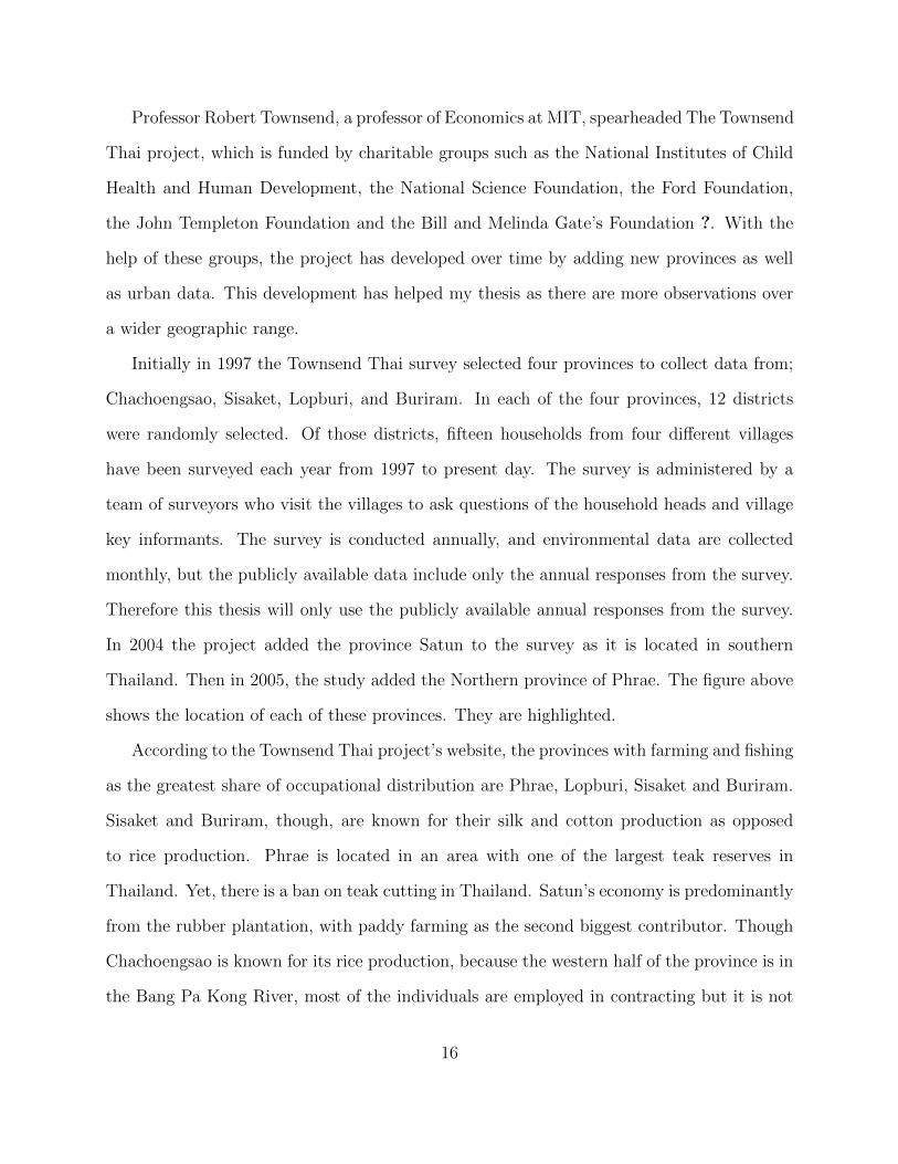
Figure 1: Study Area Provinces
This thesis uses data from the Townsend
Thai project. The Townsend Thai project
started in 1997 to study household responses
to shocks to their income and various policy
changes (National Bureau of Economic Re-
search, 1999). In 1998 Thailand experienced
a large shock to its economy from Asia’s fi-
nancial crisis which caused its economy to
contract by 10.5% (International Monetary
Fund, 2000). This spurred the government
to implement a set of programs to aid in the
re-growth of Thailand’s economy and assist
households that were experiencing shocks
to their income. The International Mone-
tary Fund also provided Thailand with over
US$17 billion of financial aid (International
Monetary Fund, 2012). As a result of the fi-
nancial crisis and policy changes, the Townsend Thai survey was formatted to measure house-
hold responses to the financial crisis and the effects of the policy changes. The Townsend
Thai project is panel data, meaning that it follows the same set of households from 1997 to
present day. The length of the time period is useful to researchers because we are better
able answer questions that we were unable to with the use of cross-sectional or time-series
data. More specifically, it makes it possible to control for unobservable time-invariant char-
acteristics of households.
15
Professor Robert Townsend, a professor of Economics at MIT, spearheaded The Townsend
Thai project, which is funded by charitable groups such as the National Institutes of Child
Health and Human Development, the National Science Foundation, the Ford Foundation,
the John Templeton Foundation and the Bill and Melinda Gate’s Foundation ?. With the
help of these groups, the project has developed over time by adding new provinces as well
as urban data. This development has helped my thesis as there are more observations over
a wider geographic range.
Initially in 1997 the Townsend Thai survey selected four provinces to collect data from;
Chachoengsao, Sisaket, Lopburi, and Buriram. In each of the four provinces, 12 districts
were randomly selected. Of those districts, fifteen households from four different villages
have been surveyed each year from 1997 to present day. The survey is administered by a
team of surveyors who visit the villages to ask questions of the household heads and village
key informants. The survey is conducted annually, and environmental data are collected
monthly, but the publicly available data include only the annual responses from the survey.
Therefore this thesis will only use the publicly available annual responses from the survey.
In 2004 the project added the province Satun to the survey as it is located in southern
Thailand. Then in 2005, the study added the Northern province of Phrae. The figure above
shows the location of each of these provinces. They are highlighted.
According to the Townsend Thai project’s website, the provinces with farming and fishing
as the greatest share of occupational distribution are Phrae, Lopburi, Sisaket and Buriram.
Sisaket and Buriram, though, are known for their silk and cotton production as opposed
to rice production. Phrae is located in an area with one of the largest teak reserves in
Thailand. Yet, there is a ban on teak cutting in Thailand. Satun’s economy is predominantly
from the rubber plantation, with paddy farming as the second biggest contributor. Though
Chachoengsao is known for its rice production, because the western half of the province is in
the Bang Pa Kong River, most of the individuals are employed in contracting but it is not
16

clear what type of contracting people are doing.
Table 1 gives major economic variables and environmental variables by province. From
the table, we see that all of the study provinces use the majority of their land for rice pro-
duction, with the exceptions of Phrae, Satun and Chachoengsao. Buriram and Sisaket have
the largest populations of the selected provinces while Satun and Phrae have the smallest
populations. The GDP per capita has a wide range from 34 thousand baht (Sisaket) to
285 thousand baht (Chachoengsao). While the provinces of Buriram and Sisaket have some
of the largest GDP’s relative to the other provinces, they have the lowest two GDP’s per
capita. They also have the largest rice production out of all of the provinces. It appears
that Buriram and Sisaket are the poorest of the selected provinces and among those most
dependent on agriculture. This implies that households from these provinces may be less
able to cope with shocks as well as more vulnerable to environmental shocks.
In terms of environmental variables, according to Table 1, Sisaket had the lowest number
of days of rainfall and the lowest temperature in 2010. That year, Buriram had the lowest
annual rainfall, Satun had the highest. Chachoengsao had the lowest average temperature
in 2010, while Lopburi had the highest. Those provinces with more extreme climates such as
Chachoengsao, Satun, Buriram and Lopburi will be more at risk to environmental shocks.
17

Tab
le1:
Eco
nom
ican
dE
nvir
onm
enta
lV
aria
ble
sby
Pro
vin
ce
Lop
buri
Chac
hoen
gsao
Buri
ram
Sis
aket
Sat
un
Phra
eT
otal
Eco
nom
icV
aria
ble
s
Pop
ula
tion
756,
127
679,
370
1,55
9,08
51,
452,
203
301,
467
458,
750
67,2
75,5
00
Per
cent
Mal
e50
.23
49.0
449
.950
49.8
648
.72
49.2
1
GD
P(2
009)
67,7
41m
n.
203,
011
mn.
62,4
72m
n.
52,5
78m
n.
25,9
84m
n.
23,3
75m
n.
9,04
1.6
bn.
GD
PP
erC
apit
a(2
009)
87,1
3728
5,29
038
,034
34,3
2690
,103
45,2
7813
5,14
4
Pct
.F
arm
Lan
d60
.56
27.8
959
.58
62.5
937
.82
16.2
41.0
3
Ric
eP
roduct
ion
(ton
)61
6,55
470
7,33
81,
185,
051
1,10
6,21
216
,856
163,
345
34,4
84,9
55
Ric
eY
ield
(kg.
/rai
)12
5812
4389
085
383
811
5110
58
Envir
onm
enta
lV
aria
ble
s
2010
Low
(Cel
sius)
13.3
15.6
12.9
2.0
21.9
13.6
NA
2010
Hig
h41
.839
.042
.241
.037
.043
.0N
A
2010
Ave
rage
28.8
27.3
27.5
28.0
27.9
27.5
NA
2010
Annual
Rai
nfa
ll(m
m)
1,08
5.4
1,71
3.6
591.
51,
071.
52,
026.
41,
007.
512
77.9
2010
Day
ofra
in14
614
513
499
185
127
155
Sta
tist
ics
taken
from
ThailandProvince
Data:2012-2013.
Alp
ha
Res
earc
h(2
013)
18

3.1 Migration in Thailand
Researchers have found that households in Thailand use migration as a way to reduce their
likelihood of entering poverty (Osaki, 2003; Jones and Pardthaisong, 1999; Curran and Saguy,
2006). The remittances from migrants become a new income source for the household. This
extra liquidity alleviates the pressure of making ends meet. According to the survey data,
both male and female migrants stay in Thailand when they migrate the majority of the time.
Another notable aspect of the locations of the migrants is in the early 2000’s one of
the top locations for all of the provinces is Bangkok, yet in the later years this changes
to a multitude of different destinations. Actually, in 2005, one of the top destinations for
migrants to travel to is Chaiyaphum. Chaiyaphum is located in the northeastern region of
Thailand. The province shares a border with Lopburi. The main economy of Chaiyaphum
comes from agriculture, but it is also well known for its silk industry. The other main
provinces that migrants are moving to are Tak, Pattani and Nonthaburi. It should be noted
that Nonthaburi, though a separate province, is part of the greater metropolitan Bangkok
area. In the early years of the dataset, of the top two destinations among migrants, both
genders were also staying within their province. This implies either that they might be
moving to larger cities in order to find different types of work or that they are moving to
different parts of the province but staying in agriculture in order to diversify the locations
household members are working. Knodel and Saengtienchai (2007) find that children who
migrate to an urban setting and remit improve the lives of their parents. But there is not
any information on if the migrant has moved from rural to urban in the survey data. Based
on the top occupations of migrants, which is discussed in more detail below, it could be
assumed that some migrants are staying in a rural setting but working as a farmer in a
different part of the province.
Researchers find that there are differences in gender roles with respect to migration in
Thailand. Mills (1997) recalls an interview with a female migrant who states that she decided
19

to migrate because she wanted to raise money for the family, but she was also inspired to
move by the beautiful clothes of her friend who was visiting from the city. In this example,
the migrant wants to improve her own lifestyle by moving to an urban setting while also
helping her family’s livelihood. Similarly, Marie et al. (2010) argue that, in North-eastern
Thailand, female migrants have fewer job opportunities and more pressure from their families
than their male counterparts.
This lack of opportunity and presence of gender roles cause the female migrants to follow
the decisions of the family more often than the male migrants who are more content with their
work situation and feel less pressure to come home when the family needs them. Sobieszczyk
(2000) also finds that male migrants had more opportunities to migrate abroad because they
had a stronger social network of individuals abroad who were willing to help them get
their first job. Their female counterparts were less likely to migrate abroad because they,
having a weaker social network, relied more on the overseas employers to arrange their first
jobs abroad. When considering the cultural effects of migration, Curran and Saguy (2001)
find that the gender of the migrant can impact the network that they construct through
migration. Yet at the same time the influence of the social networks feeds back and affects
the decisions of the migrant.
In fact, according to the survey data, female migrants send a greater amount of money
home more often than male migrants. Table 2 shows the average age of the migrant, times
money was sent to the household per year, and amount sent to the household per year based
on the gender of the migrant. The last two columns of the table give results from the t-test
of the means between the two genders. These results show that it is statistically significant
that female migrants send more money home more often. It is also the case, according to the
survey data, that more females migrate than males on average. This is possibly explained
by the counteracting effects of supply and demand. That is, according to the survey data,
women are more likely to migrate yet they have fewer opportunities than male migrants, as
20

stated above.
In terms of occupations, according to the survey data, male migrants work mostly as
either factory workers or rice farmers. Male migrants will also work as government officials
or policemen. Female migrants also work mostly as factory workers and rice farmers but
they might also take jobs in housework. One of the two notable trends over time from the
data is the consistency of both male and female migrants working as factory workers or rice
farmers. Something else that is notable is that the top two occupations and locations of
migrants from Buriram and Sisaket never change. They are always either factory workers or
rice farmers. Finally, the top two occupations in Satun and Phrae are much less consistent
than the top two occupations of the other provinces.
21

Tab
le2:
Des
crip
tive
Sta
tist
ics
ofM
ale
and
Fem
ale
Mig
rant
Rem
itta
nce
sSen
tA
nnual
ly
Money
Sent
toH
ouse
hold
from
Mig
rant
Mal
eF
emal
eT
test
mea
nsd
mea
nsd
bp
Age
34.6
89.
4734
9.15
.13
.24
Tim
esM
oney
Rec
eive
d5.
838.
047.
2112
.89
-1.1
8<
.001
Am
ount
Rec
eive
d10
110.
919
324.
1113
361.
6828
310.
89-3
235.
40<
.001
N66
6880
5828
190
Money
Sent
from
House
hold
toM
igra
nt
Mal
eF
emal
eT
test
mea
nsd
mea
nsd
bp
Age
28.8
88.
8627
.88
9.24
.13
.24
Tim
esM
oney
Sen
t4.
9313
.93
4.2
5.79
.04
.06
Am
ount
Sen
t21
138.
4242
384.
2725
420.
7178
858.
13-4
338.
5.3
5N
379
326
2819
0
The
Tab
legi
ves
the
aver
age
age,
mon
eyse
nt
toth
em
igra
nt,
and
mon
eyre
ceiv
edfr
omth
em
igra
nt
bas
edon
the
gender
ofth
em
igra
nt.
The
table
then
rep
orts
the
resu
lts
ofth
et-
test
ofdiff
eren
ces
ofth
ese
vari
able
s.
22

4 Key Variables
4.1 Dependent Variables
The number of migrants reported by each household is the main variable of interest. The
household survey considers migrants as members of the household even though they have
moved and are working in a new location for more than six months of the last twelve months.
Students studying in different parts of the country and members of the family that moved
to get married are not considered to be migrants. Household members are defined as, “all
the people who lived and ate in this house for at least 6 months out of the last 12 months
and children who are studying away from home and are supported by members of this
household.10” Those who have moved to get married are not considered members of the
household, even if the family member does not marry immediately. Each year, the household
reports how many migrants are working in other parts of the country, how much income the
migrant remits to the household ,and the gender of each migrant.
When broken down by year and province, the average number of female migrants is
higher than the average number of male migrants. After conducting t-tests of these means
broken down by province and year, there is either a significantly higher number of women
migrants or there is no significant difference between the average number of male and female
migrants per province and year. The two exceptions where there are more males than
females migrating are Buriram in 2006 and 2007. Other than that, we find that females
tend to migrate as often or more often than males. Table 3 gives descriptive statistics of
migrants broken by gender in the years 2001, 2005, and 2011. From this table, we see that
Chachoengsao, Lopburi, Buriram, and Sisaket tend to send out more migrants than Satun
and Phrae. For the most part, the average number of migrants appears to hover around two
10Seeing as migrants do not fit within the definition of a household member, the control for number ofhousehold members will be the number of migrants plus household members.
23

migrants per household with the exceptions of Satun and Phrae.
24

Tab
le3:
Des
crip
tive
Sta
tist
ics
ofM
igra
nts
All
Mig
rants
Mal
eM
igra
nts
Fem
ale
Mig
rants
Min
Med
ian
Mea
nM
axM
inM
edia
nM
ean
Max
Min
Med
ian
Mea
nM
ax
2001
Ch
ach
oen
gsao
02
2.32
120
22.
4411
01
1.63
10
Lop
bu
ri0
11.
9412
01
1.77
80
12.
0712
Bu
rira
m0
22.
4711
02.
52.
6811
02
2.36
10
Sis
aket
02
2.56
90
22.
89
02
2.17
7
Tot
al0
22.
3212
02
2.47
110
12.
0612
2005
Ch
ach
oen
gsao
01
2.05
110
11.
998
02
2.27
11
Lop
bu
ri0
11.
7411
01
1.61
110
12.
0911
Bu
rira
m0
22.
3711
02
2.33
100
22.
511
Sis
aket
02
2.35
100
22.
439
02
2.46
10
Sat
un
00
1.28
80
01.
367
00
1.81
8P
hra
e0
11.
115
01
1.24
50
11.
175
Tot
al0
11.
8811
01
1.97
110
22.
1411
2011
Ch
ach
oen
gsao
02
2.1
130
22.
19
02
2.16
9L
opb
uri
01
1.84
120
11.
7412
01
1.86
8B
uri
ram
02
2.39
110
22.
1411
02
2.55
11
Sis
aket
02
1.95
100
11.
869
02
1.86
7S
atu
n0
00.
687
00
0.47
30
00.
331
Ph
rae
00
0.63
60
00.
462
00
0.5
2
Tot
al0
11.
7813
01
1.8
120
21.
9811
Info
rmat
ion
take
nfr
omth
esu
rvey
dat
a.
25

4.2 Independent Variables
The explanatory variables that are of the most interest are the environmental shocks as well
as the loan and savings dummies. For the creation of the environmental shock variables, the
household survey includes a question asking the household head to report if this year, com-
pared to the prior year, was a good year for income. The exact question reads; “Comparing
this past year (June [year t-1] - May [ year t]) to the year before that (June [year t-2] - May
[year t-1]), which was the worst year for the household income?” The surveyor records one of
three different responses from the household head; this past year, the year before and income
exactly the same in both years. As a follow-up, the household head states why the year they
indicated would have been a particularly bad year for their income. Generally, the most
frequent responses from households is that their crop yield was affected by an environmental
shock such as flooding, drought or low crop yield. These responses are used to determine if
a household was affected by an external shock to their income, environmental or otherwise.
It should be noted that the original survey from 1997- 1999 included a different question
concerning a comparison of income across years which read, “Of the last 5 years, what was
the best year for household income?” Yet this time period in the dataset has been updated to
coincide with the aforementioned question and responses. This thesis will only be concerned
with the updated versions of the dataset for 1997 to 1999 because it parallels the responses
from the 2000- 2011 data.
I generated dummy variables for whether the household reported a shock to its income
in a particular year for each of the following different types of shock; flood, drought, low
crop yield11 and health/death. The health/ death dummy variable is a combination of if the
household head reported a health shock or a death in the family affecting household income.
The health/ death dummy variable will be used to compare with the environmental shock
11A large assumption that I make is that low crop yield implies that the household experienced an envi-ronmental shock. This may not always be the case.
26

variables to see if household responses are different in the case of covariate environmental
shocks versus idiosyncratic non-environmental shocks. Table 5 gives the number of reported
shocks from the years 2001, 2005 and 2011 by province. From the table, the highest re-
ported shocks are drought, flood, and low crop yield. The shock dummy variables were then
combined to create a categorical variable.12
Table 4: Tabulated Loans and Savings
Savings
No Yes Total
Loans No 1,339 2,809 4,148
Yes 2,446 9,430 11,876
Total 3,785 12,239 16,024
I then generated dummy variables for a
household’s use of either a loan or a sav-
ings account. Table 4 give the number of
households with loans, savings, both loans
and savings, and neither loans nor savings.
The table is pooled over time and across
provinces. A loan is defined as any money
or set of goods that anyone in the household
owed to, “ a commercial bank, the Bank for Agriculture and Agricultural Cooperatives
(BAAC), a PCG, a Rice Bank, the Agricultural Cooperative, a government agency, a mon-
eylender, a friend, a relative or any other individual or institution.” The surveyor also asked
if any household members had, “pawned/mortgaged land to anyone, sold your crops in ad-
vance, gotten goods on credit from a store owner or supplier of inputs.” The household
was defined to have savings if it had any savings in a Commercial Bank, the Agricultural
Cooperative, bank account at the BAAC, a production credit group account (PCG), gold,
jewelry, cash, rice in storage, and other crops in storage. There was an option for ‘other,’ but
it is unclear if the household would then include community/village banks. These dummies
are interacted with the shock categorical variable in order to determine if households use
migration as a coping mechanism when they have access to loans and savings and if those
decisions are different from households that do not have loans or savings.
12The following categories of this variable are 1- flood, 2- drought, 3- low crop yield, 4- health/death.
27

Table 5: Household Reported Shocks
Drought Flood Low Crop Yield Health/ Death Total
2001
Chachoengsao 13 1 35 6 55
Lopburi 38 12 17 6 73
Buriram 12 31 10 6 59
Sisaket 10 32 23 1 66
Total 73 76 85 19 253
2005
Chachoengsao 67 0 40 7 114
Lopburi 82 0 21 6 109
Buriram 23 2 18 9 52
Sisaket 86 0 22 6 114
Satun 9 0 38 2 49
Phrae 3 2 3 4 12
Total 270 4 142 34 450
2011
Chachoengsao 0 0 5 5 10
Lopburi 1 3 3 7 14
Buriram 36 5 0 4 45
Sisaket 1 1 0 1 3
Satun 0 0 0 1 1
Phrae 0 0 0 0 0
Total 38 9 8 18 73
28

4.3 Controls
There are a number of other explanatory variables that will be included in the model in order
to account for any potential bias in the results. These variables are meant to control for
any household characteristics that might affect household migration decisions. The controls
chosen for this thesis were influenced by Halliday (2012).
The first of these explanatory variables is the number of members in the household.
Again, households members are defined as, “all the people who lived and ate in this house
for at least 6 months out of the last 12 months and children who are studying away from
home and are supported by members of this household.” Table 6 gives the average number of
household members13 in each province in 2001, 2005, and 2011. From this table we see that
the average number of members for households in the study, by province, hovers around five
to six people. There doesn’t appear to be much variation over time for the average number
of household members per household.
The household surveys also report the age of the head of household and the highest grade
of education that the household head has completed. These two variables are included in the
model as they might also affect how the household makes decisions with respect to sending
out migrants under the framework of the New Economics of Labor Migration. Table 6 gives
descriptive statistics for the age of the household head and the number of years of education
for the household head for the years of 2001, 2005, and 2011. Here, the average age of the
household head hovers around 50 and doesn’t vary much over the years. The same goes for
the average years of education of the household head except in the case of Sisaket which
changes from seven years to nine years of education from 2005 to 2011. A set of dummy
variables are also included, which indicate the age range of the other household members.
13With migrants included in the calculation.
29

Tab
le6:
Des
crip
tive
Sta
tist
ics
ofC
ontr
olV
aria
ble
s
Hou
seh
old
Mem
ber
sA
geof
Hou
seh
old
Hea
dY
ears
ofS
chool
Min
Med
ian
Mea
nM
axM
inM
edia
nM
ean
Max
Min
Med
ian
Mea
nM
ax
2001
Ch
ach
oen
gsao
26
6.56
2030
52.5
52.4
911
10
76.
4322
Lop
bu
ri2
55.
9917
2853
51.9
986
07
7.26
22
Bu
rira
m3
66.
9816
3349
50.7
991
07
6.43
22
Sis
aket
37
7.15
2234
5454
.41
860
76.
9222
Tot
al3
66.
6722
3152
52.4
111
10
76.
7622
2005
Ch
ach
oen
gsao
26
6.05
1831
5351
.493
07
6.69
22
Lop
bu
ri4
55.
3822
4254
49.2
489
07
7.38
22
Bu
rira
m2
66.
1816
3150
48.3
897
07
6.58
22
Sis
aket
16
6.21
1928
5452
.26
930
77.
0722
Sat
un
25
5.75
1228
5153
.24
108
07
7.47
22
Ph
rae
24
4.5
1239
5451
.72
790
78.
5322
Tot
al2
65.
7222
3153
50.6
710
80
77.
1822
2011
Ch
ach
oen
gsao
16
6.09
1925
5656
.795
07
7.18
22
Lop
bu
ri1
55.
4714
2959
58.9
110
80
77.
8422
Bu
rira
m3
66.
3916
3554
53.9
584
07
7.23
22
Sis
aket
15
5.7
1423
54.5
54.4
593
07
8.11
22
Sat
un
25
5.12
1834
5151
.61
870
79.
3022
Ph
rae
24
3.94
941
.556
53.2
282
07
8.39
22
Tot
al2
55.
6319
3555
55.2
710
80
77.
8422
Info
rmat
ion
take
nfr
omsu
rvey
dat
a.
30

5 Methods
I estimate the number of migrants a household chooses to send out in response to household
reported shocks. The basic model I would estimate is
migrantsi = β0 + β1householdshocksi + ε. (1)
Yet there are issues with such a simple regression. First, with any simple regression of the
number of migrants in response to the household-reported shocks, there is the possibility of
endogeneity due to omitted variables. Endogeneity is a common issue in statistics. It occurs
when the error term, ε, is correlated with the explanatory variable causing the estimated
coefficient, β, to not be equal to the true coefficient, β. That is to say, not including controls
in the model causes us to assume that household reported shocks are the only thing affecting
the number of migrants and that no characteristics from the error term are correlated with
household reported shocks. This is not the case as there are many other variables that are
correlated with household shocks and will cause the household to make migration decisions.
For example, the number of members in the household is correlated with the number of
reports of health/death in the household, implying that if the number of household members
is not included in the model then the estimated coefficient will be biased. I must also control
for time because shocks and migration may both trend over time for unrelated reasons. In
order to mitigate this bias controls are included in the model.
migrantsit+1 = β0 + β1householdshocksit + β2yearit + β2+ncontrolsit + εit (2)
This model is known as a pooled ordinary least squares estimation. All of the households
from each year have been pooled together as one group and we assume that the coefficients
of this model are constant across both time and individual households. The issue with
31

this model is that there will still be some unobservable differences which remain in the
error term. It is possible that some of these unobservable characteristics are correlated
with the explanatory variables, leading to the problem of endogeneity. We can solve part
of this issue with the use of a fixed effects model that includes within estimators at the
household level. This will control for all time-invariant unobservable characteristics that
are correlated with the explanatory variables. But even then, we must assume that the
time-variant unobservable characteristics are either randomly distributed among households
or not correlated with the explanatory variables. Or we must assume that unobservable
characteristics are time-invariant.
A fixed effects model is estimated by subtracting the average value of each variable over
the time period of the panel from the linear unobserved effects model. In other words,
migrantsit −migrantsi = β1(householdshocksit − householdshocksi)+
β2(yearit − yeari) + β2+n(controlsit − controlsi) + (ai − ai) + (εit − εi) (3)
where for some variable xi,
xi =1
T
T∑t=1
xit.
With this calculation, the unobservable time-invariant individual effect, ai, is removed
from the model. The final fixed effects model becomes,
migrantsit = β0 + β1householdshocksit + β3controlsit + εit. (4)
With fixed effects, there are a number of assumptions that need to be satisfied in order
to ensure that the model is unbiased. First, each explanatory variable must change over
32

time with no perfectly linear relationship between explanatory variables. This implies that
explanatory variables like province or gender of the household head will not be included in
the model as they typically do not change over time.
Another important assumption is that the error term is homoscedastic and serially uncor-
related. That is to say, the error term for each observation cannot have any linear relationship
and they cannot be correlated over time. This assumption is satisfied because the model will
have robust standard errors. Robust standard errors correct for heterosckedasticity without
changing the coefficients of the model. When using robust standard errors they will be very
similar to FE standard errors, but they might be larger than the FE standard errors. This
may reduce the significance of some estimates, but the assumption of homoscedasticity is
fulfilled. If there is no issue with heteroskedasticity in the first place then the robust standard
errors will be equal to the original standard errors.
Finally and most importantly, the error term cannot be correlated with the explanatory
variables. As stated above, this is referred to as endogeneity and ultimately biases the es-
timates. I have already discussed some of the issues associated with endogeneity. First, if
controls are not included in the model and correlated with the error term then the estimates
will be biased. This was mitigated by including controls in the model. Second, there are
time-invariant characteristics that could be correlated with the explanatory variable. The
use of fixed effects controls for these time-invariant characteristics, but I can still not defini-
tively conclude that all of the unobserved time-variant characteristics that are correlated
with shocks are controlled for. It is the case, however, that the environmental shock vari-
ables are unlikely to be correlated with time-variant unobservable characteristics. That is,
environmental shocks are external to the household so the unobserved changes in character-
istics that influence migration are less likely to be correlated with shocks than with other
household level variables.
The model from equation four assumes that all households would do the same thing in the
33

case of an environmental shock. As pointed out in the literature review, this assumption is
false because households use many different coping mechanisms when confronted with shocks.
The literature review also indicated that the current research on migration and environmental
shocks does not take a detailed enough look at the households. It is important to understand
how these differences between households affect their decisions on migration.
Therefore, the model will be split into two models which show the differences between
households that have access to either loans or savings and those that do not. In the case
of savings, it is possible that the household is not actually saving in anticipation of an
environmental shock but, in any case, they still have access to extra liquidity in times that
they would need it. Conversely, we do not know exactly why a household has taken out
a loan. It is possible that this loan is being used to invest in capital or it is being used
to cope with difficult situations. Again, regardless of why it has this loan, the household
is in debt and therefore may feel larger constraints on its liquidity when it experiences an
environmental shock. This is because household members must cover their cost of living
while also paying off a loan. Another interpretation of households having loans should be
considered. Loans may be an indicator of a households access to credit. That is to say,
households that have loans are financially stable enough to take out more loans if they need
to. This implies that the causality could go the other way and the household with loans
would not send migrants away to cope with a shock. Here, it is best differentiate between
households that have either loans or savings and those that do not when we are trying to
understand the differences between these households. The two models are,
migrantsit+1 = β0 + β1savingsit−1 ∗ hhd shocksit + β2savingsit−1
+ β3hhd shocksit + β3+ncontrolsit + εit (5)
34

migrantsit+1 = β0 + β1loansit−1 ∗ hhd shocksit + β2loansit−1
+ β3hhd shocksit + β3+ncontrolsit + εit (6)
These models indicate the decisions that households with or without either loans or sav-
ings make when they are confronted with an environmental shock. Because there is an
interaction in the model all results will be expressed in terms of the marginal effects of a
given explanatory variable. With the marginal effects, β1 + β3 gives the change in migrants
from a household that has a loan/savings account and experiences an environmental shock
and β3 is the impact of an environmental shock on migration if the household does not have
savings/loans.14
Each of these three types of models will be broken down by male and female migrants to
determine the differences in migration decisions with respect to gender. They will also be
broken down by province. This will help determine if there is any difference in the decisions
that households in separate provinces make. Finally, time lags will be included in the model.
This means that for some year, t, I will measure the presence of a savings account in year t−1,
whether a shock occurs in year t, and the household migration decision in year t + 1. This
is meant to more accurately follow the course of events that might happen when households
experience a shock and make a migration decision, and minimize potential reverse causality.
That is to say, households will have a savings account or loan in the year before the shock
occurs. This may not be exactly in anticipation of the shock occurring but will influence how
the households makes coping decisions after the shock has occurred. The coping decision
that I am most concerned with is migration in the year after the shock has occurred. That
is, migration is an ex-post response to environmental shocks.
14ceteris paribus in all interpretations.
35

6 Results
6.1 Fixed Effects with No Interaction
As the research question looks for the effect of environmental shocks on migration, the
estimation starts with the most simple, yet reasonable, possible case. Table 7 shows a
fixed effects model of the impact of a shock in year t on all migrants in year t + 1. The
first column of this table gives the results of the provinces pooled together. This column
shows that there is no significant relationship between environmental shocks and migration
decisions. It is possible that these results are due to the differences in geographic location
and general characteristics of each of the different provinces. This implies that different
results might come from running the same regression on the separate provinces. The rest of
the table shows the same regression given each province. The province is listed at the top
of the column. When we break down the model by province we find almost no relationships
between environmental shocks and migration. The exception to this is drought and migration
in Lopburi. When households in Lopburi experience a drought they are likely to reduce the
number of migrants. It is still important to see if there are differences in these relationship
when migrants are broken into male and female that would not show up in the pooled model.
This is because many previous studies have shown the different migration decisions based
on the gender of the migrant (Damon and Wisniewski, 2014; Halliday, 2012).
Table 8 and Table 9 estimate the same relationship as Table 7, but break migrants down
by sex. The first column of each table shows results for all of the provinces pooled together.
Again, it is important to break the regressions down by each province in order to see if there
is a different relationship between environmental shocks and migration. These results show
that there is mainly no relationship, but where there is one the results show that households
with female migrants are more likely to send the migrant away when they report a shock
to their income. This is the case in Sisaket and Satun when households report low crop
36

yield. The relationship between drought and Lopburi is the same as when the migrants are
pooled together. There, the households decide to reduce the number of female migrants after
experiencing drought.
In the instance of male migrants we find a somewhat similar story to female migrants.
There is little to no relationship between environmental shocks and migration. When there
are relationships, male migrants come home when the household experiences an environmen-
tal shock. This is the case in Phrae when the household reports a flood and Chachoengsao
when the household experiences low crop yield. Despite the fact that these results are begin-
ning to show a relationship between environmental shocks and migrations, it is still important
to look at different cases. As pointed out in the literature review, different households may
make different decisions depending on the other coping mechanisms available to them and
their circumstances more generally. It is crucial that we allow for these differences when
modeling the relationships. The next two sets of results will include interactions with either
savings or loans in order to get a better idea of the types of households that make migration
decisions in response to environmental shocks and what kind of decisions they make.
37

Tab
le7:
Fix
edE
ffec
tson
All
Mig
rants
int+
1
(1)
(2)
(3)
(4)
(5)
(6)
(7)
All
Lop
buri
Bu
rira
mP
hra
eC
hac
hoen
gsao
Sis
ake
tS
atu
n
Nu
mb
erof
Mem
ber
s3.
6e-0
2∗1.
1e-0
22.
4e-0
23.
4e-0
27.
1e-0
21.
1e-
02
5.3
e-02
(1.6
e-02
)(3
.6e-
02)
(3.6
e-02
)(6
.6e-
02)
(4.2
e-02
)(3
.4e-
02)
(4.8
e-02)
Hh
dH
ead
Age
-3.4
e-03
-5.2
e-03
6.7e
-04
-3.7
e-02
∗-9
.4e-
032.3
e-03
-2.1
e-02
(3.5
e-03
)(6
.6e-
03)
(6.9
e-03
)(1
.7e-
02)
(9.8
e-03
)(6
.9e-
03)
(1.1
e-02)
Hh
dH
ead
Sch
ool
-1.9
e-02
1.3e
-03
-4.0
e-03
-9.7
e-02
∗∗-5
.1e-
03-5
.3e-
02
-5.5
e-02
(1.4
e-02
)(2
.5e-
02)
(3.7
e-02
)(3
.6e-
02)
(3.1
e-02
)(3
.2e-
02)
(3.7
e-02)
Far
mer
-2.6
e-02
-7.3
e-03
-1.2
e-01
1.3e
-01
1.7e
-02
8.1
e-02
-2.8
e-01
(6.0
e-02
)(1
.0e-
01)
(1.4
e-01
)(1
.4e-
01)
(1.3
e-01
)(1
.6e-
01)
(1.8
e-01)
Flo
od
1.6e
-01
-8.9
e-02
2.1e
-01
7.3e
-02
-2.7
e-01
2.8
e-01
(1.4
e-01
)(2
.9e-
01)
(2.3
e-01
)(5
.9e-
01)
(6.1
e-01
)(2
.3e-
01)
Dro
ugh
t-1
.1e-
01-2
.5e-
01∗
-1.9
e-01
1.3e
-01
-7.1
e-02
8.7
e-02
-5.6
e-01
(7.3
e-02
)(1
.2e-
01)
(1.4
e-01
)(4
.4e-
01)
(2.0
e-01
)(1
.4e-
01)
(6.4
e-01)
Low
Yie
ld3.
0e-0
3-9
.2e-
02-1
.2e-
01-1
.8e-
03-2
.6e-
013.9
e-01
2.6
e-01
(8.5
e-02
)(1
.6e-
01)
(2.2
e-01
)(2
.8e-
01)
(1.5
e-01
)(2
.3e-
01)
(1.7
e-01)
Hea
lth
/Dea
th2.
4e-0
2-1
.7e-
012.
6e-0
13.
6e-0
1-1
.8e-
018.0
e-01
-3.0
e-01
(1.4
e-01
)(2
.3e-
01)
(3.3
e-01
)(3
.2e-
01)
(2.8
e-01
)(5
.1e-
01)
(3.3
e-01)
Con
stan
t2.
2e+
00∗∗
∗2.
1e+
00∗∗
∗2.
4e+
00∗∗
∗3.
6e+
00∗∗
2.3e
+00
∗∗∗
2.4e
+00∗∗
∗2.4
e+00∗∗
(2.6
e-01
)(5
.2e-
01)
(5.3
e-01
)(1
.2e+
00)
(6.1
e-01
)(5
.5e-
01)
(8.7
e-01)
N12
053
2583
2614
693
2596
2622
830
R2
0.00
110.
0019
0.00
260.
0142
0.00
270.0
065
0.0
164
r2a
3.9e
-04
-1.2
e-03
-4.9
e-04
2.6e
-03
-4.1
e-04
3.4
e-03
8.0
e-03
sein
par
enth
eses
∗p<
0.05
,∗∗
p<
0.01
,∗∗
∗p<
0.0
01
38

Tab
le8:
Fix
edE
ffec
tson
Fem
ale
Mig
rants
int+
1
(1)
(2)
(3)
(4)
(5)
(6)
(7)
All
Lop
bu
riB
uri
ram
Ph
rae
Ch
ach
oen
gsao
Sis
ake
tS
atu
n
Nu
mb
erof
Mem
ber
s1.
2e-0
22.
9e-0
2-6
.2e-
03-4
.9e-
034.
5e-0
2-2
.9e-
02
5.7
e-02∗
(1.0
e-02
)(2
.3e-
02)
(2.0
e-02
)(4
.0e-
02)
(2.4
e-02
)(2
.2e-
02)
(2.6
e-02)
Hh
dH
ead
Age
8.8e
-04
-3.1
e-03
7.3e
-04
-2.1
e-02
-6.9
e-03
-1.1
e-03
-1.1
e-02
(2.1
e-03
)(5
.1e-
03)
(4.2
e-03
)(1
.1e-
02)
(5.7
e-03
)(4
.1e-
03)
(6.3
e-03)
Hh
dH
ead
Sch
ool
-1.3
e-02
1.5e
-02
6.2e
-03
-7.3
e-02
∗∗5.
8e-0
3-4
.1e-
02∗
-1.5
e-02
(8.3
e-03
)(2
.1e-
02)
(2.1
e-02
)(2
.4e-
02)
(1.9
e-02
)(1
.8e-
02)
(2.2
e-02)
Far
mer
-3.9
e-02
6.6e
-02
-5.5
e-02
4.6e
-02
-8.9
e-03
1.1e-
01
-2.2
e-01
(3.5
e-02
)(6
.9e-
02)
(8.2
e-02
)(1
.0e-
01)
(7.4
e-02
)(9
.8e-
02)
(1.2
e-01)
Flo
od
9.3e
-02
5.7e
-02
3.6e
-02
2.0e
-01
1.3e
-01
4.0e-
02
(9.1
e-02
)(2
.0e-
01)
(1.2
e-01
)(6
.5e-
01)
(4.4
e-01
)(1
.5e-
01)
Dro
ugh
t7.
7e-0
3-2
.0e-
01∗
-7.9
e-02
-6.4
e-02
-8.3
e-02
-5.3
e-03
-2.8
e-01
(4.2
e-02
)(8
.6e-
02)
(7.8
e-02
)(2
.1e-
01)
(1.2
e-01
)(8
.2e-
02)
(3.8
e-01)
Low
Yie
ld-3
.4e-
02-8
.9e-
03-7
.6e-
021.
0e-0
1-8
.4e-
022.
9e-
01∗
2.7
e-01∗
(4.7
e-02
)(1
.2e-
01)
(1.3
e-01
)(9
.4e-
02)
(1.0
e-01
)(1
.4e-
01)
(1.2
e-01)
Hea
lth
/Dea
th7.
3e-0
2-1
.5e-
011.
3e-0
1-1
.1e-
01-9
.3e-
022.
2e-
01
-1.7
e-01
(8.1
e-02
)(1
.3e-
01)
(1.9
e-01
)(2
.7e-
01)
(1.5
e-01
)(2
.7e-
01)
(2.1
e-01)
Con
stan
t9.
4e-0
1∗∗∗
8.6e
-01∗
1.2e
+00
∗∗∗
2.2e
+00
∗∗1.
2e+
00∗∗
∗1.
6e+
00∗∗
∗9.9
e-01
(1.5
e-01
)(4
.0e-
01)
(3.2
e-01
)(8
.0e-
01)
(3.6
e-01
)(3
.1e-
01)
(5.1
e-01)
N12
053
2583
2614
693
2596
2622
830
R2
0.00
120.
0038
0.00
120.
0113
0.00
230.0
054
0.0
236
r2a
5.0e
-04
7.2e
-04
-1.8
e-03
-3.1
e-04
-7.5
e-04
2.4e-
03
1.5
e-02
sein
par
enth
eses
∗p<
0.05
,∗∗
p<
0.0
1,∗∗
∗p<
0.001
39

Tab
le9:
Fix
edE
ffec
tson
Mal
eM
igra
nts
int+
1
(1)
(2)
(3)
(4)
(5)
(6)
(7)
All
Lop
buri
Bu
rira
mP
hra
eC
hac
hoen
gsao
Sis
ake
tS
atu
n
Nu
mb
erof
Mem
ber
s1.
5e-0
2-2
.3e-
024.
7e-0
39.
8e-0
33.
0e-0
22.
5e-
02
-2.4
e-03
(9.9
e-03
)(2
.3e-
02)
(2.1
e-02
)(4
.2e-
02)
(2.4
e-02
)(2
.0e-
02)
(3.0
e-02)
Hh
dH
ead
Age
-3.5
e-03
-1.8
e-03
2.4e
-03
-2.4
e-02
∗-3
.6e-
035.
7e-
03
-1.0
e-02
(2.1
e-03
)(3
.7e-
03)
(4.1
e-03
)(1
.1e-
02)
(5.2
e-03
)(4
.2e-
03)
(6.1
e-03)
Hh
dH
ead
Sch
ool
-4.8
e-03
-9.9
e-03
-1.7
e-02
-3.7
e-02
∗-1
.1e-
02-8
.4e-
03
-3.8
e-02
(8.8
e-03
)(1
.4e-
02)
(2.1
e-02
)(1
.7e-
02)
(1.5
e-02
)(2
.2e-
02)
(2.0
e-02)
Far
mer
2.8e
-03
-7.6
e-02
-9.3
e-02
6.4e
-02
2.4e
-02
-1.7
e-02
-1.1
e-01
(3.7
e-02
)(6
.2e-
02)
(8.4
e-02
)(8
.7e-
02)
(7.1
e-02
)(9
.6e-
02)
(9.5
e-02)
Flo
od
4.4e
-02
-1.4
e-01
2.1e
-01
-4.0
e-01
∗∗-4
.7e-
011.
4e-
01
(8.2
e-02
)(1
.7e-
01)
(1.5
e-01
)(1
.4e-
01)
(2.6
e-01
)(1
.4e-
01)
Dro
ugh
t-8
.6e-
02∗
-2.7
e-02
-4.2
e-02
2.3e
-01
4.1e
-03
1.0
e-01
-2.2
e-01
(4.3
e-02
)(6
.3e-
02)
(8.2
e-02
)(2
.8e-
01)
(1.1
e-01
)(8
.5e-
02)
(2.8
e-01)
Low
Yie
ld5.
5e-0
2-8
.9e-
021.
5e-0
24.
0e-0
2-1
.8e-
01∗
7.9
e-02
6.6
e-02
(5.4
e-02
)(9
.9e-
02)
(1.2
e-01
)(2
.3e-
01)
(8.0
e-02
)(1
.3e-
01)
(8.6
e-02)
Hea
lth
/Dea
th-4
.1e-
022.
2e-0
31.
8e-0
14.
4e-0
1-8
.9e-
024.1
e-01
3.7
e-04
(7.8
e-02
)(1
.3e-
01)
(2.0
e-01
)(2
.3e-
01)
(1.5
e-01
)(3
.5e-
01)
(1.5
e-01)
Con
stan
t1.
2e+
00∗∗
∗1.
2e+
00∗∗
∗1.
2e+
00∗∗
∗2.
0e+
00∗∗
1.1e
+00
∗∗∗
6.9e-
01∗
1.3
e+00∗∗
(1.6
e-01
)(3
.0e-
01)
(3.1
e-01
)(7
.5e-
01)
(3.1
e-01
)(3
.3e-
01)
(4.5
e-01)
N12
053
2583
2614
693
2596
2622
830
R2
0.00
090.
0022
0.00
310.
0206
0.00
360.
0062
0.0
109
r2a
2.4e
-04
-9.4
e-04
6.1e
-05
9.1e
-03
4.7e
-04
3.2e-
03
2.5
e-03
sein
par
enth
eses
∗p<
0.05
,∗∗
p<
0.01
,∗∗
∗p<
0.0
01
40

6.2 Fixed Effects with Savings Interaction
As in the previous section, I consider the simplest case with the interaction and then break
the results down further. All of the results given in Tables 10, 11, and 12 show marginal
effects of shocks on migration for households with and without savings rather than the raw
coefficients. In these tables, the top four rows give the marginal effects of environmental
shocks on migration for households that do not have savings. Then rows six through nine
give the marginal effects of shocks on migration in the case of households that do have
savings.
In Table 10, the first column gives the results when all of the provinces are pooled together
for all migrants. As before, there is no significant relationship between environmental shocks
and migration in this regression. The next six columns give the results of the same regression,
but all of the provinces are separated. Again, there is little to no significant relationship
between environmental shocks and household decisions to migrate. However, when male
and female migrants are separated, I observe differing impacts of environmental shocks on
migration.
Table 11 reports the impacts of environmental shocks in year t on male migrants in year
t+ 1 for households with and without savings. When all provinces are pooled together, the
results indicate that where there is significance, namely in the cases of drought and ill health
or death in the household, households that have savings and experience a shock to their
income will reduce the number of migrants. This regression also shows that households that
do not have savings and experience a shock will send migrants away. Breaking down the
regression by province shows where households are making these migration decisions as well
as under what circumstances they are making these decisions. When the regression is broken
down by province the results are similar in that, where there is a significant relationship, the
household that experiences a shock and has a savings will have migrants come home while
households that experience a shock but do not have a savings will send migrants away. The
41

only exceptions in this set of results are when the household experiences a flood in Lopburi
and Phrae with no savings. In this case, the households will have migrants come home.
Table 12 gives the results for female migrants when the household experiences a shock
interacted with the savings dummy. When all of the provinces are pooled together as one in
the first column the results indicate that there is no migration response to flood or low yield,
but in the case of drought, households that experience a shock to their income and do not
have a savings account will send migrants away. Households that experience a shock to their
income and have a savings account will have the migrants come home. This is similar in the
case of ill health/death. When the regression is run by province, the results are similar to
those of the pooled provinces in Sisaket and Buriram. Similar to the case of male migrants,
when a household does not experience a shock and has a savings account then they will send
migrants away.
When comparing Tables 11 and 12, a pattern emerges. When the household experiences
drought, it will both have a migrant come home or send migrants away depending on if it
has savings or not. Generally there is no relationship between either flood, low crop yield, or
drought and migration. There is a somewhat similar relationship to drought in the case of
health/death. Based on the gender of the migrant, this pattern appears in different provinces.
In other words, this pattern occurs in Chachoengsao and Sisaket for male migrants while,
for female migrants the pattern occurs in Buriram. The pattern also appears in Sisaket for
female migrants, but only in the case of drought.
42

Tab
le10
:Sav
ings
Hou
sehol
dF
Ew
ith
Bot
hla
gsan
dA
llM
igra
nts
(1)
(2)
(3)
(4)
(5)
(6)
(7)
All
Chac
hoen
gsao
Lop
buri
Buri
ram
Sis
aket
Sat
un
Phra
eF
lood
0.52
6-0
.027
0-0
.658
0.58
41.
409
0.31
4(0
.488
)(1
.582
)(0
.453
)(0
.687
)(1
.150
)(0
.669
)
Dro
ugh
t0.
0581
0.60
1-0
.246
0.02
250.
249
-0.3
810.
167
(0.1
29)
(0.4
54)
(0.1
98)
(0.2
78)
(0.2
37)
(0.5
26)
(0.4
17)
Low
Cro
pY
ield
-0.1
75-0
.687
0.01
83-0
.487
0.04
17-0
.620
1.25
7(0
.244
)(0
.483
)(0
.436
)(0
.556
)(0
.434
)(0
.811
)(1
.063
)
Hea
lth/
Dea
th0.
297
0.30
2-0
.032
40.
470
0.79
5-0
.441
0.00
554
(0.1
71)
(0.3
27)
(0.4
82)
(0.3
64)
(0.4
09)
(0.4
30)
(0.4
05)
Sav
ings
-0.0
512
0.14
6-0
.092
20.
0038
4-0
.088
5-0
.355
-0.2
92∗
(0.0
671)
(0.1
46)
(0.1
27)
(0.1
65)
(0.1
59)
(0.2
75)
(0.1
39)
Sav
e*F
lood
-0.3
48-0
.235
0.56
6-0
.331
-1.2
38(0
.501
)(1
.701
)(0
.538
)(0
.706
)(1
.163
)
Sav
e*D
rough
t-0
.155
-0.6
14-0
.020
8-0
.229
-0.1
90(0
.140
)(0
.486
)(0
.212
)(0
.289
)(0
.276
)
Sav
e*L
owY
ield
0.19
60.
362
-0.0
814
0.68
51.
005
0.28
3-0
.721
(0.2
82)
(0.5
82)
(0.4
82)
(0.6
75)
(0.8
24)
(0.8
53)
(1.1
03)
Sav
e*H
ealt
h/
Dea
th-0
.303
-0.5
70-0
.056
4-0
.644
-0.4
820.
734
0.24
7(0
.187
)(0
.365
)(0
.494
)(0
.416
)(0
.429
)(0
.477
)(0
.413
)N
1769
538
6540
1839
2338
9897
888
7
sein
par
enth
eses
∗p<
0.05
,∗∗
p<
0.01
,∗∗
∗p<
0.0
01
43

Tab
le11
:Sav
ings
Hou
sehol
dF
Ew
ith
Bot
hla
gsan
dM
ale
Mig
rants
(1)
(2)
(3)
(4)
(5)
(6)
(7)
All
Chac
hoen
gsao
Lop
buri
Buri
ram
Sis
aket
Sat
un
Phra
eF
lood
0.54
10.
637
-0.5
50∗∗
0.77
50.
691
-0.2
48∗
(0.2
91)
(0.8
87)
(0.1
95)
(0.4
46)
(0.5
80)
(0.1
20)
Dro
ugh
t0.
344∗
∗∗0.
726∗
0.18
40.
299
0.51
4∗∗∗
-0.1
700.
302
(0.0
808)
(0.3
01)
(0.1
12)
(0.1
74)
(0.1
50)
(0.2
10)
(0.2
57)
Low
Cro
pY
ield
0.33
5∗-0
.165
0.58
80.
188
0.62
9∗∗
-0.5
580.
538
(0.1
55)
(0.2
11)
(0.3
10)
(0.2
87)
(0.2
39)
(0.3
56)
(0.9
82)
Hea
lth/
Dea
th0.
424∗
∗∗0.
507∗
∗0.
328
0.30
10.
959∗
∗∗-0
.212
-0.1
87(0
.095
2)(0
.184
)(0
.278
)(0
.194
)(0
.250
)(0
.215
)(0
.321
)
Sav
ings
0.07
160.
194∗
0.04
950.
0639
0.11
3-0
.197
-0.1
23(0
.037
6)(0
.077
2)(0
.063
3)(0
.102
)(0
.094
5)(0
.147
)(0
.091
0)
Sav
e*F
lood
-0.4
29-1
.092
0.45
6-0
.558
-0.6
04(0
.294
)(0
.922
)(0
.256
)(0
.445
)(0
.595
)
Sav
e*D
rough
t-0
.321
∗∗∗
-0.7
13∗
-0.2
29-0
.365
∗-0
.390
∗
(0.0
890)
(0.3
29)
(0.1
22)
(0.1
85)
(0.1
74)
Sav
e*L
owY
ield
-0.2
870.
0475
-0.5
53-0
.133
-0.1
790.
469
0.05
83(0
.170
)(0
.261
)(0
.313
)(0
.364
)(0
.493
)(0
.372
)(1
.024
)
Sav
e*H
ealt
hD
eath
-0.4
68∗∗
∗-0
.710
∗∗∗
-0.4
31-0
.282
-0.8
99∗∗
0.27
50.
345
(0.1
05)
(0.2
02)
(0.2
87)
(0.2
26)
(0.2
79)
(0.2
45)
(0.4
03)
N17
931
3918
4080
3980
3962
978
887
sein
par
enth
eses
∗p<
0.0
5,∗∗
p<
0.01
,∗∗
∗p<
0.001
44

Tab
le12
:Sav
ings
Hou
sehol
dF
Ew
ith
Bot
hla
gsan
dF
emal
eM
igra
nts
(1)
(2)
(3)
(4)
(5)
(6)
(7)
All
Chac
hoen
gsao
Lop
buri
Buri
ram
Sis
aket
Sat
un
Phra
eF
lood
0.50
50.
631
0.06
670.
372
1.37
0∗0.
336
(0.2
91)
(0.5
40)
(0.4
44)
(0.3
74)
(0.6
83)
(0.6
83)
Dro
ugh
t0.
307∗
∗∗0.
436
0.10
90.
323∗
0.46
6∗∗∗
-0.1
51-0
.083
5(0
.078
6)(0
.257
)(0
.137
)(0
.163
)(0
.140
)(0
.329
)(0
.216
)
Low
Cro
pY
ield
0.04
820.
162
-0.1
57-0
.162
0.29
4-0
.073
00.
211
(0.1
28)
(0.2
98)
(0.1
94)
(0.3
02)
(0.3
07)
(0.4
80)
(0.2
91)
Hea
lth/
Dea
th0.
445∗
∗∗0.
338
0.25
90.
821∗
∗∗0.
459
-0.2
510.
234
(0.1
09)
(0.2
03)
(0.2
71)
(0.2
24)
(0.2
82)
(0.2
83)
(0.3
33)
Sav
ings
0.13
1∗∗
0.19
7∗0.
0820
0.25
7∗∗
0.12
6-0
.171
-0.1
27(0
.040
6)(0
.090
7)(0
.079
8)(0
.092
3)(0
.094
1)(0
.154
)(0
.096
8)
Sav
e*F
lood
-0.4
45-0
.483
-0.0
512
-0.2
85-1
.417
∗
(0.3
02)
(0.6
94)
(0.4
90)
(0.3
94)
(0.6
91)
Sav
e*D
rough
t-0
.381
∗∗∗
-0.4
98-0
.281
-0.4
26∗
-0.4
84∗∗
(0.0
850)
(0.2
78)
(0.1
51)
(0.1
70)
(0.1
59)
Sav
e*L
owY
ield
-0.0
504
-0.3
020.
119
0.32
70.
0676
-0.0
510
-0.2
70(0
.157
)(0
.345
)(0
.249
)(0
.391
)(0
.487
)(0
.513
)(0
.385
)
Sav
e*H
ealt
h/
Dea
th-0
.374
∗∗-0
.403
-0.2
39-0
.952
∗∗∗
-0.1
630.
557
-0.0
359
(0.1
19)
(0.2
32)
(0.2
84)
(0.2
49)
(0.2
92)
(0.3
15)
(0.3
25)
N17
931
3918
4080
3980
3962
978
887
sein
par
enth
eses
∗p<
0.05
,∗∗
p<
0.01
,∗∗
∗p<
0.001
45

6.3 Fixed Effects with Loan Interaction
The loan dummy variable was then interacted with the shock categorical variable in order
to get a better idea of the differences in decisions made by households that have loans and
households that do not have loans. Again, all of the results listed in the following tables
are of the marginal effects of shocks on migration for households with and without loans.
According to Table 15, when all of the migrants are pooled together and the provinces
are pooled, there is no relationship. When the provinces are separated, there is mainly no
relationship between environmental shocks and migration. But where there is a relationship,
the results indicate that households that experience a shock to their income and do not have
a loan will choose to have migrants come home, while households that experience a shock
to their income and have a loan will send migrants away. Notice that for particular shocks,
low crop yield in Lopburi and Buriram and drought in Sisaket, the results will switch signs
depending on whether or not the household has a loan. Again, the results are more revealing
of household decisions when the regressions are separated by gender.
Table 14 gives the results for the impact of environmental disasters interacted with loans
on male migration. The first column shows that when the provinces are pooled together,
there is no relationship between environmental shocks and male migrants. When the models
become more detailed by breaking them up into provinces we find that if there is any rela-
tionship, households will have a migrant come home when they experience an environmental
shock and do not have a loan. Conversely, households will send migrants away when they
experience a shock to their income and have a loan. This relationship is in the case of low
crop yield in Lopburi and Buriram. There is also some evidence of a similar relationship
between drought and migration.
Female migrants yield similar results to male migrants with the loan interaction. This
means that in the cases when the household experiences a shock to their income and does
not have a loan, they are going to have migrants come home while when the household does
46

have a loan and experiences a shock, they will send migrants away. The exception in this
case is households in Lopburi that experience a flood. In this instance the households will
send migrants out when they do not have a loan and have migrants come home when they
do have a loan. Again, there is no relationship between households that did not experience
a shock to their income and have a loan and their decisions as to whether to bring migrants
home or send them out.
In the case of loans, as opposed to savings, the results switch signs for low crop yield
in the case of both male and female migrants. That is to say, when households with a
loan experience an environmental shock, they will increase the number of migrants, while
households without loans that experience shocks will reduce the number of migrants. This
relationship occurs in Lopburi when households experience low crop yield for both male and
female migrants and in Buriram when households experience low crop yield for just male
migrants. For female migrants only, there is a sign switch for two provinces in the case of
flood. These provinces are Lopburi and Sisaket. But, in the case of Lopburi, households will
increase the number of migrants when they experience a flood and do not have a loan, while
households with loans that experience flooding with reduce the number of migrants.
47

Tab
le13
:L
oan
Hou
sehol
dF
Ew
ith
Bot
hla
gsan
dA
llM
igra
nts
(1)
(2)
(3)
(4)
(5)
(6)
(7)
All
Chac
hoen
gsao
Lop
buri
Buri
ram
Sis
aket
Sat
un
Phra
eF
lood
0.15
4-0
.129
1.00
30.
448
-0.5
13-0
.101
(0.4
36)
(1.4
40)
(0.9
73)
(0.8
52)
(0.5
16)
(0.3
92)
Dro
ugh
t-0
.284
-0.0
595
-0.0
169
-0.1
84-0
.661
∗-0
.561
∗∗∗
0.13
9(0
.171
)(0
.392
)(0
.405
)(0
.338
)(0
.313
)(0
.132
)(0
.113
)
Low
crop
Yie
ld-0
.278
0.33
5-1
.480
∗∗∗
-1.3
56∗∗
∗1.
132
-0.5
090.
347
(0.3
74)
(0.9
96)
(0.3
16)
(0.2
52)
(1.1
24)
(0.3
47)
(0.5
47)
Hea
lth/
Dea
th-0
.075
3-0
.530
-0.2
970.
762
0.04
620.
320
-0.5
29(0
.173
)(0
.295
)(0
.439
)(0
.614
)(0
.462
)(0
.321
)(0
.368
)
Loa
n0.
0492
-0.0
0162
0.09
300.
223
-0.0
744
0.11
5-0
.011
0(0
.063
3)(0
.132
)(0
.137
)(0
.209
)(0
.146
)(0
.163
)(0
.127
)
Loa
n*F
lood
0.02
00-0
.239
-1.2
43-0
.230
0.83
80.
519
(0.4
50)
(1.6
17)
(1.0
03)
(0.8
59)
(0.5
74)
(0.8
91)
Loa
n*D
rough
t0.
190
-0.0
375
-0.3
05-0
.020
90.
874∗
∗0.
195
-0.0
511
(0.1
84)
(0.4
36)
(0.4
26)
(0.3
63)
(0.3
37)
(0.6
62)
(0.5
46)
Loa
n*L
owY
ield
0.34
1-0
.840
1.59
5∗∗∗
1.70
0∗∗∗
-0.1
38-0
.167
0.21
2(0
.419
)(1
.087
)(0
.430
)(0
.457
)(1
.380
)(0
.618
)(0
.734
)
Loa
n*H
ealt
h/
Dea
th0.
0437
0.34
00.
199
-1.0
900.
339
-0.1
890.
657
(0.1
97)
(0.3
23)
(0.4
86)
(0.6
91)
(0.5
13)
(0.4
19)
(0.4
83)
N11
167
2427
2316
2414
2445
806
650
sein
par
enth
eses
∗p<
0.05
,∗∗
p<
0.01
,∗∗
∗p<
0.0
01
48

Tab
le14
:L
oan
Hou
sehol
dF
Ew
ith
Bot
hla
gsan
dM
ale
Mig
rants
(1)
(2)
(3)
(4)
(5)
(6)
(7)
All
Chac
hoen
gsao
Lop
buri
Buri
ram
Sis
aket
Sat
un
Phra
eF
lood
0.06
75-0
.790
-0.2
670.
280
0.23
1-0
.435
∗
(0.2
62)
(0.6
46)
(0.4
10)
(0.5
30)
(0.3
88)
(0.2
06)
Dro
ugh
t-0
.100
-0.0
0810
0.11
9-0
.144
-0.2
50-0
.240
∗∗0.
581∗
∗∗
(0.0
920)
(0.2
04)
(0.2
20)
(0.1
77)
(0.1
73)
(0.0
819)
(0.1
20)
Low
Cro
pY
ield
-0.0
802
-0.0
988
-0.6
07∗∗
∗-0
.931
∗∗∗
0.80
1-0
.091
20.
750
(0.2
26)
(0.4
90)
(0.1
79)
(0.1
51)
(0.9
09)
(0.1
34)
(0.6
04)
Hea
lth/
Dea
th-0
.107
-0.3
83∗∗
-0.3
030.
633
-0.1
620.
152
-0.4
36(0
.087
1)(0
.132
)(0
.172
)(0
.324
)(0
.298
)(0
.162
)(0
.314
)
Loa
n0.
0448
0.01
980.
0528
0.14
2-0
.007
610.
110
-0.0
133
(0.0
348)
(0.0
733)
(0.0
718)
(0.1
16)
(0.0
818)
(0.0
831)
(0.0
688)
Loa
n*F
lood
0.03
120.
351
0.22
4-0
.091
7-0
.129
0.30
0(0
.276
)(0
.706
)(0
.446
)(0
.543
)(0
.422
)(0
.234
)
Loa
n*D
rough
t0.
110
-0.0
100
-0.2
070.
102
0.40
7∗0.
0381
-0.4
82(0
.102
)(0
.232
)(0
.234
)(0
.193
)(0
.198
)(0
.296
)(0
.365
)
Loa
n*L
owY
ield
0.15
2-0
.069
20.
740∗
∗1.
090∗
∗∗-0
.616
-0.1
47-0
.309
(0.2
48)
(0.5
23)
(0.2
65)
(0.2
76)
(1.0
12)
(0.2
58)
(0.6
63)
Loa
n*H
ealt
h/
Dea
th0.
0532
0.23
70.
206
-0.7
030.
222
-0.2
080.
631
(0.1
03)
(0.1
65)
(0.1
89)
(0.3
68)
(0.3
28)
(0.2
15)
(0.4
10)
N11
167
2427
2316
2414
2445
806
650
sein
par
enth
eses
∗p<
0.0
5,∗∗
p<
0.01
,∗∗
∗p<
0.001
49

Tab
le15
:L
oan
Hou
sehol
dF
Ew
ith
Bot
hla
gsan
dF
emal
eM
igra
nts
(1)
(2)
(3)
(4)
(5)
(6)
(7)
All
Chac
hoen
gsao
Lop
buri
Buri
ram
Sis
aket
Sat
un
Phra
eF
lood
0.16
70.
778
1.33
0∗0.
290
-0.5
97∗
-0.4
34(0
.259
)(0
.796
)(0
.606
)(0
.449
)(0
.272
)(0
.253
)
Dro
ugh
t-0
.151
-0.0
630
-0.1
590.
112
-0.4
21∗
-0.2
46∗∗
-0.2
68∗∗
∗
(0.1
08)
(0.2
24)
(0.2
40)
(0.2
29)
(0.2
03)
(0.0
911)
(0.0
749)
Low
Cro
pY
ield
-0.1
830.
388
-0.8
28∗∗
∗-0
.179
0.13
3-0
.229
-0.4
11∗
(0.1
82)
(0.5
13)
(0.2
11)
(0.1
52)
(0.3
16)
(0.2
62)
(0.1
88)
Hea
lth/
Dea
th0.
0593
-0.2
300.
0622
0.24
40.
293
0.28
0-0
.032
7(0
.113
)(0
.192
)(0
.335
)(0
.376
)(0
.285
)(0
.204
)(0
.086
9)
Loa
n0.
0211
-0.0
233
0.05
230.
146
-0.0
641
0.04
860.
0407
(0.0
391)
(0.0
821)
(0.0
857)
(0.1
21)
(0.0
926)
(0.0
969)
(0.0
778)
Loa
n*F
lood
-0.1
43-0
.808
-1.5
36∗
-0.2
450.
667∗
0.97
8(0
.266
)(0
.966
)(0
.631
)(0
.452
)(0
.313
)(0
.799
)
Loa
n*D
rough
t0.
0673
-0.0
400
-0.0
628
-0.2
260.
481∗
0.12
10.
248
(0.1
16)
(0.2
60)
(0.2
53)
(0.2
40)
(0.2
21)
(0.3
91)
(0.2
67)
Loa
n*L
owY
ield
0.17
5-0
.715
0.83
9∗∗
0.39
50.
456
-0.1
380.
436
(0.2
13)
(0.5
80)
(0.2
59)
(0.2
78)
(0.6
18)
(0.3
96)
(0.4
26)
Loa
n*H
ealt
h/
Dea
th-0
.021
40.
205
-0.0
867
-0.4
560.
0053
0-0
.039
70.
130
(0.1
25)
(0.2
04)
(0.3
74)
(0.4
13)
(0.3
05)
(0.2
53)
(0.1
49)
N11
167
2427
2316
2414
2445
806
650
sein
par
enth
eses
∗p<
0.0
5,∗∗
p<
0.01
,∗∗
∗p<
0.0
01
50

6.4 Key Findings
Overall, the relationship between environmental shocks and migration is mixed. Findings
indicate that sometimes the relationship is positive, sometimes it is negative, and sometimes
there is no relationship at all. When households are separated into either having or not
having savings or loans, there is a bit of a clearer relationship. When there are results, we
generally find that households with savings that experience a shock will reduce the number of
migrants, while households without savings that experience a shock will increase the number
of migrants. In the case of loans, when there is a relationship, households that have loans
and experience a shock will increase the number of migrants, while households that do not
have loans and experience a shock will reduce the number of migrants.
Breaking the results up further, in the case of both savings and loans, when male and
female migrants are separated, the relationship between environmental shocks and migration
does not change considerably. Differences might arise in terms of where households that are
making migration decisions are located, but, overall, the direction of this relationship stays
the same between male and female migrants. The provinces that these relationships are
observed in are Buriram, Sisaket, Chachoengsao, and Lopburi. Those that appear to have
this relationship the most are Buriram and Sisaket as they both have a relationship between
environmental shocks and migration in the case of savings and loans. When individual
shocks are considered, we find that, in the case of savings, this relationship is between either
drought or heath/death and migration decisions. In the case of loans, households will make
migration decisions when they experience low crop yield most often.
Another key finding is the magnitude of the relationship between environmental shocks
and migration. In order to better understand these results, I calculated the predicted number
of migrants for households with and without savings who had and had not experienced an
environmental shock. From these results, the predicted number of migrants for households
with no savings that experience the shocks of either drought or health/death, relative to
51

those who do not experience these shocks, will generally increase by .2 to .5 in Buriram and
Sisaket. That is, for every ten households that do not have savings and experience a shock,
two to three households are predicted to send out a migrant than if these households had
not experienced the shock in the first place. The key finding in this relationship is that
households are increasing the number of migrants by about the same magnitude when they
experience either drought or the poor health or death of a household member. When loans
are considered, it is a similar case. Households that experience low crop yield and that do
not have loans will reduce the number of migrants by .2 to .6 on average. That is, the
predicted number of migrants for households without loans who experience a shock ranges
from 0.2 to 0.8 while the predicted number of migrants for households without loans that
do not experience a shock ranges from 0.8 to 1 in Lopburi and Buriram. In the case of both
loans and savings, the number of male versus female migrants does not vary greatly.
52

7 Discussion
It is well understood that shocks to household income have negative outcomes for the house-
holds. Sometimes, households are able to prepare for increased risk by buying insurance or
accumulating assets to sell after the shock has occurred. Oftentimes in less industrialized
countries, households do not have access to insurance, causing them to cope in a multitude
of different ways. All methods of dealing with shocks have some cost associated with them.
This cost could come in the form of adversely affecting human capital, the loss of assets,
or the movement of family members. Because of this it is important to understand the
circumstances that cause households to send migrants away and those that cause migrants
to come home. Having a better understanding of what causes households to make migration
decisions, or use any other coping mechanisms, will allow policy makers and NGO’s to take
actions that reduce the costs associated with household decisions when they experience a
shock.
Exploring how different households make decisions about migration has proven to be a
worthwhile exercise. My results suggest that for the overall results there is no clear, general
relationship between shocks and migration for this sample. But there are some relationships
in different places in response to different shocks and for different types of households.
While, for the most part, my results suggest that there is no relationship between envi-
ronmental shocks and migration, in the cases where there is a relationship, it implies that
households will be less likely to send migrants away when they have more alternative cop-
ing mechanisms. Where there is a relationship with respect to savings and loans, in some
instances, households in different provinces in Thailand will send migrants of either gender
away when they do not have access to savings or if they have loans and an environmental
shock occurs. Conversely, households will have migrants come home in response to a shock
when they do have access to savings or they do not have loans. From this, it can be inferred
53

that migration is used as a coping mechanism for households that have less access to assets.
The fact that households with savings accounts or that do not have loans are reducing the
number of migrants in order to deal with a shock to their income suggests that households
would prefer to use alternative methods from migration when faced with an environmental
shock. Recall from the literature review that researchers find migration can be used as a way
to diversify income. Yet, the literature is not enough to adequately explain why it is that
households with savings would have migrants come home after a shock. It is possible that
households with savings might have a different flow of remittances than households without
savings. That is to say, households with savings may either send or receive more money to
the migrant than households without savings. I investigated this possibility by conducting a
set of ttests at the means of money sent to the migrant and money received from the migrant
between households with and without savings. These tests were broken down by province
and year. All tests showed no significant difference in the remittance flow of household with
savings and households without savings. So the question of why households with savings
would have migrants come home remains unanswered.
Recall from the results section that the main findings showed the major shocks associ-
ated with this relationship are drought, health problems or death and low crop yield. It is
important to understand why households would make these decisions based on the type of
shock that they experience. A households response to drought could possibly be explained
by the fact that drought is typically a long-term shock that households have to cope with
over that course of time. The nature of the shock then causes households with fewer as-
sets to have to diversify their income with migration. The important thing to understand
about the relationship between health/death and household migration decisions for house-
holds that do or do not have savings is that households that experience the idiosyncratic
shock of health/death act in the same way as households that experience the covariate shock
of drought.
54

Finally, recall that low crop yield was mostly related to households that did or did not
have loans. It is possible that the relationship between loans and migration exists because
households with loans are investing in agricultural improvements or capital. If what they are
investing in suddenly stops generating income, then the households will have to find other
means in order to cope with this shock because of their reduction in assets. It is not always
the case, though, that households will take out loans to invest in agriculture. Households
could also take out loans for a multitude of reasons such as weddings, funerals, consumer
goods, to invest in a different type of business, etc. It is still the case that these households
would need to pay back these loans, even in the event of an environmental shock. This would
suggest that households with loans who send migrants away are very poor.
The locations of these household decisions can also be explained. Remember from the
discussion of the study area that Sisaket and Buriram are both the poorest provinces out
of the selection of provinces. This implies that households in these provinces might have
fewer resources available to help them cope with shocks. As a result these households must
then resort to migration in order to diversify their income when they do not have as many
assets as other households. The fact that this is happening in Chachoengsao is a little more
perplexing seeing as the province is one of the richest provinces in the sample. It also has a
fairly high amount of rice production relative to the other provinces. It is still unclear to me
as to why households in Chachoengsao are making migration decisions. Regardless, rural
households in Chachoengsao are making similar decisions to those in Sisaket and Buriram.
Lopburi, despite its fairly high GDP per capita, it is the case that it is also mostly driven
by farming in the province. This may cause farming households to make migration decisions
when they experience low crop yield.
Another consideration with the location of Buriram and Sisaket is that they, generally,
are located in the same region, Northern Thailand, with the exception of Lopburi which is
closer to central Thailand. From this, it is possible that all of these provinces are easier to
55

migrate out of or there is a location that is accessible to migrants when households with little
assets need to cope with a shock. Recall from Table 2 and Table 3 that one of the top two
locations for all of the provinces of concern is Bangkok in the case of both male and female
migrants until 2005 when one of the top locations for all of the provinces is Chaiyaphum
for both male and female migrants. It is possible that the social networks between these
provinces are strong enough to provide many opportunities to households looking to make
migration decisions causing their decision to send out migrants much easier.
56

8 Conclusion
This thesis has explored at the impacts of environmental shocks on migration decisions in
rural Thailand. Household level data from the Townsend Thai project was used to estimate
how households make decisions with respect to migration when they experience an environ-
mental shock. Household fixed effects models with lags are used to estimate the results. The
findings indicate that households do sometimes, although not always, use migration as a
coping mechanism when they are confronted with environmental shocks. These decisions are
apparent with the distinction between holding savings and not holding savings and having
a loan versus not having a loan.
In the case of households that have savings or do not have a loan, some findings show
that households with an alternate coping mechanism do not use migration to deal with the
shock and, in fact, will often have migrants come home after the shock. This implies that the
type of work that migrants do must be flexible enough to allow the household to easily have
migrants come home when there is an emergency. When households do not have savings or
do have a loan, they are more likely to use migration as a coping mechanism when faced
with an environmental shock.
There are a number of other implications associated with these results. Because it is the
case that households will use strategies other than migration when they have the opportunity
to do so, it is important for policy makers to understand this. With respect to policy, these
results imply that policy makers should take steps to set up households for the opportunity
to use other coping mechanisms when they experience environmental shocks. The fact that
some of these patterns are associated with poorer provinces like Buriram and Sisaket shows
the possibility that households in these provinces have fewer alternatives that they might
prefer over choosing to send migrants out. Another implication from my research is the fact
that households with low crop yield and loans will send migrants out when they experience an
57

environmental shock. As stated, it is possible that this is happening because the households
with loans are investing in agriculture. If this is the case then it implies that households in
Lopburi and Buriram are not diversifying their income in order to decrease the risk of losing
more assets. The fact that they are not adequately prepared for shocks implies that they
might need to use very costly coping mechanisms such as asset smoothing or consumption
smoothing when they experience shocks. Finally, the fact that pooled households showed
no relationship between environmental shocks and migration, while breaking the types of
households down into households in different economic circumstances implied that it is the
case that the relationship between environmental shocks and migration actually does differ
among different households.
With respect to research, this thesis only explored savings and loans, but its findings are
similar to existing literature. The similarities between this thesis and previous studies are
that households will make different migration decisions based on the type of environmental
shock and the location of the household. The contribution of this thesis is that it has shown
that households in different economic circumstances will also make different migration deci-
sions when faced with an environmental shock. It is crucial that we continue to understand
the differences between households and how that will affect their decision to use migration in
the wake of an environmental shock. For example, it is also important to know if households
would select other mechanisms like consumption smoothing, asset smoothing, or insurance,
over migration if they were given the opportunity. It is imperative that we continue to an-
swer question associated with the relationship between environmental shocks and migration
in order to better understand how households cope with shocks.
58

References
Alpha Research (2013). Thailand Province Data. Nonthaburi: Alpha research Co. Ltd.
Altonji, J. G., F. Hayashi, and L. J. Kotlikoff (1992). Is The Extended Family Altruistically
Linked? Direct Tests Using Micro Data. American Economic Review 82, 1177–1198.
Arrow, K. J. and G. Debreu (1954). Existence of an Equilibrium for a Competitive Economy.
Econometrica: Journal of the Econometric Society , 265–290.
Bachelet, D., D. Brown, M. Bohm, and P. Russell (1992). Climate Change in Thailand and
its Potential Impact on Rice Yield. Climatic change 21 (4), 347–366.
Balke, N. S. and T. B. Fomby (1994). Large Shocks, Small Shocks, and Economic Fluctu-
ations: Outliers in Macroeconomic Time Series. Journal of Applied Econometrics 9 (2),
181–200.
Banerjee, A. V. and E. Duflo (2011). Poor Economics: A Radical Rethinking of the way to
Fight Global Poverty. Public Affairs.
Beegle, K., R. H. Dehejia, and R. Gatti (2006). Child Labor and Agricultural Shocks. Journal
of Development Economics 81 (1), 80–96.
Binswanger-Mkhize, H. P. (2012). Is There Too Much Hype About Index-Based Agricultural
Insurance? Journal of Development Studies 48 (2), 187–200.
Bouwer, L. M. (2011). Have Disaster Losses Increased Due to Anthropogenic Climate
Change? Bulletin of the American Meteorological Society 92 (1), 39–46.
Calero, C., A. S. Bedi, and R. Sparrow (2009). Remittances, Liquidity Constraints and
Human Capital Investments in Ecuador. World Development 37 (6), 1143–1154.
59

Carter, M. R., P. D. Little, T. Mogues, and W. Negatu (2007). Poverty Traps and Natural
Disasters in Ethiopia and Honduras. World development 35 (5), 835–856.
Carter, M. R. and J. A. Maluccio (2003). Social Capital and Coping With Economic Shocks:
An Analysis of Stunting of South African Children. World Development 31 (7), 1147–1163.
Curran, S. and A. C. Saguy (2006). Migration and Cultural Change: A Role for Gender and
Social Networks? Asia2015 (March 2006).
Curran, S. R. and A. C. Saguy (2001). Migration and Cultural Change : A Role for Gender
and Social Networks ? Journal of International Women’s Studies 2 (3), 54–77.
Damon, A. and S. Wisniewski (2014). Migration Responses to Adverse Household Shocks: Do
Family Relationships and Types of Shocks Matter? Migration and Development (March
2015), 1–19.
Deaton, A. (1990). On Risk, Insurance and Intra-Village Consumption Smoothing. Prelim-
inary Draft, Research Program in Development Studies. Princeton University .
Debebe, Z. (2010). Child Labor, Aagricultural Shocks and Labor Sharing in Rural Ethiopia.
ISS Working Paper Series/General Series 491, 1–60.
Dercon, S. (1998). Wealth, Risk and Activity Choice: Cattle in Western Tanzania. Journal
of Development Economics 55 (1), 1–42.
Dercon, S. (2002). Income Risk, Coping Strategies, and Safety Nets. The World Bank
Research Observer 17 (2), 141–166.
Dercon, S. (2004). Growth and Shocks: Evidence from Rural Ethiopia. Journal of Develop-
ment Economics 74 (2), 309–329.
60

Dionne, G. and L. Eeckhoudt (1985). Self-insurance, Self-protection and Increased Risk
Aversion. Economics Letters 17 (1-2), 39–42.
Dolmas, J. (1998). Risk Preferences and The Welfare Cost of Business Cycles. Review of
Economic Dynamics 1 (3), 646–676.
Ellis, F. (2000). The Determinants of Rural Livelihood Diversification in Developing Coun-
tries. Journal of Agricultural Economics 51 (2), 289–302.
Ersado, L., H. Alderman, and J. Alwang (2003). Changes in Consumption and Saving Behav-
ior Before and After Economic Shocks: Evidence from Zimbabwe. Economic Development
and Cultural Change 52 (1), 187–215.
Fafchamps, M. and F. Gubert (2007). The Formation of Risk Sharing Networks. Journal of
Development Economics 83 (2), 326–350.
Feldstein, M. S. (1973). The Welfare Loss of Excess Health Insurance. Journal of Political
Economy 81 (2), 251.
Fernandez-Villaverde, J., P. A. Guerron-Quintana, K. Kuester, and J. Rubio-Ramırez (2011).
Fiscal Volatility Shocks and Economic Activity. Technical report, National Bureau of
Economic Research. Working Paper No. 17317.
Foster, A. D. and M. R. Rosenzweig (2007). Economic Development and The Decline of
Agricultural Employment. Handbook of development economics 4, 3051–3083.
Glauber, J. W., K. J. Collins, and P. J. Barry (2002). Crop Insurance, Disaster Assistance,
and The Role of The Federal Government in Providing Catastrophic Risk Protection.
Agricultural Finance Review 62 (2), 81–101.
Gould, J. P. (1973). The economics of Legal Conflicts. The Journal of Legal Studies , 279–300.
61

Gray, C. and V. Mueller (2012a). Drought and Population Mobility in Rural Ethiopia. World
Development 40 (1), 134–145.
Gray, C. L. and V. Mueller (2012b). Natural Disasters and Population Mobility in
Bangladesh. Proceedings of the National Academy of Sciences 109 (16), 6000–6005.
Haab, T. (2004). Remittances as a Strategy to Cope With Systemic Risk: Panel Results from
Rural Households in El Salvador. Ph. D. thesis, The Ohio State University.
Halliday, T. (2006). Migration, Risk, and Liquidity Constraints in El Salvador. Economic
Development and Cultural Change 54 (4), 893–925.
Halliday, T. J. (2012). Intra-household Labor Supply, Migration, and Subsistence Con-
straints in a Risky Environment: Evidence From Rural El Salvador. European Economic
Review 56 (6), 1001–1019.
Harris, J. and M. Todaro (1970). Migration, Unemployment and Development: a Two-Sector
Analysis. American Economic Review 60 (1), 126–42.
Hinzman, L. D., N. D. Bettez, W. R. Bolton, F. S. Chapin, M. B. Dyurgerov, C. L. Fastie,
B. Griffith, R. D. Hollister, A. Hope, H. P. Huntington, et al. (2005). Evidence and
Implications of Recent Climate Change in Northern Alaska and Other Arctic Regions.
Climatic Change 72 (3), 251–298.
Hoddinott, J. (2006). Shocks and Their Consequences Across and Within Households in
Rural Zimbabwe. The Journal of Development Studies 42 (2), 301–321.
Holt, C. and S. Laury (2002). Risk Aversion and Incentive Effects. The American Economic
Review 92 (5), 1644–1655.
Hsiang, S. M., K. C. Meng, and M. A. Cane (2011). Civil Conflicts are Associated With
The Global Climate. Nature 476 (7361), 438–441.
62

Huang, B. N., M. J. Hwang, and H. P. Peng (2005). The Asymmetry of the Impact of
Oil Price Shocks on Economic Activities: An Application of the Multivariate Threshold
Model. Energy Economics 27 (3), 455–476.
International Monetary Fund (2000). Recovery From the Asian Crisis and the Role of the
IMF. http:http://www.imf.org/external/np/exr/ib/2000/062300.htm#box1. Ac-
cessed: 2015-07-15.
International Monetary Fund (2012). Report for selected countries and subjects.
http:http://www.imf.org/external/pubs/ft/weo/2012/01/weodata/weorept.aspx?
sy=1995&ey=2007&scsm=1&ssd=1&sort=country&ds=.&br=1&pr1.x=24&pr1.y=13&c=
578&s=NGDP_R\%2CNGDP_RPCH\%2CNGDPD\%2CTX_RPCH\%2CLUR\%2CBCA\%2CBCA_NGDPD&
grp=0&a=. Accessed: 2015-07-15.
Jalan, J. and M. Ravallion (1999). Are The Poor Less Well Insured? Evidence on Vulnera-
bility to Income Risk in Rural China. Journal of development economics 58 (1), 61–81.
Janzen, S. A. and M. R. Carter (2013). After the Drought: The Impact of Microinsurance
on Consumption Smoothing and Asset Protection. Technical report, National Bureau of
Economic Research. Working Paper No. 19702.
Janzen, S. A., M. R. Carter, and M. Ikegami (2013). Valuing Asset Insurance
in the Presence of Poverty Traps. http://www.montana.edu/sjanzen/documents/
valuingassetinsurance.pdf.
Jayachandran, S. (2006). Selling Labor Low: Wage Responses to Productivity Shocks in
Developing Countries. Journal of Political Economy 114 (3), 538–575.
Jones, H. and T. Pardthaisong (1999). The Impact of Overseas Labour Migration on Ru-
ral Thailand: Regional, Community and Individual Dimensions. Journal of Rural Stud-
ies 15 (1), 35–47.
63

Kahneman, D. and A. Tversky (1979). Prospect theory: An Analysis of Decision Under
Risk. Econometrica: Journal of the Econometric Society , 263–291.
Kim, H.-Y., J. Ko, S. Kang, and J. Tenhunen (2013). Impacts of Climate Change on Paddy
Rice Yield in a Temperate Climate. Global change biology 19 (2), 548–562.
Knodel, J. and C. Saengtienchai (2007). Rural Parents with Urban Children : Social and
Economic Implications. Population, Space and Place 13 (December 2006), 193–210.
Kochar, A. (1999). Smoothing Consumption by Smoothing Income: Hours-of-work Re-
sponses to Idiosyncratic Agricultural Shocks in Rural India. Review of Economics and
Statistics 81 (1), 50–61.
Linnerooth-Bayer, J. and R. Mechler (2007). Disaster Safety Nets for Developing Countries:
Extending Public–Private Partnerships. Environmental Hazards 7 (1), 54–61.
Marie, A. L., B. Promphaking, and J. Rigg (2010). Returning Home: The Middle-Income
Trap and Gendered Norms in Thailand. Academe 96 (1), 10–14.
Martin, M., M. Billah, T. Siddiqui, C. Abrar, R. Black, and D. Kniveton (2014). Climate-
related Migration in Rural Bangladesh: a Behavioural Model. Population and Environ-
ment 36 (1), 85–110.
Mills, M. B. (1997). Contesting the Margins of Modernity : Women , Migration , and
Consumption in Thailand. American Ethnologist 24 (1), 37–61.
Mueller, V., C. Gray, and K. Kosec (2014). Heat Stress Increases Long-term Human Migra-
tion in Rural Pakistan. Nature Climate Change 4 (3), 182–185.
National Bureau of Economic Research (1999). Townsend Thai Project. http://cier.
uchicago.edu/. Accessed: 2015-07-15.
64

Neumann, L. J. and O. Morgenstern (1947). Theory of Games and Economic Behavior.
Princeton University Press Princeton, NJ.
Osaki, K. (2003). Migrant Remittances in Thailand: Economic necessity or social norm?
Journal of Population Research 20 (2), 203–222.
Papapetrou, E. (2001). Oil Price Shocks, Stock Market, Economic Activity and Employment
in Greece. Energy Economics 23 (5), 511–532.
Park, J. and R. a. Ratti (2008). Oil Price Shocks and Stock Markets in the U.S. and 13
European Countries. Energy Economics 30 (5), 2587–2608.
Parmesan, C. and G. Yohe (2003). A Globally Coherent Fingerprint of Climate Change
Impacts Across Natural Systems. Nature 421 (6918), 37–42.
Rodrıguez-Meza, J. and C. Gonzalez-Vega (2004). Household Income Dynamics and Poverty
Traps in El Salvador.
Rose, E. (1999). Consumption Smoothing and Excess Female Mortality in Rural India.
Review of Economics and Statistics 81 (1), 41–49.
Rotchild, M. and J. Stiglitz (1976). Equilibrium in Competitive Insurance Markets. Quarterly
Journal of Economics 90 (4), 629–649.
Sadorsky, P. (1999). Oil Price Shocks and Stock Market Activity. Energy Economics 21 (5),
449–469.
Sobieszczyk, T. R. (2000). Pathways Abroad: Gender and International Labor Migration
Institutions in Northern Thailand. ProQuest Dissertations and Theses 9978168 (4), 508–
508 p.
65

Stark, O. and D. E. Bloom (1985). The New Economics of Labor Migration. American
Economic Review 75 (2), 173–78.
Taylor, J. E. and P. L. Martin (2001). Human Capital: Migration and Rural Population
Change. Handbook of agricultural economics 1, 457–511.
Townsend, R. M. (1994). Risk and Insurance in Village India. Econometrica 62 (3), 539–591.
Tversky, A. and D. Kahneman (1992). Advances in Prospect Theory: Cumulative Repre-
sentation of Uncertainty. Journal of Risk and uncertainty 5 (4), 297–323.
Walther, G.-R., E. Post, P. Convey, A. Menzel, C. Parmesan, T. J. Beebee, J.-M. Fromentin,
O. Hoegh-Guldberg, and F. Bairlein (2002). Ecological Responses to Recent Climate
Change. Nature 416 (6879), 389–395.
Yang, D. and H. Choi (2007). Are Remittances Insurance? Evidence From Rainfall Shocks
in The Philippines. The World Bank Economic Review 21 (2), 219–248.
66