Economic shocks, wealth and welfare

Elizabeth FrankenbergUCLA

James P. SmithRAND

Duncan ThomasUCLA

February, 2002

Financial support from the National Institute of Aging, the National Institute of Child Health and Human Development (HD12639,HD28372 and HD40245) and the National Science Foundation (SBR 9512670) is gratefully acknowledged.

1. Introduction

Indonesia is in the midst of a major financial, economic, and political crisis. In late 1997, credit

markets tightened and the Indonesian rupiah began to weaken. In early 1998 the currency collapsed, falling

from Rp 4,000 per US$ to Rp16,000 per US$ in just three days. The rupiah gained ground in the following

months but has remained extremely volatile. The decline in the exchange rate in conjunction with

substantial reductions of subsidies on food and energy contributed to spiraling prices. The consumer price

index is estimated to have increased by around 80% in 1998, while food prices doubled and the price of rice

increased by around 120%.

The crisis has not been limited to prices or to the financial sector. Real GDP fell by around 15%

in 1998 and real wages declined by some 40% in the formal wage sector. Moreover, a drought associated

with El Nino had depressed agricultural output in many parts of the country. The effects of these ’shocks’

have probably been compounded by the political upheavals in Indonesia during this period.

The magnitude and unexpected nature of the crisis are particularly stunning when contrasted with

the country’s recent economic success. During the three decades prior to the crisis, Indonesia enjoyed

sustained economic growth, accompanied by an impressive reduction in poverty, significant improvements

in the health and human capital of the population, and a shift in the structure of production away from

agriculture towards higher paying manufacturing and service sector jobs.

Because the crisis was to a large extent unanticipated, it provides an excellent laboratory for yielding

insights into how large negative economic shocks affect individuals and households and how they respond

to those shocks. The mechanisms households may employ to smooth out' the impacts of such shocks are

likely to take many forms. There is a prominent literature on the role played by spending down accumulated

household wealth. (See Deaton, 1992, for an insightful review). However, there are many other

mechanisms that individuals and households might employ to smooth fluctuations in the marginal utility of

consumption. Households may seek to re-allocate resources across time by, for example, borrowing on

formal or informal markets (Rosenzweig and Wolpin, 1993; Udry, 1994; Fafchamps, Udry and Czukas,

1998); sharing risk among people within a community (Townsend, 1993; Platteau, 1991) or across

communities through public or private transfers (Rosenzweig and Stark, 1986; Cox and Jimenez, 1998).

Households may also change the allocation of resources in any period. This might involve the reallocation

of the total consumption bundle away from more durable and deferrable expenditure items (Browning and

Crossley, 1997); changes in work effort and type of work undertaken by household members (Murruggarra,

1996); the entry and exit of household members (Alamgir, 1980); or changes in location of residence of

some or all household members (Rosenzweig, 1988, 1996).

1

Using panel data that were specially collected to assess the effect of the crisis on the lives of

Indonesians, this paper provides new empirical evidence on how households smooth out the effects of

unanticipated shocks. We consider several potential mechanisms, placing emphasis on the role of wealth.

The study is part of a larger project, the ultimate goal of which is to provide insights into the strategies

adopted by households in Indonesia in response to the economic crisis and to evaluate the immediate and

medium-term consequences of those strategies for a broad array of welfare indicators.

The next section of this paper provides background on the Indonesian setting we are investigating.

It is followed by a description of our main data source, the Indonesia Family Life Surveys (IFLS). We focus

on the immediate consequences of the crisis for changes in household consumption levels. There is no

question that the crisis was large: on average, household per capita consumption declined by around 20%

in one year. There is also tremendous diversity in the impact of the crisis with some households becoming

better off while many others are much worse off. Section 4 discusses possible smoothing mechanisms that

households may employ in order to mitigate the impacts of the crisis. Our main findings are presented in

Section 5 which highlights some of the key smoothing mechanisms that appear to have been adopted by

Indonesian households. Changes in household size and composition, as well as changes in the allocation

of time to work, are an important part of the picture. Special attention is paid to the role that wealth plays

in smoothing household per capita consumption. We find that both the level of wealth and the form in

which wealth is held matter: households that held more wealth in the form of gold were better able to

smooth consumption than other, similar households at the onset of the crisis. The paper ends with

conclusions.

2. The Indonesian Context

Thirty years ago Indonesia was one of the poorest countries in the world. Until the recent financial

crisis, it enjoyed high economic growth rates (4.5% per annum from the mid-sixties until 1998) and by the

late 1990s was on the verge of joining the middle income countries. Not surprisingly, employment in the

formal wage sector expanded, rising from a quarter to a third of all jobs during the same years while

agricultural employment fell (from 55% of total employment in 1986 to 41% by 1997). Economic changes,

however, have not been uniform across the country, and if anything economic heterogeneity has increased

over time.

Optimism about Indonesia's future was suddenly challenged by the economic crisis and the ensuing

changes in the political landscape of the country. As indicated in Figure 1a, the rupiah came under pressure

in the last half of 1997 when the exchange rate began showing signs of weakness. After falling by half from

around 2,400 per US$ to about 4,800 per US$ by December 1997, the rupiah collapsed in January 1998

2

when, over the course of just a few days, the exchange rate fell by a factor of four. Although it soon

recovered ground, by the middle of 1998 the rupiah had slumped back to the lows of January 1998. Since

then, the rupiah has continued to oscillate, albeit at a lower amplitude and frequency. The extremely volatile

exchange rate has contributed to considerable uncertainty in financial markets. This uncertainty is reflected

in interest rates which quadruped in August 1997 and were subsequently very volatile. The banking sector

fell into disarray and several major banks have been taken over by the Indonesian Bank Restructuring

Agency. Turmoil in the financial sector has created havoc with both the confidence of investors and with

the availability of credit.

Prices of many commodities spiraled upwards during the first three quarters of 1998, as shown in

Figure 1b. The rise was particularly sharp for food prices during the first half of the year. In comparison,

non-food prices rose less rapidly. Annual inflation is estimated by the Badan Pusat Statistik (BPS), the

central statistical bureau, to be about 80% for 1998. In part, this reflects the removal of subsidies for several

goods -– most notably rice, oil and some fuels. A substantial part of the increase in the CPI reflects the fact

that rice accounts for a substantial fraction of the average Indonesian’s budget and that its price more than

doubled. Since the share spent on rice is greatest for the poorest, inflation likely had a bigger impact on

the purchasing power of the poorest. Off-setting that effect, however, is the fact that some of the poorest

are rice producers and as the price of food rose, so (net) food producers have benefited from the

improvement in their terms of trade.1

That the Indonesian crisis, particularly its severity and the speed with which it took hold, were

unanticipated is born out in remarks by leaders within and outside of Indonesia. In January of 1998, the

IMF described Indonesia's economic situation as “worrisome” (IMF, 1998) and President Soeharto announced

measures that he expected to improve economic performance, but nevertheless predicted zero economic

growth and inflation of 20% for 1998. In fact, economic growth in 1998 declined by 15% and inflation hit

80%. In July of 1998, James Wolfensohn, president of the World Bank, remarked “we were caught up in

the enthusiasm of Indonesia. I am not alone in thinking that 12 months ago, Indonesia was on a very good

path.” Nor did concern about the crisis seem to much affect the Indonesian public until January of 1998.

During January concern about rising food prices touched off buying sprees that resulted in brief shortages

of staple goods, and some workers returning to the cities after the Idul Fitri holiday in early February found

that their jobs had disappeared.

1The hypothesis that net food producers may have been partially protected from the effects of the crisis needs to betempered since a severe drought immediately preceded the financial crisis and it affected agriculture in many partsof the country - particularly in the east. Country-wide, rice production fell by 4% in 1997 with rice and soybeansbeing imported. Moreover, unusually severe forest fires raged in parts of Sumatra, Kalimantan, and Sulawesiaffecting many aspects of economic life including agriculture and tourism.

3

Ultimately, the crisis has left few Indonesians untouched. For some, the impacts may have been

devastating, but for others the crisis has likely brought new opportunities. Exporters, export producers, and

food producers fared far better than those engaged in the production of services and non-tradeables or those

on fixed incomes. Indeed, among the community leaders who answered the IFLS Community Survey

(described below), some of those in rural areas told us that life in their community improved between 1997

and 1998 as a result of rising rice prices and increased business opportunities. Many others told us that life

was much worse, for a variety of reasons. In both urban and rural areas, individuals likely vary in the

degree to which they have identified and embraced new opportunities or were able to offset the effects of

the economic shocks that they have faced.

Given the complexity and multi-faceted nature of the crisis, it is only with sound micro-level

empirical evidence that it is possible to fully explore the nature and extent of behavioral responses by

individuals and families to the crisis and, thereby, characterize with much confidence what the combined

impacts of the various facets of the crisis have been and how they have varied across socioeconomic and

geographic strata. Moreover, the massive upheavals in the Indonesian economy -- and the diversity of their

impact -- provides an unparalleled opportunity to better understand the dynamics of urban and rural factor

and product markets in low income settings as well as mechanisms used by families to smooth out the

effects of large, unanticipated shocks.

3. Data: Indonesia Family Life Surveys

The Indonesia Family Life Survey (IFLS) is an on-going longitudinal survey of individuals,

households, families and communities. The first wave, IFLS1, took place in 1993, when 7,224 households

were interviewed. This baseline survey, which was conducted in 321 communities drawn from 13 of

Indonesia's 27 provinces, was representative of 83% of the Indonesian population.2 The second wave,

IFLS2, was fielded four years later (between August 1997 and February 1998).3 Excluding households in

which everyone had died (mostly single-person households), over 94% of the IFLS1 households were re-

interviewed and 93% of target individuals were reinterviewed (more than 33,000 individuals were

interviewed in total). There are 7,600 households in IFLS2. The increase in the number of households

2The sample includes four provinces on Sumatra (North Sumatra, West Sumatra, South Sumatra, and Lampung),all five of the Javanese provinces (DKI Jakarta, West Java, Central Java, DI Yogyakarta, and East Java), and fourprovinces covering the remaining major island groups (Bali, West Nusa Tenggara, South Kalimantan, and SouthSulawesi). The IFLS1 sampling scheme balanced the costs of surveying the more remote and sparsely-populatedregions of Indonesia against the benefits of capturing the ethnic and socioeconomic diversity of the country.

3Most of the interviews were completed by December 1997; the first two months of 1998 were spent trackingdown movers who had not already been found. (Frankenberg and Thomas, 2000, describe the survey.)

4

surveyed, relative to IFLS1, arises because respondents where followed when they split off from their 1993

household and set up their own households.

The IFLS household data are accompanied by an extensive survey of the 321 communities in which

the respondents live and of the markets, health facilities, and schools to which they have access. These

contextual data provide information on the availability, quality, and prices associated with various institutions

and types of infrastructure, as well as on the prices of food and other goods.

Fieldwork for IFLS2 was drawing to a close when the Indonesian rupiah collapsed in early 1998.

The survey was uniquely well-positioned to serve as a baseline for follow-ups that will trace out the impact

of the crisis on the lives of Indonesians. Since there is very little solid empirical evidence regarding the

immediate consequences of a major shock on the well-being and behaviors of individuals and households,

we decided to conduct a re-survey a year after IFLS2: IFLS2+ was fielded in late 1998.

Given the turnaround time, it was impossible to re-field the entire IFLS. Instead, we conducted

interviews in 25% of the enumeration areas, which were chosen to span the full socio-economic spectrum

represented by IFLS. About 2,000 households are included in IFLS2+ and interviews were conducted with

over 10,000 respondents. With the social, political and economic turmoil in Indonesia in 1998, the issue of

attrition warranted special concern. Re-interviews were completed with 98.5% of those households that were

in the target sample and interviewed in 1997; the re-contact rate among individuals was over 95%.4

In all waves of IFLS, respondents provide detailed information on a broad array of demographic,

social and economic topics. These include household structure, household consumption, individual earnings

and labor supply, assets and wealth. All of these modules will be used extensively in this paper.

At the beginning of each follow-up interview, basic socio-demographic characteristics of each

household member is collected using a pre-printed roster that lists all household members from prior waves.

The current location of respondents who have moved away is noted and new entrants are added to the roster.

Household expenditure in the IFLS is collected in a "short form" type of consumption module that

takes about 30 to 40 minutes to administer. Questions are asked about a series of commodity categories;

for each item, the respondent is asked first about money expenditures and then about the imputed value of

consumption out of own production or provided in kind. The reference period for the recall varies

depending on the good. Expenditures are reported for the previous week for 37 food items/groups of items

(such as rice; cassava, tapioca, dried cassava; tofu, tempe, etc.). For those people who produce their own

food, the respondent is asked to value the amount consumed in the previous week. There are 19 non-food

items. A reference period of the previous month is used for some (electricity, water, fuel; recurrent

4See Thomas, Smith and Frankenberg (2000) for a discussion of attrition and Frankenberg, Thomas and Beegle(1999) for a fuller description of IFLS2+.

5

transport expenses; domestic services), while for others the reference period is a year (clothing, medical

costs, education). It is difficult to obtain good measures of housing expenses in these sorts of surveys. We

record rental costs (for those who are renting) and ask the respondent for an estimated rental equivalent (for

those who are owner-occupiers/live rent free). Because expenditure items are aggregates, quantities are not

asked; instead the respondent is asked for the price paid the last time a set of specific items were purchased.

Wealth may play an important role in determining how successfully households are able to smooth

consumption. IFLS contains information on the value of assets that are associated with family businesses

and, in a separate module, the value of all non-business assets owned by the household. These are divided

into 10 categories which include property; savings, stocks and loans; jewelry; household semi-durables; and

household durables. An unusual aspect of the wealth data in the IFLS is that individuals are asked about the

value of each asset group owned by the household, the fraction the respondent owns, and the fraction his

or her spouse owns. It is, therefore, possible to measure wealth at the individual level.

To gauge the severity of the economic crisis and the various mechanisms households have used to

smooth its most severe impacts, this paper will focus on those individuals and households that were

interviewed in 1997 and re-interviewed in 1998 as part of IFLS2/2+. Prior to presenting the empirical

results, the next section describes some of the mechanisms that may be important in the Indonesian context.

4. Consumption smoothing mechanisms

The literature on motives for wealth accumulation and savings is immense and has not reached a

consensus.5 The starting point for much of this literature is the life-cycle model (or “life cycle hypothesis”)

which emphasizes the role that savings (and dis-savings) play in dealing with timing issues surrounding non-

coincidence in income and consumption. According to this theory, individuals or households seek to

smooth' consumption in order to keep the marginal utility of consumption constant across periods, which

implies they will tend to save when income is high and dis-save when income is low.

Declining marginal utility of consumption within any period also implies that households will want

to smooth out the impact of an economic shock so that the associated consumption decline is not

concentrated in a single or relatively few time periods. Their ability to do so, however, may be constrained

by circumstances of the household or the markets with which they interact. Additional resources are

required to finance current consumption at levels above the now shock' depleted levels of current incomes.

In the absence of liquidity constraints, households will presumably borrow resources when times are

bad and pay back these loans when times improve. During the crisis in Indonesia, liquidity constraints were

5For an excellent survey, see Browning and Lusardi (1996).

6

probably binding. The crisis was exacerbated by the weakness of financial and political institutions. There

was a spectacular collapse of the banking system with many of the largest banks becoming insolvent and

being taken over by the public sector. The formal credit market effectively disappeared and there is

evidence in IFLS that it was far more difficult to borrow in 1998, relative to 1997. We will, therefore,

ignore the credit market in this paper.

There are, however, several less formal mechanisms through which resources can be transferred

across time including borrowing from family, friends or through a network at the village or community level.

These kinds of networks have been the focus of much of the consumption smoothing literature in

development (see, for example, Townsend, 1993; Platteau, 1991).6 We put community-level smoothing to

the side in this paper and draw attention, instead, to the role that household-specific smoothing strategies

have played in responding to the crisis in Indonesia.

Four such mechanisms are considered: spending down accumulated savings (wealth); re-allocation

of time to work or leisure; re-allocation of the budget away from goods like semi-durables and shifts in

living arrangements. We discuss each in turn.

Given that the crisis was largely unanticipated in terms of its timing, magnitude and longevity, the

life cycle model suggests that households should use their accumulated savings, or wealth, to help finance

their current consumption at the onset of the crisis. In addition to ownership, there are several dimensions

in which assets can be usefully differentiated.

Not all assets are equally liquid and holding more assets that are relatively liquid should facilitate

consumption smoothing. Many households in Indonesia own assets that are associated with a business

activity; land is the most common such asset and is used for farming. These assets are typically not liquid

and, as the economy collapsed, their prices fell dramatically. The income generated by some of these

productive assets, such as land or livestock, became more important as the crisis unfolded. The sale of such

assets has powerful implications for future consumption and choices regarding the acquisition and disposal

of these assets will depend critically on expectations about future prices and preferences regarding inter-

temporal substitution. Of course, not all business assets provided protection from the effect of the crisis

through income generation: some business activities were all but wiped out by the crisis (construction, low-

skill services, for example).

6Many of the informal networks in developing countries extend across community boundaries. Transfers across(possibly related) households living in different communities experiencing different magnitude of shocks is anoften cited dimension of smoothing behavior. IFLS contains information on transfers among non-resident kin.Preliminary explorations suggest they were not a principal smoothing mechanism used during this crisis. They arenot discussed in this paper; see Frankenberg and Thomas, (2000). Similarly, governments programs might alsoserve to smooth the effects of fluctuations in income. The majority of social safety net programs in Indonesiawere instituted around or after the fielding of IFLS2+ and so are not reflected in the data used here.

7

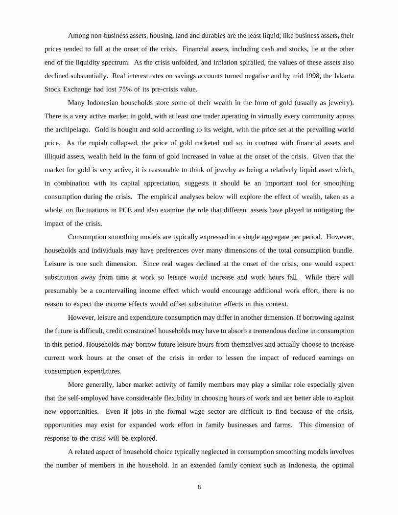
Among non-business assets, housing, land and durables are the least liquid; like business assets, their

prices tended to fall at the onset of the crisis. Financial assets, including cash and stocks, lie at the other

end of the liquidity spectrum. As the crisis unfolded, and inflation spiralled, the values of these assets also

declined substantially. Real interest rates on savings accounts turned negative and by mid 1998, the Jakarta

Stock Exchange had lost 75% of its pre-crisis value.

Many Indonesian households store some of their wealth in the form of gold (usually as jewelry).

There is a very active market in gold, with at least one trader operating in virtually every community across

the archipelago. Gold is bought and sold according to its weight, with the price set at the prevailing world

price. As the rupiah collapsed, the price of gold rocketed and so, in contrast with financial assets and

illiquid assets, wealth held in the form of gold increased in value at the onset of the crisis. Given that the

market for gold is very active, it is reasonable to think of jewelry as being a relatively liquid asset which,

in combination with its capital appreciation, suggests it should be an important tool for smoothing

consumption during the crisis. The empirical analyses below will explore the effect of wealth, taken as a

whole, on fluctuations in PCE and also examine the role that different assets have played in mitigating the

impact of the crisis.

Consumption smoothing models are typically expressed in a single aggregate per period. However,

households and individuals may have preferences over many dimensions of the total consumption bundle.

Leisure is one such dimension. Since real wages declined at the onset of the crisis, one would expect

substitution away from time at work so leisure would increase and work hours fall. While there will

presumably be a countervailing income effect which would encourage additional work effort, there is no

reason to expect the income effects would offset substitution effects in this context.

However, leisure and expenditure consumption may differ in another dimension. If borrowing against

the future is difficult, credit constrained households may have to absorb a tremendous decline in consumption

in this period. Households may borrow future leisure hours from themselves and actually choose to increase

current work hours at the onset of the crisis in order to lessen the impact of reduced earnings on

consumption expenditures.

More generally, labor market activity of family members may play a similar role especially given

that the self-employed have considerable flexibility in choosing hours of work and are better able to exploit

new opportunities. Even if jobs in the formal wage sector are difficult to find because of the crisis,

opportunities may exist for expanded work effort in family businesses and farms. This dimension of

response to the crisis will be explored.

A related aspect of household choice typically neglected in consumption smoothing models involves

the number of members in the household. In an extended family context such as Indonesia, the optimal

8

number of households per extended family presumably involves a tradeoff between taking advantages of

economies of scale in consumption and the consumption derived from individual or sub-family privacy. The

crisis may have disturbed the original equilibrium if inter-temporal smoothing across these two dimensions

are not equivalent. We hypothesize that privacy may be more substitutable over time and that households

attempt to minimize the impacts on consumption compared to privacy. If so, households should tend to

recombine and become larger during the crisis.

Indeed, one important mechanism through which non co-resident kin may spread the impact of the

crisis is through reallocation of different types of members of extended families across different households.

For example, those family members who are net consumers may relocate to relatives living in places where

consumption costs are low while those who are earners may move to help out in family businesses.

Time allocation and location choice are not the only components of the consumption bundle that

might be responsive to income shocks. Some parts of the consumption bundle (such as food) may be

poorly substitutable over time while others such as durables, semi-durable purchases and household

investments are likely to be more readily substituted over time and hence postponeable. For example,

postponement of expenditures on semi-durables such as clothing is not likely to have as large an effect on

life-time utility as postponing spending on staples. For some items, it is not obvious that there will be any

longer-run effect on utility, at least for the majority of the population; delaying preventive health care

investments is a good example. For many, such delay will be of little consequence; for some, however, the

costs may be very large.

All consumption smoothing models rely on an implicit or explicit assumption about household

expectations. We believe that the nature and magnitude of the Indonesian crisis, as described above, makes

it plausible that this crisis was largely unanticipated. A more difficult question involves household

expectations in the midst of the crisis in 1998. For example, household behavior would be quite different

if they expected the crisis to worsen considerably in the future. In that case, households may desire to save

even in 1998 to lessen the impact in the future. As further waves of IFLS are added to the database, these

dynamic issues will be addressed.

5. Results

This section summarizes our principal research findings about the ability of Indonesian households

to mitigate the impact of the crisis on their welfare during the first year of the economic crisis. The section

is organized as follows. We begin with a discussion of the measurement of household welfare and note that

household consumption and household welfare are not one in the same thing. In line with the vast majority

9

of the literature, we then lay out the basic facts in terms of per capita household consumption and discuss

the magnitude and distribution of the crisis by this metric.

The following sub-section develops measures of the community-specific "shock" that households

faced which are later used to provide insights into the mechanisms households have used to smooth welfare

during this shock. We focus on two mechanisms that appear to have played a role in the Indonesian crisis.

We first describe changes in household size and composition between the 1997 and 1998 interviews; these

reflect changes in living arrangements and migration of individual household members. Second, we present

evidence on changes in labor supply -- including sector of work and hours of work -- of household members.

This study emphasizes the role played by wealth, which is discussed in the rest of the section. We

begin with a description of wealth ownership and note that the crisis is associated with declines in the values

of some assets but increases in the values of others. We proceed to examine how the level of wealth and

its distribution among asset groups is related to reduced fluctuations in PCE. We also assess whether other

household characteristics -- particularly household structure and levels of human capital -- are associated

with greater smoothing of consumption.

5.1 Changes in household consumption

How large were the changes in household welfare that accompanied the economic crisis in Indonesia

during 1998? Which types of households experienced the largest declines? Because IFLS2 was fielded

almost entirely before prices spiraled upwards in early 1998 (Figure 1b), and IFLS2+ was fielded about a

year later, these data are uniquely well-suited to provide insights into the immediate impact of the crisis and

the extent to which households have mitigated the effects on the well-being of their members.

It is standard in this literature, to equate household per capita consumption (PCE) with the welfare

of individuals within the household. Mean levels of PCE in 1997 and 1998 are reported in the first row of

Table 1 along with the mean percentage change in PCE at the household level. The average household

reduced real consumption by almost 25% in one year.7 This is a stunning decline that is of the same

magnitude as the crisis in Russia, in the 1980s, and the first year of the Great Depression. (Throughout the

paper, all values are converted to 1997 rupiah.8)

7In this paper, consumption includes market expenditures and the imputed value of own production on foods andnon-foods. Expenditures on durables are excluded.

8Calculation of price indices is far from straightforward. See, for example, Levinson, Berry and Friedman (1999)and Thomas et al (1999) for a discussion in the context of the Indonesian crisis and Deaton and Tarozzi (2000)who examine the general issue in the Indian context. All 1993 values are inflated to 1997 prices using the priceseries for each province published by the Badan Pusat Statistik, (BPS), the Indonesian central bureau of statistics.Those prices are collected in the capital city of each provinces and the prices reported for the province capital are

10

The distribution of this decline in PCE is reported in Figure 2 which presents non-parametric

estimates of the percentage change in real household PCE between 1997 and 1998 across the distribution

of prior PCE. To avoid biases due to correlated measurement error that will arise from regressing

nPCE1998- nPCE1997 on nPCE1997, we use, on the x-axis, 1993 levels of nPCE (measured in IFLS1) to

rank households by their baseline levels of consumption.

The striking fact that emerges from the figure is the diversity of changes in PCE across households

with the initially better off household reducing their PCE by much larger percentage amounts. For example,

taking all households (in the upper left panel), the fall in consumption was 30% or more in the upper quartile

of 1993 nPCE but approximately 15% or less in the bottom quartile.

The right hand panel of Figure 2 separates households by whether they live in urban or rural areas

(in 1997). This distinction turns out to be critical in understanding the impact of the crisis. Two salient

patterns are produced by this distinction. First, percentage changes in PCE run about 10 to 15 percentage

points more negative in urban areas compared to rural places.9 Second, among households within the lower

and upper quartiles of the PCE distribution, proportionate consumption declines are largely independent of

baseline levels of PCE. In contrast, in the urban sector, we find a more uniform pattern of larger

consumption among households with higher PCE at baseline.

To be sure, for many households, the crisis in Indonesia was devastating. However, for some, it

surely brought new opportunities. For example, net food producers (particularly rice producers) benefitted

attributed to all households living in that province. (See Ravallion and Bidani, 1996.) Price deflators for 1998values are based on data collected in the IFLS community surveys which are conducted in each of the EAsincluded in the original frame. These community surveys collect information on 10 prices of standardizedcommodities from up to 3 local stores and markets in each community; in addition, prices for 39 items are askedof the Ibu PKK (leader of the local women’s group) and knowledgeable informants at up to 3 posyandus (healthposts) in each community. Using those prices, in combination with the household-level expenditure data, we havecalculated EA-specific (Laspeyres) price indices for the IFLS communities for 1997 and 1998. That price series isused to deflate all 1998 values in this paper. An alternative approach would be to use the price series for capitalcities of each province provided by BPS. Our series has two key advantages. First, in our data, there is evidencefor considerable price heterogeneity within provinces and that rural prices have increased slightly more than urbanprices during this period. Second, as shown in Figure 1, relative prices have changed substantially during this timewith food prices increasing faster than other prices. Food shares tend to be higher for poorer households and sothere is an advantage in using a deflator that is sensitive to the fact that the poorest likely faced a bigger realshock by adopting a deflator that varies across the distribution of initial PCE. We go a long way to achieving thatgoal by using an EA-specific price series -- over 50% of the variation in nPCE in IFLS is across communities.Overall, province differences in the IFLS price series mimics the BPS series although estimates of the level ofinflation are slightly higher in IFLS.

9The result that rural areas were not hit as hard by the crisis as urban areas is born out in the data fromcommunity leaders of each of the IFLS communities. In 1998 these leaders were asked how life for residents intheir community has changed in the past 12 months. About half the respondents in both sectors responded that lifewas somewhat worse. 18% of urban leaders said that life was much worse but no rural leaders said that life wasmuch worse. In fact, one quarter of rural leaders said that life was better.

11

from the increase in the relative price of food; similarly, those who produced for the export sector saw

substantial increases in the relative price of their output when the rupiah collapsed. In fact, about one-third

of households report higher levels of PCE in 1998, relative to 1997. While at least some of these apparent

increases in PCE likely reflect measurement error in expenditure (or random fluctuations in consumption),

there are at least three reasons why we think the evidence suggests that some households were better off in

1998 than in 1997.

First, a regression of change in nPCE on household and community characteristics indicates that

households in food-producing communities tended to fare better during the crisis as did households with

more members who entered the labor market between 1997 and 1998. (See Thomas et al, 1999.) Second,

in 1998, all adult respondents were asked whether their lives had improved or worsened during the previous

twelve months (using a 5-point scale). One in six reported their lives had improved whereas about 40% said

they were worse off in 1998. Third, we have aggregated these individual responses to the household level

and estimated an ordered probit relating reported change in well-being (using the same 5 point scale) to

levels of PCE, household size and location. Holding PCE in 1993 and 1997 constant, higher levels of PCE

in 1998 are associated with a significantly higher probability the household is reported as being better off

in 1998; ceteris paribus, higher PCE in 1997 is associated with lower levels of household welfare in 1998.

Thus, at the household level, changes in PCE between 1997 and 1998 are significant predictors of changes

in perceptions of household well-being, with all of these measures being collected independently of each

other. Holding constant household size in 1993 and 1997, an increase in the number of household members

in 1998 is associated with an increase in the probability a household reports itself as being better off

indicating that the addition of members to a household was viewed as welfare-improving for the average

household at the onset of the Indonesian crisis.

Returning to Table 1, we see that total household consumption declined by considerably less than

per capita consumption, particularly in rural areas. This suggests that individuals and households have

responded to the crisis by shifting living arrangements between 1997 and 1998. This is reflected in changes

in household size which, as shown in row 3, increased by 7% during this time. Changes in household size

are discussed in more detail below. For now, it is sufficient to note that studies which focus exclusively on

PCE are ignoring a potentially important smoothing mechanism.

PCE is separated into components in the next four rows. On average, per capita food consumption

was reduced by 9% whereas expenditures on non-foods took a much bigger cut and were reduced by about

a third. Part of this difference can be explained by the fact that food prices rose more rapidly than other

prices although that is probably not the full story. It is likely that households smooth welfare by re-

allocating the budget away from spending on goods that can be deferred at little immediate cost to welfare;

12

semi-durables such as clothing and household furniture are natural candidates since delay of expenditure on

these items is unlikely to affect utility as much as, say, reducing spending on basic foods. Of course, as the

period over which spending is delayed lengthens, the welfare costs of deferring expenditure rise and so the

extent to which this smoothing mechanism is adopted likely depends on expectations about future income.

(See, Browning and Crossley, 1997; Thomas et al, 2000.) In Indonesia, households substantially reduced

per capita expenditures on "deferrable" items, including clothing, furniture and spending on ceremonies,

which declined by over one-third. They also reduced investments in human capital (that is health and

education spending) by around 40%, which may have rather different implications for longer-run welfare.

The evidence in Indonesia suggests that households do smooth welfare through re-allocating the budget,

which means that the link between changes in PCE and welfare of households is not direct; this is important

to keep in mind when interpreting the evidence on household smoothing behavior below.

5.2 Measurement of economic shocks

Prior to assessing the extent to which Indonesian households were able to smooth the effects of the

economic shocks associated with the crisis, it is useful to construct a measure of the size of the shock faced

by different households which is independent of their own smoothing behavior. Using household level data

alone, it would not be possible to distinguish between a household that faced no economic disruption during

the crisis and one that was able to completely smooth the impact of the shock that they did confront.

We have explored several approaches to measuring the magnitude of the shock. The first issue to

address concerns the level of geographic aggregation. This calls for balancing at least two competing

concerns: on the one hand, the geographic unit should be small enough so that the estimated shock reflects

the nature of the local economy; on the other hand, the greater the number of estimates of the shock within

a local economy, the smaller the measurement error. If labor markets clear immediately, then all shocks

would be national as migration of labor would smooth out spatial variation in relative demand. Given its

geography (an archipelago of 13,000 islands) and its level of development and infrastructure, it seems

unlikely that the Indonesian labor market is perfect. We will present some evidence on this score below.

With this in mind, we have chosen to measure economic shocks at the level of kecamatan (which, roughly

speaking, is analogous to a county in the United States). The analyses are based on data from 85

kecamatans, 49 of which are in urban areas.10

10There are three obvious alternatives. First, we could exploit the cluster-design of IFLS and use an EA to definethe local economy. This is unsatisfactory for two reasons. First, EAs are very small (akin to a census block) andthe local economy surely casts a wider net. Second, we would exclude a substantial fraction of our householdswho had moved within the vicinity of the EA between 1993 and 1998 but were no longer living with the EA.Systematically excluding these movers from the calculation of the local economy shock will result in biased

13

The next question involves how to best characterize shocks at the local economy level. There are

several alternatives that we have explored, each with some advantages and disadvantages. A natural starting

point is the real change in the local wage. Whereas inflation in 1998 was around 80%, nominal wages in

the market sector increased by around 40%. Evidence based on IFLS demonstrates that inferences about

the impact of the crisis based on market sector wages alone misses an important part of the picture.

Specifically, there was a dramatic downward shift in real wages in the market sector of some 40% in both

the rural and urban sectors and a similar decline in real hourly earnings from self-employment in the urban

sector. However, hourly earnings of the rural self-employed declined by much less -- 15%-20% -- which

likely reflects the increased returns to food production during the crisis. (Smith et al, 2000.) Our estimates

of shocks will, therefore, be based on hourly earnings of market workers and the self-employed taken in

combination.

This raises serious issues regarding measurement since estimation of hourly earnings from self-

employment is fraught with difficulties.11 Compared with market sector earnings, self-employment income

is often very volatile; disentangling profits from returns to capital is very difficult; it is not clear how to

allocate earnings to individuals in family business with multiple members working in the activity. Moreover,

even if one can estimate earnings, the estimation of hours of work in self-employed activities is well-known

to be very hard. Given these difficulties and the fact that self-employment activities increased in importance

between 1997 and 1998 (which implies that measurement error is not likely to be differenced out), we expect

estimates of the shock based on hourly earnings to be contaminated by substantial measurement error. In

estimates of the shock if movers and stayers are not drawn from the same underlying distribution of unobservedcharacteristics. Moreover, from a practical point of view, it is very difficult to determine whether a household isliving within an EA. This issue can be side-stepped by defining the local economy in terms of the lowest level ofadministrative boundary defined in Indonesia: desa or kelurahan (village or neighborhood). (There are over60,000 desas in Indonesia.) The costs of this approach are two-fold. As with EAs, we exclude households thathave moved locally (but across a desa border). And second, several of the 90 EAs in IFLS2/2+ are located inclose proximity to one another and likely shared common shocks (10 EAs are drawn from 4 kecamatans). Thethird potential level of geographic aggregation is the kabupaten, the level above the kecamatan. Inspection of themagnitudes of estimated shocks at the kecamatan level suggested that there is heterogeneity within kabupatens andso we prefer not to aggregate to this level. A key distinction is whether a community is rural or urban. We treatthose kecamatans that contain both rural and urban areas as two separate markets. The calculation of shocks isbased only on those households that lived in the same kecamatan in 1997 and 1998. (This includes people whohad moved from their original EA between 1993 and 1997.)

11It is well-known that collection of income from self-employment in a survey setting is extremely difficult --especially, perhaps, in a low-income and substantially agricultural setting like Indonesia. Difficulties arise becauseof the need to calculate costs and net those out to compute profit, because incomes tend to be volatile over timeand often contain an important seasonality component. The panel feature of IFLS may provide some assistance.To the extent that the difficulties in measurement for a particular individual do not change between 1997 and1998, these concerns will be somewhat mitigated; inferences based on changes in self-employment incomes overthe period may not be as seriously contaminated as inferences about levels in incomes.

14

addition, our tests of smoothing revolved around changes in PCE which is measured at the household level

and it is not obvious how to aggregate individual hourly earnings so that they are comparable without

incorporating a model of family labor supply.

This suggests the first of two alternative measures: the community-specific mean change in the

logarithm of per capita income, PCY. Our second alternative is the average change in nPCE. In contrast

with hourly earnings of individuals, these measures have the advantage that they are measured at the same

level of aggregation as the outcome in the analyses -- household PCE. Relative to PCE, PCY has two

shortcomings. First, it is more likely to be measured with error and subject to contamination due to outliers.

Second, it reflects labor supply responses to the crisis.

Figure 3 displays the three measures of the community "shock". In an effort to provide insights

into the distributional impact of the crisis, we have attributed to each household the shock they faced

between 1997 and 1998 and then related those shocks to household PCE (measured in 1993).12 In the

urban sector, the "wage shock" is around -40% whereas the shock measured by PCY and PCE is close to -

20%. This gap reflects both the effect of aggregation of individual earnings to the household level and also

the existence of substantial increases in labor supply. In the rural areas, the shock is much smaller as is the

difference among the three measures of the shock. Whereas the wage shock ranges from -12% to -30%, the

shock measured by PCE and PCY lies between -12% and -20%.

Apart from an intercept difference in the urban sector, our estimates of the shocks based on PCE

and PCY are remarkably similar and yield the same inferences about the distribution of the shock.

Specifically, in both the rural and urban sectors, the shock is largest for those who were best off in 1993.

Among urban households, there is a tendency for the magnitude of the kecamatan-level shock to increase

as 1993 household PCE increases. In rural areas, the middle 50% of households faced essentially the same

shock, while those in the bottom quartile of PCE faced a slightly smaller shock.

We will use the community-mean change in nPCE as our measure of the local economy shock.

Its main disadvantage is that it may be affected by joint consumption smoothing for the community as a

whole in which case we will under-estimate the magnitude of the shock. Since our focus is on the link

between household wealth and smoothing, as long as household-specific wealth holdings and community-

specific smoothing behaviors are not related, our results should not be contaminated. Given the complexities

associated with measurement of the shock we will, in addition, take a less parametric and arguably more

robust approach and allow the community shock -- as well as all community-specific smoothing behaviors -

- be captured in a community fixed effect.

12In this figure, PCE in 1993 is used as our metric of a household's original position in the economic hierarchy tomitigate any measurement error biases induced by having 1997 nPCE on both the x and y axes.

15

5.3 Smoothing mechanisms: Household size and composition

There are many dimensions over which households may smooth' consumption in order to mitigate

the welfare reducing consequences of a severe economic shock. One often ignored dimension involves

changes in household size and composition. In order to share fixed living expenses such as housing and food

preparation, households may try to combine into larger units, forgoing at least temporarily the luxury of

some privacy. Similarly, those households hit more severely may send some members to live with other

households less severely affected by the crisis or to places where the cost of consumption may be lower.

Consumption costs may not be the only reason for reshuffling of household members. Spatial variation in

the size of economic disruptions may lead some household members to relocate to places where the

prospects for generating income are better.

The upper panel of Figure 4 plots the change in household size between 1997 and 1998 in the urban

and rural sectors.13 The figures indicate that, on average, IFLS households became somewhat larger during

the economic crisis, an increase that was greater for households with higher levels of 1993 per capita

consumption. More revealing, however, is the separation of these household size trends by rural and urban

residence. In the urban sector, the bottom quarter of households as ranked by their 1993 PCE actually lost

household members during the crisis while urban households above median 1993 PCE gained new members.

In contrast, across the entire distribution of 1993 PCE, household size was expanding in the rural sector. This

expansion was small for the poorest rural households, but reached about half an additional member for the

most well-off rural households.

To see why the direction of household size changes may have differed between the urban and rural

sector, we have examined changes in relative hourly earnings (or wages for shorthand) in the two sectors.

We have arrayed the 1997 distribution of wages by percentiles and found the corresponding percentiles in

the urban and rural wage distribution that matched each aggregate percentile wage. Given that the

distribution of urban wages lies above that of rural wages, these matched urban wages were at a lower

percentile and the matched rural wages at a higher percentile than the aggregate percentile wage. For each

sector of residence, we then computed the percent change in the wage between 1997 and 1998 yielding a

difference in rural wages and a difference in urban wages at the same real wage.

Figure 5 presents our (smoothed) estimates of the urban-rural differential in the wage decline during

the year of the shock separately for male wage earners across the 1997 wage distribution. The patterns are

remarkably systematic. Among the least skilled men, there was about a 15% decrease in urban wages

13It is possible that the estimates in the figure slightly overstate the increase in household size since largerhouseholds were somewhat easier to find and therefore less likely to attrit in IFLS2+. Given the very low attritionrate (<1.5% of households), we do not think this is a serious concern.

16

relative to the drop in rural wages. This greater relative wage deterioration in urban markets monotonically

declines as we move up the wage (skill) distribution until there is a roughly equal reduction of male urban

and rural wages at the highest wage (skill) levels.

These between sector relative wage changes map neatly into the household size changes documented

in the upper panel of Figure 4. The Indonesian economic crisis hit unskilled labor markets harder in urban

areas than in rural settings. Some low skill workers in poor urban households exited the urban sector to

find work in the rural sector. While doing so, many of them apparently joined middle income or higher

income households in rural areas

Additional insight can be obtained on how changes in household membership are operating by

examining the characteristics of those who enter or leave the household. To do so, we separated household

members by gender and into four age groups-0-14, 14-25, 25-54, and 55+. These changes in household size

and composition are subdivided by quartiles of PCE in Table 2.

Relative to changes in the urban sector, increases in household size are larger in the rural sector

particularly in the bottom and top quartiles of PCE. The rural-urban differential is sharpest among older

rural women. In the bottom quartile of 1993 PCE urban households, the most striking pattern is that male

and female children under age 14 apparently left their original household. These young children may have

been accompanied by their mothers since there was also a decrease in women ages 25-54. No similar trends

exist among rural households in the bottom quartile of PCE. In the top quartile of PCE in both the rural

and urban sectors, there was a large increase in the number of men in the prime age worker category (ages

15-54) and a slightly smaller increase in the number of women in this age range.

The evidence indicates that dependents tended to have exited urban households that were poorest

(measured by PCE in 1993) and moved to lower-cost rural areas. At the same time, households that were

better off in 1993 have been net recipients of working age adults which likely reflects the fact that these

households were better able to exploit new opportunities to generate income as the crisis unfolded, possibly

because the households had land or other forms of capital.

5.4 Smoothing mechanisms: Labor supply and number of workers

In addition to the exit or entry of additional people into the household, a household may attempt to

adjust to the crisis by altering the labor supply decisions of its members. On the demand side, some workers

especially in the formal wage sector may have lost their jobs and are no longer working. Other family

members may have increased their work effort by helping out in family businesses.

There are several aspects of total family labor supply that we examine in this paper -- the number

of workers in the family and the hours of work. Table 3 lists changes between 1997 and 1998 in the number

17

of workers in each household in the rural and urban sector. While there was a greater increase in household

membership among rural households, there was actually a greater increase in number of workers in urban

areas. This indicates that the increase in number of workers in urban households was not simply at the

extensive margin -- i.e. adding new members -- but also resulted from additional work by members already

there. The increase in numbers of workers was concentrated in the wage sector in urban areas and in the

family business in rural areas.

The last three rows of Table 3 focus on hours of work. The total number of hours worked by all

household members increased substantially in both the rural and urban areas: the average household spent

an additional 25 hours at work per week after the onset of the crisis. The per worker increase in hours

worked was about 10 hours per week. It turns out that these additional hours represent the combination of

a reduction in the extent of part time work and, for some full-time workers, a large increase in hours spent

working, particularly among the self-employed.

Table 3 indicates that one important adjustment mechanism to the economic crisis was a sharp

increase in hours worked. The lower panel of Figure 5 presents more detail about the nature of that

adjustment by relating the percent change in total household hours worked by each household with 1993

nPCE. There was a very large increase of over twenty percent in total household hours worked in the rural

sector. These increases were roughly independent of 1993 PCE in urban areas, but were roughly U shaped

in rural areas. The large increase in work effort in response to the crisis is one reason why changes in

nPCY are higher than per cent changes in wages in Figure 3.

The data presented in this section highlights two important adjustments households made in the face

of this crisis. First, households consolidated and became larger, presumably to economize on fixed

consumption costs. The composition of households also changed, especially in urban areas, so that members

who were primarily consumers (such as young children and their mothers) left while earners moved in. The

second adjustment was a significant increase in total work effort by the household.

5.5 Smoothing mechanisms: Wealth

For those households that own assets prior to an economic shock, their wealth may serve as a buffer

to soften the potential blow to their consumption. As central as the total value of assets is likely to be,

portfolio composition may also be important since the more liquid an asset, the more readily it may be

converted to resources to finance consumption. Many economic and financial crises, including the

Indonesian case, have been accompanied by substantial swings in the relative prices of assets. The

associated capital gains and losses are also likely to result in consumption and savings adjustments by

households. We explore each of these mechanisms below.

18

Distribution of ownership of wealth

IFLS pays considerable attention to the collection of information on wealth. The rates of ownership

in 1997 and 1998 are reported in Table 4. Values of wealth in 1997 and 1998 are reported in Table 5 in

thousands of 1997 Rp. Because the distribution is extremely right skewed, the value at the median, bottom

and top quartile and bottom and top decile are reported in the table.

Essentially all Indonesian households owned some wealth in both 1997 and 1998. The total value

of business and non-business wealth of the median urban household is about Rp 10 million and the median

rural household owns about Rp 6 million in such assets. (This is equivalent to about a year and a half of

consumption for the median household.) In both sectors, the median for total assets has remained

remarkably stable through the crisis. In fact, in the rural sector, the distribution of wealth has remained

reasonably constant below the median but has stretched out substantially above the median. The reverse is

true in urban areas, where the right hand tail of the wealth distribution has been substantially curtailed and

the left tail has expanded.

These differences are primarily a reflection of the fact that business wealth has tended to increase

(or at least fall less than non-business wealth) between 1997 and 1998. In the rural sector, four out of five

households own wealth that is associated with a business (typically farming) whereas two out of three urban

households own a business that involves some assets. As noted above, self-employment activities --

particularly those revolving around the production of food -- became relatively more attractive as the price

of rice and other crops spiraled up. Households apparently responded by building up their family businesses.

Excluding business wealth, household wealth has declined throughout the distribution among rural

households and it has declined for all households above the median in the urban sector.

Excluding business wealth, the dominant assets owned by households are their home and land. Over

ninety percent of rural and seventy percent of urban households own their own home with almost no change

in ownership during the crisis. The value of houses declined between 1997 and 1998. Commercial property

values, particularly in the largest urban centers, plummeted as construction contracts were canceled and

many developers went out of business. The collapse of the banking system -- and lack of credit -- took its

toll on the home property market. Arable land, on the other hand, likely became more valuable although

the absence of credit likely muted activity in this market.

Turning to more liquid assets, about one-quarter of rural households and 40% of urban households

keep some of their wealth in the form of cash, bonds or stocks. A higher fraction of households store wealth

in the form of gold (as jewelry), particularly in rural areas. This likely reflects the fact that financial services

are much less accessible in rural areas, relative to urban areas, whereas there is an active market in gold

throughout Indonesia. Moreover, whereas aggregate ownership rates for all other assets have remained

19

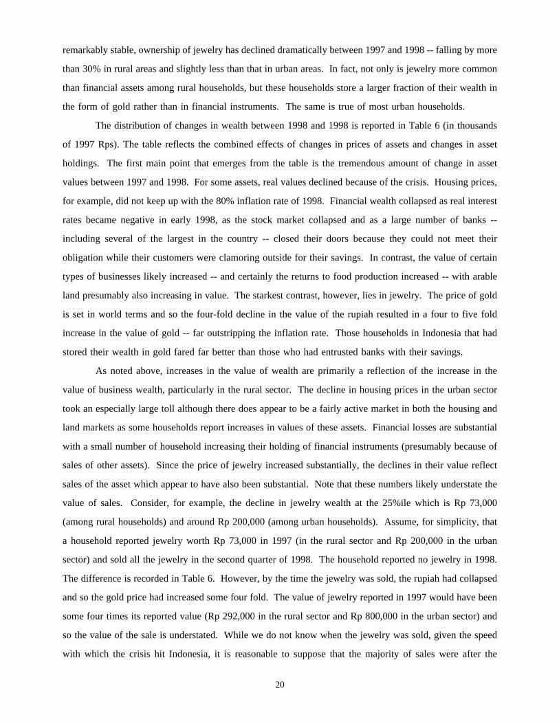
remarkably stable, ownership of jewelry has declined dramatically between 1997 and 1998 -- falling by more

than 30% in rural areas and slightly less than that in urban areas. In fact, not only is jewelry more common

than financial assets among rural households, but these households store a larger fraction of their wealth in

the form of gold rather than in financial instruments. The same is true of most urban households.

The distribution of changes in wealth between 1998 and 1998 is reported in Table 6 (in thousands

of 1997 Rps). The table reflects the combined effects of changes in prices of assets and changes in asset

holdings. The first main point that emerges from the table is the tremendous amount of change in asset

values between 1997 and 1998. For some assets, real values declined because of the crisis. Housing prices,

for example, did not keep up with the 80% inflation rate of 1998. Financial wealth collapsed as real interest

rates became negative in early 1998, as the stock market collapsed and as a large number of banks --

including several of the largest in the country -- closed their doors because they could not meet their

obligation while their customers were clamoring outside for their savings. In contrast, the value of certain

types of businesses likely increased -- and certainly the returns to food production increased -- with arable

land presumably also increasing in value. The starkest contrast, however, lies in jewelry. The price of gold

is set in world terms and so the four-fold decline in the value of the rupiah resulted in a four to five fold

increase in the value of gold -- far outstripping the inflation rate. Those households in Indonesia that had

stored their wealth in gold fared far better than those who had entrusted banks with their savings.

As noted above, increases in the value of wealth are primarily a reflection of the increase in the

value of business wealth, particularly in the rural sector. The decline in housing prices in the urban sector

took an especially large toll although there does appear to be a fairly active market in both the housing and

land markets as some households report increases in values of these assets. Financial losses are substantial

with a small number of household increasing their holding of financial instruments (presumably because of

sales of other assets). Since the price of jewelry increased substantially, the declines in their value reflect

sales of the asset which appear to have also been substantial. Note that these numbers likely understate the

value of sales. Consider, for example, the decline in jewelry wealth at the 25%ile which is Rp 73,000

(among rural households) and around Rp 200,000 (among urban households). Assume, for simplicity, that

a household reported jewelry worth Rp 73,000 in 1997 (in the rural sector and Rp 200,000 in the urban

sector) and sold all the jewelry in the second quarter of 1998. The household reported no jewelry in 1998.

The difference is recorded in Table 6. However, by the time the jewelry was sold, the rupiah had collapsed

and so the gold price had increased some four fold. The value of jewelry reported in 1997 would have been

some four times its reported value (Rp 292,000 in the rural sector and Rp 800,000 in the urban sector) and

so the value of the sale is understated. While we do not know when the jewelry was sold, given the speed

with which the crisis hit Indonesia, it is reasonable to suppose that the majority of sales were after the

20

collapse of the rupiah in early 1998. (To put the change in the value of jewelry into some perspective, it

is equivalent to about 4 months of food consumption in the average rural household and 9 months in the

average urban household.)

Asset markets

The evidence above presents a picture of wealth ownership that is far more equitable in Indonesia

than in any developed country. Home ownership is very high, businesses are common and the majority of

households own some form of liquid wealth. Since the banking system all but collapsed in Indonesia in

early 1998, if this wealth is going to serve to smooth consumption, there must also be an active market for

the assets. We do not know details about sales and purchases of assets in IFLS. However, Table 7 presents

evidence that speaks to this issue. For each asset group, the table records the percentage of households that

owned the asset in both years, that sold all their assets, new owners and the percentage that did not own in

either year. These percentages are recorded for households in each quartile of the PCE distribution

(measured in 1997).

There is some evidence that business assets were sold, particularly in the urban sector, and that a

substantial fraction of households started new businesses between 1997 and 1998. Of households that did

not own any business assets in 1997, about 60% of rural and 40% of urban households had acquired some

business assets by 1998. There also appears to be a very active land market with the poorest households

most likely to enter that market, presumably by buying low price tracts of land. It is likely that most of

these acquisitions were intended for the production of food although it is worth noting that households were

not entering both the land and business asset market at the same time. For example, of those who entered

the land market, only 15% also entered the business asset market. A similar fraction of the new business

asset owners were new land owners. Relative to these markets, the housing market is comparatively thin.

Whereas households at the top of the PCE distribution are more likely to own financial assets,

jewelry ownership is only modestly linked to PCE although (median) values are positively associated with

PCE in both cases. A very large fraction of households that owned financial assets in 1997 had exited the

market by 1998 and a roughly equal fraction entered the market. (There was a slight increase in ownership

of financial assets in the rural sector and net decline in the urban sector.)

There is clear evidence of an active jewelry market with a substantial fraction of households selling

their gold, possibly to finance consumption. Specifically, over half the households in the rural sector and

close to one-third of urban households who owned jewelry in 1997 had sold all their holdings by 1998.

There are considerably fewer households who entered the jewelry market during this time, which should not

be surprising given it had become relatively expensive. The fraction of households who sold their holdings

21

is approximately constant across the distribution of PCE as is the fraction of new entrants indicating that

gold transactions involved households at all levels of consumption.

It is not only the IFLS household data that clearly points to an active jewelry market in both rural

and urban Indonesia and a more limited role of financial services in rural Indonesia. The importance of gold

as a savings method is confirmed in the anthropological literature on family economics. The acquisition of

gold, usually in the form of jewelry, is seen as an investment and has long been an important way to save

money in Indonesia. Women, in particular, buy gold earrings, rings, and bracelets with savings from their

household budget, their wages, or from arisan winnings (Papanek and Schwede, 1988; Gondowarsito, 1990;

Wolf, 1991; Adioetomo et al., 1997). Such gold jewelry, typically 18 or 22 carat, is priced by weight, and

can be quickly resold for cash in times when the household needs money (Wolf, 1991). Stores that buy and

sell gold are common, as are more informal traders and brokers, many of whom are women (Papanek and

Schwede, 1988; Sullivan, 1994).

Further confirmation is provided in the IFLS community surveys which asked community leaders

to identify the ways that community residents save money. Gold was mentioned as a form of savings in

both rural and urban areas, while financial instruments such as CDs and stocks were much more commonly

identified by urban informants. In rural areas, opportunities to buy and sell gold are more available than

opportunities to save money through formal credit institutions. The IFLS community survey queried

community leaders in each IFLS community about whether they could identify a private bank or any of six

government credit institutions. Those who could were asked to estimate the distance to the credit institution

from the community center. The median distance to a government credit institution was 6 kilometers in rural

areas, but only 1 kilometer in urban areas. The difference is much more stark for private banks. While 75%

of urban informants could identify a private bank used by community members, only 40% of rural

informants could do so. In those communities where a bank could be identified, the banks were an average

of 2.5 kilometers from urban communities, but 13.4 kilometers from rural communities.

5.6 Regression models of characteristics associated with smoothing PCE

In this section, we summarize regression results which seek to identify the characteristics of

Indonesian households associated with greater smoothing of per capita consumption. The dependent variable

in each case is the change in nPCE between 1997 and 1998, ∆ nPCE, measured at the household level in

IFLS2 and IFLS2+ and converted to 1997 Rupiah. The economic shock in the local (kecamatan) economy

22

is measured by ∆ nPCE averaged over all households who lived in the kecamatan in both 1997 and 1998.14

Tests of smoothing behavior are based on the interaction between our measure of the local economy shock

and household characteristics that are likely to be associated with reducing fluctuations in nPCE. In each

case, if the characteristic is associated with greater smoothing of PCE, the interaction will be negative.

Regressions are reported separately for rural and urban households. Two models are presented for

each regression. The first includes all households. The second excludes those households that have changed

household size in order to check that our results are not driven by changes in household size and

composition. Similarity of results in each pair will indicate that the array of demographic controls included

in each regression does a good job of capturing the differences in smoothing behaviors across these groups

of households. The regressions include an extensive set of controls to capture differences in household and

community characteristics. In all models that include interactions with the local economy shock, we present

estimates with and without kecamatan fixed effects. The fixed effects estimates sweep out the main effects

of spatial variation in the magnitude of the shock as well as all other changes in the local economy including

changes in prices. The table reports only the coefficients of main interest.

As a starting point, the specifications in Panel A provide an estimate of the magnitude of the effect

of the community shock on household PCE. In both the rural and urban sector, we cannot reject the

hypothesis that this effect is unity. This may be interpreted as indicating that our measure of the local

economy shock has the same impact on all households; it is also consistent with the measure reflecting the

local shock after all community-level smoothing has taken place.

The rest of Table 8 focusses on the extent to which household-specific smoothing is associated with

three sets of characteristics: household wealth, household size and the level of human capital, all of which

are measured in 1997. In general, since wealth and human capital are positively correlated, the inclusion

of both characteristics in the regressions provides an opportunity to isolate a wealth effect from an

information or background effect.

We begin with levels of human capital, measured by the education of the household head. A better

educated person may be more able to exploit new opportunities that arise in times of upheaval -- as in

Indonesia in the late 1990s -- and the better educated may be better able to make ends meet in bad times.

In both the rural and urban sector, the better educated do appear to be more able to smooth

fluctuations in PCE. Relative to households whose head has no education, those with heads who have more

14Households that moved out of a kecamatan between 1997 and 1998 are assumed to have faced the shock in their1997 location. Households that did not live in a kecamatan that included an IFLS EA were assigned the averageshock for their province and sector of residence in 1997. The regressions include a control for these households,for whom the shock may be measured with greater error. Estimates of the local economy shock faced by aparticular households do not include that household in the calculation.

23

than primary schooling (in the urban sector) and those with any education (in the rural sector) have

significantly smaller fluctuations in nPCE for any given local economy shock. When kecamatan effects

are included in the model, the coefficient estimates are smaller but the standard errors are considerably larger

and so, in general, the effects are no longer statistically significant. A significant amount of variation in

education is across kecamatans limiting our statistical ability to draw strong conclusions about schooling

effects when the models include local economy fixed effects. There is also a suggestion that part of the

additional smoothing observed for higher human capital households takes place through changes in

household size. When we restrict attention to households with no change in size, the effect of the household

head’s education is greater.

The second set of smoothing mechanisms we investigate highlights the role of household size. We

noted above that there have been significant changes in household size and composition between 1997 and

1998 and those changes may serve as a cushion to smooth consumption. Empirical support for that

hypothesis is limited to the urban sector, where the interaction between household size and the local

economy shock is negative and significant.

We have also explored whether there are important household composition effects. The analyses

yielded one consistent pattern: urban households with more older women appear to be especially able to

smooth PCE. This effect is considerably muted in magnitude among those households that do not change

household size (for they would need to swap an older woman for someone else). There are no significant

benefits associated with having more household members in rural areas.15

We turn next to the effects of wealth (as of 1997). We interpret the direct effects of wealth (in

column 2) as indicative of the distributional impact of the crisis, controlling household and community

characteristics. There are no direct wealth effects in urban areas, but negative direct effects in rural places.

This indicates that, within rural communities, households with more wealth in 1997 experienced larger

changes in their consumption levels.

Our results on the link between consumption smoothing and wealth are based on the interaction

between wealth and the local economy shock (reported in column 3). There are likely to be two competing

effects. On the one hand, assets may be depleted and those resources used to smooth consumption; on the

other hand, there may be capital gains (or losses) which will also affect savings and consumption choices.

In general, wealth appears to play no role at all in smoothing nPCE in urban households. This is true in

15While we have attempted to explore the link between consumption smoothing and employment status (in 1997)of household members, we have failed to identify a simple pattern. We suspect that we will need to develop morecomplex structures that take into account both changes in household composition and the probability a particulartype of household member will enter the labor force between 1997 and 1998. Those analyses are left for futurework.

24

aggregate and also when we distinguish components of wealth. In the rural sector, there is a suggestion that

as the magnitude of the local economy shock increased, households with more wealth in 1997 were better

able to smooth their consumption.

Recall from the discussion above that the impact of the crisis on wealth differed dramatically across

assets groups. For some, such as jewelry, the depletion and capital gains effects are reinforcing and we

would expect those assets to play a role in smoothing consumption (in which case the interaction between

wealth and the local economy shock should be negative). For other assets, such as financial assets and

housing, the capital gains and depletion effect operate in different directions yielding no predictions on their

role in smoothing consumption. With this in mind, we have re-estimated the models in Table 8 with the

same set of covariates and interactions but explicitly distinguish the major asset classes. The results are

reported in Table 9.

Mirroring our result on total household wealth, there is no evidence that any components of wealth

have a significant impact on consumption smoothing among urban households. Results for those households

are not reported. The results for education and household size are unaffected by the separation of wealth

into components and so those results are not repeated. Table 9 reports, for rural households, the direct

effects of components of wealth along with their interactions with the local economy shock. We have

separated business wealth; housing, other wealth and financial wealth; land; and jewelry.

There is no evidence that rural households with more business wealth in 1997 were better able to

smooth fluctuations in PCE at the onset of the crisis. The same inference emerges for those with greater

wealth in housing, financial assets or other wealth. Two dimensions of wealth do appear to be associated

with smoothing consumption: land and jewelry.

Among households that did not change household size, more land is associated with greater

smoothing and it is significant at 10%. Roughly two-thirds of Indonesian households are land owners and

there is an active market for land. The link between land ownership and consumption smoothing is not

likely to be a reflection of greater income from a family business in agriculture, since we have distinguished

business wealth in the regressions and we see no evidence that business wealth (most of which is land and

agricultural equipment) is associated with greater smoothing. The fact that land is used to smooth

consumption among those households that do not change in size suggests there are complex interactions

between changes in wealth and changes in family structure.

The clearest evidence that wealth is associated with consumption smoothing emerges for jewelry.

The interaction term is much larger in magnitude than that of land and it is significant at a 5% size of test

in three of the models. The magnitude of the estimated effect is slightly larger in models that include

25

kecamatan fixed effects (but the standard errors increase and the effect is not significant among households

that did not change size. We suspect this primarily reflects lack of power.)

That gold should serve as a mechanism for smoothing consumption is not surprising. First, we have

noted that its value more than quadrupled at the onset of the crisis. Second, we noted above that gold is

owned by households throughout the income distribution. Third, there is an active market in gold across

the Indonesian archipelago. Fourth, there is evidence in IFLS that many households sold gold during the

hiatus between the two survey rounds.

A tantalizing fact revolves around the distribution of jewelry within households. The IFLS wealth

module asks about the share of each asset group owned by the respondent and the share owned by the

respondent’s spouse. In IFLS2, among those households that own jewelry, 20% report that it is owned

jointly with the spouse. In 75% of the households, the woman owns all the jewelry and males own the

jewelry in only 5% of households. Moreover, 85% of the value of jewelry is attributed to women and only

15% to men -- facts that are consistent with the anthropological evidence discussed above. In the context

of a collective model of household decision-making, the (exogenous) increase in the price of gold associated

with the crisis increased the value of assets owned by a woman and improved her "bargaining" position

relative to her husband. Evidence in IFLS2/2+ suggests that jewelry sold between 1997 and 1998 was more

often under the control of women since the fraction of households in which men and women jointly own

jewelry increased by 25% (from 20% to 25%). This suggests that preferences for consumption smoothing

may not be the same among all household members and, therefore, that within household dynamics in

decision-making may be extremely complex. These issues will be explored in detail in future work.

6. Conclusions

1998 marked a dramatic and unexpected reversal of economic fortunes in Indonesia. After 30 years

of sustained growth, the economy shrank by about 15% in one year. Using data that were specially collected

to measure the immediate effects of the economic and financial crisis, we have shown that there is

considerable diversity in the magnitude of the economic shock, as measured by changes in household PCE.

For some, the crisis has been devastating; for others it has brought new opportunities.

Rural and urban households in Indonesia have adopted a wide array of mechanisms to mitigate the

deleterious impact of the shock -- and to exploit the new opportunities that have emerged since the onset

of the crisis. Households and families have re-organized living arrangements with dependents tending to

move to lower-cost locations and working age family members joining households that are able to absorb

additional workers. There is also evidence that in spite of the collapse of hourly earnings, labor supply has

increased. On net, individuals have entered the labor force and many of those who were working prior to

26

the crisis have increased their hours of work. Changes in the allocations of time of household members has

been accompanied by re-arrangement of other dimensions of the budget. There is evidence that households

have cut back spending on "deferable" items (such as clothing, household furniture and similar semi-

durables) while maintaining real expenditures on foods.

The role of wealth in strategies adopted to smooth consumption has played a central role in this

paper. In contrast with developed countries, the vast majority of Indonesian households store some wealth

in the form of assets. As the rupiah collapsed and inflation spiralled, the value of most assets declined very

substantially in value. This capital loss should dampen the impact of wealth on consumption smoothing.

Gold stands out as being different. Since the price of gold is set in world terms, its value increased four-fold

in early 1998, when the rupiah collapsed. Moreover, a good deal of evidence indicates there is a very active

market in gold throughout the Indonesian archipelago. We see clear evidence that rural households used

gold to smooth their consumption. There is more limited evidence that rural households with more land

were better able to smooth their consumption.

The picture that emerges from the empirical evidence in the IFLS is one of tremendous diversity and

great complexity in the response of households to the massive economic and financial crisis in Indonesia.

Households appear to use all means at their disposal to smooth out the impact of the crisis on their current

and future welfare.

27

References

Adioetomo, Toersilaningsih, Asmanedi, Hendratno, Fitriwati, Egglestone, Hardee, and Hull. 1997. "Helpinghusband, maintaining harmony." Demographic Institute. University of Indonesia.

Alamgir, M. (1980). Famine in South Asia: Political economy of mass starvation, Cambridge, MA:Oelgeschlager, Gunn and Hain Publishers.

Browning, M. and T. Crossley. (1997) "Consumption smoothing and the replacement of durables during anunemployment spell", mimeo.

Cameron, L. (1999). "Indonesia: a quarterly review," Bulletin of Indonesian Economics Studies 35(1), April.

Cox, D., and E. Jimmenez. (1998). "Risk sharing and private transfers: What about urban households?"Economic Development and Cultural Change, 46.3:621-637.

Deaton, A. (1992) Understanding consumption, Oxford:Clarendon Press.

Deaton, A. and A. Tarozzi. (2000) "Prices and poverty", mimeo.

Gondowarsito, R. (1990) "Transmigrasi Bedol Desa: inter-island village resettlement from Wonogiri toBengkulu." Bulletin of Indonesian Economic Studies. 26(1):48-68.

IMF. (1999). "World Economic Outlook: International financial contagion," World Economic and FinancialSurveys, IMF, Washington, DC.

Fafchamps, M., C. Udry and K. Czukas. (1998). "Drought and saving in West Africa: are livestock a bufferstock?," Journal of Development Economics, 55.2:273-305.

Frankenberg, E., D. Thomas and K. Beegle. (1999) "The Real Costs of Indonesia’s Economic Crisis:Preliminary Findings from the Indonesia Family Life Surveys." DRU-2064-NIA/NICHD (1999).Santa Monica, CA: RAND.

Levinsohn, J., S. Berry, and J. Friedman. (1999) "Impacts of the Indonesian economic crisis: Price changesand the Poor," NBER Working Paper 7194.

Murruggarra, E. (1996). "Economic shocks, agricultural production and family composition", mimeo, UCLA.

Papanek, H. and L. Schwede. (1988) "Women are good with money: earning and managing in anIndonesian city." Pp. 71-98 in Dwyer and J. Bruce (eds) A Home Divided: Women and Income in theThird World. Stanford, CA: Stanford University Press.

Platteau, J.-P. (1991) "Traditional systems of social security and hunger insurance: Some lessons from theevidence pertaining to Third World countries", in E. Ahmad et al., (eds.) Social security indeveloping countries, Oxford: Clarendon Press.

Rosenzweig, M. R. (1988). "Risk, implicit contracts and the family in rural areas of low-income countries,"Economic Journal, 98.393:1148-70.

Rosenzweig, M. R. (1996). "Labor markets in low income countries" in H. Chenery and T. N. Srinivasan,(eds.) Handbook of Development Economics, North Holland.

Rosenzweig, M. R. and O. Stark. (1989). "Consumption smoothing, migration, and marriage: Evidence fromrural India", Journal of Political Economy, 97.4:905-26.

28

Rosenzweig, M. R. and K. Wolpin. (1993). "Credit market constraints, consumption smoothing and theaccumulation of durable production assets in low income countries: Investments in bullocks inIndia", Journal of Political Economy, 101.2:223-44.

Smith, J. P., D. Thomas, K. Beegle, E. Frankenberg and G. Teruel. (2000) "Wages, employment andeconomic shocks: Evidence from Indonesia", forthcoming in Journal of Population Economics

Sullivan, N. 1994. Masters and managers: a study of gender relations in urban Java. St. Leonards,Australia: Allen and Ulwin.

Thomas, D., E. Frankenberg, K. Beegle and G. Teruel. (2000). "Household budgets, household compositionand the crisis in Indonesia: Evidence from longitudinal household survey data", mimeo.

Thomas, D., E. Frankenberg and J. P. Smith. (2000) "Lost but not forgotten: Attrition and follow-up in theIndonesia Family Life Survey", mimeo.

Townsend, R. (1994) "Risk and insurance in village India", Econometrica, 62:539-91.

Udry, C. (1994). "Risk and insurance in a rural credit market - an empirical investigation", Review ofEconomic Studies, 61.3:495-526

Wolf, D. (1991) "Female autonomy, the family, and industrialization in Java." Pp. 128-148 in R. Blumberg(ed). Gender, Family, and Economy: The Triple Overlap. London:Sage Publications.

29

TABLE 1: Household consumption1997, 1998 and changes for all HHsMeans and (standard errors)

1997 Rp000s 1997 1998 %change

Per capita household consumption 176 117 -23[12] [9] [2]

Total household consumption 629 491 -16[48] [42] [1]

Household size 4.33 4.53 7[0.05] [0.04] [0.8]

Composition of per capita household consumptionFood 79.7 68.9 -9

[4.9] [7.4] [2]

Non foods 95.2 48.4 -34[10.2] [2.2] [2]

Deferable items 9.1 6.4 -35(Clothing, furniture and ceremonies) [0.4] [0.4] [3]

Human capital investments 9.0 5.7 -37(Health and education) [0.6] [0.3] [3]

Note: Consumption measured in thousands of 1997 Rupiah. % change is nPCE1998-nPCE1997. 1,971 households interviewed in 1997 and 1998 included in sample.

TA

BL

E2:

:H

ouse

hold

size

and

com

posi

tion

byqu

arti

leof

HH

PC

ESi

zean

dco

mpo

sitio

nin

1997

,19

98an

dch

ange

betw

een

thos

eye

ars;

HH

PCE

mea

sure

din

1993

%ile

of19

93PC

E:

0-25

%ile

26-5

0%ile

51-7

5%ile

76-1

00%

ileC

hara

cter

istic

1997

1998

Cha

nge

1997

1998

Cha

nge

1997

1998

Cha

nge

1997

1998

Cha

nge

Rur

al%

noch

ange

inH

Hsi

ze58

.058

.158

.454

.5

HH

size

4.74

4.79

0.05

4.22

4.40

0.18

4.13

4.36

0.23

3.34

3.80

0.46

#m

ales

age

0-14

1.01

1.00

-0.0

10.

820.

80-0

.02

0.71

0.70

-0.0

10.

500.

580.

0815

-24

0.38

0.37

-0.0

10.

330.

410.

080.

380.

450.

070.

230.

320.

0825

-54

0.71

0.72

0.01

0.67

0.68

0.01

0.64

0.69

0.05

0.56

0.65

0.08

>=

550.

290.

290.

000.

260.

290.

030.

290.

320.

030.

230.

250.

01#

fem

ales

age

0-14

0.87

0.89

0.02

0.75

0.75

0.00

0.70

0.70

0.00

0.56

0.63

0.06

15-2

40.

370.

380.

000.

320.

340.

020.

360.

420.

050.

320.

360.

0525

-54

0.81

0.80

-0.0

10.

780.

78-0

.01

0.79

0.79

0.00

0.66

0.72

0.06

>=

550.

290.

330.

040.

290.

360.

070.

260.

300.

030.

270.

310.

04

Urb

an%

noch

ange

inH

Hsi

ze55

.857

.857

.851

.3

HH

size

5.03

4.92

-0.1

14.

845.

010.

174.

534.

760.

224.

034.

370.

35#

mal

esag

e0-

140.

770.

75-0

.02

0.79

0.80

0.01

0.72

0.76

0.04

0.50

0.53

0.03

15-2

40.

480.

44-0

.04

0.52

0.57

0.05

0.51

0.57

0.06

0.48

0.54

0.06

25-5

40.

790.

77-0

.02

0.77

0.85

0.08

0.90

0.93

0.03

0.82

0.91

0.09

>=

550.

260.

300.

040.

200.

190.

000.

190.

18-0

.01

0.22

0.26

0.05

#fe

mal

esag

e0-

140.

860.

79-0

.08

0.83

0.79

-0.0

40.

590.

600.

010.

480.

500.

0215

-24

0.55

0.58

0.03

0.48

0.53

0.05

0.42

0.44

0.02

0.43

0.47

0.04

25-5

40.

970.

92-0

.05

0.89

0.92

0.03

0.93

1.00

0.07

0.83

0.89

0.07

>=

550.

350.

380.

030.

350.

360.

000.

270.

260.

000.

280.

290.

01

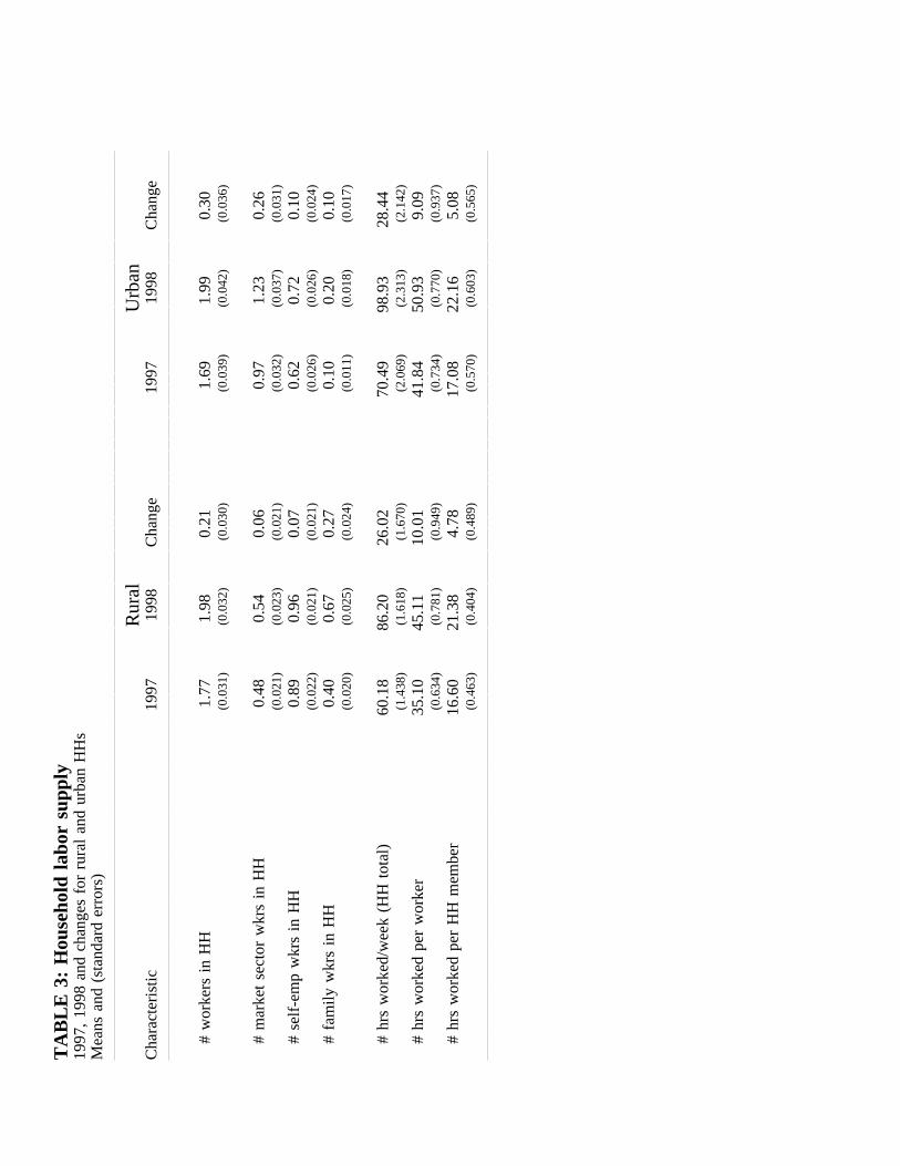
TA

BL

E3:

Hou

seho

ldla

bor

supp

ly19

97,

1998

and

chan

ges

for

rura

lan

dur

ban

HH

sM

eans

and

(sta

ndar

der

rors

)

Rur

alU

rban

Cha

ract

eris

tic19

9719

98C

hang

e19

9719

98C

hang

e

#w

orke

rsin

HH

1.77

1.98

0.21

1.69

1.99

0.30

(0.0

31)

(0.0

32)

(0.0

30)

(0.0

39)

(0.0

42)

(0.0

36)

#m

arke

tse

ctor

wkr

sin

HH

0.48

0.54

0.06

0.97

1.23

0.26

(0.0

21)

(0.0

23)

(0.0

21)

(0.0

32)

(0.0

37)

(0.0

31)

#se

lf-e

mp

wkr

sin

HH

0.89

0.96

0.07

0.62

0.72

0.10

(0.0

22)

(0.0

21)

(0.0

21)

(0.0

26)

(0.0

26)

(0.0

24)

#fa

mily

wkr

sin

HH

0.40

0.67

0.27

0.10

0.20

0.10

(0.0

20)

(0.0

25)

(0.0

24)

(0.0

11)

(0.0

18)

(0.0

17)

#hr

sw

orke

d/w

eek

(HH

tota

l)60

.18

86.2

026

.02

70.4

998

.93

28.4

4(1

.438

)(1

.618

)(1

.670

)(2

.069

)(2

.313

)(2

.142

)

#hr

sw

orke

dpe

rw

orke

r35

.10

45.1

110

.01

41.8

450

.93

9.09

(0.6

34)

(0.7

81)

(0.9

49)

(0.7

34)

(0.7

70)

(0.9

37)

#hr

sw

orke

dpe

rH

Hm

embe

r16

.60

21.3

84.

7817

.08

22.1

65.

08(0

.463

)(0

.404

)(0

.489

)(0

.570

)(0

.603

)(0

.565

)

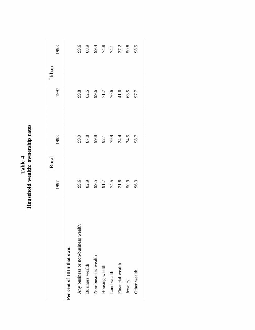
Tab

le4

Hou

seho

ldw

ealt

h:ow

ners

hip

rate

s

Rur

alU

rban

1997

1998

1997

1998

Per

cent

ofH

HS

that

own:

Any

busi

ness

orno

n-bu

sine

ssw

ealth

99.6

99.9

99.8

99.6

Bus

ines

sw

ealth

82.9

87.8

62.5

68.9

Non

-bus

ines

sw

ealth

99.5

99.8

99.6

99.4

Hou

sing

wea

lth91

.792

.171

.774

.8

Lan

dw

ealth

74.5

79.9

70.6

74.1

Fina

ncia

lw

ealth

21.8

24.4

41.6

37.2

Jew

elry

50.9

34.5

63.5

50.8

Oth

erw

ealth

96.3

98.7

97.7

98.5

Tab

le5

Dis

trib

utio

nof

hous

ehol

dw

ealt

h:19

97an

d19

98(i

n19

97R

p000

s)__

____

____

____

____

____

____

____

____

____

____

____

____

____

____

____

____

____

____

____

____

____

____

____

____

____

____

____

____

__Pe

rcen

tile

ofw

ealth

dist

ribu

tion

1025

5075

90__

____

____

____

____

____

____

____

____

____

____

____

____

____

____

____

____

____

____

____

____

____

____

____

____

____

____

____

____

__R

ural Net

hous

ehol

d+

busi

ness

wea

lth19

9779

72,

395

6,04

813

,091

25,4

1019

9862

62,

349

6,29

615

,008

30,6

30

Bus

ines

sw

ealth

1997

-40

071

54,

004

10,0

2519

98-2

510

1,90

07,

093

19,0

35

Hou

sing

wea

lth19

978

500

2,00

05,

000

10,0

0019

984

508

1,47

33,

657

8,43

9

Lan

dw

ealth

1997

00

120

1,66

05,

500

1998

011

105

1,07

13,

681

Fina

ncia

lw

ealth

1997

00

00

200

1998

00

00

277

Jew

elry

1997

00

815

046

419

980

00

4932

6

Urb

an Net

hous

ehol

d+

busi

ness

wea

lth19

9742

72,

655

10,1

0431

,800

94,5

6419

9871

73,

104

10,0

3929

,204

72,6

91

Bus

ines

sw

ealth

1997

-625

00

650

7,00

019

98-6

080

01,

085

11,1

80

Hou

sing

wea

lth19

970

03,

000

15,0

0050

,000

1998

00

3,59

013

,331

34,4

79

Lan

dw

ealth

1997

00

150

5,00

025

,000

1998

00

171

4,31

617

,233

Fina

ncia

lw

ealth

1997

00

020

02,

000

1998

00

010

71,

752

Jew

elry

1997

00

9050

01,

000

1998

00

428

31,

066

____

____

____

____

____

____

____

____

____

____

____

____

____

____

____

____

____

____

____

____

____

____

____

____

____

____

____

____

____

Tab

le6:

Dis

trib

utio

nof

chan

gein

hous

ehol

dw

ealt

h:19

98-1

997

(in

1997

Rp0

00s)

____

____

____

____

____

____

____

____

____

____

____

____

____

____

____

____

____

____

____

____

____

____

___

Perc

entil

eof

chan

gein

wea

lthdi

stri

butio

n10

2550

7590

____

____

____

____

____

____

____

____

____

____

____

____

____

____

____

____

____

____

____

____

____

____

___

Rur

alN

etho

useh

old

+bu

sine

ssw

ealth

-8,9

33-2

,568

573,

776.

014

,016

Bus

ines

sw

ealth

-3,0

25-3

2015

03,

425.

012

,719

Hou

sing

wea

lth-4

,336

-1,4

78-1

8754

32,

614

Lan

dw

ealth

-3,4

78-7

460

128

1,21

8

Fina

ncia

lw

ealth

-98

00

011

1

Jew

elry

-251

-73

00

119

Urb

anN

etho

useh

old

+bu

sine

ssw

ealth

-35,

623

-7,9

17-3

165,

016

21,2

72

Bus

ines

sw

ealth

-3,3

00-2

970

872

7,51

3

Hou

sing

wea

lth-2

1,45

1-4

,379

097

38,

875

Lan

dw

ealth

-9,6

81-1

,344

037

35,

746

Fina

ncia

lw

ealth

-962

-40

00

565

Jew

elry

-600

-200

058

566

____

____

____

____

____

____

____

____

____

____

____

____

____

____

____

____

____

____

____

____

____

____

___

Table 7: Changes in ownership of wealth and median value of wealth ownedBy quartile of PCE in 1997

Rural Urban%ile of PCE: 0-25 26-50 51-75 76-100 0-25 26-50 51-75 76-100

Business wealth% HHs own in both years 80 79 79 73 54 53 52 46

Sell all 6 4 5 7 12 8 13 11New owners 8 9 11 13 16 16 18 19Not own either year 6 8 5 7 19 22 16 23

Value in Rp000 -1997 1128 1881 1709 1923 52 81 550 460-1998 2085 3045 2675 3250 45 140 293 1290

Non business wealth% HHs own in both years 100 99 99 100 99 100 100 98

Sell all 0 1 0 0 1 0 0 0New owners 0 1 1 0 0 0 0 1Not own either year 0 0 0 0 0 0 0 0

Value in Rp000 -1997 2034 2978 4100 7170 3727 8254 14165 24500-1998 1528 2387 2938 5359 4117 6799 12451 19968

Housing% HHs own in both years 92 91 89 84 76 68 64 62

Sell all 2 2 4 2 4 4 3 6New owners 2 3 3 3 6 8 8 9Not own either year 4 4 4 10 14 20 26 23

Value in Rp000 -1997 1000 2000 2000 4000 3000 8000 15000 20000-1998 1011 1473 1777 2810 3343 5969 9113 18520

Land% HHs own in both years 54 59 67 70 56 59 65 65

Sell all 13 13 12 8 8 9 10 11New owners 23 19 13 14 16 13 15 9Not own either year 9 9 8 8 20 19 10 16

Value in Rp000 -1997 290 518 550 1530 150 1530 3000 6900-1998 163 259 253 826 162 533 2765 7082

Financial% HHs own in both years 5 6 11 22 11 18 31 40

Sell all 10 8 11 15 11 21 15 19New owners 10 13 13 17 12 11 14 11Not own either year 74 73 65 47 65 49 40 31

Value in Rp000 -1997 47 100 148 375 125 200 400 1000-1998 52 63 174 396 119 327 603 593

Jewelry% HHs own in both years 17 20 27 38 33 41 40 47

Sell all 23 26 28 26 22 20 28 23New owners 9 10 9 9 11 10 11 9Not own either year 51 45 36 27 34 29 21 20

Value in Rp000 -1997 81 125 150 220 150 283 400 500-1998 74 109 135 261 148 191 373 500

Notes: Value is median value conditional on owning wealth in that year in 1997 Rp000s.

Tab

le8:

Cha

nges

inH

HnP

CE

,co

mm

unit

ysh

ocks

and

cons

umpt

ion

smoo

thin

gm

echa

nism

sU

rban

and

rura

lse

ctor

s

Est

-Sa

mpl

eC

omm

unity

Wea

lthSh

ock*

Shoc

k*Sh

ock*

Shoc

k*im

a-sh

ock

Wea

lth(1

)ed

ucat

ion

ofH

Hhe

ad#H

Hm

embe

rs#

olde

rto

rpr

imar

y>

prim

ary

excl

olde

rw

omen

wom

en(1

)(2

)(3

)(4

)(5

)(6

)(7

)

UR

BA

NSE

CT

OR

Pan

elA

OL

SA

llH

Hs

0.83

5(5

.66)

OL

S|n

o∆

HH

size

0.79

0(4

.02)

Pan

elB

OL

SA

llH

Hs

1.85

10.

0001

0.00

2-0

.357

-0.4

41-0

.120

-0.4

74(5

.14)

(0.0

9)(0

.64)

(1.6

7)(2

.02)

(2.1

3)(3

.13)

OL

S|n

o∆

HH

size

2.01

9-0

.001

3-0

.003

-0.2

91-0

.682

-0.1

36-0

.176

(5.1

3)(1

.25)

(0.9

5)(1

.01)

(2.3

3)(2

.45)

(1.1

9)FE

All

HH

s0.

0004

0.00

3-0

.150

-0.1

49-0

.124

-0.4

44(0

.77)

(1.3

8)(0

.39)

(0.3

3)(2

.34)

(2.0

9)FE

|no

∆H

Hsi

ze-0

.000

6-0

.002

-0.1

63-0

.484

-0.1

46-0

.293

(0.9

2)(0

.71)

(0.3

5)(0

.92)

(2.1

6)(1

.14)

RU

RA

LSE

CT

OR

Pan

elA

OL

SA

llH

Hs

1.06

5(7

.19)

OL

S|n

o∆

HH

size

1.22

1(8

.02)

Pan

elB

OL

SA

llH

Hs

1.83

9-0

.003

5-0

.007

-0.3

55-0

.867

-0.0

89-0

.360

(6.1

9)(3

.50)

(1.6

9)(2

.23)

(2.7

7)(1

.25)

(1.3

1)O

LS

|no

∆H

Hsi

ze1.

981

-0.0

021

-0.0

03-0

.424

-0.8

57-0

.094

-0.4

24(5

.43)

(2.0

6)(0

.64)

(2.2

3)(1

.80)

(0.9

0)(1

.21)

FEA

llH

Hs

-0.0

041

-0.0

10-0

.262

-0.6

66-0

.083

-0.3

21(2

.65)

(1.6

2)(1

.14)

(1.7

9)(1

.54)

(1.4

2)FE

|no

∆H

Hsi

ze-0

.003

7-0

.008

-0.2

42-0

.495

-0.0

94-0

.317

(2.0

6)(1

.06)

(0.8

1)(0

.97)

(1.1

4)(1

.05)

Not

es:

Wea

lthm

easu

reus

edin

each

regr

essi

onis

note

din

firs

tco

lum

n.C

omm

unity

shoc

kis

mea

sure

dby

mea

n∆

nPC

Eof

all

sam

pled

hous

ehol

dsliv

ing

inth

evi

cini

tyof

anIF

LS

enum

erat

ion

area

in19

97an

d19

98(e

xclu

ding

inde

xho

useh

old)

."S

hock

"is

then

appl

ied

toal

lho

useh

olds

livin

gin

that

keca

mat

anin

1997

.H

ouse

hold

sliv

ing

ina

keca

mat

anth

atdo

esno

tin

clud

ean

IFL

Sen

umer

atio

nar

eaar

egi

ven

the

sect

or-s

peci

fic

prov

ince

-lev

elsh

ock.

Mod

els

incl

ude

cont

rols

for

educ

atio

nof

HH

head

(ind

icat

ors

for

each

leve

l),

splin

efo

rag

eof

HH

head

,in

dica

tor

vari

able

for

whe

ther

head

was

mal

e(a

llm

easu

red

in19

97),

hous

ehol

dco

mpo

sitio

nin

1997

(num

ber

ofpe

ople

,by

gend

er,

inea

chof

four

age

grou

ps(0

-14,

15-2

4,25

-54

and

>55

),ch

ange

innu

mbe

rof

peop

lein

each

ofth

ose

grou

psbe

twee

n19

97an

d19

98,

mon

thof

inte

rvie

win

1997

and

in19

98,

prov

ince

ofre

side

nce

in19

97,

whe

ther

the

HH

was

livin

gin

sam

eke

cam

atan

in19

93,

1997

and

1998

(and

thus

used

inca

lcul

atio

nof

shoc

k).

tst

atis

tics

inpa

rent

hese

sar

ero

bust

tohe

tero

sked

astic

ityan

din

tra-

keca

mat

anco

rrel

atio

ns.

FEin

clud

eke

cam

atan

fixe

def

fect

s.86

4ur

ban

hous

ehol

ds(5

03w

ithno

chan

gein

HH

size

)an

d11

07ru

ral

hous

ehol

ds(6

58w

ithno

chan

gein

HH

size

)in

clud

edin

regr

essi

ons.

Tab

le9:

Cha

nges

inH

HnP

CE

,co

mm

unit

ysh

ocks

and

com

posi

tion

ofw

ealt

hR

ural

sect

or

Est

-Sa

mpl

eC

omm

unity

Dir

ect

effe

ctof

wea

lthW

ealth

*sho

ckin

tera

ctio

nim

ator

shoc

kB

usin

ess

Hou

seet

c.L

and

Jew

elry

Bus

ines

sH

ouse

etc.

Lan

dJe

wel

ry(1

)(2

)(3

)(4

)(5

)(6

)(7

)(8

)(9

)

OL

SA

llH

Hs

1.91

1-0

.001

-0.0

02-0

.008

-0.1

01-0

.005

0.01

3-0

.010

-0.6

28(5

.68)

(0.4

5)(0

.41)

(2.2

5)(1

.95)

(0.6

5)(0

.62)

(1.1

2)(2

.66)

OL

S|n

o∆

HH

size

2.07

80.

002

-0.0

03-0

.009

-0.1

310.

012

-0.0

01-0

.016

-0.6

28(5

.19)

(0.6

2)(0

.46)

(2.3

1)(2

.29)

(0.6

7)(0

.02)

(1.7

6)(2

.07)

FEA

llH

Hs

-0.0

020.

000

-0.0

09-0

.119

-0.0

090.

024

-0.0

15-0

.711

(0.7

6)(0

.04)

(2.0

7)(1

.49)

(0.9

4)(1

.03)

(1.2

6)(2

.14)

FE|n

o∆

HH

size

0.00

2-0

.005

-0.0

13-0

.158

0.00

9-0

.013

-0.0

24-0

.651

(0.5

8)(0

.75)

(2.4

6)(1

.47)

(0.6

4)(0

.41)

(1.8

0)(1

.48)

Not

es:

See

Tab

le8.

Tab

le9:

Cha

nges

inH

HnP

CE

,co

mm

unit

ysh

ocks

and

com

pone

nts

ofw

ealt

hR

ural

sect

or

Sam

ple

OL

SFi

xed

effe

cts

Com

mun

ityW

ealth

Wea

lthW

ealth

Wea

lthsh

ock

*sho

ck*s

hock

(1)

(2)

(3)

(4)

(5)

HH

busi

ness

wea

lth

All

HH

s1.

823

-0.0

03-0

.009

-0.0

04-0

.013

(6.2

2)(2

.20)

(1.6

9)(1

.53)

(1.3

7)

|no

∆H

Hsi

ze1.

955

-0.0

000.

004

-0.0

02-0

.001

(5.7

1)(0

.13)

(0.3

8)(0

.63)

(0.1

1)

HH

non

busi

ness

wea

lth

All

HH

s1.

848

-0.0

06-0

.009

-0.0

07-0

.011

(6.1

2)(3

.34)

(1.0

5)(2

.80)

(1.1

6)

|no

∆H

Hsi

ze2.

022

-0.0

06-0

.012

-0.0

09-0

.020

(5.4

3)(3

.11)

(1.6

1)(2

.97)

(1.8

5)

Com

pone

nts

ofno

nbu

sine

ssw

ealt

hH

ouse

,fi

nanc

ial,

othe

rw

ealt

hA

llH

Hs

1.83

4-0

.006

-0.0

04-0

.005

0.00

3(6

.43)

(1.5

4)(0

.18)

(1.0

2)(0

.14)

|no

∆H

Hsi

ze2.

000

-0.0

06-0

.007

-0.0

09-0

.020

(5.6

6)(1

.54)

(0.2

5)(1

.36)

(0.6

7)

Lan

dA

llH

Hs

1.82

4-0

.010

-0.0

15-0

.012

-0.0

19(6

.14)

(3.7

0)(1

.52)

(2.8

9)(1

.60)

|no

∆H

Hsi

ze1.

977

-0.0

09-0

.015

-0.0

14-0

.024

(5.3

7)(3

.28)

(1.9

9)(2

.98)

(1.9

3)

Jew

elry

All

HH

s1.

899

-0.1

29-0

.590

-0.1

47-0

.657

(5.9

2)(2

.67)

(2.5

0)(1

.88)

(2.0

4)

|no

∆H

Hsi

ze2.

066

-0.1

58-0

.571

-0.2

04-0

.653

(5.3

5)(2

.90)

(2.0

6)(1

.95)

(1.5

4)

Not

es:

See

Tab

le8.