Environmental impact of plant-based foods – data collection for the development of a consumer guide

for plant-based foods

Hanna Karlsson Potter, Lina Lundmark, Elin Röös

Swedish University of Agricultural Sciences, SLU

NL Faculty/Department of Energy and Technology

Report 112

2020

2

Hanna Karlsson Potter, Lina Lundmark, Elin Röös at the Department of Energy and

Technology, SLU

Publisher: Swedish University of Agricultural Sciences, NL Faculty/ Department of Energy

and Technology

Year of publication: 2020

Place of publication: Uppsala, Sweden

Title of series: Report 112

Part number:

ISBN: 978-91-576-9789-9 (elektronisk)

Keywords: Vegetarian food, LCA, environmental footprint, land use, climate impact,

biodiversity impact, water use

Environmental impact of plant-based foods – data collection for the development of a consumer guide for plant based foods

3

Table of contents

1. INTRODUCTION .............................................................................................................. 5

2. METHOD ........................................................................................................................... 6

2.1. Overview ..................................................................................................................... 6

2.2. Data collection ............................................................................................................. 7

2.2.1. Literature review .................................................................................................. 7

2.2.2. Food losses and waste .......................................................................................... 8

2.3. Environmental assessment ........................................................................................... 9

2.3.1. Climate impact ..................................................................................................... 9

2.3.2. Land use ............................................................................................................... 9

2.3.3. Biodiversity impact ............................................................................................ 10

2.3.4. Water use ............................................................................................................ 11

2.3.5. Pesticide use ....................................................................................................... 12

2.4. Functional unit and system boundaries ..................................................................... 13

2.5. Food products and food groups ................................................................................. 15

2.6. Strategy used for producing final estimates for the Vego-guide ............................... 15

3. RESULTS: FOOD CATEGORIES .................................................................................. 17

3.1. Protein sources ........................................................................................................... 17

3.1.1. Climate impact ................................................................................................... 17

3.1.2. Land use ............................................................................................................. 20

3.1.3. Biodiversity impact ............................................................................................ 22

3.1.4. Water use ............................................................................................................ 25

3.2. Nuts and seeds ........................................................................................................... 30

3.2.1. Climate impact ................................................................................................... 30

3.2.2. Land use ............................................................................................................. 33

3.2.3. Biodiversity ........................................................................................................ 35

3.2.4. Water use ............................................................................................................ 37

3.3. Carbohydrate sources ................................................................................................ 41

3.3.1. Climate impact ................................................................................................... 41

3.3.2. Land use ............................................................................................................. 43

3.3.3. Biodiversity ........................................................................................................ 44

3.3.4. Water use ............................................................................................................ 46

3.4. Plant-based drinks and cream .................................................................................... 51

4

3.4.1. Climate impact ................................................................................................... 51

3.4.2. Land use ............................................................................................................. 53

3.4.3. Biodiversity ........................................................................................................ 53

3.4.4. Water use ............................................................................................................ 54

3.5. Fruit and berries ......................................................................................................... 57

3.5.1. Climate impact ................................................................................................... 57

3.5.2. Land use ............................................................................................................. 60

3.5.3. Biodiversity ........................................................................................................ 61

3.5.4. Water use ............................................................................................................ 63

3.6. Vegetables and mushrooms ....................................................................................... 67

3.6.1. Climate impact ................................................................................................... 67

3.6.2. Land use ............................................................................................................. 71

3.6.3. Biodiversity ........................................................................................................ 71

3.6.4. Water use ............................................................................................................ 73

4. RESULTS GENERAL ...................................................................................................... 77

4.1. Pesticide use .............................................................................................................. 77

4.1.1. Organic and conventional production ................................................................ 78

4.2. Estimated climate impact of the Swedish market for the different product groups .. 78

4.3. Air transport ............................................................................................................... 79

4.4. Climate impact of conventional and organic products .............................................. 80

5. DISCUSSION ................................................................................................................... 81

5.1. Data availability ......................................................................................................... 81

5.2. Methodological discussion ........................................................................................ 81

REFERENCES ......................................................................................................................... 83

Appendix A1. Literature review ............................................................................................... 88

Appendix A2. Method for ready-made meat alternatives ...................................................... 135

Appendix A3. Methods for plant-based drinks and cream ..................................................... 138

Appendix A4. Nutrient index ................................................................................................. 140

Appendix A5. Food losses, waste, and conversion factors .................................................... 146

Appendix A6. Canned beans or boiling at home? .................................................................. 148

Appendix A7. Pesticide use results for individual products .................................................. 149

Appendix A8. Factors for calculating organic yield .............................................................. 160

REFERENCES TO APPENDICES ....................................................................................... 161

5

1. INTRODUCTION

The current food system puts enormous pressures on natural ecosystems. To mitigate these pressures,

three overarching strategies are necessary – improvements in production, reductions in food waste and

food losses, and dietary change (Willett et al., 2019; Röös et al., 2017). The focus has long been on

reductions in meat and dairy in Westernized diets, as animal products have substantially higher climate

impacts than most plant-based foods (Moberg et al., 2020). However, there is increasing interest in the

sustainability of plant-based foods, reaching beyond the climate impact. For example, concerns have

been raised about water and pesticide use in fruit, nut, and vegetable production, high energy use in

ready-made food production, and high emissions from products transported over long distances. To

provide guidance on such issues, WWF Sweden initiated development of a new consumer guide for

plant-based products in a project called ‘World-class Veggie’ (‘Vego i världsklass’). The Vego-guide

will complement their current consumer guides on meat (Spendrup et al., 2019; Röös et al., 2014) and

fish.

This report was prepared for WWF Sweden, to provide scientific background information for its

consumer guide on plant-based products targeting Swedish consumers. The remainder of the report is

structured as follows: Chapter 2 describes the methodology used for collecting data for the Vego-guide.

Chapter 3 presents the results obtained for individual plant-based products and Chapter 4 presents more

general results. A short concluding discussion is provided in Chapter 5. A comprehensive set of

appendices (Appendix A1-A8), providing examples of data from all underlying studies for all individual

products and specific details on the methodology used in the studies, is provided at the end of the report.

Motives and reasoning behind selection of environmental impact categories, the establishment of limits

and criteria for the different environmental impact categories, and a description of the underlying work

in development of the consumer guide are presented in a separate scientific paper (Karlsson Potter &

Röös, manuscript).

6

2. METHOD

This chapter provides a description of methods applied in data collection, i.e., data sources (section 2.2),

environmental impact assessment methods used (section 2.3), functional unit and system boundaries for

the data collection (section 2.4), and selected food products and food groups (section 2.5). The strategy

used for arriving at a final estimate of the climate impact, water use, land use, and biodiversity impact

of the products on the Swedish market is described in section 2.6.

Selection of environmental impact categories, the development of evaluation criteria, underlying

indicators used for environmental assessment, and thresholds for environment evaluation for the

different levels in the Vego-guide are not described in this report, as it was not part of data collection. It

is explained in the scientific paper on the process of developing the consumer guide (Karlsson Potter &

Röös, manuscript).

2.1. Overview

Literature data were compiled from life cycle assessment (LCA) studies on 91 products, from 123

scientific papers, 31 conference papers, 42 reports, and other grey literature, and data were also obtained

from two LCA databases. For all products, land use, biodiversity impact from land use, total water use,

and regional impact of blue water use were also estimated. The results were stored in an Excel-sheet,

hereafter called ‘the database’ (see section 2.2).

The aim was to collect and estimate environmental information relevant for products on the Swedish

market, since the Vego-guide targets Swedish consumers and therefore it is important that it is based on

information relevant for Swedish products. For all products on the Swedish market, country of origin

was traced using import statistics (see subsection Country of origin in section 2.2).

The following environmental impact categories were selected to be included in the Vego-guide: climate

impact, land use, biodiversity impact from land use, water use, regional impact from blue water use, and

pesticide use (see section 2.3). The selection of impact categories was carried out collaboratively by

researchers involved in the project and WWF Sweden. The criteria for selection were: environmental

relevance in relation to production of plant-based foods, relevance for the user of the Vego-guide,

availability of scientifically acceptable methods to assess impacts, and availability of data. Selection of

criteria and other aspects related to development of the consumer guide are presented in the scientific

paper (Karlsson Potter & Röös, manuscript).

In the presentation of results in this report, the products are divided into six product groups: ‘Protein

sources’, ‘Nuts and seeds’, ‘Carbohydrate sources’, ‘Plant-based drinks and cream’, ‘Fruits and berries’,

and ‘Vegetables and mushrooms’. For the purpose of the environmental assessment in the Vego-guide,

the products were evaluated using different boundaries for different food groups. More details can be

found in in Karlsson Potter & Röös (manuscript).

7

2.2. Data collection

2.2.1. Literature review

A recent review on the climate impact of food products by Clune et al. (2017) was used as a basis for

finding previous LCA studies on food products. This review includes results from 369 studies on 168

food products from several world regions, but only includes the climate impacts of food. Therefore data

on land use and water use (where available) from the individual studies reviewed by Clune et al. (2017)

were also added to the database. The climate impacts assessed by previous studies were used as a basis

for the final assessment on climate impact. The data on land use and water use collected from the

literature were used for comparing the results from the consistent calculations of water and land use

presented in this report. Therefore, literature data on land and total water use are not included in the

graphs in this report, except for the food categories ‘Protein sources’ and ‘Plant-based drinks and cream’,

as these categories contain composite products for which the exact amounts of different ingredients,

information needed for estimating land and water use, are not known.

Data from additional studies on all types of products were added to the database, particularly focusing

on Swedish produce, vegetarian alternatives to meat, and plant-based drinks and cream. Vegetarian

alternatives are not included in the review by Clune et al. (2017) and some studies on Swedish produce

are not included in that review, since they were published in Swedish. In addition, some studies have

since been published. Searches were made in Google scholar, using the key words “LCA food item”,

“life cycle assessment food item” and “environmental impact food item”. In addition, for all food

products, a search was made in the databases ecoinvent (version 3.4) and Agri-footprint (4.0), and data

on climate impact, land use, and water use were extracted and added to the database.

For a study to be included, results had to be presented so that they could be further analyzed and

processed. Thus the study had to report characterized results, not normalized or weighted values where

the climate impact of the individual food product could not be extracted. Results also had to be presented

for individual food items, not for whole meals or diets. Publications in which emissions could not be

divided between the different life cycle steps (no detailed information about contributions of different

steps could be found) were excluded.

Many studies included more than one scenario on the same type of production. If scenarios represented

different years, the average was added to the database as one data point, while if the scenarios

represented different production systems (i.e., open field and greenhouse), then the values were kept as

individual data points.

For studies with system boundaries beyond cradle to retail, the impact from cradle to farm gate/regional

distribution center (for unprocessed products) and factory gate (ready-made products) was extracted

from the reports/articles, and emissions from transport to Sweden were then added to the result.

Climate impact assessments where land use change (LUC) was included were included in the analysis,

but these data points are marked separately in the graphs. If the studies that included LUC were relevant

for the Swedish market, this was noted, but not included, in the final assessment. LUC was not included

in the final assessment for two reasons: (i) it is not normally included in a common LCA of food products

and therefore it is most often not included in the earlier studies identified; and (ii) methods for including

LUC, such as time period over which the carbon loss or gain is allocated, can differ between studies and

can therefore be difficult to compare between studies.

Country of origin

8

To determine the country of origin of imported foods, the following procedure was performed. Trade

statistics were taken from the Statistics Sweden category ‘Handel med varor och tjänster’ (‘Trade in

goods and services’)1. For each food commodity, the average volume of imports over the previous five

years (2013-2017) from each country was calculated. The countries that contributed more than 10% to

total imports were included. The remaining imports for a specific commodity were assumed to come

from the country with the largest trade surplus (export minus import) for that commodity according to

FAOSTAT data for the previous five-year period (2012-2016).

Trade statistics do not always show the country of production. For example, according to trade statistics,

imports to Sweden include products that are produced in tropical areas and come via the Netherlands

and Denmark. Therefore, for each country contributing more than 10% of total imports for a certain

product, it was verified using FAOSTAT data that the country had primary production of the product.

If not, the import was assumed to come from the largest exporter globally.

Apart from country-specific land and water use per product (see section 2.3.2 and 2.3.4 on how this was

assessed), global average land use and water use for all products were also calculated. The global

average value could be seen as an indicator of possible impacts of import to Sweden that were not

captured by the way in which export countries were identified here.

Following initial selection of export countries, when diverging results on land use, biodiversity, or water

use were found for the same product coming from different countries, at least two additional export

countries were identified. This selection was based on the identified large global exporters (as described

above). When the imports were coming from both Europe and outside Europe, the extra countries were

selected so that there were two European countries and two countries located outside Europe, called

Rest of the world in the analysis. When the export countries identified were only countries outside

Europe, two extra countries were added. Extra countries were added for: dry beans, faba beans, almonds,

cashews, coconuts, pistachios, walnuts, corn, apricots, cherries, dates, grapefruit, guavas and mangoes,

lemons and lime, melons, oranges, pineapples, plums and sloes, mandarins, asparagus, avocados, and

garlic. The purpose of this addition was to provide more background data for products where the results

differed greatly between the identified export countries.

For dry and canned beans, it is known that a large proportion of the beans sold in Sweden are imported

from China and Canada (Ekqvist et al., 2019), but these countries did not show up in the trade statistics.

Therefore, data on land use, biodiversity impact, and water use were collected for these countries and

included in the results for dry beans.

2.2.2. Food losses and waste

Food losses and waste were accounted for, to estimate the primary food production required for

generating 1 kg product at a Swedish retailer, using factors taken from Gustavsson et al. (2011). Post-

harvest losses, processing and packaging losses, and distribution and handling losses were included (see

Appendix A5).

For some of the products, such as some nuts, data on yield are given for products with shells. However,

since the products are often sold without shells, this was accounted for using conversion factors to

eatable product (these can be found in Appendix A5).

In estimating global average production, average losses (average for all regions) were calculated and

used to estimate food losses (Appendix A5).

1www.statistikdatabasen.scb.se

9

2.3. Environmental assessment

2.3.1. Climate impact

Data on climate impact in kg CO2e per kg product in a Swedish store were collected from LCA studies,

reports, and databases, identified as explained in section 2.2. For commodities produced outside Sweden,

emissions from transportation to Sweden and packaging (Moberg et al., 2019) were added if not already

included in the study. The system boundary for all data added to the climate impact database was cradle

to a retail store in Sweden.

All studies included used the climate impact assessment metric GWP100. However, characterization

factors differ across studies for the main climate gases (methane and nitrous oxide). No adjustment made

for this was done. This means that differences in results between studies could be partly explained by

the use of different characterization factors. Differences in results may also be due to other choices made

in the modeling.

When climate impact effects from land use change were included in the studies (as e.g., in all data from

ecoinvent (Wernet et al., 2016) and Agri-footprint (2018)), these studies were included in the database

and the results are included in the graphs in Chapters 3 and 4 of this report. However, if these studies

were identified as important for the Swedish market, and therefore included as a basis for the final

climate impact assessment, the impact from land use change was not included, as land use change was

only included in parts of the studies and, when making comparisons, the same system boundaries should

be used. However, where land use change proved to have possible large effects on the climate impact

of the product, it was noted in the final assessment.

Some plant-based products are transported by air to Sweden. To determine products for which there is

a probability of air transport, we (WWF Sweden and the authors of this report) compiled a list of

products for which we perceived a risk of air transport. This list was sent to fruit and vegetable importers

and food retailers (two importers and two retailers) for verification. The resulting list of seven products

was used as a basis for estimating climate impact from transportation by air of these products. Climate

impact from air transport was estimated by calculating the climate impact from traveling by air from the

capital in the identified export country to Stockholm, Sweden, using NTM calc (NTM, 2019).

Ecoinvent (Wernet et al., 2016) has processes called “Global market” for several products and processes

called “Rest of the world” for a number of products. Global market processes represent consumption

mixes of certain products, and include transportation and losses along the chain. The system boundary

for a global market process is cradle to retailer. The so-called rest of the world processes are estimates

by ecoinvent for rest of the world data not represented in the ecoinvent dataset. The processes have a

system boundary, which is the same as for the processes representing production in individual countries,

i.e., cradle to farm gate. Both these processes were added to the database. However, these processes

were rarely relevant in the final assessment of the climate impact, when we were often trying to find

data for specific regions, e.g., in many cases data on European production were considered most relevant

if most of the imports originate from within Europe.

2.3.2. Land use

To calculate the land requirements for producing a certain food product, yield statistics from FAOSTAT

for the last five years available (2012-2016) were used, with data from Statistics Sweden (2012-2016)

used for Swedish products not available in FAOSTAT. For the product groups ‘Protein sources’ and

‘Plant-based drinks and cream’, land use assessments from earlier studies are presented together with

our own assessments. This because these product groups contain several different types of ready-made

10

products involving many ingredients. It was therefore useful to include earlier assessments, as the

amounts of the different ingredients are not always known.

Land use for global average production of the different products was estimated using global average

yields (FAOSTAT, 2012-2016).

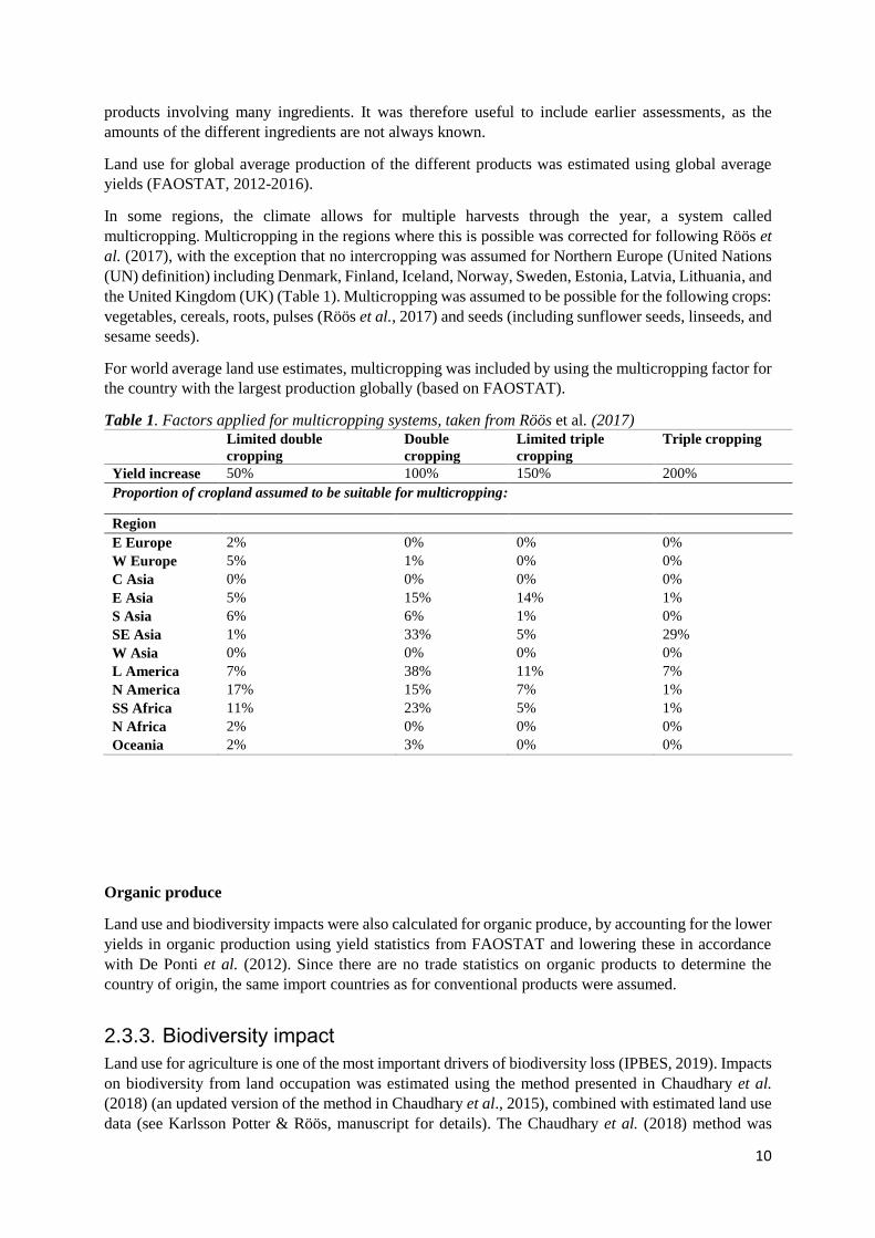
In some regions, the climate allows for multiple harvests through the year, a system called

multicropping. Multicropping in the regions where this is possible was corrected for following Röös et

al. (2017), with the exception that no intercropping was assumed for Northern Europe (United Nations

(UN) definition) including Denmark, Finland, Iceland, Norway, Sweden, Estonia, Latvia, Lithuania, and

the United Kingdom (UK) (Table 1). Multicropping was assumed to be possible for the following crops:

vegetables, cereals, roots, pulses (Röös et al., 2017) and seeds (including sunflower seeds, linseeds, and

sesame seeds).

For world average land use estimates, multicropping was included by using the multicropping factor for

the country with the largest production globally (based on FAOSTAT).

Table 1. Factors applied for multicropping systems, taken from Röös et al. (2017) Limited double

cropping

Double

cropping

Limited triple

cropping

Triple cropping

Yield increase 50% 100% 150% 200%

Proportion of cropland assumed to be suitable for multicropping:

Region

E Europe 2% 0% 0% 0%

W Europe 5% 1% 0% 0%

C Asia 0% 0% 0% 0%

E Asia 5% 15% 14% 1%

S Asia 6% 6% 1% 0%

SE Asia 1% 33% 5% 29%

W Asia 0% 0% 0% 0%

L America 7% 38% 11% 7%

N America 17% 15% 7% 1%

SS Africa 11% 23% 5% 1%

N Africa 2% 0% 0% 0%

Oceania 2% 3% 0% 0%

Organic produce

Land use and biodiversity impacts were also calculated for organic produce, by accounting for the lower

yields in organic production using yield statistics from FAOSTAT and lowering these in accordance

with De Ponti et al. (2012). Since there are no trade statistics on organic products to determine the

country of origin, the same import countries as for conventional products were assumed.

2.3.3. Biodiversity impact

Land use for agriculture is one of the most important drivers of biodiversity loss (IPBES, 2019). Impacts

on biodiversity from land occupation was estimated using the method presented in Chaudhary et al.

(2018) (an updated version of the method in Chaudhary et al., 2015), combined with estimated land use

data (see Karlsson Potter & Röös, manuscript for details). The Chaudhary et al. (2018) method was

11

chosen since it was the most recent method and represents an improvement on earlier methods to account

for biodiversity impacts in LCA (de Baan et al., 2012). It is also the method recommended by the United

Nations Environment Programme-Society of Environmental Toxicology and Chemistry (UNEP-

SETAC) for assessing biodiversity impacts from agriculture (UNEP, 2019). The method provides a

global characterization factor, which was required in the present context, and allows for distinction

between different land use types, although these are still rather broad. The method uses country area

species richness (SAR), which is a model for estimating, based on available data, species richness

(number of species) for different taxa (such as mammals and plants) in different land use types,

compared with the natural habitat (Chaudhary et al., 2018). The method also incorporates a vulnerability

score that takes the presence and range of endangered species into account (Chaudhary et al., 2018).

Impact on species richness in five different taxa is included: mammals, birds, amphibians, reptiles, and

plants (notably leaving out e.g., insects) and five different land use types: natural habitat, regeneration

secondary vegetation, managed forests, plantation forests, crop land, and urban land, the latter four with

three different intensity levels (minimal, light, and intensive) (Chaudhary et al., 2018). In the present

analysis, land use intensity was assumed to be cropland-intensive use for conventional farming and

cropland-light use for organic production. The taxa-aggregated characterization factors for land

occupation were used.

2.3.4. Water use

Food production is one of the most water-demanding sectors globally, with around 70% of all freshwater

use estimated to be in agriculture (FAO, 2017).

The environmental assessment of water use was based on total water use (as an indicator of water use

as an resource demand), blue water use (as an indicator of freshwater use), and potential impacts on

local water stress, assessed by the AWARE method (explained below).

Data on total water use (green, blue, and grey water) and blue (fresh) water use were collected from

Mekonnen et al. (2011). Figure 1 illustrates water types included in green and blue water (Hoekstra et

al., 2011). Green water is the precipitation on land that does not run off or recharge the groundwater,

i.e., water that is (temporarily) stored in the soil and will eventually be taken up by plants or evaporate

(Hoekstra et al., 2011). The green water use reported in Mekonnen et al. (2011) corresponds to the

rainwater consumed during crop production. Blue water is surface or fresh water consumed during crop

production, i.e., irrigation water that is evaporated from the field or taken up by plants (Hoekstra et al.,

2011). Grey water is the theoretical amount of water needed to dilute pollutants and nutrients leaching

from the field (Hoekstra et al., 2011). Due to lack of data, only nitrogen leaching was considered by

Mekonnen et al. (2011) when estimating the amount of grey water, and hence also in this study.

12

Figure 1. Description of green and blue water, taken from Hoekstra et al. (2011). Evapotranspiration

= evaporation and transpiration by plants.

Water use for processing was included for ready-made protein sources (Appendix A2) and plant-based

dairy replacements (Appendix A3). Water use for washing e.g., vegetables was not included.

AWARE

The water footprint scarcity method AWARE (Available Water Remaining) was used to assess local

(country-level) impacts from water consumption (blue water use) (Boulay et al., 2018). Methods for

assessing freshwater use and the impact on water availability are currently under development for

application in LCA. A well-known earlier method, developed by Pfister et al. (2009), is primarily based

on withdrawal in relation to availability, i.e., human use of freshwater. The AWARE method is based

on demand in relation to availability, meaning that both ecosystem and human demands are accounted

for (Boulay et al., 2018). On analyzing the methods of Pfister et al. (2009) and Boulay et al. (2018),

Lundmark (2019) found that the results differed somewhat, but that the ranking of the products, i.e., the

best to worst performing products, was largely similar. The AWARE method (Boulay et al., 2018) was

selected here because it builds on consensus by the working group on Water Use in Life Cycle

Assessment (WULCA) under the UNEP-SETAC Life Cycle Initiative (Boulay et al., 2018). It is

currently the recommended method for water scarcity assessment in LCA, but it is also recommended

that a complementary method be used for sensitivity analysis (Jolliet et al., 2018). Sensitivity analysis

of the results in this report is described by Lundmark (2019).

The AWARE method offers yearly average characterization factors and country average factors for

agricultural land and unspecified land for different countries. Characterization factors are also given on

watershed level, which would be preferable (over country average) for assessing the impact on water

stress. Similarly, there are temporal differences in the effect of freshwater use on water scarcity (Boulay

et al., 2018). However, since geographical location and time of crop production were not known for all

crops assessed, we used country average characterization factors for agricultural land.

2.3.5. Pesticide use

Estimating the impact of pesticide use in food production is challenging. This is mainly due to lack of

data on pesticide use (especially divided into different food products) and limitations in methods to

assess eco-toxicity and human toxicity, i.e., the actual negative impacts on ecosystems and humans, for

the vast number of pesticides on the market. To compare all products on the Swedish market, statistics

13

on pesticide use for all countries exporting to Sweden would be needed. No such data are currently

available, especially for countries outside the EU, for which data on pesticide use are very scarce.

In this report, statistics on pesticide use based on the amount of active substance (kg AS) per hectare, in

Sweden and Europe (only for EU member states), are presented. These data can give an indication of

the ecotoxicity impacts from the production of different crops. The most recent statistics on EU pesticide

use do not include data for individual crops, but give aggregated figures for the whole country. For

European products, an publication from 2007 was therefore used (EUROSTAT, 2007). It presents

average (1999-2003) pesticide use for different European countries for “cereals, maize, oil seeds,

potatoes, sugar beet, other arable crops (arable crops total), fruit trees, vegetables (fruit and vegetables

total)”. The most recent available statistics were used for Swedish products (SBA, 2018b).

For imports from outside Europe, no uniform dataset could be found for pesticide use in different crops

in different countries. Therefore, no data on pesticide use were collected for production outside Europe.

In the Vego-guide, this was treated as “lack of data”, similarly to European and Swedish production for

which no data could be found. See Karlsson Potter and Röös (manuscript) for more details on how this

was handled in the Vego-guide.

Results from data collection on pesticide use, aggregated for all food categories, are presented in Chapter

3 of this report. Detailed data for all food products are presented in Appendix A7.

2.4. Functional unit and system boundaries

The functional unit (FU) selected was 1 kg product at a store in Sweden, i.e., the following steps in the

production chain were included: primary production including the production of inputs, processing (in

the case of processed products), storage, packaging, and transport to a store in Sweden.

There are several alternatives to using a mass-based functional unit. For food products, the functional

unit could be e.g., protein content for protein foods, energy content for carbohydrate sources, or based

on different nutrient indices. This issue is further discussed in Appendix A4.

The functional unit when collecting data from earlier studies was 1 kg product, and studies with varying

system boundaries were included. To enable us to compare the results from earlier studies, the results

were modified to represent the same system boundary. This meant that if e.g., cooking and waste

management were included in the study, these steps were removed. For studies that ended at factory

gate/farm gate, emissions from transport to a retailer (in Sweden) were added. More detailed information

about this can be found in Appendix A1.

Emissions from transport and packaging were added using emission factors from Moberg et al. (2019)

(Tables 2 and 3). In general, all transport was considered to be road and/or sea transport. Transport

within Sweden was also included for both imported and domestic products. Transport within Sweden

was calculated using weighted average for food transport within Sweden, meaning that population

distribution was accounted for (Moberg et al., 2019).

For packaging, representative packaging type was considered for the different products in Table 3, after

analysis by Moberg et al. (2019). The climate impact for packaging used is well in line with the climate

impact of different packaging types presented by Nilsson et al. (2009), with the exception of metal cans

and glass jars. This because no such packaging was assumed for the products included. Beans sold as

ready-to eat in Sweden today are mainly packaged in cardboard cartons (see Appendix A6). However,

it is important to note that the climate impact from transport and packaging was considered using rather

general figures, i.e., no specific analysis of transportation mode and typical packaging type was made

for each product.

14

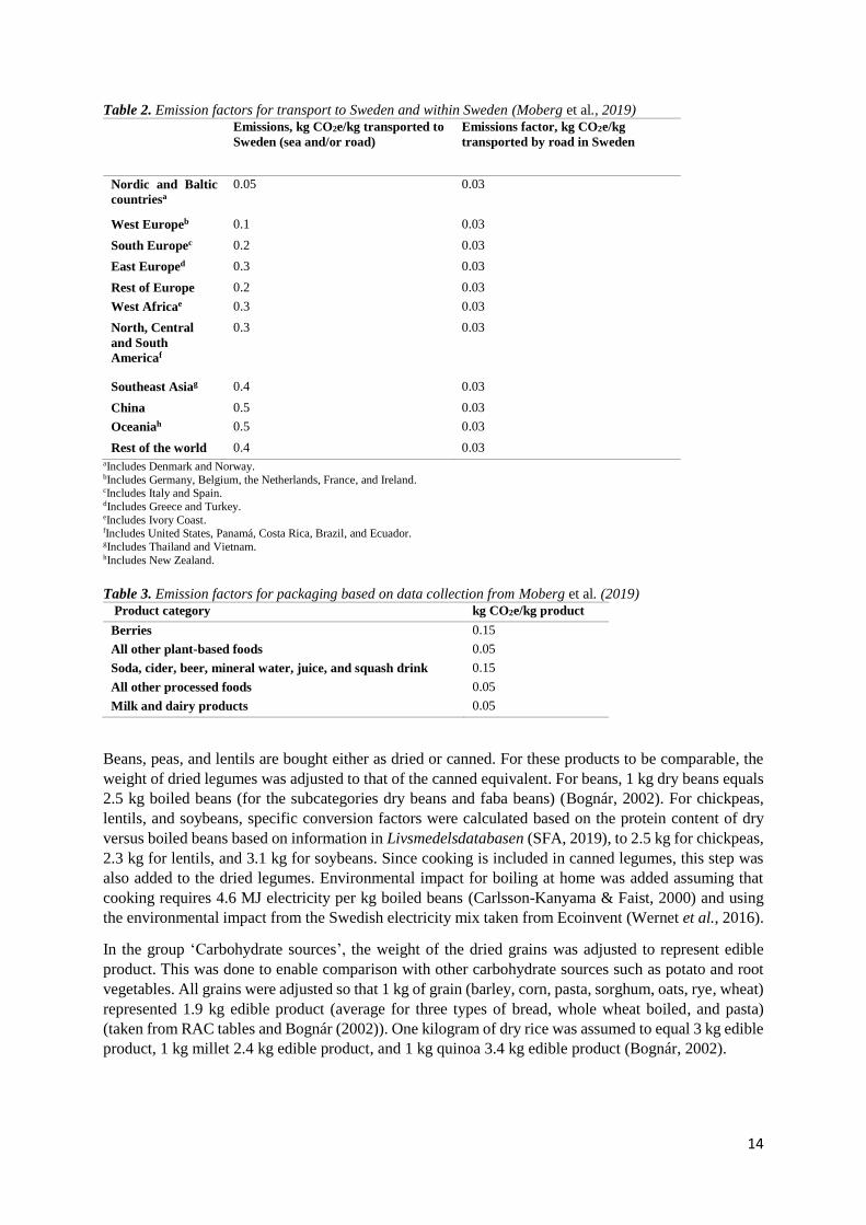
Table 2. Emission factors for transport to Sweden and within Sweden (Moberg et al., 2019) Emissions, kg CO2e/kg transported to

Sweden (sea and/or road)

Emissions factor, kg CO2e/kg

transported by road in Sweden

Nordic and Baltic

countriesa

0.05 0.03

West Europeb 0.1 0.03

South Europec 0.2 0.03

East Europed 0.3 0.03

Rest of Europe 0.2 0.03

West Africae 0.3 0.03

North, Central

and South

Americaf

0.3 0.03

Southeast Asiag 0.4 0.03

China 0.5 0.03

Oceaniah 0.5 0.03

Rest of the world 0.4 0.03 aIncludes Denmark and Norway. bIncludes Germany, Belgium, the Netherlands, France, and Ireland. cIncludes Italy and Spain. dIncludes Greece and Turkey. eIncludes Ivory Coast. fIncludes United States, Panamá, Costa Rica, Brazil, and Ecuador. gIncludes Thailand and Vietnam. hIncludes New Zealand.

Table 3. Emission factors for packaging based on data collection from Moberg et al. (2019)

Product category kg CO2e/kg product

Berries 0.15

All other plant-based foods 0.05

Soda, cider, beer, mineral water, juice, and squash drink 0.15

All other processed foods 0.05

Milk and dairy products 0.05

Beans, peas, and lentils are bought either as dried or canned. For these products to be comparable, the

weight of dried legumes was adjusted to that of the canned equivalent. For beans, 1 kg dry beans equals

2.5 kg boiled beans (for the subcategories dry beans and faba beans) (Bognár, 2002). For chickpeas,

lentils, and soybeans, specific conversion factors were calculated based on the protein content of dry

versus boiled beans based on information in Livsmedelsdatabasen (SFA, 2019), to 2.5 kg for chickpeas,

2.3 kg for lentils, and 3.1 kg for soybeans. Since cooking is included in canned legumes, this step was

also added to the dried legumes. Environmental impact for boiling at home was added assuming that

cooking requires 4.6 MJ electricity per kg boiled beans (Carlsson-Kanyama & Faist, 2000) and using

the environmental impact from the Swedish electricity mix taken from Ecoinvent (Wernet et al., 2016).

In the group ‘Carbohydrate sources’, the weight of the dried grains was adjusted to represent edible

product. This was done to enable comparison with other carbohydrate sources such as potato and root

vegetables. All grains were adjusted so that 1 kg of grain (barley, corn, pasta, sorghum, oats, rye, wheat)

represented 1.9 kg edible product (average for three types of bread, whole wheat boiled, and pasta)

(taken from RAC tables and Bognár (2002)). One kilogram of dry rice was assumed to equal 3 kg edible

product, 1 kg millet 2.4 kg edible product, and 1 kg quinoa 3.4 kg edible product (Bognár, 2002).

15

2.5. Food products and food groups

The food products were divided into the following food categories: Protein sources, Plant-based drinks

and cream, Carbohydrate sources, Nuts and seeds, Fruits and berries, and Vegetables and mushrooms.

The Vego-guide aims to include the main plant-based commodities on the Swedish market, including

plant-based protein sources and other products such as nuts that are interesting for many consumers

choosing to eat less animal-based products, and which are relevant for a more plant-based diet. The list

of products assessed was continuously discussed with WWF Sweden.

Some products were excluded due to lack of data. For example, the aim was to include more variants of

plant-based protein sources, but this was not possible due to lack of data. Similarly, there are few studies

on different types of mushrooms and it was therefore decided to provide data only for Agaricus bisporus

(common mushroom, champinjon in Swedish).

Table 4. Food categories and food products included in the analysis, but not necessarily in the final

guide Protein

sources

Carbohydrate

sources

Plant-based drinks

and cream

Fruit and

berries

Vegetables and

mushrooms

Green peas Cereals Almond drink Apples Artichokes

Yellow peas Barley Coconut drink Apricots Asparagus

Dry beans Maize Soy drink Bananas Avocados

Faba beans Millet Oat drink Cherries Broccoli

Canned beans (including Oats Oat cream Dates Cabbage

lentils) Pasta Coconut milk Grapefruit and Capsicums/

Chickpeas Quinoa pomelo Peppers

Dry lentils Rice Grapes Cauliflower

Soybeans Rye Guavas and mangoes Celery

Ready-made products Sorghum Kiwi fruit Cucumber

Mixed without animal Wheat Lemons and limes Eggplant

products1 Root vegetables Melons Garlic

Pea-protein products Beetroot Oranges Ginger

Quorn Carrots Papayas Lettuce

Soy-based Potatoes Peaches Green beans

Tofu and tempeh Swedes Pears Olives

Nuts and seeds Sweet potato Pineapples Onions

Almonds Jerusalem artichoke Plums and sloes Pumpkins and

Cashew nuts Parsnips Tangerines, squash

Chestnuts mandarins etc. Spinach

Coconut (grated) Watermelon Tomatoes

Hazelnuts Berries Mushrooms

Walnuts Cranberries

Pistachios Blueberries

Peanuts Raspberries and

Sesame seeds other berries

Sunflower seeds Strawberries 1For example falafel.

2.6. Strategy used for producing final estimates for the Vego-

guide

Here we describe the method used for analyzing the data and arriving at likely impact, or range of

impact, of the specific product on the Swedish market.

Climate impact

16

The final assessments on the climate impact of different products were based on the results from the

literature review of earlier studies and an analysis of the applicability of the results for products found

on the Swedish market. This analysis was based on information regarding countries that export to

Sweden and how representative the study was of current production systems including technological

developments. For many products, there were a limited number of studies available. In these cases,

available earlier studies were used to give an indication of possible climate impact. After each final

assessment in tables in this report, the number of references used for making the final assessment for

each individual product is shown. The sources included scientific papers, reports, databases, and in some

cases company documents. We compiled the results from previous studies and expressed the likely

climate impact in terms of “likely below X kg CO2e per kg product”, where the relevant study with the

highest climate impact was used to describe the climate impact that the particular product will most

likely not exceed (since all other identified studies showed a lower climate impact). For most products,

relatively few studies were identified and it was therefore not considered feasible to use an average value

of the studies found.

Land use, biodiversity, and water use (including water scarcity indicator)

Final assessments for land use, biodiversity and water use (see Chapter 3) were primarily based on

assessments performed within this study (see section 2.3.2, 2.3.3, 2.3.4). For the product groups ‘Protein

sources’ and ‘Plant-based drinks and cream’, results from earlier studies were used in the final

assessment, because these groups contain ready-made products with several processed ingredients and

therefore information from previous studies is particularly relevant. Swedish production, production in

the countries identified as main exporters to Sweden, and global average production were included. In

the final assessments, we describe the range of land use and water use for the production regions. We

also state whether the results are homogenous or heterogeneous, and discuss the reasons. For impact on

biodiversity and water scarcity, we discuss the products that risk having the largest impact on these

parameters.

17

3. RESULTS: FOOD CATEGORIES

This chapter presents a summary of the results of data collection for the different food groups and

products. More details on individual earlier studies that formed the basis for the climate impact

assessment can be found in Appendix A1.

Below, the results from earlier studies and from the assessments performed in the present analysis are

presented for the impact categories climate impact, land use, biodiversity impact, and water use for all

six product groups. Lastly, pesticide use is presented separately for all product groups under one

heading, because only aggregated results are presented in this report. Detailed results for all products

are presented in Appendix A7.

3.1. Protein sources

Note that the environmental impact of dry legumes was modified to be comparable with canned legumes

and ready-to-eat meat alternatives (see section 2.4). Results that were modified in this way are marked

with * in diagrams. This means that the protein content in the legume-based product is approximately

7-8%. For many of the meat replacement products, such as soy-based “meat”, the protein content is

more similar to that of meat (approximately 20%).

For ready-made products, the symbol in graphs representing the region of origin shows country of

processing. This means that soy-based products produced in e.g., Sweden will be listed as Swedish even

though ingredients are imported.

3.1.1. Climate impact

Results for climate impact from earlier studies on plant-based protein sources are presented in Figure 2.

Most studies on unprocessed beans and peas show a climate impact below 1 kg CO2e per kg product.

However, there are some exceptions: a study on green peas produced in Australia and transported to

Sweden (which is unlikely for fresh green peas in practice), and the following data-points, all from the

databases of ecoinvent (Wernet et al., 2016) and Agri-footprint (Agri-footprint, 2018), where LUC is

included: yellow peas from Spain, chickpeas from Australia, and several studies on soybeans produced

in South America (Argentina and Brazil). Australia is the country with the largest export of chickpeas

and therefore chickpeas from Australia could potentially be relevant for the Swedish market

(FAOSTAT, 2019). Note that no dry or canned chickpeas from Australia were found in the main

supermarkets in Sweden during an inventory performed in 2019 (Ekqvist et al., 2019). However,

soybeans from Brazil and Argentina are interesting to take into consideration, as these countries are

major producers of soybeans, although they were not identified as countries exporting to Sweden in this

study. It has been estimated that soybeans produced in South America are rarely used for human

consumption in the EU, since they are often GM soybeans and therefore unlikely to be used for human

consumption in the EU (Fraanje & Garnet, 2020). Soybeans have multiple uses, including direct human

consumption, vegetable oil production for human consumption and biofuel production, and animal feed

production. It has been estimated that around 6% of total soybean production is used directly for human

consumption, most of the oil and a small fraction (less than 1%) of the protein press cake (a co-product

from oil pressing) is used for human consumption, and most of the global soybean production is used

for animal feed, primarily for poultry and pork production (Fraanje & Garnet, 2020).

18

Dry lentils have a climate impact of between 0.9 and 2.6 kg CO2e per kg product (including transport to

Sweden) for lentils produced in Australia, Iran, and Canada. Lentils from Australia have the highest

climate impact, as mainly due to LUC (Agri-footprint, 2018). Data for Iranian and Australian lentils

were not considered relevant for the Swedish market. The main countries from which Sweden imports

lentils were found to be Turkey, UK, and Canada (Canada being the largest producer globally, and

identified as the largest exporter) (FAOSTAT, 2019). Ekqvist et al. (2019) found that most lentils on

the Swedish market come from Canada. Therefore, data for Canadian lentils were used as the basis for

the final assessment.

For canned beans, chickpeas, and lentils, some studies show impacts exceeding 1 kg CO2e per kg

product. It is unclear from these studies whether metal or cardboard packaging was used, as this has an

impact on the results. However, the electricity mix in the country where the beans are boiled, and the

fact that more weight has to be transported to Sweden if the beans are boiled before transport, are clearly

important for the final climate impact. An assessment of the climate impact of canned beans produced

in Italy and of dry beans transported and boiled at home in Sweden is presented in Appendix A6.

Currently, there is no facility in Sweden producing canned beans, and beans grown in Sweden and sold

as canned beans in Sweden are likely to have been canned in Italy (Tidåker et al., manuscript).

For ready-made plant-based protein sources, such as soy-based mince, sausages, etc., most studies show

a climate impact of 1-4 kg CO2e per kg product. However, some studies show an even higher impact.

One study on dairy-based protein (Broekema & Blonk, 2009) shows a climate impact of just below 6 kg

CO2e per kg product. This is an animal-based product of a type that is currently not very common on

the Swedish market. Mixed (especially mixed with eggs) products have very diverse impacts, due to the

diversity of ingredients in these products. All products that show an impact higher than 4 kg CO2e per

kg product are products with eggs produced in the USA (Quantis, 2016) and assumed to be transported

to Sweden. These products are, to our knowledge, not available on the Swedish market.

Studies on Quorn often report a climate impact of between 2-3 kg CO2e per kg product (Louise

Needham, Quorn, personal communication 2019). Blonk et al. (2008), Head et al. (2011), Broekema

and Blonk (2009), and Finnigan et al. (2010) found a higher impact, of around 7 kg CO2e per kg product,

for Quorn. Finnigan et al. (2010) report a higher impact from processing than e.g., Blonk et al. (2008),

but the impact from raw materials is similar in the two studies. Later studies on Quorn by the same

author show a lower impact (Finnigan et al., 2017). The later studies were considered in the

recommendation in this report, since the company producing Quorn has modified its process to lower

the climate impact (Louise Needham, personal communication 2017).

Soy-based products show an impact of 1-3 kg CO2e per kg product. In particular, products partly

produced in Sweden have a low impact, likely due to the low climate impact of Swedish electricity

production. Two studies show an impact above 4 kg CO2e per kg product, both for products produced

in the USA (Quantis, 2016) and transported to Sweden. Tofu and tempeh likely have an impact lower

than 3 kg CO2e per kg product (range 1-4 kg CO2e per kg product, the higher range of impact was not

considered in the recommendation due to the large discrepancies with the other studies) (Table 5). Very

few studies were found on wheat protein-based products. The results in Figure 2 show results from one

study (Broekema & Blonk, 2009) for wheat protein, and not the finished (ready-to-eat) product.

No studies were found on processed products produced from Swedish ingredients, such as tempeh made

from peas or faba beans. Our judgment is that the climate impact is lower than for imported products,

as transportation is shorter and the Swedish electricity mix has a low climate impact, giving a low impact

from the processing step.

19

Figure 2. Climate impact of plant-based protein sources. Functional unit 1 kg packaged product at a Swedish

retailer. *Weight of the product modified to equal 1 kg boiled beans and climate impact from cooking added. Note

that the graph shows the climate impact from all identified earlier studies for this product group, and not only

those identified as relevant for the Swedish market. The final assessment (see Table 5) was based on relevance for

the Swedish market.

Table 5. Summary of assessments of the climate impact of plant-based protein sources on the Swedish market Product Final assessment

(kg CO2e per kg

product in a

Swedish store)

No. of

relevant

references

Total no.

of

references

Comment

General Sweden

Green peas 0.8 No data 3 4 Only European produce considered relevant

Yellow peas 0.5 0.3 7 (5 SW) 8 Only European produce considered relevant, Agri-

footprint data from Spain excluded due to relatively

high LUC impact. Spain was not identified as one of

the countries exporting yellow peas to Sweden.

Dry beans 0.7 0.4 7 (4 SW) 7 All studies considered relevant for the general

recommendation. Three studies on Swedish beans

were found, showing an impact below 0.4 kg CO2e per

kg.

Faba beans 0.5 0.2 3 (1 SW) 3 All studies considered relevant. The higher impact is

for faba beans from Australia, dominated by emissions

from transportation and land use change. Only one

study was found on Swedish faba beans, so this

assessment is uncertain.

Canned

legumes

1.7 No data 4 4 All studies considered relevant. No data on Swedish

canned beans found. Climate impact today is likely to

be lower, since many beans are sold in cardboard

containers (Tetra PakTM) and many of the identified

studies considered tin cans.

Chickpeas 0.6 No data 3 3 All studies considered relevant. Data for Australian

chickpeas excluded due to high LUC and questionable

relevance for the Swedish market.

Dry lentils 0.6 0.2 2 (1 SW) 3 Data for lentils from Canada, Australia, and Sweden

considered relevant for the Swedish market.

Assessments for imported and Swedish lentils are both

20

based on only one reference, so this assessment is

considered relatively uncertain.

Soybeans 0.6 No data 4 4 Data for soybeans from Brazil and Argentina excluded

due to high LUC impact and these countries not being

identified as important exporters of soybeans for

human consumption to Sweden. They are important

producers globally, and it should be noted that

soybeans can be associated with high LUC impacts.

Processed

Mixed

without

animal

products

2.6 1 4 (1 SW) 5 Data on products produced in Europe and Sweden

considered relevant. Swedish-produced falafel has an

impact well below 1 kg CO2e per kg product. Only data

on products produced in the USA were available for

production outside Europe, and were considered less

relevant for the Swedish market.

Mixed with

animal

products

2.6 1.4 3 (1 SW) 4 Data on products produced in Europe and Sweden

considered in the assessment. Only data on product

produced in the USA were available for production

outside Europe, and were considered less relevant for

the Swedish market.

Pea-protein

products

2.2 No data 1 1 Only one study of European-produced (German) pea-

protein product was found, so the data should be

considered uncertain.

Quorn 2.7 No data 4 5 Data on European Quorn production considered

relevant. One older study was identified showing a

significantly higher climate impact per kg product.

This study was not considered in the assessment, since

it has been updated with newer studies.

Soy-based 2.2 2.2 3 (2 SW) 5

Data for soy protein isolates (that cannot be eaten as is

but is processed into other products) and data on US

production were considered less relevant for the

Swedish market. One study showed an impact of 3.1

kg CO2e per kg. However, this was excluded due to

deviation from the other identified studies.

Tofu and

tempeh

2.3 No data 4 5 All data considered relevant for the assessment. Most

studies show a climate impact below 2.3 kg CO2e per

kg product. One study showed an impact of above 3 kg

CO2e per kg product. This was not considered in the

assessment due to its deviation from the other

identified studies. For Swedish-produced products

such as tempeh made from peas or faba beans, the

climate impact is likely to be somewhat lower than for

similar imported products.

Wheat

protein

1.3 No data 1 1 Only one study was identified, the assessment is

therefore uncertain.

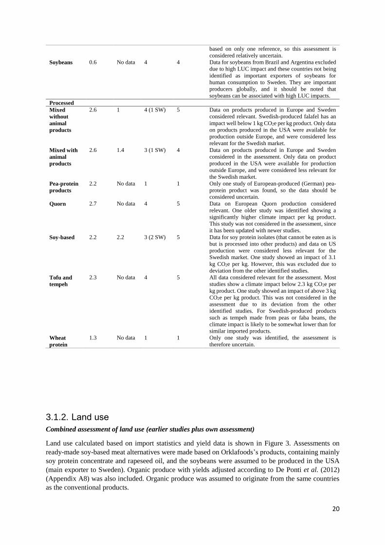
3.1.2. Land use

Combined assessment of land use (earlier studies plus own assessment)

Land use calculated based on import statistics and yield data is shown in Figure 3. Assessments on

ready-made soy-based meat alternatives were made based on Orklafoods’s products, containing mainly

soy protein concentrate and rapeseed oil, and the soybeans were assumed to be produced in the USA

(main exporter to Sweden). Organic produce with yields adjusted according to De Ponti et al. (2012)

(Appendix A8) was also included. Organic produce was assumed to originate from the same countries

as the conventional products.

21

Yellow peas, faba beans, soybeans, Quorn (made from wheat-based sugar), and ready-made vegetarian

meat alternatives based on mainly soy protein concentrate were found to have relatively low land use

(mainly below 2 m2 per kg product). All literature data-points on soy-based European products are from

the same study (blonkconsultans, 2017), in which land use values for the products covered are higher

than the land use calculated here for Swedish products. This can be partly be due to South American

soybeans being assumed in blonkconsultans (2017), whereas for Swedish ready-made soy-based meat

alternatives the beans were assumed to come from the USA, which has higher yields (FAOSTAT, 2019).

However, this cannot explain the whole difference. One identified study (Thrane et al., 2017) looking

at soy protein isolate production in the US was not included in the assessment, as soy protein isolate has

a very high protein content and is further processed into products containing much lower protein content.

Comparison to ready-to-eat products is therefore not relevant.

Results from existing studies (Figure 3) show that ready-made meat alternatives have higher land use

than unprocessed legumes per kg. The reason for this is that ready-made products often contain other

ingredients than legumes, such as oil, seeds, or nuts. Tofu is often produced from soybean, but fractions

of the bean are removed from the products (in this case fibers and some of the carbohydrates). For

products such as tofu, the results for land use will depend partly on how the land use is allocated between

the different fractions in the processing. Quorn, with the primary input of glucose (produced from

wheat), is an exception, with low land use due to high sugar yield per hectare. Soy-based meat

alternatives made primarily from soy-protein concentrate also show low land requirements.

Figure 3. Land use for plant-based protein sources in m2/year per kg ready-to-eat product. Earlier studies and

own assessments on land use are shown. *Weight of the product modified to equal 1 kg boiled beans. World

average land use is based on average yield for all countries that produce the crop.

For reference, land use for all plant-based products (same as in Figure 3) and meat (bone-free meat) is

presented in Figure 4. Land use data for meat were taken from Röös et al. (2013, 2015). Two data points

show land use of above 150 m2 per kg beef (Röös et al., 2013), but these were removed from the graph

to enable more details to be shown. Both beef and pork clearly have a much higher land use than

22

vegetable protein source. Chicken is in the same range as the vegetable protein sources with relatively

high land use, but more than double the land use of most European soy-based products.

Figure 4. Land use for vegetable protein sources and meat in m2/year per kg product. *Weight of the product

modified to equal 1 kg boiled beans. Note that land use for beef is to varying extents grazing land, and therefore

direct comparison to cropland-based products, including plant-based protein sources, pork, and chicken, is

difficult.

3.1.3. Biodiversity impact

Products with relatively high land use and that are imported from countries with high biodiversity such

as Lebanon (faba beans) have a high impact on biodiversity. Legumes from the south of Europe, e.g.,

lentils from Italy, tend to have a higher impact on biodiversity than Swedish produce.

Organic produce has a higher biodiversity impact for all crops assessed, due to higher land use. The

lower factor for lower-intensity agriculture in Chaudhary et al. (2018) does not compensate for the lower

yield of organic produce. However, Chaudhary et al. (2018) present gross factors, so this should be

interpreted with great care.

Biodiversity impact for Quorn, tofu, and tempeh was calculated using land use data from earlier studies

(Figure 3) and by attributing all that land use to the main ingredient in the respective product (glucose

from wheat for Quorn, soybeans for tofu and tempeh).

23

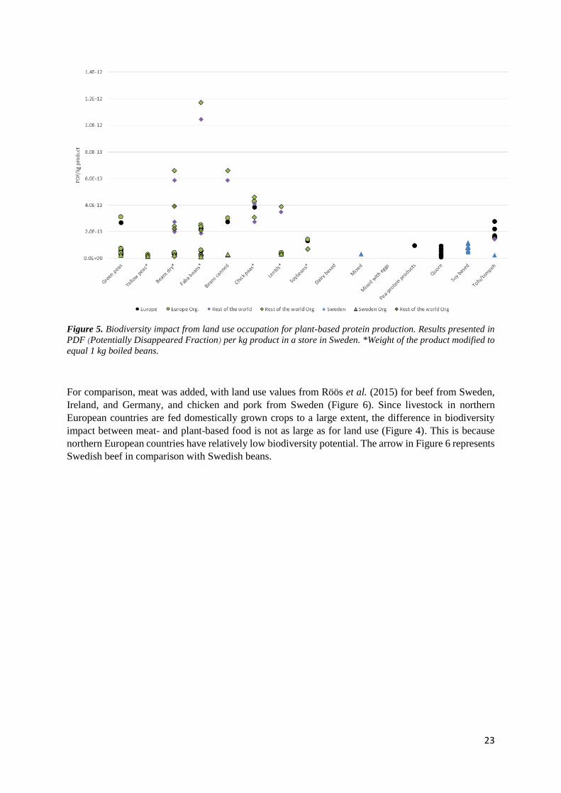
Figure 5. Biodiversity impact from land use occupation for plant-based protein production. Results presented in

PDF (Potentially Disappeared Fraction) per kg product in a store in Sweden. *Weight of the product modified to

equal 1 kg boiled beans.

For comparison, meat was added, with land use values from Röös et al. (2015) for beef from Sweden,

Ireland, and Germany, and chicken and pork from Sweden (Figure 6). Since livestock in northern

European countries are fed domestically grown crops to a large extent, the difference in biodiversity

impact between meat- and plant-based food is not as large as for land use (Figure 4). This is because

northern European countries have relatively low biodiversity potential. The arrow in Figure 6 represents

Swedish beef in comparison with Swedish beans.

24

Figure 6. Biodiversity impact from land use occupation by vegetable protein production and meat production.

Results in PDF (Potentially Disappeared Fraction) per kg product. *Weight of the product modified to equal 1 kg

boiled beans.

Table 6. Range of results for all identified export countries and Swedish produce for land use (m2/year per

functional unit (FU)) and biodiversity impact (Potentially Disappeared Fraction (PDF) per FU) for plant-based

protein sources

Product Land use

(m2/year per

FU)

Biodiversity

impact (PDF per

FU)

Comment

Green peas 1.1-2.7 2.1E-14-3.1E-13 Green peas from Sweden, the Netherlands, and Italy have land use of around

2-2.7 m2 per kg. For all other countries assessed and global average, land use

is below 2 m2 per kg for both conventional and organic.

Yellow peas 0.9-1.6 1.2E-14-2.7E-14 For all export countries assessed, global average and Swedish production

land use is below 1.6 m2 per kg.

Dry beans 1.3-5.4 1.3E-14-6.6E-13 For all export countries assessed except Argentina, land use is below 3 m2

per kg. World average land use is significantly higher, which indicates a risk

of higher land use in other export countries.

Faba beans 1.1-6.5 1.1E-14-1.2E-12 Land use for imports was assessed to be 1.1-6.5 m2 per kg. Production from

Lebanon (16% of Swedish import) has the highest land use. Swedish

production has land use of around 1.2-1.4 m2 per kg (lower values for

conventional and higher for organic). The biodiversity assessment showed a

risk that faba beans from Lebanon have a high impact on biodiversity from

land occupation (close to or above 1.22E-12 PDF).

Beans canned 1.6-4.2 2.3E-14-6.6E-13 According to Swedish import statistics, Sweden imports canned beans

mainly from Italy, but the beans could have been processed there (most

likely Italy) and then exported to Sweden, i.e., produced in a different

country. Beans produced in Italy were assessed to have land use of 2.0-2.3

m2 per kg products. World average production has a land use of 3.7-4.2 m2

per kg (lower values for conventional and higher for organic). Due to

uncertainties in import statistics, other countries could be relevant, some of

which are included in the assessments of dried beans. Swedish beans are

likely to have land use of 2.5-2.8 m2 per kg (lower values for conventional

and higher for organic).

Chickpeas 2.8-4.3 2.7E-13-4.6-13 Land use in the export countries assessed and world average varies between

2.8-3.4 (conventional) and 3.2-4.3 (organic) m2 per kg.

25

Lentils 2.2-3.6 3.0E-14-3.9E-13 Land use in the export countries assessed and world average varies between

2.2-3.2 (conventional) and 2.5-3.6 (organic) m2 per kg. Swedish lentils were

assessed to have land use of 3.2-3.6 m2 per kg (lower values for conventional

and higher for organic).

Soybeans 0.8-1.2 6.4E-14-1.4E-13 Soybeans are likely to have land use of around 1 m2 per kg.

Ready-made products

Mixed 0.4-5.2 2.1E-14 Earlier studies on European products show land use of 2.5-5.2 m2 per kg (3

references). The Swedish product in the graph is falafel (imported

ingredients) with land use of 0.4 m2 per kg. Biodiversity impact was assessed

only for falafel where the origin of all ingredients was known.

Mixed with

eggs

2.4-3.4 Earlier studies on European products show land use of 2.4-3.4 m2 per kg (2

references).

Pea-protein

products

4.9 9.4E-14 Only one study was found, showing land use of 4.9m2 per kg (1 reference).

Quorn 0.2-1.7 7.1E-15-6.9E-14 Quorn is likely to have land use of 0.4-1.7 m2 per kg. The higher value in the

graph is from an older study.

Soy-based 0.6-4.9 4.7E-14-1.2E-13 Land use for soy-based products varies greatly, depending on yield of the

soybean (country origin) and other ingredients. Swedish-produced products

are mainly produced from soy protein concentrate from imported

ingredients. Land use for these products is likely to be around 1-1.5 m2 per

kg. Similar European products are likely to have similar land use, the higher

land use in the graph can partly be explained by a different country of origin

for the soybeans.

Tofu/tempeh 1.8-3.5 2.3E-14-2.8E-13 Most studies show land use of around 2 m2 per kg. Swedish tempeh was

estimated to have land use of around 2.5 m2 per kg (4 references).

Wheat protein 1.6 9.4E-14 Only one study was found showing land use of 1.6 m2 per kg.

3.1.4. Water use

Earlier studies

Blue water use for the different products is shown in Figure 7, with one study on Quorn (Finnigan et al.,

2010) removed since a more recent study by the same main author shows much lower results (Finnigan

et al., 2017). In all cases shown, blue water use is below 0.5 m3 per kg product (Figure 7).

26

Figure 7. Blue water use in m3 per kg product from earlier studies. *Weight of the product modified to equal 1 kg

boiled legumes.

Water footprint, total water use, and AWARE

Total water use (green, blue, grey) for pulses, ready-made meat alternatives, and animal products is

shown in Figure 8. Water use for animal products is taken from Mekonnen and Hoekstra (2012) and for

crops from Mekonnen et al. (2011). Note that soy-based and mixed products shown as Swedish products

in the graph (Figure 8) are processed in Sweden, but using raw material from outside Sweden.

Animal products (beef, pork, chicken) have substantially higher total water use. For nearly all products,

green water use dominates and products with high land use (animal products) use much more green

water. For world average production, animal products also use significant amounts of blue water. The

product using the most blue water is irrigated faba beans from Egypt.

Grey water use, calculated as the amount of water needed to dilute the nitrogen fertilizer load to legally

acceptable concentrations, is relatively high for legumes, especially dry beans, lentils, chickpeas and

faba beans (Mekonnen et al., 2011). This is because of the relatively high nitrogen leaching in relation

to the relatively low yield (M. Mekonnen, personal communication 2018). Naturally fixed nitrogen by

legumes was not included in the assessment.

27

Figure 8. Green, blue, and grey water use for the protein sources in m3 per kg product in a store in Sweden for

the identified export countries, and world average water use for comparison.

Total water use (as in Figure 8) with geographical origin of the vegetarian protein sources is shown in

Figure 9.

0 2 4 6 8 10 12 14 16

Belgium

France

World average

Sweden

Belgium

The Netherlands

France

World average

Denmark

The Netherlands

Germany

Canada

World average

Sweden

Turkey

The Netherlands

Myanmar

Canada

China

Argentina (extra country)

Poland (extra country)

World average

Sweden

Australia

Egypt

Lebanon

Turkey

Germany

Australien

World average

Sweden

Italy

Myanmar

World average

Sweden

Turkey

Italy

Australia

World average

Turkey

Canada

World average

Italy

USA

World average

Sweden

Sweden

Sweden

Sweden

Sweden

Sweden

Sweden

Sweden

Sweden

Sweden

Sweden

Sweden

Sweden

Sweden

USA

USA

USA

USA

USA

USA

USA

USA

UK

UK

UK

UK

UK

UK

Beef Sweden

Beef World average

Pork Sweden

Pork World average

Chicken Sweden

Chicken World average

Gre

en p

eas

fro

zen

Gre

en p

eas

fres

hP

eas

dry

*B

ean

s d

ry*

Fava

bea

ns*

Bea

ns

cann

edC

hic

kpea

s*Le

nti

lsd

ry*

Soyb

eans

*So

ybas

ed

Mi

xe d

Pe a pr

ote in

Tofu

/tem

peh

Qu

orn

Mea

t

m3/kg product

Green Blue Grey

28

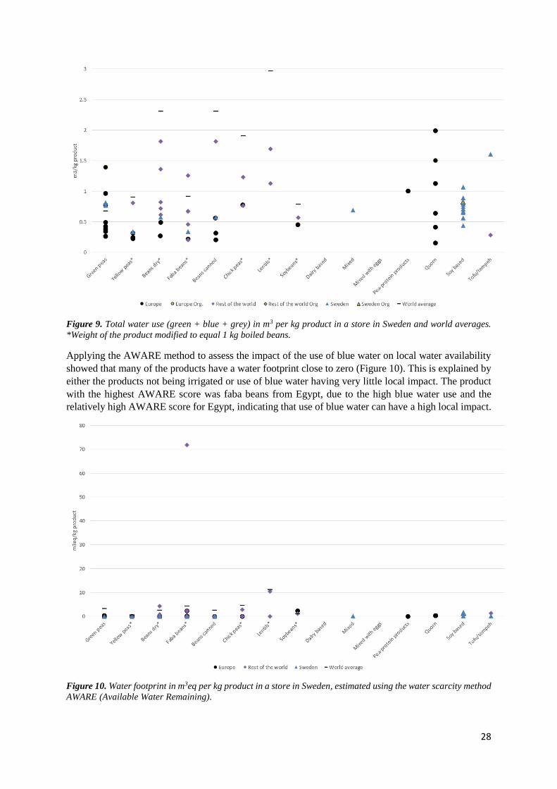
Figure 9. Total water use (green + blue + grey) in m3 per kg product in a store in Sweden and world averages.

*Weight of the product modified to equal 1 kg boiled beans.

Applying the AWARE method to assess the impact of the use of blue water on local water availability

showed that many of the products have a water footprint close to zero (Figure 10). This is explained by

either the products not being irrigated or use of blue water having very little local impact. The product

with the highest AWARE score was faba beans from Egypt, due to the high blue water use and the

relatively high AWARE score for Egypt, indicating that use of blue water can have a high local impact.

Figure 10. Water footprint in m3eq per kg product in a store in Sweden, estimated using the water scarcity method

AWARE (Available Water Remaining).

29

In order to assess animal products using AWARE for comparison, it was assumed that all water use

takes place in the country of origin, i.e., that all fodder is produced in the same country as the meat,

which is a simplification. When including the animal products in the assessment using AWARE, world

average animal products have higher impact than all beans and ready-made vegetarian meat alternatives,

except for faba beans from Egypt (excluded from the diagram to reveal the differences between the other

products) (Figure 11). Swedish meat products have lower impact than some pulses and most of the soy-

based meat alternatives (produced in Sweden, but with raw materials from outside Sweden). However,

the water footprint of Swedish animal products would likely increase if fodder production from outside

Sweden were included, e.g., soybeans from Brazil.

Figure 11. Water footprint in m3eq per kg product in a store in Sweden and world averages using the water

scarcity method AWARE (Available Water Remaining), including animal products. Faba beans from Egypt are

excluded.

Table 7. Range of results for all identified export countries and Swedish produce for total water use (m3 per

functional unit (FU)) and AWARE (Available Water Remaining, m3eq per FU) for plant-based protein sources Product Total water use

(m3 per FU)

AWARE (m3eq

per FU)

Commenta

Green peas 0.3-1.4 0-0.3 Total water use for Swedish production, main export countries, and global

average. AWARE figures do not include world average, since it differs

considerably from the values for Swedish production and the identified

import countries.

Yellow peas 0.2-0.9 0 Yellow peas from Sweden, Denmark, and Germany are likely to have total

water use of below 0.3 m3 per kg product, Canadian and world average

production were assessed to have total water use below 0.9 m3 per kg

product. The AWARE value is zero for all identified export countries, since

yellow peas are generally not irrigated in these countries. The AWARE

figure for global average production is excluded.

Dry beans 0.3-2.3 0-2.3 Swedish, Dutch, Canadian, Argentinean, Polish, and Turkish production has

total water use below 1 m3 per kg product. Beans from China, Myanmar and

world average production have water use above 1 m3 per kg product.

Faba beans 0.2-1.3 0-72 Total water use for faba bean production is mainly below 1 m3 per kg

product, including Swedish production. Except for Egyptian production with

1.3 m3 per kg product. AWARE figures are generally below 4 m3eq, the high

value (72 m3eq) is for Egypt.

30

Beans canned 0.6-2.3 0-2.6 According to Swedish import statistics, Sweden imports canned beans

mainly from Italy and Myanmar, but the beans could have been processed

elsewhere (most likely Italy) and exported to Sweden, i.e., produced in a

different country. Due to uncertainties in import statistics other countries

could be relevant, some of which are included in the assessments of dried

beans. The highest value is for global average production. European

production from Italy and Sweden has the lowest water use.

Chickpeas 0.8-1.9 0-4.7 For total water use, the highest value is for global average production. The

lowest water use is for Italy and Australia.

Lentils 1.1-3.0 0-11 Canada, the world’s largest producer of lentils, has water use of around 1.7

m3 per kg product. No data for Swedish lentil production could be found.

Soybeans 0.5-0.8 1.2-2.2 Water use in the main export countries to Sweden (Italy and USA) is

relatively similar to world average.

Ready-made products Water use for many ready-made products is based on assessments made in

this study, see Appendix A3.

Mixed 0.7 0.07 For falafel, water use is approx. 0.7 m3 per kg product.

Mixed with

eggs

No data.

Pea-protein

products

1.0 0.0002 Water use estimated to be 1 m3 per kg product.

Quorn 0.4-2.0 0.28

Soy-based 0.4-1.1 0.1-1.6 Total water use for soy-based products produced in Sweden from mainly

imported ingredients is 0.4-1.1 m3 per kg product.

Tofu/tempeh 0.3-1.6 0.1-1.3 Total water use was estimated to be 0.3-1.6 0.4-1.2 m3 per kg product.

Wheat protein No data

aComments included when applicable.

3.2. Nuts and seeds

3.2.1. Climate impact

Climate impact for nuts and seeds is presented in Figure 12. Most studies show a climate impact of

below 4 kg CO2e per kg product. The two studies on peanuts that show significantly higher impact (15.6

and 27.3 kg CO2e per kg products) are on peanuts from Uganda and Sudan, respectively. Most of this

impact is from LUC (Agri-footprint, 2018). According to Swedish import statistics, Sweden does not

import peanuts from those two countries (SS, 2018). These two studies were therefore considered to be

of low relevance for the Swedish market and not included in the final assessment (Table 8).

31

Figure 12. Climate impact of nuts and seeds. Functional unit 1 kg nuts and seeds without shells at a Swedish

retailer. A green symbol border indicates that land use change (LUC) is included in the climate impact

assessments. Note that the graph shows the climate impact from all identified earlier studies for this product group,

and not only those identified as relevant for the Swedish market. The final assessment in Table 8 is based on

relevance for the Swedish market.

For almonds, two studies show higher impact than 4 CO2e per kg product, namely the data for the global

market average and “rest of the world” from the ecoinvent database. This is mainly due to energy use

for irrigation (Wernet et al., 2016). Sweden mainly imports almonds from the USA (55%), but also from

Argentina and Spain (SS, 2018). There are several studies on almonds produced in the USA (Kendall &

Brodt, 2014; Marvinney et al., 2014; Venkat, 2012), all showing a climate impact below 4 kg CO2e per

kg product (0.9-2.9 kg CO2e per kg product).

For studies on linseeds, a climate impact lower than 4 kg CO2e per kg product is reported in all but one

case, Agri-footprint data on linseeds from Italy, where the majority of the impact is from LUC (Agri-

footprint, 2018). Around 9% of the linseeds imported to Sweden are from Italy, while the majority come

from Denmark (42%). For pistachios, one study on pistachios from Greece reports a higher impact than

4 kg CO2e per kg product (Bartzas et al., 2017). This could be explained by the functional unit used; in

that study the functional unit was nuts in shell, which was converted here to shelled nuts without

allocating any impact to the shells. Further, the yield in the study by Bartzas et al. (2017) was rather

low. According to trade statistics, Sweden did not import pistachios from Greece during the past five

years (SS, 2018). The data on pistachios from Volpe et al. (2015) are based on Marvinney et al. (2014),

and therefore Volpe et al. (2015) was excluded from the recommendation. For peanuts, two studies show

a higher impact than 4 kg CO2e per kg product, both on peanuts produced in Argentina where direct

LUC is the most important contributor to the climate change impact (Agri-footprint, 2018; Wernet et

al., 2016). According to import statistics, Sweden imports 37% of its peanuts from Argentina (SS, 2018).

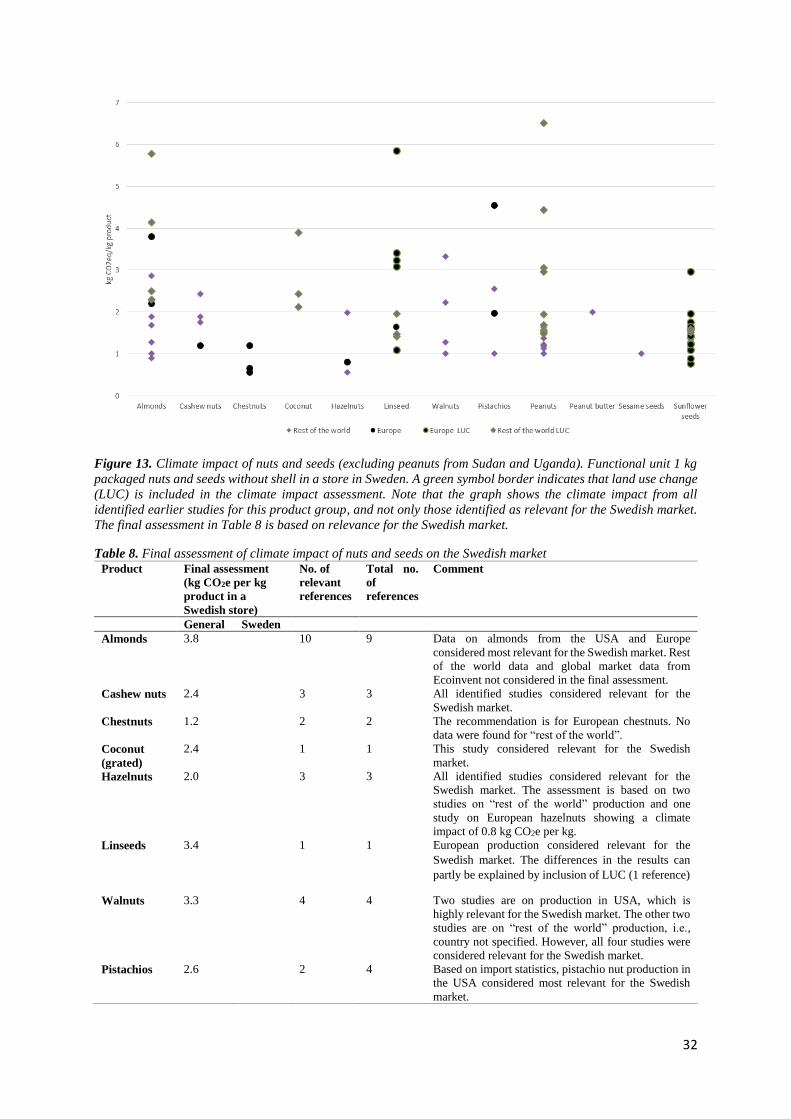
32

Figure 13. Climate impact of nuts and seeds (excluding peanuts from Sudan and Uganda). Functional unit 1 kg

packaged nuts and seeds without shell in a store in Sweden. A green symbol border indicates that land use change

(LUC) is included in the climate impact assessment. Note that the graph shows the climate impact from all

identified earlier studies for this product group, and not only those identified as relevant for the Swedish market.

The final assessment in Table 8 is based on relevance for the Swedish market.

Table 8. Final assessment of climate impact of nuts and seeds on the Swedish market Product Final assessment

(kg CO2e per kg

product in a

Swedish store)

No. of

relevant

references

Total no.

of

references

Comment

General Sweden

Almonds 3.8 10 9 Data on almonds from the USA and Europe

considered most relevant for the Swedish market. Rest

of the world data and global market data from

Ecoinvent not considered in the final assessment.

Cashew nuts 2.4 3 3 All identified studies considered relevant for the

Swedish market.

Chestnuts 1.2 2 2 The recommendation is for European chestnuts. No

data were found for “rest of the world”.

Coconut

(grated)

2.4 1 1 This study considered relevant for the Swedish

market.

Hazelnuts 2.0 3 3 All identified studies considered relevant for the

Swedish market. The assessment is based on two

studies on “rest of the world” production and one

study on European hazelnuts showing a climate

impact of 0.8 kg CO2e per kg.

Linseeds 3.4 1 1 European production considered relevant for the

Swedish market. The differences in the results can

partly be explained by inclusion of LUC (1 reference)

Walnuts 3.3 4 4 Two studies are on production in USA, which is

highly relevant for the Swedish market. The other two

studies are on “rest of the world” production, i.e.,

country not specified. However, all four studies were

considered relevant for the Swedish market.

Pistachios 2.6 2 4 Based on import statistics, pistachio nut production in

the USA considered most relevant for the Swedish

market.

33

Peanuts 1.8 Differences in the results can partly be explained by

inclusion of LUC in some studies. Without LUC, most

studies show a climate impact below 1.8 kg CO2 per

kg product. Climate impact, including LUC of peanuts

from Argentina, Sudan, and Uganda, is likely to be

above 4 kg CO2eq per kg product. Imports from

Argentina are relevant for the Swedish market (6

references).

Sesame seeds 1.0 1 1 The recommendation is based on only one study and

is therefore uncertain.

Sunflower

seeds

1.8 Differences in the results can partly be explained by

inclusion of LUC in some studies. The studies that did

not include LUC show results below 1.8 kg CO2e per

kg product. In total, all but one study show a climate

impact below 2 kg CO2e per kg product, even when

LUC is included (5 references).

3.2.2. Land use

Overall, nuts and seeds were found to have higher land use than the other product groups. This is due to

relatively low yield of shelled nuts and seeds (edible). However, it is important to note that nuts and

seeds are generally high in energy and valuable macro- and micronutrients. This is not reflected in the

results when the functional unit 1 kg product is used. See Appendix A4 for a discussion on functional

unit and the use of nutrient indices.

Earlier studies

Earlier studies provide limited data on land use for nuts and seeds, with the exception of sunflower seeds

and peanuts. The highest land use was found for cashew nuts from production outside Europe (Blonk et

al., 2008). Peanuts from India also show fairly high land use (Wernet et al., 2016).

Figure 14. Land use for nuts (shelled) and seeds from earlier studies, in m2 per kg product.

34

Calculations of land use

Land use for almonds imported to Sweden varies greatly, with notably high land use of above 50 m2 per

kg product for Spanish almonds. Although Spain is a large producer globally, Spanish almond

production has variable yield, and in dry areas and on smaller farms the yield can be low (FAO, year

unknown). Around 10% of the almonds imported to Sweden during the past five years came from Spain

(SS, 2018). Spain is the second largest producer of almonds globally, while the USA is the largest

producer and dominates the global market for almonds (FAOSTAT, 2019). Almond production in the

USA (which accounts for around 55% of Swedish imports) has significantly higher yields (almost six-

fold higher than in Spain) (FAOSTAT, 2019). Italy is another European producer of almonds with fairly

large production globally and Italian yields are 3.6-fold higher than Spanish yields (FAOSTAT, 2019),

indicating that European almond production does not have to be associated with such high land use as

Spanish almond production. Almond production in Turkey and Greece produces similar yields to that

in the USA (FAOSTAT, 2019).

Cashew nuts from Brazil were estimated to have very high land use (above 300 m2 per kg product).

Brazil was not identified as one of the main export countries to Sweden, but was added as an extra

country due to relatively high total exports. The main exporter to Sweden and the main exporter globally

was found to be Vietnam. Global average land use for cashew nuts is much higher than the land use for

nuts from Vietnam in the one previous study on cashew nuts that included land use (Blonk et al., 2008).

The global average yield is around six-fold lower than the yield in Vietnam. This indicates that land use

for cashews can differ widely depending on country of origin.

Linseeds from Denmark have land use of around 35 m2 per kg product. Swedish linseed production is

associated with much lower land use, around 6-7 m2 per kg product (the higher value is for organic

production). Considering the similarities between the two countries in climate conditions and the

agricultural sector, this difference in yield is somewhat suspicious. Denmark has rather limited

production of linseeds, 107 hectares in 2017, no linseed cultivation in 2018, and 831 hectares in 2019

(StatisticsDenmark, 2020). The linseeds imported from Denmark may therefore originate from other

countries. Denmark was not considered to be an important producer for the Swedish market in the final

assessment.

Notably, only one product has land use below 2 m2 per kg product, namely chestnuts from China.

Sesame seeds from India, which represent 32% of Swedish imports during the past five years, have land

use of around 20-25 m2 per kg product.

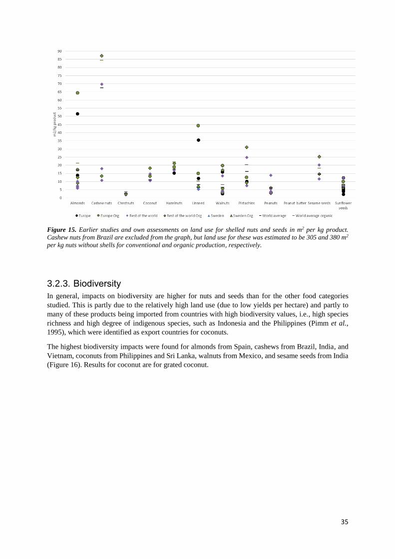
35

Figure 15. Earlier studies and own assessments on land use for shelled nuts and seeds in m2 per kg product.

Cashew nuts from Brazil are excluded from the graph, but land use for these was estimated to be 305 and 380 m2

per kg nuts without shells for conventional and organic production, respectively.

3.2.3. Biodiversity

In general, impacts on biodiversity are higher for nuts and seeds than for the other food categories

studied. This is partly due to the relatively high land use (due to low yields per hectare) and partly to

many of these products being imported from countries with high biodiversity values, i.e., high species

richness and high degree of indigenous species, such as Indonesia and the Philippines (Pimm et al.,

1995), which were identified as export countries for coconuts.

The highest biodiversity impacts were found for almonds from Spain, cashews from Brazil, India, and

Vietnam, coconuts from Philippines and Sri Lanka, walnuts from Mexico, and sesame seeds from India

(Figure 16). Results for coconut are for grated coconut.

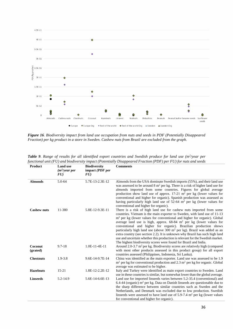
36

Figure 16. Biodiversity impact from land use occupation from nuts and seeds in PDF (Potentially Disappeared

Fraction) per kg product in a store in Sweden. Cashew nuts from Brazil are excluded from the graph.

Table 9. Range of results for all identified export countries and Swedish produce for land use (m2/year per

functional unit (FU) and biodiversity impact (Potentially Disappeared Fraction (PDF) per FU) for nuts and seeds

Product Land use

(m2/year per

FU)

Biodiversity

impact (PDF per

FU)

Comments

Almonds 5.0-64 5.7E-13-2.3E-12 Almonds from the USA dominate Swedish imports (55%), and their land use

was assessed to be around 8 m2 per kg. There is a risk of higher land use for

almonds imported from some countries. Figures for global average

production show land use of approx. 17-21 m2 per kg (lower values for

conventional and higher for organic). Spanish production was assessed as

having particularly high land use of 52-64 m2 per kg (lower values for

conventional and higher for organic).

Cashew nuts 11-380 5.8E-12-9.3E-11 There is a risk of high land use for cashew nuts imported from some

countries. Vietnam is the main exporter to Sweden, with land use of 11-13

m2 per kg (lower values for conventional and higher for organic). Global

average land use is high, approx. 68-84 m2 per kg (lower values for

conventional and higher for organic). Brazilian production shows

particularly high land use (above 300 m2 per kg). Brazil was added as an

extra country (see section 2.2). It is unknown why Brazil has such high land

use and uncertain whether this production is relevant for the Swedish market.

The highest biodiversity scores were found for Brazil and India.

Coconut

(grated)

9.7-18 1.0E-11-4E-11 Around 2.0-3.7 m2 per kg. Biodiversity scores are relatively high (compared

with most other products assessed in this product group) for all export

countries assessed (Philippines, Indonesia, Sri Lanka).

Chestnuts 1.9-3.8 9.6E-14-9.7E-14 China was identified as the main exporter. Land use was assessed to be 1.9

m2 per kg for conventional production and 2.3 m2 per kg for organic. Global

average was estimated to be higher.

Hazelnuts 15-21 1.8E-12-2.2E-12 Italy and Turkey were identified as main export countries to Sweden. Land

use in these countries is similar, but somewhat lower than the global average.

Linseeds 5.2-14.9 5.6E-14-6.6E-13 Land use for imported linseeds varies between 5.2-35.4 (conventional) and

6.4-44 (organic) m2 per kg. Data on Danish linseeds are questionable due to

the sharp difference between similar countries such as Sweden and the

Netherlands, and Denmark was excluded due to low production. Swedish

linseeds were assessed to have land use of 5.9-7.4 m2 per kg (lower values

for conventional and higher for organic).

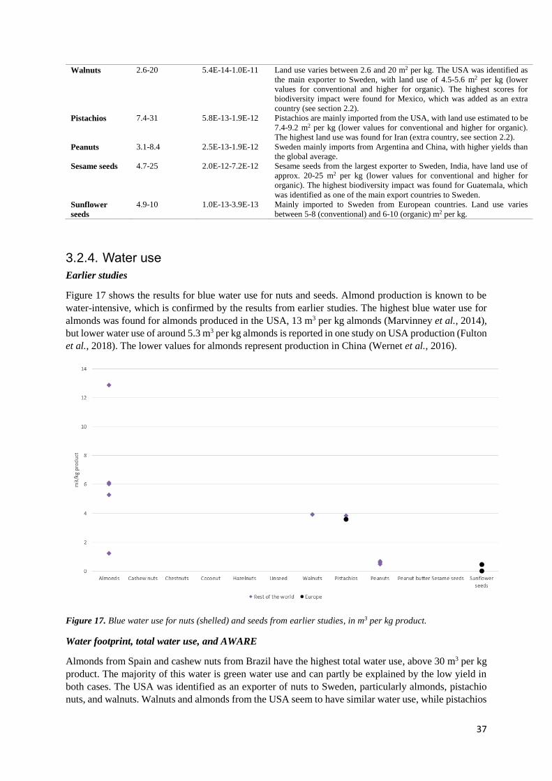
37

Walnuts 2.6-20 5.4E-14-1.0E-11 Land use varies between 2.6 and 20 m2 per kg. The USA was identified as

the main exporter to Sweden, with land use of 4.5-5.6 m2 per kg (lower

values for conventional and higher for organic). The highest scores for

biodiversity impact were found for Mexico, which was added as an extra

country (see section 2.2).

Pistachios 7.4-31 5.8E-13-1.9E-12 Pistachios are mainly imported from the USA, with land use estimated to be

7.4-9.2 m2 per kg (lower values for conventional and higher for organic).

The highest land use was found for Iran (extra country, see section 2.2).

Peanuts 3.1-8.4 2.5E-13-1.9E-12 Sweden mainly imports from Argentina and China, with higher yields than

the global average.

Sesame seeds 4.7-25 2.0E-12-7.2E-12 Sesame seeds from the largest exporter to Sweden, India, have land use of

approx. 20-25 m2 per kg (lower values for conventional and higher for

organic). The highest biodiversity impact was found for Guatemala, which

was identified as one of the main export countries to Sweden.

Sunflower

seeds

4.9-10 1.0E-13-3.9E-13 Mainly imported to Sweden from European countries. Land use varies

between 5-8 (conventional) and 6-10 (organic) m2 per kg.

3.2.4. Water use

Earlier studies

Figure 17 shows the results for blue water use for nuts and seeds. Almond production is known to be

water-intensive, which is confirmed by the results from earlier studies. The highest blue water use for

almonds was found for almonds produced in the USA, 13 m3 per kg almonds (Marvinney et al., 2014),

but lower water use of around 5.3 m3 per kg almonds is reported in one study on USA production (Fulton

et al., 2018). The lower values for almonds represent production in China (Wernet et al., 2016).

Figure 17. Blue water use for nuts (shelled) and seeds from earlier studies, in m3 per kg product.

Water footprint, total water use, and AWARE

Almonds from Spain and cashew nuts from Brazil have the highest total water use, above 30 m3 per kg

product. The majority of this water is green water use and can partly be explained by the low yield in

both cases. The USA was identified as an exporter of nuts to Sweden, particularly almonds, pistachio

nuts, and walnuts. Walnuts and almonds from the USA seem to have similar water use, while pistachios

38

from the USA have lower total water use. Grey water use for almonds and walnuts produced in the USA

is notably high, which indicates high nitrogen fertilizer application rates. Sesame seeds from India show

high green water use. Pistachios from Iran have high total water use (22 m3 per kg product), mostly blue

water (Mekonnen et al., 2011). Iran is the largest producer globally of pistachios, but is not among the

main exporters (FAOSTAT, 2019), indicating high domestic consumption.

Figure 18. Total water use, divided into green, blue, and grey water use, for nuts (shelled) and seeds, in m3 per

kg product in a store in Sweden, for the identified export countries, and world average water use for comparison.

0 5 10 15 20 25 30 35 40

Australia

Spain

USA

Chile (extra country)

Italy (extra european country)

World average

Vietnam

India (extra country)

Brazil (extra country)

World average

China

World average

Philippines

Indonesia (extra country)

Sri Lanka (extra country)

World average

Italy

Turkey

World average

Argentina

China

India

World average

USA

Ukraine (extra country)

Mexico (extra country)

Republic of Molodova (extra country)

World average

USA

Iran (extra country)

Turkey (extra country)

Greece (extra country)

World average

Denmark

Canada

The Netherlands

World average

Bulgaria

Romania

Russia

World average

India

Guatemala

Ethiopia

World average

Alm

on

dC

ash

ewC

hes

tnu

ts

Co

con

ut

Haz

eln

uts

Pea

nu

tW

alnu

tsP

ista

chio

sLi

nss

eed

sSu

nfl

ow

er s

eed

sSe

sam

e se

eds

m3/kg product

Green Blue Grey

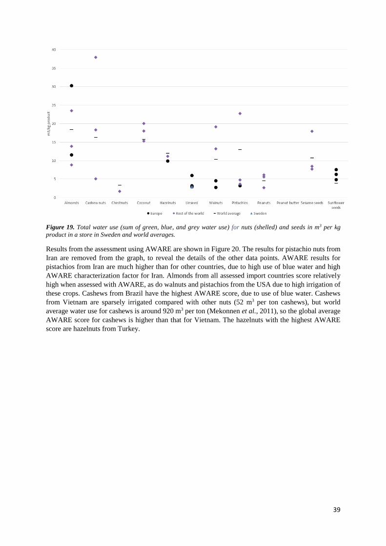
39

Figure 19. Total water use (sum of green, blue, and grey water use) for nuts (shelled) and seeds in m3 per kg

product in a store in Sweden and world averages.

Results from the assessment using AWARE are shown in Figure 20. The results for pistachio nuts from

Iran are removed from the graph, to reveal the details of the other data points. AWARE results for

pistachios from Iran are much higher than for other countries, due to high use of blue water and high

AWARE characterization factor for Iran. Almonds from all assessed import countries score relatively

high when assessed with AWARE, as do walnuts and pistachios from the USA due to high irrigation of

these crops. Cashews from Brazil have the highest AWARE score, due to use of blue water. Cashews

from Vietnam are sparsely irrigated compared with other nuts (52 m3 per ton cashews), but world

average water use for cashews is around 920 m3 per ton (Mekonnen et al., 2011), so the global average

AWARE score for cashews is higher than that for Vietnam. The hazelnuts with the highest AWARE

score are hazelnuts from Turkey.

40

Figure 20. Water use for nuts and seeds, assessed with the water scarcity method AWARE (Available Water

Remaining, m3eq per kg product) in a store in Sweden, and world averages. Pistachio nuts from Iran are excluded

from the graph, as their AWARE impact is above 1000 m3eq per kg product.

Table 10. Range of results for all identified export countries and Swedish produce for total water use (m3 per

functional unit (FU)) and AWARE (Available Water Remaining, m3eq per FU) for nuts (shelled) and seeds

Product Total water use

(m3 per FU)

AWARE (m3eq

per FU)

Commentsa

Almonds 9-30 78-330 Total water use differs greatly between export countries, global average is

intermediate. AWARE scores highest for Australia and Chile.

Cashew nuts 5-38 1-79 Total water use differs greatly between export countries, global average is

intermediate. AWARE score highest for India.

Chestnuts 2-3 3-9

Coconuts 15-20 0-21 Highest AWARE score found for global average production.

Hazelnuts 10-12 78-110 Total water use in main export countries to Sweden (Italy and Turkey) and

global average is similar.

Linseeds 3-6 0.3-14 Not irrigated in the three identified export countries (Denmark, Netherlands,

Canada), so AWARE scores are generally low. Highest AWARE score

found for global average production.

Walnuts 3-19 0-230 The largest exporter to Sweden, USA, was found to have an AWARE score

of 140 m3eq per kg product.

Pistachios 3-23 54-1130 The USA, the main export country to Sweden, has water use of 3.7 m3 per

kg product. Highest AWARE score found for Iran.

Peanuts 3-6 4-18 Total water use in the main export countries (Argentina, China, India) is

similar to the global average.

Sesame seeds 8-18 0-27 Water use in the main export country to Sweden (India) was estimated to be

higher than the global average water use for sesame seeds.

Sunflower

seeds

4-8 1-9

aComments included when applicable.

41

3.3. Carbohydrate sources

3.3.1. Climate impact

For barley, corn, millet, oats, rye, and wheat, the majority of the literature data show a climate impact

below 0.7 kg CO2e per kg edible product. A study on Australian corn (Maraseni et al., 2010) was

considered less relevant for the Swedish market. The identified export countries to the Swedish market

were France and Poland (SS, 2018), and South Africa was identified as the country with the largest trade

surplus of corn (FAOSTAT, 2019). Corn from South Africa has the second highest impact, around 0.7

kg CO2e per kg edible product, primarily due to the longer transport (0.4 kg CO2e per kg from transport).

Data for primary production of South African corn were taken from Agri-footprint (2018).

Two studies were found on quinoa, one scientific article (Cancino-Espinoza et al., 2018) and one

company report (Alter eco, 2012). The highest climate impact for quinoa was found for dark quinoa,

with around 0.9 kg CO2e per kg edible product (Alter eco, 2012). Rice has a higher climate impact than

the other cereals, but with large variation in the results. The higher climate impact is mainly due to the

methane emissions during wet rice cultivation. The large variation in results may be due to actual

variation in production methods and sites, combined with different methods to estimate methane

emissions (see e.g., Thanawong et al. (2014)). Data on European rice production were taken from two

studies (Kägi et al., 2010; Blengini & Busto, 2009).

All root vegetables have a climate impact below 0.5 kg CO2e per kg product, with the exception of

beetroot transported from Australia (Maraseni et al., 2010), sweet potato transported from Korea (So et

al., 2010), and frozen Jerusalem artichoke (lower value for fresh) (Landqvist & Woodhouse, 2015). The

study by Landqvist and Woodhouse (2015) on fresh and frozen Swedish products (carrots, swedes,

Jerusalem artichoke, parsnip) showed that processing and freezing doubles the climate impact of these

root vegetables. When comparing fresh and frozen products, it is important to note that the frozen

products have been cleaned, blanched, and frozen, which could potentially reduce energy use and waste

in the household. Further, root vegetables have a low climate impact in both cases (fresh and frozen)

compared with other products.

42

Figure 21. Climate impact of carbohydrate sources in kg CO2e per kg edible product in a store in Sweden. *Weight

of the product modified to equal 1 kg edible product, i.e., bread or ready-to-eat pasta or grains excluding the

emissions caused by energy use from baking and cooking. Note that the graph shows the climate impact from all

identified earlier studies for this product group, and not only those identified as relevant for the Swedish market.

Final assessments in Table 11 are based on relevance for the Swedish market.

Figure 22. Climate impact of fresh and frozen root vegetables, from Landqvist and Woodhouse (2015).

Table 11. Final assessment of climate impact of carbohydrate sources on the Swedish market Product Final assessment

(kg CO2e per kg

product in a

Swedish store)

No. of

relevant

references

Total no.

of

references

Comment

General Sweden

43

Cereals

Barley 0.5 0.5 9 (5 SW) 9 Most studies show an impact below 0.5 kg CO2e per

kg edible product. No clear difference between

Swedish and European barley.

Maize 0.5 4 6 European products considered most relevant for the

Swedish market.

Millet 0.3 1 1 Only one study was found, the recommendation is

therefore uncertain.

Oats 0.5 0.5 8 (4 SW) 8 All identified studies considered relevant for the

Swedish market.

Pasta 0.9 0.7 4 (2 SW) 4 All identified studies considered relevant for the

Swedish market.

Quinoa 0.9 No data 2 2 Two studies were identified, a scientific article

showing climate impact of Peruvian quinoa of 0.4 kg

CO2e per kg edible product (including transport to

Sweden) (2 references)

Rice 2.0 14 14 Climate impact in the studies varies between 0.5-2.0

kg CO2e per kg edible product. All data-points were

considered relevant for the Swedish market, indicating

that the climate impact of rice can vary greatly, but

some studies show that climate impact is likely to be

approximately 2 kg CO2e per kg edible product.

European rice may have a lower impact (below 1 kg

CO2e per kg edible product), but only two studies

investigated emissions from European rice

production.

Rye 0.5 0.5 5 (4 SW) 5 Earlier studies show that climate impact is likely to be

below 0.5 kg CO2e per kg edible product. No clear

difference was found between Swedish rye and

imported rye (from Europe).

Sorghum 0.5 1 1 Only one study was found, so this is an uncertain

assessment.

Wheat 0.6 0.6 12 (11

SW)

11 Studies on Swedish and European wheat production

considered relevant for the Swedish market. No clear

difference was found for Swedish and European

wheat.

Root vegetables

Beetroot 0.4 0.4 3 (2 SW) 4 European and Swedish production considered relevant

for the Swedish market.

Carrots 0.5 0.3 8 (6 SW) 10 European and Swedish production considered most

relevant for the Swedish market. Climate impact is

likely to be below 0.5 kg CO2e per kg product.

Swedish fresh products have lower impact with

transport added, fresh Swedish carrots have an impact

below 0.3 kg CO2e per kg product, European products

have a higher impact with transport added, between

0.2-0.5 kg CO2e per kg product.

Potatoes 0.4 0.3 9 (4 SW) 9 European and Swedish production considered relevant

for the Swedish market.

Swedes 0.5 0.5 2 (2 SW) 2 Swedish and European production considered relevant

for the Swedish market.

Sweet potato 0.8 No data 1 1 Only one study was found, the recommendation is

uncertain.

Jerusalem

artichoke

and parsnips

0.6 0.6 The results are based on one study (a report).

However, due to similarities with other production

(other root vegetables), climate impact is likely to be

below 0.6 kg CO2e per kg product.

3.3.2. Land use

Land use for Swedish production and Swedish imports of carbohydrate sources and root vegetables is

presented in Figure 23. The results show that millet requires more land than other cereals, due to lower

yields. Global average land use for millet, quinoa, and sorghum is clearly higher than for Swedish

imports, due to higher yields in countries found to export to Sweden. The higher values for the global

44

average production can be seen as an indicator that these products may be associated with higher land

use than the current Swedish imports show.

Root vegetables all have low land use, below 1 m2 per kg product. For root vegetables, organic

production was assumed to have slightly higher yields (5%) than conventional. This was based on three

earlier studies on sweet potato and sugar beet (De Ponti et al., 2012). In this study, 5% higher yield for

organic was assumed for beetroot, carrots, sweet potato, parsnip, and Jerusalem artichoke. We found no

statistics on yields of organic and conventional carrot production, or any other root vegetables. Official

yield statistics for root vegetables in Sweden include both organic and conventional production, but do

not show them separately.

For potatoes, organic potato yield in De Ponti et al. (2012) was 70% of the conventional yield. For

Swedish organic potato production, yield was 50%-68% of the conventional yield in 2013-2018, with

higher yield toward the end of this period (SBA, 2019).

When comparing root vegetables with cereals in Figure 23, it is important to note that although the

cereals were recalculated to edible products, they generally have a lower water content and a higher

energy content than the raw root vegetables (which were assumed to be edible as-is, or to undergo very

little change during cooking to edible form).

Land use for Swedish quinoa production was estimated to be 2.3-2.9 m2 per kg (lower values for

conventional and higher for organic), based on yield data from Hushållningssällskapet (2013).

Figure 23. Land use for carbohydrate sources in m2 per kg product in a store in Sweden and world averages.

*Weight of the product modified to equal 1 kg edible product, i.e., bread or ready-to-eat pasta or grains. Energy

use for cooking was not included.

3.3.3. Biodiversity

Impact on biodiversity from land use was generally below 2E-13 PDF per kg product for carbohydrate

sources (Figure 24). This is primarily due to the relatively low land use, but also to the fact that most of

these products are either produced in Sweden or imported from northern European countries with quite

low biodiversity in natural vegetation. Millet from India and quinoa from Peru and Bolivia are clear

45

exceptions, with (for this group) much higher impact than the other products due to low yields and high

biodiversity in these regions.

Figure 24. Biodiversity impact from land use occupation from carbohydrate sources in PDF (Potentially

Disappeared Fraction) per kg edible product in a store in Sweden. *Weight of the product modified to equal 1 kg

edible product, i.e., bread or ready-to-eat pasta or grains.

Table 12. Range of results for all identified export countries and Swedish produce for land use (m2/year per

functional unit (FU)) and biodiversity impact (Potentially Disappeared Fraction (PDF) per FU) for carbohydrate

sources Product Land use

(m2/year per

FU)

Biodiversity

impact (PDF per

FU)

Commenta

Cereals

Barley 0.9-3.0 1.2E-14-6.1E-14 The higher values are for conventional and organic production based on the

global average, indicating a risk of somewhat higher land use if imports

come from other countries than those included in this report. Swedish

produce has land use of 1.3 m2 per kg for conventional and 1.9 m2 per kg

product for organic.

Corn 0.6-1.2 1.8E-14-2.8E-13

Millet 3.2-6.4 6.7E-14-1.1E-12 Biodiversity impact highest for India.

Oats 1.2-2.1 1.4E-14-2.2E-14

Pasta 0.9-3.9 1.1E-14-4.2E-13 Swedish pasta has land use of 1.1-1.6 m2 per kg (lower values for

conventional and higher for organic). The highest land use is in Turkey,

which was not identified as a main exporter to Sweden, but is the main

exporter globally of wheat. The highest biodiversity impact was found for

Italy and Turkey.

Quinoa 1.5-5.0 1.1E-12-1.6E-12 Bolivia has the highest land use and the highest biodiversity impact. Sweden

has very limited quinoa production, and land use was estimated to be 2.3-2.9

m2 per kg (lower values for conventional and higher for organic).

Rice 0.6-1.0 1.3E-13-2.3E-13 Land use in the main export countries identified (India, Italy, Thailand) is

similar to the global average.

46

Rye 1.0-2.8 1.6E-14-5.1E-14 Global average similar to that in the main export countries. Land use for

Swedish production is approximately 1.0-1.3 m2 per kg (lower values for

conventional and higher for organic).

Sorghum 1.1-4.0 8.6E-14-1.1E-13 Main export country (USA) has lower land use than the global average.

Wheat 0.8-3.3 9.1E-15-3.5E-13 Land use for Swedish import varies between 0.8-2.4 (conventional) and 1.0-

3.3 (organic) m2 per kg. Highest land use and biodiversity impact were found

for Turkey. Land use for Swedish production is approx. 1.0-1.3 m2 per kg

(lower values for conventional and higher for organic).

Root vegetables

Beetroot 0.4 3.2E-15-7.6E-15 Only data on Swedish production. Land use in other countries was assumed

to be the same as for Swedish production, likely 0.4 m2 per kg.

Carrots 0.2-0.3 2.0E-15-4.2E-14 Similar land use for Swedish and imported products.

Potatoes 0.3-0.7 3.5E-15-1.4E-14 Land use is likely to be 0.3-0.7 m2 per kg. Swedish potatoes were assessed

to have land use of 0.4 m2 per kg.

Sweet potato 0.4-0.8 3.3E-14-3.4E-14

Parsnip,

swedes and

Jerusalem

artichoke

0.5-1.0 3.7E-15-6.7E-15 Only data on Swedish production found. Land use is likely to be around 0.5

m2 per kg for Swedes and parsnips, and around 1 m2 per kg for Jerusalem

artichoke.

aComments included when applicable.

3.3.4. Water use

Earlier studies

Water use is rarely included in earlier studies on the climate impact of carbohydrate sources (Figure 25).

One study on rice shows high blue water use, of around 1.6 m3 per kg rice (Blengini & Busto, 2009).

Blue water use in carrot production is included in the ecoinvent database (Wernet et al., 2016) and the

study by Fuentes et al. (2006). Blue water use in carrot production from these data sources varies

between 0.03-0.12 m3 per kg carrots.

Figure 25. Blue water use from earlier studies on carbohydrate sources. *Weight of the product modified to equal

1 kg edible product, i.e., bread or ready-to-eat pasta or grains.

47

Water footprint, total water use, and AWARE

Looking at water use in Mekonnen et al. (2011), divided into green, blue, and grey water (Figure 26)

and as total water (Figure 27), total water use is highest for quinoa and millet, most likely due to lower

yields. Blue water use is highest for rice, indicating high irrigation rates in all three identified export

countries (India, Thailand, Italy) but also for the world average production.

48

Figure 26. Total water use, divided into green, blue, and grey water use, for carbohydrate sources in m3 per kg

edible product in a store in Sweden for the identified export countries, and world average water use for

comparison.

0 1 2 3 4 5 6 7

Denmark

Finland

UK

France

World average

Sweden

France

Poland

South Africa

Brazil (extra country)

Argentina (extra country)

World average

India

Ukraine

World average

Denmark

Finland

Canada

World average

Sweden

Peru

Bolivia

World average

India

Italy

Thailand

World average

Denmark

Finland

Poland

Germany

World average

Sweden

USA

World average

Denmark

Finland

Germany

Turkey

World average

Sweden

The Netherlands

Denmark

Germany

World average

Sweden

Italy

The Netherlands

China

World average

Sweden

Denmark

Finland

France

World average

Sweden

USA

World average

Bar

ley

Mai

zeM

illet

Oat

sQ

uin

oa

Ric

eR

yeSo

rgh

um

Wh

eat

Bee

tro

ot

Car

rot

Po

tato

esSw

eet

po

tato

es

m3/kg product

Green Blue Grey

49

Figure 27. Total water use (sum of green, blue, and grey water use) for carbohydrate sources in m3 per kg edible

product in a store in Sweden, and for the world average. *Weight of the product modified to equal 1 kg edible

product, i.e., bread or ready-to-eat pasta or grains.

When applying the water scarcity indicator AWARE, rice from Italy has a higher impact due to large

amounts of blue water and high AWARE characterization factors for Italy (Figure 28). Further, global

average production of rice and wheat uses relatively large amounts of blue water (Mekonnen et al.,

2011) which is the reason behind the higher impacts. In general, both total water use and AWARE

indicators are low compared with e.g., those for some nuts.

50

Figure 28. Water use for carbohydrate sources assessed with the water scarcity method AWARE (Available Water

Remaining) in m3eq per kg product in a store in Sweden and the world average. *Weight of the product modified

to equal 1 kg edible product, i.e., bread or ready-to-eat pasta or grains.

Table 13. Range of results for all identified export countries and Swedish produce for total water use (m3 per

functional unit (FU)) and AWARE (Available Water Remaining, m3eq per FU) for carbohydrate sources

Product Total water

use (m3 per

FU)

AWARE (m3eq

per FU)

Comment

Barley 0.3-0.9 0-2.3 Total water use for Swedish production and Swedish imports is likely

to be below 0.4 m3 per kg. Global average is 0.9 m3 per kg. For

Sweden and the main import countries, the AWARE score is 0 m3eq

(or close to), due to no or very low irrigation rates. The AWARE

value is higher for world average production.

Corn 0.4-1.2 0-2.4 Assessed to be below 0.8 m3 per kg for the identified European

export countries (France and Poland), global average water use is

also below 0.8 m3 per kg. South Africa and Brazil have total water

use of 1.2 m3 per kg. South Africa was identified as the main exporter

globally and Brazil was added as an extra country in the analysis.

Millet 1.5-2.3 0-1.3

Oats 0.5-1.5 0-7.0 Water use in the main export countries (Finland and Denmark) and

in Sweden is likely to be below 0.6 m3 per kg. Global average and

the largest global exporter (Canada) have higher water use, around

1.0-1.5 m3 per kg. A higher AWARE score was found for global

average production.

Pasta 0.5-1.9 0-12 Italian pasta was assessed to have total water use of around 1 m3 per

kg. Pasta made of wheat from Turkey (identified as main exporter of

wheat) or global average wheat was estimated to have the highest

total water use. Highest AWARE score found for global average

production.

Quinoa 1.2-2.0 0.13-0.76

51

Rice 0.6-1.3 1.6-12 Water use varied between 0.6 (Italy) and 1.3 m3 per kg. Proportion

of blue water in total water is relatively high in all identified export

countries and in the global average.

Rye 0.3-1.3 0-0.9 Water use in Sweden, Denmark, and Germany is below or close to

0.6 m3 per kg. Global average, Finland, and Poland have slightly

higher water use, of around 1.1-1.3 m3 per kg. For Sweden and the

main import countries, the AWARE score is 0 m3eq (or close to) due

to no or very low irrigation rates. A higher AWARE value was found

for world average production.

Wheat 0.4-1.6 0-10 Most Swedish imports and Swedish production have water use below

0.5 m3 per kg. Turkey was identified as the largest exporter globally

and is the country with the highest water use (of the countries

assessed) with approx. 1.5 m3 per kg. A higher AWARE value was

found for world average production.

Root vegetables

Beetroot No data.

Carrots 0.04-0.4 0-2.2 All export countries assessed, Swedish production, and global

average show water use below 0.4 m3 per kg. Highest AWARE score

found for Italian production. Italy was identified as the main exporter

of carrots to Sweden.

Potatoes 0.15-0.4 0.1-2.3 All export countries assessed, Swedish production, and global

average have water use below 0.4 m3 per kg. A higher AWARE value

was found for world average production.

Swedes No data.

Sweet

potatoes

0.5-1.2 0.3-2.9 The largest exporter to Sweden (USA) has water use of 1.2 m3 per

kg. Global average water use is around 0.5 m3 per kg. A higher

AWARE score was found for the USA.

3.4. Plant-based drinks and cream

3.4.1. Climate impact

Results from earlier studies on plant-based drinks and cream are shown in Figure 29. As earlier studies

used functional units based on volume (e.g., 1 liter) and based on mass (e.g., 1 kg), it was assumed that

1 liter plant-based drink equals 1 kg (the functional unit used in the Vego-guide). In general, all drinks

and plant-based cream alternatives have a climate impact below 1 kg CO2e per kg product. Swedish oat

drink has the lowest impact, around 0.24-0.34 kg CO2e per kg (Florén et al., 2013), mainly explained

by the shorter transport.

For plant-based cream alternatives, climate impact for oat cream is just above 0.5 kg CO2e per kg

(Nilsson & Florén, 2015). No data on coconut cream and soy-based cream could be found, so the value

in Table 14 is based on calculations made in this report (see Appendix A3) and climate impact values

from the ecoinvent database (Wernet et al., 2016). Following the methodology applied in this report,

transport from North America was added for almond, coconut, and soy drink, since the studies originated

from the USA or Canada. This means that the data in Figure 29 for many products show the impact of

transporting mainly water long distances (the drinks typically contain 90-92% water). The climate

impact will hence be considerably lower if the drinks are produced in Sweden or closer to Sweden, i.e.,

only the raw materials are transported long distances. This is probably the case for products on the

Swedish market, particularly when the market for plant-based drinks and cream increases. For

comparison, Figure 29 also shows the climate impact from Swedish dairy milk and cream (Moberg et

al., 2019; Röös, 2012).

52

Figure 29. Climate impact of plant-based drinks and cream in kg CO2e per kg product in a store in Sweden. Note

that the graph shows the climate impact from all identified earlier studies for this product group, and not only

those identified as relevant for the Swedish market. Recommendations in Table 14 are based on relevance for the

Swedish market.

Table 14. Final assessment of the climate impact of plant-based drinks and cream on the Swedish market

Product Final assessment

(kg CO2e per kg

product in a

Swedish store)

No. of

relevant

references

Total no.

of

references

Comment

General Sweden

Almond

drink

0.8

4 4 Likely to have climate impact below 0.8 kg CO2e per

liter.

Coconut

drink

0.4 1 1 Only one reference was found, assessment uncertain.

Soy drink 0.7 5 5 Climate impact is likely well below 0.7 kg CO2e per

kg, due to lower impact from shorter transport than

assessed in the studies identified. The shorter transport

is because the product is likely to be produced in

Europe, for the European market.

Oat drink 0.3 0.3 1 1 Only one study was found, showing that oat drink

produced in Sweden has a climate impact below 0.34

kg CO2e per kg. However, that study was assessed to

be of high quality and very relevant for the Swedish

market.

Oat cream 0.5 0.5 1 1 Only one study was found, showing that oat cream

produced in Sweden has a climate impact below 0.52

kg CO2e per kg. However, that study was assessed to

be of high quality and very relevant for the Swedish

market.

Coconut

milk

1.2 Own

assess-

ment

Climate impact was estimated based on climate impact

of coconuts and yield of coconut milk (see Appendix

A3). Impacts from land use change were excluded in

the final assessment.

53

3.4.2. Land use

Combined assessment of land use (earlier studies plus own assessment)

Land use and biodiversity impacts for plant-based drinks and cream (Figure 30) were estimated based

on the raw material ingredients (Appendix A3) and data from earlier studies. Coconut milk (fat content

17%) was found to have the highest land use. However, the amount of coconut needed to produce 1 kg

of coconut milk was not known and was estimated based on mass balance (see Appendix A3 and Kool

et al. (2012)). The results are therefore uncertain. Results from earlier studies (Nilsson & Florén, 2015)

on oat cream show relatively high land use compared with that based on the ingredients (Appendix A3).

Rapeseed was found to be most land-demanding for oat cream. Nilsson and Florén (2015) used

economic allocation to allocate between rapeseed oil and rapeseed cake, while in this report mass

allocation was used, which could explain the difference in the results.

Figure 30. Land use for plant-based drinks and cream, and dairy milk and cream, in m2 per kg in a store in

Sweden, and the global average.

3.4.3. Biodiversity

Coconut milk has the highest impact as regards biodiversity loss, due to high biodiversity in the areas

in which coconuts are produced. All other products have a relatively low impact, again because they do

not contain as much raw material (mainly water).

Several products that are substitutes for hard cheese contain coconut oil. The largest exporter of coconuts

to Sweden is the Philippines and the largest producer globally is Indonesia. Both are tropical countries

with relatively high biodiversity impact factors from land use (Chaudhary et al., 2018), and therefore

there is a risk that these products are associated with high impact on biodiversity. However, the impact

from these products was not included in the assessment.

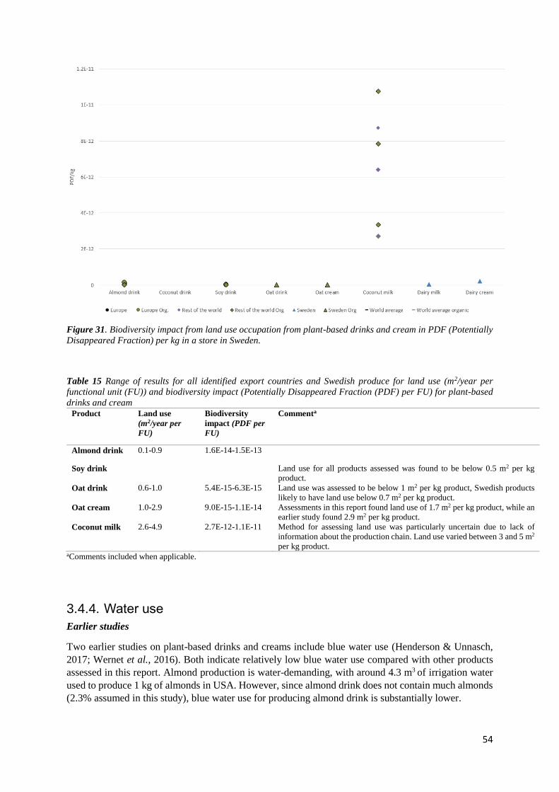
54

Figure 31. Biodiversity impact from land use occupation from plant-based drinks and cream in PDF (Potentially

Disappeared Fraction) per kg in a store in Sweden.

Table 15 Range of results for all identified export countries and Swedish produce for land use (m2/year per

functional unit (FU)) and biodiversity impact (Potentially Disappeared Fraction (PDF) per FU) for plant-based

drinks and cream Product Land use

(m2/year per

FU)

Biodiversity

impact (PDF per

FU)

Commenta

Almond drink 0.1-0.9 1.6E-14-1.5E-13

Soy drink Land use for all products assessed was found to be below 0.5 m2 per kg

product.

Oat drink 0.6-1.0 5.4E-15-6.3E-15 Land use was assessed to be below 1 m2 per kg product, Swedish products

likely to have land use below 0.7 m2 per kg product.

Oat cream 1.0-2.9 9.0E-15-1.1E-14 Assessments in this report found land use of 1.7 m2 per kg product, while an

earlier study found 2.9 m2 per kg product.

Coconut milk 2.6-4.9 2.7E-12-1.1E-11 Method for assessing land use was particularly uncertain due to lack of

information about the production chain. Land use varied between 3 and 5 m2

per kg product. aComments included when applicable.

3.4.4. Water use

Earlier studies

Two earlier studies on plant-based drinks and creams include blue water use (Henderson & Unnasch,

2017; Wernet et al., 2016). Both indicate relatively low blue water use compared with other products

assessed in this report. Almond production is water-demanding, with around 4.3 m3 of irrigation water

used to produce 1 kg of almonds in USA. However, since almond drink does not contain much almonds

(2.3% assumed in this study), blue water use for producing almond drink is substantially lower.

55

Figure 32. Blue water use for plant-based dairy, in m3 per kg in a store in Sweden.

Water footprint, total water use, and AWARE

Based on the ingredients and the process requirements (Appendix A3), total water use and water use

using AWARE were calculated. Note that process water requirements were only found (and included)

for soy and oat drinks and oat cream, and not for the other products. However, process water use is small

in relation to the amount of water used by the crops. Results for total water use are shown in Figures 33

and 34 and AWARE scores in Figure 35.

Global average production of oat drink, oat cream, and coconut drink is based on crops which are

irrigated to a larger extent than Swedish oat drink and oat cream or coconut drink from the Philippines,

Sri Lanka, and Indonesia (Mekonnen et al., 2011). This, combined with a higher AWARE score for the

global average than for Sweden and the Philippines (Boulay et al., 2018), contributed to global average

production having much higher AWARE scores than Swedish and Philippian production (Figure 33).

This is especially important in the case of coconut drink, since import statistics on coconut products do

not specify coconut drink, and therefore coconut imports were used to find likely export country for

coconut drink. This assumption is uncertain, and global average production therefore provides valuable

additional information. For oat products, however, the raw material is likely produced in Sweden.

56

Figure 33. Total water use, divided into green, blue, and grey water use, for plant-based drinks and cream, and

dairy milk and cream, in m3 per kg product in a store in Sweden, and world averages.

Figure 34. Total water use (sum of green, blue, and grey water use) for plant-based dairy and cream, and dairy

milk and cream, assessed in m3 per kg product in a store in Sweden, and world averages.

0 1 2 3 4 5 6 7

USA

Australia

Spain

World average

Italy

USA

World average

Sweden

World average

Sweden

World average

Philippines

Indonesia (extra country)

Sri Lanka (extra country)

World average

Sweden

World average

Sweden

World average

Alm

on

d d

rin

kSo

y d

rin

kO

at m

ilkO

at c

ream

Co

con

ut

crea

mM

ilkC

ream

m3/kgGreen Blue Grey

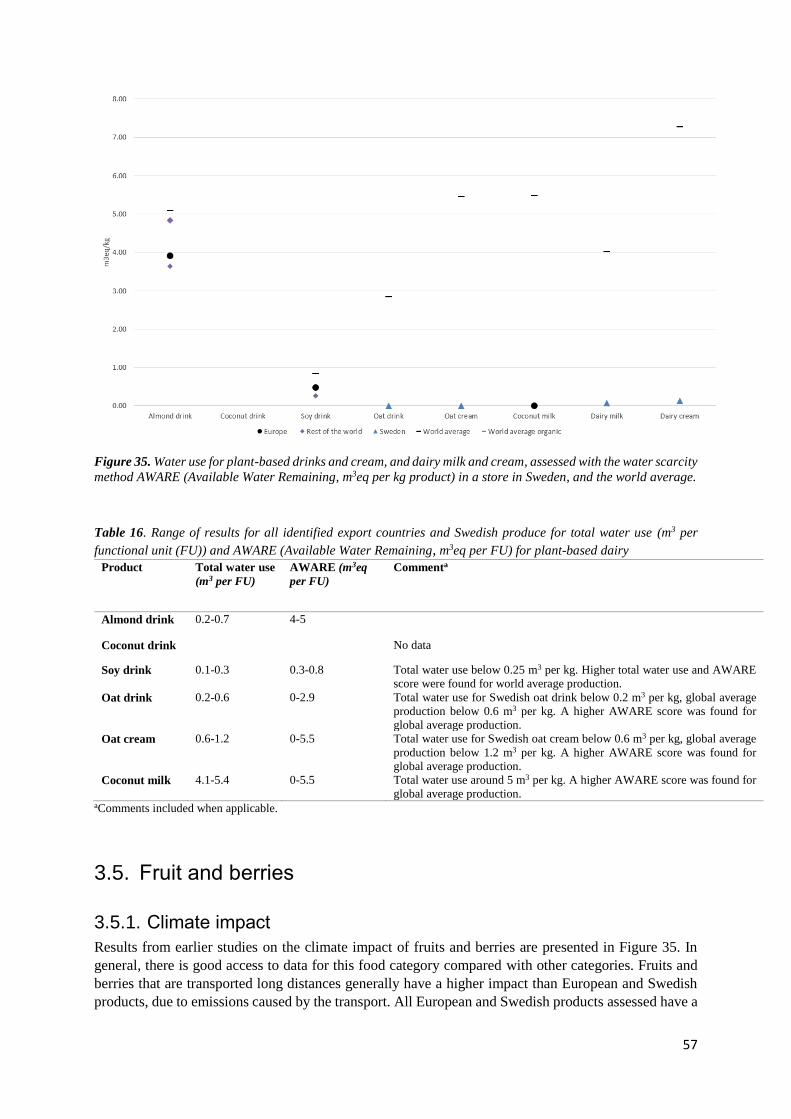
57

Figure 35. Water use for plant-based drinks and cream, and dairy milk and cream, assessed with the water scarcity

method AWARE (Available Water Remaining, m3eq per kg product) in a store in Sweden, and the world average.

Table 16. Range of results for all identified export countries and Swedish produce for total water use (m3 per

functional unit (FU)) and AWARE (Available Water Remaining, m3eq per FU) for plant-based dairy

Product Total water use

(m3 per FU)

AWARE (m3eq

per FU)

Commenta

Almond drink 0.2-0.7 4-5

Coconut drink No data

Soy drink 0.1-0.3 0.3-0.8 Total water use below 0.25 m3 per kg. Higher total water use and AWARE

score were found for world average production.

Oat drink 0.2-0.6 0-2.9 Total water use for Swedish oat drink below 0.2 m3 per kg, global average

production below 0.6 m3 per kg. A higher AWARE score was found for

global average production.

Oat cream 0.6-1.2 0-5.5 Total water use for Swedish oat cream below 0.6 m3 per kg, global average

production below 1.2 m3 per kg. A higher AWARE score was found for

global average production.

Coconut milk 4.1-5.4 0-5.5 Total water use around 5 m3 per kg. A higher AWARE score was found for

global average production. aComments included when applicable.

3.5. Fruit and berries

3.5.1. Climate impact

Results from earlier studies on the climate impact of fruits and berries are presented in Figure 35. In

general, there is good access to data for this food category compared with other categories. Fruits and

berries that are transported long distances generally have a higher impact than European and Swedish

products, due to emissions caused by the transport. All European and Swedish products assessed have a

58

climate impact below 1 kg CO2e per kg product in a Swedish store, with the exception of melons from

unheated greenhouses (Cellura et al., 2012) and watermelon and raspberries/blueberries from Europe

(country unspecified) (Audsley et al., 2010).

In general, emissions from transport are more important for fruits and berries, which generally have a

low climate impact per kg product from primary production. This is one of the reasons why some studies

on products from “rest of the world” report climate impact higher than 1 kg CO2e per kg in a Swedish

store. World average production of dates and organic and non-organic (fresh) dates (Wernet et al., 2016)

show the highest climate impact, above 4 kg CO2e per kg product (including transport). This is primarily

due to high emissions of nitrous oxide (N2O) from fertilizer use.

Some products in this product group are transported to Sweden by air, which causes exceptionally high

emissions from transport. Airfreighted products include some berries produced outside Europe and some

exotic fruits with short durability, such as starfruit. Common exotic fruits such as bananas, pineapple,

and the most common mango type sold in Swedish stores have longer duration times and are generally

transported by boat, with a lower climate impact (per kg product transported) (SverigesKonsumenter,

2018). The data in Figure 35 only include one study that considered air transport, for pineapple (Brenton

et al., 2010), and it was considered less relevant for the Swedish market. For more information on how

climate impact from air transport was estimated, see section 2.3.

Strawberries for the Swedish market are primarily sourced from within Europe. According to import

statistics, around 40% of strawberry imports to Sweden come from Belgium (SS, 2018). Belgium

strawberry production can be in heated or unheated greenhouses (Proefcentrum, 2019). No earlier study

was found on Belgian strawberries, and the climate impact and energy use is therefore unknown. Further,

no data were found on wild blueberries or lingonberries. For raspberries, one study (Foster et al., 2014)

showed much higher impact than the other studies, but was only presented in a conference abstract and

provided little information about reasons for the relatively high impact compared with other studies on

raspberries and other berries.

Figure 36. Climate impact of fruits and berries in kg CO2e per kg product in a store in Sweden. Note that the

graph shows the climate impact from all identified earlier studies for this product group, and not only those

identified as relevant for the Swedish market. Final assessments in Table 17 are based on relevance for the Swedish

market.

59

Table 17. Final assessment of the climate impact of fruits and berries on the Swedish market Product Final assessment

(kg CO2e per kg

product in a

Swedish store)

No. of

relevant

references

Total no.

of

references

Comment

General Sweden

Apples 0.5 0.2 14 (2 SW) 24 European apple production considered relevant for the

final assessment. Only one study on European apple

production shows an impact slightly above 1 kg CO2e

per kg product, for an old low-yielding orchard not

representative of all orchards. Apples from outside

Europe are likely to have a climate impact below 1 kg

CO2e per kg product.

Apricots 0.7 3 3 European apricot production was considered for the

general final assessment. There was no difference

between European production and production outside

Europe.

Bananas 1.5 13 13 All studies were considered relevant for the general

recommendation. Many studies show an impact below

1 kg CO2e per kg.

Cherries 0.8 4 4 All studies considered relevant in the general

recommendation. European cherries likely to have an

impact below 0.5 kg CO2e per kg. Possibly sometimes

transported by air, no earlier study was found on air

transport of cherries.

Dates 4 2 2 All studies considered relevant for the

recommendation.

Figs 0.6 1 1 Only one study was found, the assessment is

uncertain.

Grapefruits

and pomelo

0.8 1 1 Only one study was found, the assessment is

uncertain.

Grapes 1.3 11 11 All studies considered relevant for the final

assessment. European grapes are likely to have a

climate impact below 0.7 kg CO2e per kg grapes (8

references).

Guavas and

mango

1.9 4 4 All studies considered relevant for the final

assessment. Possibly sometimes transported by air, no

earlier study was found on air transport of guavas and

mango.

Kiwifruit 1 9 9 All studies considered relevant for the final

assessment. European production tends to have

slightly lower impact, but no clear trend.

Lemons and

limes

0.8 5 5 All studies considered relevant for the final

assessment. No clear difference between European

products and “rest of the world”.

Melons 1.9 9 9 All studies considered relevant for the final

assessment. No clear trend between European

products and “rest of the world”. Melons are

sometimes produced in greenhouses, which can

explain the large variation in results.

Oranges 0.7 9 9

All studies considered relevant for the final

assessment. No clear difference between European

products and “rest of the world” was found.

Papayas 1 1 1 Only one study was found, the assessment is

uncertain. High risk of air transport, no study that

considered air transport for papaya was found.

Peaches 0.5 4 8

European production was considered for the final

assessment. Production outside Europe is likely to

have an impact below 1.2 kg CO2e per kg peaches.

Pears 0.8 0.2 7 (1 SW) 9 Only European production was considered for the

final assessment. “Rest of the world” production is

likely to have a climate impact below 1 kg CO2e per

kg pears. Data on Swedish production are only based

on one study, the assessment is uncertain.

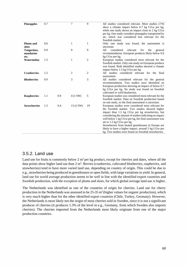
60

Pineapples 0.7 7 9 All studies considered relevant. Most studies (7/9)

show a climate impact below 0.7 kg CO2e per kg,

while one study shows an impact close to 2 kg CO2e

per kg. One study considers pineapples transported by

air, which was considered less relevant for the

Swedish market.

Plums and

sloes

0.6 1 1 Only one study was found, the assessment is

uncertain.

Tangerines,

mandarins

etc.

0.9 9 9 All considered relevant for the general

recommendation. European products likely below 0.6

kg CO2e per kg.

Watermelon 1.5 1 2 European studies considered most relevant for the

Swedish market. Only one study on European produce

was found. Both identified studies showed a climate

impact below 1.5 kg CO2e per kg.

Cranberries 1.5 2 2 All studies considered relevant for the final

assessment.

Blueberries 0.9 3 3 All studies considered relevant for the general

recommendation. Two studies were identified on

European production showing an impact of below 0.7

kg CO2e per kg. No study was found on Swedish

cultivated or wild blueberries.

Raspberries 1.1 0.9 4 (1 SW) 5 European studies was considered most relevant for the

Swedish market. Data on Swedish production based

on one study, so the final assessment is uncertain.

Strawberries 1.5 0.4 13 (2 SW) 19 European studies were considered most relevant for

the Swedish market. Two studies showed higher

impact than 1.5 kg CO2e per kg strawberries, but

considering the amount of studies indicating an impact

well below 1 kg CO2e per kg, the final assessment was

set to 1.5 kg CO2e per kg.

Strawberries from heated greenhouses in Europe are

likely to have a higher impact, around 3 kg CO2e per

kg. Two studies were found on Swedish strawberries.

3.5.2. Land use

Land use for fruits is commonly below 2 m2 per kg product, except for cherries and dates, where all the

data points show higher land use than 2 m2. Berries (cranberries, cultivated blueberries, raspberries, and

strawberries) tend to have more varied land use, depending on country of origin. This could be due to

e.g., strawberries being produced in greenhouses or open fields, with large variations in yield. In general,

land use for world average production seems to be well in line with the identified export countries and

Swedish production, with the exception of plums and sloes, for which global average land use is higher.

The Netherlands was identified as one of the countries of origin for cherries. Land use for cherry

production in the Netherlands was assessed to be 25-35 m2 (higher values for organic production), which

is very much higher than for the other identified export countries (Chile, Turkey, Germany). However,

the Netherlands is most likely not the origin of most cherries sold in Sweden, since it is not a significant

producer of cherries (it produces 1.3% of the level in e.g., Germany, from which Sweden also imports

cherries). The cherries imported from the Netherlands most likely originate from one of the major

production countries.

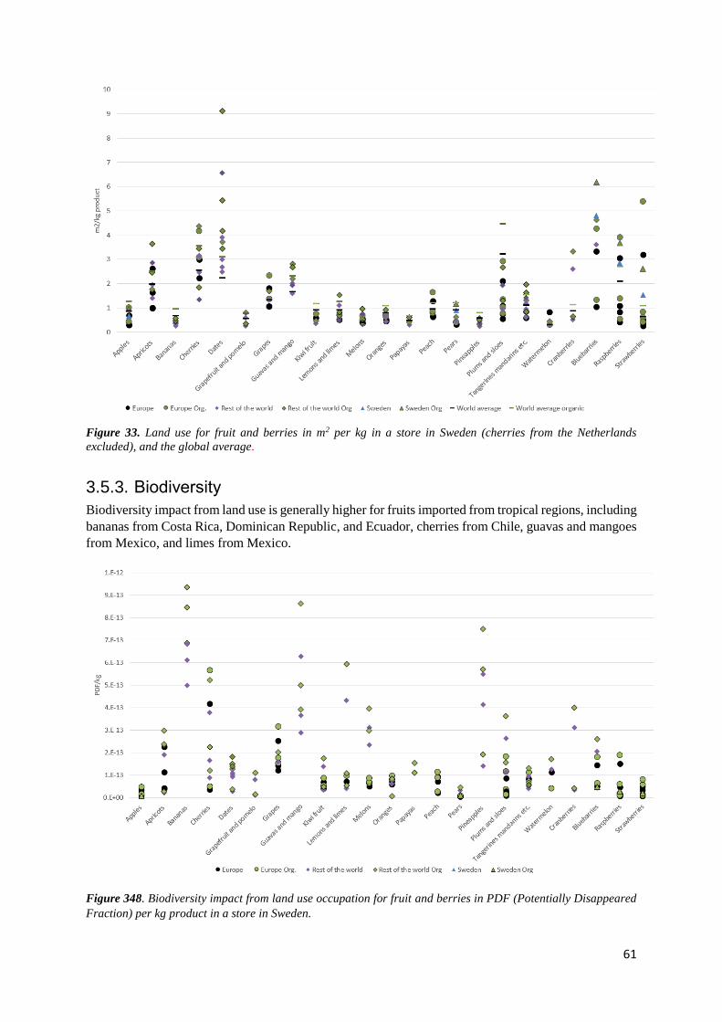
61

Figure 33. Land use for fruit and berries in m2 per kg in a store in Sweden (cherries from the Netherlands

excluded), and the global average.

3.5.3. Biodiversity

Biodiversity impact from land use is generally higher for fruits imported from tropical regions, including

bananas from Costa Rica, Dominican Republic, and Ecuador, cherries from Chile, guavas and mangoes

from Mexico, and limes from Mexico.

Figure 348. Biodiversity impact from land use occupation for fruit and berries in PDF (Potentially Disappeared

Fraction) per kg product in a store in Sweden.

62

Table 18. Range of results for all identified export countries and Swedish produce for land use (m2/year per

functional unit (FU)) and biodiversity impact (Potentially Disappeared Fraction) (PDF) per FU) for fruits and

berries

Product Land use

(m2/year per

FU)

Biodiversity

impact (PDF per

FU)

Commenta

Fruit

Apples 0.3-1.0 5.2E-15-4.7E-14

Apricots 1.0-3.6 2.1E-14-3.0E-13 Turkey, which was added as an extra country (see section 2.2), has the

highest land use of the countries assessed. The highest biodiversity impact

was found for Armenia and Turkey. Spain was identified as the largest

exporter globally.

Bananas 0.3-1.0 5.0E-13-8.4E-13 Land use varies between 0.3-0.7 (conventional) and 0.4-1.0 (organic) m2 per

kg.

Cherries 1.3-4.4 3.6E-14-5.7E-13 Products from the Netherlands excluded from the analysis. The highest

biodiversity impact was found for Chile (largest exporter globally) and Spain

(extra country, see section 2.2)

Dates 2.2-9.1 2.7E-14-1.8E-13

Grapefruits

and pomelo

0.2-0.8 1.0E-14-1.1E-13

Grapes 1.1-2.3 1.2E-13-3.2E-13 The highest biodiversity impact was found for Spain.

Guavas and

mango

1.6-2.7 2.9E-13-8.6E-13 The highest biodiversity impact was found for Mexican production, Mexico

was identified as the main exporter globally.

Kiwifruit 0.4-1.2 6.8E-14-1.7E-13

Lemons and

lime

0.5-1.5 3.5E-14-5.9E-13 The highest biodiversity impact was found for Mexican production, Mexico

was identified as the main exporter globally.

Melons 0.3-1.0 5.1E-14-3.9E-13 The highest biodiversity impact was found for Guatemala production,

Guatemala was identified as the main exporter globally.

Oranges 0.4-1.1 3.9E-15-9.7E-14

Papayas 0.3-0.7 8.1E-14-1.5E-13

Peach 0.6-1.6 2.1E-14-1.1E-13

Pears 0.3-1.2 5.4E-15-4.4E-14

Pineapples 0.2-0.8 1.4E-13-5.7E-13

Plums and

sloes

0.6-4.5 9.6E-15-3.6E-13 Global average had the highest land use. South Africa, added as an extra

country (see section 2.2), was found to have the highest land use.

Tangerines and

mandarins

0.6-2.0 4.0E-14-1.3E-13

Watermelon 0.2-0.4 4.0E-14-1.3E-13

Berries

Cranberries 0.5-3.3 3.3E-14-4.0E-13 The highest biodiversity impact was found for cranberries from Chile, Chile

was identified as the main exporter globally.

Blueberries

(cultivated)

1.0-6.2 3.8E-14-2.6E-13 Land use for Swedish production was the highest.

Raspberries

(cultivated)

0.4-3.9 9.1E-15-1.9E-13 The highest biodiversity impact was found for Spanish production of

raspberries.

Strawberries 0.2-5.4 6.2E-15-5.7E-14 Strawberries from Poland have the highest land use.

a Comments included when applicable.

63

3.5.4. Water use

Earlier studies

Fruit and berry plantations are often irrigated, which can be seen by comparing Figure 27 (water use for

carbohydrate sources) and Figure 39. The fact that these crops are often irrigated is most likely the

reason why blue water use is often included in earlier studies. However, information about use of water

in berry plantations is largely lacking.

Figure 39. Blue water use for fruits and berries from earlier studies, in m3 per kg product.

Water footprint, total water use, and AWARE

Most fruit and berries from Sweden and the identified export countries have total water use below 2 m3

per kg. Dates stand out as being particularly water-demanding and irrigated to a large extent (with the

exception of production from Iraq) (Mekonnen et al., 2011). Cherries from the Netherlands have

particularly high total water use (see Figure 40), most likely due to the low yield. However, as described

above, the cherries imported from the Netherlands in the import statistics are likely not grown in the

Netherlands.

Looking at the AWARE scores (Figure 42), dates stand out again, due to high irrigation as described

above, but also relatively high AWARE characterization factors for water scarcity for Iran and Saudi

Arabia, which were identified as export countries together with Iraq. Cherries from Chile also have a

relatively high score.

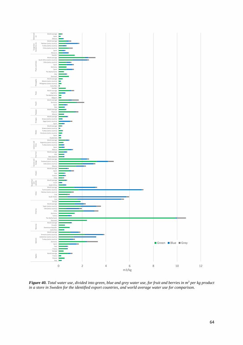
64

Figure 40. Total water use, divided into green, blue and grey water use, for fruit and berries in m3 per kg product

in a store in Sweden for the identified export countries, and world average water use for comparison.

0 2 4 6 8 10 12

Italy

Poland

France

World average

Sverige

France

Italy

Spain

Germany

Turkey (extra country)

Uzbekistan (extra country)

Armenia (extra country)

World average

Costa Rica

Dominican Republic

Ecuador

World average

Denmark

The Netherlands

Turkey

Germany

Chile

USA (extra country)

Spain (extra country)

World average

Sverige

Iran

Saudi Arabia

Iraq

Pakistan (extra country)

Tunisia (extra country)

World average

South Africa

Israel

World average

Chile

Greece

Italy

Spain

World average

Mexico

India (extra country)

Thailand (extra country)

World average

New Zealand

Italy

World average

Mexico

Spain

Turkey (extra country)

Argentina (extra country)

World average

Guatemala

Spain

Honduras (extra country)

Turkey (extra country)

Greece (extra country)

World average

Spain

Egypt (extra country)

Greece (extra country)

World average

Mexico

Thailand

World average

Italy

Spain

Germany

World average

Belgium

The Netherlands

Argentina

World average

Sweden

Costa Rica

Philippines (extra country)

Mexico (extra country)

World average

Denmark

Italy

The Netherlands

Spain

Germany

Spain

Chile (extra country)

South Africa (extra country)

World average

Sweden

Morocco

Spain

China (extra country)

Turkey (extra country)

Pakistan (extra country)

World average

Mexico

Spain

World averageA

pp

les

Ap

rico

tsB

anan

asC

he

rrie

sD

ates

Gra

pe

fru

itan

dp

om

elo

Gra

pe

sG

uav

as a

nd

man

goK

iwi f

ruit

Lem

on

s an

dlim

es

Mel

on

Ora

nge

sP

apay

asP

eac

hP

ear

sP

ine

app

les

Plu

ms

and

slo

es

Tan

geri

nes

man

dar

ins

etc

.W

ater

mel

on

m3/kg

Green Blue Grey

65

Figure 41. Total water use for fruit and berries in m3 per kg product.

Figure 42. Water use for fruits and berries assessed with the water scarcity method AWARE (Available Water

Remaining, m3eq per kg product), and the world average.

66

Table 19. Range of results for all identified export countries and Swedish produce for total water use (m3 per

functional unit (FU)) and AWARE (Available Water Remaining, m3eq per FU) for fruit and berries

Product Total water use

(m3 per FU)

AWARE (m3eq

per FU)

Commenta

Apples 0.2-1.2 0-8.7 Total water use for European production (including Swedish) is likely to be

0.5 m3 per kg. World average water use is higher, around 1.2 m3 per kg.

AWARE scores were highest for global average production.

Apricots 0.8-3.9 0.8-140 Total water use varies. It is highest for two of the extra countries (Armenia

and Uzbekistan) (see section 2.2), which also showed the highest AWARE

scores.

Bananas 0.5-1.1 0.3-24 Highest AWARE score found for the global average, the identified export

countries had lower scores.

Cherries 1.1-3.6 0.1-103 The Netherlands was excluded from the analysis. Total water use for

Swedish production is 1.9 m3 per kg and for the identified export counties

varies between 1.12-3.6 m3 per kg. Higher AWARE scores were found for

Spain and Chile.

Dates 1.0-7.2 0-910 Total water use varies greatly. Iraq, with the largest trade surplus globally,

has water use of 1 m3 per kg. In other identified export countries it varies

between 5.5-7.2 m3 per kg. The world average is lower, 3.3 m3 per kg,

indicating that total water use can be lower than for the identified export

countries. AWARE scores were found to be high for many of the countries.

AWARE scores close to zero are due to low irrigation rates.

Grapefruits

and pomelo

0.3-0.7 5.6-16 Total water use for global average and identified export countries was found

to be similar, 0.3-0.7 m3 per kg.

Grapes 0.5-1-3 0-10 Total water use for Chile, Greece, and Italy is relatively similar, below 0.6

m3 per kg. Spanish production has total water use of 1.3 m3 per kg. AWARE

scores are highest for Greece.

Guavas and

mango

2.3-4.7 7.5-24

Kiwi fruit 0.5-0.7 1.6-11 Similar water use for the main export countries, Italy and New Zealand (0.5

m3 per kg). Global average is similar (0.7 m3 per kg). Highest AWARE score

found for world average production.

Lemons and

limes

0.5-1.2 0.1-15 Total water use varies between 0.4-1.2 m3 per kg. Highest AWARE scores

found for Mexico and Spain.

Melons 0.2-0.4 0-6.0 For all identified export countries, total water use was assessed to be below

0.4 m3 per kg.

Oranges 0.2-1.2 7.2-82 Spain was identified as the main export country, with total water use of 0.5

m3 per kg. Highest AWARE score found for Egypt.

Papayas 0.5-1.7 0.7-3.4 Highest total water use is for produce from Thailand (1.7 m3 per kg),

Mexican export and global average is lower (0.5-0.7 m3 per kg).

Peaches 0.5-2.2 0.1-21 European production was assessed to have total water use of 0.5-2.2 m3 per

kg. The higher water use is for Germany. Highest AWARE score found for

Spain.

Pears 0.2-1.3 0-14 Total water use for the two identified European export countries was below

0.3 m3 per kg, for Swedish production 0.6 m3 per kg. Global average water

use is higher, indicating a risk of higher water use than the identified export

countries. Highest AWARE score found for Argentina.

Pineapples 0.1-0.4 0-1.2 Total water use for all export countries assessed is below 0.4 m3 per kg.

Plums and

sloes

0.5-3.1 0-48 Total water use varies between 0.5-3.1 m3 per kg. Swedish production has

water use around 1.4 m3 per kg. AWARE scores were highest for South

Africa, Spain, and Chile.

Tangerines and

mandarins

0.6-1.8 1.8-64 The two highest AWARE scores were found for Pakistan (extra country; see

section 2.2) and Morocco (main identified export country)

Watermelon 0.2-0.4 1.6-5.0

Berries

Cranberries 0-0.4 0-7.1 The USA was identified as the main export country, with total water use

estimated at 0.3 m3 per kg, similar to global average.

Blueberries

(cultivated)

0-2.5 0-22 Total water use is highest for Swedish blueberries (2.5 m3 per kg). Global

average has about half as high water use (1.2 m3 per kg) and Polish around

0.3 m3 per kg. In general, water use for imported blueberries is likely to be

below 1.2 m3 per kg. Highest AWARE score found for global average, all

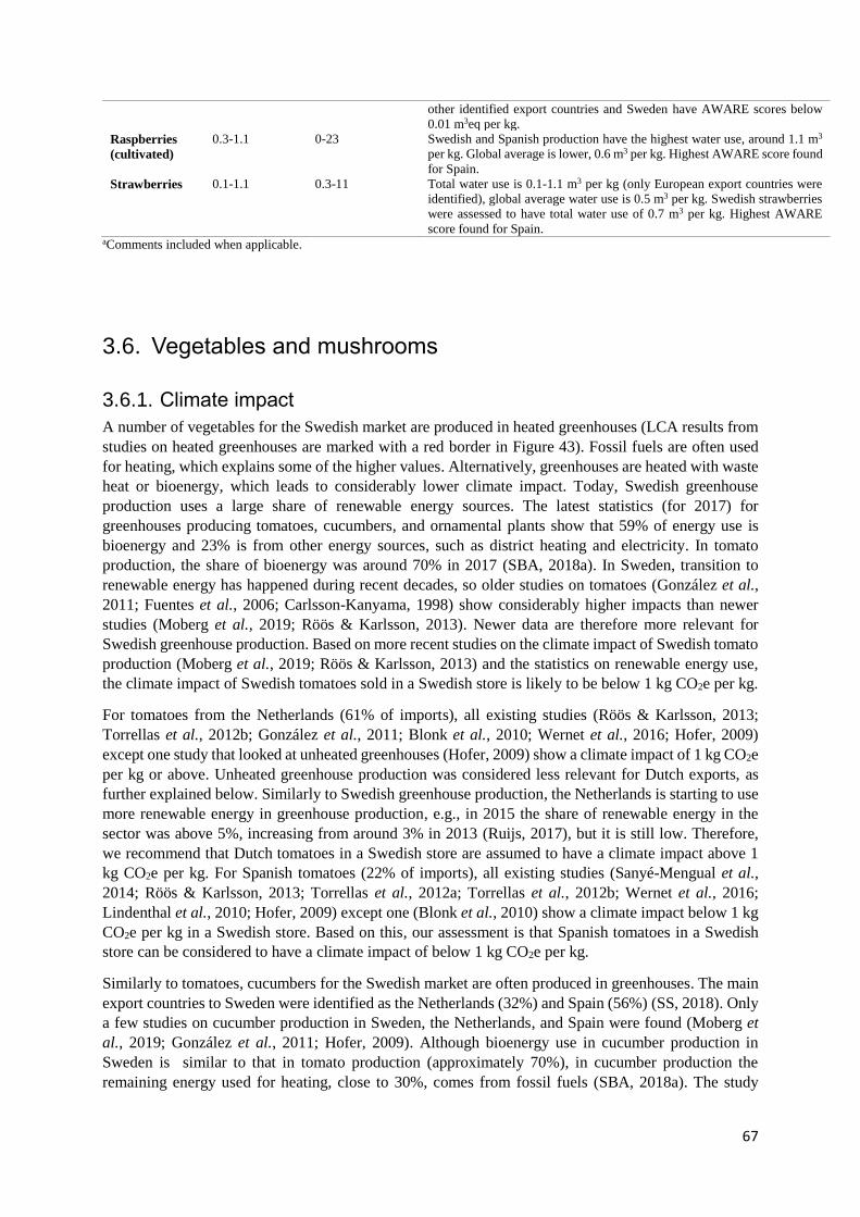
67

other identified export countries and Sweden have AWARE scores below

0.01 m3eq per kg.

Raspberries

(cultivated)

0.3-1.1 0-23 Swedish and Spanish production have the highest water use, around 1.1 m3

per kg. Global average is lower, 0.6 m3 per kg. Highest AWARE score found

for Spain.

Strawberries 0.1-1.1 0.3-11 Total water use is 0.1-1.1 m3 per kg (only European export countries were

identified), global average water use is 0.5 m3 per kg. Swedish strawberries

were assessed to have total water use of 0.7 m3 per kg. Highest AWARE

score found for Spain. aComments included when applicable.

3.6. Vegetables and mushrooms

3.6.1. Climate impact

A number of vegetables for the Swedish market are produced in heated greenhouses (LCA results from

studies on heated greenhouses are marked with a red border in Figure 43). Fossil fuels are often used

for heating, which explains some of the higher values. Alternatively, greenhouses are heated with waste

heat or bioenergy, which leads to considerably lower climate impact. Today, Swedish greenhouse

production uses a large share of renewable energy sources. The latest statistics (for 2017) for

greenhouses producing tomatoes, cucumbers, and ornamental plants show that 59% of energy use is

bioenergy and 23% is from other energy sources, such as district heating and electricity. In tomato

production, the share of bioenergy was around 70% in 2017 (SBA, 2018a). In Sweden, transition to

renewable energy has happened during recent decades, so older studies on tomatoes (González et al.,

2011; Fuentes et al., 2006; Carlsson-Kanyama, 1998) show considerably higher impacts than newer

studies (Moberg et al., 2019; Röös & Karlsson, 2013). Newer data are therefore more relevant for

Swedish greenhouse production. Based on more recent studies on the climate impact of Swedish tomato

production (Moberg et al., 2019; Röös & Karlsson, 2013) and the statistics on renewable energy use,

the climate impact of Swedish tomatoes sold in a Swedish store is likely to be below 1 kg CO2e per kg.

For tomatoes from the Netherlands (61% of imports), all existing studies (Röös & Karlsson, 2013;

Torrellas et al., 2012b; González et al., 2011; Blonk et al., 2010; Wernet et al., 2016; Hofer, 2009)

except one study that looked at unheated greenhouses (Hofer, 2009) show a climate impact of 1 kg CO2e

per kg or above. Unheated greenhouse production was considered less relevant for Dutch exports, as

further explained below. Similarly to Swedish greenhouse production, the Netherlands is starting to use

more renewable energy in greenhouse production, e.g., in 2015 the share of renewable energy in the

sector was above 5%, increasing from around 3% in 2013 (Ruijs, 2017), but it is still low. Therefore,

we recommend that Dutch tomatoes in a Swedish store are assumed to have a climate impact above 1

kg CO2e per kg. For Spanish tomatoes (22% of imports), all existing studies (Sanyé-Mengual et al.,

2014; Röös & Karlsson, 2013; Torrellas et al., 2012a; Torrellas et al., 2012b; Wernet et al., 2016;

Lindenthal et al., 2010; Hofer, 2009) except one (Blonk et al., 2010) show a climate impact below 1 kg

CO2e per kg in a Swedish store. Based on this, our assessment is that Spanish tomatoes in a Swedish

store can be considered to have a climate impact of below 1 kg CO2e per kg.

Similarly to tomatoes, cucumbers for the Swedish market are often produced in greenhouses. The main

export countries to Sweden were identified as the Netherlands (32%) and Spain (56%) (SS, 2018). Only

a few studies on cucumber production in Sweden, the Netherlands, and Spain were found (Moberg et

al., 2019; González et al., 2011; Hofer, 2009). Although bioenergy use in cucumber production in

Sweden is similar to that in tomato production (approximately 70%), in cucumber production the

remaining energy used for heating, close to 30%, comes from fossil fuels (SBA, 2018a). The study

68

considered most relevant for Swedish production was Moberg et al. (2019), due to its use of the most

recent data for heating.

Some high data-points for lettuce, pumpkin, and spinach are from a study lacking details of the inventory

and the results (Audsley et al., 2010), and therefore it is difficult to determine why the figures are much

higher than in other studies on the same crops. It is likely due to high fossil fuel use in greenhouses, but

this could not be confirmed.

Several studies on mushrooms were found (Robinson et al., 2019; Leiva et al., 2015; Ueawiwatsakul et

al., 2014; Tongpool & Pongpat, 2013; Gunady et al., 2012; Audsley et al., 2010; Blonk et al., 2010;

Maraseni et al., 2010). These studies focus on different types of mushrooms with large variation in the

climate impact. One of the most common mushroom types on the Swedish market is Agaricus bisporus

(Sw: trädgårdsschampinjon), which is the same type sold as portobello mushrooms (used as a substitute

for burgers, among other things). No study was found on production of mushrooms in the main exporting

countries to Sweden, which are Poland and Lithuania (SS, 2018). Three studies from other countries on

Agaricus bisporus were found (Robinson et al., 2019; Leiva et al., 2015; Gunady et al., 2012), with a

climate impact at farm gate varying from 2.1-4.4 kg CO2e per kg product. Climate control and the energy

use for this are important contributors to climate change for this type of production (Robinson et al.,

2019; Leiva et al., 2015), but also transport of substrate (manure and peat) (Gunady et al., 2012). There

is some commercial production of mushrooms in Sweden. However, no earlier study was found on this

production and no statistics on yearly production or yield were found.

Figure 43. Climate impact of vegetables and mushrooms in kg CO2e per kg product in a store in Sweden. The

squares represent earlier studies on products transported by air. Note that the graph shows the climate impact

from all identified earlier studies for this product group, and not only those identified as relevant for the Swedish

market. The final assessment in Table 20 is based on relevance for the Swedish market.

Table 20. Summary of recommendations for climate impact of vegetables and mushrooms on the Swedish market Product Final assessment

(kg CO2e per kg

product in a

Swedish store)

No. of

relevant

references

Total no.

of

references

Comment

General Sweden

69

Artichoke 0.6 1 1 European production considered most relevant for

the Swedish market. Only one study was found, so

the assessment is uncertain.

Asparagus 2.1 5 8 Final assessment is for European production. Three

studies show an impact below 1 kg CO2e per kg.

Import from the rest of the world carries a high risk

of air transport. Earlier studies show that the impact

can be as high as approx. 14 kg CO2e per kg product

(3 references).

Avocado 1.6 6 6 All identified studies considered relevant.

Broccoli 1.3 0.6 5 (2 SW) 8

Broccoli on the Swedish market is likely to originate

from southern Europe. Most studies show an impact

below or close to 1 kg CO2e per kg. However, two

studies show an impact above 1 kg CO2e per kg for

Spanish production, which is highly relevant for the

Swedish market. Climate impact for broccoli is

therefore likely to be below 1.3 kg CO2e per kg for

European production. Two studies were found on

Swedish production.

Cabbage 0.6 0.3 4 (3 SW) 7 European produce considered most relevant for the

Swedish market.

Capsicums/

peppers

1.5 2 7 Sweden imports come mainly from the Netherlands

and Spain, but no data were found for these

countries. Studies on European produce (Italian and

Swiss) were used for the final assessment.

Cauliflower

0.7 0.4 3 (1 SW) 6 European production considered relevant for the

final assessment. One study on European production

shows an impact above 2 kg CO2e per kg. However,

not enough detail is presented in that study to explain

the higher climate impact compared with other

studies, so it was not considered. Only one study was

found on Swedish production, this assessment is

uncertain.

Celery 0.6 0 3 European production considered most relevant for

the Swedish market. No study on European

production of celery was found. Considering the

LCA data found and the shorter transportation

distance, we estimated climate impact of celery for

the Swedish market based on production impact

from “rest of the world” (Australia, the USA and a

global average production) and general impact for

transport within Europe.

Cucumber 2.3 0.7 6 (2SW) 10 Often produced in heated greenhouses for the

Swedish market. Data on European production vary

greatly, mainly due to differences between heating

source for the greenhouses. Overall recommendation

based on earlier studies: European produce likely to

have a climate impact below 2 kg CO2e per kg, but

the impact can be lower, around 0.5 kg CO2e per kg,

depending mainly on greenhouse production or not,

and heating source. Products from outside Europe

are considered less relevant for the Swedish market.

Two relevant studies were found for the Swedish

market. This assessment is not valid for open field-

produced cucumbers grown in Sweden, such as

“västeråsgurka”.

Eggplant 1.7 2 6 European production considered relevant. The

higher impact is due to heated greenhouse.

Fennel 0.8 1 2 European production considered most relevant.

Garlic 0.8 2 3 European production considered most relevant. Only

one study was found on “rest of the world”

production, showing an impact of around 0.9 kg

CO2e per kg product.

Ginger 1.0 1 1 Only one study identified, the assessment is

uncertain.

70

Lettuce 0.7 0.4 7 (3 SW) 14 European production considered most relevant for

the final assessment. Assessment based on open field

production for iceberg lettuce, for both European and

Swedish production. Fresh lettuce sold in pots can be

cultivated in heated greenhouses and therefore

associated with substantially higher climate impact.

Green beans 0.8 2 5 European production considered most relevant. This

assessment included one study on frozen green

beans. One study on European green beans was not

considered, since it showed much higher climate

impact than the other studies and did not explain the

processes in detail. Further, canned green beans were

considered less relevant for the Swedish market. For

green beans imported from outside Europe, there is

a risk of air transport. One earlier study was found

on green beans transported from Kenya and Uganda

with a total climate impact of 9.7-10.1 kg CO2e per

kg product.

Olives 1.0 4 5 European production considered most relevant. One

study on European olives was excluded, due to much

higher climate impact and insufficient data in the

report to evaluate the figure.

Onions 1.0 0.3 8 (4 SW) 8 All studies considered relevant. European

production likely below 0.8 kg CO2e per kg onions

(6 references).

Pumpkins

and squash

0.13 1 3 European studies considered most relevant for the

Swedish market. One study on European production

was excluded due to much higher climate impact and

insufficient amount of data in the report to evaluate

the figure. The assessment is based on one study, and

is therefore uncertain.

Spinach 0.5 1 5 European studies considered most relevant for the

Swedish market. One study on European production

was excluded. One study on European spinach was

excluded due to much higher climate impact and

insufficient data to evaluate the figure. The

assessment is based on one study and is therefore

uncertain. However, this study has a result similar to

the studies on “rest of the world” production.

Tomatoes 2.3 0.9 17 (2 SW) 28 Fresh tomatoes on the Swedish market are likely to

originate from within Europe. Climate impact varies

greatly, the main reason being the heating source for

the greenhouses. The most recent study on Swedish

tomatoes shows a climate impact of around 0.9 kg

CO2e per kg. Data for European production varies

greatly. Clearly many of the data-points are below 1

kg CO2e per kg. Some show impacts of around 6 kg

CO2e per kg, but often older studies, and the energy

mix for heating has changed greatly in Sweden over

time. In summary, earlier studies show that tomatoes

produced in Europe are likely to have a climate

impact below 2.3 kg CO2e per kg or in many cases

much lower. However, the climate impact can be

higher, depending on heating source for heating the

greenhouses. Sweden mostly imports tomatoes from

Spain and the Netherlands. Spanish tomatoes are

likely to have climate impact below 1 kg CO2e per

kg, Dutch tomatoes are likely to have climate impact

below 2.3 kg CO2e per kg in a store in Sweden.

Mushrooms 4.7 3 8 Sweden imports mushrooms mainly from Europe.

No study on production of Agaricus bisporus (Sw:

trädgårdsschampinjon) from the identified export

countries was found. Studies on Agaricus bisporus

show a climate impact of 2.5-4.7 kg CO2e per kg

product. Climate impact is therefore considered to be

below 4.7 kg CO2e per kg product. Earlier studies

indicate that climate control and the energy source

71

for this can be important (similar to greenhouse

production) (3 references)

3.6.2. Land use

For most vegetables, land use was assessed to be below 2 m2 per kg product. Artichokes, asparagus, and

avocados can be associated with higher land use than 2 m2 (Figure 44). Olives from all countries of

origin assessed had higher land use, 4-9 m2 (global average), due to low yields.

The biodiversity assessment (Figure 45) showed that asparagus from Mexico, avocados from Mexico

and Peru, and peppers from Mexico and olives from Greece and Spain risk having a higher impact on

biodiversity than the other products in the vegetables and mushrooms category.

Figure 44. Land use for vegetables and mushrooms in m2 per kg in a store in Sweden, and the global average.

3.6.3. Biodiversity

In this product group, biodiversity impact was highest for avocados, olives, and asparagus from Mexico

and Peru, and peppers from Mexico, due to high land use for these products in combination with high

biodiversity in the areas where they are produced.

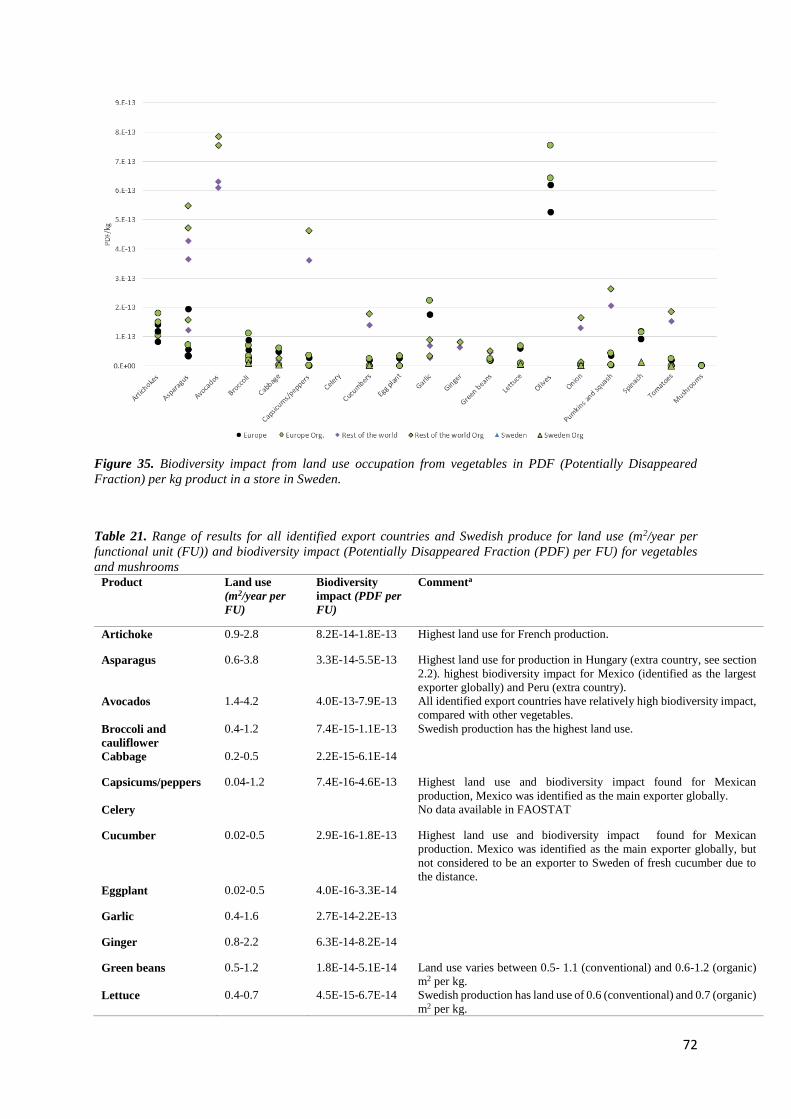
72

Figure 35. Biodiversity impact from land use occupation from vegetables in PDF (Potentially Disappeared

Fraction) per kg product in a store in Sweden.

Table 21. Range of results for all identified export countries and Swedish produce for land use (m2/year per

functional unit (FU)) and biodiversity impact (Potentially Disappeared Fraction (PDF) per FU) for vegetables

and mushrooms Product Land use

(m2/year per

FU)

Biodiversity

impact (PDF per

FU)

Commenta

Artichoke 0.9-2.8 8.2E-14-1.8E-13 Highest land use for French production.

Asparagus 0.6-3.8 3.3E-14-5.5E-13 Highest land use for production in Hungary (extra country, see section

2.2). highest biodiversity impact for Mexico (identified as the largest

exporter globally) and Peru (extra country).

Avocados 1.4-4.2 4.0E-13-7.9E-13 All identified export countries have relatively high biodiversity impact,

compared with other vegetables.

Broccoli and

cauliflower

0.4-1.2 7.4E-15-1.1E-13 Swedish production has the highest land use.

Cabbage 0.2-0.5 2.2E-15-6.1E-14

Capsicums/peppers 0.04-1.2 7.4E-16-4.6E-13 Highest land use and biodiversity impact found for Mexican

production, Mexico was identified as the main exporter globally.

Celery No data available in FAOSTAT

Cucumber 0.02-0.5 2.9E-16-1.8E-13 Highest land use and biodiversity impact found for Mexican

production. Mexico was identified as the main exporter globally, but

not considered to be an exporter to Sweden of fresh cucumber due to

the distance.

Eggplant 0.02-0.5 4.0E-16-3.3E-14

Garlic 0.4-1.6 2.7E-14-2.2E-13

Ginger 0.8-2.2 6.3E-14-8.2E-14

Green beans 0.5-1.2 1.8E-14-5.1E-14 Land use varies between 0.5- 1.1 (conventional) and 0.6-1.2 (organic)

m2 per kg.

Lettuce 0.4-0.7 4.5E-15-6.7E-14 Swedish production has land use of 0.6 (conventional) and 0.7 (organic)

m2 per kg.

73

Olives 4.0-9.3 5.3E-13-7.5E-13 Higher land use value for both conventional and organic production is

global average.

Onions 0.1-1.2 2.0E-15-1.6E-13 Swedish production has land use of 0.2 (conventional) and 0.3 (organic)

m2 per kg.

Pumpkins and

squash

0.2-1.0 3.2E-15-2.6E-13 Highest biodiversity impact for Mexican production, Mexico was

identified as the main exporter globally.

Spinach 0.4-1.7 1.0E-14-1.2E-13 Swedish production has land use of 1.3 (conventional) and 1.7 (organic)

m2 per kg.

Tomatoes 0.02-0.5 3.2E-16-1.9E-13 Swedish production has land use of 0.03 (conventional) and 0.04

(organic) m2 per kg. Highest biodiversity impact found for Mexican

production, Mexico was identified as the main exporter globally.

Highest biodiversity impact for European production found for Spanish

production.

Mushrooms 0.04-0.06 5.3E-16-8.7E-16

a Comments included when applicable.

3.6.4. Water use

Earlier studies

Blue water use is included in several earlier studies on vegetables (Appendix A1). The highest water

use is reported for asparagus and avocados.

Figure 46. Blue water use in earlier studies for vegetables and mushrooms.

Own assessment

Olives, ginger (world average production), asparagus, avocados, and artichokes are the crops within the

category ‘Vegetables and mushrooms’ that have the highest total water use (Figures 47 and 48).

Generally, the use of irrigation (blue water) is also high for these crops (Mekonnen et al., 2011). World

average production and the selected export countries have similar water use for all crops except ginger,

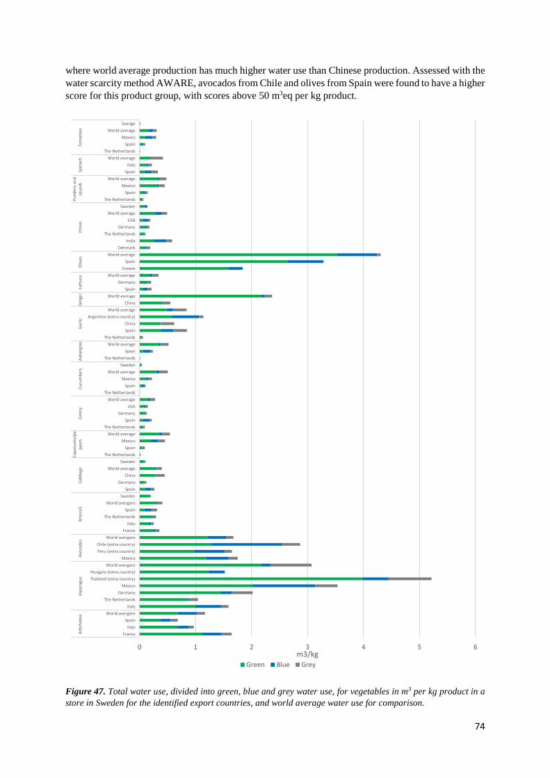
74

where world average production has much higher water use than Chinese production. Assessed with the

water scarcity method AWARE, avocados from Chile and olives from Spain were found to have a higher

score for this product group, with scores above 50 m3eq per kg product.

Figure 47. Total water use, divided into green, blue and grey water use, for vegetables in m3 per kg product in a

store in Sweden for the identified export countries, and world average water use for comparison.

0 1 2 3 4 5 6

France

Italy

Spain

World avergare

Italy

The Netherlands

Germany

Mexico

Thailand (extra country)

Hungary (extra country)

World avergare

Mexico

Peru (extra country)

Chile (extra country)

World avergare

France

Italy

The Netherlands

Spain

World avergare

Sweden

Spain

Germany

China

World average

Sweden

The Netherlands

Spain

Mexico

World average

The Netherlands

Spain

Germany

USA

World average

The Netherlands

Spain

Mexico

World average

Sweden

The Netherlands

Spain

World average

The Netherlands

Spain

China

Argentina (extra country)

World average

China

World average

Spain

Germany

World average

Greece

Spain

World average

Denmark

India

The Netherlands

Germany

USA

World average

Sweden

The Netherlands

Spain

Mexico

World average

Spain

Italy

World average

The Netherlands

Spain

Mexico

World average

Sverige

Art

ich

oke

sA

spar

agu

sA

voca

dos

Bro

cco

liC

abb

age

Cap

sicu

ms/

pe

pp

ers

Cel

ery

Cu

cum

ber

sA

ub

ergi

ne

Gar

licG

inge

rLe

ttu

ceO

lives

On

ion

Pu

mki

ns

and

squ

ash

Spin

ach

Tom

ato

es

m3/kgGreen Blue Grey

75

Figure 48. Total water use for vegetables in m3 per kg product.

Figure 49. Water use for vegetables and mushrooms assessed with the water scarcity method AWARE (Available

Water Remaining, m3eq per kg product) in a store in Sweden, and world average.

Table 22. Range of results for all identified export countries and Swedish produce for total water use (m3 per

functional unit (FU)) and AWARE (Available Water Remaining, m3eq per FU) for vegetables and mushrooms

76

Product Total water

use (m3 per

FU)

AWARE (m3eq

per FU)

Commentsa

Artichokes 0.7-1.7 2.9-16 Highest AWARE score found for Spanish production.

Asparagus 1.0-5.2 0.5-39 Highest AWARE score found for Mexico, the country identified as the

main exporter globally, but not to Sweden (not appearing in import

statistics).

Avocados 1.7-2.9 14-100 Mexico, Peru, and world average production have similar water use,

below 1.8 m3. Avocados from Chile were assessed to have water use of

around 2.9 m3 per kg product. Chile also has the highest AWARE score

for avocado production.

Broccoli and

cauliflower

0.2-0.4 0-10 Water use for identified export countries, Swedish production and world

average production is similar, total water use for these crops is likely to

be below 0.4 m3. Highest AWARE score found for Spanish production.

Cabbage 0.1-0.4 0.02-8.3 Highest AWARE score found for Spain.

Capsicums/peppers 0.02-0.5 0-4.4

Celery 0.1-0.3 0.1-8.6 Highest AWARE score found for Spain.

Cucumber 0.1-0.5 0-3.0 Highest AWARE score found for Spain.

Eggplant 0.01-0.5 0-10 Highest AWARE score found for Spain.

Garlic 0.1-1.1 0-27 Spanish and world average production had total water use of 1 m3.

Highest AWARE scores found for Argentina (extra country) and Spain

(one of the identified export countries).

Ginger 0.6-2.4 0.8-2.6 China was identified as the main exporter, with water use of 0.6 m3.

World average production has much higher water use, 2.4 m3, indicating

a risk of higher water use than the main export country.

Lettuce 0.2-0.3 0-6.9 Highest AWARE score found for Spain.

Olives 1.8-4.3 18-51 Total water use in the main exporting country (Spain with 54% of

Swedish imports) was estimated to be 3.3 m3. World average production

4.3 m3. AWARE scores were found to be relatively high.

Onions 0.1-0.6 0.01-6.8 Total water use for Swedish production was assessed to be 0.1 m3.

Imported onions from European countries generally have water use

below 0.2 m3. India (identified as one of the export countries and the

largest exporter globally) has the highest total water use and highest

AWARE score for onions.

Pumpkins and

squash

0.1-0.5 0-3.1 The Netherlands and Spain were identified as main export countries in

Europe, total water use was assessed to be below 0.14 m3. Mexico is the

largest exporter globally, with water use similar to the global average,

below 0.5 m3. Highest AWARE score found for Spain.

Spinach 0.2-0.4 1.0-11 Spain, Italy, and world average have similar total water use of below 0.4

m3. Highest AWARE score found for Spain.

Tomatoes 0.01-0.3 0-4.6 Sweden and the Netherlands have similar water use for tomato

production, approx. 0.01 m3. Spanish production uses around 0.1 m3 and

Mexican production and world average production 0.3 m3.

Mushrooms No data

a Comments included when applicable.

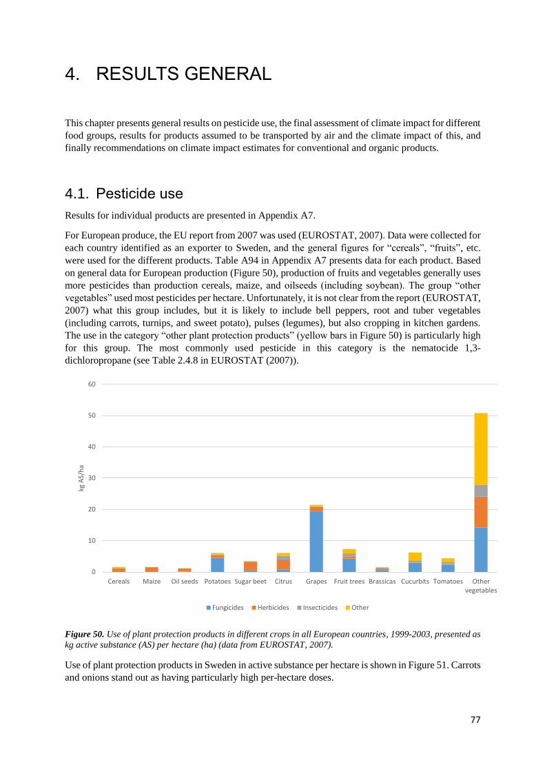
77

4. RESULTS GENERAL

This chapter presents general results on pesticide use, the final assessment of climate impact for different

food groups, results for products assumed to be transported by air and the climate impact of this, and

finally recommendations on climate impact estimates for conventional and organic products.

4.1. Pesticide use

Results for individual products are presented in Appendix A7.

For European produce, the EU report from 2007 was used (EUROSTAT, 2007). Data were collected for

each country identified as an exporter to Sweden, and the general figures for “cereals”, “fruits”, etc.

were used for the different products. Table A94 in Appendix A7 presents data for each product. Based

on general data for European production (Figure 50), production of fruits and vegetables generally uses

more pesticides than production cereals, maize, and oilseeds (including soybean). The group “other

vegetables” used most pesticides per hectare. Unfortunately, it is not clear from the report (EUROSTAT,

2007) what this group includes, but it is likely to include bell peppers, root and tuber vegetables

(including carrots, turnips, and sweet potato), pulses (legumes), but also cropping in kitchen gardens.

The use in the category “other plant protection products” (yellow bars in Figure 50) is particularly high

for this group. The most commonly used pesticide in this category is the nematocide 1,3-

dichloropropane (see Table 2.4.8 in EUROSTAT (2007)).

Figure 50. Use of plant protection products in different crops in all European countries, 1999-2003, presented as

kg active substance (AS) per hectare (ha) (data from EUROSTAT, 2007).

Use of plant protection products in Sweden in active substance per hectare is shown in Figure 51. Carrots

and onions stand out as having particularly high per-hectare doses.

0

10

20

30

40

50

60

Cereals Maize Oil seeds Potatoes Sugar beet Citrus Grapes Fruit trees Brassicas Cucurbits Tomatoes Othervegetables

kg A

S/h

a

Fungicides Herbicides Insecticides Other

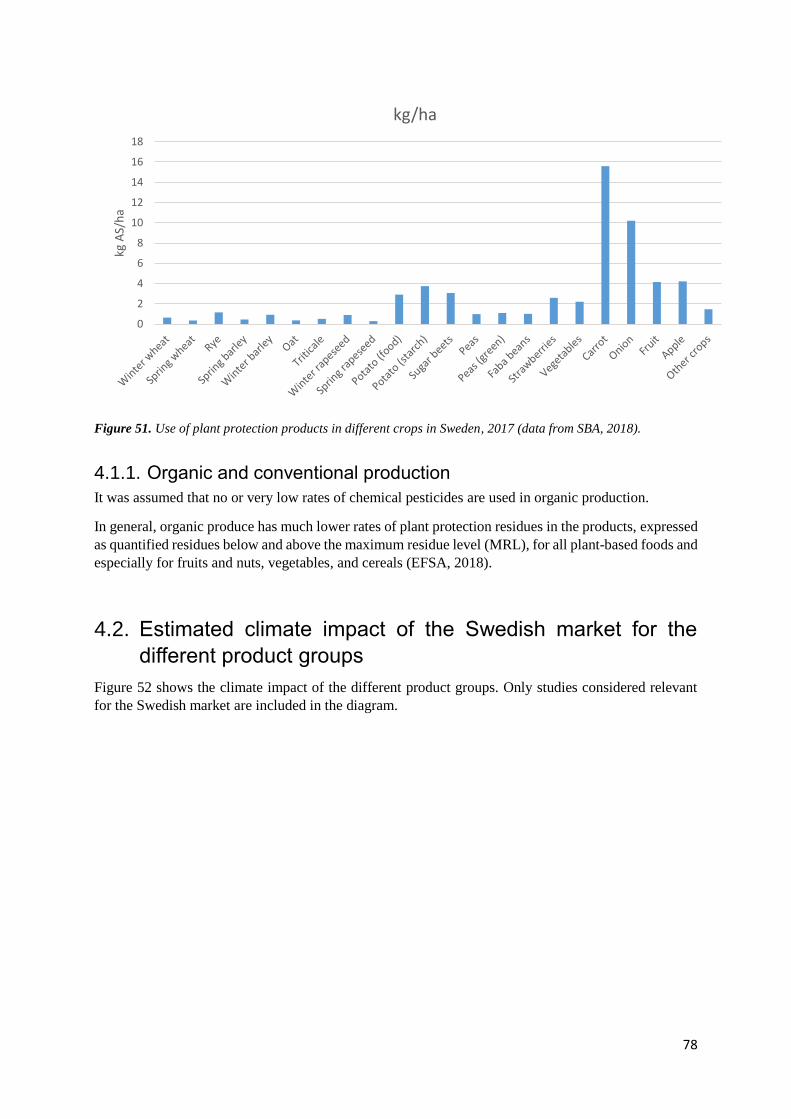
78

Figure 51. Use of plant protection products in different crops in Sweden, 2017 (data from SBA, 2018).

4.1.1. Organic and conventional production

It was assumed that no or very low rates of chemical pesticides are used in organic production.

In general, organic produce has much lower rates of plant protection residues in the products, expressed

as quantified residues below and above the maximum residue level (MRL), for all plant-based foods and

especially for fruits and nuts, vegetables, and cereals (EFSA, 2018).

4.2. Estimated climate impact of the Swedish market for the

different product groups

Figure 52 shows the climate impact of the different product groups. Only studies considered relevant

for the Swedish market are included in the diagram.

0

2

4

6

8

10

12

14

16

18

kg A

S/h

akg/ha

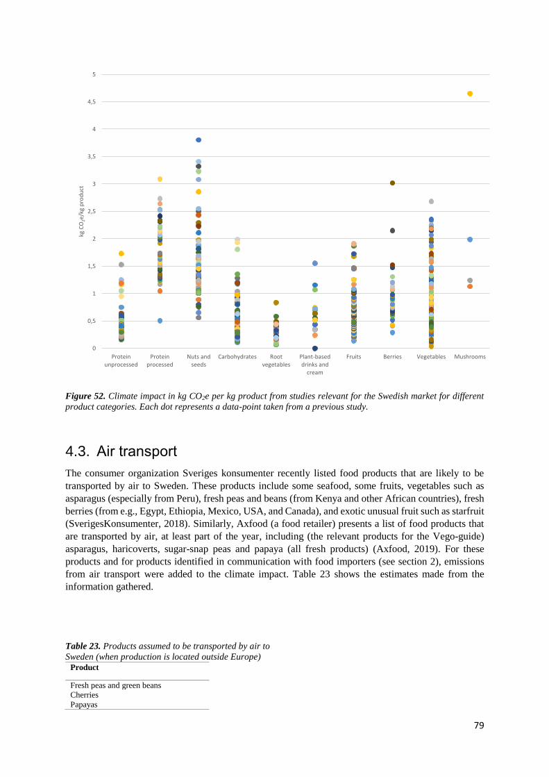
79

Figure 52. Climate impact in kg CO2e per kg product from studies relevant for the Swedish market for different

product categories. Each dot represents a data-point taken from a previous study.

4.3. Air transport

The consumer organization Sveriges konsumenter recently listed food products that are likely to be

transported by air to Sweden. These products include some seafood, some fruits, vegetables such as

asparagus (especially from Peru), fresh peas and beans (from Kenya and other African countries), fresh

berries (from e.g., Egypt, Ethiopia, Mexico, USA, and Canada), and exotic unusual fruit such as starfruit

(SverigesKonsumenter, 2018). Similarly, Axfood (a food retailer) presents a list of food products that

are transported by air, at least part of the year, including (the relevant products for the Vego-guide)

asparagus, haricoverts, sugar-snap peas and papaya (all fresh products) (Axfood, 2019). For these

products and for products identified in communication with food importers (see section 2), emissions

from air transport were added to the climate impact. Table 23 shows the estimates made from the

information gathered.

Table 23. Products assumed to be transported by air to

Sweden (when production is located outside Europe) Product

Fresh peas and green beans

Cherries

Papayas

0

0,5

1

1,5

2

2,5

3

3,5

4

4,5

5

Proteinunprocessed

Proteinprocessed

Nuts andseeds

Carbohydrates Rootvegetables

Plant-baseddrinks and

cream

Fruits Berries Vegetables Mushrooms

kg C

O2e/

kg p

rod

uct

80

Asparagus

Table 24 presents climate impact of air transport of 1 kg from five different countries (from each

country’s capital to Stockholm). The climate impact was calculated using NTMCalc and additional

climate impact from emitting greenhouse gases at high altitudes is not taken into account (NTM, 2019),

but could double the climate impact caused by the emissions.

Table 24. Climate impact of air transport from relevant countries Country of origin kg CO2e per kg

transported to Sweden

Canada 4.0

Chile 8.0

Egypt 2.5

Ethiopia 3.8

Guatemala 6.0

Honduras 5.9

India 3.6

Kenya 4.2

Mexico 5.9

Morocco 2.3

New Zealand 10.6

Peru 7.1

South Africa 5.9

Thailand 5.2

Turkey 2.1

USA 4.2

Earlier studies sometimes include air transport of fresh vegetables. For example, i Canals et al. (2008)

assessed the climate impact of fresh green beans transported by air from Kenya and Uganda to the UK,

and found it to be 10.7-10.9 kg CO2e per kg product.

4.4. Climate impact of conventional and organic products

There are numerous LCA studies of both conventional and organic production systems. When reviewing

earlier studies on climate impact and energy use, we did not differentiate between these two systems,

but analyzed these studies jointly. Previous studies show that organic systems have similar climate

impact to organic systems (Clark & Tilman, 2017).

81

5. DISCUSSION

5.1. Data availability

Rapid product development for plant-based ready-made protein sources is underway, but studies on the

environmental impact are not available for all such products. As more products are introduced, it is

likely that more studies on their environmental impact will emerge in the near future. There might

therefore be a need to update the underlying data for the Vego-guide in coming years, to include new

studies on the products included, but also to include a wider variety of products. For example, in this

report an attempt is made to include plant-based cheese and deli meat. However, previous studies on the

environmental impact of these products are very scarce.

Assessments on the likely climate impact of different products on the Swedish market were based on

earlier studies and an assessment made by the authors on which of these are most representative for the

Swedish market. For several products there are few studies, and in several cases no studies, on

production in the identified export countries. In these situations, the final assessment was based on the

available data and it was noted that the assessment was made with little access to representative data.

To determine common country of origin of the products, trade statistics were used. A well-known issue

with trade statistics is that the country of origin is not always the country of primary production, as the

countries listed as export countries in the statistics sometimes does not have any primary production of

the product. For example, the Netherlands appears often as an export country, since it is a trade hub. In

addition to the use of trade statistics, we tried to retrieve data on country of origin from wholesalers that

primarily import fruits and vegetables. However, we were unable to verify our import data through

information from wholesalers (Lundmark, 2019).

Data on pesticide use are particularly scarce, as is access to relevant and reliable indicators on ecotoxicity

of pesticide use. The data used for European production are relatively old (from 2007), but no more

recent data could be found. EUROSTAT includes data on pesticide use in the different countries, but

we could not find a way to link this use to specific crops. In order to evaluate pesticide use, there is a

need for better data which can be linked to different crops.

5.2. Methodological discussion

While emissions of greenhouse gases have the same impact on the climate no matter where they are

emitted, the use of land in different regions of the world will have different impacts on biodiversity and

the use of water will have different impacts on regional water availability. For the biodiversity impact

assessment method (Chaudhary et al., 2018) and water scarcity method (Boulay et al., 2018), country

average characterization methods were used, although both of these methods provide characterization

factors for smaller regions than countries. The primary reason for using country average characterization

factors was that import statistics do not report the region/s of a country in which products are produced.

The assessment of products from large countries was likely to have been particularly affected by this,

e.g., almonds from Spain and the USA. Almonds produced in the USA are likely to originate from

California, which has a higher characterization factor for biodiversity loss due to land use than the

average for agricultural land in USA. This means that growing almonds in California is likely to be

associated with higher biodiversity loss than growing them on an average field in the USA. However,

we used the characterization factor for the whole USA, to be consistent with using country average

characterization factors for all imported products. Our results show that almonds from Spain are

82

associated with higher biodiversity loss due to land occupation than almonds from USA. This is due to

Spanish production being associated with higher land use, but also to the characterization factor for

Spain being higher than that for the USA. In this comparison, a smaller country like Spain has a higher

factor since most of the country has a more tropical climate than the overall USA.

Total water use was assumed to be the same for organic and conventional produce. Total water use

information was retrieved from the water footprint network (Mekonnen et al., 2011), where green, blue,

and grey water use in an area is distributed over the yield of that area, based on FAO statistics.

Considering that conventional agriculture is likely to be the dominant form of agriculture in most

countries, the average FAOSTAT yield is likely to be more representative of conventional production.

Assuming that water use is the same for conventional and organic production therefore risks

underestimation of the water use for organic production, as it is often associated with lower yields. The

lower yields in organic agriculture were accounted for in our land use and biodiversity assessments.

83

REFERENCES

Agri-footprint (2018). Agri-footprint 4.0. Gouda, the Netherlands.

Hoekstra Y.A., Chapagain, A.K., Aldaya, M.M. & Mekonnen, M.M. (2012). The water footprint

assessment manual: Setting the global standard. Earthscan. London, UK. Washington DC,

USA.

Alter eco (2012). 2012 EMISSIONS REPORT & IMPACT ASSESSMENT.

http://www.alterecofoods.com/reports/AlterEco-Emissions Report-2012.pdf (accessed:

20190217).

Audsley, E., Brander, M., Chatterton, J., Murphy-Bokern, D., Webster, C., Williams, A.J.G., (2009). An

assessment of greenhouse gas emissions from the UK food system and the scope for reduction

by 2050: how low can we go. UK: WWF UK & Network, F.C.R.

Axfood (2020). Axfoods insatser för minskad klimatpåverkan. https://www.axfood.se/hallbarhet/sa-

jobbar-vi/klimat-och-energi/ (accessed: 20200601).

Bartzas, G., Vamvuka, D. & Komnitsas, K. (2017). Comparative life cycle assessment of pistachio,

almond and apple production, Information Processing in Agriculture, 4(3), pp. 188-198.

Blengini, G.A. & Busto, M. (2009). The life cycle of rice: LCA of alternative agri-food chain

management systems in Vercelli (Italy), Journal of Environmental Management, 90(3), pp.

1512-1522.

Blonk, H., Kool, A., Luske, B., de Waart, S. (2008). Environmental effects of protein-rich food products

in the Netherlands Consequences of animal protein substitutes. Blonk Milieuadvies, Gouda.

Nederlandse Vegetariërsbond.

Blonk, H., Kool, A., Luske, B., Ponsioen, T. & Scholten, J. (2010). Methodology for assessing carbon

footprints of horticultural products. Milieueffecten van vlees en vleesvervangers. Eindrapport v

1.2. Blonk consultans (2017).

Bognár, A. (2002). Tables on weight yield and retention factors of food constituents for the calculation

of nutrient composition of cooked foods (dishes). (Bundesforschungsanstalt für Ernährung).

Karlsruhe, Germany.

Boulay, A.-M., Bare, J., Benini, L., Berger, M., Lathuillière, M.J., Manzardo, A., Margni, M., Motoshita,

M., Núñez, M. Pastor, A.V., Ridoutt, B., Oki, T., Worbe, S. & Pfister, S. (2018). The WULCA

consensus characterization model for water scarcity footprints: assessing impacts of water

consumption based on available water remaining (AWARE), The International Journal of Life

Cycle Assessment, 23(2), pp. 368-378.

Brenton, P., Edwards-Jones, G. & Jensen, M.F. (2010). Carbon footprints and food systems: do current

accounting methodologies disadvantage developing countries?: A World Bank study.

Washington, D.C. : World Bank Group.

Broekema, R. & Blonk, H. (2009). Milieukundige vergelijking van vleesvervangers. Blonk

Milieuadvies. Gouda, The Netherlands.

Cancino-Espinoza, E., Vázquez-Rowe, I. & Quispe, I. (2018). Organic quinoa (Chenopodium quinoa

L.) production in Peru: Environmental hotspots and food security considerations using Life

Cycle Assessment, Science of the Total Environment, 637, pp. 221-232.

Carlsson-Kanyama, A. (1998). Climate change and dietary choices—how can emissions of greenhouse

gases from food consumption be reduced? Food Policy, 23(3-4), pp. 277-293.

Carlsson-Kanyama, A. & Faist, M. (2000). Energy Use in the Food Sector: A data survey. Swedish

Environment Protection Agency. AFN report 291. Stockholm, Sweden.

Cellura, M., Ardente, F. & Longo, S. (2012). From the LCA of food products to the environmental

assessment of protected crops districts: a case-study in the south of Italy. Journal of

Environmental Management, 93(1), pp. 194-208.

Chaudhary, A. & Brooks, T. M. (2018). Land Use Intensity-Specific Global Characterization Factors to

Assess Product Biodiversity Footprints. Environemntal Science and Technology 52(9), pp.

5094-5104.

84

Chaudhary, A., Verones, F., de Baan, L. &Hellweg, S. (2015). Quantifying land use impacts on

biodiversity: combining species–area models and vulnerability indicators. Environemntal

Science and Technology , 49(16), pp. 9987-9995.

Clark, M. & Tilman, D. (2017). Comparative analysis of environmental impacts of agricultural

production systems, agricultural input efficiency, and food choice. Environemntal Research

Letters 12(6), p. 064016.

Clune, S., Crossin, E. & Verghese, K.J. (2017). Systematic review of greenhouse gas emissions for

different fresh food categories, Journal of Cleaner Production. 140, pp. 766-783.

de Baan, L., Alkemade, R. & Koellner, T. (2012). Land use impacts on biodiversity in LCA: a global

approach. The International Journal of Life Cycle Assessment, pp. 1-15.

De Ponti, T., Rijk, B. & Van Ittersum, M.K. (2012). The crop yield gap between organic and

conventional agriculture, Agricultural systems, 108, pp. 1-9.

EFSA. (2018). The 2016 European Union report on pesticide residues in food. European Food Safety

Authority. doi: 10.2903/j.efsa.2018.5348.

Ekqvist, I., Röös, E. & Tidåker, P. (2019). Grain legumes on the Swedish market: origin and pesticide

use in the production. Report 108. Department of energy and technology, SLU, Uppsala.

EUROSTAT (2007). The use of plant protection products in the European Union Data 1992-2003.

European Communities.

FAO (2017). Water for Sustainable Food and Agriculture A report produced for the G20 Presidency of

Germany. Food and Agriculture Organization of the United Nations. Rome, Italy.

FAO (year unknown). Almond production. http://www.fao.org/3/x5337e/x5337e02.htm (accessed:

2020-04-06).

FAOSTAT (2019). Statistic database. Food and Agricultural Organization of the United Nations.

Finnigan, T., Lemon, M., Allan, B. & Paton, I. (2010). Mycoprotein, Life cycle Analysis and the food

2030 challenge. Aspects of Applied Bioenergy, (102), pp. 81-90.

Finnigan, T., Needham, L. & Abbott, C. (2017). Mycoprotein: a healthy new protein with a low

environmental impact. In: Sustainable protein sources. Elsevier, pp. 305-325.

Florén, B., Nilsson, K. & Wallman, M. (2013). LCA på färsk och aseptiskt havredryck. Confidential

report PX20462.

Foster, C., Guében, C., Holmes, M., Wiltshire, J. & Wynn, S. (2014). The environmental effects of

seasonal food purchase: a raspberry case study. Journal of cleaner production, 73, pp. 269-274.

Fraanje, W. & Garnet, T. (2020). Soy: food, feed, and land use change (Foodscource: Building Blocks).

Food Climate Research Network, University of Oxford.

Fuentes, C. & Carlsson-Kanyama A. (eds.); Biel, A., Bergström, K., Carlsson- Kanyama, A., Fuentes,

C., Grankvist, G., Lagerberg Fogelberg, C.,Shanahan H. & Solér, C. (2006). Environmental

information in the food supply system. FOI, Swedish Defence Research Agency, Stockholm,

Sweden.

Fulton, J., Norton, M. & Shilling, F. (2018). Water-indexed benefits and impacts of California almonds.

Ecological Indicators, 96 part 1, pp. 711-717.

González, A.D., Frostell, B. & Carlsson-Kanyama, A. Protein efficiency per unit energy and per unit

greenhouse gas emissions: potential contribution of diet choices to climate change mitigation,

Food policy, 36(5), pp. 562-570.

Gunady, M.G., Biswas, W., Solah, V.A. & James, A.P. (2012). Evaluating the global warming potential

of the fresh produce supply chain for strawberries, romaine/cos lettuces (Lactuca sativa), and

button mushrooms (Agaricus bisporus) in Western Australia using life cycle assessment (LCA).

Journal of Cleaner Production, 28, pp. 81-87.

Gustavsson, J., Cederberg, C., Sonesson, U., van Otterdijk, R. & Meybeck, A. (2011). Global food losses

and food waste. Food and Agriculture Organization of the United Nations. Rome, Italy.

Head, M., Sevenster, M.N. & Croezen, H. (2011). Life cycle impacts of protein-rich foods for

superwijzer. Publication number 11.2329.57, CE Delft.

Henderson, A. & Unnasch, S. (2017). Life Cycle Assessment of Ripple Non-Dairy Milk. Life cycle

associates, LLC. Report number LCA.6121.159.2017.

Hofer, B. (2009) How to reduce the environmental footprint of consumer goods: LCA studies on fruit

and vegetables production. In: Proceedings of Coop Switzerland, 37th LCA Discussion Forum,

Lausanne 2009.

85

Hushållningssällskapet (2013). Alternativa livsmedelsgrödor. HS konsult AB, Uppsala, Sweden.

i Canals, L.M., Muñoz, I., Hospido, A., Plassmann, K., McLaren, S., Edwards-Jones, G. & Hounsome,

B. (2008). Life Cycle Assessment (LCA) of domestic vs. imported vegetables. Case studies on

broccoli, salad crops and green beans. CES Working Paper 01/08.

IPBES (2019). IPBES (2019). Summary for policymakers of the global assessment report on biodiversity

and ecosystem services. The Intergovernmental Science‐Policy Platform on Biodiversity and

Ecosystem Services. Jolliet, O., Antón, A., Boulay, A.-M., Cherubini, F., Fantke, P., Levasseur, A., McKone, T.E.,

Michelsen, O., i Canals, L.M. & Motoshita, M. (2018). Global guidance on environmental life

cycle impact assessment indicators: impacts of climate change, fine particulate matter

formation, water consumption and land use. The International Journal of Life Cycle Assessment,

23(11), pp. 2189-2207.

Kendall, A. & Brodt, S.B. (2014) Comparing alternative nutritional functional units for expressing life

cycle greenhouse gas emissions in food production systems. In: Proceedings of Proceedings of

the 9th International Conference on Life Cycle Assessment in the Agri-Food Sector (LCA Food

2014), San Francisco, California, USA, 8-10 October, 2014.

Kool, A., Marinussen, M. & Blonk, H. (2012). LCI data for the calculation tool Feedprint for

greenhouse gas emissions of feed production and utilization. GHG Emissions of N, P and K

fertiliser production. Blonk consultans, Gouda, the Netherlands.

Kägi, T., Wettstein, D. & Dinkel, F. (2010). Comparing rice products: Confidence intervals as a solution

to avoid wrong conclusions in communicating carbon footprints. In: Proceedings of Proceedings

of the 7th International Conference on Life Cycle Assessment in the Agri-food Sector 2010.

Landqvist, B. & Woodhouse, A. (2015). Klimatavtryck av rotfrukter, grönsaker och kryddor Analys av

tio produkter odlade i Sverige. SIK Institutet för livsmedel och bioteknik. SR894.

Leiva, F., Saenz-Díez, J., Martínez, E., Jiménez, E. & Blanco, J. (2015). Environmental impact of

Agaricus bisporus cultivation process. European Journal of Agronomy, 71, pp. 141-148.

Lindenthal, T., Markut, T., Hörtenhuber, S., Theurl, M. & Rudolph, G. Greenhouse gas emissions of

organic and conventional foodstuffs in Austria. In: Proceedings of Proceedings of the

International Conference on LCA in the Agri-Food, Bari, Italy 2010.

Lundmark, L. (2019). Analys av metoder för att beräkna livsmedels vattenfotavtryck. Master thesis.

Uppsala university.

Maraseni, T.N., Cockfield, G., Maroulis, J., Chen, G. (2010). An assessment of greenhouse gas

emissions from the Australian vegetables industry, Journal of Environemntal Scince and Helath

Part B, 45(6), pp. 578-588.

Marvinney, E., Kendall, A. & Brodt, S. A comparative assessment of greenhouse gas emissions in

California almond, pistachio, and walnut production. In: Proceedings of Proceedings of the 9th

International Conference LCA of Food San Francisco, San Francisco, CA, USA 2014.

Mekonnen, M.M. & Hoekstra, A.Y. (2012). A global assessment of the water footprint of farm animal

products, Ecosystems, 15(3), pp. 401-415.

Mekonnen, M.M., Hoekstra, A.Y. (2011). The green, blue and grey water footprint of crops and derived

crop products, Hydrology and Earth System Sciences, 15(5), pp. 1577-1600.

Moberg, E., Andersson, M.W., Säll, S., Hansson, P.-A. & Röös, E. (2019). Determining the climate

impact of food for use in a climate tax—design of a consistent and transparent model. The

International Journal of Life Cycle Assessment, pp. 1-14.

Nilsson, K. & Florén, B. (2015). LCA av Oatlys ekologiska matlagningsprodukt iMat samt jämförelse

med motsvarande mejeriprodukt. Confidensial company report. SP, Report 5P02175.

Nilsson, K, Florén B. & Sonesson U. (2009) Klimatpåverkan från förpackningar för olika

livsmedelsgrupper underlag till klimatcertifiering. Klimatmärkning för mat. Rapport 2009:1.

Pfister, S., Koehler, A., Hellweg, S. (2009). Assessing the environmental impacts of freshwater

consumption in LCA. Environemntal Science and Technology, 43(11), pp. 4098-4104.

Pimm, S.L., Russell, G.J., Gittleman, J.L. & Brooks, T.M. (1995). The future of biodiversity. Science,

269(5222), pp. 347-350.

Proefcentrum (2019). Strawberry. https://www.proefcentrum.be/en/research/strawberry. (accessed:

2019-04-29).

86

Quantis (2016). A comparative Life Cycle Assessment of plant-based foods and meat foods Assessing

the environmental benefits of plant-based dietary choices through: a comparison of meal

choices and a comparison of meat products and MorningStar Farms (R) veggie products.

Quantis prepared for MorningStar farms. Final report v1.0, Boston, USA.

Robinson, B., Winans, K., Kendall, A., Dlott, J. & Dlott, F. (2019). A life cycle assessment of Agaricus

bisporus mushroom production in the USA. The International Journal of Life Cycle Assessment,

24(3), pp. 456-467.

Ruijs, M. (2017). Dutch Greenhouse Horticulture: current performance and ambition on sustainability.

Wageningen Economic Research. Presentation, Almeria, October 5, 2017.

Röös, E. (2012). Mat-klimat-listan Version 1.0. Swedish University of Agricultural Sciences.

Department of Energy and Technology. Report 040. Uppsala, Sweden.

Röös, E., Bajželj, B., Smith, P., Patel, M., Little, D. & Garnett, T. (2017). Greedy or needy? Land use

and climate impacts of food in 2050 under different livestock futures. Global Environemntal

Change, 47, pp. 1-12.

Röös, E., Ekelund, L. & Tjärnemo, H. (2014). Communicating the environmental impact of meat

production: challenges in the development of a Swedish meat guide. Journal of cleaner

production, 73, pp. 154-164.

Röös, E. & Karlsson, H. (2013). Effect of Eating Seasonal on the Carbon Footprint of Swedish

Vegetable Consumption. Journal of Cleaner Production. 59, pp. 63-72.

Röös, E., Karlsson, H., Witthöft, C. & Sundberg, C. (2015). Evaluating the sustainability of diets–

combining environmental and nutritional aspects. Environmental Science & Policy, 47, pp. 157-

166.

Röös, E., Sundberg, C., Tidåker, P., Strid, I. & Hansson, P.-A. (2013). Can carbon footprint serve as an

indicator of the environmental impact of meat production?. Ecological Indicators, 24, pp. 573-

581.

Sanyé-Mengual, E., Oliver-Solà, J., Antón, A., Montero, J.I. & Rieradevail, J. Environmental

assessment of urban horticulture structures: Implementing Rooftop Greenhouses in

Mediterranean cities. In: Proceedings of Proceedings of the LCA Food Conference, San

Francisco, CA, USA 2014, pp. 8-10.

SBA (2018a). Energianvändning i växthus 2017. Swedsih Board of Agriculture. Statistikrapport

2018:05.

SBA (2018b). Växtskyddsmedel i jord- och trädgårdsbruket 2017. Swedish Board of Agriculture. Report

MI 31 SM1802.

SBA (2019). Skörd för ekologisk och konventionell odling 2018 Spannmål, trindsäd, oljeväxter,

matpotatis och slåttervall. Swedish Board of Agriculture. Report Jo 14 SM 1901.

SFA (2019). The Food Database. Swedish Food Agency.

So, K.-H., Lee, G.-Z., Kim, G.-Y., Jeong, H.-C., Ryu, J.-H., Park, J.-A., Lee, D.-B.J. (2010). Estimation

of Carbon Emission and LCA (Life Cycle Assessment) From Sweetpotato (Ipomoea batatas L.)

Production System. Korean Jorunal of Soil Science and Fertilizer, 43(6), pp. 892-897.

Spendrup, S., Röös, E. & Schütt, E. (2019). Evaluating Consumer Understanding of the Swedish Meat

Guide—A Multi-layered Environmental Information Tool Communicating Trade-offs When

Choosing Food. Environmental Communication, 13(1), pp. 87-103.

SS (2018). Handel med varor och tjänster. Statistical database, Statistics Sweden.

Statistics Denmark (2020). Cultivated area by region, unit and crop. Statistical database.

Sveriges Konsumenter (2019). 6 matvaror som fraktas med flyg.

https://www.sverigeskonsumenter.se/vad-du-kan-gora/konsumera-medvetet/miljovanlig-

mat/6-matvaror-som-fraktas-med-flyg/ (accessed 2019-02-26).

Thanawong, K., Perret, S. & Basset-Mens, C. (2014). Eco-efficiency of paddy rice production in

Northeastern Thailand: a comparison of rain-fed and irrigated cropping systems. Jorunal of

Cleaner Production, 73, pp. 204-217.

Thrane, M., Paulsen, P., Orcutt, M. & Krieger, T. (2017). Soy protein: Impacts, production, and

applications. In: Sustainable protein sources, Elsevier, pp. 23-45.

Tongpool, R. & Pongpat, P. (2013). Analysis of shiitake environmental performance via life cycle

assessment. International Journal of Environmental Science and Development, 4(5), p. 552.

87

Torrellas, M., Antón, A., López, J.C., Baeza, E.J., Parra, J.P., Muñoz, P. & Montero, J.I. (2012a). LCA

of a tomato crop in a multi-tunnel greenhouse in Almeria. The International Journal of Life

Cycle Assessment, 17(7), pp. 863-875.

Torrellas, M., Antón, A., Ruijs, M., Victoria, N.G., Stanghellini, C. & Montero, J.I. (2012b).

Environmental and economic assessment of protected crops in four European scenarios. Journal

of Cleaner Production, 28, pp. 45-55.

NTM (2019). NTMcalc Basic 4.0 Enviornmental Performance calculator. Network for Transport

Measures.

Ueawiwatsakul, S., Mungcharoen, T. & Tongpool, R. (2014). Life Cycle Assessment of Sajor-caju

Mushroom (Pleurotus Sajor-caju) from Different Sizes of Farms in Thailand. International

Journal of Environmental Science and Development, 5(5), p. 435.

UNEP (2019). Global Guidance on Environmental Life Cycle Impact Assessment Indicators. United

Nations Environemnt Program, Society of Environmental Toxicology and Chemistry, Life Cycle

Initiative.

Venkat, K. (2012). Comparison of twelve organic and conventional farming systems: a life cycle

greenhouse gas emissions perspective. Journal of Sustainable Agriculture, 36(6), pp. 620-649.

Wernet, G., Bauer, C., Steubing, B., Reinhard, J., Moreno-Ruiz, E. & Weidema, B. (2016). The

ecoinvent database version 3 (part I): overview and methodology. The International Journal of

Life Cycle Assessment, 21(9), pp. 1218-1230.

Willett, W., Rockström, J., Loken, B., Springmann, M., Lang, T., Vermeulen, S., Garnett, T., Tilman,

D., DeClerck, F. & Wood, A. (2019). Food in the Anthropocene: the EAT–Lancet Commission

on healthy diets from sustainable food systems. The Lancet, 393(10170), pp. 447-492.

Volpe, R., Messineo, S., Volpe, M. & Messineo, A. (2015). Carbon footprint of tree nuts based consumer

products. Sustainability, 7(11), pp. 14917-14934.

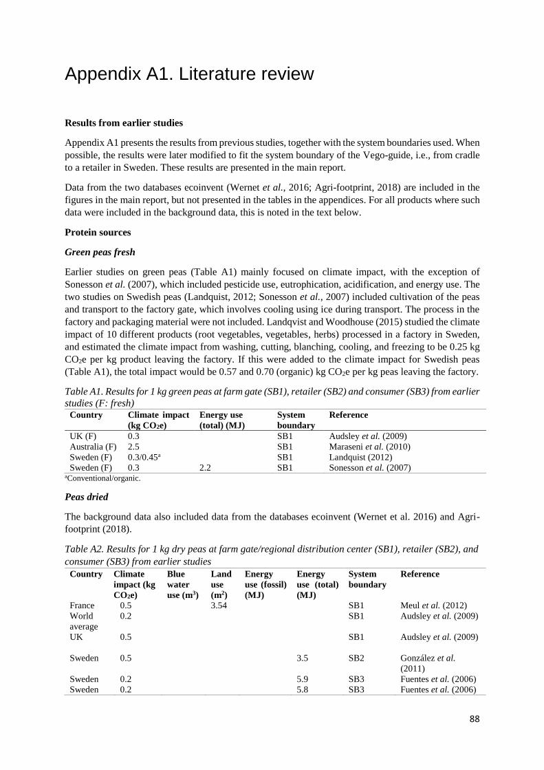
88

Appendix A1. Literature review

Results from earlier studies

Appendix A1 presents the results from previous studies, together with the system boundaries used. When

possible, the results were later modified to fit the system boundary of the Vego-guide, i.e., from cradle

to a retailer in Sweden. These results are presented in the main report.

Data from the two databases ecoinvent (Wernet et al., 2016; Agri-footprint, 2018) are included in the

figures in the main report, but not presented in the tables in the appendices. For all products where such

data were included in the background data, this is noted in the text below.

Protein sources

Green peas fresh

Earlier studies on green peas (Table A1) mainly focused on climate impact, with the exception of

Sonesson et al. (2007), which included pesticide use, eutrophication, acidification, and energy use. The

two studies on Swedish peas (Landquist, 2012; Sonesson et al., 2007) included cultivation of the peas

and transport to the factory gate, which involves cooling using ice during transport. The process in the

factory and packaging material were not included. Landqvist and Woodhouse (2015) studied the climate

impact of 10 different products (root vegetables, vegetables, herbs) processed in a factory in Sweden,

and estimated the climate impact from washing, cutting, blanching, cooling, and freezing to be 0.25 kg

CO2e per kg product leaving the factory. If this were added to the climate impact for Swedish peas

(Table A1), the total impact would be 0.57 and 0.70 (organic) kg CO2e per kg peas leaving the factory.

Table A1. Results for 1 kg green peas at farm gate (SB1), retailer (SB2) and consumer (SB3) from earlier

studies (F: fresh) Country Climate impact

(kg CO2e)

Energy use

(total) (MJ)

System

boundary

Reference

UK (F) 0.3 SB1 Audsley et al. (2009)

Australia (F) 2.5 SB1 Maraseni et al. (2010)

Sweden (F) 0.3/0.45a SB1 Landquist (2012)

Sweden (F) 0.3 2.2 SB1 Sonesson et al. (2007) aConventional/organic.

Peas dried

The background data also included data from the databases ecoinvent (Wernet et al. 2016) and Agri-

footprint (2018).

Table A2. Results for 1 kg dry peas at farm gate/regional distribution center (SB1), retailer (SB2), and

consumer (SB3) from earlier studies

Country Climate

impact (kg

CO2e)

Blue

water

use (m3)

Land

use

(m2)

Energy

use (fossil)

(MJ)

Energy

use (total)

(MJ)

System

boundary

Reference

France 0.5 3.54 SB1 Meul et al. (2012)

World

average

0.2 SB1 Audsley et al. (2009)

UK 0.5 SB1 Audsley et al. (2009)

Sweden 0.5 3.5 SB2 González et al.

(2011)

Sweden 0.2 5.9 SB3 Fuentes et al. (2006)

Sweden 0.2 5.8 SB3 Fuentes et al. (2006)

89

Sweden 0.2 SB1 Tidåker et al. (2020)

Manuscript

Sweden 0.2 SB1 Tidåker et al. (2020)

(organic) Manuscript

Sweden 0.6 2.5 SB2 Moberg et al. (2020)

Beans dried

The background data also included data from the database Agri-footprint (2018).

All studies on dry beans showed a lower climate impact than 1 kg CO2e per kg (Table A3), with the

exception of Agri-footprint (2018) data for Dutch beans, which was primarily due to higher nitrogen

fertilizer application, with related dinitrogen monoxide emissions.

Table A3. Results for 1 kg dry beans at farm gate/regional distribution center (SB1), retailer (SB2),

and consumer (SB3) from earlier studies

Country/region Climate

impact (kg

CO2e)

Land

use

(m2)

Energy

use (fossil)

(MJ)

Energy

use (total)

(MJ)

System

boundary

Reference

Greece 0.3 SB1 Abeliotis et al.

(2013)

Greece 0.4 SB1 Abeliotis et al.

(2013)

Greece 0.4 SB1 Abeliotis et al.

(2013) (organic)

USA 0.7 10 SB3 Fuentes et al. (2006)

Greece 0.2 3.7 SB1 Abeliotis et al.

(2013)

Greece 0.3 3.57 SB1 Abeliotis et al.

(2013)

Greece 0.4 3.19 SB1 Abeliotis et al.

(2013) (organic)

The Netherlands 0.6 7.9 SB3 Fuentes et al. (2006)

EU 0.6 SB1 Audsley et al. (2009)

Sweden 0.7 7.4 SB2 González et al.

(2011)

Sweden 0.3 7.25 SB3 Fuentes et al. (2006)

Sweden 0.4 7.50 SB3 Fuentes et al. (2006)

Sweden 0.4 SB1 Tidåker et al. (2020)

manuscript

Sweden 0.8 7.6 SB2 Moberg et al. (2020)

Faba beans dried

The background data also included data from the databases ecoinvent (Wernet et al., 2016) and Agri-

footprint (2018).

Table A4. Results for 1 kg dry faba beans at farm gate/regional distribution center (SB1), retailer (SB2),

and consumer (SB3) from earlier studies

Country Climate impact

(kg CO2e)

Land

use

(m2)

Energy

use

(fossil)

(MJ)

Energy use

(total) (MJ)

System

boundary

Reference

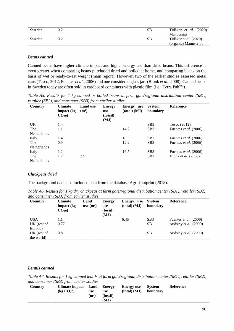
90

Sweden 0.2 SB1 Tidåker et al. (2020)

Manuscript

Sweden 0.2 SB1 Tidåker et al. (2020)

(organic) Manuscript

Beans canned

Canned beans have higher climate impact and higher energy use than dried beans. This difference is

even greater when comparing beans purchased dried and boiled at home, and comparing beans on the

basis of wet or ready-to-eat weight (main report). However, two of the earlier studies assessed metal

cans (Tesco, 2012; Fuentes et al., 2006) and one considered glass jars (Blonk et al., 2008). Canned beans

in Sweden today are often sold in cardboard containers with plastic film (i.e., Tetra Pak™).

Table A5. Results for 1 kg canned or boiled beans at farm gate/regional distribution center (SB1),

retailer (SB2), and consumer (SB3) from earlier studies

Country Climate

impact (kg

CO2e)

Land use

(m2)

Energy

use

(fossil)

(MJ)

Energy use

(total) (MJ)

System

boundary

Reference

UK 1.4 SB3 Tesco (2012)

The

Netherlands

1.1 14.2 SB3 Fuentes et al. (2006)

Italy 1.4 18.5 SB3 Fuentes et al. (2006)

The

Netherlands

0.9 12.2 SB3 Fuentes et al. (2006)

Italy 1.2 16.5 SB3 Fuentes et al. (2006)

The

Netherlands

1.7 3.5 SB2 Blonk et al. (2008)

Chickpeas dried

The background data also included data from the database Agri-footprint (2018).

Table A6. Results for 1 kg dry chickpeas at farm gate/regional distribution center (SB1), retailer (SB2),

and consumer (SB3) from earlier studies Country Climate

impact (kg

CO2e)

Land

use (m2)

Energy

use

(fossil)

(MJ)

Energy use

(total) (MJ)

System

boundary

Reference

USA 1.1 6.45 SB3 Fuentes et al. (2006)

UK (rest of

Europe)

0.77 SB1 Audsley et al. (2009)

UK (rest of

the world)

0.8 SB1 Audsley et al. (2009)

Lentils canned

Table A7. Results for 1 kg canned lentils at farm gate/regional distribution center (SB1), retailer (SB2),

and consumer (SB3) from earlier studies

Country Climate impact

(kg CO2e)

Land

use

(m2)

Energy

use

(fossil)

(MJ)

Energy use

(total) (MJ)

System

boundary

Reference

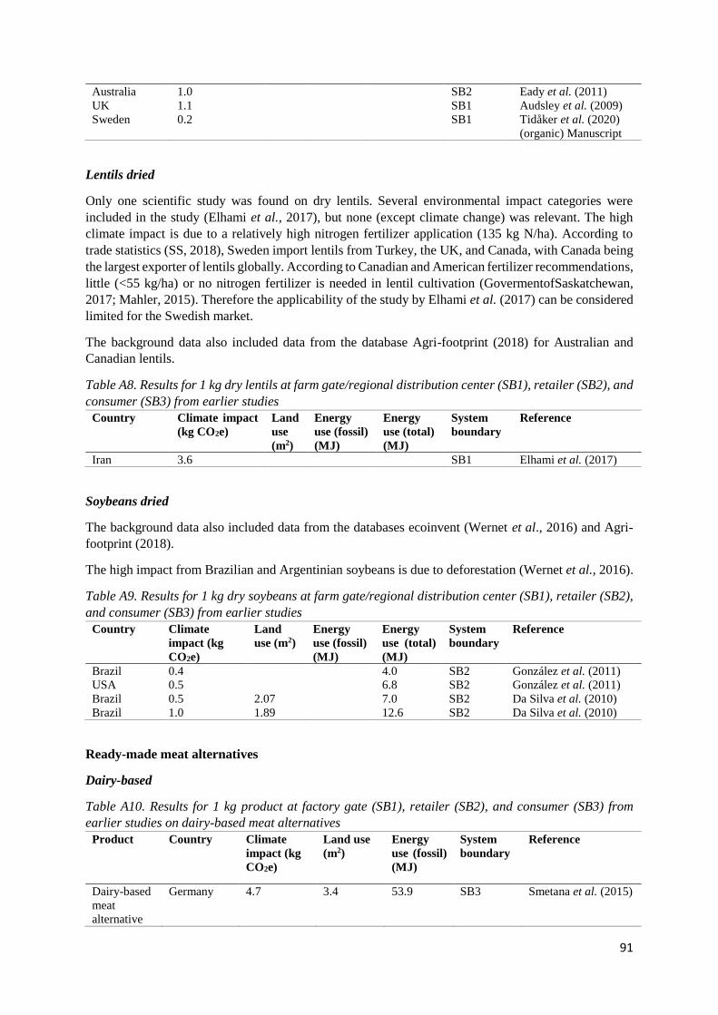
91

Australia 1.0 SB2 Eady et al. (2011)

UK 1.1 SB1 Audsley et al. (2009)

Sweden 0.2 SB1 Tidåker et al. (2020)

(organic) Manuscript

Lentils dried

Only one scientific study was found on dry lentils. Several environmental impact categories were

included in the study (Elhami et al., 2017), but none (except climate change) was relevant. The high

climate impact is due to a relatively high nitrogen fertilizer application (135 kg N/ha). According to

trade statistics (SS, 2018), Sweden import lentils from Turkey, the UK, and Canada, with Canada being

the largest exporter of lentils globally. According to Canadian and American fertilizer recommendations,

little (<55 kg/ha) or no nitrogen fertilizer is needed in lentil cultivation (GovermentofSaskatchewan,

2017; Mahler, 2015). Therefore the applicability of the study by Elhami et al. (2017) can be considered

limited for the Swedish market.

The background data also included data from the database Agri-footprint (2018) for Australian and

Canadian lentils.

Table A8. Results for 1 kg dry lentils at farm gate/regional distribution center (SB1), retailer (SB2), and

consumer (SB3) from earlier studies

Country Climate impact

(kg CO2e)

Land

use

(m2)

Energy

use (fossil)

(MJ)

Energy

use (total)

(MJ)

System

boundary

Reference

Iran 3.6 SB1 Elhami et al. (2017)

Soybeans dried

The background data also included data from the databases ecoinvent (Wernet et al., 2016) and Agri-

footprint (2018).

The high impact from Brazilian and Argentinian soybeans is due to deforestation (Wernet et al., 2016).

Table A9. Results for 1 kg dry soybeans at farm gate/regional distribution center (SB1), retailer (SB2),

and consumer (SB3) from earlier studies

Country Climate

impact (kg

CO2e)

Land

use (m2)

Energy

use (fossil)

(MJ)

Energy

use (total)

(MJ)

System

boundary

Reference

Brazil 0.4 4.0 SB2 González et al. (2011)

USA 0.5 6.8 SB2 González et al. (2011)

Brazil 0.5 2.07 7.0 SB2 Da Silva et al. (2010)

Brazil 1.0 1.89 12.6 SB2 Da Silva et al. (2010)

Ready-made meat alternatives

Dairy-based

Table A10. Results for 1 kg product at factory gate (SB1), retailer (SB2), and consumer (SB3) from

earlier studies on dairy-based meat alternatives

Product Country Climate

impact (kg

CO2e)

Land use

(m2)

Energy

use (fossil)

(MJ)

System

boundary

Reference

Dairy-based

meat

alternative

Germany 4.7 3.4 53.9 SB3 Smetana et al. (2015)

92

Milk protein The

Netherlands

5.6 4.4 36.0 SB2 Broekema and Blonk

(2009)

Mixed (bean burgers and falafel)

This category contains a wide variety of products, including falafel, schnitzel, and bean burgers. All

results from the study by Quantis (2016) include cooking in the USA, and this had a rather high impact

on the results. With cooking and transport home, the climate impact was found to be 5.8 kg CO2e per

kg, while the same product had an impact of 3.1 kg CO2e per kg up to the retailer (Quantis, 2016).

Table A11. Results for 1 kg product at factory gate (SB1), retailer (SB2), and consumer (SB3) from

earlier studies on mixed products (bean burgers and falafel) (F: fresh, FZ: frozen)

Product Country Climate

impact

(kg

CO2e)

Blue

water

use

(m3)

Land use

(m2)

Energy

use (fossil)

(MJ)

System

boundary

Reference

Schnitzel (F) The

Netherlands

2.2 4.5 25 SB2 Broekema and

Blonk (2009)

“Meatballs”

(F)

The

Netherlands

2.1 3.6 25 SB2 Broekema and

Blonk (2009)

Chick-pea

patties (FZ)

USA 5.8 0.04 SB3 Quantis (2016)

Falafel (FZ) The

Netherlands

2.5 2.5 SB2 Head et al. (2011)

Burger The

Netherlands

3.5 0.05 5.2 SB3 Consultants (2017)

Burger The

Netherlands

3.0 0.05 4 SB3 Consultants (2017)

Falafel (FZ) Sweden 0.7 SB1 Orklafoods (L.

Lundahl, 2018)

Mixed with eggs (or cheese)

Some vegetarian products include eggs or other products of animal origin. It is interesting to note that

Dutch and Swedish products seem to have a climate impact in the same range (1.5-2.5 kg CO2e per kg

product). Again, the products from the study by Quantis (2016) show a high impact, and cooking is a

substantial part of this, with impact including cooking (excluding cooking) of: 9.2 (6.9), 6.9 (5.8), and

11.3 (6.9) kg CO2e per kg product. Impact up to retailer (i.e., excluding cooking) is still substantially

higher for these products. They generally have long ingredients lists containing wheat protein, soy

protein, etc. (Quantis, 2016).

Table A12. Results for 1 kg product at factory gate (SB1), retailer (SB2), and consumer (SB3) from

earlier studies on mixed with eggs (F: fresh, FZ: frozen)

Product Country Climate

impact

(kg

CO2e)

Blue

water

use

(m3)

Land

use

(m2)

Energy

use

(fossil)

(MJ)

Energy

use

(total)

(MJ)

System

boundary

Reference

93

Sausage (F) The

Netherlands

1.5 2.8 24 SB2 Broekema and

Blonk (2009)

Burger (F) The

Netherlands

2.1 2.5 22.5 SB2 Broekema and

Blonk (2009)

Grilled

pieces (F)

The

Netherlands

2.2 3.4 27 SB2 Broekema and

Blonk (2009)

“Meatballs”

(F)

The

Netherlands

2.5 2.4 22.5 SB2 Broekema and

Blonk (2009)

Bean burger

(FZ)

USA 9.2 0.04 SB3 Quantis (2016)

Bean burger

(FZ)

USA 6.9 0.03 SB3 Quantis (2016)

Sausage

patties (FZ)

USA 11.3 0.04 SB3 Quantis (2016)

“Carrotballs

” (FZ)

Sweden 2.0 SB1 Orklafoods (L.

Lundahl, 2018)

Burger (FZ) Sweden 1.7 SB1 Orklafoods (L.

Lundahl, 2018)

Pea-protein

Table A13. Results for 1 kg product at factory gate (SB1), retailer (SB2), and consumer (SB3) from

earlier studies on pea protein based products (F: fresh, FZ: frozen)

Product Country Climate

impact (kg

CO2e)

Land use

(m2)

Energy

use (total)

(MJ)

System

boundary

Reference

Pea protein

(FZ)

Sweden 3.1 4.9 57 SB2 Nilsson and Florén

(2017)

Quorn - Mycoprotein

Results for mycoprotein (generally known as Quorn) seem to vary greatly. One reason could be that the

process for growing mycoprotein is quite energy-demanding, so the energy source will be important.

Two studies show higher impact than the others (Smetana et al., 2015; Finnigan et al., 2010). The latter

study was later updated to report significantly lower impact (Finnigan et al., 2017). Smetana et al. (2015)

included cooking, which accounted for approximately 25% of the impact. Energy use in the process of

producing mycoprotein was another important contributor. Smetana et al. (2015) only report weighted

results for process contribution, and information on the importance of cooking for climate impact and

energy used could therefore not be retrieved.

Table A14. Results for 1 kg product at factory gate (SB1), retailer (SB2), and consumer (SB3) from

earlier studies on Quorn (assumption that all is frozen)

Product Country Climate

impact

(kg

CO2e)

Blue

water

use

(m3)

Land

use

(m2)

Energy

use

(fossil)

(MJ)

Energy

use

(total)

(MJ)

System

boundary

Reference

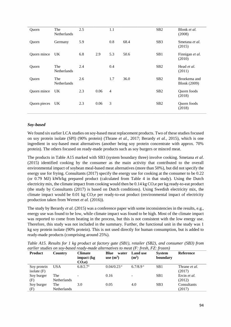
94

Quorn The

Netherlands

2.5 1.1 SB2 Blonk et al.

(2008)

Quorn Germany 5.9 0.8 68.4 SB3 Smetana et al.

(2015)

Quorn mince UK 6.8 2.9 5.3 50.6 SB1 Finnigan et al.

(2010)

Quorn The

Netherlands

2.4 0.4 SB2 Head et al.

(2011)

Quorn The

Netherlands

2.6 1.7 36.0 SB2 Broekema and

Blonk (2009)

Quorn mince UK 2.3 0.06 4 SB2 Quorn foods

(2018)

Quorn pieces UK 2.3 0.06 3 SB2 Quorn foods

(2018)

Soy-based

We found six earlier LCA studies on soy-based meat replacement products. Two of these studies focused

on soy protein isolate (SPI) (90% protein) (Thrane et al., 2017; Berardy et al., 2015), which is one

ingredient in soy-based meat alternatives (another being soy protein concentrate with approx. 70%

protein). The others focused on ready-made products such as soy burgers or minced meat.

The products in Table A15 marked with SB3 (system boundary three) involve cooking. Smetana et al.

(2015) identified cooking by the consumer as the main activity that contributed to the overall

environmental impact of soybean meal-based meat alternatives (more than 50%), but did not specify the

energy use for frying. Consultants (2017) specify the energy use for cooking at the consumer to be 0.22

(or 0.79 MJ) kWh/kg prepared product (calculated from Table 4 in that study). Using the Dutch

electricity mix, the climate impact from cooking would then be 0.14 kg CO2e per kg ready-to-eat product

(the study by Consultants (2017) is based on Dutch conditions). Using Swedish electricity mix, the

climate impact would be 0.01 kg CO2e per ready-to-eat product (environmental impact of electricity

production taken from Wernet et al. (2016)).

The study by Berardy et al. (2015) was a conference paper with some inconsistencies in the results, e.g.,

energy use was found to be low, while climate impact was found to be high. Most of the climate impact

was reported to come from heating in the process, but this is not consistent with the low energy use.

Therefore, this study was not included in the summary. Further, the functional unit in the study was 1

kg soy protein isolate (90% protein). This is not used directly for human consumption, but is added to

ready-made products (comprising around 25%).

Table A15. Results for 1 kg product at factory gate (SB1), retailer (SB2), and consumer (SB3) from

earlier studies on soy-based ready-made alternatives to meat (F: fresh, FZ: frozen)

Product Country Climate

impact (kg

CO2e)

Blue water

use (m3)

Land use

(m2)

System

boundary

Reference

Soy protein

isolate (F)

USA 6.8/2.7a 0.04/0.23 a 6.7/8.9 a SB1 Thrane et al.

(2017)

Soy burger

(F)

The

Netherlands

- 0.16 - SB1 Ercin et al.

(2012)

Soy burger

(F)

The

Netherlands

3.0 0.05 4.0 SB3 Consultants

(2017)

95

Soy meal

based (F)

Germany

2.7 - 1.3 SB3 Smetana et al.

(2015)

Soy minced

meat 1

(frozen) (F)

The

Netherlands

2.2 0.05 3.0 SB3 Consultants

(2017)

Soy minced

meat 2

(frozen) (F)

The

Netherlands

2.7 0.06 4.9 SB3 Consultants

(2017)

Soy minced

meat (FZ)

USA 6.0 (2.7) 0.03 (0.02) - SB3 (SB1) Quantis (2016)

Soy burger

(FZ)

USA 7.4 (4.6) 0.02 (0.01) - SB3 (SB1) Quantis (2016)

Soy burger

(FZ)

The

Netherlands

3.5 0.06 4 SB3 Consultants

(2017)

Soy

“chicken

pieces” 1

(FZ)

The

Netherlands

1.5 0.03 8 SB3 Consultants

(2017)

Soy

“chicken

pieces” 2

(FZ)

The

Netherlands

2.5 0.06 4.2 SB3 Consultants

(2017)

Soy-based

products

(FZ)

Sweden 1.4-2.2

(average: 1.6)b

Orklafoods (L.

Lundahl, 2018)

aAttributional/consequential modelling. bEleven different soy-based products.

Tofu and tempeh

The background data also included data from the database ecoinvent (Wernet et al., 2016).

Table A16. Results for 1 kg product at factory gate (SB1), retailer (SB2), and consumer (SB3) from

earlier studies on tofu and tempeh Product Country Climate

impact (kg

CO2e)

Blue

water

use

(m3)

Land

use

(m2)

Energy

use

(fossil)

(MJ)

Energy

use

(total)

(MJ)

System

boundary

Reference

Tofu USA 1.0 SB1 Mejia et al.

(2018)

Tofu The

Netherlands

2.0 2.0 27.5 SB2 Broekema and

Blonk (2009)

Tofu The

Netherlands

2.2 2.8 28.0 SB2 Broekema and

Blonk (2009)

Tofu The

Netherlands

3.1 2.16 SB2 Head et al.

(2011)

Tofu The

Netherlands

2.3 3.5 SB2 Blonk et al.

(2008)

Tempeh The

Netherlands

1.3 2 SB2 Blonk et al.

(2008)

Nuts and seeds

Almonds

96

The majority of global almond production is in California, USA. Most of the earlier studies identified

in this assessment estimated the climate impact for American almonds, and all found values below 4 kg

CO2e per kg (Kendall et al., 2015; Kendall & Brodt, 2014; Marvinney et al., 2014; Venkat, 2012).

Bartzas et al. (2017) estimated the climate impact to be approximately 2 kg CO2e per kg for Greek

almonds in shell, with irrigation (pumping groundwater) and fertilizer production having the greatest

impact on the result. In that assessment (Bartzas et al., 2017), it was assumed that about 1.7 kg almonds

in shell are required for 1 kg shelled almonds, which results in an impact of 3.4 kgCO2e per kg almonds.

The data in Volpe et al. (2015) for primary production were based on Marvinney et al. (2014), and

therefore Volpe et al. (2015) was excluded from the recommendation.

The background data also included data from the database ecoinvent (Wernet et al., 2016).

Table A17. Results for 1 kg almonds at farm gate (SB1), retailer (SB2), and consumer (SB3) from earlier

studies

Country Climate

impact

(kg

CO2e)

Blue

water

use

(m3)

Total

water

use

(m3)

Land

use

(m2)

Energy

use

(fossil)

(MJ)

Energy

use

(total)

(MJ)

System

boundary

Reference

USA 0.5 SB1 Kendall and Brodt

(2014)

World 1.2 SB1 Nemecek et al.

(2012)

USA 1.9 12.9 SB1 Marvinney et al.

(2014)

USA 2.5/3.8a SB1 Venkat (2012)

Greece 3.4b 2.4 47.7 SB1 Bartzas et al. (2017)

USA 0.9/1.5c 29/33c SB1 Kendall et al. (2015)

USA

(California)

539 10.2 SB1 Fulton et al. (2018)

Italy 1.9 SB1 Volpe et al. (2015)

Rest of

world

0.9 SB1 Audsley et al. (2009)

aConventional/organic. bAssuming that about 1.7 kg almonds in shells are required for 1 kg almonds. cSystem expansion/economic allocation.

Cashew nuts

Table A18. Results for 1 kg cashew nuts at farm gate (SB1), retailer (SB2), and consumer (SB3) from

earlier studies

Country Climate

impact

(kg

CO2e)

Total

water

use

(m3)

Land

use

(m2)

Energy

use

(fossil)

(MJ)

Energy

use (total)

(MJ)

System

boundary

Reference

Rest of

Europe

1.2 SB1 Audsley et al. (2009)

Brazil 1.4/1.5a SB1 de Figueirêdo et al.

(2014)

Netherlands 2.3 18.0 SB2 Blonk et al. (2008) aTraditional practice/observed field notes.

Chestnuts

97

Table A19. Results for 1 kg chestnuts at farm gate (SB1), retailer (SB2), and consumer (SB3) from

earlier studies

Country Climate

impact (kg

CO2e)

Total

water

use (m3)

Land

use

(m2)

Energy

use (fossil)

(MJ)

Energy

use (total)

(MJ)

System

boundary

Reference

Rest of

Europe

0.4 SB1 Audsley et al.

(2009)

Portugal 0.9/0.4a 11.0/4.0 SB1 Rosa et al. (2017) aTwo different producers: producer 1/producer 2.

Coconuts

Only one earlier study was found on coconuts (Audsley et al., 2009), which focused solely on climate

impact. The results included transportation to a regional distribution center in the UK from rest of the

world. The background data also included data from the database Agri-footprint (2018).

Table A20. Results for 1 kg coconuts at farm gate (SB1), retailer (SB2), and consumer (SB3) from earlier

studies

Country Climate

impact (kg

CO2e)

Blue

water

use (m3)

Land

use

(m2)

Energy

use

(fossil)

(MJ)

Energy

use

(total)

(MJ)

System

boundary

Reference

Rest of the worlda 1.8 SB1 Audsley et al.

(2009) aIncluding copra (coconut flesh).

Groundnuts/peanuts

The background data also included data from the databases ecoinvent (Wernet et al., 2016) and Agri-

footprint (2018).

Table A21. Results for 1 kg groundnuts/peanuts at farm gate (SB1), retailer (SB2), and consumer (SB3)

from earlier studies

Country Climate

impact

(kg

CO2e)

Total

water

use

(m3)

Land

use

(m2)

Energy

use (fossil)

(MJ)

Energy

use (total)

(MJ)

System

boundary

Reference

Netherlands 1.5 3.90 SB2 Blonk et al. (2008)

USA 0.8a SB1 Mccarty et al. (2012)

USA 1.7b SB2 Mccarty et al. (2012)

UK 0.9 SB1 Audsley et al. (2009)

USA 1.1 SB1 Nemecek et al. (2012) aIncluding four different irrigation scenarios. bPeanut butter.

Hazelnuts

Table A22. Results for 1 kg hazelnuts at farm gate (SB1), retailer (SB2), and consumer (SB3) from

earlier studies

Country Climate

impact

(kg

CO2e)

Total

water

use

(m3)

Land

use

(m2)

Energy

use (fossil)

(MJ)

Energy

use (total)

(MJ)

System

boundary

Reference

98

Rest of

Europe

0.4 SB1 Audsley et al. (2009)

World 1.5 SB1 Nemecek et al. (2012)

Italy 0.5 SB1 Volpe et al. (2015)

Walnuts

In some of the identified studies, the walnuts were assumed to be shelled (Venkat, 2012; Audsley et al.,

2010; Blonk et al., 2008). In the main report, data for all nuts were recalculated to show the results for

shelled product.

Table A23. Results for 1 kg walnuts at farm gate (SB1), retailer (SB2), and consumer (SB3) from earlier

studies

Country Climate

impact

(kg

CO2e)

Blue

water

use

(m3)

Total

water

use

(m3)

Land

use

(m2)

Energy

use

(fossil)

(MJ)

Energy

use

(total)

(MJ)

System

boundary

Reference

Netherlands 2.1 4.0 SB2 Blonk et al. (2008)

USA

(organic)

2.9 SB1 Venkat (2012)

Rest of

world

0.9 SB1 Audsley et al. (2009)

USA 0.9 3.9 SB1 Marvinney et al.

(2014)

Pistachios

Looking at the results for shelled nuts, Bartzas et al. (2017) had the highest impact (main report).

Assuming that 2.01 kg pistachios in shell are required for 1 kg shelled pistachios (Marvinney et al.,

2014), climate impact for the Bartzas et al. (2017) assessment would be 4.3 kg CO2e per kg pistachios.

This is much higher than in the other studies (Table A24). Using the functional unit “1 kg nuts in shell”

as in Bartzas et al. (2017), none of the impact is allocated to the shells (which can potentially be used as

e.g., an energy source). Another factor that could explain the higher impact in Bartzas et al. (2017) is

that the yield was much lower than for Marvinney et al. (2014). The data in Volpe et al. (2015) for

primary production were based on Marvinney et al. (2014), and therefore Volpe et al. (2015) was

excluded from the recommendation.

Table A24. Results for 1 kg pistachios at farm gate (SB1), retailer (SB2), and consumer (SB3) from

earlier studies

Country Climate

impact

(kg

CO2e)

Blue

water

use

(m3)

Total

water

use

(m3)

Land

use

(m2)

Energy

use

(fossil)

(MJ)

Energy

use

(total)

(MJ)

System

boundary

Reference

UK 0.9 SB1 Audsley et al. (2009)

USA 2.2 3.8 SB1 Marvinney et al.

(2014)

Greecea 2.1 1.8 27 SB1 Bartzas et al. (2017)

Italy 1.74 SB1 Volpe et al. (2015) aNuts in shell.

Linseeds

The background data were based on data from Agri-footprint (2018).

Sesame seeds

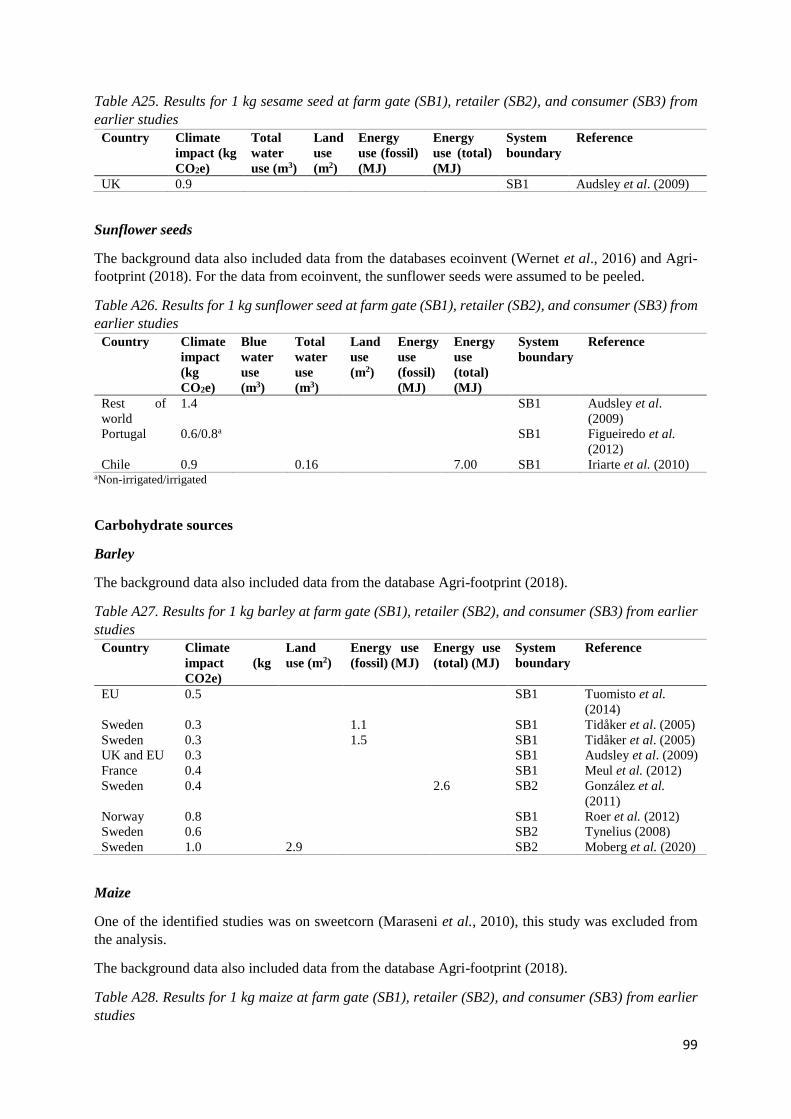
99

Table A25. Results for 1 kg sesame seed at farm gate (SB1), retailer (SB2), and consumer (SB3) from

earlier studies

Country Climate

impact (kg

CO2e)

Total

water

use (m3)

Land

use

(m2)

Energy

use (fossil)

(MJ)

Energy

use (total)

(MJ)

System

boundary

Reference

UK 0.9 SB1 Audsley et al. (2009)

Sunflower seeds

The background data also included data from the databases ecoinvent (Wernet et al., 2016) and Agri-

footprint (2018). For the data from ecoinvent, the sunflower seeds were assumed to be peeled.

Table A26. Results for 1 kg sunflower seed at farm gate (SB1), retailer (SB2), and consumer (SB3) from

earlier studies

Country Climate

impact

(kg

CO2e)

Blue

water

use

(m3)

Total

water

use

(m3)

Land

use

(m2)

Energy

use

(fossil)

(MJ)

Energy

use

(total)

(MJ)

System

boundary

Reference

Rest of

world

1.4 SB1 Audsley et al.

(2009)

Portugal 0.6/0.8a SB1 Figueiredo et al.

(2012)

Chile 0.9 0.16 7.00 SB1 Iriarte et al. (2010) aNon-irrigated/irrigated

Carbohydrate sources

Barley

The background data also included data from the database Agri-footprint (2018).

Table A27. Results for 1 kg barley at farm gate (SB1), retailer (SB2), and consumer (SB3) from earlier

studies

Country Climate

impact (kg

CO2e)

Land

use (m2)

Energy use

(fossil) (MJ)

Energy use

(total) (MJ)

System

boundary

Reference

EU 0.5

SB1 Tuomisto et al.

(2014)

Sweden 0.3 1.1 SB1 Tidåker et al. (2005)

Sweden 0.3 1.5 SB1 Tidåker et al. (2005)

UK and EU 0.3 SB1 Audsley et al. (2009)

France 0.4 SB1 Meul et al. (2012)

Sweden 0.4 2.6 SB2 González et al.

(2011)

Norway 0.8 SB1 Roer et al. (2012)

Sweden 0.6 SB2 Tynelius (2008)

Sweden 1.0 2.9 SB2 Moberg et al. (2020)

Maize

One of the identified studies was on sweetcorn (Maraseni et al., 2010), this study was excluded from

the analysis.

The background data also included data from the database Agri-footprint (2018).

Table A28. Results for 1 kg maize at farm gate (SB1), retailer (SB2), and consumer (SB3) from earlier

studies

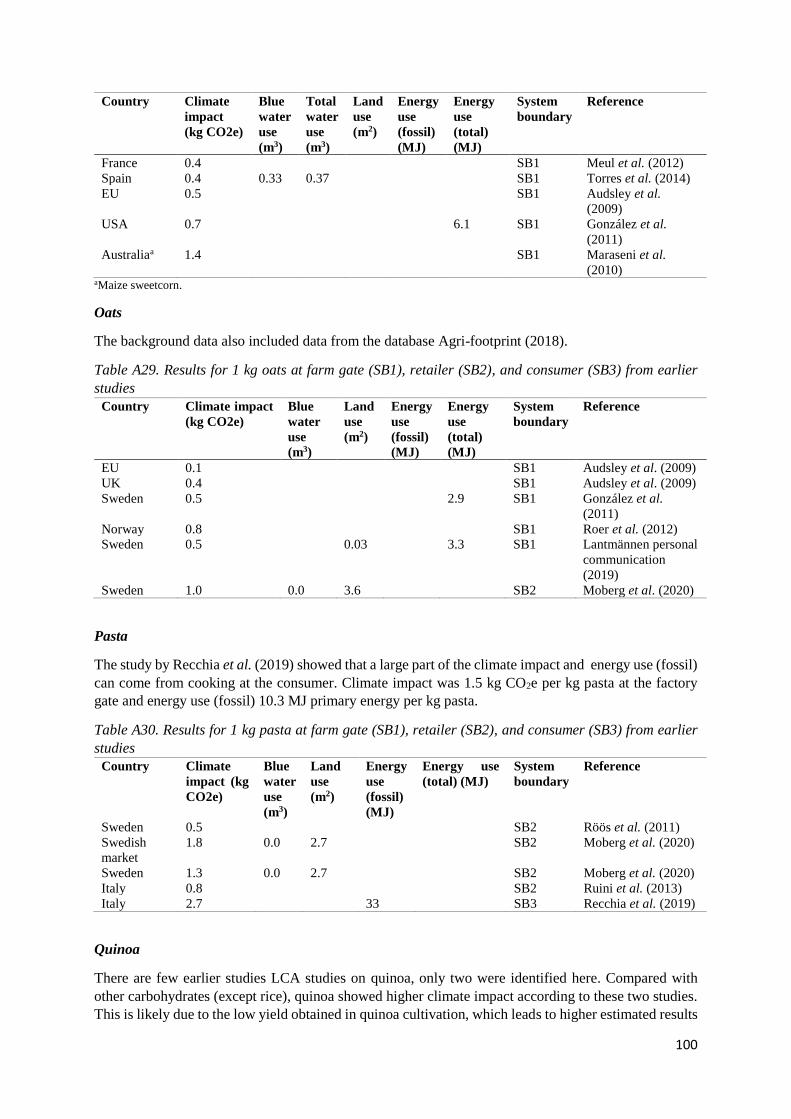
100

Country Climate

impact

(kg CO2e)

Blue

water

use

(m3)

Total

water

use

(m3)

Land

use

(m2)

Energy

use

(fossil)

(MJ)

Energy

use

(total)

(MJ)

System

boundary

Reference

France 0.4 SB1 Meul et al. (2012)

Spain 0.4 0.33 0.37 SB1 Torres et al. (2014)

EU 0.5 SB1 Audsley et al.

(2009)

USA 0.7 6.1 SB1 González et al.

(2011)

Australiaa 1.4 SB1 Maraseni et al.

(2010) aMaize sweetcorn.

Oats

The background data also included data from the database Agri-footprint (2018).

Table A29. Results for 1 kg oats at farm gate (SB1), retailer (SB2), and consumer (SB3) from earlier

studies

Country Climate impact

(kg CO2e)

Blue

water

use

(m3)

Land

use

(m2)

Energy

use

(fossil)

(MJ)

Energy

use

(total)

(MJ)

System

boundary

Reference

EU 0.1 SB1 Audsley et al. (2009)

UK 0.4 SB1 Audsley et al. (2009)

Sweden 0.5 2.9 SB1 González et al.

(2011)

Norway 0.8 SB1 Roer et al. (2012)

Sweden 0.5 0.03 3.3 SB1 Lantmännen personal

communication

(2019)

Sweden 1.0 0.0 3.6 SB2 Moberg et al. (2020)

Pasta

The study by Recchia et al. (2019) showed that a large part of the climate impact and energy use (fossil)

can come from cooking at the consumer. Climate impact was 1.5 kg CO2e per kg pasta at the factory

gate and energy use (fossil) 10.3 MJ primary energy per kg pasta.

Table A30. Results for 1 kg pasta at farm gate (SB1), retailer (SB2), and consumer (SB3) from earlier

studies

Country Climate

impact (kg

CO2e)

Blue

water

use

(m3)

Land

use

(m2)

Energy

use

(fossil)

(MJ)

Energy use

(total) (MJ)

System

boundary

Reference

Sweden 0.5 SB2 Röös et al. (2011)

Swedish

market

1.8 0.0 2.7 SB2 Moberg et al. (2020)

Sweden 1.3 0.0 2.7 SB2 Moberg et al. (2020)

Italy 0.8 SB2 Ruini et al. (2013)

Italy 2.7 33 SB3 Recchia et al. (2019)

Quinoa

There are few earlier studies LCA studies on quinoa, only two were identified here. Compared with

other carbohydrates (except rice), quinoa showed higher climate impact according to these two studies.

This is likely due to the low yield obtained in quinoa cultivation, which leads to higher estimated results

101

for quinoa (Cancino-Espinoza et al., 2018). Additionally, the postharvest process where quinoa is dried

and treated contributes to greenhouse gas emissions, as does transport through mountainous areas to the

port in Lima (Cancino-Espinoza et al., 2018).

Table A31. Results for 1 kg quinoa at farm gate (SB1), retailer (SB2), and consumer (SB3) from earlier

studies

Country Climate

impact (kg

CO2e)

Blue

water

use

(m3)

Land

use

(m2)

Energy

use

(fossil)

(MJ)

Energy

use (total)

(MJ)

System

boundary

Reference

South America 0.9 SB1 Alter eco (2012)

South Americaa 2.7 SB1 Alter eco (2012)

Perub 0.9 SB1 Cancino-Espinoza et

al. (2018) aDark quinoa. bOrganic.

Rice

Earlier studies show that rice is associated with higher climate impact than other carbohydrate sources.

Field emissions (CH4 and N2O) were the largest contributor to global warming potential in several

studies where the fields were irrigated or flooded (Brodt et al., 2014; Thanawong et al., 2014; Kägi et

al., 2010; Blengini & Busto, 2009; Hokazono et al., 2009). For example, emissions of CH4 from paddy

fields made up more than half of the total emissions estimated in Hokazono et al. (2009). The study on

upland Swiss rice cultivation (Kägi et al., 2010), where flooding was not used, showed lower emissions

of CH4. Switzerland is not a significant producer of rice globally and the study is therefore considered

less relevant for the Swedish market. The system boundary in Kägi et al. (2010) is up to a Swiss retailer,

which means that the emissions from transport to Switzerland are included in the result for American

rice.

Thanawong et al. (2014) estimated the climate impact to be 3.1-5.6 kg CO2e per kg rice, depending on

whether the field was rain-fed or irrigated and if it was wet season or dry season. These values are in the

upper range of results reported for rice. This could be because the study used higher values for CH4

emissions compared with those suggested in IPCC (2006). In addition, rice yield is relatively low in

north-east Thailand, which could have contributed to the higher climate impact (Thanawong et al.,

2014). Berners-Lee et al. (2012) estimated the climate impact for several foods, but do not provide

details of the inventory, so the higher climate impact is difficult to explain.

The background data also included data from the database Agri-footprint (2018).

Table A32. Results for 1 kg rice at farm gate (SB1), retailer (SB2), and consumer (SB3) from earlier

studies

Country Climate

impact

(kg

CO2e)

Blue

water

use

(m3)

Total

water

use

(m3)

Lan

d use

(m2)

Energy

use

(fossil)

(MJ)

Energy

use

(total)

(MJ)

System

boundar

y

Reference

Japan 1.2 7.4 SB2 González et al.

(2011)

USA 1.1 6.6 SB2 González et al.

(2011)

Japan 1.3-1.6a SB1 Hokazono et al.

(2009)

USA 1.5-3.7b SB1 Brodt et al. (2014)

Switzerland 1.7 SB2 Kägi et al. (2010)

USA 2.8 SB2 Kägi et al. (2010)

USA 2.1 SB1 Loijos (2008)

102

Italyd 2.8/2.9 4.9 8.0/8.

2

14.6/

16.6

15.7/

17.8

SB2 Blengini and Busto

(2009)

Thailande 3.1-5.6 2.7-

3.3

4.2-

4.6

7.3-9.5 SB1 Thanawong et al.

(2014)

Rest of the

world

3.5 SB1 Audsley et al. (2009)

UK 5.7 SB2 Berners-Lee et al.

(2012)

Rest of the

world

3.6 0.7 4.5 Moberg et al. (2020)

aSustainable system (low value), conventional system (in between value), environmentally friendly (high value). bUsing GWP100 (low value), GWP20 (in between value), and IPCC tier 1 (high value). cConventional/organic. dLocal distribution/exported rice. eRain-fed (low value), wet-season irrigated (in between value), dry-season irrigated (high value).

Rye

The background data also included data from the database Agri-footprint (2018).

Table A33. Results for 1 kg rye at farm gate (SB1), retailer (SB2), and consumer (SB3) from earlier

studies

Country Climate

impact (kg

CO2e)

Blue

water

use

(m3)

Land

use

(m2)

Energy

use

(fossil)

(MJ)

Energy use

(total) (MJ)

System

boundary

Reference

Sweden 0.4 2.10 SB2 González et al.

(2011)

EU 0.5 SB1 Audsley et al. (2009)

UK 0.9 SB1 Audsley et al. (2009)

Sweden 0.4 SB1 Woodhouse (2017)

Sweden 0.9 2.33 Moberg et al. (2020)

Sorghum

The background data also included data from the database Agri-footprint (2018).

Table A34. Results for 1 kg sorghum at farm gate (SB1), retailer (SB2), and consumer (SB3) from earlier

studies

Country

Climate

impact (kg

CO2e)

Blue

water

use

(m3)

Land

use

(m2)

Energy

use

(fossil)

(MJ)

Energy use

(total) (MJ)

System

boundary

Reference

UK 0.9 SB1 Audsley et al. (2009)

Wheat

Most of the earlier assessments on climate impact of wheat production showed an impact below 1 kg

CO2e per kg wheat.

The background data also included data from the database Agri-footprint (2018).

103

Table A35. Results for 1 kg wheat at farm gate (SB1), retailer (SB2), and consumer (SB3) from earlier

studies Country Climate

impact (kg

CO2e)

Blue

water

use

(m3)

Land

use

(m2)

Energy

use

(fossil)

(MJ)

Energy

use (total)

(MJ)

System

boundary

Reference

Switzerland 0.6/0.7/0.6a 2.31/3.45/3

.30

SB1 Nemecek et al.

(2010)

Germany 0.6 3.49 SB1 Nemecek et al.

(2010)

USA 0.6 4.63 SB1 Nemecek et al.

(2010)

France 0.6 3.58 SB1 Nemecek et al.

(2010)

Spain 0.8 6.42 SB1 Nemecek et al.

(2010)

Italy 0.3 SB1 Knudsen et al. (2014)

Germany 0.4 SB1 Knudsen et al. (2014)

Canada 0.4 SB1 Knudsen et al. (2014)

Sweden 0.5 SB1 Knudsen et al. (2014)

USA 0.5 SB1 Knudsen et al. (2014)

Romania 0.5 SB1 Knudsen et al. (2014)

Russia 0.5 SB1 Knudsen et al. (2014)

Sweden 0.4 2.00 SB2 González et al.

(2011)

USA 0.8 8.90 SB2 González et al.

(2011)

Sweden 0.4-0.6 SB2 Röös et al. (2011)

France 0.5 1.07 SB1 Meul et al. (2012)

UK (wheat

flour)

0.5 SB2 Espinoza-Orias et al.

(2011)

UK 0.5 SB1 Audsley et al. (2009)

EU 0.6 SB1 Audsley et al. (2009)

World 0.7 SB1 Audsley et al. (2009)

UK 0.7/0.8b 0.14/0.4

1

2.40/2.00 SB1 Williams et al. (2010)

World 1.1 SB2 Michaelowa and

Dransfeld (2008)

Norway 0.7 SB1 Roer et al. (2012)

Sweden 0.4 SB1 Woodhouse (2017)

Sweden 1.1 0.0 2.26 SB2 Moberg et al. (2020) aOrganic/extensive/integrated production. bConventional/organic.

Carrots

The background data also included data from the database Agri-footprint (2018).

Table A36. Results for 1 kg carrots at farm gate (SB1), retailer (SB2), and consumer (SB3) from earlier

studies

Country Climate

impact

(kg

CO2e)

Blue

water

use

(m3)

Land use

(m2)

Energy

use

(fossil)

(MJ)

Energy

use

(total)

(MJ)

System

boundary

Reference

Sweden

(organic)

0.04 0.23 0.38 SB1 Cederberg et al.

(2005)

Sweden 0.1/0.3a 0.22/0.26 2.38/7.60 SB2 Fuentes et al. (2006)

Netherlands 0.2 0.18 4.00 SB2 Fuentes et al. (2006)

Switzerland 0.1 1.70 SB2 González et al.

(2011)

104

Sweden 0.1 0.97 SB2 González et al.

(2011)

Sweden 0.1 1.50 SB2 Röös and Karlsson

(2013)

Netherlands 0.2 2.80 SB2 Röös and Karlsson

(2013)

Italy 0.3 4.10 SB2 Röös and Karlsson

(2013)

Australia 0.2 0.21 SB1 Maraseni et al.

(2010)

Switzerland 0.5 0.42 0.09 SB2 Stoessel et al. (2012)

UK 0.4 SB1 Audsley et al. (2009)

Sweden

(small

carrot)

0.1/0.4a SB1 Landqvist and

Woodhouse (2015)

Sweden (big

carrot)

0.1/0.3a SB1 Landqvist and

Woodhouse (2015)

Sweden 0.2/0.4b SB1 Landqvist and

Woodhouse (2015)

Sweden 0.27 0.20 0.0 SB2 Moberg et al. (2020)

Swedish

market

0.3 0.21 0.0 SB2 Moberg et al. (2020)

aFresh/frozen. bParsnips fresh/frozen.

Potatoes

The background data also included data from the database Agri-footprint (2018).

Table A37. Results for 1 kg potatoes at farm gate (SB1), retailer (SB2), and consumer (SB3) from earlier

studies

Country Climate

impact

(kg

CO2e)

Blue

water

use

(m3)

Land use

(m2)

Energy

use

(fossil)

(MJ)

Energy

use

(total)

(MJ)

System

boundary

Reference

Sweden 0.1a 0.53/0.57a SB1 Cederberg et al.

(2005)

Denmark 0.1 0.80 SB2 González et al.

(2011)

Switzerland 0.1 1.50 SB2 González et al.

(2011)

Sweden 0.2 1.50 SB2 González et al.

(2011)

USA 0.4 4.30 SB2 González et al.

(2011)

Sweden 0.1-0.2 SB2 Röös et al. (2010)

World 0.1 1.72 SB1 Nemecek (2010)

Austria 0.2a SB2 Lindenthal et al.

(2010)

Switzerland 0.2 SB2 Stoessel et al. (2012)

UK 0.2a 0.02/0.06a 1.40/1.6

0a

SB1 Williams et al. (2010)

UK 0.3 SB1 Audsley et al. (2009)

Germany 0.1 SB2 Gruber et al. (2016)

UK 0.4 SB2 Berners-Lee et al.

(2012)

Sweden 0.3 0.01 0.46 SB2 Moberg et al. (2020)

Swedish

market

0.4 0.01 0.46 SB2 Moberg et al. (2020)

Koreab 0.4 SB1 So et al. (2010)

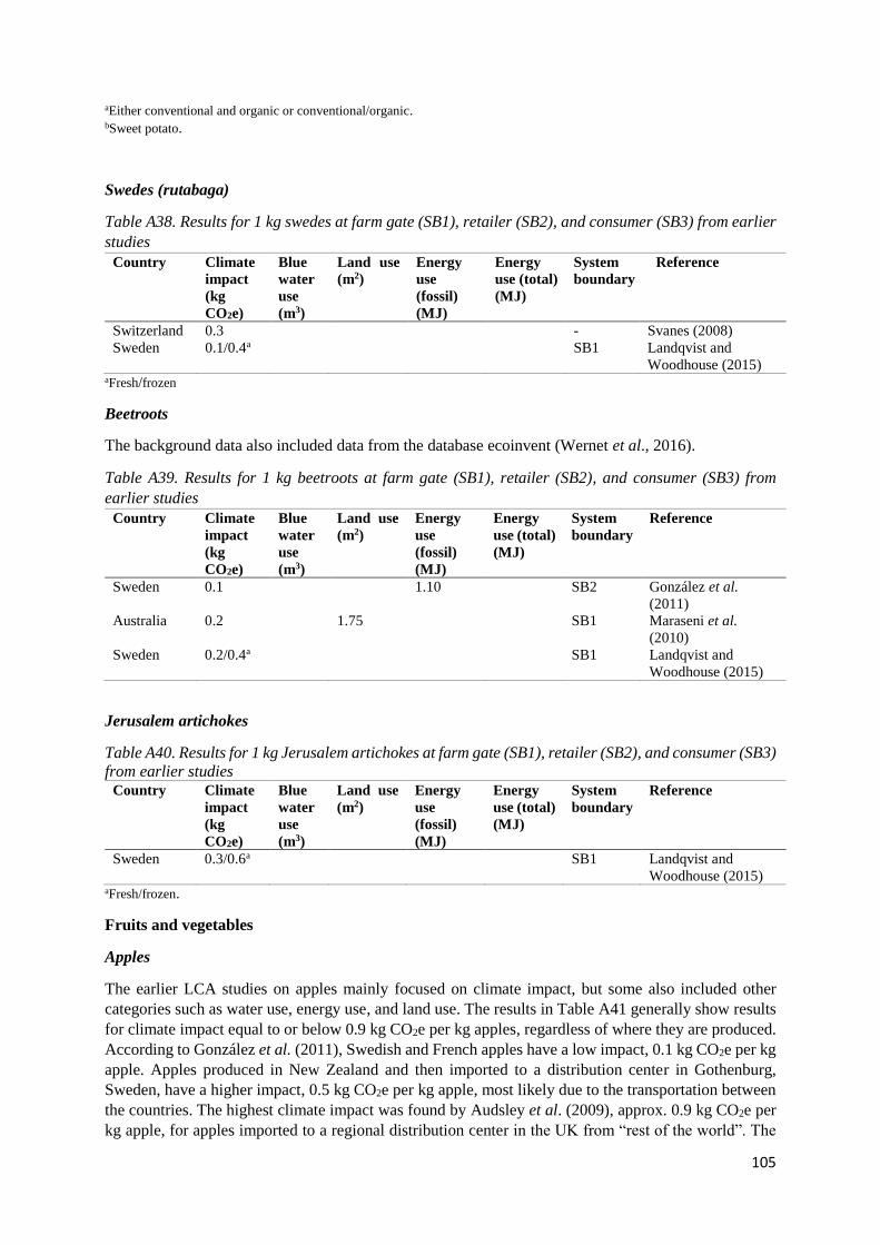
105

aEither conventional and organic or conventional/organic. bSweet potato.

Swedes (rutabaga)

Table A38. Results for 1 kg swedes at farm gate (SB1), retailer (SB2), and consumer (SB3) from earlier

studies

Country Climate

impact

(kg

CO2e)

Blue

water

use

(m3)

Land use

(m2)

Energy

use

(fossil)

(MJ)

Energy

use (total)

(MJ)

System

boundary

Reference

Switzerland 0.3 - Svanes (2008)

Sweden 0.1/0.4a SB1 Landqvist and

Woodhouse (2015) aFresh/frozen

Beetroots

The background data also included data from the database ecoinvent (Wernet et al., 2016).

Table A39. Results for 1 kg beetroots at farm gate (SB1), retailer (SB2), and consumer (SB3) from

earlier studies

Country Climate

impact

(kg

CO2e)

Blue

water

use

(m3)

Land use

(m2)

Energy

use

(fossil)

(MJ)

Energy

use (total)

(MJ)

System

boundary

Reference

Sweden 0.1 1.10 SB2 González et al.

(2011)

Australia 0.2 1.75 SB1 Maraseni et al.

(2010)

Sweden 0.2/0.4a SB1 Landqvist and

Woodhouse (2015)

Jerusalem artichokes

Table A40. Results for 1 kg Jerusalem artichokes at farm gate (SB1), retailer (SB2), and consumer (SB3)

from earlier studies Country Climate

impact

(kg

CO2e)

Blue

water

use

(m3)

Land use

(m2)

Energy

use

(fossil)

(MJ)

Energy

use (total)

(MJ)

System

boundary

Reference

Sweden 0.3/0.6a SB1 Landqvist and

Woodhouse (2015) aFresh/frozen.

Fruits and vegetables

Apples

The earlier LCA studies on apples mainly focused on climate impact, but some also included other

categories such as water use, energy use, and land use. The results in Table A41 generally show results

for climate impact equal to or below 0.9 kg CO2e per kg apples, regardless of where they are produced.

According to González et al. (2011), Swedish and French apples have a low impact, 0.1 kg CO2e per kg

apple. Apples produced in New Zealand and then imported to a distribution center in Gothenburg,

Sweden, have a higher impact, 0.5 kg CO2e per kg apple, most likely due to the transportation between

the countries. The highest climate impact was found by Audsley et al. (2009), approx. 0.9 kg CO2e per

kg apple, for apples imported to a regional distribution center in the UK from “rest of the world”. The

106

emissions that arise from transport could be a reason for the relatively high climate impact. The system

boundary in Yoshikawa et al. (2008) included stages such as production, shipping, cooking etc., but

only the stages up to retailing were accounted for here, which can be seen in Table A41. The system

boundary in Blonk et al. (2010) is up to a farm gate in the Netherlands.

According to trade statistics (SS, 2018), Sweden does not import apples from Switzerland and Peru, and

according to FAOSTAT these countries import more apples than they export. The applicability of the

studies by Stoessel et al. (2012) and Bartl et al. (2012) was therefore considered to be limited for the

Swedish market.

The background data also included data from the database ecoinvent (Wernet et al., 2016).

Table A41. Results for 1 kg apples at farm gate (SB1), retailer (SB2), and consumer (SB3) from earlier

studies

Country Climate

impact (kg

CO2e)

Blue

water

use (m3)

Land

use

(m2)

Energy use

(fossil)

(MJ)

Energy

use

(total)

(MJ)

System

boundary

Reference

New Zealand 0.04-0.1a 0.41-0.71a SB1 i Canals et al.

(2006)

New Zealand 0.1 0.95 SB1 Saunders et al.

(2006)

UK 0.3 5.0 SB1 Saunders et al.

(2006)

Italy 0.2b SB1 Cerutti et al.

(2013)

Italy 0.2 0.06 0.000

5

1.75

(calculated)

SB2 Assomela (2012)

Sweden 0.1 0.63 SB2 González et al.

(2011)

France 0.1 1.60 SB2 González et al.

(2011)

New Zealand 0.5 6.10 SB2 González et al.

(2011)

Italy 0.2 SB2 Sessa et al. (2014)

France 0.1 0.05 0.24

(calc.)

1.12 SB1 Basset-Mens et al.

(2014)

Netherlands 0.2 SB1 Blonk et al. (2010)

New Zealand 0.4 SB1 Blonk et al. (2010)

USA 0.1/0.2c SB1 Venkat (2012)

Switzerland 0.3 0.02 0.3 SB2 Stoessel et al.

(2012)

UK 0.3 SB1 Audsley et al.

(2009)

Rest of

Europe

0.4 SB1 Audsley et al.

(2009)

Rest of the

world

0.9 SB1 Audsley et al.

(2009)

USA 0.5 8.0 SB2 Renz et al. (2014)

France 0.1d 0.9-1.2d SB1 Alaphilippe et al.

(2014)

Greece 0.1 0.1 1.2 SB1 Bartzas et al.

(2017)

New Zealand 0.1 SB1 McLaren et al.

(2010)

UK 0.6 SB2 Berners-Lee et al.

(2012)

USA 0.8 SB1 Loijos (2008)

107

Japan 0.6 SB2 Yoshikawa et al.

(2008)

China 0.2 SB1 Yan et al. (2016)

Italy 0.1 1.2 SB1 Tamburini et al.

(2015)

Peru 0.4 SB1 Bartl et al. (2012)

Belgium

(conven-

tional)

0.1e SB1 Goossens et al.

(2017)

Belgium

(integrated)

0.1e SB1 Goossens et al.

(2017)

Belgium

(organic)

0.1-0.8e SB1 Goossens et al.

(2017)

Swedish

market

0.4 0.03 0.6 SB2 Moberg et al.

(2020)

Sweden 0.2 0.0 0.7 SB2 Moberg et al.

(2020) aIncluding four scenarios. bIncluding four scenarios. cConventional/organic. dIncluding two scenarios: north and south of France and extensive/semi-extensive. eIncluding young and old low productive trees and full production. Highest impact in organic orchards corresponds to young

productive trees, where the high impact is because of low yield.

Apricots

Only two earlier LCA studies were found on apricots, namely Audsley et al. (2009) and Pergola et al.

(2017). Audsley et al. (2009) showed that apricots imported from rest of Europe have a climate impact

of 0.4 kg CO2e per kg apricots. Pergola et al. (2017) showed that climate impact for three orchard

systems in Italy (including integrated and biodynamic system) ranged between 0.3-0.4 kg CO2e per kg

apricot, where the highest value corresponded to the biodynamic system. Other values for apricots and

their climate impact were taken from ecoinvent (Wernet et al., 2016), which all showed results below

0.4 kg CO2e per kg apricot.

Table A42. Results for 1 kg apricots at farm gate (SB1), retailer (SB2), and consumer (SB3) from earlier

studies

Country Climate

impact

(kg

CO2e)

Blue

water

use (m3)

Land

use

(m2)

Energy

use

(fossil)

(MJ)

Energy

use

(total)

(MJ)

System

boundary

Reference

Europe 0.4 SB1 Audsley et al.

(2009)

Italy 0.3-0.4a SB1 Pergola et al.

(2017) aThree orchard systems, including two cultivation systems: integrated (lower value) and biodynamic which is similar to

organic farming (higher value).

Bananas

Several earlier LCA studies were found on bananas, mainly focusing on the climate impact of bananas

from Ecuador, Costa Rica, Colombia, China, and Spain. All earlier studies included overseas transport

from Ecuador, Costa Rica, or Colombia to a European country or to USA, except those by Yan et al.

(2016) and Aguilera et al. (2015). The particularly high value given in Svanes and Aronsson (2013),

1.4 kg CO2e per kg banana, may be due to several reasons, e.g., the assumptions of using small ships

(i.e., higher fuel usage per unit of banana transported) and empty return. In addition, the transport

108

distance from Costa Rica to Norway, which is accounted for in Svanes and Aronsson (2013), is greater

than the distance to e.g., a German retailer.

The background data also included data from the database ecoinvent (Wernet et al., 2016).

Table A43. Results for 1 kg bananas at farm gate (SB1), retailer (SB2), and consumer (SB3) from earlier

studies

Country Climate

impact (kg

CO2e)

Blue

water

use (m3)

Land

use

(m2)

Energy

use

(fossil)

(MJ)

Energy

use

(total)

(MJ)

System

boundary

Reference

Ecuador 0.5/1.0a SB2 Iriarte et al. (2014)

Ecuador 0.5 SB1 Blonk et al. (2010)

Switzerland

(origin

Colombia)

0.5 0.08 0.2 SB2 Stoessel et al.

(2012)

USA (origin

Costa Rica)

0.5 5.5 SB2 Renz et al. (2014)

EU (imported) 0.6 SB2 Lescot (2012)

EU (imported) 0.7 SB2 Lescot (2012)

EU (imported) 0.9 SB2 Lescot (2012)

EU (imported) 1.1 SB2 Lescot (2012)

UK (origin

probably Costa

Rica or

Ecuador)

0.7 SB2 Berners-Lee et al.

(2012)

Ecuador 0.8 SB2 Roibás et al. (2016)

Ecuador 1.1 0.2

(calcul

ated)

SB2 Luske (2010)

Costa Rica 1.4 0.2

(calcul

ated)

SB2 Svanes and

Aronsson (2013)

Rest of the

world

1.3 SB1 Audsley et al.

(2009)

Rest of the

worldb

1.3 SB1 Audsley et al.

(2009)

China 0.3 SB1 Yan et al. (2016)

Spain 0.05/0.6c SB1 Aguilera et al.

(2015)

Swedish market 0.7 0.004 0.5 SB2 Moberg et al.

(2020) aMean value of best case - ships do not return empty/ mean value of worst case - ships return empty. bPlantain. cOrganic/conventional.

Cherries

Four LCA studies were identified on cherries. González et al. (2011) calculated a climate impact for

Swedish cherries of around 0.3 kg CO2e per kg and for cherries from USA a higher impact, around 0.5

kg CO2e per kg (transport to Sweden from the USA included). Audsley et al. (2009) reported similar

results, 0.3 kg CO2e per kg for cherries grown in the UK and 0.4 kg CO2e per kg cherries grown outside

the UK, but in Europe and transported to the UK. In the same study (Audsley et al., 2010), climate

impact for cherries produced outside Europe was around 0.9 kg CO2e per kg transported to the UK. The

study by Tassielli et al. (2018) showed a climate impact of 0.2 kg CO2e per kg for Italian cherries. Bravo

et al. (2017) calculated a climate impact of 0.4 kg CO2e per kg for cherries from Chile. In the last two

studies mentioned, fuel and fertilizers had the greatest impact.

109

Table A44. Results for 1 kg cherries at farm gate (SB1), retailer (SB2), and consumer (SB3) from earlier

studies

Country Climate

impact (kg

CO2e)

Blue

water

use

(m3)

Land

use

(m2)

Energy

use

(fossil)

(MJ)

Energy

use

(total)

(MJ)

System

boundary

Reference

Sweden 0.3 3.0 SB2 González et al. (2011)

USA 0.5 5.0 SB2 González et al. (2011)

UK 0.3 SB2 Audsley et al. (2009)

Rest of

Europe

0.4 SB1 Audsley et al. (2009)

Imported (rest

of the world)

0.9 SB1 Audsley et al. (2009)

Italy 0.2 SB1 Tassielli et al. (2018)

Chile 0.4 SB1 Bravo et al. (2017)

Citrus fruit

Nine earlier LCA studies were found on citrus fruit, which all showed a climate impact of equal to or

below 0.7 kg CO2e per kg product. According to trade statistics (SS, 2018) Sweden does not import

from Japan, and according to FAOSTAT Japan imports more than it exports. Therefore, the applicability

of the study by Yoshikawa et al. (2008) could be considered to be limited for the Swedish market.

Table A45. Results for 1 kg citrus at farm gate (SB1), retailer (SB2), and consumer (SB3) from earlier

studies Country Climate

impact (kg

CO2e)

Blue

water

use

(m3)

Land

use

(m2)

Energy

use

(fossil)

(MJ)

Energy

use

(total)

(MJ)

System

boundary

Reference

Italy 0.3 0.06 0.3 SB2 Stoessel et al. (2012)

Rest of

Europe

0.5a SB1 Audsley et al. (2009)

Morocco 0.3 0.3 0.5

(calcula

ted)

3.3 SB1 Basset-Mens et al.

(2014)

Japan 0.4b SB2 Yoshikawa et al.

(2008)

Spain 0.08/0.14c SB1 Aguilera et al. (2015)

Spain 0.1/0.3c SB1 Ribal et al. (2017)

Peru 0.6 SB1 Bartl et al. (2012)

China

(tangerine)

0.2 SB1 Yue et al. (2017)

China (citrus) 0.3 SB1 Yue et al. (2017)

Morocco 0.2-0.7d SB1 Bessou et al. (2016) aBoth citrus fruit, misc. and tangerines, mandarins etc. bMandarin orange (small citrus). cCitrus (incl. mandarins and oranges) organic/conventional. dIncluding five scenarios that correspond to different years. The highest value corresponded to a year with low yield (leading

to a higher result) and the lowest value to a year with high yield (leading to a lower result).

Dates

One earlier study was found on dates (Audsley et al., 2009). This study included transportation to the

UK. Data from ecoinvent were also found (Wernet et al., 2016).

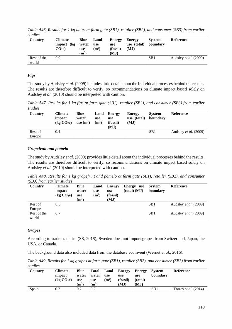
110

Table A46. Results for 1 kg dates at farm gate (SB1), retailer (SB2), and consumer (SB3) from earlier

studies Country Climate

impact (kg

CO2e)

Blue

water

use

(m3)

Land

use

(m2)

Energy

use

(fossil)

(MJ)

Energy

use (total)

(MJ)

System

boundary

Reference

Rest of the

world

0.9 SB1 Audsley et al. (2009)

Figs

The study by Audsley et al. (2009) includes little detail about the individual processes behind the results.

The results are therefore difficult to verify, so recommendations on climate impact based solely on

Audsley et al. (2010) should be interpreted with caution.

Table A47. Results for 1 kg figs at farm gate (SB1), retailer (SB2), and consumer (SB3) from earlier

studies

Country Climate

impact

(kg CO2e)

Blue

water

use (m3)

Land

use

(m2)

Energy

use

(fossil)

(MJ)

Energy

use (total)

(MJ)

System

boundary

Reference

Rest of

Europe

0.4 SB1 Audsley et al. (2009)

Grapefruit and pomelo

The study by Audsley et al. (2009) provides little detail about the individual processes behind the results.

The results are therefore difficult to verify, so recommendations on climate impact based solely on

Audsley et al. (2010) should be interpreted with caution.

Table A48. Results for 1 kg grapefruit and pomelo at farm gate (SB1), retailer (SB2), and consumer

(SB3) from earlier studies Country Climate

impact

(kg CO2e)

Blue

water

use

(m3)

Land

use

(m2)

Energy

use

(fossil)

(MJ)

Energy use

(total) (MJ)

System

boundary

Reference

Rest of

Europe

0.5 SB1 Audsley et al. (2009)

Rest of the

world

0.7 SB1 Audsley et al. (2009)

Grapes

According to trade statistics (SS, 2018), Sweden does not import grapes from Switzerland, Japan, the

USA, or Canada.

The background data also included data from the database ecoinvent (Wernet et al., 2016).

Table A49. Results for 1 kg grapes at farm gate (SB1), retailer (SB2), and consumer (SB3) from earlier

studies

Country Climate

impact

(kg CO2e)

Blue

water

use

(m3)

Total

water

use

(m3)

Land

use

(m2)

Energy

use

(fossil)

(MJ)

Energy

use

(total)

(MJ)

System

boundary

Reference

Spain 0.2 0.2 0.2 SB1 Torres et al. (2014)

111

Switzerland

(origin

Spain)

0.3 0.2 0.3 SB2 Stoessel et al.

(2012)

Japan 0.9 SB2 Yoshikawa et al.

(2008)

USA 0.21/0.24a SB1 Venkat (2012)

Rest of

Europe

0.4 SB1 Audsley et al.

(2009)

Rest of the

world

0.8 SB1 Audsley et al.

(2009)

Canada 0.6b 5.6 SB1 Point et al. (2012)

Spain 0.1/0.2a SB1 Aguilera et al.

(2015)

Italy 0.1b SB1 Cichelli et al.

(2016)

Italy 0.3-0.5b SB1 Bartocci et al.

(2017)

Italy 0.3b SB1 Falcone et al.

(2016)

Swedish

market

0.7 0.08 1.4

SB2 Moberg et al.

(2020) aWine grapes: organic/conventional. bWine grapes, may include several types.

Mangoes

Four studies were found on mangoes. Carneiro et al. (2018), Basset-Mens et al. (2014) and Graefe et al.

(2013) estimated the climate impact to be equal to or below 0.1 kg CO2e per kg for mangoes at farm

gate grown in either Brazil or Colombia. If emissions from transport to Sweden and packaging were

taken into account, the climate impact would be approximately 0.5 kg CO2e per kg mangoes. However,

Audsley et al. (2009) estimated the climate impact to be much higher, 1.8 kg CO2e per kg for mangoes

grown in other parts of the world than Europe and then imported to UK. It is not clear why this result is

particularly higher compared with other results, but one reason could be the emissions that occur from

transporting mangoes to the UK.

Table A50. Results for 1 kg mangoes at farm gate (SB1), retailer (SB2), and consumer (SB3) from earlier

studies

Country Climate

impact (kg

CO2e)

Blue

water

use

(m3)

Land

use

(m2)

Energy

use (fossil)

(MJ)

Energy

use (total)

(MJ)

System

boundary

Reference

Rest of the

worlda

1.8 SB1 Audsley et al.

(2009)

Brazil 0.1 0.4 SB1 Carneiro et al.

(2019)

Brazil 0.1 0.2 1.5 SB1 Basset-Mens et al.

(2014)

Colombia 0.05 SB1 Graefe et al. (2013) aGuavas and mangoes.

Kiwi fruit

New Zealand did not show up in trade statistics (SS, 2018). However, New Zealand exports large

amounts of kiwi fruit (FAOSTAT, 2019) and exports most kiwi fruit to Sweden via other European

countries. The applicability of the study by Nikkhah et al. (2016) was considered to be limited for the

Swedish market, since Iran did not show up in trade statistics (SS, 2018) and Iran imports more kiwi

fruit than it exports according to FAOSTAT (2019).

112

The background data also included data from the database ecoinvent (Wernet et al., 2016).

Table A51. Results for 1 kg kiwi fruit at farm gate (SB1), retailer (SB2), and consumer (SB3) from earlier

studies

Country Climate

impact

(kg

CO2e)

Blue

water

use

(m3)

Land

use

(m2)

Energy use

(fossil) (MJ)

Energy

use

(total)

(MJ)

System

boundary

Reference

New Zealand 0.1-0.2a SB1 Müller et al. (2015)

Rest of Europe 0.4 SB1 Audsley et al.

(2009)

Rest of world 0.9 SB1 Audsley et al.

(2009)

New Zealand 0.3b SB1 McLaren et al.

(2010)

Switzerland

(origin Italy)

0.7 0.1 0.3 SB2 Stoessel et al.

(2012)

Greece 0.7 0.4 0.7 11.1 12.4 SB1 ZEUS (2011)

New Zealand 0.3 Mithraratne (2010)

Italy 0.1 2.7 SB1 Baudino et al.

(2017)

Iran 0.2 SB1 Nikkhah et al.

(2016) aFour scenarios, including two kiwifruit cultivars (green and gold kiwi) and two management systems (integrated and organic

system). bIntegrated production.

Lemons

Three earlier studies were found on lemons. The study by Pergola et al. (2013) showed low results for

lemons grown in Sicily, varying between 0.04 and 0.1 kg CO2e per kg for organic and conventional

farming up to farm gate, respectively. Likewise, the study by Bell et al. (2018) showed low climate

impact for lemons grown in USA, 0.2 kg CO2e per kg. The study by Audsley et al. (2009) showed higher

climate impact, for lemons and limes grown in Europe and then imported to a regional distribution center

in the UK. This is most likely due to the inclusion of transport to Europe. According to Bell et al. (2018),

variations in the results between these studies can also be due to differences in climate, production

practices, and yields.

The background data also included data from the database ecoinvent (Wernet et al., 2016).

Table A52. Results for 1 kg lemons at farm gate (SB1), retailer (SB2), and consumer (SB3) from earlier

studies

Country Climate

impact (kg

CO2e)

Blue

water

use

(m3)

Land

use

(m2)

Energy

use (fossil)

(MJ)

Energy

use (total)

(MJ)

System

boundary

Reference

Sicily 0.04/0.1a 2.10/2.9a SB1 Pergola et al.

(2013a)

Rest of

Europe

0.5b SB1 Audsley et al.

(2009)

USA 0.2 0.2 2.9 SB1 Bell et al. (2018)

Swedish

market

0.5 0.2 0.7 SB2 Moberg et al. (2020)

aOrganic/conventional. bLemons and limes.

Melons (including melons, watermelons, rockmelons etc.)

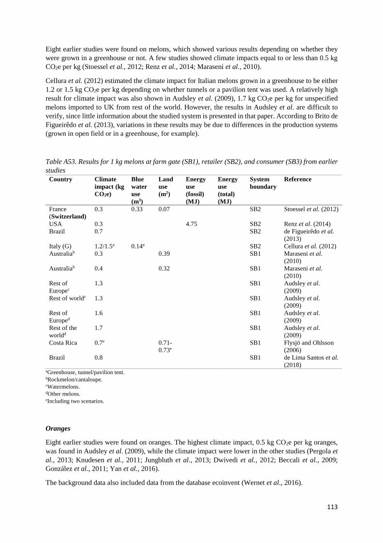
113

Eight earlier studies were found on melons, which showed various results depending on whether they

were grown in a greenhouse or not. A few studies showed climate impacts equal to or less than 0.5 kg

CO2e per kg (Stoessel et al., 2012; Renz et al., 2014; Maraseni et al., 2010).

Cellura et al. (2012) estimated the climate impact for Italian melons grown in a greenhouse to be either

1.2 or 1.5 kg CO2e per kg depending on whether tunnels or a pavilion tent was used. A relatively high

result for climate impact was also shown in Audsley et al. (2009), 1.7 kg CO2e per kg for unspecified

melons imported to UK from rest of the world. However, the results in Audsley et al. are difficult to

verify, since little information about the studied system is presented in that paper. According to Brito de

Figueirêdo et al. (2013), variations in these results may be due to differences in the production systems

(grown in open field or in a greenhouse, for example).

Table A53. Results for 1 kg melons at farm gate (SB1), retailer (SB2), and consumer (SB3) from earlier

studies

Country Climate

impact (kg

CO2e)

Blue

water

use

(m3)

Land

use

(m2)

Energy

use

(fossil)

(MJ)

Energy

use

(total)

(MJ)

System

boundary

Reference

France

(Switzerland)

0.3 0.33 0.07 SB2 Stoessel et al. (2012)

USA 0.3 4.75 SB2 Renz et al. (2014)

Brazil 0.7 SB2 de Figueirêdo et al.

(2013)

Italy (G) 1.2/1.5a 0.14a SB2 Cellura et al. (2012)

Australiab 0.3 0.39 SB1 Maraseni et al.

(2010)

Australiab 0.4 0.32 SB1 Maraseni et al.

(2010)

Rest of

Europec

1.3 SB1 Audsley et al.

(2009)

Rest of worldc 1.3 SB1 Audsley et al.

(2009)

Rest of

Europed

1.6 SB1 Audsley et al.

(2009)

Rest of the

worldd

1.7 SB1 Audsley et al.

(2009)

Costa Rica 0.7e 0.71-

0.73e

SB1 Flysjö and Ohlsson

(2006)

Brazil 0.8 SB1 de Lima Santos et al.

(2018) aGreenhouse, tunnel/pavilion tent. bRockmelon/cantaloupe. cWatermelons. dOther melons. eIncluding two scenarios.

Oranges

Eight earlier studies were found on oranges. The highest climate impact, 0.5 kg CO2e per kg oranges,

was found in Audsley et al. (2009), while the climate impact were lower in the other studies (Pergola et

al., 2013; Knudesen et al., 2011; Jungbluth et al., 2013; Dwivedi et al., 2012; Beccali et al., 2009;

González et al., 2011; Yan et al., 2016).

The background data also included data from the database ecoinvent (Wernet et al., 2016).

114

Table A54. Results for 1 kg oranges at farm gate (SB1), retailer (SB2), and consumer (SB3) from earlier

studies

Country Climate

impact (kg

CO2e)

Blue

water

use

(m3)

Land

use

(m2)

Energy use

(fossil) (MJ)

Energy

use (total)

(MJ)

System

boundary

Reference

Sicily 0.04/0.1a 2.38/2.87a SB1 Pergola et al.

(2013a)

Brazil 0.1b 0.55

&

0.44/

0.50b

0.764 &

0.954/1.265b

SB1 Knudsen et al.

(2011)

Brazil 0.1c SB1 Doublet et al.

(2013)

Spain 0.2d SB1 Doublet et al.

(2013)

USA 0.3 SB1 Doublet et al.

(2013)

USA 0.3 SB1 Dwivedi et al.

(2012)

Rest of

Europe

0.5 SB1 Audsley et al.

(2009)

Italy 0.1 SB1 Beccali et al.

(2009)

USA 0.3 3.7 SB2 González et al.

(2011)

China 0.1 SB1 Yan et al. (2016)

Swedish

market

0.7 0.17 0.68 SB2 Moberg et al.

(2020) aOrganic/conventional. bThree scenarios; organic small vs. large scale/conventional small scale. cTwo scenarios that include organic small and large scale. dIntegrated production. eFour scenarios: organic and integrated.

Papaya

The study by Audsley et al. (2009) provides little detail about the individual processes behind the results.

The results are therefore difficult to verify, so recommendations on climate impact based solely on

Audsley et al. (2010) should be interpreted with caution.

Table A55. Results for 1 kg papaya at farm gate (SB1), retailer (SB2), and consumer (SB3) from earlier

studies

Country Climate

impact (kg

CO2e)

Blue

water

use

(m3)

Land

use

(m2)

Energy

use (fossil)

(MJ)

Energy

use (total)

(MJ)

System

boundary

Reference

Rest of the

world

0.9 SB1 Audsley et al. (2009)

Peaches and nectarines

Eight earlier studies were found on peaches and nectarines, which showed climate impact equal to or

below 0.9 kg CO2e per kg product. The highest climate impact, again, was estimated by Audsley et al.

(2009), where transport from the rest of the world to UK was included in the result. The lowest climate

impact was estimated by Vinyes et al. (2015), who studied a 15-year period (the results are the average

115

for these years). The study by Vinyes et al. (2015) excluded the nursery stage due to lack of data.

Storage, processing, and packaging were also excluded from the study.

Japan does not show up in trade statistics (SS, 2018), and according to FAOSTAT the country has very

little export of peaches. The applicability of the study by Yoshikawa et al. (2008) could therefore be

considered to be limited for the Swedish market.

The background data also included data from the databases ecoinvent (Wernet et al., 2016).

Table A56. Results for 1 kg of peaches and nectarines at farm gate (SB1), retailer (SB2), and consumer

(SB3) from earlier studies

Country Climate

impact (kg

CO2e)

Blue

water

use

(m3)

Total

water

use

(m3)

Land

use

(m2)

Energy

use

(fossil)

(MJ)

Energy

use

(total)

(MJ)

System

boundary

Reference

Japana

0.8 SB2 Yoshikawa et al.

(2008)

Spainb 0.4 0.1 0.1 SB1 Torres et al. (2014)

Rest of

Europe

0.4 SB1 Audsley et al.

(2009)

Rest of

the world

0.9 SB1 Audsley et al.

(2009)

Francea 0.2 0.3 2.5 SB1 Basset-Mens et al.

(2014)

Spainc 0.1-0.3 1.1-2.5 SB1 Vinyes et al. (2015)

Chinaa 0.4 SB1 Yan et al. (2016)

Perua 0.6 SB1 Bartl et al. (2012)

Irana 0.2 SB1 Nikkhah et al.

(2016) aOnly peach. bOnly nectarine. cOnly peach, but four scenarios, where the lowest value corresponds to the high yield scenario and the highest value to the

growth period.

Pears and quinces

The background data also included data from the database ecoinvent (Wernet et al., 2016).

Table A57. Results for 1 kg pears and quinces at farm gate (SB1), retailer (SB2), and consumer (SB3)

from earlier studies

Country Climate

impact

(kg

CO2e)

Blue

water

use

(m3)

Land

use (m2)

Energy

use

(fossil)

(MJ)

Energy

use

(total)

(MJ)

System

boundary

Reference

China

(Beijing

suburb)

0.2/0.4a 2.4-

2.6/2.1a

SB1 Liu et al. (2010)

China

(Liaoning

province)

0.1/0.3b 1.1/1.3b SB1 Liu et al. (2010)

UK 0.6c SB2 Berners-Lee et al. (2012)

Switzerland 0.3 0.03 0.4 SB2 Stoessel et al. (2012)

UK 0.3 SB1 Audsley et al. (2009)

Rest of

Europe

0.4 SB1 Audsley et al. (2009)

Rest of

world

0.9 SB1 Audsley et al. (2009)

China 0.2 SB1 Yan et al. (2016)

116

Portugal 0.1 SB1 de Figueirêdo et al.

(2013)

Italy 0.4 6.7 SB1 Tamburini et al. (2015)

Swedish

market

0.4 0.002 0.5 SB2 Moberg et al. (2020)

Sweden 0.2 0 0.8 SB2 Moberg et al. (2020) aOrganic (incl. 2 scenarios)/conventional (only pears). bOrganic/conventional (only pears). cOnly pears.

Pineapples

Seven earlier LCA studies were found on pineapple production, three of which (Ingwersen, 2012;

Stoessel et al., 2012; Blonk et al., 2010) estimated the climate impact for pineapples grown in Costa

Rica to be equal to or below 0.5 kg CO2e per kg. The system boundary in Blonk et al. (2010) and Stoessel

et al. (2012) included transport from Costa Rica to Europe. The system boundary in Ingwersen (2012)

was from cradle to shelf in the USA, but only the results for the farming stage in Costa Rica are shown

here (Table A58).

The higher climate impact from Audsley et al. (2009) is difficult to explain, since the study gives little

detail on the underlying processes. Usubharatana and Phungrassami (2017), de Ramos and Taboada

(2018), and Graefe et al. (2013) estimated the climate impact to be equal to or below 0.2 kg CO2e per

kg pineapple, where mainly fertilization contributed to the emissions.

The background data also included data from the database ecoinvent (Wernet et al., 2016).

Table A58. Results for 1 kg pineapples at farm gate (SB1), retailer (SB2), and consumer (SB3) from

earlier studies

Country Climate

impact

(kg

CO2e)

Blue

water

use

(m3)

Total

water

use

(m3)

Land

use

(m2)

Energy

use

(fossil)

(MJ)

Energy

use

(total)

(MJ)

System

boundary

Reference

Costa

Rica

0.4 0.02 0.2 SB2 Stoessel et al.

(2012)

Costa

Rica

0.5a SB1 Blonk et al.

(2010)

Costa

Rica

0.2 0.1 1.9 SB2 Ingwersen (2012)

Rest of

the world

1.8 SB1 Audsley et al.

(2009)

Thailand 0.2-0.3b SB1 Usubharatana and

Phungrassami

(2017)

Philip-

pines

0.2 0.9 SB1 De Ramos et al.

(2018)

Colom-

bia

0.1 SB1 Graefe et al.

(2013) aIncluding organic and conventional farming. bIncluding three farms, where the smallest farm had the highest value and the largest farm the lowest value.

Plums and sloes

The study by Audsley et al. (2009) provides little detail about the individual processes behind the results.

The results are therefore difficult to verify, so recommendations on climate impact based solely on

Audsley et al. (2010) should be interpreted with caution.

117

Table A59. Results for 1 kg plums and sloes at farm gate (SB1), retailer (SB2), and consumer (SB3)

from earlier studies

Country Climate

impact

(kg

CO2e)

Blue

water

use (m3)

Land

use

(m2)

Energy

use (fossil)

(MJ)

Energy use

(total) (MJ)

System

boundary

Reference

UK 0.3 SB1 Audsley et al.

(2009)

Rest of

Europe

0.4 SB1 Audsley et al.

(2009)

Rest of

the world

0.9 SB1 Audsley et al.

(2009)

Artichokes

The study by Audsley et al. (2009) provides little detail about the individual processes behind the results.

The results are therefore difficult to verify, so recommendations on climate impact based solely on

Audsley et al. (2010) should be interpreted with caution.

Table A60. Results for 1 kg artichokes at farm gate (SB1), retailer (SB2), and consumer (SB3) from

earlier studies

Country Climate

impact

(kg

CO2e)

Blue

water

use (m3)

Land

use

(m2)

Energy use

(fossil) (MJ)

Energy

use (total)

(MJ)

System

boundary

Reference

Rest of

Europe

0.5 SB1 Audsley et al.

(2009)

Asparagus (including green and white)

Hofer (2009), Schäfer et al. (2014), and Stoessel et al. (2012) studied asparagus production in European

countries and reported climate impact equal to or below 1 kg CO2e per kg. However, Jungbluth et al.

(2016) estimated the climate impact for green asparagus cultivated in Switzerland to be 1.9 kg CO2e per

kg, where the relatively high result could be because of low yield per hectare compared with other

vegetables.

Air transportation can explain the relatively high climate impact figures in Table A61. For example,

asparagus transported by air from Peru to Europe has a climate impact of about 12 kg CO2e per kg

(Hofer, 2009; Jungbluth et al., 2014; Stoessel et al., 2012). According to Jungbluth et al. (2016) Peruvian

asparagus transported via airfreight has a climate impact of 24.9 kg CO2e per kg, which is much higher

than the result presented in Jungbluth et al. (2014). This is possibly due to use of radiative forcing index

(RFI) (N. Jungbluth, personal communication 2019). The RFI factor is multiplied by emissions from

aircraft to calculate the total global warming potential of high-altitude emissions.

The system boundary in Hofer (2009) was not completely clear, so it was assumed to be from cradle to

a Swiss retailer.

The background data also included data from the database ecoinvent (Wernet et al., 2016).

Table A61. Results for 1 kg asparagus at farm gate (SB1), retailer (SB2), and consumer (SB3) from

earlier studies

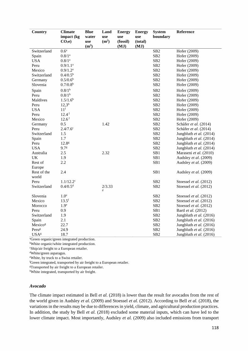
118

Country Climate

impact (kg

CO2e)

Blue

water

use

(m3)

Land

use

(m2)

Energy

use

(fossil)

(MJ)

Energy

use

(total)

(MJ)

System

boundary

Reference

Switzerland 0.6a SB2 Hofer (2009)

Spain 0.8/1a SB2 Hofer (2009)

USA 0.8/1a SB2 Hofer (2009)

Peru 0.9/1.1a SB2 Hofer (2009)

Mexico 0.9/1.2a SB2 Hofer (2009)

Switzerland 0.4/0.5b SB2 Hofer (2009)

Germany 0.5/0.6b SB2 Hofer (2009)

Slovenia 0.7/0.8b SB2 Hofer (2009)

Spain 0.8/1b SB2 Hofer (2009)

Peru 0.8/1b SB2 Hofer (2009)

Maldives 1.5/1.6b SB2 Hofer (2009)

Peru 12,3h SB2 Hofer (2009)

USA 11f SB2 Hofer (2009)

Peru 12.4 f SB2 Hofer (2009)

Mexico 12.6 f SB2 Hofer (2009)

Germany 0.5 1.42 SB2 Schafer et al. (2014)

Peru 2.4/7.6c SB2 Schafer et al. (2014)

Switzerland 1.5 SB2 Jungbluth et al. (2014)

Spain 1.7 SB2 Jungbluth et al. (2014)

Peru 12.8g SB2 Jungbluth et al. (2014)

USA 9.7g SB2 Jungbluth et al. (2014)

Australia 2.5 2.32 SB1 Maraseni et al. (2010)

UK 1.9 SB1 Audsley et al. (2009)

Rest of

Europe

2.2 SB1 Audsley et al. (2009)

Rest of the

world

2.4 SB1 Audsley et al. (2009)

Peru 1.1/12.2c SB2 Stoessel et al. (2012)

Switzerland 0.4/0.5d 2/3.33d

SB2 Stoessel et al. (2012)

Slovenia 1.0e SB2 Stoessel et al. (2012)

Mexico 13.5f SB2 Stoessel et al. (2012)

Morocco 1.9e SB2 Stoessel et al. (2012)

Peru 0.9 SB1 Bartl et al. (2012)

Switzerland 1.9 SB2 Jungbluth et al. (2016)

Spain 2.1 SB2 Jungbluth et al. (2016)

Mexicog 22.7 SB2 Jungbluth et al. (2016)

Perug 24.9 SB2 Jungbluth et al. (2016)

USAg 18.7 SB2 Jungbluth et al. (2016) aGreen organic/green integrated production. bWhite organic/white integrated production. cShip/air freight to a European retailer. dWhite/green asparagus. eWhite, by truck to a Swiss retailer. fGreen integrated, transported by air freight to a European retailer. gTransported by air freight to a European retailer. hWhite integrated, transported by air freight.

Avocado

The climate impact estimated in Bell et al. (2018) is lower than the result for avocados from the rest of

the world given in Audsley et al. (2009) and Stoessel et al. (2012). According to Bell et al. (2018), the

variations in the results may be due to differences in yield, climate, and agricultural production practices.

In addition, the study by Bell et al. (2018) excluded some material inputs, which can have led to the

lower climate impact. Most importantly, Audsley et al. (2009) also included emissions from transport

119

when importing avocados to a regional distribution center in the UK, and Stoessel et al. (2012) included

transport distance between Israel and Switzerland, likely explaining the higher impacts estimated in

these studies.

Use of blue water (irrigation water), estimated by Bell et al. (2018) and Stoessel et al. (2012) to be 0.60

and 0.93 m3/kg, respectively, is in line with the California average use (0.62 m3/kg) and the country

average use in Israel (0.70 m3/kg) for avocado (Mekonnen et al., 2011). However, according to trade

statistics (SS, 2018), Sweden does not import avocados from USA, and the USA imports more avocados

than it exports. Therefore, the applicability of the study by Bell et al. (2018) can be considered limited

for the Swedish market.

The background data also included data from the database ecoinvent (Wernet et al., 2016).

Table A62. Results for 1 kg avocado at farm gate (SB1), retailer (SB2), and consumer (SB3) from earlier

studies

Country Climate

impact

(kg CO2e)

Blue

water

use

(m3)

Land use

(m2)

Energy

use

(fossil)

(MJ)

Energy

use

(total)

(MJ)

System

boundary

Reference

Rest of

Europe

0.4 SB2 Audsley et al. (2009)

Rest of the

world

0.9 SB2 Audsley et al. (2009)

Israel 1.3 0.93 1.0 SB2 Stoessel et al. (2012)

USA 0.5 0.60 6.70 SB1 Bell et al. (2018)

Peru 0.5 SB1 Bartl et al. (2012)

Colombia 0.2 SB1 Graefe et al. (2013) aOrganic/conventional.

Broccoli

Seven earlier LCA studies were found on broccoli. González et al. (2011) studied broccoli from Sweden,

showing a climate impact of 0.4 kg CO2e per kg, while Moberg et al. (2020) estimated a slightly higher

climate impact. Similar results were shown for broccoli from UK, Switzerland, and USA (Stoessel et

al., 2012; Venkat, 2012; i Canals et al., 2008). Jungbluth et al. (2016) estimated higher climate impacts

of 0.6, 0.7 and 0.9 kg CO2e per kg for broccoli grown in Switzerland, Italy, and Spain, respectively,

where transport to a Swiss retailer was included.

Maraseni et al. (2010) estimated the highest climate impact for broccoli, 1.7 kg CO2e per kg. However,

according to trade statistics (SS, 2018), Sweden does not import broccoli from Australia. Furthermore,

Australia imports more broccoli than it exports (FAOSTAT, 2019). Therefore, the applicability of the

study by Maraseni et al. (2010) can be considered limited for the Swedish market.

The system boundary in i Canals et al. (2008) is from cradle to grave, but the retail to grave phase is

excluded in the results shown in Table A63.

The background data also included data from the database ecoinvent (Wernet et al., 2016).

Table A63. Results for 1 kg broccoli at farm gate (SB1), retailer (SB2), and consumer (SB3) from earlier

studies

Country Climate

impact

(kg CO2e)

Blue

water

use (m3)

Land

use (m2)

Energy

use

(fossil)

(MJ)

Energy

use

(total)

(MJ)

System

boundary

Reference

Sweden 0.4 3.60 SB2 González et al. (2011)

120

UKa 0.4-0.5 0.50-

0.63

5.50-

6.00

SB3 i Canals et al. (2008)

Spaina 0.7-1.1 0.11-

0.25

0.01-

0.04

13.00-

17.00

SB3 i Canals et al. (2008)

Switzerland 0.5 0.03 0.10 SB2 Stoessel et al. (2012)

USA 0.4b SB1 Venkat (2012)

Switzerland 0.6 SB2 Jungbluth et al.

(2016)

Italy 0.7 SB2 Jungbluth et al.

(2016)

Spain 0.9 SB2 Jungbluth et al.

(2016)

Switzerland

(F)c

0.66 SB2 Jungbluth et al.

(2016)

Australia 1.7 1.55 SB1 Maraseni et al. (2010)

Swedish

market

0.6 SB2 Moberg et al. (2020)

Sweden 0.6 0.01 1.4 SB2 Moberg et al. (2020) aIncluding four scenarios. bIncluding organic and conventional broccoli. cDeep frozen.

Cabbage

Three earlier studies estimated climate impact for cabbage or kale grown in Sweden, which was

estimated to be equal to or below 0.3 kg CO2e per kg (Moberg et al., 2020; Landqvist & Woodhouse,

2015; González et al., 2011). Audsley et al. (2009) estimated the highest climate impact for imported

cabbage to the UK from rest of the world, where emissions from transport probably play a significant

role.

The background data also included data from the database ecoinvent (Wernet et al., 2016).

Table A64. Results for 1 kg cabbage at farm gate (SB1), retailer (SB2), and consumer (SB3) from earlier

studies

Country Climate

impact

(kg CO2e)

Blue

water

use

(m3)

Land

use

(m2)

Energy

use

(fossil)

(MJ)

Energy use

(total) (MJ)

System

boundary

Reference

Sweden 0.1 1.10 SB2 González et al. (2011)

Australia 0.2 0.25 SB1 Maraseni et al. (2010)

Japan 0.4 SB2 Yoshikawa et al.

(2008)

UK 0.2 SB1 Audsley et al (2009)

Rest of

Europe

0.5 SB1 Audsley et al. (2009)

Rest of the

world

0.6 SB1 Audsley et al. (2009)

Swedish

market

0.4 0.03 0.71 SB2 Moberg et al. (2020)

Sweden 0.3 0.01 0.3 SB2 Moberg et al. (2020)

Swedena 0.2 SB1 Landqvist et al. (2014)

China 0.1 SB1 Yue et al. (2017) aKale.

Capsicums/peppers

Seven earlier LCA studies were found on capsicums/peppers. Yoshikawa et al. (2008) estimated the

highest climate impact, for green peppers grown in a greenhouse. The heat source was not specified in

121

the study. According to the same study, green peppers grown in the open field have a climate impact of

0.7 kg CO2e per kg.

The background data also included data from the database ecoinvent (Wernet et al., 2016).

Table A65. Results for 1 kg capsicums/peppers at farm gate (SB1), retailer (SB2), and consumer (SB3)

from earlier studies (G: greenhouse)

Country Climate

impact

(kg

CO2e)

Blue water

use (m3)

Land

use

(m2)

Energy

use

(fossil)

(MJ)

Energy

use

(total)

(MJ)

System

boundary

Reference

Australia 0.2 0.38 SB1 Maraseni et al. (2010)

Japan 0.7 SB2 Yoshikawa et al.

(2008)

Japan (G) 3.8 SB2 Yoshikawa et al.

(2008)

Rest of the

world

0.9 SB1 Audsley et al. (2009)

Greece 0.16/0.09a 0.40/

0.25a

Chatzisymeon et al.

(2017)

Switzerlandb (G) 0.9 0.04 0.06 SB2 Stoessel et al. (2012)

Italy (G) 1.1/1.2c 0.11/0.10d SB2 Cellura et al. (2012)

China 0.2 SB1 Yue et al. (2017) aOrganic/conventional. bGreenhouse, fuel heating oil. cGreenhouse tunnel/pavilion tent.

Cauliflower

Results from the study by Audsley et al. (2009) showed much higher climate impact than other studies.

However, that study presents little information about the underlying processes, and the difference is

therefore difficult to explain.

The background data also included data from the database ecoinvent (Wernet et al., 2016).

Table A66. Results for 1 kg cauliflowers at farm gate (SB1), retailer (SB2), and consumer (SB3) from

earlier studies

Country Climate

impact (kg

CO2e)

Blue

water

use (m3)

Land

use

(m2)

Energy

use

(fossil)

(MJ)

Energy

use

(total)

(MJ)

System

boundary

Reference

Netherlands 0.34/0.28a SB1 Blonk et al. (2010)

Australia 0.4 0.51 SB1 Maraseni et al.

(2010)

Switzerland 0.4 0.03 0.11 SB2 Stoessel et al.

(2012)

UKb 1.9 SB1 Audsley et al.

(2009)

Rest of Europeb 2.2 SB1 Audsley et al.

(2009)

Rest of the

worldb

2.4 SB1 Audsley et al.

(2009)

China 0.1 SB1 Yue et al. (2017)

Swedish market 0.5 0.05 0.68 SB2 Moberg et al.

(2020)

Sweden 0.4 0.7 0.01 SB2 Moberg et al.

(2020) aOrganic/conventional. bCauliflowers and broccoli.

122

Celery

Only two earlier LCA studies were found on celery (Bell et al., 2018; Maraseni et al., 2010), which

estimated the climate impact to be below 0.2 kg CO2e per kg. The background data also included data

from the database ecoinvent (Wernet et al.. 2016), which showed somewhat higher results.

Table A67. Results for 1 kg celery at farm gate (SB1), retailer (SB2), and consumer (SB3) from earlier

studies

Country Climate

impact (kg

CO2e)

Blue

water

use (m3)

Land use

(m2)

Energy

use

(fossil)

(MJ)

Energy

use

(total)

(MJ)

System

boundary

Reference

USA 0.1 0.10 1.70 SB1 Bell et al.

(2018)

Australia 0.2 0.20 SB1 Maraseni et al.

(2009)

Chillies

Table A68. Results for 1 kg chillies at farm gate (SB1), retailer (SB2), and consumer (SB3) from earlier

studies

Country Climate

impact (kg

CO2e)

Land use

(m2)

Energy

use

(fossil)

(MJ)

Energy

use

(total)

(MJ)

System

boundary

Reference

Australia 0.7 0.98 SB1 Maraseni et al. (2010)

Rest of Europe 1.3a SB1 Audsley et al. (2009) aChillies and peppers, dry.

Cucumbers and gherkins

Results from Marton et al. (2010) show that cucumbers grown in greenhouses heated with fuel oil can

have a much higher climate impact (in this study around 1.7 kg CO2e per kg cucumber) than when grown

in greenhouses heated with waste heat where no fossil fuel is used (0.2 kg CO2e per kg cucumber).

Cucumbers grown in open fields in Sweden have a climate impact of 0.1 kg CO2e per kg, according to

González et al. (2011). According to the same study, cucumbers grown in greenhouses have a much

higher impact if the greenhouse is heated with fuel oil instead of electricity.

The system boundary in Hofer (2009) was assumed to be up to a Swiss retailer.

The background data also included data from the database ecoinvent (Wernet et al., 2016).

Table A69. Results for 1 kg cucumber and gherkins (only cucumbers if not specified) at farm gate (SB1),

retailer (SB2), and consumer (SB3) from earlier studies (G: greenhouse) Country Climate

impact (kg

CO2e)

Blue

water

use

(m3)

Land

use

(m2)

Energy

use

(fossil)

(MJ)

Energy

use

(total)

(MJ)

System

boundary

Reference

Sweden 0.1 SB2 González et al. (2011)

Australia 0.1 0.14 SB1 Maraseni et al. (2010)

Austria 0.2a SB2 Lindenthal et al. (2010)

Switzerland (G) 0.2b SB2 Marton et al. (2010)

Switzerland (G) 1.3c SB2 Stoessel et al. (2012)

Sweden (G) 2.6d 35 SB2 González et al. (2011)

123

Sweden (G) 0.75g 41 SB2 González et al. (2011)

Switzerland (G) 1.7d SB2 Marton et al. (2010)

UK (G) 3.8c SB1 Audsley et al. (2009)

Switzerland 0.1/0.2e SB2 Hofer (2009)

Belgium 0.2/0.3e SB2 Hofer (2009)

Netherlands 0.2/0.3e SB2 Hofer (2009)

Spain 0.3 SB2 Hofer (2009)

Switzerland (G) 2f SB2 Hofer (2009)

Belgium (G) 2.1f SB2 Hofer (2009)

Netherlands (G) 2.1f SB2 Hofer (2009)

China 0.1/0.2h SB1 Yue et al. (2017)

Sweden 0.7 0.02 0.1 SB2 Moberg et al. (2020)

Swedish market 0.7 0.01 0.1 SB2 Moberg et al. (2020) aOrganic and conventional. bGreenhouse heated from waste heat. cGreenhouse, heat not specified. dPlastic greenhouse heated with fuel oil. eGherkins, organic/conventional. fGherkins, greenhouse, integrated production, unspecified heated greenhouse. gGreenhouse, electricity heating. hGreenhouse/open field.

Eggplants (aubergines)

The studies showing a higher impact (Wernet et al., 2016; Stoessel et al., 2012) studied production in

heated greenhouses. There was not sufficient background information in Audsley et al. (2009) to explain

the results.

The background data also included data from the database ecoinvent (Wernet et al., 2016).

Table A70. Results for 1 kg eggplants (aubergines) at farm gate (SB1), retailer (SB2), and consumer

(SB3) from earlier studies (G: greenhouse) Country Climate

impact (kg

CO2e)

Blue

water

use (m3)

Land

use

(m2)

Energy

use

(fossil)

(MJ)

Energy

use

(total)

(MJ)

System

boundary

Reference

Rest of Europe 1.3 SB1 Audsley et al. (2009)

Switzerland (G)a 1.4 0.05 0.06 SB2 Stoessel et al. (2012)

China 0.2/0.3c SB1 Yue et al. (2017) aGreenhouse heated. bOpen field/greenhouse.

Fennel

The background data also included data from the database ecoinvent (Wernet et al., 2016).

Table A71. Results for 1 kg fennel at farm gate (SB1), retailer (SB2), and consumer (SB3) from earlier

studies

Country Climate

impact (kg

CO2e)

Blue

water

use

(m3)

Land

use

(m2)

Energy

use

(fossil)

(MJ)

Energy

use

(total)

(MJ)

System

boundary

Reference

Switzerland 0.5 0.05 0.14 SB2 Stoessel et al. (2012)

Garlic

124

Earlier studies show that garlic likely has a climate impact below 1 kg CO2e per kg. For example, garlic

from Iran has an impact of 0.4 kg CO2e per kg (Khoshnevisan & Rafiee, 2014). However, if packaging

and transport to Sweden were added, the climate impact would be 0.9 kg CO2e per kg. European

production was considered most relevant for the Swedish market.

The background data also included data from the database ecoinvent (Wernet et al., 2016).

Table A72. Results for 1 kg garlic at farm gate (SB1), retailer (SB2), and consumer (SB3) from earlier

studies

Country Climate

impact (kg

CO2e)

Land

use

(m2)

Energy use

(fossil)

(MJ)

Energy

use

(total)

(MJ)

System

boundary

Reference

UK 0.6 SB1 Audsley et al. (2009)

Rest of Europe 0.7 SB1 Audsley et al. (2009)

Czech Republic 0.2/0.4a SB1 Moudrý jr et al. (2016)

Iran 0.4 SB1 Khoshnevisan and Rafiee

(2014) aOrganic/conventional.

Ginger

The study by Audsley et al. (2009) provides little detail about the individual processes behind the results.

The results are therefore difficult to verify, so recommendations on climate impact based solely on

Audsley et al. (2010) should be interpreted with caution.

Table A73. Results for 1 kg ginger at farm gate (SB1), retailer (SB2), and consumer (SB3) from earlier

studies

Country Climate

impact (kg

CO2e)

Land

use

(m2)

Energy use

(fossil)

(MJ)

Energy

use

(total)

(MJ)

System

boundary

Reference

Rest of the

world

0.9 SB1 Audsley et al. (2009)

Green beans

Sweden has no significant production of green beans for the retailer market, and no earlier study could

be found on green beans produced in Sweden.

Table A74. Results for 1 kg green beans at farm gate (SB1), retailer (SB2), and consumer (SB3) from

earlier studies (F: fresh, FZ: frozen, C: canned) Country Climate

impact (kg

CO2e)

Land

use

(m2)

Energy use

(fossil) (MJ)

Energy use

(total) (MJ)

System

boundary

Reference

Spain (F) 0.1-0.3a SB1 Romero-Gámez et al.

(2012)

The

Netherlands

(C)

1.3-1.6b SB2 Blonk et al. (2010)

UK (F) 1.6 SB1 Audsley et al. (2009)

UK (F)c 0.08-0.13 0.08-

0.13

1.21 20.1-22.4 SB3 i Canals et al. (2008)

UK (FZ) 0.1 0.10 1.14 27.7 SB3 i Canals et al. (2008)

Kenya (F)d 10.7 0.16 0.48 158.2 SB3 i Canals et al. (2008)

Uganda (F)d 10.9 0.09 0.82 158.2 SB3 i Canals et al. (2008)

Australia (F) 1.4 1.73 SB1 Maraseni et al. (2010)

125

aSix scenarios for three treatment over two years. Data presented as average for the two years. One year for one treatment

(greenhouse with misting) resulted in much higher climate impact than the other scenarios due to very low yield that year. bTwo scenarios, one canned in glass jar (higher value) and one in tin can (lower value), cTwo scenarios for UK. dTransported by air to UK.

Lettuce

The particularly high climate impact estimated by i Canals et al. (2008) corresponded to lettuce grown

in a greenhouse year-round heated with natural gas. Lettuce in open fields showed lower climate impact,

equal to or below 0.6 kg CO2e per kg. It is unclear why the climate impact from the study by Audsley

et al. (2009) (rest of the world) is so much higher, but a likely explanation is use of heated greenhouse

and possibly high waste rates when traded from outside Europe. For the Swedish market, European

production was considered most relevant.

The background data also included data from the database ecoinvent (Wernet et al., 2016).

Table A75. Results for 1 kg lettuce at farm gate (SB1), retailer (SB2), and consumer (SB3) from earlier

studies (G: greenhouse)

Country Climate

impact (kg

CO2e)

Blue

water

use

(m3)

Land

use

(m2)

Energy

use

(fossil)

(MJ)

Energy

use

(total)

(MJ)

System

boundary

Reference

Sweden 0.1 1.40 SB2 González et al. (2011)

Holland 0.1 1.30 SB2 González et al. (2011)

USA 0.3 3.90 SB2 González et al. (2011)

UKa 0.2-0.5 0.04-

0.10

0.25-

0.44

5-11 SB2 i Canals et al. (2008)

Spainb 0.4-0.6 0.04-

0.13

0.20-

0.24

10-11 SB2 i Canals et al. (2008)

UK (G)c 1.3 0.01 0.08 31 SB2 i Canals et al. (2008)

UK (G)d 4.7 0.05 0.08 105 SB2 i Canals et al. (2008)

Australia 0.3 0.37 SB1 Maraseni et al. (2010)

UK 0.3 SB1 Hospido et al. (2009)

Spain 0.3 SB1 Hospido et al. (2009)

UK (G)d 1.5-3.7 SB1 Hospido et al. (2009)

USA 0.3/0.2e SB1 Venkat (2012)

Sweden 0.4 SB2 Strid and Eriksson

(2014)

Switzerland (G) 0.5/4.5f SB2 Marton et al. (2010)

Japan 0.6 SB2 Yoshikawa et al. (2008)

UKg 1.2 SB1 Audsley et al. (2009)

Rest of Europeg 1 SB1 Audsley et al. (2009)

Rest of the

worldg

10 SB1 Audsley et al. (2009)

Australia 3.6 SB2 Gunady et al. (2012)

Italyh 0.3 4.12 SB1 Tamburini et al. (2015)

Swedish market 0.3 0.01 0.48 SB2 Moberg et al. (2020)

Sweden 0.3 0.5 0.02 SB2 Moberg et al. (2020) aIncluding five scenarios (different farms). bIncluding four scenarios (different farms). cBoth indoor and outdoor growing (glass greenhouse with natural gas heating). dGlass greenhouse year round with natural gas heating. eOrganic/conventional. fGreenhouse from waste heat/plastic greenhouse with fuel heating oil. gLettuce and chicory. hLettuce and chicory.

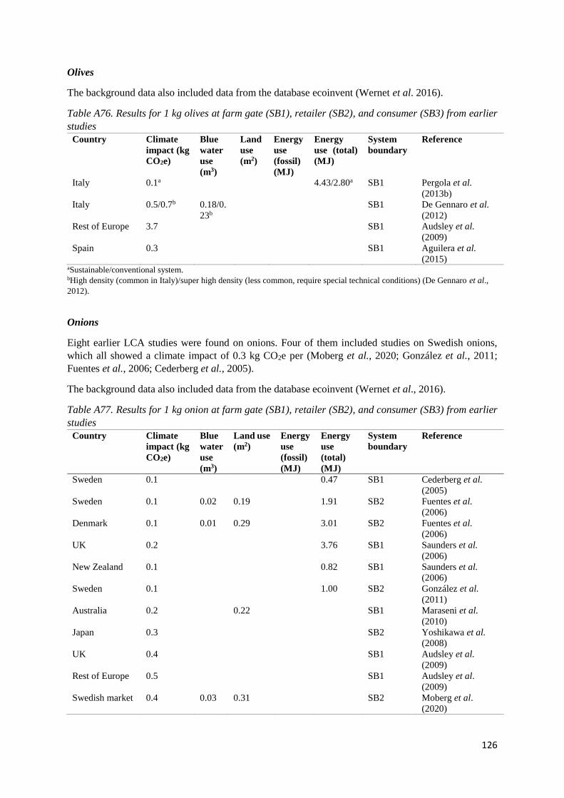
126

Olives

The background data also included data from the database ecoinvent (Wernet et al. 2016).

Table A76. Results for 1 kg olives at farm gate (SB1), retailer (SB2), and consumer (SB3) from earlier

studies

Country Climate

impact (kg

CO2e)

Blue

water

use

(m3)

Land

use

(m2)

Energy

use

(fossil)

(MJ)

Energy

use (total)

(MJ)

System

boundary

Reference

Italy 0.1a 4.43/2.80a SB1 Pergola et al.

(2013b)

Italy 0.5/0.7b 0.18/0.

23b

SB1 De Gennaro et al.

(2012)

Rest of Europe 3.7 SB1 Audsley et al.

(2009)

Spain 0.3 SB1 Aguilera et al.

(2015) aSustainable/conventional system. bHigh density (common in Italy)/super high density (less common, require special technical conditions) (De Gennaro et al.,

2012).

Onions

Eight earlier LCA studies were found on onions. Four of them included studies on Swedish onions,

which all showed a climate impact of 0.3 kg CO2e per (Moberg et al., 2020; González et al., 2011;

Fuentes et al., 2006; Cederberg et al., 2005).

The background data also included data from the database ecoinvent (Wernet et al., 2016).

Table A77. Results for 1 kg onion at farm gate (SB1), retailer (SB2), and consumer (SB3) from earlier

studies

Country Climate

impact (kg

CO2e)

Blue

water

use

(m3)

Land use

(m2)

Energy

use

(fossil)

(MJ)

Energy

use

(total)

(MJ)

System

boundary

Reference

Sweden 0.1 0.47 SB1 Cederberg et al.

(2005)

Sweden 0.1 0.02 0.19 1.91 SB2 Fuentes et al.

(2006)

Denmark 0.1 0.01 0.29 3.01 SB2 Fuentes et al.

(2006)

UK 0.2 3.76 SB1 Saunders et al.

(2006)

New Zealand 0.1 0.82 SB1 Saunders et al.

(2006)

Sweden 0.1 1.00 SB2 González et al.

(2011)

Australia 0.2 0.22 SB1 Maraseni et al.

(2010)

Japan 0.3 SB2 Yoshikawa et al.

(2008)

UK 0.4 SB1 Audsley et al.

(2009)

Rest of Europe 0.5 SB1 Audsley et al.

(2009)

Swedish market 0.4 0.03 0.31 SB2 Moberg et al.

(2020)

127

Sweden 0.3 0.03 0.25 SB2 Moberg et al.

(2020)

Pumpkins

The system boundary in Schäfer and Blanke (2012) is up to a German retailer, so emissions from

transport between Argentina and Germany are accounted for in the result. Data from Audsley et al.

(2009) were difficult to verify due to limited background information in the report.

Table A78. Results for 1 kg pumpkin at farm gate (SB1), retailer (SB2), and consumer (SB3) from earlier

studies

Country Climate

impact (kg

CO2e)

Blue

water

use (m3)

Land use

(m2)

Energy

use

(fossil)

(MJ)

Energy

use

(total)

(MJ)

System

boundary

Reference

Germany 0.04a SB2 Schäfer and

Blanke (2012)

Argentina 0.1 SB2 Schäfer and

Blanke (2012)

Australia 0.3 0.58 SB1 Maraseni et

al. (2010)

Rest of Europe 2.2b SB1 Audsley et al.

(2009) aIncluding organic and integrated production, where organic production had a slightly higher impact than integrated. bPumpkins, squash and gourds.

Spinach

Data from Audsley et al. (2009) were difficult to verify due to limited background information in the

report.

The background data also included data from the database ecoinvent (Wernet et al., 2016).

Table A79. Results for 1 kg spinach at farm gate (SB1), retailer (SB2), and consumer (SB3) from earlier

studies

Country Climate

impact (kg

CO2e)

Blue

water

use (m3)

Land

use

(m2)

Energy

use

(fossil)

(MJ)

Energy

use

(total)

(MJ)

System

boundary

Reference

Switzerland 0.2 0.01 0.04 SB2 Stoessel et al.

(2012)

Japan 0.9 SB2 Yoshikawa et

al. (2008)

Rest of Europe 2.2 SB1 Audsley et al.

(2009)

Tomatoes

Many LCA studies were found on tomatoes, as listed in Table A80. Regarding tomato production in

Sweden, the data from Moberg et al. (2020) were considered most relevant, because the energy sources

for heating greenhouses have changed in recent years. In general, heating source for heating greenhouses

is important for the climate impact results. For tomatoes produced in unheated greenhouses, the transport

distance or materials such as plastic for covering the greenhouse can be more important for the climate

impact (Röös & Karlsson, 2013).

128

The background data also included data from the database ecoinvent (Wernet et al., 2016).

Table A80. Results for 1 kg tomatoes at farm gate (SB1), retailer (SB2), and consumer (SB3) from earlier

studies (G: greenhouse)

Country Climate

impact (kg

CO2e)

Blue

water

use

(m3)

Land

use

(m2)

Energy

use

(fossil)

(MJ)

Energy

use (total)

(MJ)

System

boundary

Reference

World 0.2 SB3 Andersson

(2000)

Switzerland 0.3/0.2a SB2 Hofer (2009)

Belgium 0.4/0.3a SB2 Hofer (2009)

Netherlands 0.4/0.3a SB2 Hofer (2009)

Spain 0.4/0.4a SB2 Hofer (2009)

Maldives 0.5/0.5a SB2 Hofer (2009)

Belgium (G) 1b SB2 Hofer (2009)

Switzerland (G) 1.1b SB2 Hofer (2009)

Australia 0.2 0.25 SB1 Maraseni et al.

(2010)

Sweden 0.2 0.09 3.30 SB2 Röös and

Karlsson (2013)

Sweden (G) 0.3c 0.02 6.80 SB2 Röös and

Karlsson (2013)

Sweden (origin

Netherlands (G))

1.0d 0.02 16 SB2 Röös and

Karlsson (2013)

Sweden (origin

Spain)

0.5 0.08 8.60 SB2 Röös and

Karlsson (2013)

USA 0.3 3.70 SB2 González et al.

(2011)

Spain 0.4 3 SB2 González et al.

(2011)

Netherlands (G) 2.8 49 SB2 González et al.

(2011)

Sweden (G) 3.7 51 SB2 González et al.

(2011)

Austria 0.2/0.2a SB2 Lindenthal et al.

(2010)

Spain 0.2-0.3e 2.9-4.8e

(CED)

SB1 Sanyé-Mengual

et al. (2014)

Morocco 0.2 3.61 SB1 Payen et al.

(2015)

France (origin

Morocco)

0.6 9.13 SB1 Payen et al.

(2015)

Spain 0.3f 4 (CED) SB1 Torrellas et al.

(2012a)

Spainf (G) 0.3 4 (CED) SB1 Torrellas et al.

(2012b)

Hungaryg (G) 0.4 6.9 (CED) SB1 Torrellas et al.

(2012b)

Netherlandsh (G) 0.8 12 (CED) SB1 Torrellas et al.

(2012b)

Netherlandsi (G) 2.0 31 SB1 Torrellas et al.

(2012b)

Hungaryj (G) 5.0 87 SB1 Torrellas et al.

(2012b)

Australia (G) 0.4/1.9k 0.04/0

0.02k

SB1 Page et al.

(2012)

Australia 0.3 0.05 SB1 Page et al.

(2012)

129

Australia (G) 1.7l 0.04l SB1 Page et al.

(2012)

USA 0.5 7.05 SB2 Renz et al.

(2014)

France 0.5m SB1 Boulard et al.

(2011)

France (G) 1.6-2.4n SB1 Boulard et al.

(2011)

Switzerland 0.7 0.03 0.02 SB2 Stoessel et al.

(2012)

Japan 0.8 SB2 Yoshikawa et al.

(2008)

Spain (G) 1o SB1 Blonk et al.

(2010)

Netherlands (G) 1.1o SB1 Blonk et al.

(2010)

Netherlands (G) 2.2o

(organic)

SB1 Blonk et al.

(2010)

Sweden (G) 2.7p 0.02 0.02 51 SB2 Fuentes et al.

(2006)

Netherlands (G) 2.9p 53.40 SB2 Fuentes et al.

(2006)

Denmark (G) 3.7p 0.02 0.02 61.91 SB2 Fuentes et al.

(2006)

Sweden (G) 3.3p 42 SB2 Carlsson-

Kanyama (1998)

UK (G) 3.8 SB1 Audsley et al.

(2009)

UK (G) 6.1

(unspecified

heated)

SB2 Berners-Lee et

al. (2012)

UK (G) 2.2q 0.02 0.02 36 SB1 Williams et al.

(2008)

UK (G) 5.1r 0.06 0.04 83 SB1 Williams et al.

(2008)

UK (G) 5.9s 0.07 0.05 95 SB1 Williams et al.

(2008)

Italy (organic) 0.1 0.87 SB1 Tamburini et al.

(2015)

China 0.1/0.2t SB1 Yue et al. (2017)

Swedish market 1.4 0.01 0.08 SB2 Moberg et al.

(2020)

Sweden 0.9 0.03 0.002 SB2 Moberg et al.

(2020) aOrganic/integrated production. bHeated greenhouse (GH) (heat not specified), integrated production. cHeated GH using mostly renewable energy. dHeated GH using mostly natural gas. eRooftop GH, no auxiliary heat. Including three scenarios. fMulti-tunnel GH. gVenlo GH with no auxiliary heating (thermal energy). hVenlo GH with avoided electricity at combined heat and power plant (CHP). iVenlo GH with energy allocation at CHP. jVenlo GH with natural gas. kGH “low tech summer” with no auxiliary heating systems/GH “high tech year” with natural gas and coal. lGH “mid tech year” with coal. mTunnel GH with no auxiliary heating systems. nEight scenarios, including plastic and glass greenhouse and tunnel, highest value corresponds to “Plastic North vine” with

mainly natural gas. oGH, natural gas heating. pSweden and Netherlands: fuel heating oil. Denmark: LPG and electricity heating.

130

qHeated GH for classic loose tomato, using a natural gas boiler-heater. rHeated GH for classic vine tomato, using a natural gas boiler-heater. sHeated GH for baby plum tomato, using a natural gas boiler-heater. tOpen field/greenhouse.

Zucchini/button squash

The system boundary in the study by Jungbluth et al. (2016) is not clear, but was assumed to be from

cradle to a Swiss retailer (including packing).

The background data also included data from the database ecoinvent (Wernet et al., 2016).

Table A81. Results for 1 kg zucchini at farm gate (SB1), retailer (SB2), and consumer (SB3) from earlier

studies (G: greenhouse)

Country Climate

impact (kg

CO2e)

Blue

water

use (m3)

Land

use

(m2)

Energy

use

(fossil)

(MJ)

Energy

use

(total)

(MJ)

System

boundary

Reference

Sweden 0.1 0.96 SB2 González et al.

(2011)

Austria 0.18/0.22a SB2 Lindenthal et al.

(2010)

Australia 1.2 1.03 SB1 Maraseni et al.

(2010)

Italy (G) 1.6/1.9b 0.16/0.15b

SB2 Cellura et al. (2012)

Switzerland 0.6 SB2 Jungbluth et al.

(2016)

Switzerland

(G)

3.9c SB2 Jungbluth et al.

(2016)

Spain 0.9 SB2 Jungbluth et al.

(2016)

Italy 0.7 SB2 Jungbluth et al.

(2016)

Morocco 1.0 SB2 Jungbluth et al.

(2016) aOrganic/conventional. bGreenhouse, tunnel/pavilion with no auxiliary heating systems. cGreenhouse heated with fuel oil.

Blueberries

No earlier studies were found on wild berries. All data included are for cultivated blueberries.

Table A82. Results for 1 kg blueberries at farm gate (SB1), retailer (SB2), and consumer (SB3) from

earlier studies

Country Climate

impact (kg

CO2e)

Land use

(m2)

Energy

use

(fossil)

(MJ)

Energy

use

(total)

(MJ)

System

boundary

Reference

USA 0.7/0.8a SB1 Venkat (2012)

Rest of the

world

1.4 SB1 Audsley et al. (2009)

Italy 0.2 3.55 SB2 Girgenti et al. (2013)

Italy 0.4 8.98 SB2 Peano et al. (2015)

Chile 0.3-0.7b SB1 Cordes et al. (2016) aOrganic/conventional. bOrganic, including results for five different orchards with varying fertilizer application.

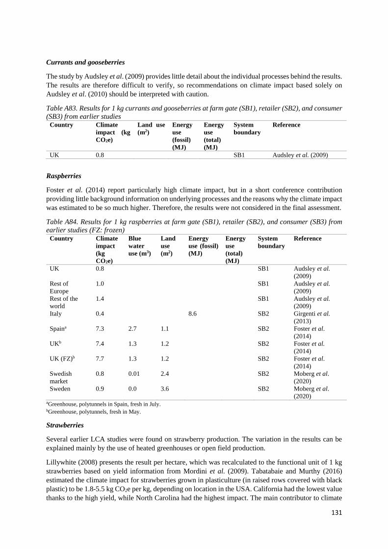
131

Currants and gooseberries

The study by Audsley et al. (2009) provides little detail about the individual processes behind the results.

The results are therefore difficult to verify, so recommendations on climate impact based solely on

Audsley et al. (2010) should be interpreted with caution.

Table A83. Results for 1 kg currants and gooseberries at farm gate (SB1), retailer (SB2), and consumer

(SB3) from earlier studies Country Climate

impact (kg

CO2e)

Land use

(m2)

Energy

use

(fossil)

(MJ)

Energy

use

(total)

(MJ)

System

boundary

Reference

UK 0.8 SB1 Audsley et al. (2009)

Raspberries

Foster et al. (2014) report particularly high climate impact, but in a short conference contribution

providing little background information on underlying processes and the reasons why the climate impact

was estimated to be so much higher. Therefore, the results were not considered in the final assessment.

Table A84. Results for 1 kg raspberries at farm gate (SB1), retailer (SB2), and consumer (SB3) from

earlier studies (FZ: frozen)

Country Climate

impact

(kg

CO2e)

Blue

water

use (m3)

Land

use

(m2)

Energy

use (fossil)

(MJ)

Energy

use

(total)

(MJ)

System

boundary

Reference

UK 0.8 SB1 Audsley et al.

(2009)

Rest of

Europe

1.0 SB1 Audsley et al.

(2009)

Rest of the

world

1.4 SB1 Audsley et al.

(2009)

Italy 0.4 8.6 SB2 Girgenti et al.

(2013)

Spaina 7.3 2.7 1.1 SB2 Foster et al.

(2014)

UKb 7.4 1.3 1.2 SB2 Foster et al.

(2014)

UK (FZ)b 7.7 1.3 1.2 SB2 Foster et al.

(2014)

Swedish

market

0.8 0.01 2.4 SB2 Moberg et al.

(2020)

Sweden 0.9 0.0 3.6 SB2 Moberg et al.

(2020) aGreenhouse, polytunnels in Spain, fresh in July. bGreenhouse, polytunnels, fresh in May.

Strawberries

Several earlier LCA studies were found on strawberry production. The variation in the results can be

explained mainly by the use of heated greenhouses or open field production.

Lillywhite (2008) presents the result per hectare, which was recalculated to the functional unit of 1 kg

strawberries based on yield information from Mordini et al. (2009). Tabatabaie and Murthy (2016)

estimated the climate impact for strawberries grown in plasticulture (in raised rows covered with black

plastic) to be 1.8-5.5 kg CO2e per kg, depending on location in the USA. California had the lowest value

thanks to the high yield, while North Carolina had the highest impact. The main contributor to climate

132

impact was the input of materials (mainly the plastic) (Tabatabaie & Murthy, 2016). European

production was considered most relevant for the Swedish market.

The background data also included data from the database ecoinvent (Wernet et al., 2016).

Table A85. Results for 1 kg strawberries at farm gate (SB1), retailer (SB2), and consumer (SB3) from

earlier studies

Country Climate

impact (kg

CO2e)

Blue

water

use

(m3)

Land

use

(m2)

Energy

use

(fossil)

(MJ)

Energy

use

(total)

(MJ)

System

boundary

Reference

Austria 0.2/0.3a SB2 Lindenthal et al. (2010)

Sweden 0.2 2.80 SB2 González et al. (2011)

USA 0.6 5.40 SB2 González et al (2011)

Switzerland 0.3 0.01 0.40 SB2 Stoessel et al. (2012)

USA 0.2/0.5a SB1 Venkat (2012)

Spain 0.3 SB1 REWE Grupo (2009)

Iran 0.6/0.7b SB1 Khoshnevisan and

Rafiee (2014)

UK 0.8 SB1 Audsley et al. (2009)

Rest of

Europe

1.1 SB1 Audsley et al. (2009)

Rest of the

world

1.4 SB1 Audsley et al. (2009)

UK 0.9 0.11 0.05 13 SB1 Williams et al. (2008)

Spain 0.4 0.13 0.03 8.3 SB1 Williams et al. (2008)

UK 1.2 0.13 SB1 Lillywhite (2008)

Netherlands

(open field)

0.9 SB1 Blonk et al. (2010)

Japan (G) 5.2 SB2 Yoshikawa et al.

(2008)

Australia 3.8 Gunady et al. (2012)

USA 0.6 0.10 12 SB1 Bell et al. (2018)

Italy 0.6 14.8 SB2 Peano et al. (2015)

USA 1.8-5.5c SB1 Tabatabaie and Murthy

(2016)

Italy 0.2 SB1 Valiante et al. (2019)

Switzerland 1.9 SB1 Valiante et al. (2019)

Peru 0.3 SB1 Bartl et al. (2012)

UK 0.8 0.11 12.9 SB1 Webb et al. (2013)

Spain 0.3 0.13 8.3 SB1 Webb et al. (2013)

Swedish

market

0.7 0.09 1.43 SB2 Moberg et al. (2020)

Sweden 0.4 0.12 1.8 SB2 Moberg et al. (2020) aOrganic/conventional. bOpen field/greenhouse, curved roof plastic greenhouses with electric heating. cIncluding California, Florida, North Carolina, and Oregon. California has the lowest impact due to high yield, and North

Carolina had the highest due to low yield.

Mushrooms

Three studies examined the same type of mushroom (Agaricus bisporus), grown in Australia, Spain, and

USA (Robinson et al., 2019; Leiva et al., 2015; Gunady et al., 2012). These studies showed a climate

impact of 2.1-4.4 kg CO2e per kg mushrooms. Transport of raw materials (such as peat, compost, and

spawn) made the highest contribution to greenhouse gas emissions in mushroom production according

to Gunady et al. (2012). The highest emissions in Leiva et al. (2015) were found in the growing phase.

133

In the study by Robinson et al. (2019), the use of electricity, compost, and fuels made the highest

contribution. Ueawiwatsakul et al. (2014) and Tongpool and Pongpat (2013) performed LCA for oyster

mushrooms and Shiitake mushrooms, respectively. The climate impact was found to be higher for oyster

mushrooms than for shiitake. Transport of planting materials had a great impact on the results in both

studies.

Audsley et al. (2009) and Maraseni et al. (2010) present climate impact results for unspecified

mushrooms, showing lower impact compared with other studies. However, not enough detail is provided

in these studies to explain the lower climate impact compared with other studies, so these studies were

not considered in the recommendation.

Mushroom imports to Sweden are mainly from Poland and Lithuania, but no studies were found for

mushrooms from these countries. The relevance of earlier studies from Australia, Thailand, USA, and

Spain could therefore be considered to be limited for the Swedish market. A small amount of Swedish

mushroom imports comes from the Netherlands (7%). Only one study was found on mushrooms from

the Netherlands, which showed 1.9 kg CO2e per kg for mushrooms grown in a greenhouse (Blonk et al.

2010), but type of mushrooms considered was not specified.

Table A86. Results for 1 kg mushrooms at farm gate (SB1), retailer (SB2), and consumer (SB3) from

earlier studies

Country Climate

impact (kg

CO2e)

Land use

(m2)

Energy

use

(fossil)

(MJ)

Energy

use

(total)

(MJ)

System

boundary

Reference

Australia 0.1 0.4 SB1 Maraseni et al. (2010)

Netherlands (G) 1.9 SB1 Blonk et al. (2010)

UK 1d SB1 Audsley et al. (2009)

Rest of Europe 1.1d SB1 Audsley et al. (2009)

Australia 2.8b SB2 Gunady et al. (2012)

Thailand 3-5a SB1 Ueawiwatsakul et al.

(2014)

USA 2.1b 28.8 29.1 SB1 Robinson et al. (2019)

Spain 4.4b SB1 Leiva et al. (2015)

Thailand 1.9c SB1 Tongpool and Pongpat

(2013) aSajor-caju/oyster mushroom: three farms of different sizes, highest impact for the medium farm where more fuel is used in

sterilization and more material is needed for the substrate preparation, plastic bag cultivation. bAgaricus bisporus (known as portobello mushroom when mature, and as common or champignon mushroom when white

and immature), growing in climate controlled chambers (Leiva et al., 2015; Robinson et al., 2019). cShiitake mushroom, plastic bag cultivation. dMushrooms and truffles.

Plant-based drinks and cream

The background data also included data from the database ecoinvent (Wernet et al., 2016).

Table A87. Results for 1 kg or 1 liter plant-based drinks and cream at factory gate (SB1), retailer (SB2),

and consumer (SB3) from earlier studies

Country

(product)

Climate

impact (kg

CO2e)

Land use

(m2)

Energy

use

(fossil)

(MJ)

Energy

use

(total)

(MJ)

System

boundary

Reference

USA (almond

drink)

0.06 0.7 SB1 Feraldi et al. (2012)

134

USA (almond

drink)

0.4 SB1a Henderson and Unnasch

(2017)

USA (almond

drink)

0.2 5.0 SB2 Grant and Hicks (2018)

USA (almond

drink)

0.4 SB1 Ho et al. (2016)

USA market

(coconut drink)

0.05 1.0 SB1 Feraldi et al. (2012)

USA (soy drink) 0.3 1.9 SB1 Feraldi et al. (2012)

UK market (soy

drink)

0.7-1.4 Tesco (2012)

Dutch market

(soy drink)

0.6 0.5 Blonk et al. (2008)

USA (soy drink) 0.2 6.7 SB2 Grant and Hicks (2018)

USA market

(soy drink)

0.4 SB1a Henderson and Unnasch

(2017)

Sweden (oat

drink)b

0.4 0.6 7.7 SB3 Florén et al. (2013)

Sweden (oat

drink)c

0.5 0.6 9.2 SB3 Florén et al. (2013)

Sweden(oat

cream)

0.5 2.9 7.0 SB1 Nilsson and Florén

(2015)

(pea drink) 0.4 SB1a Henderson and Unnasch

(2017) aIncluding packing and packing disposal. bAseptic oat drink. cFresh oat drink.

135

Appendix A2. Method for ready-made meat alternatives

Data collection for ready-made meat alternatives

In addition to the literature review on raw food commodities, data on the climate impact of ready-made

meat alternatives for 11 soy-based meat alternatives and three mixed products (one mixed without

animal products and two mixed with eggs) were obtained from two different companies. One of these

companies buys soybeans from mainly North America (and to some extent Europe) and the other from

central Europe.

To estimate land use, biodiversity impact, and water use, the amount of raw commodity ingredients in

these products needed to be determined. Amount of soy protein concentrate or soy flour is often stated

on the packaging (anamma.eu and foodforprogress.com). For all soy-based products from Orklafoods,

soy flour or soy protein concentrate was the second ingredient after water. Based on the ingredients list

showing their quantities in the product (in descending order) and the nutrition information on the

package, the amounts of different ingredients were estimated. All fat was assumed to be rapeseed oil

(since this is the only ingredient in most Orklafoods products that contains any substantial amounts of

fat). Rapeseed oil was assumed to come from Germany (Lars Lundahl, Orklafoods, personal

communication). For the ingredients that followed oil (e.g., onion) the amount was estimated based on

the position in the ingredient list. For example, for a product with the ingredient list: Water, soy protein

concentrate (23%), rapeseed oil, onion, salt, etc., and for which the nutritional information stated fat

content (rapeseed) of 9.6% and salt content of 0.8%, the onion content was estimated to be around 5%

(i.e., between the values stated for rapeseed oil and salt). These calculations were performed for 13 well-

established products on the Swedish market (Table A88), mainly soy-based products and one falafel.

The column “quantity needed at factory gate” in Table A88 gives the calculated amounts in the

respective products. Losses for all products up to entering the processing factory were accounted for

according to Gustavsson et al. (2011). Water use for processing was included for all soy-based and

mixed products and assumed to be 0.015 m3/kg ready-made product (Quantis, 2016). All water use for

processing was assumed to be in Sweden.

There is much product development underway, with new products made from Swedish ingredients

appearing on the market, e.g., tempeh made from yellow peas or faba beans can be found in regular

Swedish stores. However, no studies were found on these products. It was assumed that land use for

tempeh made with yellow peas or faba beans grown in Sweden is similar to that assessed for tempeh

made from soybeans (Blonk et al., 2008), since yield for soybeans (global average) and yield for yellow

peas and faba beans are within the same range (FAOSTAT, 2018). However, due to the uncertainty in

this assumption, land use for Swedish produce was increased by 20% from the value reported in Blonk

et al. (2008).

Estimating the amount of soybeans needed for producing soy protein products

The soy-based ready-made meat alternatives included in this study contained 15-32% soybean protein

concentrate or soy flour. Protein content in the different soy products was used to estimate the amount

of soybeans needed to produce soy flour and soy protein concentrate, assuming that soybeans, soy flour,

soy protein concentrate, and soy protein isolate contain 36%, 52%, 70%, and 90% protein, respectively

(Thrane et al., 2017). Losses during processing were assumed to be 5%. Allocation of environmental

impact between soy flour and soy oil was based on mass; 16% on the oil and 84% on the flour (Dalgaard

et al., 2008).

136

It was calculated that, at the factory gate, 1.25 kg soybeans are needed to produce 1 kg soy flour and

2.04 kg soybeans to produce 1 kg soy protein concentrate. Using this method, land use for producing

soy protein concentrate (70%) using beans from USA was estimated to be 5.9 m2 per kg. This can be

compared to land use for soy protein as estimated by Broekema and Blonk (2009) of 7.5 m2 per kg. The

higher land use in that study can be explained by the higher land use for soybeans (4.5 m2 per kg beans)

compared with this report (3.4 m2 per kg beans, based on FAOSTAT, yield data for USA).

Table A88. Ingredients in ready-made soy-based and mixed products

Food type Ingredient

Country of

origin

Yield

2007-

2016

(kg/ha) Reference yield

m2/kg

product

harvested

product

Harvested

kg

Losses

post

harvest

Factor

Quantity

needed at

factory

gate

m2/

ingredient

RESULT

m2/kg

product

Anamma

formbar färs Soy beans USA 2565 FAOSTAT 3.9 0.4 1.0 0.4 1.5

Rape seed Germany 3895 FAOSTAT 2.6 0.1 1.0 0.1 0.3

Onion

Largest

export 16055 FAOSTAT 0.6 0.1 0.9 0.1 0.0 1.8

Anamma

pulled vego

BBQ Soy beans USA 2565 FAOSTAT 3.9 0.3 1.0 0.3 1.1

Rape seed Germany 3895 FAOSTAT 2.6 0.0 1.0 0.0 0.1

Onion

Largest

export 16055 FAOSTAT 0.6 0.0 0.9 0.0 0.0 1.3

Anamma

vegobitar Soy beans USA 2565 FAOSTAT 3.9 0.3 1.0 0.3 1.0 1.0

Anamma

vegobullar Soy beans USA 2565 FAOSTAT 3.9 0.4 1.0 0.4 1.5

Rape seed Germany 3895 FAOSTAT 2.6 0.1 1.0 0.1 0.3

Onion

Largest

export 16055 FAOSTAT 0.6 0.1 0.9 0.1 0.0 1.8

Anamma

vegoburgare Soy beans USA 2565 FAOSTAT 3.9 0.4 1.0 0.4 1.4

Rape seed Germany 3895 FAOSTAT 2.6 0.1 1.0 0.1 0.2

Onion

Largest

export 16055 FAOSTAT 0.6 0.1 0.9 0.1 0.0 1.7

Anamma

vegochorizo Soy beans USA 2565 FAOSTAT 3.9 0.3 1.0 0.3 1.1

Rape seed Germany 3895 FAOSTAT 2.6 0.1 1.0 0.1 0.3

Paprika Mexico 16703 FAOSTAT 0.6 0.1 0.9 0.1 0.0 1.5

Anamma

vegofärs Soy beans USA 2565 FAOSTAT 3.9 0.5 1.0 0.4 1.8

Rape seed Germany 3895 FAOSTAT 2.6 0.1 0.9 0.1 0.3 2.0

Anamma

vegofärs eko Soy beans USA 2565 FAOSTAT 3.9 0.4 1.0 0.4 1.6

Rape seed Germany 3895 FAOSTAT 2.6 0.1 0.9 0.1 0.3 1.9

Anamma

vego kebab Soy beans USA 2565 FAOSTAT 3.9 0.3 1.0 0.3 1.2

Rape seed Germany 3895 FAOSTAT 2.6 0.0 0.9 0.0 0.1 1.3

Anamma

vegokorv Soy beans USA 2565 FAOSTAT 3.9 0.3 1.0 0.3 1.1

Rape seed Germany 3895 FAOSTAT 2.6 0.1 0.9 0.1 0.3 1.5

Anamma

vegoschnitzel Soy beans USA 3895 FAOSTAT 2.6 0.3 1.0 0.3 0.7

Rape seed Germany 2565 FAOSTAT 3.9 0.1 0.9 0.1 0.5

Wheat

Largest

export USA 3137 Jordbruksverket 3.2 0.2 1.0 0.2 0.6

Onion

Largest

export 16055 FAOSTAT 0.6 0.0 0.9 0.0 0.0 1.7

Hälsanskök

pulled beans Soybeans

USA

(assumed

largest

export) 2565 FAOSTAT 3.9 0.6 1.0 0.6 2.5 2.5

Anamma

falafel Chickpeas

Largest

exporter 1346 FAOSTAT 7.4 0.3 1.0 0.3 0.3

Rapeseed Germany 2565 FAOSTAT 3.9 0.1 0.9 0.1 0.1

Parsley

Largest

export 2000 guess 5.0 0.0 0.9 0.0 0.0

Onion

Largest

export 16055 FAOSTAT 0.6 0.0 0.9 0.0 0.0 0.4

137

Method for calculating water use and land use (biodiversity impact)

Land use was estimated from the ingredients (described above). Country of origin was based on producer

information or assumed to be the largest exporter globally (FAOSTAT, 2019), information used to

calculate biodiversity impact. Biodiversity impact was also calculated for the products from earlier

studies where land use was given. Country of origin was either provided by the producer or assumed to

be the largest exporter globally (FAOSTAT, 2019).

Water use was estimated from the ingredients. Water use for processing was estimated based on Quantis

(2016) for soy-based products including tofu and tempeh. For Quorn, it was based on producer

information (Louise Needham, Quorn, personal communication 2019). Blue water use for production

was assumed to be in the country of processing.

138

Appendix A3. Methods for plant-based drinks and cream

Almond drink

Almond drink was assumed to contain 2.3% almonds and 2.4% sugar, in accordance with one of the

main producers in Sweden (Alpro) (see Figure A1).

Figure A1. Illustration of ingredients information provided by Alpro (Sweden) for its almond milk

product.

Oat drink

Oat drink was assumed to contain 200 g oats and 0.8 g rapeseed oil (Florén et al., 2013).

Soy drink

Soy drink was assumed to contain 70 g soybeans. 25 g sugar and 0.3 g corn (Ercin et al., 2012).

Coconut milk (used for cooking, with fat content 17%)

Coconut milk is produced from the copra (coconut flesh). One ton of coconut contains approx. 239 kg

copra, with around 144 kg fat (Van Zeist et al., 2012). The amount of coconut milk that can be produced

from 1 ton (dehusked coconut) was calculated assuming that coconut milk contains 17% fat

(Kungmarkatta 17% fat, Santa maria 17% fat, Santa maria organic 18% fat), so 847 kg coconut milk

139

can potentially be produced from 1 ton coconut. This was assumed to be reasonable, since coconut milk

contains much water. Losses were assumed to be 10%, resulting in a yield of 762 kg coconut milk/kg

dehusked coconut.

Water footprint calculations

Water use was calculated based on raw material ingredients. Process water use for oat and soy drinks

and oat cream was estimated from the literature.

AWARE scores were calculated for each ingredient, for the respective production countries, and the

process was assumed to take place in the country from which the main ingredient originated.

140

Appendix A4. Nutrient index

Background

To estimate the environmental impact in LCA, a functional unit has to be defined. This functional unit

should reflect the actual function of the product and serve as a basis for the calculations. For the Vego-

guide, the functional unit was defined as 1 kg of a food product delivered to a retailer in Sweden.

Choosing a mass-based functional unit (kg) is common when estimating the environmental impact of

different foods (Sonesson et al., 2019). This unit is easy for the public to understand, as e.g., the price

is given per kilogram in the grocery store. Other units based on specific content in the food, such as its

protein (kg protein) or energy (kilocalorie) content, can also be used.

The problem with choosing a functional unit when performing LCA on food is that foods from different

food groups have different functions. Use of a mass-based unit or other unit such as kilocalories in LCA

of food would be beneficial for some products (those with high energy content), while it would be a

disadvantage for other products (those with low energy content). For example, fruit and vegetables have

a low calorie content but contain many nutrients, while some nuts have a high calorie content and at the

same time contain important nutrients. When comparing these products from different food categories,

it would be somewhat unfair to use kilocalories as the functional unit, since the health benefits of fruit

and vegetables would not be fully captured. The same applies to the use of kilograms, which because of

its simplicity has nevertheless become a widely used unit when assessing the environmental impact of

food.

One way to address the issue with using only one functional unit for different food types is to employ a

nutrition index (Hallström et al., 2018). A nutrition index takes into account the overall nutritional

quality of the food and covers both the climate impact and the health aspects. Analyzing the

environmental impact of a food in combination with its nutritional value is a fast-growing research area,

and there are now several methods available to calculate nutrition index (Hallström et al. 2018). Some

of the methods involve awarding points to foods depending on whether their content meets specific

criteria. However, the majority of the methods are based on a ratio between the product’s nutrient content

and a reference intake level (Hallström et al., 2018).

Here, we select a number of products for closer examination of the climate impact in combination with

their nutrition index. Products that differed in their function were selected, e.g., where the nutrient

content varied greatly. The selected products were peas, chickpeas, almonds, walnuts, Quorn, bananas,

apples, tomatoes, cucumber, avocado, asparagus, celery, broccoli, blueberries, strawberries, quinoa,

wheat, rice, and potatoes.

Method

A nutrition index adapted to Swedish conditions is the Swedish Nutrient Index (SNI) (Andersson, 2017),

version SNI1 of which was used in this report. This method is based on existing nutrient profiling

methods, but is adjusted with respect to food consumption, requirements, and recommendations for the

Swedish population. SNI1 includes 18 nutrients to encourage in the diet (nutrienti), such as protein,

fiber, and different vitamins, and three nutrients to limit (nutrientj), which are sodium, saturated fat, and

sugar. The nutrients to limit should only be consumed in smaller amounts. The SNI1 for a particular

food product is calculated by subtracting the sum of the nutrients to limit (j) from the sum of nutrients

to encourage (i) as follows:

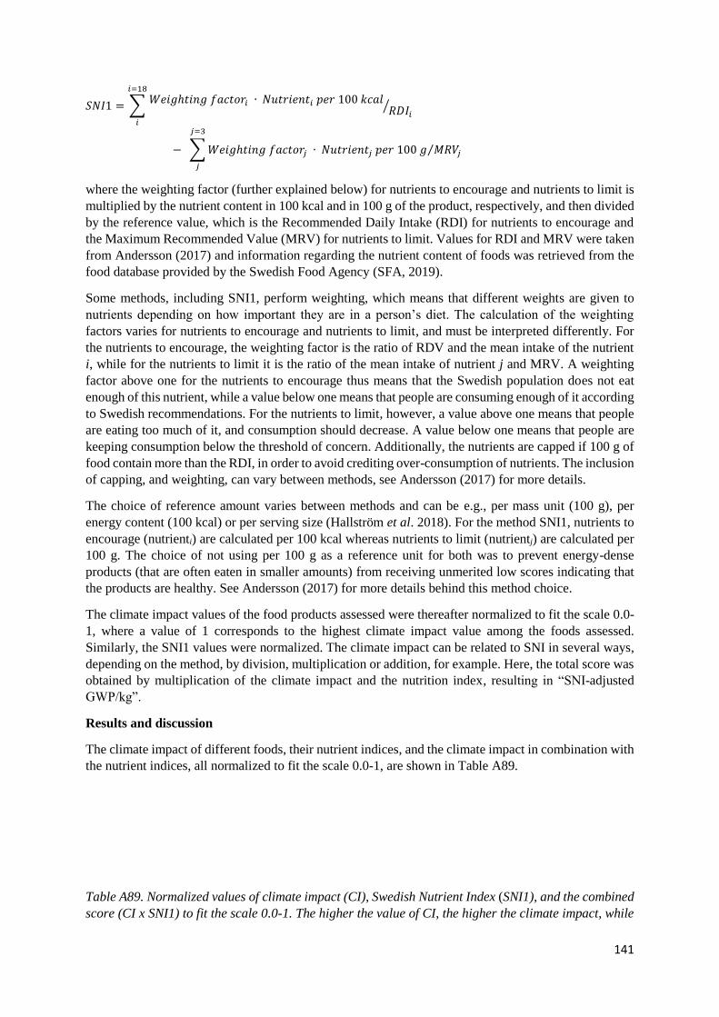
141

𝑆𝑁𝐼1 = ∑𝑊𝑒𝑖𝑔ℎ𝑡𝑖𝑛𝑔 𝑓𝑎𝑐𝑡𝑜𝑟𝑖 ∙ 𝑁𝑢𝑡𝑟𝑖𝑒𝑛𝑡𝑖 𝑝𝑒𝑟 100 𝑘𝑐𝑎𝑙

𝑅𝐷𝐼𝑖⁄

𝑖=18

𝑖

− ∑ 𝑊𝑒𝑖𝑔ℎ𝑡𝑖𝑛𝑔 𝑓𝑎𝑐𝑡𝑜𝑟𝑗 ∙ 𝑁𝑢𝑡𝑟𝑖𝑒𝑛𝑡𝑗 𝑝𝑒𝑟 100 𝑔 𝑀𝑅𝑉𝑗⁄

𝑗=3

𝑗

where the weighting factor (further explained below) for nutrients to encourage and nutrients to limit is

multiplied by the nutrient content in 100 kcal and in 100 g of the product, respectively, and then divided

by the reference value, which is the Recommended Daily Intake (RDI) for nutrients to encourage and

the Maximum Recommended Value (MRV) for nutrients to limit. Values for RDI and MRV were taken

from Andersson (2017) and information regarding the nutrient content of foods was retrieved from the

food database provided by the Swedish Food Agency (SFA, 2019).

Some methods, including SNI1, perform weighting, which means that different weights are given to

nutrients depending on how important they are in a person’s diet. The calculation of the weighting

factors varies for nutrients to encourage and nutrients to limit, and must be interpreted differently. For

the nutrients to encourage, the weighting factor is the ratio of RDV and the mean intake of the nutrient

i, while for the nutrients to limit it is the ratio of the mean intake of nutrient j and MRV. A weighting

factor above one for the nutrients to encourage thus means that the Swedish population does not eat

enough of this nutrient, while a value below one means that people are consuming enough of it according

to Swedish recommendations. For the nutrients to limit, however, a value above one means that people

are eating too much of it, and consumption should decrease. A value below one means that people are

keeping consumption below the threshold of concern. Additionally, the nutrients are capped if 100 g of

food contain more than the RDI, in order to avoid crediting over-consumption of nutrients. The inclusion

of capping, and weighting, can vary between methods, see Andersson (2017) for more details.

The choice of reference amount varies between methods and can be e.g., per mass unit (100 g), per

energy content (100 kcal) or per serving size (Hallström et al. 2018). For the method SNI1, nutrients to

encourage (nutrienti) are calculated per 100 kcal whereas nutrients to limit (nutrientj) are calculated per

100 g. The choice of not using per 100 g as a reference unit for both was to prevent energy-dense

products (that are often eaten in smaller amounts) from receiving unmerited low scores indicating that

the products are healthy. See Andersson (2017) for more details behind this method choice.

The climate impact values of the food products assessed were thereafter normalized to fit the scale 0.0-

1, where a value of 1 corresponds to the highest climate impact value among the foods assessed.

Similarly, the SNI1 values were normalized. The climate impact can be related to SNI in several ways,

depending on the method, by division, multiplication or addition, for example. Here, the total score was

obtained by multiplication of the climate impact and the nutrition index, resulting in “SNI-adjusted

GWP/kg”.

Results and discussion

The climate impact of different foods, their nutrient indices, and the climate impact in combination with

the nutrient indices, all normalized to fit the scale 0.0-1, are shown in Table A89.

Table A89. Normalized values of climate impact (CI), Swedish Nutrient Index (SNI1), and the combined

score (CI x SNI1) to fit the scale 0.0-1. The higher the value of CI, the higher the climate impact, while

142

a low value of SNI1 means that the food is healthy according to the SNI1 index. A high value of the

combined value (CI x SNI1) thus means that the product has a high carbon footprint among the foods

assessed or is less healthy according to Swedish nutritional recommendations

Product Climate

impact (kg

CO2e/kg)

Climate

norm.

SNI

norm.

CI x

SNI

Peas 0.8 0.2 0.50 0.12

Chickpeas canned 1.7 0.4 0.67 0.35

Almonds 3.8 1.0 0.84 0.96

Walnuts 3.3 0.9 1.00 1.00

Quorn 2.2 0.6 0.45 0.30

Banana 1.5 0.4 0.80 0.36

Apple 0.5 0.1 0.88 0.13

Tomato 2.3 0.6 0.31 0.22

Cucumber 2.3 0.6 0.40 0.28

Avocado 1.6 0.4 0.82 0.40

Asparagus 2.1 0.6 0.10 0.06

Celery 0.6 0.2 0.18 0.03

Broccoli 1.3 0.3 0.10 0.04

Blueberries 0.9 0.2 0.75 0.20

Strawberries 1.5 0.4 0.36 0.16

Quinoa 0.9 0.2 0.75 0.20

Wheat 0.6 0.2 0.95 0.17

Rice 2.0 0.5 0.95 0.57

Potato 0.4 0.1 0.71 0.09

As the results in Table A89 show, certain foodstuffs are significantly affected when including the

nutritional index of the products. Products that had the highest impact on the climate of the food

examined did not necessarily have the greatest impact when their nutrition index was included. For

example, the normalized value of the mean climate impact for asparagus received one of the highest

scores of the products assessed. This is because the impact from airfreight was taken into account.

However, the combined score (CI x SNI1, Table A89) was quite low when the nutrient index was taken

into account. This is because asparagus is high in nutrients such as vitamin A, vitamin C, and folate

which, despite the higher environmental impact, resulted in a low value when the environmental impact

was combined with the nutrition index.

Almonds and walnuts have a higher climate impact than fruits, for example. Nuts contain many nutrients

that are considered healthy for the human body. However, nuts are also quite high in saturated fat, which

gives an adverse effect on the total score. Furthermore, the weighting factor for saturated fat is >1,

indicating that the mean intake of saturated fat in Sweden is greater than recommended, which also

affects the result. In addition, nuts are energy-dense, which means that nuts will be heavily affected by

using 100 kcal instead of 100 g as a reference unit for the nutrients to encourage (nutrienti). This, together

with the earlier reasoning, explains why the total score (CI x SNI1) for nuts is relatively high compared

with that for other products such as vegetables.

The mean climate impact for tomato and cucumber is higher than for other vegetables such as avocado

and celery. This is because the impact from greenhouse cultivation is accounted for, which has a

relatively large impact on the average climate impact for these products. When the climate impact of

these foods was combined with their nutrition index, the combined score was relatively low, which

indicates that cucumber and tomato are nutritious and at the same time have a relatively low climate

143

impact. The same applies for broccoli, which thanks to its content of vitamin A, vitamin C, folate, iron,

calcium, potassium, etc. received a low score when the climate impact was combined with the nutrient

index. Additionally, the nutrients to limit are low for broccoli compared with the nutrients to encourage

(sodium, saturated fat and sugar), which contributed to the low combined score. Avocado did not get a

remarkably low score when the nutrition index was applied, which could be due to the amount of

saturated fat. The weighting factor for saturated fat shows that Swedes generally eat too much.

The only nutrient to limit that is significant for fruits is sugar. This is probably the main reason why

banana, which despite its health benefits (high in vitamin C, potassium, etc.) did not receive a lower

score when its nutrition index was included. Unlike salt and saturated fat, Swedes eat within

recommended limit when it comes to sugar. If this were not the case, however, the total score would

have been even higher for sugar-rich fruits. Berries such as strawberries contain low amounts of sugar.

They are also high in nutrients to encourage, such as folate, which is beneficial for the total score since

the weighting factor shows that Swedes eat too little folate. This contributed to the lower score obtained

for strawberries when the nutrient index was applied.

Potatoes had the lowest climate impact and one of the lowest combined impact values when the nutrition

index was taken into account. This is because potatoes have a low climate impact to begin with, 0.4 kg

CO2e per kg, and contain many of the nutrients considered healthy. In addition, the less healthy nutrients

that should be eaten in small amounts are not as significant in comparison with the beneficial nutrients.

Other nutrient indices

The method used in this report is only one among many existing methods to calculate nutrient index for

food. Other methods include different method choices, which affect the final score in different ways. To

address this, five additional methods were chosen for evaluation. First, three variations of SNI were

chosen, here called SNI2, SNI3, and SNI4. Second, NRF9 and NRF9.3 (Nutrient-Rich Food index) were

chosen for further evaluation. These methods, as well as SNI1, are based on existing nutrient profiling

methods, but are adapted with respect to food consumption, requirements, and recommendations for the

Swedish population. All 18 nutrients in SNI1 are included in SNI2, SNI3, and SNI4, but they vary in

their choice of reference amount (per 100 g or 100 kcal), and also if they are divided by the number of

nutrients included or not, see the following equations:

𝑆𝑁𝐼2 = ∑ 𝑊𝑒𝑖𝑔ℎ𝑡𝑖𝑛𝑔 𝑓𝑎𝑐𝑡𝑜𝑟𝑖 ∙ 𝑁𝑢𝑡𝑟𝑖𝑒𝑛𝑡𝑖 𝑝𝑒𝑟 100 𝑘𝑐𝑎𝑙 𝑅𝐷𝐼𝑖 18⁄⁄

𝑖=18

𝑖

− ∑ 𝑊𝑒𝑖𝑔ℎ𝑡𝑖𝑛𝑔 𝑓𝑎𝑐𝑡𝑜𝑟𝑗 ∙ 𝑁𝑢𝑡𝑟𝑖𝑒𝑛𝑡𝑗 𝑝𝑒𝑟 100 𝑔 𝑀𝑅𝑉𝑗⁄ 3⁄

𝑗=3

𝑗

𝑆𝑁𝐼3 = ∑ 𝑊𝑒𝑖𝑔ℎ𝑡𝑖𝑛𝑔 𝑓𝑎𝑐𝑡𝑜𝑟𝑖 ∙ 𝑁𝑢𝑡𝑟𝑖𝑒𝑛𝑡𝑖 𝑝𝑒𝑟 100 𝑔 𝑅𝐷𝐼𝑖⁄

𝑖=18

𝑖

− ∑ 𝑊𝑒𝑖𝑔ℎ𝑡𝑖𝑛𝑔 𝑓𝑎𝑐𝑡𝑜𝑟𝑗 ∙ 𝑁𝑢𝑡𝑟𝑖𝑒𝑛𝑡𝑗 𝑝𝑒𝑟 100 𝑔 𝑀𝑅𝑉𝑗⁄

𝑗=3

𝑗

𝑆𝑁𝐼4 = ∑ 𝑊𝑒𝑖𝑔ℎ𝑡𝑖𝑛𝑔 𝑓𝑎𝑐𝑡𝑜𝑟𝑖 ∙ 𝑁𝑢𝑡𝑟𝑖𝑒𝑛𝑡𝑖 𝑝𝑒𝑟 100 𝑔 𝑅𝐷𝐼𝑖 18⁄⁄

𝑖=18

𝑖

− ∑ 𝑊𝑒𝑖𝑔ℎ𝑡𝑖𝑛𝑔 𝑓𝑎𝑐𝑡𝑜𝑟𝑗 ∙ 𝑁𝑢𝑡𝑟𝑖𝑒𝑛𝑡𝑗 𝑝𝑒𝑟 100 𝑔 𝑀𝑅𝑉𝑗⁄ 3⁄

𝑗=3

𝑗

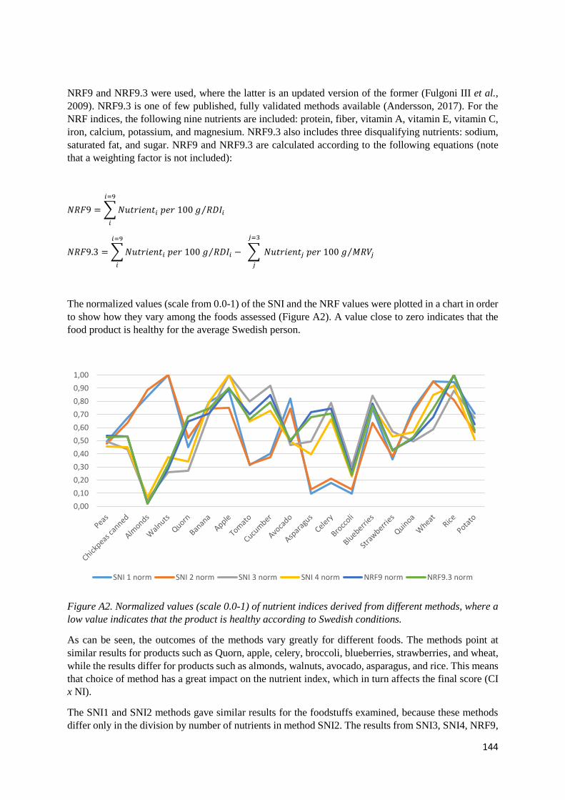
144

NRF9 and NRF9.3 were used, where the latter is an updated version of the former (Fulgoni III et al.,

2009). NRF9.3 is one of few published, fully validated methods available (Andersson, 2017). For the

NRF indices, the following nine nutrients are included: protein, fiber, vitamin A, vitamin E, vitamin C,

iron, calcium, potassium, and magnesium. NRF9.3 also includes three disqualifying nutrients: sodium,

saturated fat, and sugar. NRF9 and NRF9.3 are calculated according to the following equations (note

that a weighting factor is not included):

𝑁𝑅𝐹9 = ∑ 𝑁𝑢𝑡𝑟𝑖𝑒𝑛𝑡𝑖 𝑝𝑒𝑟 100 𝑔 𝑅𝐷𝐼𝑖⁄

𝑖=9

𝑖

𝑁𝑅𝐹9.3 = ∑ 𝑁𝑢𝑡𝑟𝑖𝑒𝑛𝑡𝑖 𝑝𝑒𝑟 100 𝑔 𝑅𝐷𝐼𝑖⁄ − ∑ 𝑁𝑢𝑡𝑟𝑖𝑒𝑛𝑡𝑗 𝑝𝑒𝑟 100 𝑔 𝑀𝑅𝑉𝑗⁄

𝑗=3

𝑗

𝑖=9

𝑖

The normalized values (scale from 0.0-1) of the SNI and the NRF values were plotted in a chart in order

to show how they vary among the foods assessed (Figure A2). A value close to zero indicates that the

food product is healthy for the average Swedish person.

Figure A2. Normalized values (scale 0.0-1) of nutrient indices derived from different methods, where a

low value indicates that the product is healthy according to Swedish conditions.

As can be seen, the outcomes of the methods vary greatly for different foods. The methods point at

similar results for products such as Quorn, apple, celery, broccoli, blueberries, strawberries, and wheat,

while the results differ for products such as almonds, walnuts, avocado, asparagus, and rice. This means

that choice of method has a great impact on the nutrient index, which in turn affects the final score (CI

x NI).

The SNI1 and SNI2 methods gave similar results for the foodstuffs examined, because these methods

differ only in the division by number of nutrients in method SNI2. The results from SNI3, SNI4, NRF9,

0,00

0,10

0,20

0,30

0,40

0,50

0,60

0,70

0,80

0,90

1,00

SNI 1 norm SNI 2 norm SNI 3 norm SNI 4 norm NRF9 norm NRF9.3 norm

145

and NRF9.3 vary among the food products assessed, but follow the same pattern in general (Figure A2).

This is because the calculations in these methods are based on the same reference value (per 100 g).

However, the methods account for different numbers of nutrients and some do not include weighting,

which may be a reason for the minor variations in the results.

Using SNI1 and SNI2 appears to be less favorable for energy-dense products such as nuts, avocado, and

rice, while using SNI3, SNI4, NRF9, or NRF9.3 seems to be more favorable for these products.

Similarly, low-energy fruit and vegetables seem to be favored by the SNI1 and SNI2 methods, while the

other methods seem less favorable. One likely reason behind the various results among the methods

assessed is the choice of reference unit (100 g or 100 kcal, or a mix of them), which seems to influence

the result greatly.

Limitations

Designing a nutrition index means several subjective choices that affect the end result. For example, a

decision is needed on how many and which nutrients to include. This is challenging, as a healthy food

products can vary depending on the individual; a product that is healthy for one person is not necessarily

healthy for another. A decision is also needed concerning the unit on which the calculations on nutrients

to encourage/limit should be based, e.g., grams, kcal, or portion size. Furthermore, a decision is needed

on whether weighting should be included or not. It is important to emphasize that weighting factors need

to be updated from time to time because people’s eating habits change, which will affect the factors. If

weighting is not applied, equal weight will be given to the final score from all the nutrients included.

The combination of the climate impact and nutrition index can also be obtained in different ways, which

will affect the total score.

Conclusions

Designing a nutrient index involves many choices, which may limit the credibility of the results. Despite

the limitations in the design of nutrition index, it can nevertheless be used to broaden the knowledge and

understanding of the sustainability of foods. The combined measure can thus be useful and contribute

an understanding of how climate footprint relates to nutrition, but should be interpreted and applied with

caution as the method involves several subjective choices.

146

Appendix A5. Food losses, waste, and conversion factors

Table A90. Factors for calculating losses in post-harvest handling and storage, processing and packing,

and distribution: supermarket retail (Gustavsson et al., 2011) Postharvest handling and

storage

Processing and

packing

Distribution:

supermarket retail

Europe incl. Russia Cereals

4%

10.50%

Roots and tubers 9% 15% 7%

Oilseeds and pulses 1% 5% 1%

Fruit and vegetables 5% 2% 10%

North America and Oceania

Cereals 2% 10.50% 2%

Roots and tubers 10% 15% 7%

Oilseeds and pulses 0% 5% 1%

Fruit and vegetables 4% 2% 12%

Industrialized Asia

Cereals 10% 10.50% 2%

Roots and tubers 7% 15% 9%

Oilseeds and pulses 3% 5% 1%

Fruit and vegetables 8% 2% 8%

Sub-Saharan Africa

Cereals 8% 3.50% 2%

Roots and tubers 18% 15% 5%

Oilseeds and pulses 8% 8% 2%

Fruit and vegetables 9% 25% 17%

North Africa, West and

Central Asia

Cereals 8% 9% 4%

Roots and tubers 10% 12% 4%

Oilseeds and pulses 6% 8% 2%

Fruit and vegetables 10% 20% 15%

South and Southeast Asia

Cereals 7% 3.50% 2%

Roots and tubers 19% 10% 11%

Oilseeds and pulses 12% 8% 2%

Fruit and vegetables 9% 25% 10%

Latin America

Cereals 4% 9% 4%

Roots and tubers 14% 12% 3%

Oilseeds and pulses 3% 8% 2%

Fruit and vegetables 10% 20% 12%

AVERAGE Postharvest handling and

storage

Processing and

packing

Distribution: supermarket

retail

Cereals 6% 8% 3%

147

Roots and tubers 12% 13% 7%

Oilseeds and pulses 5% 7% 2%

Fruit and vegetables 8% 14% 12%

Conversion factors for nuts from in-shell to shelled

Table A91. Conversion factors for converting in-shell products to shelled products, showing the fraction

of edible nut in 1 kg nuts in shell

Product Factor Reference

Almonds 0.59 Bartzas et al. (2017)

Cashew nuts 0.25 FAO (1994)

Hazelnuts 0.50 FAO (1994)

Peanuts 0.83 Mccarty et al. (2012)

Pistachios 0.50 Marvinney et al. (2014)

Walnuts 0.53 FAO (1994)

Conversion factors for carbohydrate sources

Table A92. Conversion factors for converting dried carbohydrate sources to edible products Product Factor Reference

Soft whole grain bread 2.0 RAC

Bread rye 1.8 RAC

White bread

1.8 RAC

Pasta

2.1 Bognár (2002)

Wheat whole boiled 1.8 Bognár (2002)

Average for

common grainsa

1.9

Rice

3.0 Bognár (2002)

Millet

2.4 Bognár (2002)

Quinoa

3.4 Bognár (2002) aUsed for barley, corn, oat, pasta, rye, sorghum and wheat.

Conversion factors for protein sources

Table A93. Conversion factors for converting dried grain legumes to edible products Product Factor Reference

Beans and peasa

2.5 Bognár (2002)

Lentils 2.3 SFA (2019)b

Soybeans 3.1 SFA (2019)b

Chickpeas 2.5 aUsed for dried beans, kidney beans, faba beans, and dried peas. bCalculated based on protein content in dried and edible product.

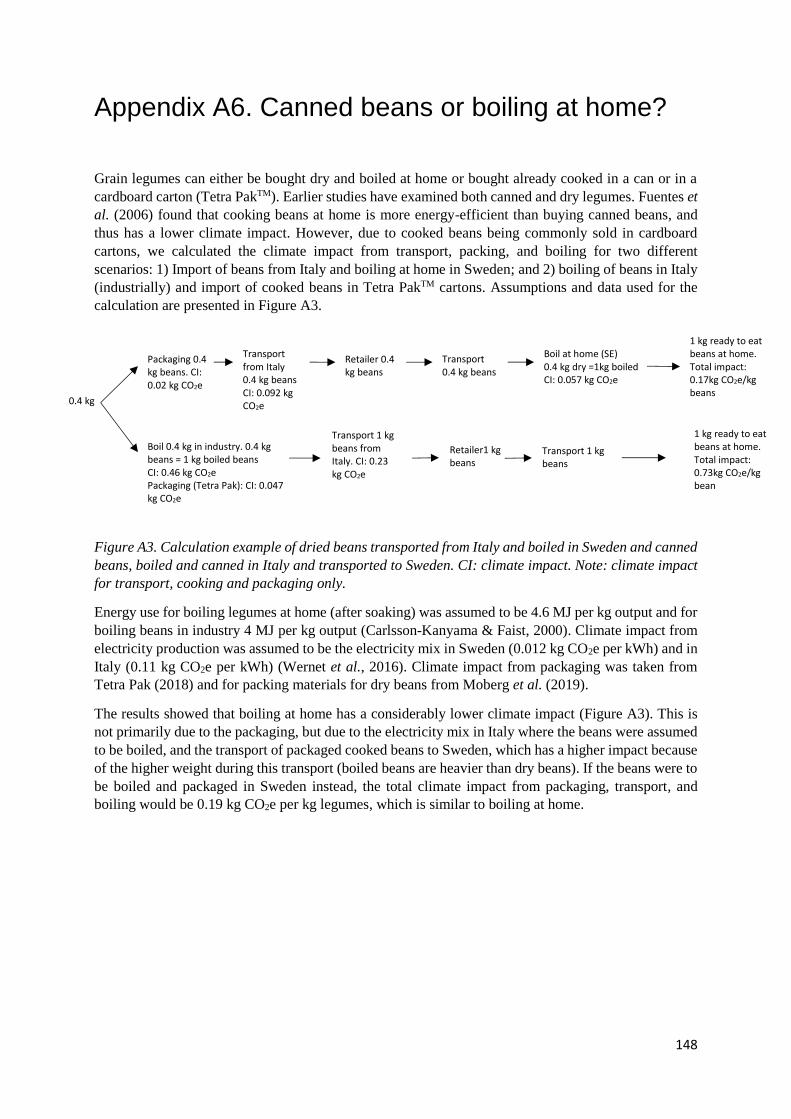
148

Appendix A6. Canned beans or boiling at home?

Grain legumes can either be bought dry and boiled at home or bought already cooked in a can or in a

cardboard carton (Tetra PakTM). Earlier studies have examined both canned and dry legumes. Fuentes et

al. (2006) found that cooking beans at home is more energy-efficient than buying canned beans, and

thus has a lower climate impact. However, due to cooked beans being commonly sold in cardboard

cartons, we calculated the climate impact from transport, packing, and boiling for two different

scenarios: 1) Import of beans from Italy and boiling at home in Sweden; and 2) boiling of beans in Italy

(industrially) and import of cooked beans in Tetra PakTM cartons. Assumptions and data used for the

calculation are presented in Figure A3.

Figure A3. Calculation example of dried beans transported from Italy and boiled in Sweden and canned

beans, boiled and canned in Italy and transported to Sweden. CI: climate impact. Note: climate impact

for transport, cooking and packaging only.

Energy use for boiling legumes at home (after soaking) was assumed to be 4.6 MJ per kg output and for

boiling beans in industry 4 MJ per kg output (Carlsson-Kanyama & Faist, 2000). Climate impact from

electricity production was assumed to be the electricity mix in Sweden (0.012 kg CO2e per kWh) and in

Italy (0.11 kg CO2e per kWh) (Wernet et al., 2016). Climate impact from packaging was taken from

Tetra Pak (2018) and for packing materials for dry beans from Moberg et al. (2019).

The results showed that boiling at home has a considerably lower climate impact (Figure A3). This is

not primarily due to the packaging, but due to the electricity mix in Italy where the beans were assumed

to be boiled, and the transport of packaged cooked beans to Sweden, which has a higher impact because

of the higher weight during this transport (boiled beans are heavier than dry beans). If the beans were to

be boiled and packaged in Sweden instead, the total climate impact from packaging, transport, and

boiling would be 0.19 kg CO2e per kg legumes, which is similar to boiling at home.

0.4 kg

Packaging 0.4 kg beans. CI: 0.02 kg CO2e

Transport from Italy 0.4 kg beans CI: 0.092 kg CO2e

Retailer 0.4 kg beans

Transport 0.4 kg beans

Boil at home (SE) 0.4 kg dry =1kg boiled CI: 0.057 kg CO2e

Boil 0.4 kg in industry. 0.4 kg beans = 1 kg boiled beans CI: 0.46 kg CO2e Packaging (Tetra Pak): CI: 0.047 kg CO2e

Transport 1 kg beans from Italy. CI: 0.23 kg CO2e

Transport 1 kg beans

Retailer1 kg beans

1 kg ready to eat beans at home. Total impact: 0.73kg CO2e/kg bean

1 kg ready to eat beans at home. Total impact: 0.17kg CO2e/kg beans

149

Appendix A7. Pesticide use results for individual products

Table A94. Pesticide for individual products in kg active substance (AS) per hectare and g AS per kg

product (OE: outside Europe, ND: no data) Product Country Comments

pesticides

Pesticide

use (kg

AS/ha)

Pesticide

use (g

AS/kg)

Total

pesticide for

combined

products

References

Peas fresh Belgium Other arable crops 0.25 0.04 EUROSTAT (2007)

The Netherlands No data for other

arable crops ND ND EUROSTAT

(2007)

France (largest trade surplus)

Other arable crops 0.10 0.01 EUROSTAT (2007)

World average OE ND ND

Peas canned Belgium Other arable crops 0.25 0.04 EUROSTAT

(2007) Italy No data for other

arable crops ND ND EUROSTAT

(2007)

Germany Other arable crops 0.13 0.02 EUROSTAT

(2007)

France (largest

trade surplus)

Other arable crops 0.10 0.01 EUROSTAT

(2007)

World average OE ND ND

Peas fresh (frozen)

Sweden

Sweden Green peas 1.10 0.25 SBA (2018)

Peas dried Denmark Other arable crops 0.08 0.01 EUROSTAT

(2007)

The Netherlands No data for other

arable crops

ND ND

Germany Other arable crops 0.13 0.02 EUROSTAT (2007)

Canada (largest

trade surplus)

OE ND ND

World average OE ND ND

Sweden Peas dried 0.99 0.13 SBA (2018)

Beans dried Turkey OE ND ND

The Netherlands No data for other

arable crops

ND ND

Myanmar

(largest trade

surplus)

OE ND ND

Argentina (extra

country)

OE ND ND

Poland (extra

country)

No data for other

arable crops

ND ND

Canada OE ND ND

China OE ND ND

World average OE ND ND

Sweden Data for faba

beans

1.01 0.25 SBA (2018)

Faba beans dried Egypt OE ND ND

Lebanon OE ND ND

Turkey OE ND ND

Germany Other arable crops 0.13 0.01 EUROSTAT

(2007)

Australia

(largest trade

surplus)

OE ND ND

UK (extra

country)

Other arable crops 2.60 0.29 EUROSTAT

(2007)

France (extra country)

Other arable crops 0.10 0.01 EUROSTAT (2007)

150

World average OE ND ND

Sweden Faba beans 1.01 0.12 SBA (2018)

Beans canned Italy No data for other arable crops

ND ND

Myanmar

(largest trade surplus)

OE ND ND

World average OE ND ND

Sweden Data for faba

beans

1.01 0.25 SBA (2018)

Chickpeas dried Turkey OE ND ND

Italy No data for other arable crops

ND ND

Australia

(largest trade surplus)

OE ND ND

World average OE ND ND

Lentils dried Turkey OE ND ND

UK No data for other

arable crops

ND ND

Canada (largest

trade surplus)

OE ND ND

World average OE ND ND

Sweden Data for faba

beans

1.01 0.32 SBA (2018)

Soybeans dried Italy Data for oil crops 0.34 0.03 EUROSTAT

(2007)

USA (largest trade surplus)

OE ND ND

World average OE ND ND

Soy-based

products

USA (soybeans) ND ND

Tofu/tempeh USA ND ND

Faba beans or peas

(tofu/tempeh)

Sweden 1.01 0.24 SBA (2018)

Quorn UK Cereals (wheat) 3.18 0.35 EUROSTAT

(2007)

Pea-protein based Germany Data for other

arable crops

0.13 0.06 EUROSTAT

(2007)

Almonds USA OE ND ND

Australia OE ND ND

Spain No data ND ND

USA (largest

trade surplus)

OE ND ND

Chile (extra

country)

OE ND ND

Italy (extra European

country)

No data ND ND

World average OE ND ND

Cashew nuts Vietnam (largest trade surplus)

OE ND ND

Extra India OE ND ND

Brazil (extra

country)

OE ND ND

World average OE ND ND

Chestnuts China (largest trade surplus)

OE ND ND

World average OE ND ND

Coconut Philippines

(largest trade

surplus)

OE ND ND

Indonesia (extra

country)

OE ND ND

Sri Lanka (extra country)

OE ND ND

World average OE ND ND

Hazelnuts Italy No data ND ND

151

Turkey (largest

trade surplus)

OE ND ND

World average OE ND ND

Peanuts Argentina OE ND ND

China OE ND ND

India (largest

trade surplus)

OE ND ND

World average OE ND ND

Pistachios USA (largest trade surplus)

OE ND ND

Iran (extra

country)

OE ND ND

Turkey (extra

country)

No data ND ND

Greece (extra country)

No data ND ND

World average OE ND ND

Walnuts USA (largest

trade surplus)

OE ND ND

Ukraine (extra

country)

No data ND ND

Mexico (extra country)

OE ND ND

Republic of

Moldova (extra country)

No data ND ND

World average OE ND ND

Sesame seeds India OE ND ND

Guatemala OE ND ND

Ethiopia (largest

trade surplus)

OE ND ND

World average OE ND ND

Linseeds Denmark Oilseeds 0.26 0.92 EUROSTAT

(2007)

Canada OE ND ND

The Netherlands Oil crops 2.84 3.39 EUROSTAT

(2007)

World average OE ND ND

Sweden Oil crops 0.48 0.28 EUROSTAT

(2007)

Sunflower seeds Bulgaria No data ND ND

Russia OE ND ND

Romania (largest trade

surplus)

no data ND ND

World average OE ND ND

Barley Denmark Cereals 0.92 0.10 EUROSTAT (2007)

Finland Cereals 0.56 0.10 EUROSTAT

(2007)

UK & Northern

Ireland

Cereals 3.18 0.33 EUROSTAT

(2007)

France (largest trade surplus)

Cereals 2.58 0.24 EUROSTAT (2007)

World average OE ND ND

Sweden Barley (average

winter and spring)

0.50 0.06 SBA (2018)

Maize France Maize 2.16 0.15 EUROSTAT

(2007)

Poland Maize 1.10 0.10 EUROSTAT (2007)

South Africa

(largest trade surplus)

OE ND ND

Brazil (extra

country)

OE ND ND

Argentina (extra

country)

OE ND ND

World average OE ND ND

152

Millet India (largest

trade surplus)

OE ND ND

World average OE ND ND

Oats Denmark Cereals 0.92 0.11 EUROSTAT (2007)

Finland Cereals 0.56 0.10 EUROSTAT

(2007)

Canada OE ND ND

World average OE ND ND

Sweden Oats 0.37 0.05 SBA (2018)

Pasta Denmark Cereals 0.92 0.09 EUROSTAT

(2007)

Finland Cereals 0.56 0.10 EUROSTAT

(2007)

Germany Cereals 2.16 0.19 EUROSTAT (2007)

Turkey (largest trade surplus)

OE ND ND

World average OE ND ND

Italy cereals 0.48 0.08 EUROSTAT

(2007)

Sweden Wheat (average spring and winter)

0.50 0.06 SBA (2018)

Quinoa Peru OE ND ND

Bolivia OE ND ND

World average OE ND ND

Sweden Assumption, no

accepted value for

quinoa in Sweden

0.00 0.00

Rice India OE ND ND

Italy Cereals 0.48 0.05 EUROSTAT

(2007)

Thailand OE ND ND

India (largest

trade surplus)

OE ND ND

World average OE ND ND

Rye Denmark Cereals 0.92 0.09 EUROSTAT (2007)

Finland Cereals 0.56 0.12 EUROSTAT

(2007)

Poland Cereals 0.70 0.15 EUROSTAT

(2007)

Germany Cereals 2.16 0.23 EUROSTAT (2007)

World average OE ND ND

Sweden Rye 1.16 0.12 SBA (2018)

Sorghum USA (largest

trade surplus)

OE ND ND

World average OE ND ND

Wheat Denmark Cereals 0.92 0.08 EUROSTAT (2007)

Finland Cereals 0.56 0.09 EUROSTAT

(2007)

Germany Cereals 2.16 0.16 EUROSTAT

(2007)

Turkey (largest trade surplus)

OE ND ND

UK (extra for

Quorn)

Cereals 3.18 0.48 EUROSTAT

(2007)

World average OE ND ND

Sweden Wheat (average

spring and winter)

0.50 0.05 SBA (2018)

Beetroot The Netherlands Vegetables 2.74 0.10 EUROSTAT (2007)

Denmark Vegetables 14.36 0.53 EUROSTAT

(2007)

Germany Vegetables 2.16 0.08 EUROSTAT

(2007)

Not available in FAOSTAT

ND ND

153

World average OE ND ND

Sweden Vegetables 2.20 0.08 SBA (2018)

Carrots Italy Vegetables 7.04 0.21 EUROSTAT (2007)

The Netherlands Vegetables 2.74 0.06 EUROSTAT

(2007)

China (largest

trade surplus)

OE ND ND

World average OE ND ND

Sweden carrots 15.60 0.36 SBA (2018)

Potatoes Denmark Potatoes 6.94 0.23 EUROSTAT

(2007)

Finland Potatoes 3.48 0.18 EUROSTAT

(2007)

France (largest trade surplus)

Potatoes 17.26 0.54 EUROSTAT (2007)

World average OE ND ND

Sweden Potatoes 2.91 0.12 SBA (2018)

Swede (rutabaga) Sweden Vegetables 2.20 0.10 SBA (2018)

Sweet potato USA (largest

trade surplus)

OE ND ND

World average OE ND ND

Parsnip Not available in import statistics

ND ND

Sweden Vegetables 2.20 0.12 SBA (2018)

Jerusalem

artichoke

Sweden Vegetables 2.20 0.22 SBA (2018)

Almond milk 1 USA (almonds) OE ND ND ND

Brazil (sugar) OE ND ND ND

Almond milk 2 Australia

(almonds)

OE ND ND ND

Brazil (sugar) OE ND ND ND

Almond milk 3 Spain (almonds) No data ND ND ND

Brazil (sugar) OE ND ND ND

Almond milk 4 World average (almonds)

OE ND ND ND

Brazil (largest

producer) (sugar)

OE ND ND ND

Soy milk 1

(sweetened)

Italy (soybeans) Oil seeds 0.34 0.01 0.007131 EUROSTAT

(2007)

Brazil (sugar) OE ND ND

France (corn) Maize 2.16 0.00 EUROSTAT (2007)

Soy milk 2

(sweetened)

USA (soybeans) OE ND ND 8.5E-05

Brazil (sugar) OE ND ND

France (corn) Maize 2.16 0.00 EUROSTAT

(2007)

Soy milk 3

(sweetened)

World average (soymilk)

OE ND ND ND

Brazil (sugar) OE ND ND ND

World average

(corn)

OE ND ND ND

Oat milk 1 Sweden (oats) Oat 0.37 0.02 0.022187 SBA (2018)

Sweden (rapeseed oil)

Average winter and spring rape

0.60 0.00

Oat milk 2 World average

(oats)

OE ND ND ND

World average

(rapeseed oil)

OE ND ND

Oat cream 1 Sweden (oats) Oat 0.37 0.02 0.046366 SBA (2018)

Sweden (rapeseed oil)

Average winter and spring rape

0.60 0.03

Oat cream 2 World average

(oats)

OE ND ND ND

World average

(rapeseed oil)

OE ND ND

154

Coconut milk 1 Philippines OE ND ND ND

Coconut milk 2 Indonesia (extra

country)

OE ND ND ND

Coconut milk 3 Sri Lanka (extra country)

OE ND ND ND

Coconut milk 4 World average OE ND ND ND

Apples Italy Fruit trees 14.64 0.42 EUROSTAT

(2007)

Poland (largest trade surplus)

Fruit trees 2.38 0.17 EUROSTAT (2007)

France (extra

country)

Fruit trees 16.38 0.49 EUROSTAT

(2007)

World average OE ND ND

Sweden Apples 4.22 0.28 SBA (2018)

Apricots France Fruit trees 16.38 1.65 EUROSTAT (2007)

Italy Fruit trees 14.64 1.45 EUROSTAT (2007)

Spain Fruit trees 2.76 0.45 EUROSTAT

(2007)

Germany Fruit trees 16.20 4.25 EUROSTAT

(2007)

Spain (largest exporter)

Fruit trees 2.76 0.45 EUROSTAT (2007)

Turkey (extra

country)

No data ND ND

Uzbekistan

(extra country)

OE ND ND

Armenia (extra country)

OE ND ND

World average OE ND ND

Bananas Costa Rica OE ND ND

Dominican

Republic

OE ND ND

Ecuador (largest exporter)

OE ND ND

World average OE ND ND

Cherries Denmark (Chile) OE ND ND

The Netherlands Fruit trees 16.78 42.06 EUROSTAT

(2007)

Turkey OE ND ND

Germany Fruit trees 15.80 3.51 EUROSTAT

(2007)

Chile (largest

exporter)

OE ND ND

USA (extra country)

OE ND ND

Spain (extra country)

Fruit trees 2.76 0.83 EUROSTAT (2007)

World average OE ND ND

Dates Iran OE ND ND

Saudi Arabia OE ND ND

Iraq (largest trade surplus)

OE ND ND

Pakistan (extra

country)

OE ND ND

Tunisia (extra

country)

OE ND ND

World average OE ND ND

Grapefruit and

pomelo

South Africa (largest trade

surplus)

OE ND ND

World average OE ND ND

Grapes Chile (largest

exporter)

OE ND ND

Greece Grapes/vines 44.58 4.77 EUROSTAT

(2007)

Italy Grapes/vines 32.24 3.42 EUROSTAT (2007)

155

The Netherlands

(Chile)

OE ND ND

Spain Grapes/vines 10.48 1.90 EUROSTAT (2007)

World average OE ND ND

Guavas and mango Mexico (largest

exporter)

OE ND ND

India (extra

country)

OE ND ND

Thailand (extra country)

OE ND ND

World average OE ND ND

Kiwi fruit New Zealand

(largest trade surplus)

OE ND ND

Italy Fruit trees 14.64 0.87 EUROSTAT

(2007)

World average OE ND ND

Lemons and limes Mexico (largest trade surplus)

OE ND ND

Spain Citrus 8.40 0.43 EUROSTAT

(2007)

Turkey (extra

country)

No data ND ND

Argentina (extra country)

OE ND ND

World average OE ND ND

Melons Guatemala

(largest trade surplus)

OE ND ND

Spain Fruit and

vegetables total

8.38 0.31 EUROSTAT

(2007)

OE ND ND

Honduras (extra country)

OE ND ND

Turkey (extra

country)

No data ND ND

Greece (extra

country)

Fruits and

vegetables total

16.54 0.87 EUROSTAT

(2007)

World average OE ND ND

Sweden ND ND

Oranges Spain (largest

trade surplus)

Citrus 8.40 0.43 EUROSTAT

(2007)

South Africa

(extra country)

OE ND ND

Egypt (extra

country)

OE ND ND

Greece (extra

country)

Citrus 1.88 0.08 EUROSTAT

(2007)

World average OE ND ND

Papayas Mexico (largest

trade surplus)

OE ND ND

Thailand OE ND ND

World average OE ND ND

Peach Italy Fruit trees 14.64 0.91 EUROSTAT

(2007)

Germany Fruit trees 16.20 2.07 EUROSTAT

(2007)

Spain (largest trade surplus)

Fruit trees 2.76 0.18 EUROSTAT (2007)

World average OE ND ND EUROSTAT

(2007)

Pears Belgium Fruit trees 19.80 0.66 EUROSTAT

(2007)

The Netherlands Fruit trees 16.78 0.53 EUROSTAT (2007)

Argentina

(largest exporter)

OE ND ND

World average OE ND ND

Sweden Fruit 4.15 0.38 SBA (2018)

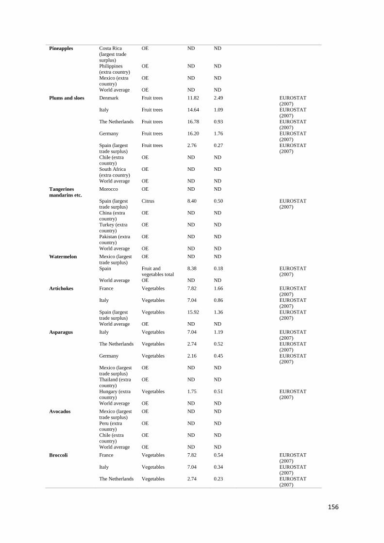
156

Pineapples Costa Rica

(largest trade

surplus)

OE ND ND

Philippines

(extra country)

OE ND ND

Mexico (extra country)

OE ND ND

World average OE ND ND

Plums and sloes Denmark Fruit trees 11.82 2.49 EUROSTAT

(2007)

Italy Fruit trees 14.64 1.09 EUROSTAT

(2007)

The Netherlands Fruit trees 16.78 0.93 EUROSTAT (2007)

Germany Fruit trees 16.20 1.76 EUROSTAT

(2007)

Spain (largest

trade surplus)

Fruit trees 2.76 0.27 EUROSTAT

(2007)

Chile (extra country)

OE ND ND

South Africa

(extra country)

OE ND ND

World average OE ND ND

Tangerines

mandarins etc.

Morocco OE ND ND

Spain (largest trade surplus)

Citrus 8.40 0.50 EUROSTAT (2007)

China (extra

country)

OE ND ND

Turkey (extra

country)

OE ND ND

Pakistan (extra country)

OE ND ND

World average OE ND ND

Watermelon Mexico (largest

trade surplus)

OE ND ND

Spain Fruit and vegetables total

8.38 0.18 EUROSTAT (2007)

World average OE ND ND

Artichokes France Vegetables 7.82 1.66 EUROSTAT

(2007)

Italy Vegetables 7.04 0.86 EUROSTAT

(2007)

Spain (largest trade surplus)

Vegetables 15.92 1.36 EUROSTAT (2007)

World average OE ND ND

Asparagus Italy Vegetables 7.04 1.19 EUROSTAT

(2007)

The Netherlands Vegetables 2.74 0.52 EUROSTAT

(2007)

Germany Vegetables 2.16 0.45 EUROSTAT (2007)

Mexico (largest

trade surplus)

OE ND ND

Thailand (extra

country)

OE ND ND

Hungary (extra country)

Vegetables 1.75 0.51 EUROSTAT (2007)

World average OE ND ND

Avocados Mexico (largest

trade surplus)

OE ND ND

Peru (extra country)

OE ND ND

Chile (extra

country)

OE ND ND

World average OE ND ND

Broccoli France Vegetables 7.82 0.54 EUROSTAT

(2007)

Italy Vegetables 7.04 0.34 EUROSTAT (2007)

The Netherlands Vegetables 2.74 0.23 EUROSTAT

(2007)

157

Spain (largest

trade surplus)

Vegetables 15.92 1.01 EUROSTAT

(2007)

World average OE ND ND

Sweden Vegetables 2.20 0.21 SBA (2018)

Cabbage Spain Vegetables 15.92 0.55 EUROSTAT

(2007)

Germany Vegetables 2.16 0.04 EUROSTAT

(2007)

China (largest trade surplus)

OE ND ND

World average OE ND ND

Sweden Vegetables 2.20 0.06 SBA (2018)

Capsicums/peppers The Netherlands Vegetables 2.74 0.01 EUROSTAT

(2007)

Spain Vegetables 15.92 0.32 EUROSTAT (2007)

Mexico (largest trade surplus)

OE ND ND

World average OE ND ND

Celery The Netherlands ND ND

Spain ND ND

Germany ND ND

USA (assumption)

ND ND

World average ND ND

Cucumbers The Netherlands Vegetables 2.74 0.00 EUROSTAT

(2007)

Spain Vegetables 15.92 0.22 EUROSTAT (2007)

Mexico (largest

trade surplus)

OE ND ND

World average OE ND ND

Sweden Vegetables 2.20 0.02 SBA (2018)

Eggplant The Netherlands Vegetables 2.74 0.01 EUROSTAT (2007)

Spain (largest

trade surplus)

Vegetables 15.92 0.30 EUROSTAT

(2007)

World average OE ND ND

Garlic The Netherlands Vegetables 2.74 0.00 EUROSTAT

(2007)

Spain Vegetables 15.92 2.01 EUROSTAT (2007)

China (largest

trade surplus)

OE ND ND

Argentina (extra

country)

OE ND ND

World average OE ND ND

Sweden ND ND

Beans fresh

(haricoverts)

Belgium Vegetables 6.84 0.60 EUROSTAT

(2007)

The Netherlands Vegetables 2.74 0.29 EUROSTAT

(2007)

Morocco (largest trade

surplus)

OE ND ND

Kenya (extra country)

OE ND ND

Peru (extra

country)

OE ND ND

World average OE ND ND

Ginger China (largest

trade surplus)

OE ND ND

World average OE ND ND

Lettuce Spain (largest

trade surplus)

Vegetables 15.92 0.68 EUROSTAT

(2007)

Germany Vegetables 2.16 0.10 EUROSTAT

(2007)

World average OE ND ND

Sweden Vegetables 2.20 0.13 SBA (2018)

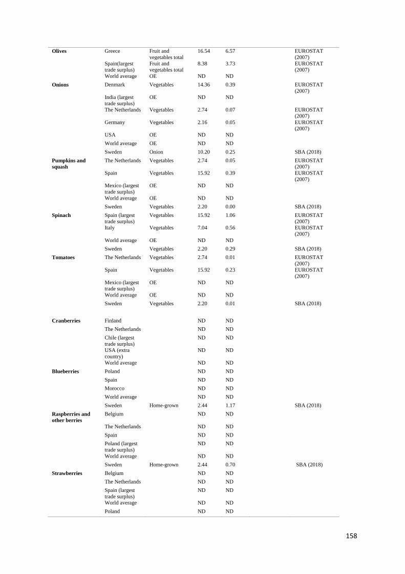
158

Olives Greece Fruit and

vegetables total

16.54 6.57 EUROSTAT

(2007)

Spain(largest trade surplus)

Fruit and vegetables total

8.38 3.73 EUROSTAT (2007)

World average OE ND ND

Onions Denmark Vegetables 14.36 0.39 EUROSTAT

(2007)

India (largest

trade surplus)

OE ND ND

The Netherlands Vegetables 2.74 0.07 EUROSTAT (2007)

Germany Vegetables 2.16 0.05 EUROSTAT

(2007)

USA OE ND ND

World average OE ND ND

Sweden Onion 10.20 0.25 SBA (2018)

Pumpkins and

squash

The Netherlands Vegetables 2.74 0.05 EUROSTAT (2007)

Spain Vegetables 15.92 0.39 EUROSTAT

(2007)

Mexico (largest

trade surplus)

OE ND ND

World average OE ND ND

Sweden Vegetables 2.20 0.00 SBA (2018)

Spinach Spain (largest

trade surplus)

Vegetables 15.92 1.06 EUROSTAT

(2007)

Italy Vegetables 7.04 0.56 EUROSTAT

(2007)

World average OE ND ND

Sweden Vegetables 2.20 0.29 SBA (2018)

Tomatoes The Netherlands Vegetables 2.74 0.01 EUROSTAT

(2007)

Spain Vegetables 15.92 0.23 EUROSTAT

(2007)

Mexico (largest trade surplus)

OE ND ND

World average OE ND ND

Sweden Vegetables 2.20 0.01 SBA (2018)

Cranberries Finland ND ND

The Netherlands ND ND

Chile (largest

trade surplus)

ND ND

USA (extra

country)

ND ND

World average ND ND

Blueberries Poland ND ND

Spain ND ND

Morocco ND ND

World average ND ND

Sweden Home-grown 2.44 1.17 SBA (2018)

Raspberries and

other berries

Belgium ND ND

The Netherlands ND ND

Spain ND ND

Poland (largest

trade surplus)

ND ND

World average ND ND

Sweden Home-grown 2.44 0.70 SBA (2018)

Strawberries Belgium ND ND

The Netherlands ND ND

Spain (largest

trade surplus)

ND ND

World average ND ND

Poland ND ND

159

Sweden 2.59 0.40 SBA (2018)

Mushrooms Poland ND ND

Lithuania ND ND

World average ND ND

160

Appendix A8. Factors for calculating organic yield

Table A95. Factors for estimating organic yield from conventional yields, taken from De Ponti et al.

(2012)

Product Factor

Peas 85%

Pulses 88%

Soybeans 92%

Other pulses (used for peanuts, green beans) 91%

Barley 69%

Corn 89%

Oats 85%

Wheat 73%

Rice 94%

Rye 76%

Average cereals (used for millet, quinoa, sorghum) 79%

Carrot 89%

Potatoes 70%

Apples 69%

Other fruits (used for apricots, grapes, kiwi, melons,

peach and watermelon, cranberries, blueberries,

raspberries)

78%

Average fruits (used for bananas, cherries, dates, grape

fruit, guava and mango, lemons and lime, oranges,

papaya, pineapples, plums and mandarins)

72%

Other vegetables (used for artichokes, asparagus,

broccoli, cabbage, peppers, cucumbers, eggplants,

garlic, ginger, onions, pumpkins, spinach)

77%

Lettuce 86%

Tomatoes 81%

Strawberries 59%

Average for all crops (used for nuts, avocados, olives,

mushrooms)

80%

161

REFERENCES TO APPENDICES

Abeliotis, K., Detsis, V. & Pappia, C. (2013). Life cycle assessment of bean production in the Prespa

National Park, Greece. Journal of Cleaner Production, 41, pp. 89-96.

Agri-footprint (2018). Agri-footprint 4.0. Gouda, the Netherlands.

Aguilera, E., Guzmán, G. & Alonso, A. (2015). Greenhouse gas emissions from conventional and

organic cropping systems in Spain. II. Fruit tree orchards. Agronomy for Sustainable

Development, 35(2), pp. 725-737.

Alaphilippe, A., Boissy, J., Simon, S. & Godard, C. (2014). Using of the LCA methodological

framework in perennial crops: Comparison of two contrasted European apple orchards. Fuel,

74(44), p. 28.5.

Alter eco (2012). 2012 EMISSIONS REPORT & IMPACT ASSESSMENT.

http://www.alterecofoods.com/reports/AlterEco-Emissions Report-2012.pdf (accessed:

20190217).

Andersson, K. (2000). LCA of food products and production systems. The International Journal of Life

Cycle Assessment, 5(4), p. 239.

Andersson, M. (2017). Accounting for foods’ nutritional value when implementing a climate tax on

food. Master thesis, Uppsala University.

Audsley, E., Brander, M., Chatterton, J., Murphy-Bokern, D., Webster, C., Williams, A.J.G., (2009).

An assessment of greenhouse gas emissions from the UK food system and the scope for

reduction by 2050: how low can we go. UK: WWF UK & Network, F.C.R.

Bartl, K., Verones, F. & Hellweg, S. (2012). Life cycle assessment based evaluation of regional impacts

from agricultural production at the Peruvian coast. Environmental Science & Technology,

46(18), pp. 9872-9880.

Bartocci, P., Fantozzi, P. & Fantozzi, F. (2017). Environmental impact of Sagrantino and Grechetto

grapes cultivation for wine and vinegar production in central Italy. Journal of Cleaner

Production, 140, pp. 569-580.

Bartzas, G., Vamvuka, D. & Komnitsas, K. (2017). Comparative life cycle assessment of pistachio,

almond and apple production, Information Processing in Agriculture, 4(3), pp. 188-198.

Basset-Mens, C., Vanniere, H., Grasselly, D., Heitz, H., Braun, A.R., Payen, S. & Koch, P. (2014)

Environmental impacts of imported versus locally-grown fruits for the French market as part of

the AGRIBALYSE® program. In: 2014: Proceedings of the 9th International Conference on

Life Cycle Assessment in the Agri-Food Scetor (LCA Food 2014), San Francisco, California,

USA, 8-10 October, 2014.

Baudino, C., Giuggioli, N.R., Briano, R., Massaglia, S. & Peano, C. (2017). Integrated methodologies

(SWOT, TOWS, LCA) for improving production chains and environmental sustainability of

kiwifruit and baby kiwi in Italy. Sustainability, 9(9), p. 1621.

Beccali, M., Cellura, M., Iudicello, M. & Mistretta, M. (2009). Resource consumption and

environmental impacts of the agrofood sector: life cycle assessment of Italian citrus-based

products. Environmental Management, 43(4), pp. 707-724.

Bell, E.M., Stokes-Draut, J.R. & Horvath, A. (2018). Environmental evaluation of high-value

agricultural produce with diverse water sources: case study from Southern California.

Environmental Research Letters, 13(2), p. 025007.

Berardy, A., Costello, C. & Seager, T. (2015). Life Cycle Assessment of Soy Protein Isolate. In:

Proceedings of the International Symposium on Sustainable Systems and Technologies, v3

(2015).

Berners-Lee, M., Hoolohan, C., Cammack, H. & Hewitt, C. (2012). The relative greenhouse gas impacts

of realistic dietary choices. Energy Policy, 43, pp. 184-190.

Bessou, C., Basset-Mens, C., Latunussa, C., Vélu, A., Heitz, H., Vannière, H. & Caliman, J.-P. (2016).

Partial modelling of the perennial crop cycle misleads LCA results in two contrasted case

studies. The International Journal of Life Cycle Assessment, 21(3), pp. 297-310.

162

Blengini, G.A. & Busto, M. (2009). The life cycle of rice: LCA of alternative agri-food chain

management systems in Vercelli (Italy), Journal of Environmental Management, 90(3), pp.

1512-1522.

Blonk, H., Kool, A., Luske, B., de Waart, S. (2008). Environmental effects of protein-rich food products

in the Netherlands Consequences of animal protein substitutes. Blonk Milieuadvies, Gouda.

Nederlandse Vegetariërsbond.

Blonk, H., Kool, A., Luske, B., Ponsioen, T. & Scholten, J. (2010). Methodology for assessing carbon

footprints of horticultural products. Milieueffecten van vlees en vleesvervangers. Eindrapport

v 1.2. Blonk consultans (2017).

Bognár, A. (2002). Tables on weight yield and retention factors of food constituents for the calculation

of nutrient composition of cooked foods (dishes). (Bundesforschungsanstalt für Ernährung).

Karlsruhe, Germany.

Boulard, T., Raeppel, C., Brun, R., Lecompte, F., Hayer, F., Carmassi, G. & Gaillard, G. (2011).

Environmental impact of greenhouse tomato production in France. Agronomy for Sustainable

Development, 31(4), p. 757.

Bravo, G., López, D., Vásquez, M. & Iriarte, A. (2017). Carbon Footprint Assessment of Sweet Cherry

Production: Hotspots and Improvement Options. Polish Journal of Environmental Studies,

26(2).

Brodt, S., Kendall, A., Mohammadi, Y., Arslan, A., Yuan, J., Lee, I.-S. & Linquist, B. (2014). Life cycle

greenhouse gas emissions in California rice production. Field Crops Research, 169, pp. 89-98.

Broekema, R. & Blonk, H. (2009). Milieukundige vergelijking van vleesvervangers. Blonk

Milieuadvies. Gouda, The Netherlands.

Cancino-Espinoza, E., Vázquez-Rowe, I. & Quispe, I. (2018). Organic quinoa (Chenopodium quinoa

L.) production in Peru: Environmental hotspots and food security considerations using Life

Cycle Assessment, Science of the Total Environment, 637, pp. 221-232.

Carlsson-Kanyama, A. & Faist, M. (2000). Energy Use in the Food Sector: A data survey. Swedish

Environment Protection Agency. AFN report 291. Stockholm, Sweden.

Carlsson-Kanyama, A. (1998). Climate change and dietary choices—how can emissions of greenhouse

gases from food consumption be reduced? Food Policy, 23(3-4), pp. 277-293.

Carneiro, J.M., Dias, A.F., da Silva Barros, V., Giongo, V., Matsuura, M.I.d.S.F. & de Figueirêdo,

M.C.B. (2019). Carbon and water footprints of Brazilian mango produced in the semiarid

region. The International Journal of Life Cycle Assessment, 24(4), pp. 735-752.

Cederberg, C., Wivstad, M., Bergkvist, P., Mattsson, B. & Ivarsson, K. (2005). Hållbart växtskydd.

Analys av olika strategier för att minska riskerna med kemiska växtskyddsmedel. Sik, Report

MAT21 nr 6/2006.

Cellura, M., Ardente, F. & Longo, S. (2012). From the LCA of food products to the environmental

assessment of protected crops districts: a case-study in the south of Italy. Journal of

Environmental Management, 93(1), pp. 194-208.

Cerutti, A.K., Bruun, S., Donno, D., Beccaro, G.L. & Bounous, G. (2013). Environmental sustainability

of traditional foods: the case of ancient apple cultivars in Northern Italy assessed by

multifunctional LCA. Journal of Cleaner Production, 52, pp. 245-252.

Chatzisymeon, E., Foteinis, S. & Borthwick, A.G. (2017). Life cycle assessment of the environmental

performance of conventional and organic methods of open field pepper cultivation system. The

International Journal of Life Cycle Assessment, 22(6), pp. 896-908.

Cichelli, A., Pattara, C. & Petrella, A. (2016). Sustainability in mountain viticulture. The case of the

Valle Peligna. Agriculture and agricultural science procedia, 8, pp. 65-72.

Cordes, H., Iriarte, A. & Villalobos, P. (2016). Evaluating the carbon footprint of Chilean organic

blueberry production. The International Journal of Life Cycle Assessment, 21(3), pp. 281-292.

Da Silva, V.P., van der Werf, H.M., Spies, A. & Soares, S.R. (2010). Variability in environmental

impacts of Brazilian soybean according to crop production and transport scenarios. Journal of

Enviornmenntal Management, 91(9), pp. 1831-1839.

Dalgaard, R., Schmidt, J., Halberg, N., Christensen, P., Thrane, M. & Pengue, W.A. (2008). LCA of

soybean meal. The International Journal of Life Cycle Assessment, 13(3), pp. 240-254.

163

de Figueirêdo, M.C.B., Kroeze, C., Potting, J., da Silva Barros, V., de Aragão, F.A.S., Gondim, R.S., de

Lima Santos, T. & de Boer, I.J. (2013). The carbon footprint of exported Brazilian yellow

melon. Journal of Cleaner Production, 47, pp. 404-414.

de Figueirêdo, M.C.B., Potting, J., Serrano, L.A.L., Bezerra, M.A., Barros, V.d.S., Gondim, R.S. &

Nemecek, T. (2014). Life cycle assessment of Brazilian cashew. In: Proceedings of Proceedings

of the 9th International Conference on Life Cycle Assessment in the Agri-Food Sector (LCA

Food 2014), San Francisco, California, USA, 8-10 October.

De Gennaro, B., Notarnicola, B., Roselli, L. & Tassielli, G. (2012). Innovative olive-growing models:

an environmental and economic assessment. Journal of Cleaner Production, 28, pp. 70-80.

de Lima Santos, T., Nunes, A.B.A., Giongo, V., da Silva Barros, V. & de Figueirêdo, M.C.B. (2018).

Cleaner fruit production with green manure: the case of Brazilian melons. Journal of Cleaner

Production, 181, pp. 260-270.

De Ponti, T., Rijk, B. & Van Ittersum, M.K. (2012). The crop yield gap between organic and

conventional agriculture, Agricultural systems, 108, pp. 1-9.

de Ramos, R.M.Q. & Taboada, E.B. (2018). Cradle-to-Gate Life Cycle Assessment of Fresh and

Processed Pineapple in the Philippines. Nature Environment and Pollution Technology, 17(3),

pp. 783-790.

Doublet, G., Jungbluth, N., Flury, K., Stucki, M. & Schori, S. (2013). Life cycle assessment of orange

juice. SENSE-Harmonised Environmental Sustainability in the European food and drink chain,

Seventh Framework Programme: Project no. 288974. Deliverable D 2.1 ESU-services Ltd.

Dwivedi, P., Spreen, T. & Goodrich-Schneider, R. (2012). Global warming impact of Florida’s Not-

From-Concentrate (NFC) orange juice. Agricultural Systems, 108, pp. 104-111.

Eady, S., Sanguansri, P., Bektash, R., Ridoutt, B., Simons, L. & Swiergon, P. (2011) Carbon footprint

for Australian agricultural products and downstream food products in the supermarket. In:

Proceedings of 7th Australian Conference on Life Cycle Assessment, The Australia Life Cycle

Assessment Society (ALCAS). Melbourne, Australia 2011.

Elhami, B., Khanali, M. & Akram, A. (2017). Combined application of Artificial Neural Networks and

life cycle assessment in lentil farming in Iran. Information Processing in Agriculture, 4(1), pp.

18-32.

Ercin, A.E., Aldaya, M.M. & Hoekstra, A.Y. (2012). The water footprint of soy milk and soy burger

and equivalent animal products. Ecological indicators, 18, pp. 392-402.

Espinoza-Orias, N., Stichnothe, H. & Azapagic, A. (2011). The carbon footprint of bread. The

International Journal of Life Cycle Assessment, 16(4), pp. 351-365.

EUROSTAT (2007). The use of plant protection products in the European Union Data 1992-2003.

European Communities.

Falcone, G., De Luca, A., Stillitano, T., Strano, A., Romeo, G. & Gulisano, G. (2016). Assessment of

environmental and economic impacts of vine-growing combining life cycle assessment, life

cycle costing and multicriterial analysis. Sustainability, 8(8), p. 793.

FAO (1994). DEFINITION AND CLASSIFICATION OF COMMODITIES (draft) 5. NUTS AND

DERIVED PRODUCTS (accessed: 20190217).

FAOSTAT (2019). Statistic database. Food and Agricultural Organization of the United Nations.

Feraldi, R., Huff, M., Molen, A.M. & New, H. (2012). Life Cycle Assessment of Coconut Milk and Two

Non-Dairy Milk Beverage Alternatives. LCAXII: Tacoma. September 26, 2012.

Figueiredo, F., Geraldes Castanheira, E. & Freire, F. (2012). LCA of sunflower oil addressing alternative

land use change scenarios and practices. In: Proceedings of Proceedings of the 8th International

Conference on Life Cycle Assessment in the Agri-Food Sector (LCA Food 2012).

Finnigan, T., Lemon, M., Allan, B. & Paton, I. (2010). Mycoprotein, Life cycle Analysis and the food

2030 challenge. Aspects of Applied Bioenergy, (102), pp. 81-90.

Finnigan, T., Needham, L. & Abbott, C. (2017). Mycoprotein: a healthy new protein with a low

environmental impact. In: Sustainable protein sources. Elsevier, pp. 305-325.

Florén, B., Nilsson, K. & Wallman, M. (2013). LCA på färsk och aseptiskt havredryck. Confidential

report PX20462.

Flysjö, A. & Ohlsson, T. (2006). Life cycle assessment (LCA) of different Central American agro-food

chains. SIK Institutet för livsmedel och bioteknik. Report 752 2006.

164

Foster, C., Guében, C., Holmes, M., Wiltshire, J. & Wynn, S. (2014). The environmental effects of

seasonal food purchase: a raspberry case study. Journal of Cleaner Production, 73, pp. 269-

274.

Fuentes, C. & Carlsson-Kanyama A. (eds.); Biel, A., Bergström, K., Carlsson- Kanyama, A., Fuentes,

C., Grankvist, G., Lagerberg Fogelberg, C.,Shanahan H. & Solér, C. (2006). Environmental

information in the food supply system. FOI, Swedish Defence Research Agency, Stockholm,

Sweden.

Fulgoni III, V.L., Keast, D.R. & Drewnowski, A. (2009). Development and validation of the nutrient-

rich foods index: a tool to measure nutritional quality of foods. The Journal of Nutrition, 139(8),

pp. 1549-1554.

Fulton, J., Norton, M. & Shilling, F. (2018). Water-indexed benefits and impacts of California almonds.

Ecological Indicators, 96 part 1, pp. 711-717.

Girgenti, V., Peano, C., Bounous, M. & Baudino, C. (2013). A life cycle assessment of non-renewable

energy use and greenhouse gas emissions associated with blueberry and raspberry production

in northern Italy. Science of the Total Environment, 458, pp. 414-418.

González, A.D., Frostell, B. & Carlsson-Kanyama, A. Protein efficiency per unit energy and per unit

greenhouse gas emissions: potential contribution of diet choices to climate change mitigation,

Food policy, 36(5), pp. 562-570.

Goossens, Y., Annaert, B., De Tavernier, J., Mathijs, E., Keulemans, W. & Geeraerd, A. (2017). Life

cycle assessment (LCA) for apple orchard production systems including low and high

productive years in conventional, integrated and organic farms. Agricultural Systems, 153, pp.

81-93.

Government of Saskatchewan (2017). Lentils in Saskatchewan. Fact sheet:

https://www.saskatchewan.ca/business/agriculture-natural-resources-and-

industry/agribusiness-farmers-and-ranchers/crops-and-irrigation/field-crops/pulse-crop-bean-

chickpea-faba-bean-lentils/lentils (accessed: 20190123).

Graefe, S., Tapasco, J. & Gonzalez, A. (2013). Resource use and GHG emissions of eight tropical fruit

species cultivated in Colombia. Fruits, 68(4), pp. 303-314.

Grant, C.A. & Hicks, A.L. (2018). Comparative life cycle assessment of milk and plant-based

alternatives. Environmental Engineering Science, 35(11), pp. 1235-1247.

Gruber, L.M., Brandstetter, C.P., Bos, U., Lindner, J.P. & Albrecht, S. (2016). LCA study of

unconsumed food and the influence of consumer behavior. The International Journal of Life

Cycle Assessment, 21(5), pp. 773-784.

Grupo, R. (2009). Fallstudie:" Best-Alliance"-Früherdbeeren der REWE Group. Dokumentation,

Fallstudie im Rahmen des PCF (Product carbon footprint) Pilotprojekts in Deutschland.

http://www.pcf-projekt.de/files/1232962839/pcf_rewe_erdbeeren.pdf.

Gunady, M.G., Biswas, W., Solah, V.A. & James, A.P. (2012). Evaluating the global warming potential

of the fresh produce supply chain for strawberries, romaine/cos lettuces (Lactuca sativa), and

button mushrooms (Agaricus bisporus) in Western Australia using life cycle assessment (LCA).

Journal of Cleaner Production, 28, pp. 81-87.

Gustavsson, J., Cederberg, C., Sonesson, U., van Otterdijk, R. & Meybeck, A. (2011). Global food losses

and food waste. Food and Agriculture Organization of the United Nations. Rome, Italy.

Hallström, E., Davis, J., Woodhouse, A. & Sonesson, U. (2018). Using dietary quality scores to assess

sustainability of food products and human diets: a systematic review. Ecological Indicators, 93,

pp. 219-230.

Head, M., Sevenster, M.N. & Croezen, H. (2011). Life cycle impacts of protein-rich foods for

superwijzer. Publication number 11.2329.57, CE Delft.

Henderson, A. & Unnasch, S. (2017). Life Cycle Assessment of Ripple Non-Dairy Milk. Life cycle

associates, LLC. Report number LCA.6121.159.2017.

Ho, J., Maradiga, I., Martin, J., Nguyen, H. & Trinh, L. (2016). Almond Milk vs Cow Milk Life Cycle

Assessment. Enviornment 159, project work.

Hofer, B. (2009) How to reduce the environmental footprint of consumer goods: LCA studies on fruit

and vegetables production. In: Proceedings of Coop Switzerland, 37th LCA Discussion Forum,

Lausanne 2009.

165

Hokazono, S., Hayashi, K. & Sato, M. (2009). Potentialities of organic and sustainable rice production

in Japan from a life cycle perspective. Agronomy Research, 7(1), pp. 257-262.

Hospido, A., i Canals, L.M., McLaren, S., Truninger, M., Edwards-Jones, G. & Clift, R. (2009). The

role of seasonality in lettuce consumption: a case study of environmental and social aspects. The

International Journal of Life Cycle Assessment, 14(5), pp. 381-391.

i Canals, L.M., Burnip, G. & Cowell, S. (2006). Evaluation of the environmental impacts of apple

production using Life Cycle Assessment (LCA): case study in New Zealand. Agriculture,

Ecosystems & Environment, 114(2-4), pp. 226-238.

i Canals, L.M., Muñoz, I., Hospido, A., Plassmann, K., McLaren, S., Edwards-Jones, G. & Hounsome,

B. (2008). Life Cycle Assessment (LCA) of domestic vs. imported vegetables. Case studies on

broccoli, salad crops and green beans. CES Working Paper 01/08.

Ingwersen, W.W. (2012). Life cycle assessment of fresh pineapple from Costa Rica. Journal of Cleaner

Production, 35, pp. 152-163.

IPCC (2006). IPCC Guidelines for National Greenhouse Gas Inventories: International Panel of Climate

Change. Volume 4. Agriculture, Forestry and Other Land Use.

Iriarte, A., Almeida, M.G. & Villalobos, P. (2014). Carbon footprint of premium quality export bananas:

Case study in Ecuador, the world's largest exporter. Science of the Total Environment, 472, pp.

1082-1088.

Iriarte, A., Rieradevall, J. & Gabarrell, X. (2010). Life cycle assessment of sunflower and rapeseed as

energy crops under Chilean conditions. Journal of Cleaner Production, 18(4), pp. 336-345.

Jungbluth, N., Keller, R. & König, A. (2016). ONE TWO WE—life cycle management in canteens

together with suppliers, customers and guests. The International Journal of Life Cycle

Assessment, 21(5), pp. 646-653.

Kendall, A. & Brodt, S.B. (2014) Comparing alternative nutritional functional units for expressing life

cycle greenhouse gas emissions in food production systems. In: Proceedings of Proceedings of

the 9th International Conference on Life Cycle Assessment in the Agri-Food Sector (LCA Food

2014), San Francisco, California, USA, 8-10 October, 2014.

Kendall, A., Marvinney, E., Brodt, S. & Zhu, W. (2015). Life cycle–based assessment of energy use and

greenhouse gas emissions in almond production, Part I: Analytical framework and baseline

results. Journal of Industrial Ecology, 19(6), pp. 1008-1018.

Khoshnevisan, B. & Rafiee, S. (2014). Life cycle assessment of garlic production; a case study of

Hamedan province, Iran. In: the 2nd national conference on sustainable agricultural development

and healthy environment, Hamedan, Iran.

Knudsen, M.T., de Almeida, G.F., Langer, V., de Abreu, L.S. & Halberg, N. (2011). Environmental

assessment of organic juice imported to Denmark: a case study on oranges (Citrus sinensis)

from Brazil. Organic Agriculture, 1(3), p. 167.

Knudsen, M.T., Hermansen, J.E., Olesen, J.E., Topp, C.F., Schelde, K., Angelopoulos, N. & Reckling,

M. (2014). Climate impact of producing more grain legumes in Europe. In: Proceedings of

Proceedings of the 9th International Conference on Life Cycle Assessment in the Agri-Food

Sector (LCA Food 2014), San Francisco, California, USA, 8-10 October, 2014.

Kägi, T., Wettstein, D. & Dinkel, F. (2010) Comparing rice products: Confidence intervals as a solution

to avoid wrong conclusions in communicating carbon footprints. In: Proceedings of Proceedings

of the 7th International Conference on Life Cycle Assessment in the Agri-food Sector (LCA

Food 2010), Bari, Italy, 22-24 September 2010.

Landquist, B. (2012). Jämförelse av klimatpåverkan för ekologiskt resp. IP-odlade gröna ärter. SIK

Institutet för livsmedel och bioteknik, Report 838 2012.

Landqvist, B. & Woodhouse, A. (2015). Klimatavtryck av rotfrukter, grönsaker och kryddor Analys av

tio produkter odlade i Sverige. SIK Institutet för livsmedel och bioteknik. SR894.

Leiva, F., Saenz-Díez, J., Martínez, E., Jiménez, E. & Blanco, J. (2015). Environmental impact of

Agaricus bisporus cultivation process. European Journal of Agronomy, 71, pp. 141-148.

Lescot, T. (2012). Carbon footprint analysis in banana production: Second Conference of the World

Banana Forum. Guayaquil. Ecuador-February 28-29, 2012.

Lillywhite, R. (2008). The environmental footprint: A method to determine the environmental impact

of agricultural production. Aspects of Applied Biology 86, pp. 1-8, University of Warwick, UK.

166

Lindenthal, T., Markut, T., Hörtenhuber, S., Theurl, M. & Rudolph, G. Greenhouse gas emissions of

organic and conventional foodstuffs in Austria. In: Proceedings of Proceedings of the

International Conference on LCA in the Agri-Food, Bari, Italy 2010.

Liu, Y., Langer, V., Høgh-Jensen, H. & Egelyng, H. (2010). Life cycle assessment of fossil energy use

and greenhouse gas emissions in Chinese pear production. Journal of Cleaner Production,

18(14), pp. 1423-1430.

Loijos, A. (2008). Assumptions and methodologies for life cycle assessment of food products. Food

footprint. http://www.linkcycle.com/foodprintmethods.pdf (accessed: 20180424).

Luske, B. (2010). Comprehensive carbon footprint assessment Dole bananas. Soil & More International,

Waddinxveen, The Netherlands. (http://dolecrs.com/uploads/2012/06/Soil-More-Carbon-

Footprint-Assessment.pdf) (accessed: 20180502).

Mahler, R. (2015). Northern Idaho Fertilizer Guide Lentils. University of Idaho Extention, CIS1083.

Maraseni, T.N., Cockfield, G., Maroulis, J., Chen, G. (2010). An assessment of greenhouse gas

emissions from the Australian vegetables industry, Journal of Environemntal Scince and Helath

Part B, 45(6), pp. 578-588.

Marton, S., Kägi, T. & Wettstein, D. Lower global warming potential of cucumbers and lettuce from a

greenhouse heated by waste heat. In: Proceedings of Proceedings of the 7th International

Conference on Life Cycle Assessment in the Agri-food Sector (LCA Food 2010), Bari, Italy,

22-24 September 2010.

Marvinney, E., Kendall, A. & Brodt, S. A comparative assessment of greenhouse gas emissions in

California almond, pistachio, and walnut production. In: Proceedings of Proceedings of the 9th

International Conference LCA of Food San Francisco, San Francisco, CA, USA 2014.

Mccarty, J., Sandefur, H., Matlock, M. (2012). National Scan-level Life Cycle Assessment for

Production of US Peanut Butter. Center forvAgricultural and Rural Sustainability. University

of Arkansas. American Peanut Council. Technical Report 3Q-2012-01.

McLaren, S.J., Hume, A. & Mitraratne, N. (2010). Carbon management for the primary agricultural

sector in New Zealand: case studies for the pipfruit and kiwifruit industries. In: Proceedings of

Proceedings of the 7th International Conference on Life Cycle Assessment in the Agri-food

Sector (LCA Food 2010), Bari, Italy, 22-24 September 2010.

Mejia, A., Harwatt, H., Jaceldo-Siegl, K., Sranacharoenpong, K., Soret, S., Sabaté, J. (2018).

Greenhouse gas emissions generated by Tofu production: A case study. Journal of Hunger &

Environmental Nutrition, 13(1), pp. 131-142.

Mekonnen, M.M., Hoekstra, A.Y. (2011). The green, blue and grey water footprint of crops and derived

crop products, Hydrology and Earth System Sciences, 15(5), pp. 1577-1600.

Meul, M., Ginneberge, C., Van Middelaar, C.E., de Boer, I.J., Fremaut, D. & Haesaert, G. (2012).

Carbon footprint of five pig diets using three land use change accounting methods. Livestock

Science, 149(3), pp. 215-223.

Michaelowa, A. & Dransfeld, B. (2008). Greenhouse gas benefits of fighting obesity. Ecological

Economics, 66(2-3), pp. 298-308.

Mithraratne, S.M., A. Barber (2010). Carbon footprinting for the kiwi fruit supply chain—Methodology

and Scoping Study. Landcare Research Manaaki Whenua, Landcare Research Contact Report

LC0708/156 (Revised Edition). Ministry of Agriculture and Foerstry 2010, New Zealand.

Moberg, E., Andersson, M.W., Säll, S., Hansson, P.-A. & Röös, E. (2019). Determining the climate

impact of food for use in a climate tax—design of a consistent and transparent model. The

International Journal of Life Cycle Assessment, pp. 1-14.

Moberg, E., Karlsson Potter, H., Wood, A., Hansson, P.-A. & Röös, E. (2020). Benchmarking the

Swedish Diet Relative to Global and National Environmental Targets—Identification of

Indicator Limitations and Data Gaps. Sustainability, 12(4), p. 1407.

Mordini, M., Nemecek, T. & Gaillard, G. (2009). Carbon & water footprint of oranges and strawberries.

A literature review. Agroscope Reckenholz-Tänikon Research Station ART. Zurich,

Switzerland.

Moudrý jr, J., Jelínková, Z., Bernas, J., Kopecký, M., Konvalina, P., Moudrý, J. & Mráčková, J. (2016).

Greenhouse gases emissions from selected crops growing within organic farming. Acta

Fytotechnica et Zootechnica, 18(5), pp. 56-58.

167

Müller, K., Holmes, A., Deurer, M. & Clothier, B.E. (2015). Eco-efficiency as a sustainability measure

for kiwifruit production in New Zealand. Journal of Cleaner Production, 106, pp. 333-342.

Nemecek, T. (2010). How to establish life cycle inventories of agricultural products? Switzerland,

Agroscope Reckenholz-Tänikon Research Station ART. Zurish, Switzerland.

http://formations.cirad.fr/analyse-cycle-de-vie/pdf/ThomasNemecek.pdf

Nemecek, T., Weiler, K., Plassmann, K., Schnetzer, J., Gaillard, G., Jefferies, D., García–Suárez, T.,

King, H. & i Canals, L.M. (2012). Estimation of the variability in global warming potential of

worldwide crop production using a modular extrapolation approach. Journal of Cleaner

Production, 31, pp. 106-117.

Nikkhah, A., Emadi, B., Soltanali, H., Firouzi, S., Rosentrater, K.A. & Allahyari, M.S. (2016).

Integration of life cycle assessment and Cobb-Douglas modeling for the environmental

assessment of kiwifruit in Iran. Journal of Cleaner Production, 137, pp. 843-849.

Nilsson & Florén (2017). Environmental footprint of Findus pea product. RISE report 2017: 6P06979.

Nilsson, K. & Florén, B. (2015). LCA av Oatlys ekologiska matlagningsprodukt iMat samt jämförelse

med motsvarande mejeriprodukt. Confidensiel company report. SP, Report 5P02175.

Page, G., Ridoutt, B. & Bellotti, B. (2012). Carbon and water footprint tradeoffs in fresh tomato

production. Journal of Cleaner Production, 32, pp. 219-226.

Payen, S., Basset-Mens, C. & Perret, S. (2015). LCA of local and imported tomato: an energy and water

trade-off. Journal of Cleaner Production, 87, pp. 139-148.

Peano, C., Baudino, C., Tecco, N. & Girgenti, V. (2015). Green marketing tools for fruit growers

associated groups: Application of the Life Cycle Assessment (LCA) for strawberries and berry

fruits ecobranding in northern Italy. Journal of Cleaner Production, 104, pp. 59-67.

Pergola, M., D'Amico, M., Celano, G., Palese, A., Scuderi, A., Di Vita, G., Pappalardo, G. & Inglese,

P. (2013a). Sustainability evaluation of Sicily's lemon and orange production: an energy,

economic and environmental analysis. Journal of Environmental Management, 128, pp. 674-

682.

Pergola, M., Favia, M., Palese, A.M., Perretti, B., Xiloyannis, C. & Celano, G. (2013b). Alternative

management for olive orchards grown in semi-arid environments: An energy, economic and

environmental analysis. Scientia horticulturae, 162, pp. 380-386.

Pergola, M., Persiani, A., Pastore, V., Palese, A.M., Arous, A. & Celano, G. (2017). A comprehensive

Life Cycle Assessment (LCA) of three apricot orchard systems located in Metapontino area

(Southern Italy). Journal of Cleaner Production, 142, pp. 4059-4071.

Point, E., Tyedmers, P. & Naugler, C. (2012). Life cycle environmental impacts of wine production and

consumption in Nova Scotia, Canada. Journal of Cleaner Production, 27, pp. 11-20.

Quantis (2016). A comparative Life Cycle Assessment of plant-based foods and meat foods Assessing

the environmental benefits of plant-based dietary choices through: a comparison of meal

choices and a comparison of meat products and MorningStar Farms (R) veggie products.

Quantis prepared for MorningStar farms. Final report v1.0, Boston, USA.

Recchia, L., Cappelli, A., Cini, E., Garbati Pegna, F. & Boncinelli, P. (2019). Environmental

Sustainability of Pasta Production Chains: An Integrated Approach for Comparing Local and

Global Chains. Resources, 8(1), p. 56.

Renz, B., Pavlenko, N., Acharya, B., Jemison, C., Lizas, D. & Kollar, T. (2014) Estimating energy and

greenhouse gas emission savings through food waste source reduction. In: Proceedings of

Proceedings of the 9th International Conference on Life Cycle Assessment in the Agri-Food

Sector (LCA Food 2014), San Francisco, California, USA, 8-10 October, 2014.

Ribal, J., Ramírez-Sanz, C., Estruch, V., Clemente, G. & Sanjuán, N. (2017). Organic versus

conventional citrus. Impact assessment and variability analysis in the Comunitat Valenciana

(Spain). The International Journal of Life Cycle Assessment, 22(4), pp. 571-586.

Robinson, B., Winans, K., Kendall, A., Dlott, J. & Dlott, F. (2019). A life cycle assessment of Agaricus

bisporus mushroom production in the USA. The International Journal of Life Cycle Assessment,

24(3), pp. 456-467.

Roer, A.-G., Korsaeth, A., Henriksen, T.M., Michelsen, O. & Strømman, A.H. (2012). The influence of

system boundaries on life cycle assessment of grain production in central southeast Norway.

Agricultural Systems, 111, pp. 75-84.

168

Roibás, L., Elbehri, A. & Hospido, A. (2016). Carbon footprint along the Ecuadorian banana supply

chain: Methodological improvements and calculation tool. Journal of Cleaner Production, 112,

pp. 2441-2451.

Romero-Gámez, M., Suárez-Rey, E., Antón, A., Castilla, N. & Soriano, T. (2012). Environmental

impact of screenhouse and open-field cultivation using a life cycle analysis: the case study of

green bean production. Journal of Cleaner Production, 28, pp. 63-69.

Rosa, D., Figueiredo, F., Castanheira, É.G. & Freire, F.J.J.o.c.p. (2017). Life-cycle assessment of fresh

and frozen chestnut. Journal of Cleaner Production, 140, pp. 742-752.

Ruini, L., Ferrari, E., Meriggi, P., Marino, M. & Sessa, F. (2013). Increasing the sustainability of pasta

production through a life cycle assessment approach. In: Proceedings of IFIP International

Conference on Advances in Production Management Systems 2013.

Röös, E. & Karlsson, H. (2013). Effect of Eating Seasonal on the Carbon Footprint of Swedish

Vegetable Consumption. Journal of Cleaner Production. 59, pp. 63-72.

Röös, E., Sundberg, C. & Hansson, P.A. (2010). Uncertainties in the carbon footprint of food products:

a case study on table potatoes. The International Journal of Life Cycle Assessment, 15(5), pp.

478-488.

Röös, E., Sundberg, C. & Hansson, P.-A. (2011). Uncertainties in the carbon footprint of refined wheat

products: a case study on Swedish pasta. The International Journal of Life Cycle Assessment,

16(4), p. 338.

Sanyé-Mengual, E., Oliver-Solà, J., Antón, A., Montero, J.I. & Rieradevail, J. (2014) Environmental

assessment of urban horticulture structures: Implementing Rooftop Greenhouses in

Mediterranean cities. In: Proceedings of Proceedings of the 9th International Conference on Life

Cycle Assessment in the Agri-Food Sector (LCA Food 2014), San Francisco, California, USA,

8-10 October, 2014.

Saunders, C.M., Barber, A. & Taylor, G.J. (2006). Food miles-comparative energy/emissions

performance of New Zealand's agriculture industry. Lincoln University. Research Report No.

285.

SBA (2018). Växtskyddsmedel i jord- och trädgårdsbruket 2017. Swedish Board of Agriculture. Report

MI 31 SM1802.

Schäfer, F. & Blanke, M. (2012). Farming and marketing system affects carbon and water footprint–a

case study using Hokaido pumpkin. Journal of Cleaner Production, 28, pp. 113-119.

Schäfer, F., Blanke, M. & Fels, J. (2014). Comparison of CO2e emissions associated with regional,

heated and imported asparagus. In: Proceedings of Proceedings of the 9th International

Conference on Life Cycle Assessment in the Agri-Food Sector (LCA Food 2014), San

Francisco, California, USA, 8-10 October, 2014.

Sessa, F., Marino, M., Montanaro, G., Dal Piaz, A., Zanotelli, D., Mazzetto, F. & Tagliavini, M. (2014)

Life Cycle Assessment of apples at a country level: the case study of Italy. In: Proceedings of

Proceedings of the 9th International Conference on Life Cycle Assessment in the Agri-Food

Sector (LCA Food 2014), San Francisco, California, USA, 8-10 October, 2014.

SFA (2019). The Food Database. Swedish Food Agency.

Smetana, S., Mathys, A., Knoch, A. & Heinz, V. (2015). Meat alternatives: life cycle assessment of

most known meat substitutes. International Journal of Life Cycle Assessment, 20(9), pp. 1254-

1267.

So, K.-H., Lee, G.-Z., Kim, G.-Y., Jeong, H.-C., Ryu, J.-H., Park, J.-A., Lee, D.-B.J. (2010). Estimation

of Carbon Emission and LCA (Life Cycle Assessment) From Sweetpotato (Ipomoea batatas L.)

Production System. Korean Jorunal of Soil Science and Fertilizer, 43(6), pp. 892-897.

Sonesson, U., Cederberg, C., Wivstad, M. & Florén, B. (2007). Minskade risker med bekämpningsmedel

och minskad miljöpåverkan, samtidigt?: en fallstudie på Findus konservärtsodling 1980-2005:

SIK Institutet för livsmedel och bioteknik. Report Nr 767 2007.

Sonesson, U., Davis, J., Hallström, E. & Woodhouse, A. (2019). Dietary-dependent nutrient quality

indexes as a complementary functional unit in LCA: A feasible option? Journal of Cleaner

Production, 211, pp. 620-627.

SS (2018). Handel med varor och tjänster. Statistical database, Statistics Sweden.

169

Stoessel, F., Juraske, R., Pfister, S. & Hellweg, S. (2012). Life cycle inventory and carbon and water

foodprint of fruits and vegetables: application to a Swiss retailer. Environmental science &

technology, 46(6), pp. 3253-3262.

Strid, I. & Eriksson, M. Losses in the supply chain of Swedish lettuce–wasted amounts and their carbon

footprint at primary production, whole sale and retail. In: Proceedings of Proceedings of the 9th

International Conference on Life Cycle Assessment in the Agri-Food Sector (LCA Food 2014),

San Francisco, California, USA, 8-10 October, 2014.

Svanes, E. & Aronsson, A.K. (2013). Carbon footprint of a Cavendish banana supply chain. The

International Journal of Life Cycle Assessment, 18(8), pp. 1450-1464.

Svanes, E. Practical application of results from LCA of root and leaf vegetables. In: Proceedings of

Poster published at the 6th International Conference on Life Cycle Assessment in the Agri-Food

Sector (LCA Food 2008), Zurich, Switzerland, 12-14 November, 2008.

Tabatabaie, S.M.H. & Murthy, G.S. (2016). Cradle to farm gate life cycle assessment of strawberry

production in the United States. Journal of Cleaner Production, 127, pp. 548-554.

Tamburini, E., Pedrini, P., Marchetti, M., Fano, E. & Castaldelli, G. (2015). Life cycle based evaluation

of environmental and economic impacts of agricultural productions in the Mediterranean area.

Sustainability, 7(3), pp. 2915-2935.

Tassielli, G., Notarnicola, B., Renzulli, P. & Arcese, G. (2018). Environmental life cycle assessment of

fresh and processed sweet cherries in southern Italy. Journal of Cleaner Production, 171, pp.

184-197.

Tesco (2012). Product Carbon Footprint Summary. Tesco. https://vdocuments.mx/tesco-product-

carbon-footprint-summary.html (accessed: 20181116).

Tetra Pak Carton CO2 calculator. https://www.tetrapak.com/sustainability/environmental-impact/a-

value-chain-approach/carton-co2e-footprint (accessed 20180512).

Thanawong, K., Perret, S. & Basset-Mens, C. (2014). Eco-efficiency of paddy rice production in

Northeastern Thailand: a comparison of rain-fed and irrigated cropping systems. Jorunal of

Cleaner Production, 73, pp. 204-217.

Thrane, M., Paulsen, P., Orcutt, M. & Krieger, T. (2017). Soy protein: Impacts, production, and

applications. In: Sustainable protein sources Elsevier, pp. 23-45.

Tongpool, R. & Pongpat, P. (2013). Analysis of shiitake environmental performance via life cycle

assessment. International Journal of Environmental Science and Development, 4(5), p. 552.

Torrellas, M., Antón, A., López, J.C., Baeza, E.J., Parra, J.P., Muñoz, P. & Montero, J.I. (2012a). LCA

of a tomato crop in a multi-tunnel greenhouse in Almeria. The International Journal of Life

Cycle Assessment, 17(7), pp. 863-875.

Torrellas, M., Antón, A., Ruijs, M., Victoria, N.G., Stanghellini, C. & Montero, J.I. (2012b).

Environmental and economic assessment of protected crops in four European scenarios. Journal

of Cleaner Production, 28, pp. 45-55.

Torres, C.M., Antón, A. & Castells, F. Moving toward scientific LCA for farmers. In: Proceedings of

Proceedings of the 9th International Conference on Life Cycle Assessment in the Agri-Food

Sector (LCA Food 2014), San Francisco, California, USA, 8-10 October, 2014.

Tuomisto, H.L., De Camillis, C., Leip, A., Pelletier, N., Nisini, L. & Haastrup, P. Carbon footprint

calculator for European farms: preliminary results of the testing phase. In: Proceedings of

Proceedings of the 9th International Conference on Life Cycle Assessment in the Agri-Food

Sector (LCA Food 2014), San Francisco, California, USA, 8-10 October, 2014.

Ueawiwatsakul, S., Mungcharoen, T. & Tongpool, R. (2014). Life Cycle Assessment of Sajor-caju

Mushroom (Pleurotus Sajor-caju) from Different Sizes of Farms in Thailand. International

Journal of Environmental Science and Development, 5(5), p. 435.

Usubharatana, P. & Phungrassami, H. (2017). Evaluation of Opportunities to Reduce the Carbon

Footprint of Fresh and Canned Pineapple Processing in Central Thailand. Polish Journal of

Environmental Studies, 26(4).

Valiante, D., Sirtori, I., Cossa, S., Corengia, L., Pedretti, M., Cavallaro, L., Vignoli, L., Galvagni, A.,

Gomarasca, S. & Pesce, G.R. (2019). Environmental impact of strawberry production in Italy

and Switzerland with different cultivation practices. Science of the Total Environment, 664, pp.

249-261.

170

Van Zeist, W., Marinussen, M., Broekema, R., Groen, E., Kool, A., Dolman, M. & Blonk, H. (2012).

LCI data for the calculation tool Feedprint for greenhouse gas emissions of feed production and

utilization. Animal products. Blonk Consultants. Gouda, the Netherlands.

Webb, J., Williams, A.G., Hope, E., Evans, D. & Moorhouse, E. (2013). Do foods imported into the UK

have a greater environmental impact than the same foods produced within the UK? The

International Journal of Life Cycle Assessment, 18(7), pp. 1325-1343.

Venkat, K. (2012). Comparison of twelve organic and conventional farming systems: a life cycle

greenhouse gas emissions perspective. Journal of Sustainable Agriculture, 36(6), pp. 620-649.

Wernet, G., Bauer, C., Steubing, B., Reinhard, J., Moreno-Ruiz, E. & Weidema, B. (2016). The

ecoinvent database version 3 (part I): overview and methodology. The International Journal of

Life Cycle Assessment, 21(9), pp. 1218-1230.

Williams, A., Pell, E., Webb, J., Moorhouse, E. & Audsley, E. (2008) Strawberry and tomato production

for the UK compared between the UK and Spain. In: Proceedings of the 6th International

Conference on Life Cycle Assessment in the Agri-Food Sector (LCA Food 2008), Zurich,

Switzerland, 12-14 November, 2008.

Williams, A.G., Audsley, E. & Sandars, D.L. (2010). Environmental burdens of producing bread wheat,

oilseed rape and potatoes in England and Wales using simulation and system modelling. The

International Journal of Life Cycle Assessment, 15(8), pp. 855-868.

Vinyes, E., Gasol, C.M., Asin, L., Alegre, S. & Muñoz, P. (2015). Life Cycle Assessment of multiyear

peach production. Journal of Cleaner Production, 104, pp. 68-79.

Volpe, R., Messineo, S., Volpe, M. & Messineo, A. (2015). Carbon footprint of tree nuts based consumer

products. Sustainability, 7(11), pp. 14917-14934.

Woodhouse, A. (2017). Miljöpåverkan av svenskt höstvete och råg 2010. RISE research institutes of

Sweden AB.

Yan, M., Cheng, K., Yue, Q., Yan, Y., Rees, R.M. & Pan, G. (2016). Farm and product carbon footprints

of China’s fruit production—life cycle inventory of representative orchards of five major fruits.

Environmental Science and Pollution Research, 23(5), pp. 4681-4691.

Yoshikawa, N., Koji, A. & Koji, S. (2008). Evaluation of environmental loads related to fruit and

vegetable consumption and its reduction potential. The 9th International Conference of

Ecobalance, November 2008.

Yue, Q., Xu, X., Hillier, J., Cheng, K. & Pan, G. (2017). Mitigating greenhouse gas emissions in

agriculture: From farm production to food consumption. Journal of Cleaner Production, 149,

pp. 1011-1019.

ZEUS (2011). Environmental Product Declaration for 1 kg of kiwifruit (inclusive of peel) eaten by the

consumers. ZEUS KIWI SA in Greece EPD PCR 2011: UN CPC 01342, Version 1.0 , Approval

date 2012.01.03. https://gryphon4.environdec.com/system/data/files/6/8398/epd310_v1.pdf.