Embed Size (px)
Citation preview

Didacticiel ‐ Études de cas R.R.
23 décembre 2008 Page 1 sur 21
1 Subject
Association Rules mining with Tanagra, R (arules package), Orange, RapidMiner, Knime and
Weka.
This document extends a previous tutorial dedicated to the comparison of various implementations
of association rules mining1. We had analyzed Tanagra, Orange and Weka. We extend here the
comparison to R, RapidMiner and Knime.
We handle an attribute‐value dataset. It is not the usual data format for the association rule mining
where the "native" format is rather the transactional database. We see in this tutorial than some of
tools can automatically recode the data. Others require an explicit transformation. Thus, we must
find the right components and the correct sequence of treatments to produce the transactional data
format. The process is not always easy according to the software.
2 Dataset and tools
We use the CREDIT‐GERMAN.TXT2 dataset. The characteristics of 1000 customers of a finance
company are described. It comes from the UCI server3. The continuous attributes are discretized.
We show below a sample of the dataset.
All the tools analyzed in this tutorial can handle parameters on the confidence (0.75) and support
(0.25). We can set also the maximum number of items in a rule (10). The tools studied in this tutorial
1 http://data‐mining‐tutorials.blogspot.com/2008/10/association‐rule‐learning.html
2 http://eric.univ‐lyon2.fr/~ricco/tanagra/fichiers/credit‐german.zip
3 http://archive.ics.uci.edu/ml/datasets/Statlog+(German+Credit+Data)

Didacticiel ‐ Études de cas R.R.
23 décembre 2008 Page 2 sur 21
are: Tanagra 1.4.28, R 2.7.2 (arules package 0.6‐6), Orange 1.0b2, RapidMiner Community Edition,
Knime 1.3.5 and Weka 3.5.6. These programs load the data and perform the calculations in memory.
When the size of the database increases, the real bottleneck is the memory available on our
personal computer.
3 Tanagra (A Priori component)
Data importation and diagram initialization. After launching Tanagra, we activate the FILE / NEW
menu. We select the CREDIT‐GERMAN.TXT data file.
The dataset contains 19 variables and 1000 instances.
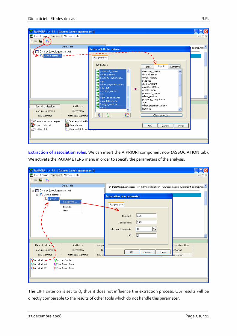
Specifying the status of the variables. In order to specify the status of each descriptor in the
analysis, we use the DEFINE STATUS component. We set all the variables as INPUT.
Didacticiel ‐ Études de cas R.R.
23 décembre 2008 Page 3 sur 21
Extraction of association rules. We can insert the A PRIORI component now (ASSOCIATION tab).
We activate the PARAMETERS menu in order to specify the parameters of the analysis.
The LIFT criterion is set to 0, thus it does not influence the extraction process. Our results will be
directly comparable to the results of other tools which do not handle this parameter.

Didacticiel ‐ Études de cas R.R.
23 décembre 2008 Page 4 sur 21
We click on VIEW menu.
Various indications are available: there are 71 items (attribute‐value pair) into the dataset; 31 of
them have a support >= 0.25 ; we see the number of itemsets of same length i.e. 162 itemsets with
length = 2, etc.; thus, 2986 rules are extracted.
The rules are enumerated in the low part of the report. They are ranked according a decreasing
value of the LIFT criterion.
Didacticiel ‐ Études de cas R.R.
23 décembre 2008 Page 5 sur 21
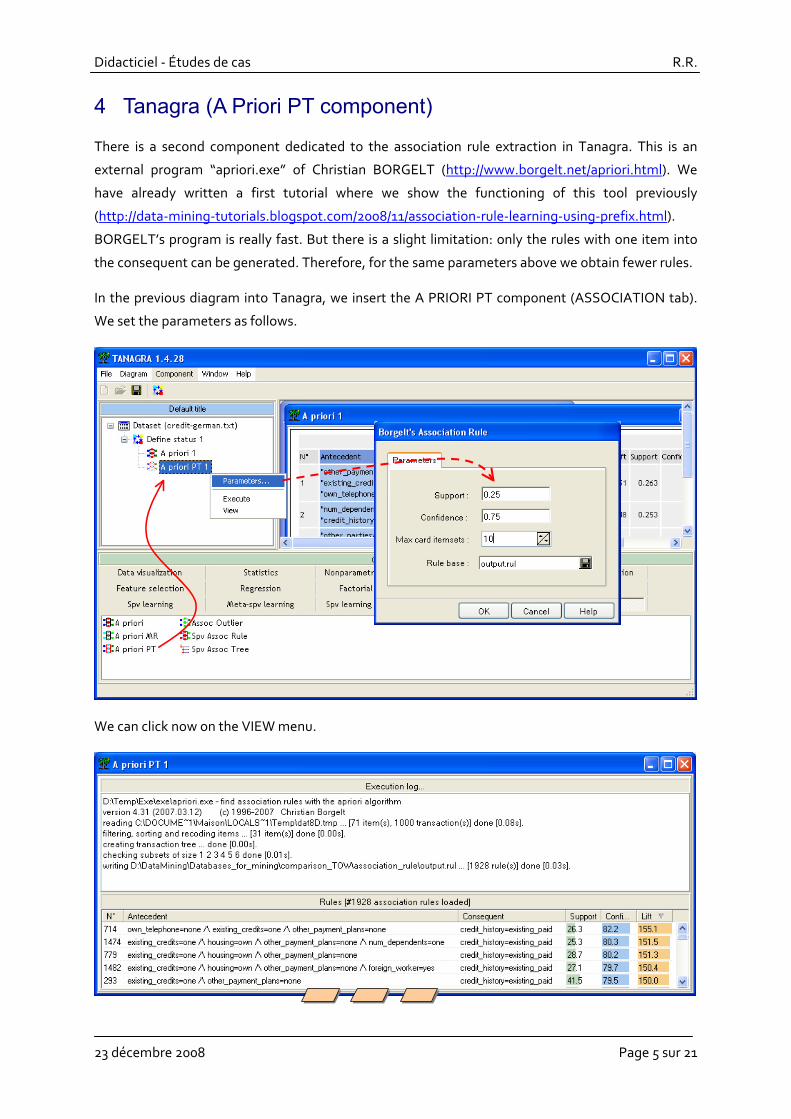
4 Tanagra (A Priori PT component)
There is a second component dedicated to the association rule extraction in Tanagra. This is an
external program “apriori.exe” of Christian BORGELT (http://www.borgelt.net/apriori.html). We
have already written a first tutorial where we show the functioning of this tool previously
(http://data‐mining‐tutorials.blogspot.com/2008/11/association‐rule‐learning‐using‐prefix.html).
BORGELT’s program is really fast. But there is a slight limitation: only the rules with one item into
the consequent can be generated. Therefore, for the same parameters above we obtain fewer rules.
In the previous diagram into Tanagra, we insert the A PRIORI PT component (ASSOCIATION tab).
We set the parameters as follows.
We can click now on the VIEW menu.

Didacticiel ‐ Études de cas R.R.
23 décembre 2008 Page 6 sur 21
In the upper part of the report, we can see the output of the BORGELT’s program (version 4.31). In
the lower part, the rules are enumerated. We can rank the rules according various numeric indicators
by clicking on the column header. Because the component generates the rules with one item into
the consequent, we obtain “only” 1928 rules.
5 R (arules package)
The « arules » package (http://cran.univ‐lyon1.fr/web/packages/arules/index.html) allows extracting
association rules with R (http://www.r‐project.org/). This is also a version of the BORGELT’s
program, with the same limitation. In comparison with Tanagra, we must explicitly prepare the
dataset before. The attribute‐value representation must be transformed into a transactional data
format. The operation is easy… if we read carefully the documentation.
Loading the « arules » package. We use the library(.) command in order to load the package
Data file importation and transformation. We import the dataset with the read.table(.) command,
summary(.) gives some indications about the data characteristics.
We cannot extract rules from a data.frame, we must transform the internal format in "transactions".
We have always 71 items. R gives indications about the density of the dataset. We obtain a large
number of rules if the density of the database is high.

Didacticiel ‐ Études de cas R.R.
23 décembre 2008 Page 7 sur 21
Extraction of rules. The following instructions extract the association rules.
We obtain again the BORGELT’s program output.
Some characteristics of the generated rule base are also available.

Didacticiel ‐ Études de cas R.R.
23 décembre 2008 Page 8 sur 21
Visualization of the rules. The inspect(.) command enables to visualize the details of rules. We
show only the first 10 rules here.
We can also rank the rules according to a rule quality indicator. We show here the first 5 rules
according to the LIFT criterion. We obtain the same rules as the A PRIORI PT component of Tanagra.

Didacticiel ‐ Études de cas R.R.
23 décembre 2008 Page 9 sur 21
6 Orange
Creation of a “schema” and data importation. When we launch Orange, a new empty schema is
available. We add the FILE component (DATA tab). We select the data file.
Rule extraction and visualization. We insert the ASSOCIATION RULES component (ASSOCIATE
tab). We set the parameters of our analysis.

Didacticiel ‐ Études de cas R.R.
23 décembre 2008 Page 10 sur 21
Then we add the ASSOCIATION RULES VIEWER component, we connect the components. We can
now set the connection between FILE and ASSOCIATION RULES. The calculation is launched.
To see the rules, we click on the VIEW menu of the ASSOCIATION RULES VIEWER component.
The visualization window is really original. We can graphically select a group of rules according to a
range of the value of two criteria. Various criteria can be used; we can also rank the rules here.
Didacticiel ‐ Études de cas R.R.
23 décembre 2008 Page 11 sur 21
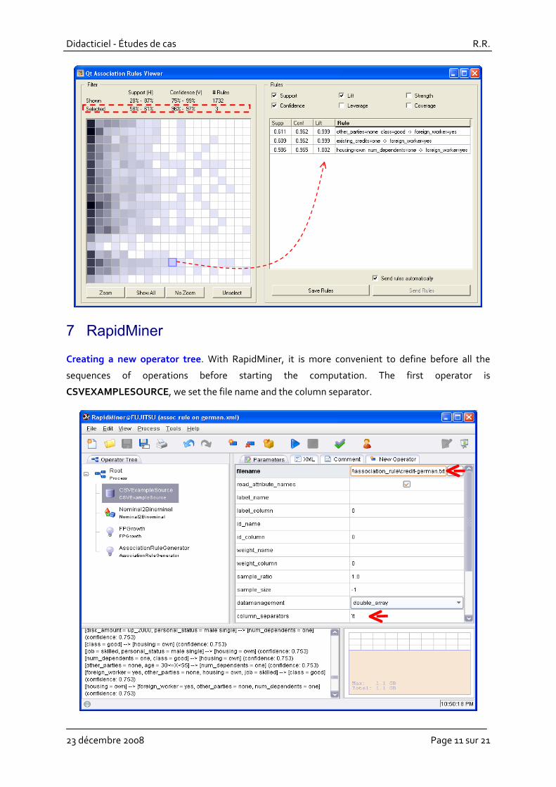
7 RapidMiner
Creating a new operator tree. With RapidMiner, it is more convenient to define before all the
sequences of operations before starting the computation. The first operator is
CSVEXAMPLESOURCE, we set the file name and the column separator.

Didacticiel ‐ Études de cas R.R.
23 décembre 2008 Page 12 sur 21
RapidMiner cannot create association rules from an attribute‐value dataset. We must recode the
variable into a set of binary columns with the NOMINAL2BINOMIAL component.
The extraction is carried out in 2 steps. First, with the FPGROWTH component, we generate the
frequent itemsets. The settings must be defined carefully.
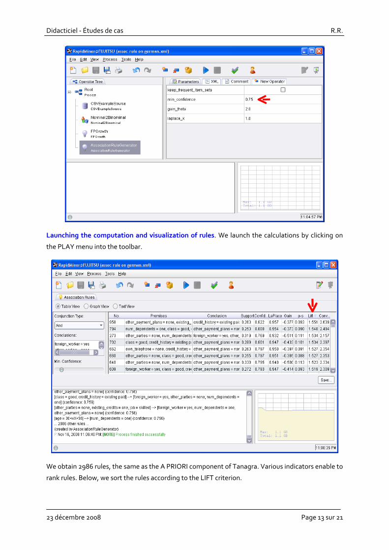
Then, with the ASSOCIATIONRULEGENERATOR, we generate the rules from the itemsets.
Didacticiel ‐ Études de cas R.R.
23 décembre 2008 Page 13 sur 21
Launching the computation and visualization of rules. We launch the calculations by clicking on
the PLAY menu into the toolbar.
We obtain 2986 rules, the same as the A PRIORI component of Tanagra. Various indicators enable to
rank rules. Below, we sort the rules according to the LIFT criterion.

Didacticiel ‐ Études de cas R.R.
23 décembre 2008 Page 14 sur 21
Another option is available. We can filter out the rules according to the presence or absence of an
item or a set of items. This is very useful.
8 Knime
A double data preparation is necessary for KNIME before launching the learning algorithm: a coding
0/1 of the attribute‐value dataset, followed by a transformation into transactional data.
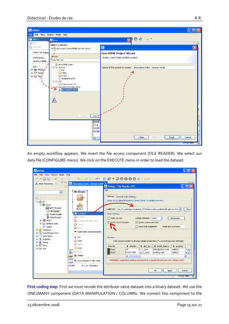
Workflow creation and data importation. We create a new project by clicking on the FILE / NEW
menu. We choose a KNIME project and we specify the name of the project.
Didacticiel ‐ Études de cas R.R.
23 décembre 2008 Page 15 sur 21
An empty workflow appears. We insert the file access component (FILE READER). We select our
data file (CONFIGURE menu). We click on the EXECUTE menu in order to load the dataset.
First coding step. First we must recode the attribute‐value dataset into a binary dataset. We use the
ONE2MANY component (DATA MANIPULATION / COLUMN). We connect this component to the

Didacticiel ‐ Études de cas R.R.
23 décembre 2008 Page 16 sur 21
previous one. We add an INTERACTIVE TABLE component (DATA VIEWS), that we connect to
ONE2MANY, in order to view the new dataset.
There are 90 columns now. To the previous 19 variables are added 71 binary variables.
Second coding step. The first transformation is not enough. We must go through an internal format
specific using the BITVECTOR component (DATA MANIPULATION / COLUMN). We connect it to
ONE2MANY. We click on the CONFIGURE menu, we select only the binary variables.

Didacticiel ‐ Études de cas R.R.
23 décembre 2008 Page 17 sur 21
By clicking on the EXECUTE AND OPEN VIEW menu, we obtain a description of the generated
transactional dataset.
To obtain the information of density of R, we make 19000/(19000+52000) = 26.76%.
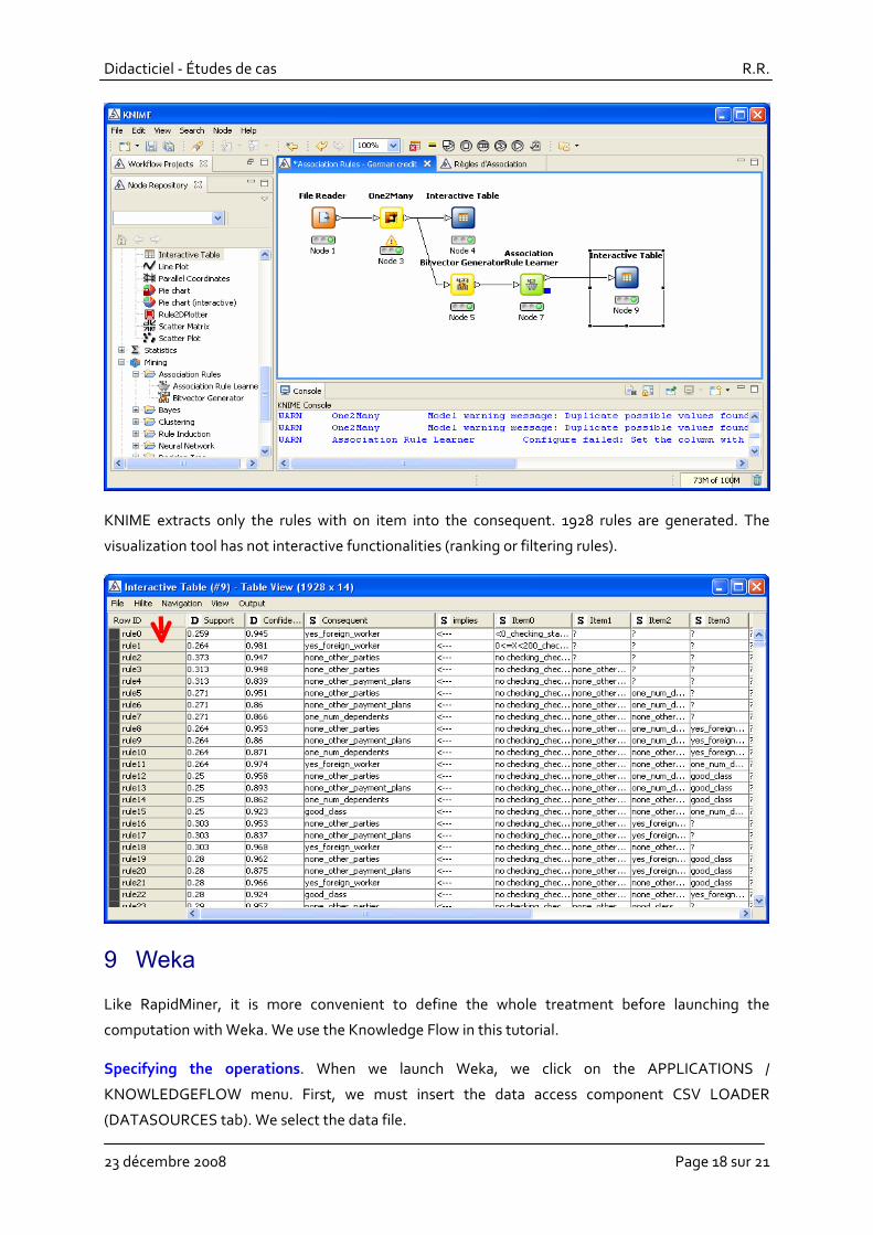
Extraction of rules. We use the ASSOCIATION RULE LEARNER component in order to extract rules.
We set the following parameters.
0.25
0.75
The INTERACTIVE TABLE component enables to visualize the rules.
Didacticiel ‐ Études de cas R.R.
23 décembre 2008 Page 18 sur 21
KNIME extracts only the rules with on item into the consequent. 1928 rules are generated. The
visualization tool has not interactive functionalities (ranking or filtering rules).
9 Weka
Like RapidMiner, it is more convenient to define the whole treatment before launching the
computation with Weka. We use the Knowledge Flow in this tutorial.
Specifying the operations. When we launch Weka, we click on the APPLICATIONS /
KNOWLEDGEFLOW menu. First, we must insert the data access component CSV LOADER
(DATASOURCES tab). We select the data file.

Didacticiel ‐ Études de cas R.R.
23 décembre 2008 Page 19 sur 21
We add the APRIORI component (ASSOCIATIONS tab). We connect the previous component to this
one. We click on the CONFIGURE menu in order to define the parameters.
Setting NUMRULES to 1000 removes the restriction on the number of generated rules. We add then
the TEXT VIEWER component in order to visualize the rules.

Didacticiel ‐ Études de cas R.R.
23 décembre 2008 Page 20 sur 21
We launch the calculations by clicking on the START LOADING menu of… the CSV LOADER
component into the knowledge flow.
To visualize the results, we click on the SHOW RESULTS menu of the TEXTVIEWER component.
Like the A PRIORI component of Tanagra, we obtain 2986 rules.

Didacticiel ‐ Études de cas R.R.
23 décembre 2008 Page 21 sur 21
10 Conclusion
All software presented in this tutorial can extract association rules from a data file in an "individuals
x variables" format. For some of them, a data preparation is required before to produce a
transactional data format. This is not always obvious, especially when the software is not well
documented. I admit to having groping a bit. But finally, once the data are correctly generated, the
software produced similar results. This is what matters.