Tanagra Tutorials R.R.

2 janvier 2018 Page 1

1 Introduction

Processing the sparse data file format with Tanagra1.

The data to be processed with machine learning algorithms are increasing in size. Especially when we need to process unstructured data. The data preparation (e. g. the use of a bag of words representation in text mining) leads to the creation of large data tables where, often, the number of columns (descriptors) is higher than the number of rows (observations). With the singularity that the table contains many zero values. In this context, storing all these zero values into the data file is not opportune. A data compression strategy without loss of information must be implemented, which must remain simple so that the file is readable with a text editor.

In this tutorial, we describe the use of the sparse data file format handled by Tanagra (from the version 1.4.4). It is based on the file format processed by famous libraries for machine learning (svmlight, libsvm, libcvm)2. We show its use in a text categorization process applied to the Reuters database, well known in data mining3. We will observe that the use of this kind of sparse format enables to reduce dramatically the data file size.

2 The “sparse” data file format

2.1 From attribute-value table format to the sparse format

In text mining, the starting point is always a document collection. But the machine learning algorithms cannot process the raw documents. We must transform the document collection in the attribute value table which is the usual data representation. The bag-of words model is definitely the most popular approach.

Let us consider an example to detail the approach. We have a collection of 3 documents (in French):

A. “Le soleil brille dans le ciel” B. “Le ciel est bleu” C. “Voilà le produit pour faire briller”

1 The French version of this tutorial is written in May 2012. Unfortunately, it seems that some websites links are

broken. I did not find the updated links.

2 http://svmlight.joachims.org/ ; http://www.csie.ntu.edu.tw/~cjlin/libsvm/ ; http://c2inet.sce.ntu.edu.sg/ivor/cvm.html

3 http://kdd.ics.uci.edu/databases/reuters21578/reuters21578.html

Tanagra Tutorials R.R.

2 janvier 2018 Page 2

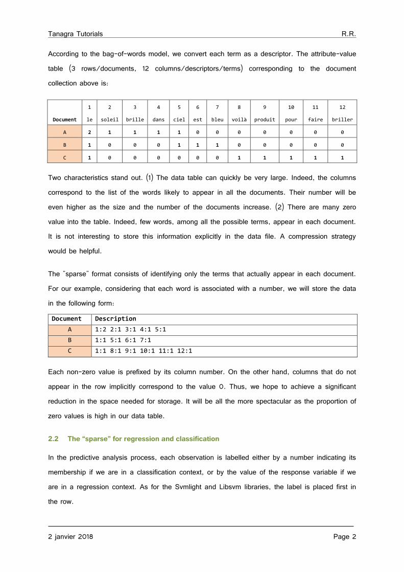
According to the bag-of-words model, we convert each term as a descriptor. The attribute-value table (3 rows/documents, 12 columns/descriptors/terms) corresponding to the document collection above is:

Document

1

le

2

soleil

3

brille

4

dans

5

ciel

6

est

7

bleu

8

voilà

9

produit

10

pour

11

faire

12

briller

A 2 1 1 1 1 0 0 0 0 0 0 0

B 1 0 0 0 1 1 1 0 0 0 0 0

C 1 0 0 0 0 0 0 1 1 1 1 1

Two characteristics stand out. (1) The data table can quickly be very large. Indeed, the columns correspond to the list of the words likely to appear in all the documents. Their number will be even higher as the size and the number of the documents increase. (2) There are many zero value into the table. Indeed, few words, among all the possible terms, appear in each document. It is not interesting to store this information explicitly in the data file. A compression strategy would be helpful.

The "sparse" format consists of identifying only the terms that actually appear in each document. For our example, considering that each word is associated with a number, we will store the data in the following form: Document Description

A 1:2 2:1 3:1 4:1 5:1

B 1:1 5:1 6:1 7:1

C 1:1 8:1 9:1 10:1 11:1 12:1

Each non-zero value is prefixed by its column number. On the other hand, columns that do not appear in the row implicitly correspond to the value 0. Thus, we hope to achieve a significant reduction in the space needed for storage. It will be all the more spectacular as the proportion of zero values is high in our data table.

2.2 The “sparse” for regression and classification

In the predictive analysis process, each observation is labelled either by a number indicating its membership if we are in a classification context, or by the value of the response variable if we are in a regression context. As for the Svmlight and Libsvm libraries, the label is placed first in the row.

Tanagra Tutorials R.R.

2 janvier 2018 Page 3

For the document collection above, let us consider that the documents A and B belong to the first class “1”, and C belongs to “-1”. Our data file has the following appearance: 1 1:2 2:1 3:1 4:1 5:1 1 1:1 5:1 6:1 7:1 -1 1:1 8:1 9:1 10:1 11:1 12:1

Note: Whether in classification or regression, the label always corresponds to a numerical value in the file. A recoding will be necessary into Tanagra to consider that it is an indicator of the class membership.

2.3 The “reuters (money fx)” database

We process the Reuters database. It is a classic of text categorization problem. We have a collection of news. Each of them is indexed by one or more categories (TOPICS). The following document for example is associated to the topics "money-fx" and "interest".

<REUTERS TOPICS="YES" LEWISSPLIT="TRAIN" CGISPLIT="TRAINING-SET" OLDID="5764" NEWID="221"> <DATE>26-FEB-1987 21:05:51.60</DATE> <TOPICS><D>money-fx</D><D>interest</D></TOPICS> <PLACES><D>japan</D></PLACES> <PEOPLE></PEOPLE> <ORGS></ORGS> <EXCHANGES></EXCHANGES> <COMPANIES></COMPANIES> <UNKNOWN> &#5;&#5;&#5;RM &#22;&#22;&#1;f0438&#31;reute u f BC-AVERAGE-YEN-CD-RATES 02-26 0096</UNKNOWN> <TEXT>&#2; <TITLE>AVERAGE YEN CD RATES FALL IN LATEST WEEK</TITLE> <DATELINE> TOKYO, Feb 27 - </DATELINE><BODY>Average interest rates on yen certificates of deposit, CD, fell to 4.27 pct in the week ended February 25 from 4.32 pct the previous week, the Bank of Japan said. New rates (previous in brackets), were - Average CD rates all banks 4.27 pct (4.32) Money Market Certificate, MMC, ceiling rates for the week starting from March 2 3.52 pct (3.57) Average CD rates of city, trust and long-term banks Less than 60 days 4.33 pct (4.32) 60-90 days 4.13 pct (4.37) Average CD rates of city, trust and long-term banks 90-120 days 4.35 pct (4.30) 120-150 days 4.38 pct (4.29) 150-180 days unquoted (unquoted) 180-270 days 3.67 pct (unquoted) Over 270 days 4.01 pct (unquoted) Average yen bankers' acceptance rates of city, trust and long-term banks 30 to less than 60 days unquoted (4.13) 60-90 days unquoted (unquoted) 90-120 days unquoted (unquoted) REUTER &#3;</BODY></TEXT> </REUTERS>

The objective of modeling is to learn from labelled data a classification function that automatically associates a new unseen instance to a class. In practice, we prefer to consider the treatment

Tanagra Tutorials R.R.

2 janvier 2018 Page 4

from a binary perspective in order to simplify the process i.e. we want to know if a text belongs to a specific category. Into the learning set, "positive" documents are those related to the target category; "negative" documents are the others.

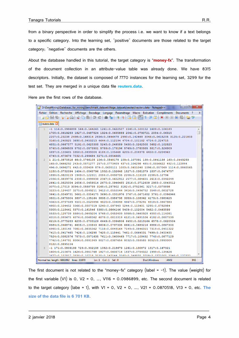
About the database handled in this tutorial, the target category is “money-fx”. The transformation of the document collection in an attribute-value table was already done. We have 8315 descriptors. Initially, the dataset is composed of 7770 instances for the learning set, 3299 for the test set. They are merged in a unique data file reuters.data.

Here are the first rows of the database.

The first document is not related to the “money-fx” category (label = -1). The value (weight) for the first variable (V1) is 0, V2 = 0, …, V116 = 0.0986899, etc. The second document is related to the target category (labe = 1), with V1 = 0, V2 = 0, …, V21 = 0.0870518, V13 = 0, etc. The size of the data file is 6 701 KB.

Tanagra Tutorials R.R.

2 janvier 2018 Page 5

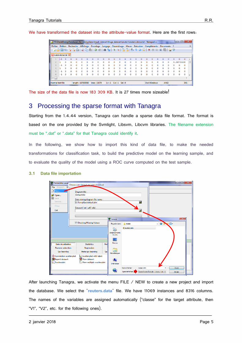
We have transformed the dataset into the attribute-value format. Here are the first rows:

The size of the data file is now 183 309 KB. It is 27 times more sizeable!

3 Processing the sparse format with Tanagra

Starting from the 1.4.44 version, Tanagra can handle a sparse data file format. The format is based on the one provided by the Svmlight, Libsvm, Libcvm libraries. The filename extension must be “.dat” or “.data” for that Tanagra could identify it.

In the following, we show how to import this kind of data file, to make the needed transformations for classification task, to build the predictive model on the learning sample, and to evaluate the quality of the model using a ROC curve computed on the test sample.

3.1 Data file importation

After launching Tanagra, we activate the menu FILE / NEW to create a new project and import the database. We select the "reuters.data" file. We have 11069 instances and 8316 columns. The names of the variables are assigned automatically (“classe” for the target attribute, then “V1”, “V2”, etc. for the following ones).

Tanagra Tutorials R.R.

2 janvier 2018 Page 6

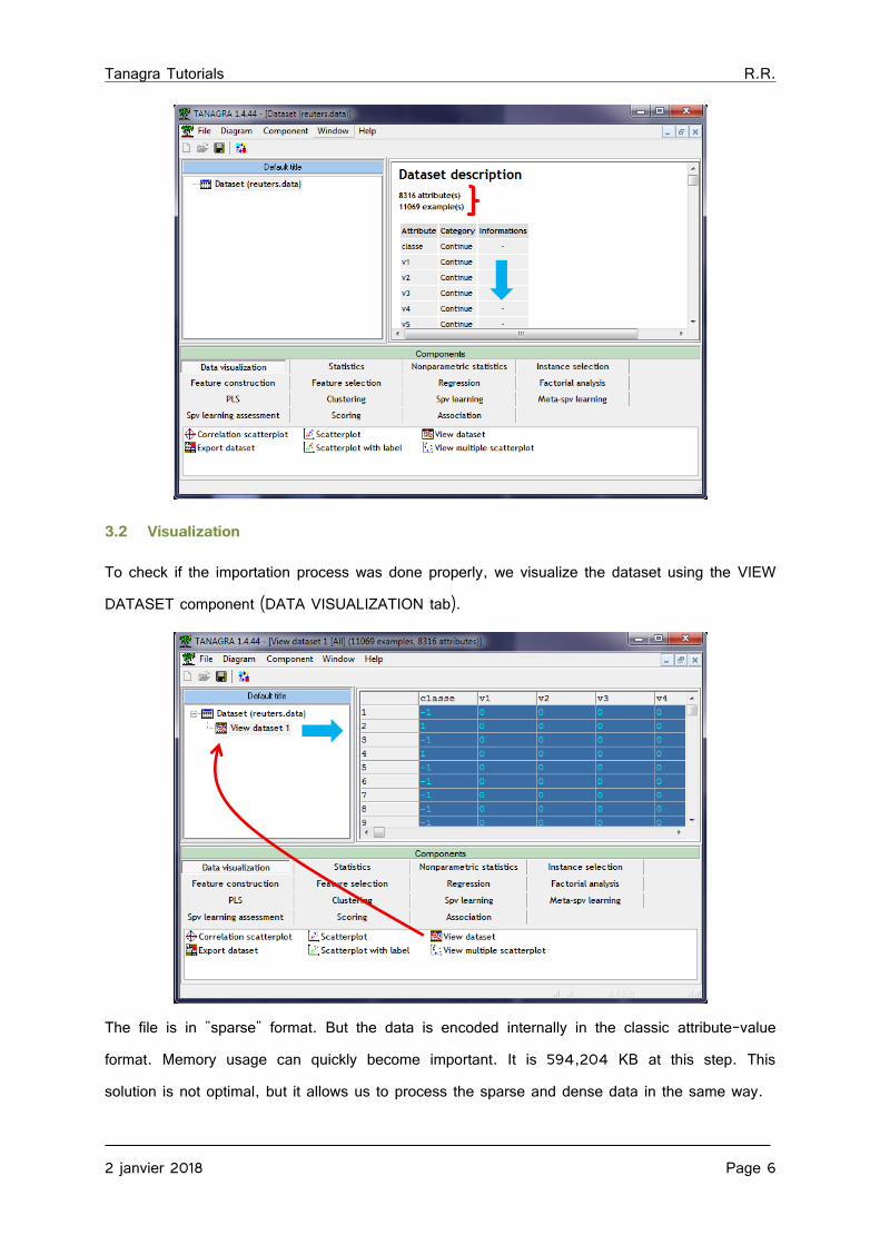
3.2 Visualization

To check if the importation process was done properly, we visualize the dataset using the VIEW DATASET component (DATA VISUALIZATION tab).

The file is in "sparse" format. But the data is encoded internally in the classic attribute-value format. Memory usage can quickly become important. It is 594,204 KB at this step. This solution is not optimal, but it allows us to process the sparse and dense data in the same way.

Tanagra Tutorials R.R.

2 janvier 2018 Page 7

3.3 Recoding the target attribute

Because the "classe" variable is numeric, we cannot use it directly for the classification process. We must recode it. For that, we insert the DEFINE STATUS component into the diagram and we set the “classe” variable as INPUT.

Then we add the CONT TO DISC (FEATURE CONSTRUCTION tab) component. It recodes the variable by assigning a category for each distinct value.

Tanagra Tutorials R.R.

2 janvier 2018 Page 8

After we click on the contextual menu VIEW, we observe that the new variable C2D_CLASSE_1 is categorical with 2 values {“-1”, “1”}.

3.4 Classes distribution

We can compute the classes distribution. We insert the DEFINE STATUS into the diagram. We set the new attribute C2D_CLASSE_1 as INPUT.

Then, we add the UNIVARIATE DISCRETE STAT (STATISTICS tab) component.

We observe that the classes are rather imbalanced (6.48% of instances for the target value “1”).

Tanagra Tutorials R.R.

2 janvier 2018 Page 9

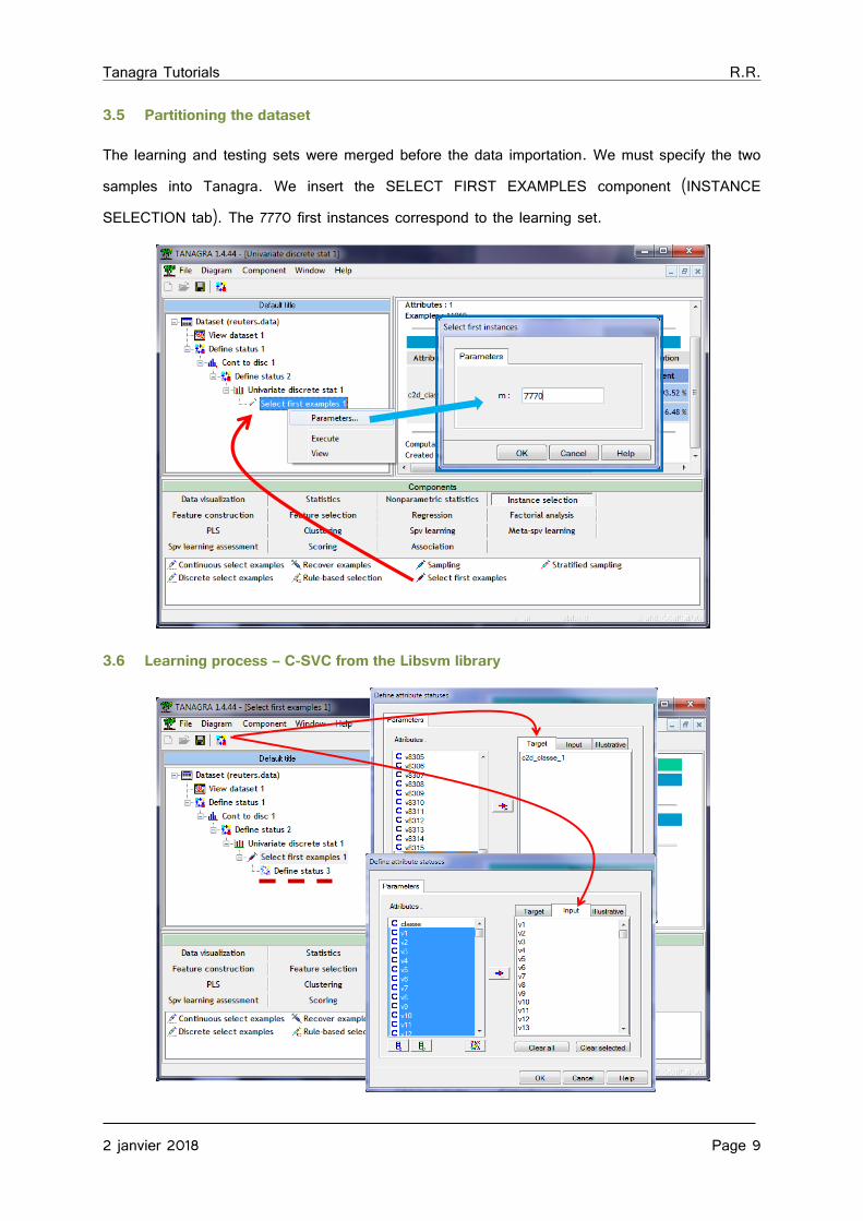
3.5 Partitioning the dataset

The learning and testing sets were merged before the data importation. We must specify the two samples into Tanagra. We insert the SELECT FIRST EXAMPLES component (INSTANCE SELECTION tab). The 7770 first instances correspond to the learning set.

3.6 Learning process – C-SVC from the Libsvm library

Tanagra Tutorials R.R.

2 janvier 2018 Page 10

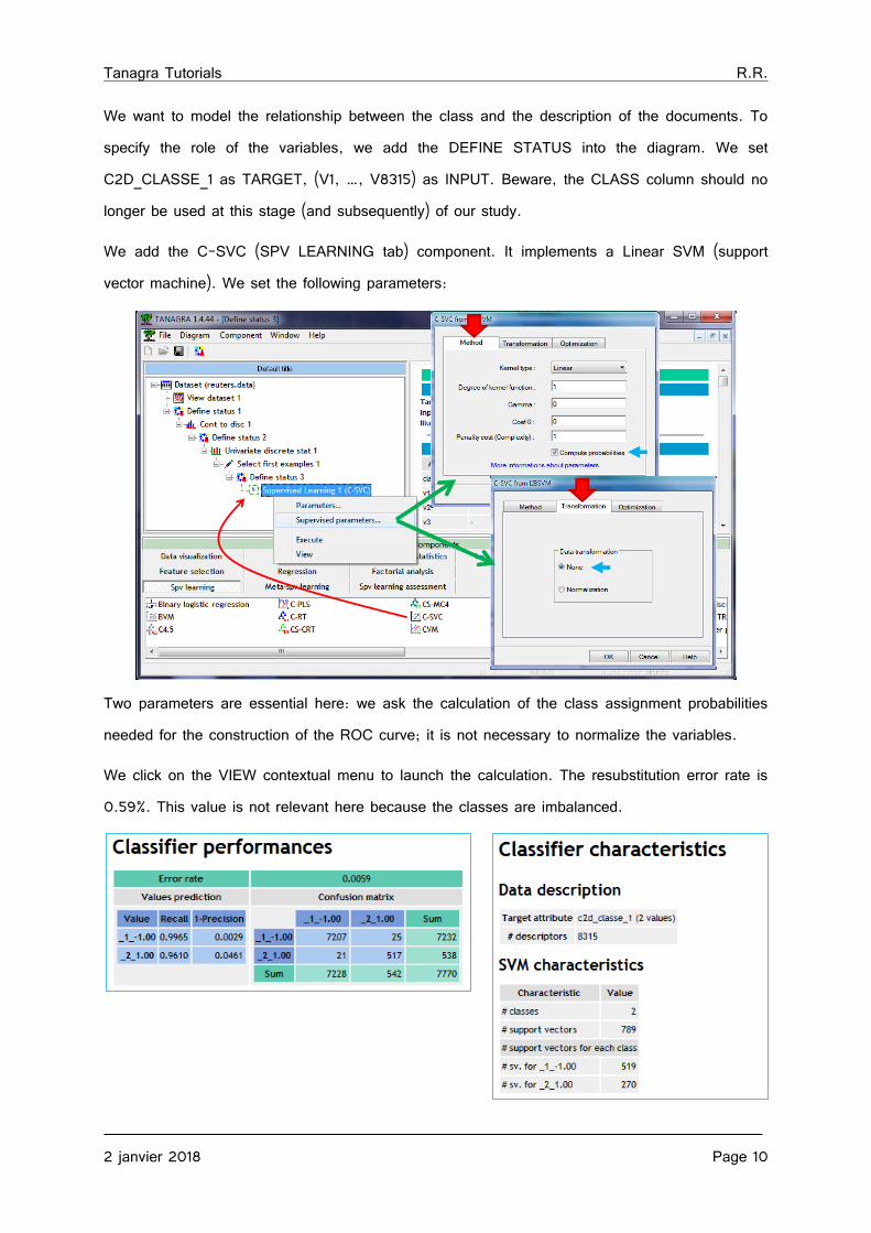
We want to model the relationship between the class and the description of the documents. To specify the role of the variables, we add the DEFINE STATUS into the diagram. We set C2D_CLASSE_1 as TARGET, (V1, …, V8315) as INPUT. Beware, the CLASS column should no longer be used at this stage (and subsequently) of our study.

We add the C-SVC (SPV LEARNING tab) component. It implements a Linear SVM (support vector machine). We set the following parameters:

Two parameters are essential here: we ask the calculation of the class assignment probabilities needed for the construction of the ROC curve; it is not necessary to normalize the variables.

We click on the VIEW contextual menu to launch the calculation. The resubstitution error rate is 0.59%. This value is not relevant here because the classes are imbalanced.

Tanagra Tutorials R.R.

2 janvier 2018 Page 11

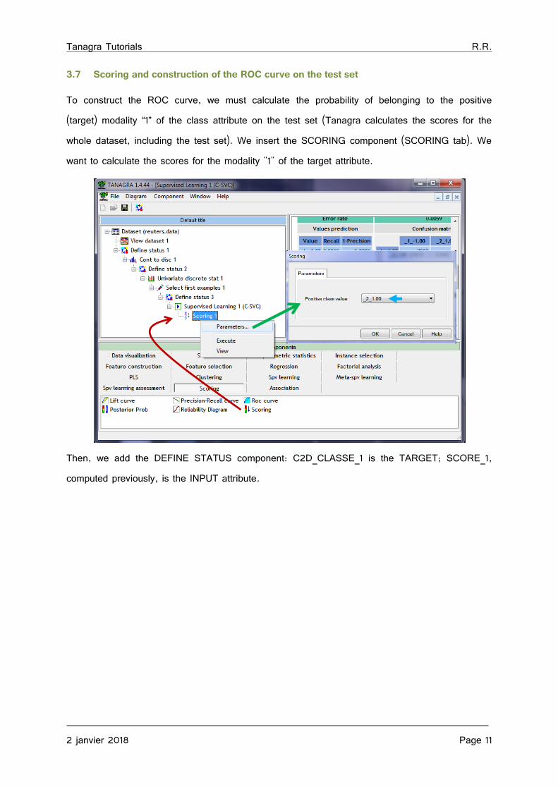
3.7 Scoring and construction of the ROC curve on the test set

To construct the ROC curve, we must calculate the probability of belonging to the positive (target) modality “1” of the class attribute on the test set (Tanagra calculates the scores for the whole dataset, including the test set). We insert the SCORING component (SCORING tab). We want to calculate the scores for the modality "1" of the target attribute.

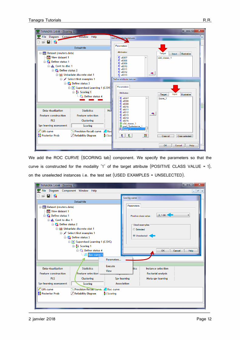
Then, we add the DEFINE STATUS component: C2D_CLASSE_1 is the TARGET; SCORE_1, computed previously, is the INPUT attribute.

Tanagra Tutorials R.R.

2 janvier 2018 Page 12

We add the ROC CURVE (SCORING tab) component. We specify the parameters so that the curve is constructed for the modality "1" of the target attribute (POSITIVE CLASS VALUE = 1), on the unselected instances i.e. the test set (USED EXAMPLES = UNSELECTED).

Tanagra Tutorials R.R.

2 janvier 2018 Page 13

We see that our model is efficient. The area under curve (AUC) is equal to 0.983 i.e. a randomly chosen positive instance (of the class "1") has 98.3% chances of having a higher score than a negative instance (of the class "-1").

3.8 Comparison with logistic regression

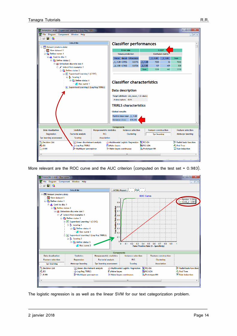
We want to lead the same analysis but using logistic regression. We use an implementation of TRIRLS approach (iterative reweighted least squares algorithm for logistic regression4). We added the AUTONLAB library as a DLL in the Tanagra (from the 1.4.44 version) (http://autonlab.org/autonweb/10538). If the library seems not really efficient on standard dataset (few variables, large number of instances), it seems much better on wide dataset (large number of descriptors).

We insert the LOG-REG TRIRLS (SPV LEARNING tab) component into the diagram. We obtain the model deviance (-2LL = 878.242) and the coefficients of the regression equation. The resubstitution error rate is 2.07%. But we know that this criterion is not relevant in our context.

4 https://en.wikipedia.org/wiki/Iteratively_reweighted_least_squares

Tanagra Tutorials R.R.

2 janvier 2018 Page 14

More relevant are the ROC curve and the AUC criterion (computed on the test set = 0.983).

The logistic regression is as well as the linear SVM for our text categorization problem.

Tanagra Tutorials R.R.

2 janvier 2018 Page 15

4 Sparse data file processing with other tools

Of course, other data mining tools can handle the sparse data file format (Svmlight, Libsvm). We describe briefly in this section the functionalities of RapidMiner and Weka.

4.1 RapidMiner

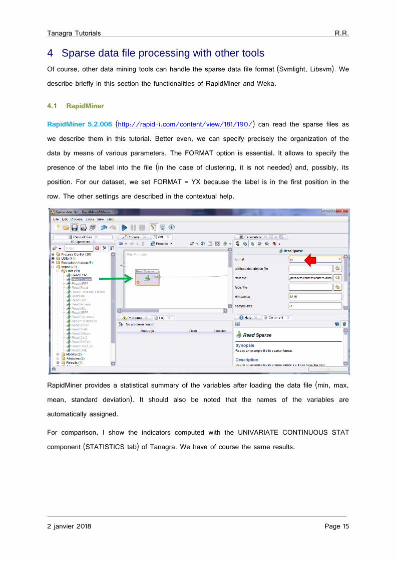
RapidMiner 5.2.006 (http://rapid-i.com/content/view/181/190/) can read the sparse files as we describe them in this tutorial. Better even, we can specify precisely the organization of the data by means of various parameters. The FORMAT option is essential. It allows to specify the presence of the label into the file (in the case of clustering, it is not needed) and, possibly, its position. For our dataset, we set FORMAT = YX because the label is in the first position in the row. The other settings are described in the contextual help.

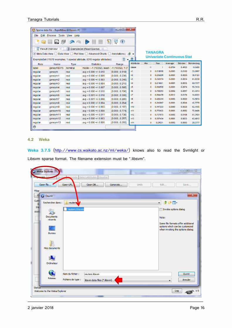
RapidMiner provides a statistical summary of the variables after loading the data file (min, max, mean, standard deviation). It should also be noted that the names of the variables are automatically assigned.

For comparison, I show the indicators computed with the UNIVARIATE CONTINUOUS STAT component (STATISTICS tab) of Tanagra. We have of course the same results.

Tanagra Tutorials R.R.

2 janvier 2018 Page 16

4.2 Weka

Weka 3.7.5 (http://www.cs.waikato.ac.nz/ml/weka/) knows also to read the Svmlight or Libsvm sparse format. The filename extension must be “.libsvm”.

TANAGRA

Univariate Continuous Stat

Tanagra Tutorials R.R.

2 janvier 2018 Page 17

5 Conclusion

The "sparse" data file format enables to reduce the file size by adopting a customized data representation. Like any compression algorithm, there are contexts where it generates zero or even negative gains. When we are faced with a standard database (called also “dense database”), with a very small proportion of zero values, it is not efficient. On the other hand, it becomes relevant when we handle pre-processed data from a collection of unstructured data, where the descriptors are generated automatically with a large proportion of zero values. We have taken the example of text mining context in this tutorial.