Embed Size (px)
Citation preview

Ensemble Methods in Large Vocabulary Continuous
Speech Recognition
_________________________________
A thesis presented to the Faculty of the Graduate School
University of Missouri-Columbia
_________________________________
In Partial Fulfillment
Of the Requirements for the Degree
Master of Science
_________________________________
by
Xin Chen
Dr. Yunxin Zhao, Advisor
May 2008

The undersigned, appointed by the dean of the Graduate School, have examined the
thesis entitled
Ensemble Methods in Large Vocabulary Continuous Speech Recognition
Presented by Xin Chen,
a candidate for the degree of master of computer science,
and hereby certify that, in their opinion, it is worthy of acceptance.
Professor Yunxin Zhao
Professor Wenjun Zeng
Professor Dominic Ho

Acknowledgements
First of all, I would like to thank my advisor, Dr. Yunxin Zhao. It is a great honor
to be her student. Her inspirations and help light me up in the ASR field. I feel so lucky
for what I have.
And many thanks to Dr. Dominic Ho and Dr. Wenjun Zeng for their support and
service as my committee members. I really appreciate their help for reviewing my thesis
and giving me valuable advices.
Also I want to thank my grandmother and my parents. Their supports from the other
side of the earth give me courage and passion.
Much respects are paid to my current officemates Yi Zhang, Xie Sun, as well as
previous officemates, Rong Hu, Jian Xue, Lily Che. I got lots of help from them and it
has been a pleasure working with them.
ii

TABLE OF CONTENTS
Acknowledgements ............................................................................................... ii
List of Figures ......................................................................................................... v
List of Tables ......................................................................................................... vi
Abstract ................................................................................................................... viii
Chapter 1 ................................................................................................................... 1
Statistical Speech Recognition .................................................................................. 1
1.1 General statistical speech recognition ....................................................... 1
1.2 Pre-processing of Speech .......................................................................... 3
1.3 Language Modeling ................................................................................... 4
1.4 Acoustic Modeling .................................................................................... 6
1.4.1 Hidden Markov Model (HMM) in speech recognition ............................ 7
1.5 Pronunciation dictionary and lexical tree ................................................ 10
1.6 Viterbi Algorithm .................................................................................... 12
1.7 Summery ................................................................................................. 13
Chapter 2 ................................................................................................................. 15
Explicit Phonetic Decision Tree Tying ................................................................... 15
2.1 Phonetic Decision Tree background ....................................................... 18
2.2 Explicit PDT tying .................................................................................. 21
2.3 Ensemble Classifier based on Explicit PDT tying .................................. 25
2.4 Hierarchical Ensemble Classifier based on different mixture size ......... 26
iii

Chapter 3 ................................................................................................................. 28
Data Sampling in Ensemble Acoustic Modeling .................................................... 28
3.1 Ensemble classifier for acoustic score combination ............................... 28
3.2 Sampling training data to generate an ensemble of acoustic model ....... 31
3.3 Cross-Validation Sampling ..................................................................... 32
3.4 Random Sampling ................................................................................... 34
3.5 Combiner design ..................................................................................... 34
Chapter 4 ................................................................................................................. 37
Experiments and Analysis ....................................................................................... 37
4.1 Experiment Setup on Telemedicine Automatic Captioning System ....... 37
4.2 Experimental results for phoneme sharing explicit PDT tying ............... 39
4.3 Experimental results for multiple acoustic models based on EPDT ....... 43
4.4 Experimental results for Cross Validation sampling ............................... 44
4.5 Experimental results for Random Sampling ........................................... 49
4.6 Experimental results for combining methods .......................................... 51
4.7 Experimental results for different mixture size based ensemble method 52
Chapter 5 ................................................................................................................. 54
Conclusion .............................................................................................................. 54
Reference ................................................................................................................ 56
iv
List of Figures
Figure 1.1 An example of HMM for a phoneme model using Gaussian pdf in each
emitting state. ...................................................................................................... 8
Figure 1.2 Part of a sample dictionary ...................................................................... 11
Figure 1.3 Fraction of a lexical tree .......................................................................... 12
Figure 1.4 Diagram of an automatic speech recognition system. ............................. 14
Figure 2.1 The three levels of speech recognition .................................................... 16
Figure 2.2 An example of decision tree construction ............................................... 20
Figure 2.3 Explicit decision tree triphone tying ........................................................ 23
Figure 2.4 Triphone tying example ........................................................................... 25
Figure 3.1 ROVOR framework................................................................................. 29
Figure 3.2 Ensemble framework in telehealth system .............................................. 30
Figure 3.3 Sampling data in generating ensemble classifiers ................................... 31
Figure 3.4 5-fold Cross Validation ........................................................................... 33
Figure 4.1 The block diagram of Automatic Captioning System for Telemedicine . 37
Figure 4.2 The effect of different mixture sizes on word accuracy .......................... 48
v

List of Tables
Table 2.1 One example of a state clustering in EPDT in our telehealth task ........... 24
Table 4.1 Datasets used: speech (min.)/text (no. of words). ..................................... 38
Table 4.2 Word accuracy obtained from EPDT tying 1 ........................................... 39
Table 4.3 Word accuracy obtained from EPDT tying 2 ........................................... 40
Table 4.4 Word accuracy obtained from the extreme case of EPDT tying .............. 42
Table 4.5 Word accuracy obtained from combining the Baseline and the 6-Tree
models ............................................................................................................... 43
Table 4.6 Word accuracy obtained from combining the Baseline model and the .... 44
3-Tree model and the 6-Tree model .......................................................................... 44
Table 4.7 Word accuracy obtained from the Cross Validation based ensemble
acoustic model, Fold size = 10 .......................................................................... 45
Table 4.8 The effectiveness of 10-fold CV base classifiers on recognition
performance ...................................................................................................... 46
Table 4.9 The effectiveness of different fold sizes on recognition performance ...... 47
Table 4.10 The effectiveness of Different mixture sizes on word accuracy
performance ...................................................................................................... 48
Table 4.11 Word accuracy obtained from the ensemble models that are generated
through Random Sampling without replacement ............................................. 50
Table 4.12: m-best performance ............................................................................... 51
Table 4.13: m-Trimmed average performance ......................................................... 51
Table 4.14: Maximum Likelihood Estimation performance ..................................... 52
vi

Table 4.15 Hierarchical ensemble acoustic model based on 10 models from mixture
size 6 to mixture size 24 on word accuracy test................................................ 53
vii

Abstract
Combining a group of classifiers and therefore improving the overall classification
performance is a young and promising direction in Large Vocabulary Continuous Speech
Recognition (LVCSR). Previous works on acoustic modeling of speech signals such as
Random Forests (RFs) of Phonetic Decision Trees (PDTs) has produced significant
improvements in word recognition accuracy. In this thesis, several new ensemble
approaches are proposed for LVCSR and experimental evaluations have shown absolute
accuracy gains up to 2.3% over the conventional PDT-based acoustic models in our
telehealth conversational speech recognition task.
Unlike the implicit PDT based states tying that has been used in most ASR systems
as well as in the recent RFs based PDTs, this author considers that explicit PDT (EPDT)
tying that allows Phoneme data Sharing (PS) may be superior in capturing pronunciation
variations. The author adopted the idea of combining multiple acoustic models and
applied this idea to the EPDT models. A combination of EPDT and the implicit PDT
models has been investigated to reduce phone confusions that may be introduced by the
EPDT model. A 1.3% absolute gain on word accuracy is observed in this experiment on
the telehealth task.
Data sampling is one of the primary ways to generate different classifiers for an
ensemble classifier. In this thesis, Cross Validation (CV) based data sampling is proposed,
and random sampling without replacement is used as a reference for comparison. With
different datasets generated by data sampling, different PDTs and therefore different
viii

ix
Gaussian mixture models are generated, and the diversity of the multiple models helps
improve recognition accuracy. When a 10-fold-CV is used, a 2.3% absolute gain in word
recognition accuracy is obtained. Several experimental parameter settings and combining
methods have been investigated in the experiments and the findings are discussed in this
thesis.
The word accuracy performance improvement achieved in this thesis work is
significant and the techniques have been integrated in the telemedicine automatic
captioning system developed by the SLIPL group of the University of Missouri –
Columbia.

Chapter 1
Statistical Speech Recognition
1.1 General statistical speech recognition
Speech is the most convenient everyday communication method among humans,
and it is a very promising interface between computer and human. After a half century of
evolution [1], Automatic Speech Recognition (ASR) systems nowadays are finding
applications in everyday’s life. For example, automatic customer service system allows
people to use voice to select a restaurant menu. Another example is our telemedicine
automatic captioning project: ASR is helping people who have hearing loss to directly
read a captioned message that a doctor’s speech conveys over a long distance. ASR is a
very meaningful field and we are devoting our passion on enhancing the recognition
accuracy, the decoding speed as well as the system functionality.
Generally, we can simply describe speech recognition as a time series classification
problem. It attempts to find an optimized word sequence that best match a speech
utterance. The most successful method of speech recognition is based on Bayesian
decision theory [2],
1
( ) ( ) ( | )( | )( ) ( ) ( | )
k
i
P x Cj P Cj P x CjP Cj xP x P Ci P x Ci
=
∩= =
∑, (1.1)
where given a data sample x, we calculate the posterior probability of the class Cj, from
the prior probabilities of , and the conditional probabilities of x given Ci, i =
1, 2,…, k. When we apply Bayes rule to our speech recognition problem, we can rewrite
the decision problem as:
kCCC ,,, 21
1

( | ) ( )ˆ arg max ( | ) arg max arg max ( | ) ( )( )W W W
p O W p W eW p W O p O W p Wp O
α β
eα β= = =
(1.2)
where is the sequence of words (with unknown length n) in an
utterance produced by the speaker which generates the acoustic feature vector
sequence ; p(W), usually called the language model, is the a priori
probability of the word sequence W, which is independent of the observation O; p(O) is
the a priori probability of the observed speech utterance O, which is independent of all
word sequence hypotheses, and so it can be ignored in the last line of formula (1.2);
p(O|W) is the probability that the speaker produces the acoustic feature vector sequence
O if W is the intended word sequence.
nwwwW ,,, 21=
ToooO ,,, 21=
Statistical modeling for estimating p(W) is called language modeling. It concerns
the prior probability of a word sequence W in a sentence. The most commonly used
language model is N-gram, which will be discussed in Section 1.3.
Statistical modeling for estimating p(O|W) is called acoustic modeling. Here W is
usually decomposed into sub words such as phonemes or syllables since they are more
trainable from a finite amount of speech data. We use lexical trees to represent words by
sub-words, usually phonemes. The most commonly used acoustic model is Hidden
Markov Model (HMM) of Context-Dependent (CD) phones. We discuss the details of
acoustic modeling in Section 1.4.
In addition, the α in ( )p W α is referred to as a language model scale factor, which
is used to balance the scores of acoustic model and language model. The parameter eβ is
called word insertion penalty, which is used to control the length of the word hypothesis
2
sequence. These parameters are extremely important in controlling the performance of an
ASR system and therefore should be tuned before the speech recognition system is
deployed in real applications.
Speech recognition engine works by using Viterbi algorithm [3] to search over a
large hypothesis space, determining the best word sequence that has the highest
probability of generating the speech utterance. This part will be discussed in section 1.6.
1.2 Pre-processing of Speech
Speech signals, which are waveforms sampled at a certain clock rate, are not
suitable to be directly used in training acoustic models. Pre-processing is such a
procedure that converts the original waveform of speech into the type of presentation that
only contains necessary information for speech recognition. Typically, the speech sound
waves are captured by a microphone and converted to electrical signals. Then Analog-to-
digital conversion samples speech signal at discrete time intervals (e.g. sampling
rate=16k), which becomes the input to an ASR system. The sampled data is used to
generate feature vectors. This process is called feature analysis. Generally, a feature
vector is computed per 10ms time, from an overlapped sliding window of 20 to 25 ms.
Commonly used features are as follows:
1 Linear Predictive Coefficient (LPC) – a speech sample at time t is approximated
as a linear combination of the immediate past p speech samples, and the combination
coefficients are assumed constant over each speech frame [4].
3

2 Perceptual Linear Prediction (PLP) - a variation of linear prediction coefficients
taking into account of human auditory perception model [5].
3 Mel Frequency Cepstral Coefficients (MFCC) - cepstrum is computed by first
warping the energy spectrum according to the Mel frequency scale and then taking the
cosine transform on the log energies in predefined subbands [6].
The above mentioned features are all considered to be short-term stationary
features and can not cover the temporal dynamics in speech. It is a common practice to
use the first-order and second-order time-derivatives of such static features to capture the
time dynamic information [7].
The extracted features can be further transformed to improve ASR system
performance. Such transformation algorithms include linear discriminant analysis (LDA
or HLDA [8]), vocal tract length normalization (VTLN), independent component analysis
(ICA) [9], principal components analysis (PCA) [2], etc. The goal of speech pre-
processing is to produce discriminative and robust features to close the gap between the
performance of human listeners and that of ASR systems.
1.3 Language Modeling
Given a sequence of previously spoken words, what is the probability of the word
that will be spoken next? Language Model (LM) is used to answer such a question. With
LM we can reduce search space by predicating word sequence as well as improve
recognition performance by providing syntax information. There are different proposals
for LM, including Context-Free-Grammar (CFG) [10] which uses a set of knowledge
based rules to define the prediction of words in sentences, and the widely used N-gram
4

model [11] which is much more successful in real tasks because of its simplicity and
effectiveness. In our telehealth task, we have incorporated N-gram LM and the details
are discussed in the later part of this thesis.
The probability of a certain word sequence W is denoted as p(W), which can be
calculated in the following way:
),,,()( 21 nwwwpWp =
),,,|(),|()|()( 121213121 −= nn wwwwpwwwpwwpwp
∏=
−=n
iii wwwwp
1121 ),,,|( (1.3)
where is the probability that word will follow the previously
presented word sub sequence . Here we assume the occurrence of a word
only depends on n-1 previous words. Apparently this assumption is not always true but it
is very simple. If we define a language model under the assumption that the occurrence of
a word depends only on its previous two words or one word, we will get trigram language
model or bi-gram language model, respectively.
),,|( 121 −ii wwwwp iw
121 ,, −iwww
The most commonly used N-gram language model is N equals to 3, or trigram.
When N equals to 4, the model complexity is largely increased compared with trigram
and therefore it consumes a lot of computation as well as storage space. A trigram
language model estimates word sequence probability in the following way:
),,,()( 21 nwwwpWp =
)|(),|()|()( 12213121 −−= nnn wwwpwwwpwwpwp
∏=
−−=n
iiii wwwpwwpwp
312121 )|()|()( (1.4)
5

We use the maximum likelihood estimation (MLE) method to estimate the LM
parameters. For trigrams, the parameters can be obtained as the following:
)()(
)|(12
1212
−−
−−−− =
ii
iiiiii wwC
wwwCwwwp (1.5)
In the above equation, C is the count on the number of appearances of the word n-gram in
a training corpus.
Due to the sparseness of training data, smoothing techniques are needed to make
language model more robust because some trigrams do not appear frequently enough to
train a language model. The core issue of smoothing is to assign a nonzero probability to
unobserved word strings. Backing-off model is one of the most commonly used
smoothing techniques. The idea is to use low-order n-gram to approximate the
probabilities of those uncommon words, for example:
),,|(ˆ 11 −+− inii wwwp
⎩⎨⎧
=>
=+−−+−−+−
+−−+−
0),,(),,,|(),,(0),,(),,,|(
112'
11
111
iniiniiini
iniinii
wwcifwwwpwwwwcifwwwp
α (1.6)
In this way, if the n-gram is seen in the training data, then the maximum likelihood
estimated probability will be used (normally discounted). Otherwise, we back off to the
smoothed lower-order model.
1.4 Acoustic Modeling
Acoustic model is used to characterize the acoustic-phonetic characteristics of
speech signals. Hidden Markov Model is able to capture the time dynamics of speech
signals and therefore is widely used in acoustic modeling.
6

1.4.1 Hidden Markov Model (HMM) in speech recognition
In order to capture time dynamics of speech signals, HMM is used to model speech
signals by characterizing speech with a sequence of states and transitions between the
states, and from which the acoustic score p(O|W) can be computed.
In HMM, speech signal is generated by a Markov chain of hidden states, and each
state is associated with a stationary distribution which is usually a Gaussian mixture
density referred to as Gaussian Mixture Model (GMM). The transitions between states
represent the non-stationary time-evolution in a speech signal.
As Figure 1.1 shows an HMM with 5 states and fixed transitions, which is what we
used in acoustic modeling of phoneme units for speech recognition [12]. This HMM
includes 3 emitting states and 2 non-emitting states. Three emitting states (S1, S2, S3) can
generate speech observations with Gaussian mixture densities. The transition from state i
to state j is specified by the transition probability aij. The two non-emitting states (S0 and
S4) are an entry state and an exit state. These two states do not generate any observation,
both states are reached only once. The left-to-right topology of HMM is used to describe
the temporal characteristics of speech signal, that is, the current state is only dependent
on itself and its previous states, but not on future states.
7

Figure 1.1 An example of HMM for a phoneme model using Gaussian pdf in each
emitting state.
In a hidden Markov model, the transition probability aij is defined by the following:
))1(|)(( itsjtsPa rij =−== (1.7)
where s(t) is the state index at time t. For a N-state HMM, we have and
for every i,j. For speech modeling, the output probability distribution of a HMM state can
be modeled by a Gaussian Mixture Density (GMD) as below:
0≥ija 11
=∑=
N
jija
11 ( ) ( )2
/ 2 1/ 21
( | )(2 ) | |
Tm m m
M O Om
dm m
Cp O S eμ μ
π
−⎧ ⎫− − ∑ −⎨ ⎬⎩
=
=∑∑ ⎭ (1.8)
This is a mixture of multivariate Gaussian Densities, where M is the number of
Gaussians, mμ and are the mean vector and covariance matrix for the m-th Gaussian
component, d is the dimension of the feature vector, Cm is the weight of the m-th
Gaussian component with the constraints Cm ≥ 0 and .
m∑
11
=∑=
M
mmC
8

As we can see, each emission distribution symbolizes a sound event such as a
phone state. The distribution must be discriminating enough to give the largest
probability to the correct phone as well as robust enough to account for the variabilities in
natural speech. Several methods have been used to train acoustic model parameters
including state transition probabilities and the parameters of the emission probability
densities at each state. Given {aij} and p(o|si), i =1~N, j = 1~N, the likelihood of an
observation sequence O given word sequence W is calculated as:
∑=S
WSOpWOp )|,()|( (1.9)
where S = s1, s2, …, sT is the hidden Markov model state sequence that generates the
observation vector sequence O = o1, o2, …, oT. The joint probability of O and the state
sequence S given W is a product of the transition probabilities and the emitting
probabilities
∏=
+=
T
tssts ttt
aobWSOp1
1)()|,( (1.10)
Practically formula (1.9) can be approximately calculated as the joint probability of the
observation vector sequence O with the most possible state sequence, i.e.,
)|,(max)|( WSOpWOpS
= . (1.11)
In Large Vocabulary Continuous Speech Recognition [LVCSR] systems, it is more
accurate to build a HMM for each word or syllable. However, this is a very expensive
implementation. In our system and most LVCSR systems in the world, Context-
Dependent (CD) phonemes are used as the basic recognition units. HMMs are built for
CD phone units and the model of a word string is concatenated from the CD phone units
according to a dictionary lexical tree and LM.
9

1.5 Pronunciation dictionary and lexical tree
A pronunciation dictionary defines the phoneme constituents for each word in the
vocabulary. Fig. 1.2 gives some entries of a dictionary used in our Telehealth system.
Here multiple pronunciations will be regarded as having an equal a priori probability.
.
.
.
OVERSEEING ow v er s iy ih nx sil
OVERSEEN ow v er s iy n sil
OVERSEER ow v er s iy er sil
OVERSEES ow v er s iy z sil
OVERSELL ow v er s eh l sil
OVERSENSITIVE ow v er s eh n s ih t ih v sil
OVERSENSITIVITY ow v er s eh n s ah t ih v ih t iy sil
OVERSHADOW ow v er sh ae d ow sil
OVERSHADOWED ow v er sh ae d ow d sil
OVERSHADOWING ow v er sh ae d ow w ih nx sil
OVERSHOOT ow v er sh uw t sil
OVERSIGHT ow v er s ay t sil
OVERSIMPLIFICATION ow v er s ih m p l ih f ih k ey sh ah n sil
OVERSIMPLIFY ow v er s ih m p l ax f ay sil
OVERSIZE ow v er s ay z sil
OVERSIZED ow v er s ay z d sil
10

OVERSLEPT ow v er s l eh p t sil
OVERSOLD ow v er s ow l d sil
OVERSPEND ow v er s p eh n d sil
OVERSPENDING ow v er s p eh n d ih nx sil
OVERSPENDS ow v er s p eh n d z sil
OVERSPENT ow v er s p eh n t sil
OVERSTAFFED ow v er s t ae f t sil.
.
.
Figure 1.2 Part of a sample dictionary
Lexical tree is a type of prefix tree that organizes the large dictionary in a speech
recognition engine is an efficient way. A fraction of a lexical tree corresponding to Figure
1.2 is shown below in Fig 1.3:
11

Figure 1.3 Fraction of a lexical tree
1.6 Viterbi Algorithm
Viterbi algorithm [3], which is based on Dynamic Programming (DP) [14], is a
very successful time-synchronous decoding algorithm. DP is widely used as an
optimization method to decompose a big problem into small sub problems.
The speech decoding engine is consisted of chiefly two parts. The first part is
Forward-extension. All possible paths are extended from time 0 to time T-1 where T is
the number of acoustic feature vectors in a sentence. During the extension, path scores
are accumulated by combining the acoustic score and the language score for all acoustic
vectors up to the current frame, and at each time each path will record its best previous
12

word. Heuristic approaches as well as look-ahead methods can be used to prune the
search paths to increase the decoding speed. In a real time task, we assume that if the
silence length in a search path is longer than a fixed threshold or a filled pause appears,
the search algorithm will backtrack to find the best partial path.
1.7 Summery
Speech recognition systems are usually organized as the block diagram in Fig 1.4.
The basic idea is training the models we discussed above with labeled speech corpus, and
then using the trained model to find the best word sequences for the speech inputs. This
diagram represents the basic framework of a typically ASR system.
13

Figure 1.4 Diagram of an automatic speech recognition system.
14

Chapter 2
Explicit Phonetic Decision Tree Tying
Speech recognition tasks can be categorized by different levels of difficulties.
Conversational speech, which is characterized by wide variations in word pronunciations,
is a very hard speech recognition task among all the others. Especially, the speaker-
independent conversational speech recognition tasks need to handle more pronunciation
variations than speaker-dependent ones since different people use different ways to
pronounce words. To successfully model conversational speech, handling the
pronunciation variations plays the key role. The following figure reveals the 3 processing
levels in typical ASR tasks.
15

Figure 2.1 The three levels of speech recognition
According to this three-level speech recognition framework, we can apply different
methods to solve the speech variation problem at different levels. At the sentence level,
we can use linguistic features of words to model prosody feature induced variations [15].
At word level, the variations are normally modeled by a combination of multiple
pronunciation word dictionary. The use of context-dependent acoustic models can be
categorized to phoneme level [16]–[18]. The following is an example of multiple
pronunciations for the word LETTER:
16

LETTER[a]: L EH T AXR
LETTER[b]: L EH DX AXR
Simply put, this method attempts to incorporate all possible pronunciations for
every word. “Letter” has different pronunciations in different circumstances, and so, the
two pronunciations are both valid. We normally add both of them to the lexicon tree to
make sure that no matter which pronunciation is observed, we will have a good chance of
getting the correct word “letter”. We refer this kind of solution as “explicit approach” in
modeling speech variation. However, this approach is expensive and error prone, also it
decreases the recognition speed, since a large lexicon tree means a large space in
hypothesis search. Furthermore, introducing multiple pronunciations for each word will
also add confusion, since the discrimination between acoustic features is not strong
enough, and the confusion will affect both the training procedure and the decoding
procedure. In many works only small improvements to word accuracy performance were
observed [19].
At HMM level, each state in HMM can be modeled by a Gaussian mixture density
and it is robustly tied to the same state of several different CD-phonemes. The state tying
is usually done by performing a data driven clustering or by combining knowledge and
data in a Phonetic Decision Tree (PDT) based tying. Therefore, each state can handle
some speech variations as well as maintaining a compact model. Implicit methods are
believed to be a better solution than explicitly adding multiple pronunciation entries for
each word in a lexicon. First, it is more balanced between modeling speech variations and
avoiding confusion. Second, the implementation for decoding search is easier.
17

Many efforts have been made to improve PDT state tying in acoustic modeling, For
example, k-step look-ahead and stochastic full look ahead is one approach that attempt to
build globally optimized trees instead of the traditional locally optimized decision trees
[20]. Robust PDT is proposed with a two-level segmental clustering that includes the
basic PDT and the agglomerative clustering of rare acoustic phonetic events [21].
Furthermore, instead of using phoneme level data to build PDT, acoustic model could
also be trained based on the syllable structure of speech [22].
This chapter is organized as follows. First in section 2.1 we discuss the background
of PDT clustering. In section 2.2 we talk about the proposed explicit PDT clustering that
allows sharing data between different phones. Finally, we discuss how to enhance the
performance of speech recognition by adopting ensemble methods for acoustic modeling.
2.1 Phonetic Decision Tree background
As discussed above, each phoneme is represented by Context-Dependent (CD)
phone units because acoustic realization of a phoneme changes with the articulations of
its neighboring phonemes. The most common CD HMM model is triphone, which has a
good balance between complexity and efficiency. Researchers argue that long Context-
Dependent phone units promise a better performance, but with a huge cost of increased
model parameters. The consequence is compromising the training and decoding speed,
the storage space, as well as the robustness of parameter estimation when training data is
limited.
18
The target of PDT is to clustering triphone states. As we’ve just discussed, speech
variations can be modeled by the clustered states also called tied states. Each clustered
state is shared by several similar triphones. In this way each clustered state has more
training data than individual triphones and is robust to handle pronunciation variations.
Unlike pure data driven clustering models such as K-means, knowledge based PDT
is much widely used in speech modeling due to its effectiveness for large data sets. The
knowledge source we have is linguistic characteristic of the phonemes and their
neighbors. For example:
“Nasal" { *+m,*+n,*+en,*+nx }
“IVowel" { *+ih,*+iy }
“OVowel" { *+ao,*+oy,*+aa }
“Front" { *+p,*+pd,*+b,*+m,*+f,*+v,*+w,*+wh,*+iy,*+ih,*+eh }
For each triphone, we have two contexts, the left phone and the right phone.
Questions that are used to split nodes in decision tree are generated accordingly. For
example, we have two questions for Nasal clusters are represented as follows:
“R_Nasal" { *+m,*+n,*+en,*+nx }
“L_Nasal" { m+*,n+*,en+*,nx+* }
where R_Nasal checks whether the right neighbor of the center phone is a nasal-type
phone, and L_Nasal checks whether the left neighbor of the center phone is a nasal- type
phone.
The Decision Tree construction procedure is described in the following figure:
19

Figure 2.2 An example of decision tree construction
At the beginning, the root node contains all the triphone data with the center phone
“s”. The nodes are split to leaf nodes by using the knowledge we just discussed. The
broad categorizations of phones such as vowel, nasal, etc are used to form the questions.
The questions ask if the triphones’ left context belongs to this category or if the
triphones’ right context belongs to this category. The criterion for question selection is
based on the likelihood gain. The question that produced the maximum likelihood gain
locally will be used to split the node and two children nodes will be obtained. The
likelihood gain is defined as:
20

left right parentL L L LΔ = + − (2.1)
where the data distribution at each node is modeled by a Gaussian density. The same
procedure is recursively applied to each node until it is stopped by some termination
thresholds. Two threshold criteria are used: one is minimum data count, and the other is
minimum of the likelihood gain. The data count threshold is used because the leaf nodes
should have enough data; otherwise it will not be possible to reliably estimate model
parameters for each clustered state.
This is the knowledge driven approach, because we cluster the triphones according
to the linguistic contexts. However, data verification is also used to decide which
question should be applied in each node. So the PDT approach is believed to have a
better performance than pure data driven clustering such as K-means, and therefore it is
widely used in ASR systems. Another advantage of PDT is that it can play the
classification role. Many triphones may not appear in training data, but they still can be
tied to a clustered state according to its linguistic properties.
2.2 Explicit PDT tying
Generally speaking, PDT is able to model pronunciation variations if we have
enough training data [23]. However, training data are still very precious and expensive to
obtain. What if we have a small amount of training data? Let’s look at the following
special case:
21

LETTER[a]: L EH T AXR
LETTER[b]: L EH DX AXR
LADDER[a]: L AA D AXR
When we observe the pronunciation pattern [b] for the word LETTER the triphone EH-T-
AXR will have a very low likelihood score than EH-DX-AXR and therefore the correct
hypothesis might not survive in the decoding search and an error word hypothesis, i.e.
ladder, will be generated. This is a very common situation and is the key issue that we
need to consider. It is believed that CD-phone modeling is able to model this kind of
pronunciation variations, if training data are enough. In [23], the authors also argue that
under the condition of very limited training data, the triphone acoustic model would not
be robust enough to model pronunciation variations. It is a big challenge that with very
limited data, how do we robustly model the pronunciation variations so as to increase the
word recognition accuracy of ASR systems?
Since we have already used some linguistic knowledge in triphone clustering in
decision trees, what if we use similar knowledge again to perform clustering on the center
phone? This Phoneme Tying (PT) approach can explicitly force the data sharing between
center phonemes that have similar characteristics, and data sharing is expected to enhance
the pronunciation variation modeling especially in limited training data. Look at the
following example in Figure 2.3.
22

Figure 2.3 Explicit decision tree triphone tying
In this example we can see that the tri-phone eh-t+ax is supplemented by some
training data that belongs to the center phoneme d. Therefore it may enhance the model to
solve the insufficient data as well as the variation problems. Unfortunately this approach
also introduces confusion between the phoneme t and the phoneme dx. The consequences
could be that the discrimination between the phoneme t and phoneme dx is decreased.
In the traditional PDT clustering, we build each tree for each state of each phoneme.
Suppose we have k phonemes and n emitting states in HMM, then we will have k*n
independent decision trees. This can be considered as the extreme case of the Explicit
PDT (EPDT). Due to center Phoneme data Sharing (PS), a minimum of n, and a
maximum of k*n trees can be built depending on the top-down clustering strategy.
23

We conducted experiments on several selected center phone clustering strategies in
EPDT and found that in some types of clusterings, the EPDT will generate improved
recognition results. Detailed experiments are presented in chapter 4.
Table 2.1 One example of a state clustering in EPDT in our telehealth task
State ST_21_40
ae+z hh-ae+z r-ae+z r-ae+dh g-eh+dh w-eh+dh r-eh+z s-eh+z wh-
eh+dh hh-eh+z
We also tested EPDT on another extreme case, which put all the phoneme data
together and only built a Single Tree (SingleTree) for each state. This approach was
originally proposed in [24]. In that research, a very positive gain in recognition accuracy
was reported on the SwitchBoard task [25] in comparison with the baseline decision tree
tying.
Unfortunately the performance gain of the single-tree method is marginal in our
telehealth ASR task. Here is a possible explanation: by using the single-tree approach, we
benefited from modeling pronunciation variations, but we also suffered from the
confusions that are introduced by sharing phoneme data. Comparing with the speaker
independent SwitchBoard task, our telehealth task is speaker dependent, and thus less
pronunciation variations may be present. Therefore, the performance loss may be due to a
larger confusion error than gains in pronunciation variation modeling.
How to solve this problem? We adopt the ensemble approach and discuss it in the
next section.
24

2.3 Ensemble Classifier based on Explicit PDT tying
As we’ve just discussed, single tree explicit PDT tying is not suitable in our task
since it introduces more confusion than benefiting from modeling pronunciation
variations. How to decrease the confusion as well as to maintain the pronunciation
variation modeling that we may accomplish? Here we adopt the ensemble method that is
potentially capable of maintaining the gain from pronunciation variation modeling but
also decreasing the confusion.
Simply put, the ensemble approach allows each triphone to be tied not only to one
state cluster, but also tied to multiple state clusters that are generated in different ways.
Look at the following example:
Figure 2.4 Triphone tying example
In this example, Triphone eh-t+axr is now tied to two state clusters. Here we
combined the baseline model that has N*3 trees for each state along with the SingleTree
25

model that has 3 trees. In the decoding stage, we compute the likelihood score from each
model and combine them using an average combining method. Some of the other
combiner methods will be discussed in chapter 3.
It is noted that the combining method of tying triphone models across different
trees follows the method of [27], where random forests were used to generate an
ensemble of acoustic models. In the current work, different models are generated by
applying explicit knowledge in EPDTs as well as by the baseline models, rather than
random sampling of questions in phone specific PDTs.
By applying this idea, we could maintain the purity of baseline model also provide
a solution to the problem of pronunciation variation across phoneme. As the result, the
model robustness is improved and performance gain is shown in the experiment. Detailed
experiment results can be found in chapter 4.
2.4 Hierarchical Ensemble Classifier based on different mixture size
The previously discussed method of combining EPDT model and baseline PDT
model as an ensemble classifier can be viewed as a hierarchical ensemble approach. The
baseline PDT model has no sharing in center phones. The 6-tree EPDT model has some
sharing in center phones and the 3-tree EPDT model has more sharing than the baseline
PDT model and the 6-tree EPDT model since it allows data sharing between any two
center phones. It is believed that hierarchical ensemble classifier has the potential ability
to improve classification performance. This ability is shown in [33] on a handwriting
recognition task.
26

Mixture size is an important parameter in GMD. A small mixture sized model
requires small amount of training data and is normally inaccurate. A large mixture sized
model is accurate but requires a lot of training data to be reliable. Here mixture size is a
very good parameter to generate a hierarchical ensemble classifier. We simply train
GMD models with different mixture sizes and combine their output scores together with
LM scores to calculate the word hypothesis. We anticipate that this method can improve
the word accuracy in our telehealth ASR task. Detailed experimental results are
discussed in chapter 4.
27

Chapter 3
Data Sampling in Ensemble Acoustic Modeling
Although compromised in computation speed, combining multiple classifiers is
widely observed to produce improved classification accuracy in many tasks.
In order to obtain an ensemble classifier, first, we need to decide the base classifier.
(In speech recognition, Gaussian Mixture Density is a dominating model for acoustic
modeling); second, we need to decide the methods for producing a classifier ensemble,
such as feature sampling used in Random Forest [27] or data sampling; third, we need to
decide how to combine the outputs from different classifiers.
In this chapter, we continue investigation on ensemble method for speech modeling.
In section 3.1 we discuss the background of ensemble approach used in speech
recognition. In section 3.2 we propose a Cross Validation (CV) based data sampling
method that generates very good results. We also implemented a data sampling method of
random sampling without replacement as reference. Model combining methods will be
discussed in section 3.5.
3.1 Ensemble classifier for acoustic score combination
Ensemble method is a very promising direction that is under active investigation in
many machine learning applications. In the speech recognition field, the classifier
combining approach named ROVER is very successful in reducing word error rates [26].
28

Combining at the system output hypothesis, ROVER uses several speech recognition
systems to perform speech decoding simultaneously, and combining their outputs through
alignment of word hypothesis. Finally the ROVER will generate the best word sequence
through a majority voting procedure. ROVER enhanced the word accuracy performance
but also introduced the system complexity and the computation cost, and compromised
decoding speed, which is a key factor of system performance in online tasks.
Figure 3.1 ROVOR framework
Unlike ROVER, our ensemble method is combining a set of acoustic models. This
idea is the following: several acoustic models are used to compute the likelihood scores
for the same speech utterance and the scores are combined for each speech frame at the
acoustic method level; the acoustic scores are then integrated along with language model
scores to generate the most possible word hypotheses. It is a simple and low cost
implementation which, amazingly, gives us very good results.
29

Figure 3.2 Ensemble framework in telehealth system
This ensemble modeling frame work was first introduced in our telehealth task as
the Random Forest (RF) approach [27]. RF was used to train a set of PDTs for each
speech unit and obtain multiple acoustic models accordingly by random sampling on
decision tree questions, where the questions are also called features in the decision tree
literature. Different combining methods such as arithmetic average, N-best average and
weighted average were used to generate the combined score. The combining weights can
also be obtained via maximum likelihood estimation or confidence measuring. The RF
PDTs based ensemble classifier has been shown very successful in our task.
30

3.2 Sampling training data to generate an ensemble of acoustic model
The ensemble acoustic model training procedure consists of the following 4 steps.
Figure 3.3 Sampling data in generating ensemble classifiers
31

In step1 we train a set of basic untied triphone models for every triphones by
extending from monophone models. We apply all the training data in this step since it
produces stable monophone models. In step2 we use PDT to do the state clustering where
several triphones will be tied to one state cluster. Therefore we can decrease the
parameters from the individual triphone models as well as increase the model robustness.
In step3, we train Gaussian mixture density instead of single Gaussian density for each
state cluster, which is already discussed in chapter 1. In step 4 we tie each triphone to k
state clusters that are generated by k PDTs trained from k sampled datasets.
Some of the triphones may not appear in the training data, which are called unseen
triphones. In general, there will be more unseen triphones in a sampled dataset because a
sampled dataset is a subset of the full training data set. However, due to the classification
capability of the decision tree method, we are able to assign tied states to the unseen
triphones in each tree, and therefore for each triphone state, no matter it is present or
absent in a sampled dataset, we are able to tie it to k state clusters as described in the step
4 above.
When we sample training data in step2 and step3, both steps will generate
variations in the models. Similar to sampling questions in RF, sampling data in step2 will
generate different decision tree structures. It remains a question as to which method will
produce better performance. We will evaluate the difference between feature sampling
and data sampling in step2 in chapter4. Also data sampling will have influence on step3.
Detailed experimental results will be presented in chapter 4.
3.3 Cross-Validation Sampling
32

In general cases of classifier design, we have a training data set to train models, we
use the validation data set to tune some parameters in the model, and we use the testing
data to evaluate the performance of the models. However, in some cases training data are
small and therefore very precious, in such a case we combine the validation data with the
training data and use cross validation approach to tune the parameters.
Let D to be a training set, and kD be a subset for K-fold Cross-Validation (CV).
That is,
1
K
kk
D D=
=∪ (3.1)
i jD D φ=∩ and i ≠ j
For each i, we use as training data, and useiD D− iD as the validation data. We can
do this K times for a K-fold CV and obtain the tuned parameters by averaging. Figure 3.4
shows an example for k=5 and i=5.
Figure 3.4 5-fold Cross Validation
CV based sampling is a special case of data sampling. The characteristic of CV
based sampling is that in CV based sampling, all the data will be used exactly K-1 times
in model training. It is believed here that training data should be treated with equal
importance and bootstrap sampling with replacement or random sampling without
33

replacement may produce bias. Detailed experiments on CV based data sampling will be
presented in chapter 4.
3.4 Random Sampling
Random sampling is a very common and simple method. We choose random
sampling without replacement as our reference to the proposed CV based sampling. Here
is the procedure:
Step 0. Clean subset Xi
Step 1. Random select a data sample from training data set X.
Step 2. Pull the data sample from the training data and place it into Xi.
Step 3. Repeat the steps 1 and 2 until data in X is less than 10%.
Step 4. Repeat until we obtain a group of datasets (X1, X2, X3,…. Xk)
Here, the 10% in step 3 is a parameter that could be set to different values. We
choose 10% because we would like to compare it to our 10-fold CV model. In the current
task the unit of data sampling is sentence. Details of experiments will be presented in
chapter 4.
3.5 Combiner design
As we discussed at the beginning of this chapter, in speech decoding stage we need to
combine the acoustic scores from the multiple acoustic models. Linear combination or
nonlinear combination such as Bayesian Belief Network can be used [28]. For simplicity,
34

we just consider linear combination. Suppose we have a feature vector tx , the likelihood
of it belongs to a specific ensemble tied state in a HMM is: lH
1( | ) ( | )
k
K
t l lk t l kk
P x H w p x M=
= ∑
1lk = lkw
(3.2)
where K is the number of models, is a Gaussian mixture density score from
kth acoustic model. We need to estimate the weights that satisfy the constraint of
and > 0.
( | )kt l kp x M
lkw
1
K
k
w=∑
Therefore for a simple average the weights could be defined as1
lkwK
= .
Here we sort the K likelihood score into a max-to-min order, and we
have several special cases defined as the following:
( | )kt l kp x M
MAX: . We just choose the maximum score that the K
models give.
(1,0,0,.....0)lk Kw =
m-best: 1 1 1( , , ,.....0,0)
lk Kwm m m
= . We select the first m-best scores and average
them.
m-Trimmed-Average: 1 1 1(0,0..., , , ,.....0,0)
lk Kwm m m
= . We throw away the best
few and the worst few scores and average the rest. This is supposed to be more stable
since it excludes the outliers.
Median: It is a special case of m-Trimmed -Average, when m is equal to 1.
35

The above strategies are easy to implement since the weights are fixed. It is
believed that weights could be set to be specific to each base classifier and each state.
Maximum likelihood based weights estimation is one approach to generate such weights
from training data, which was described in [27]. This method is adopted here and
provided below for completeness.
In the training stage, we assume a set of i.i.d observations
corresponding to a state in HMM. The likelihood function is
1 2 3( , , ,... )TX x x x x=
kH
1111
( | ,..., ) ( ( | ))k
T K
l l k lk t l kkt
L X w w w p x M==
= ∑∏ k (3.3)
We therefore has Maximum Likelihood Estimation (MLE) of
1111
( ,..., ) arg max{ ( ( | ))}l l kk k
T K
lk t l kw kt
w w w p x M==
= ∑∏ (3.4)
In our task, Log likelihood score are used, and therefore we have
111 1
( ,..., ) arg max{ log( ( | ))}l l kk k
T K
lk t l kw t k
w w w p x M= =
= ∑ ∑ (3.5)
Since there is no analytical solution for this, we use the Expectation-Maximization
(EM) algorithm to iteratively compute the weights. The estimation function is derived as
1
1
1
( | )1
( | )
k
j
rTlk t l kr
lk Krtlj t l j
j
w p x Mw
T w p x M
+
=
=
= ∑∑
(3.6)
Detailed experiment results will be presented in chapter 4.
36

Chapter 4
Experiments and Analysis
4.1 Experiment Setup on Telemedicine Automatic Captioning System
Experiments are performed on the Telemedicine automatic captioning system
developed in the Spoken Language and Information Processing Laboratory (SLIPL) at
the university of Missouri-Columbia. Please refer to [29] for a detailed description of this
task and system. The block diagram of this system is shown in figure 4.1:
Figure 4.1 The block diagram of Automatic Captioning System for Telemedicine
37

Speaker dependent acoustic models are trained for 5 speakers Dr. 1-Dr. 5. A
summary of the data set is provided in Table 4.1. The training and test datasets are
extracted speech data from healthcare providers’ conversation with clients in mock
Telemedicine interviews. Original speech features consist of 39 components including 13
MFCCs and their first and second order time derivatives. Feature analysis is made at a 10
ms frame rate with 20 ms window size. Gaussian mixture density based Hidden Markov
Models (GMD-HMM) are used for within-word triphone modeling, and the baseline
GMM contained 16 Gaussian components. The task vocabulary is of the size 46k, with
3.07% of vocabulary word being medical terms. Language models are word-class
mixture trigram language models with Forward Weight Adjustment [30]. The decoding
engine is based on TigerEngine 1.1 [31]. This decoding platform performs large
vocabulary continuous speech recognition based on one-pass time synchronous Viterbi
algorithm, with novel Order-Preserving LM Context pre-computing (OPCP) that reduced
LM look up time.
Table 4.1 Datasets used: speech (min.)/text (no. of words).
Training set Test set
Dr. 1 210/35,348 29.8/5085
Dr. 2 200/39,398 14.3/2759
Dr. 3 145/28,700 19.3/3248
Dr. 4 180/39,148 27.8/6421
Dr. 5 250/44,967 12.1/3988
38

4.2 Experimental results for phoneme sharing explicit PDT tying
Experiments were conducted on the Telemedicine automatic captioning system to
evaluate the performance of the explicit PDT tying method described in chapter 2. The
acoustic models were obtained by implementing the explicit PDT tying together with the
HTK toolkit [13].
Table 4.2 Word accuracy obtained from EPDT tying 1
Dr.1 Data (2630 words)1 Accuracy
Baseline 50*3 trees 78.37%
Clustering (ae, eh, ey) 78.75%
Clustering (aw, ax) 78.67%
Clustering (ax, eh) 78.63%
Clustering (oh, om) 78.82%
Clustering (m, n) 78.48%
Clustering (t, k) 78.39%
1 This dataset is a subset of the Dr.1’s dataset, where the full set has 3248 words.
39
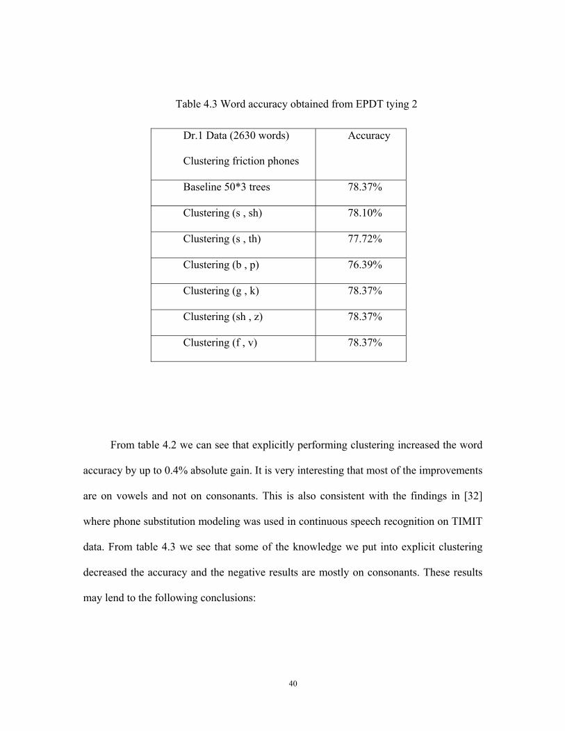
Table 4.3 Word accuracy obtained from EPDT tying 2
Dr.1 Data (2630 words)
Clustering friction phones
Accuracy
Baseline 50*3 trees 78.37%
Clustering (s , sh) 78.10%
Clustering (s , th) 77.72%
Clustering (b , p) 76.39%
Clustering (g , k) 78.37%
Clustering (sh , z) 78.37%
Clustering (f , v) 78.37%
From table 4.2 we can see that explicitly performing clustering increased the word
accuracy by up to 0.4% absolute gain. It is very interesting that most of the improvements
are on vowels and not on consonants. This is also consistent with the findings in [32]
where phone substitution modeling was used in continuous speech recognition on TIMIT
data. From table 4.3 we see that some of the knowledge we put into explicit clustering
decreased the accuracy and the negative results are mostly on consonants. These results
may lend to the following conclusions:
40

1 Consonants are not suitable for explicit tying. This may be due to the wide
diversity that the different consonants have, and the confusions introduced by consonant
clustering may be more than the benefits from pronunciation variations it solves.
2 Vowels are better choices for explicit tying because vowels are more stable.
3 We also observe that in some clustering cases, word accuracy did not change at
all. That happens when the decision tree splits the different phoneme data at the top levels,
and therefore the training data from different center phones never mix up and the
resulting model is exactly the same as the baseline model. This indicates that although
some phones are labeled alike based on the linguistic knowledge source, in
conversational speech data they are still quite different.
In Table 4.4 we evaluated the extreme case of explicit PDT tying. We put the entire
center phone data in the training set to generate 3 Single-Tree PDTs model (3-tree model)
according to 3 emitting states of triphone HMMs. We further separate the consonants and
vowels to 6-tree model because we do not want data sharing between them.
41

Table 4.4 Word accuracy obtained from the extreme case of EPDT tying
Dr.2 Data (5085
words)
Dr.1
(3248)
Dr.2
(5085)
Dr.3
(3988)
Dr.4
(2759)
Dr.5
(6421)
Average2
Baseline
50*3
trees
Accuracy
77.43% 81.26% 82.57% 74.01% 78.71% 79.23%
Model size 1104 2076 1735 1479 1412 1591
3-Tree
Model
Accuracy 75.55% 80.37% 83.95% 73.36% 78.20% 78.76%
Model size 1077 2045 1717 1461 1386 1566
6-Tree
Model
Accuracy 76.57% 81.71% 83.27% 74.63% 78.20% 79.26%
Model size 1064 2035 1708 1436 1386 1556
It is obvious that in our task, the extreme case in explicit PDT tying did not
generate good results in comparison with the 1.8% absolute word accuracy improvement
in [24]. This may be due to the fact that our task is speaker dependent therefore less
pronunciation variations appeared in the speech data.
We also include the baseline and the EPDT model sizes in number of tied states in
Table 4.4, where the EPDTs used the same decision tree construction thresholds in
likelihood gain and data count as the baseline. The sizes for the two extreme cases of the
2 The average word accuracy is already weighted by the word counts for each doctor’s data set shown in the first
row of Table 4.4.
42

EPDT models are smaller than the baseline model. This is due to the increased effect of
phoneme data sharing in EPDT. The 6-Tree model has a smaller size than the 3-tree
model, although the 3-tree model is supposed to have more data sharing. This might be
explained by the greedy process of the decision tree construction. In the 3-tree model, the
root node has a large data diversity due to the full set of phonemes, and therefore the
phonetic questions according to the center phone properties have better chances to be
selected. The result is that some of the phoneme data sharing occurred in the 6-tree model
did not happen in the 3-tree model because the phonemes were separated early at the top
levels of the 3 trees.
4.3 Experimental results for multiple acoustic models based on EPDT
We combined the baseline model with the model from the 3 Single-Consonant-
Trees plus 3 Single-Vowel-Trees (6-Tree model), so that each triphone state will be tied
to two models. The results for five doctors are shown in table 4.5. Here average and max
are two strategies in model combining that are discussed in chapter 3.
Table 4.5 Word accuracy obtained from combining the Baseline and the 6-Tree models
Dr.1
(3248)
Dr.2
(5085)
Dr.3
(3988)
Dr.4
(2759)
Dr.5
(6421)
Average
Baseline 77.43% 81.26% 82.57% 74.01% 78.71% 79.23%
2 Models Average 77.56% 81.79% 83.63% 75.39% 79.66% 80.03%
2 Models Max 77.80% 81.95% 83.63% 75.50% 79.69% 80.13%
43
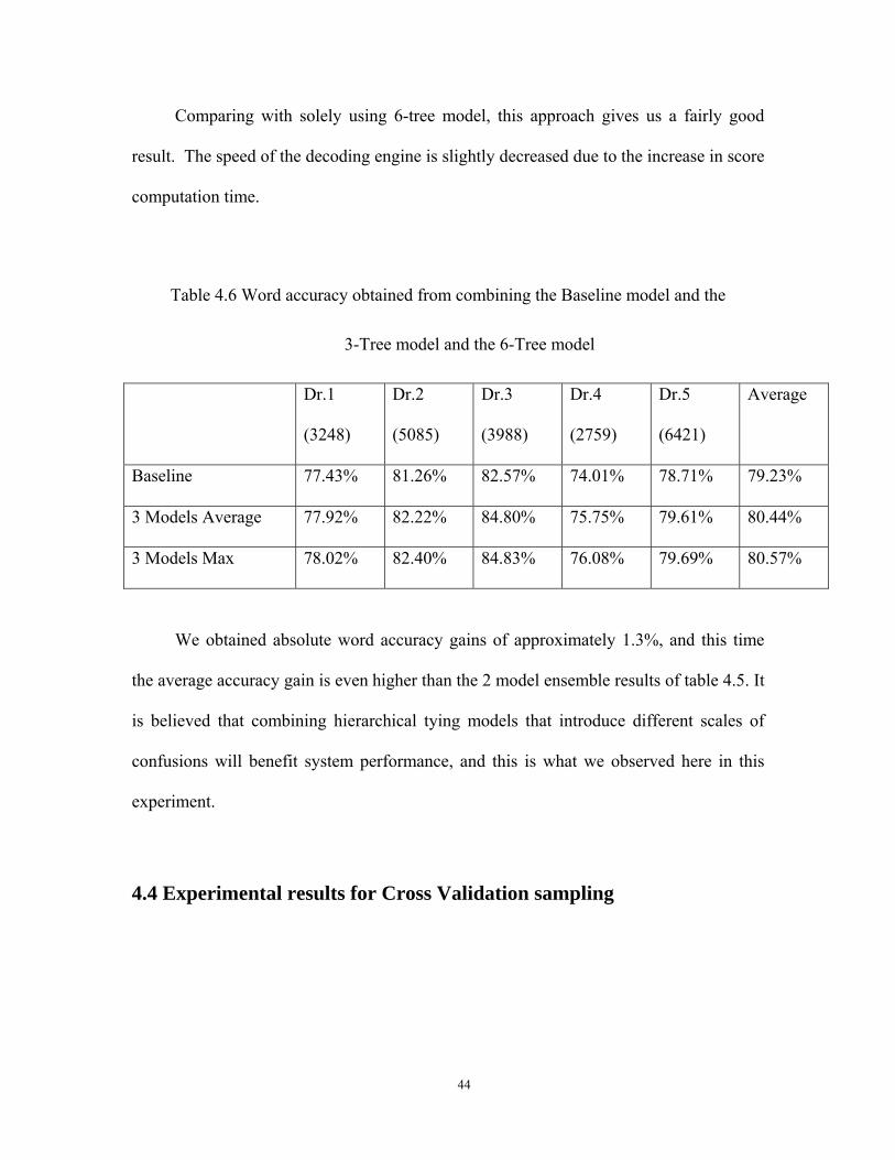
Comparing with solely using 6-tree model, this approach gives us a fairly good
result. The speed of the decoding engine is slightly decreased due to the increase in score
computation time.
Table 4.6 Word accuracy obtained from combining the Baseline model and the
3-Tree model and the 6-Tree model
Dr.1
(3248)
Dr.2
(5085)
Dr.3
(3988)
Dr.4
(2759)
Dr.5
(6421)
Average
Baseline 77.43% 81.26% 82.57% 74.01% 78.71% 79.23%
3 Models Average 77.92% 82.22% 84.80% 75.75% 79.61% 80.44%
3 Models Max 78.02% 82.40% 84.83% 76.08% 79.69% 80.57%
We obtained absolute word accuracy gains of approximately 1.3%, and this time
the average accuracy gain is even higher than the 2 model ensemble results of table 4.5. It
is believed that combining hierarchical tying models that introduce different scales of
confusions will benefit system performance, and this is what we observed here in this
experiment.
4.4 Experimental results for Cross Validation sampling
44

In this experiment we apply Cross Validation (CV) based sampling method for
acoustic modeling and use the models in the current telehealth recognition test with the
Tiger decoding engine, which is described in chapter 3.
Table 4.7 Word accuracy obtained from the Cross Validation based ensemble acoustic
model, Fold size = 10
10 CV Model Dr.1
(3248)
Dr.2
(5085)
Dr.3
(3988)
Dr.4
(2759)
Dr.5
(6421)
Average
Baseline 3 76.69% 81.18% 83.05% 74.48% 78.74% 79.26%
Baseline 77.43% 81.26% 82.57% 74.01% 78.71% 79.23%
Average 79.37% 83.15% 85.26% 76.62% 81.11% 81.52%
Max 79.37% 82.93% 85.32% 76.15% 80.94% 79.67%
n-Best (n=5) 79.34% 83.17% 84.95% 76.44% 81.05% 81.42%
In this experiment we obtained 2.3% absolute word accuracy gain in using the
average combining method. This is a significant improvement in the telehealth captioning
task. For detailed accounts on the significance test on this task, please see [27].
3 This is the baseline that was used in [27]. The difference in baselines may be due to different parameter settings
used in decoding stage.
45

Several issues should be addressed. First is the baseline classifier performance as
we discussed in chapter 3. The results for the individual 10 CV acoustic models are
obtained from the test on Dr.2, shown in Table 4.8.
Table 4.8 The effectiveness of 10-fold CV base classifiers on recognition performance
Dr.2’s data (5085 words) Accuracy
Baseline 81.26%
Model 1 80.77%
Model 2 81.00%
Model 3 79.82%
Model 4 80.69%
Model 5 81.40%
Model 6 81.08%
Model 7 80.93%
Model 8 81.04%
Model 9 80.81%
Model 10 80.96%
10 Model Average 80.85%
10 Model Standard Deviation 0.004119
46
Here we can observe that the performances of most of the base classifiers are lower
than the baseline. It indicates that the training data size and coverage is one of the key
factors in recognition accuracy. However, ensemble classifier also benefited from the
diversity that sampling the training data have generated.
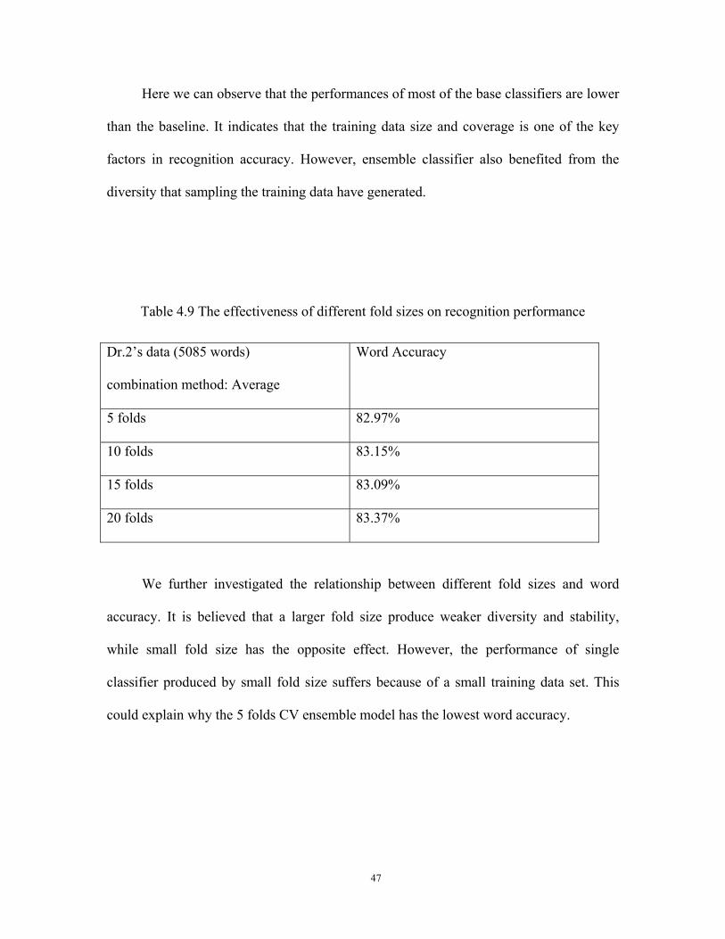
Table 4.9 The effectiveness of different fold sizes on recognition performance
Dr.2’s data (5085 words)
combination method: Average
Word Accuracy
5 folds 82.97%
10 folds 83.15%
15 folds 83.09%
20 folds 83.37%
We further investigated the relationship between different fold sizes and word
accuracy. It is believed that a larger fold size produce weaker diversity and stability,
while small fold size has the opposite effect. However, the performance of single
classifier produced by small fold size suffers because of a small training data set. This
could explain why the 5 folds CV ensemble model has the lowest word accuracy.
47

Table 4.10 The effectiveness of Different mixture sizes on word accuracy performance
Dr.2 ’s Data (5085 words)
combination method:
Average
Single model
Baseline
10 CV
model
8 Mixture Models 79.80% 82.22%
16 Mixture Models 81.26% 83.15%
20 Mixture Models 81.20% 83.37%
24 Mixture Models 80.12% 83.64%
Figure 4.2 The effect of different mixture sizes on word accuracy
48

Here we can observe that mixture size affects the word accuracy differently for the
baseline and the ensemble models. For the baseline model, the accuracy reaches the
highest when the mixture size is equal to 16. It is because low mixture model is not
accurate while high mixture model requires more data to train. For the proposed 10 fold
CV model, we can observe that our approach is superior to the best baseline model, and it
has the property that larger mixture model yields better results. This could be explained
by the variance reduction effect of ensemble models that avoids overfitting.
4.5 Experimental results for Random Sampling
In this experiment we randomly sample the training data without replacement,
which is described in chapter 3. Here we obtained 4 ensemble classifiers with different
number of models and the results are shown in Table 4.11.
49

Table 4.11 Word accuracy obtained from the ensemble models
that are generated through Random Sampling without replacement
Dr.1 Data (2630 words)4 Average Max
Baseline 78.37% 78.37%
10 models 79.06% 79.02%
20 models 79.55% 79.48%
30 models 80.08% 79.86%
50 models 79.89% 79.25%
We can observe that this method also produced a 1.7% absolute increase in word
accuracy over the baseline, when the ensemble size is 30. However, the performance gain
is inferior to the proposed CV based sampling. As we have analyzed, this difference
might be due to the bias in the sampled training data distribution introduced by the
random sampling. The bias should be smaller when the subsets are many, when random
sampling is used to produce infinite number of subsets, the bias will disappear.
4 This dataset is a subset of the Dr.1’s dataset, where the full set has 3248 words.
50

4.6 Experimental results for combining methods
In this experiment we tested several combining methods that are discussed in
chapter 3. Here 10-fold CV was used, and the mixture size was fixed to be 16 per GMD.
Table 4.12: m-best performance
Dr.2 Data (5085 words) Word Accuracy
10-best (Average) 83.15%
7-best 83.17%
5-best 83.17%
3-best 83.28%
1-best (Max) 82.93%
Here, in this test we can see that m = 3 may be a good choice.
Table 4.13: m-Trimmed average performance
10CV Model 10-Trimmed
Average
8-Trimmed
Average
6-Trimmed
Average
4-Trimmed
Average
2-Trimmed
Average
Dr.2 Data
(5085 words)
83.15% 83.21% 82.36% 82.40% 81.95%
In Trimmed average test, 8 trimmed average has the best word accuracy while, 2-
Trimmed average has the lowest word accuracy.
51
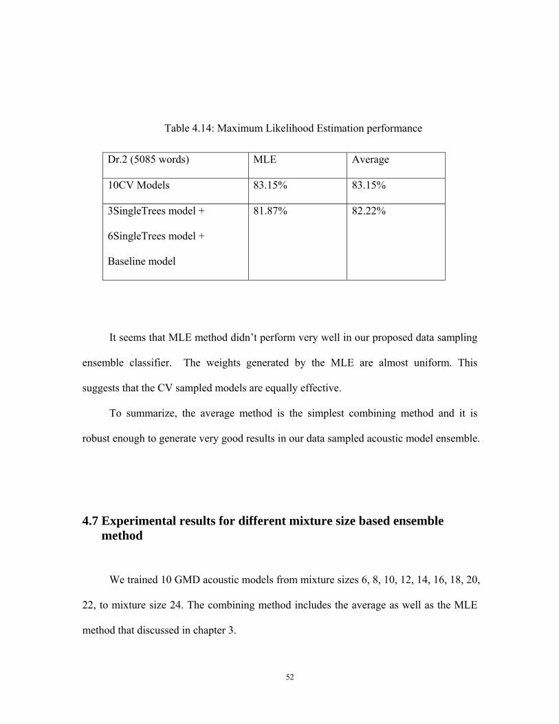
Table 4.14: Maximum Likelihood Estimation performance
Dr.2 (5085 words) MLE Average
10CV Models 83.15% 83.15%
3SingleTrees model +
6SingleTrees model +
Baseline model
81.87% 82.22%
It seems that MLE method didn’t perform very well in our proposed data sampling
ensemble classifier. The weights generated by the MLE are almost uniform. This
suggests that the CV sampled models are equally effective.
To summarize, the average method is the simplest combining method and it is
robust enough to generate very good results in our data sampled acoustic model ensemble.
4.7 Experimental results for different mixture size based ensemble method
We trained 10 GMD acoustic models from mixture sizes 6, 8, 10, 12, 14, 16, 18, 20,
22, to mixture size 24. The combining method includes the average as well as the MLE
method that discussed in chapter 3.
52

Table 4.15 Hierarchical ensemble acoustic model based on 10 models from mixture
size 6 to mixture size 24 on word accuracy test
Dr.2’s data
(5085 words)
Word Accuracy
Baseline 81.26%
Hierarchical ensemble model, Average 82.22%
Hierarchical ensemble model, MLE 82.24%
We obtained an approximately 1% absolute word accuracy improvement
comparing to the baseline. In MLE method, we observed that the weight of a small
mixture sized model is always bigger than the weight of a large mixture sized model.
This indicated that a small mixture sized model has a higher average likelihood score
than a large mixture sized model. It is believed a large mixture sized model is usually
more accurate than small mixture sized model. This indicated that the likelihood score
and the classification accuracy are mismatched. Therefore, confidence measurement
should be considered in the future implementation.
53

Chapter 5
Conclusion
In this thesis, several ensemble methods have been proposed and investigated for
our task of telemedicine large vocabulary conversational speech recognition. The main
contributions of this work include the following two aspects.
1. Explicit Decision Tree tying — by clustering center phone training data based
on linguistic knowledge, we have obtained improved word accuracy in some cases. We
further combined the extreme case of explicit decision tree models with the baseline
model and the word accuracy has been improved notably.
2. Applying data sampling method to obtain an ensemble acoustic model — a
Cross Validation based data sampling method is used which significantly improved the
word accuracy over the baseline model.
Ensemble modeling is a very promising direction in ASR area. Potential future
extensions to this work are the following:
1. Ensemble classifier compromises the speed of decoding search. One possible
way to address this problem is to perform model reduction by performing clustering on
base classifiers, which has been shown effective in [27]. We can also apply parallel
computing in the decoding engine to compute the scores simultaneously from different
models. Or we can integrate a second pass rescoring by using the ensemble classifier with
the first pass decoding by using the simple baseline classifier to decrease the computation
load in the first pass.
54

2. Ensemble acoustic models in general generates a higher average acoustic score
per speech frame, since it matches better to input data and is more stable. Therefore the
parameters of language model scale and word penalty that are tuned to balance language
model and acoustic model scores should be retuned. How to successfully retune the
parameters automatically based on the new ensemble classifier is worth investigating.
3. There are still many data sampling approaches, such as bootstrapping, over
sampling, as well as discriminative boosting or ada-boosting methods that are worth
investigating on our task as well as on other ASR tasks.
55

Reference
[1] L. R. Rabiner, and Bing-Hwang Juang, Fundamentals of speech recognition, Prentice
Hall Press, 1993.
[2] Robert V. Hogg, Allen T. Craig, “Introduction to Mathematical Statistics,”
Prentice Hall Press, 1995.
[3] GD Forney Jr, “The viterbi algorithm”, proceedings of IEEE, pp 268-278 1973
[4] B. S. Atal, and M. R. Schroeder, “Predictive coding of speech signals,” Proc.
AFCRL/IEEE conference on speech communication and processing, pp. 360-361, 1967
[5] H. Hermansky, “Perceptual Linear Predictive (PLP) analysis of speech,” J. Acoustic
Society of America, 87, pp. 1738-1752, 1990.
[6] P. Mermelstein, “Distance measures for speech recognition, psychological and
instrumental,” Pattern Recognition and Artificial Intelligence, C. H. Chen, Ed. New York:
Academic, pp. 374-388, 1976.
[7] S. Furui, “Speaker Independent Isolated Word Recognition Using Dynamic Features
of Speech Spectrum,” IEEE Transactions on Acoustic, Speech and Signal Processing, vol.
34, no. 1, pp. 52~59, 1986.
[8] N. Kumar, and A. G. Andreou, “Heteroscedastic Discriminant Analysis and Reduced
Rank HMMs for Improved Speech Recognition,” Speech Communication, vol. 26, pp.
283-297, 1998.
[9] A. Hyvarinen, and E. Oja, “Independent Component Analysis: a Tutorial,”
http://www.cis.hut.fi/aapo/papers/IJCNN99_tutorialweb/
[10] M. Tomita, “An efficient augmented-context-free parsing algorithm,” Computer
Linguistics, 13 (1-2), pp. 31-46, 1987.
56

[11] F. Jelinek, “Up from trigrams! - the struggle for improved language models,” Proc.
of Eurospeech, pp. 1037-1040, 1991.
[13] HTK Toolkit, http://htk.eng.cam.ac.uk.
[14] Richard Bellman, “Dynamic Programming”, Science Vol 153, pp 34-37, 1966
[15] Mari Ostendorf, Izhak Shafran and Rebecca Bates, “Prosody Models for
Conversational Speech Recognition”, Proc. of the 2nd Plenary Meeting and Symposium
on Prosody and Speech Processing, pp. 147-154, 2003.
[16] S. Seneff, “The use of subword linguistic modeling for multiple tasks in speech
recognition,” Speech Commun., vol. 42, pp. 373–390, Apr.2004.
[17] D. Jurafsky, W.Ward, J. Zhang, K. Herold, X. Yu, and S. Zhang, “What kind of
pronunciation variation is hard for triphones to model?,” in Proc. 2001 IEEE Int. Conf.
Acoust., Speech, Signal Process., Salt Lake City, UT, May 2001, pp. 577–580.
[18] S. Greenberg, “Speaking in shorthand—A syllable-centric perspective for
understanding pronunciation variation,” Speech Commun., vol. 29, no. 2–4, pp. 159–176,
Nov. 1999.
[19] M. Riley, B. Byrne, M. Finke, S. Khudanpur, A. Ljolje, J. McDonough, H. Nock, M.
Saraclar, C. Wooters, and G. Zavaliagkos, “Stochastic pronunciation modeling from
hand-labeled phonetic corpra,” Speech Commun., vol. 29, pp. 209–224, Nov. 1999.
[20] J. Xue, Y. Zhao, “Novel Lookahead Decision Tree State Tying for Acoustic
Modeling” Proc. ICASSP, pp 1133-1136, 2007
[21] W. Reichl and W. Chou, “Robust decision tree state tying for continuous speech
recognition,” IEEE Trans. Speech Audio Process., vol. 8, no. 5, pp. 555–566, Sep. 2000.
57

[22] I. Shafran and M. Ostendorf, “Acoustic model clustering based on syllable
structure,” Comput. Speech Lang., vol. 17, no. 4, pp. 311–328, 2003.
[23] Jurafsky et al., 2001 Jurafsky, D., et al., 2001. What kind of pronunciation variation
is hard for triphones to model? In: Proc. 2001 IEEE International Conference on
Acoustics, Speech, and Signal Processing, Salt Lake City, Utah. IEEE, Piscataway, New
Jersey, pp. 577–580.
[24] Yu H. and Schultz T., “Enhanced tree clustering with single pronunciation
dictionary for conversational speech recognition,” Eurospeech, pp. 1869-1872, 2003.
[25] Greenberg, S., The Switchboard transcription project. LVCSR Summer Research
Workshop. Johns Hopkins University, Baltimore, MD, 1996
[26] J.G.Fiscus, “A post-processing system to yield reduced word error rates: Recognizer
Output Voting Error Reduction (ROVER), Proc. IEEE ASRU Workshop, pp. 347-352,
1997.
[27] J. Xue, Y. Zhao, “Random Forests of Phonetic Decision Trees for Acoustic
Modeling in Conversational Speech Recognition” IEEE Transactions on Speech and
Audio Processing, vol.16, iss. 3, pp.519-528, 2008
[28] Samuel Chindaro, Konstantinos Sirlantzis, Michael Fairhurst, “Modelling Multiple-
Classifier Relationships using Bayesian Belief Networks” MSC workshop proceedings,
2007
[29] Y. Zhao, X. Zhang, R.-S. Hu, J. Xue, X. Li, L. Che, R. Hu, and L. Schopp,, “An
Automatic Captioning System for Telemedicine,” Proc. ICASSP, pp. I-957 – I-960, 2006.
58

59
[30] X. Zhang, Y. Zhao, and L. Schopp, “A novel method of language modeling for
automatic captioning in TC video teleconferencing,” IEEE Trans. Information
Technology in Biomedicine, vol.11,pp. 332-337, 2007.
[31] X. Li and Y. Zhao, “A fast and memory-efficient N-gram language model lookup
method for large vocabulary continuous speech recognition,” Computer Speech &
Language, vol. 21, iss. 1, pp. 1-25, 2007.
[32] Y. Zhao, “Hierarchical mixture models and phonological rules in open-vocabulary
speech recognition,” Euro speech, pp. 1586-1590, 1995
[33] Albert Hung-Ren Ko, etal. “A new HMM- Based ensemble generation method for
numerical recognition,” MCS workshop, pp. 52-61, 2007