Embed Size (px)
Citation preview
ENHANCING A DECISIONSUPPORT TOOL WITHSENSITIVITY ANALYSIS
A dissertation submitted to the University of Manchester for the
degree of Master of Science
in the Faculty of Engineering and Physical Sciences
2012
By
Renzo Cristian Bertuzzi Leonelli
School of Computer Science

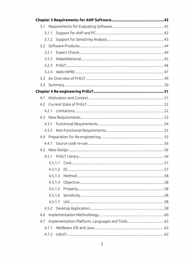
Table of Contents
List of Tables................................................................................................................. 7
List of Figures................................................................................................................ 8
List of Algorithms.........................................................................................................9
List of Acronyms.........................................................................................................10
Abstract........................................................................................................................ 11
Declaration.................................................................................................................. 12
Intellectual Property Statement...........................................................................13
Acknowledgements...................................................................................................14
Chapter 1 Introduction.............................................................................................15
1.1 Project Context...............................................................................................15
1.2 Aims and Objectives.......................................................................................17
1.3 Contributions.................................................................................................. 18
1.3.1 Implementation of three SA algorithms.............................................18
1.3.2 Re-engineering and enhancing PriEsT with SA...................................18
1.3.3 Method for selecting a single solution for a PC matrix.....................19
1.3.4 Implementation of a web version of PriEsT........................................19
1.3.5 Implementation of a mobile version of PriEsT...................................19
1.4 Dissertation Structure....................................................................................19
Chapter 2 Project Background................................................................................21
2.1 Multi-Criteria Decision Making......................................................................21
2.2 Analytic Hierarchy Process............................................................................22
2.3 Pairwise Comparison (PC) Method...............................................................25
2.4 Elicitation Methods........................................................................................27
2.5 Error Measures................................................................................................28
2.6 An Illustrative Example..................................................................................28
2.7 Sensitivity Analysis..........................................................................................32
2.7.1 Numerical Incremental Analysis............................................................33
2.7.2 Probabilistic Simulations........................................................................35
2.7.3 Mathematical Models.............................................................................38
2.8 Summary.......................................................................................................... 41
2
Chapter 3 Requirements for AHP Software........................................................42
3.1 Requirements for Evaluating Software.......................................................42
3.1.1 Support for AHP and PC........................................................................42
3.1.2 Support for Sensitivity Analysis............................................................43
3.2 Software Products..........................................................................................44
3.2.1 Expert Choice..........................................................................................44
3.2.2 MakeItRational........................................................................................45
3.2.3 PriEsT........................................................................................................ 46
3.2.4 Web-HIPRE...............................................................................................47
3.3 An Overview of PriEsT....................................................................................49
3.4 Summary.......................................................................................................... 50
Chapter 4 Re-engineering PriEsT...........................................................................51
4.1 Motivation and Context.................................................................................51
4.2 Current State of PriEsT..................................................................................52
4.2.1 Limitations...............................................................................................52
4.3 New Requirements.........................................................................................53
4.3.1 Functional Requirements......................................................................54
4.3.2 Non-Functional Requirements..............................................................55
4.4 Preparation for Re-engineering...................................................................55
4.4.1 Source code re-use.................................................................................56
4.5 New Design...................................................................................................... 56
4.5.1 PriEsT Library...........................................................................................56
4.5.1.1 Core...................................................................................................57
4.5.1.2 IO....................................................................................................... 57
4.5.1.3 Method.............................................................................................58
4.5.1.4 Objective..........................................................................................58
4.5.1.5 Property...........................................................................................58
4.5.1.6 Sensitivity.........................................................................................58
4.5.1.7 Util..................................................................................................... 58
4.5.2 Desktop Application...............................................................................58
4.6 Implementation Methodology.....................................................................60
4.7 Implementation Platform, Languages and Tools.......................................63
4.7.1 NetBeans IDE and Java..........................................................................63
4.7.2 LWUIT....................................................................................................... 63
3
4.7.3 Sun Java Wireless Toolkit.......................................................................63
4.7.4 Android SDK............................................................................................63
4.7.5 Retrotranslator.......................................................................................64
4.8 Summary.......................................................................................................... 64
Chapter 5 Sensitivity Analysis Implementation.................................................65
5.1 One-at-a-time.................................................................................................. 65
5.1.1 Algorithm.................................................................................................65
5.1.2 Implementation in PriEsT......................................................................66
5.1.3 Advantages..............................................................................................67
5.1.4 Limitations...............................................................................................68
5.2 Probabilistic Simulation.................................................................................69
5.2.1 Algorithm.................................................................................................69
5.2.1.1 Uniform weight generator............................................................71
5.2.1.2 Gamma weight generator.............................................................72
5.2.1.3 Triangular weight generator.........................................................72
5.2.2 Implementation in PriEsT......................................................................73
5.2.3 Advantages..............................................................................................74
5.2.4 Limitations...............................................................................................75
5.3 Mathematical Modelling................................................................................76
5.3.1 Algorithm.................................................................................................76
5.3.1.1 Top Level Algorithm.......................................................................77
5.3.1.2 Middle Level Algorithm..................................................................78
5.3.1.3 Bottom Level Algorithm................................................................79
5.3.1.4 Sensitivity Coefficients...................................................................83
5.3.2 Implementation in PriEsT......................................................................83
5.3.2.1 Uni-dimensional Transformation..................................................84
5.3.2.2 Two-dimensional Transformation.................................................86
5.3.2.3 Three-dimensional Transformation..............................................86
5.3.2.4 Multi-dimensional Transformation...............................................87
5.3.2.5 Sensitivity Coefficients and Rank Reversal.................................87
5.3.2.6 Most Sensitive Decision Element.................................................88
5.3.3 Advantages..............................................................................................88
5.3.4 Limitations...............................................................................................89
5.4 Select a Single Solution from PrInT..............................................................89
4
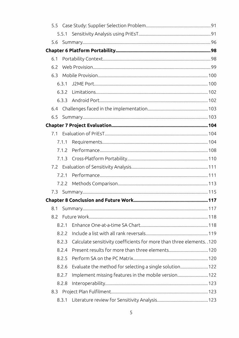
5.5 Case Study: Supplier Selection Problem.....................................................91
5.5.1 Sensitivity Analysis using PriEsT............................................................91
5.6 Summary.......................................................................................................... 96
Chapter 6 Platform Portability...............................................................................98
6.1 Portability Context.........................................................................................98
6.2 Web Provision................................................................................................. 99
6.3 Mobile Provision...........................................................................................100
6.3.1 J2ME Port..............................................................................................100
6.3.2 Limitations.............................................................................................102
6.3.3 Android Port..........................................................................................102
6.4 Challenges faced in the implementation..................................................103
6.5 Summary........................................................................................................103
Chapter 7 Project Evaluation................................................................................104
7.1 Evaluation of PriEsT.....................................................................................104
7.1.1 Requirements........................................................................................104
7.1.2 Performance..........................................................................................108
7.1.3 Cross-Platform Portability...................................................................110
7.2 Evaluation of Sensitivity Analysis...............................................................111
7.2.1 Performance..........................................................................................111
7.2.2 Methods Comparison...........................................................................113
7.3 Summary........................................................................................................115
Chapter 8 Conclusion and Future Work.............................................................117
8.1 Summary........................................................................................................117
8.2 Future Work..................................................................................................118
8.2.1 Enhance One-at-a-time SA Chart........................................................118
8.2.2 Include a list with all rank reversals....................................................119
8.2.3 Calculate sensitivity coefficients for more than three elements. .120
8.2.4 Present results for more than three elements................................120
8.2.5 Perform SA on the PC Matrix..............................................................120
8.2.6 Evaluate the method for selecting a single solution.......................122
8.2.7 Implement missing features in the mobile version.........................122
8.2.8 Interoperability.....................................................................................123
8.3 Project Plan Fulfilment................................................................................123
8.3.1 Literature review for Sensitivity Analysis..........................................123
5

8.3.2 Decision Support Tools Comparison..................................................124
8.3.3 Re-engineering PriEsT and SA implementation...............................124
8.3.4 Platform provision................................................................................124
8.3.5 Project Evaluation................................................................................124
8.4 Conclusion.....................................................................................................125
List of References....................................................................................................126
Appendix A UML Design.........................................................................................132
Appendix B Unit Tests............................................................................................134
Appendix C PriEsT Library Usage........................................................................137
Appendix D Application Screen-shots................................................................139
Appendix E Project Gantt Chart..........................................................................143
Word Count: 29780
6

List of Tables
Table 2.1. Scale of Relative Importance (Saaty, 1980)............................................26
Table 2.2. Pairwise matrix for the goal......................................................................30
Table 2.3. Pairwise matrix for Amenities...................................................................30
Table 2.4. Pairwise matrix for alternatives under criterion Price..........................30
Table 2.5. Pairwise matrix for alternatives under criterion MPG...........................31
Table 2.6. Pairwise matrix for alternatives under criterion Prestige....................31
Table 2.7. Pairwise matrix for alternatives under criterion Comfort....................31
Table 2.8. Pairwise matrix for alternatives under criterion Style..........................31
Table 3.1. Expert Choice Software Evaluation.........................................................45
Table 3.2. MakeItRational Software Evaluation.......................................................46
Table 3.3. PriEsT Software Evaluation.......................................................................47
Table 3.4. Web-HIPRE Software Evaluation..............................................................48
Table 5.1. Statistical Measures in Probabilistic Simulation SA...............................71
Table 5.2. PrInT Solutions............................................................................................90
Table 5.3. Sensitivity coefficients...............................................................................96
Table 5.4. Ranking of suppliers with different weight combinations...................96
Table 7.1. Traceability matrix for new requirements............................................106
Table 7.2. PriEsT v2 Software Evaluation................................................................107
7
List of Figures
Figure 2.1. A hierarchy model in AHP........................................................................24
Figure 2.2. Car selection example..............................................................................29
Figure 2.3. Numerical Incremental Sensitivity Analysis...........................................34
Figure 2.4. Box-plot Chart Presenting Simulation Results.....................................36
Figure 2.5. Ranking of Alternatives in the Weight Space........................................40
Figure 4.1. Old MVC Architecture of PriEsT..............................................................53
Figure 4.2. PriEsT Library Design................................................................................57
Figure 4.3. MVC Architecture......................................................................................59
Figure 4.4. PriEsT UI...................................................................................................... 61
Figure 4.5. Implementation Steps..............................................................................62
Figure 5.1. On-at-a-time Sensitivity Analysis.............................................................67
Figure 5.2. Gamma and Triangular Distribution.......................................................70
Figure 5.3. Probabilistic Simulation Sensitivity Analysis..........................................74
Figure 5.4. Hierarchy Tree for Mathematical SA......................................................77
Figure 5.5. Allowable range of perturbations (Chen, 2008)...................................82
Figure 5.6. Uni-dimensional Projection.....................................................................85
Figure 5.7. Two-dimensional Projection....................................................................85
Figure 5.8. Three-Dimensional Projection................................................................86
Figure 5.9. AHP model for supplier selection...........................................................92
Figure 5.10. Ranking of alternatives using probabilistic simulation.....................93
Figure 5.11. Ranking of alternatives using one-at-a-time analysis........................94
Figure 5.12. Ranking of alternatives using the mathematical SA .........................95
Figure 6.1. Dependency of PriEsT Implementations...............................................99
Figure 6.2. Package Diagram for PriEsT Mobile.....................................................100
Figure 6.3. PriEsT Mobile...........................................................................................101
Figure 7.1. Start-up time............................................................................................108
Figure 7.2. Performance comparison......................................................................109
Figure 7.3. Performance of elicitation methods for PriEsT Mobile....................110
Figure 7.4. Computation time for SA methods......................................................112
Figure 7.5. SA Method Comparison.........................................................................114
8

List of Algorithms
Algorithm 5.1. On-at-a-time SA and rank reversals..................................................66
Algorithm 5.2. Probabilistic simulation algorithm...................................................69
Algorithm 5.3. Uniform weight generator................................................................71
Algorithm 5.4. Triangular weight generator.............................................................72
Algorithm 5.5 Allowable region for top level criteria.............................................78
Algorithm 5.6 Allowable region for middle level criteria.......................................79
Algorithm 5.7 Allowable region for bottom level alternatives..............................81
Algorithm 5.8 Select a single solution from PrInT...................................................90
9

List of Acronyms
AHP Analytic Hierarchy Process
CI Consistency Index
CR Consistency Ratio
DM Decision Maker
EV Eigenvector
GM Geometric Mean
GDM Group Decision Making
IAHP Interval AHP
J2ME Java 2 Micro Edition
JIT Just In Time Compiler
JVM Java Virtual Machine
MCDM Multi-Criteria Decision Making
MIDlet MIDP Application
MIDP Mobile Information Device Profile
MVC Model View Controller
NV Number of Violations
OAT One At a Time
OPSC Operating Point Sensitivity Coefficient
PC Pairwise Comparison
PrInT Prioritisation using Indirect Judgements
RR% Rank Reversal Probability
SA Sensitivity Analysis
SC Sensitivity Coefficient
TD Total Deviation
TD2 Total Deviation Using Indirect Judgements
TDD Test Driven Development
TSC Total Sensitivity Coefficient
WSM Weighted Sum Model
10

Abstract
With the increased speed and complexity of today's world, and the ever
increasing amount of data available, a decision support system is of critical
importance.
Multi-Criteria Decision Making (MCDM) enables decision makers to make a
decision considering several alternatives and multiple criteria of evaluation. The
Analytic Hierarchy Process (AHP) is an area of research in MCDM where the
problem is decomposed into a hierarchical model in order to rank the
alternatives. Sensitivity analysis (SA) is a technique that determines the effects
of changes in input values on a model results, hence, performing an SA on the
results of a decision problem may provide valuable information to the decision
maker about the robustness of the solution.
This work investigates various methods to carry out SA on AHP models. In
addition, a framework for evaluating software in terms of AHP features and SA
support is developed and a number of commercial and academic software tools
are analysed using this framework. The result from this analysis shows that
despite the existence of several approaches to performing SA, available
software tools only provide a basic form of SA. As a consequence, based on the
framework analysis, an appropriate tool is enhanced to include an SA module.
In summary, the implementation of additional features and improvements
involves a re-engineering process of the AHP tool. Because of the re-
engineering activity, the performance of the re-designed tool has been
improved by a factor of two compared to the original version. Additionally, as a
consequence of this re-engineering, the enhanced tool is also made available on
web and mobile platforms. Further, a major challenge in the area is the problem
of selecting a single solution from a set of non-dominated solutions generated
from the input judgements; to make progress towards this, a selection method
is developed using one of the implemented SA algorithms.
11

Declaration
No portion of the work referred to in this dissertation has been
submitted in support of an application for another degree or
qualification of this or any other university or other institute of
learning.
12

Intellectual Property Statement
i. The author of this dissertation (including any appendices and/or
schedules to this dissertation) owns certain copyright or related rights in
it (the “Copyright”) and s/he has given The University of Manchester
certain rights to use such Copyright, including for administrative
purposes.
ii. Copies of this dissertation, either in full or in extracts and whether in
hard or electronic copy, may be made only in accordance with the
Copyright, Designs and Patents Act 1988 (as amended) and regulations
issued under it or, where appropriate, in accordance with licensing
agreements which the University has entered into. This page must form
part of any such copies made.
iii. The ownership of certain Copyright, patents, designs, trade marks and
other intellectual property (the “Intellectual Property”) and any
reproductions of copyright works in the dissertation, for example graphs
and tables (“Reproductions”), which may be described in this
dissertation, may not be owned by the author and may be owned by
third parties. Such Intellectual Property and Reproductions cannot and
must not be made available for use without the prior written permission
of the owner(s) of the relevant Intellectual Property and/or
Reproductions.
iv. Further information on the conditions under which disclosure,
publication and commercialisation of this dissertation, the Copyright and
any Intellectual Property and/or Reproductions described in it may take
place is available in the University IP Policy (see http://documents.
manchester.ac.uk/display.aspx?DocID=487), in any relevant
Dissertation restriction declarations deposited in the University Library,
The University Library’s regulations (see http://www.manchester.
ac.uk/library/aboutus/regulations) and in The University’s
Guidance for the Presentation of Dissertations.
13

Acknowledgements
I express my sincere appreciation to my supervisor professor John Keane. He
has helped me with wise advice, invaluable support and contributions to make
this dissertation possible.
I also wish to thank the Chilean Government and Conicyt for the wonderful
scholarship program “Becas Chile” that allowed me to be here to pursue this
great and exciting challenge.
14
Chapter 1
Introduction
1.1 Project Context
Everyone has to make decisions, all the time. Some decisions are very simple
and have such a small impact that they can be taken without much analysis. In
contrast, there are complex decisions with a significant impact that have to be
taken with as much information, analysis and reflection as possible to decide on
the possible alternatives. Managerial decisions may have a significant impact on
the performance and success of companies. For example, Campbell et al.
(Campbell, 2009) and Janis (Janis, 1972) have identified examples where clearly
very wrong decisions have been made. With the increased speed and
complexity of today's world and the ever increasing amount of data available,
decision support is of critical importance.
Decision making is a structured process that formalises the steps involved in
making decisions. Multi-Criteria Decision Making (MCDM) is a discipline that
enables decision makers to make a decision considering several alternatives and
multiple criteria of evaluation. MCDM has become so attractive that several
books, thousands of articles and many scientific journals are dedicated to the
subject (Figeroa, 2005).
The Analytic Hierarchy Process (AHP) (Saaty, 2008) is an area of research in
MCDM where the problem is decomposed into a hierarchical model,
represented as a tree. The top element of the hierarchy represents the overall
goal, intermediate nodes correspond to the different criteria and the leaves of
the hierarchy tree are the alternatives. The relative importance of the
alternatives and criteria is assessed by using the Pairwise Comparison (PC)
method. Once all nodes in the hierarchy tree are evaluated, then the
aggregated importance of the alternatives is calculated and a solution or
ranking is obtained, known as the preference vector .
15

Chapter 1. Introduction 16
To assess the importance of alternatives and criteria using PC, only two
elements are compared at a time. The value assigned to this comparison, or
judgement, may have an objective or subjective origin. In either case, the
judgements represent the direction of preference between the two elements
and the strength of this relation. For each criterion a matrix is formed with the
judgements and an elicitation method is used to obtain the preference vector
for this matrix containing the weights of each element.
Often, decision makers (DM) are not completely confident about their
judgements they assign to each comparison; the judgements may be too
subjective or may come from a group decision where members may have
different opinions about each criterion (Erkut, 1991). In such cases, it is
desirable to run a sensitivity analysis (SA) on the results to analyse how sensitive
the solution is to changes in input data. SA is a technique that determines the
effects of changes in input values on a model's results. In this way, SA is a
powerful tool to assess how the preference vector is affected by changes in the
PC judgements or in the weights of the elements. SA may be useful in providing
information equally important to the solution of the problem (Chen, 2008) such
as analysis of the robustness of the recommended solution, identification of
critical elements in the model and help to answer “what if” questions.
Several software tools provide support for both AHP and some level of SA;
some have been in the market for many years, e.g. Web-HIPRE (Mustajoki,
2000), while others have been developed recently, e.g. MakeItRational
(MakeItRational, 2012). Given the importance and popularity of the AHP field
and the usefulness of SA, various approaches in the literature for performing SA
will be analysed. Based on these analyses, a framework of desirable features for
AHP software will be constructed and various software tools will be assessed
according to this framework. The objective of this framework is to assess the
potential of AHP software to deliver a set of important features necessary to
provide a satisfactory solution to a decision problem, and identify potential
improvements that may help the DM to make more robust decisions.
The framework has identified PriEsT (Priority Estimation Tool), an MCDM AHP
Chapter 1. Introduction 17
tool developed at the University of Manchester ((Siraj, 2011), (Siraj, 2012a))
available for Linux and Windows, as the best current offering despite it not
offering support for SA. To implement additional SA features in PriEsT, a
process of re-engineering is important to analyse the application and to
improve its modularity, code readability and reduce the time needed to add
new functionalities (Sommerville, 2000). As a consequence of this re-
engineering, the enhanced PriEsT tool will also be made available on web and
mobile platforms.
1.2 Aims and Objectives
The aims and objectives of this project were to:
1. Investigate how to perform sensitivity analysis in the context of AHP and
the different methods that are available in the literature.
2. Perform a survey of the software tools that support AHP and SA, and
develop a framework that enables comparison in terms of desirable
features or requirements.
3. Select an appropriate MCDM tool for development – PriEsT has been
selected.
4. Improve PriEsT with support for additional desirable features (SA, and
web and mobile deployment).
The general aim of this research and implementation project was to investigate
methods to perform SA in AHP. Following this, PriEsT was analysed, re-
engineered as appropriate, and enhanced by including a module for SA. As a
consequence of this re-engineering various further enhancements were
identified and developed, such as additional platform availability.
To accomplish the goal of the project the following objectives were defined:
• Explore AHP and SA methods. Review the literature to identify the
existing methods to perform SA.
• Re-engineer and re-structure PriEsT in a modular way. Create a library
Chapter 1. Introduction 18
with the AHP functionalities and SA.
• Following this re-engineering, develop further enhancements that will
provide additional platform availability:
◦ a web version of PriEsT as a Java Applet.
◦ a mobile version of PriEsT as a J2ME MIDlet1.
• Carry out an evaluation to measure the performance and efficacy of SA
methods and performance of platform-specific versions of PriEsT.
1.3 Contributions
1.3.1 Implementation of three SA algorithms
Three SA algorithms are studied and implemented: one-at-a-time, probabilistic
simulations and mathematical modelling. Implementation details are given for
each algorithm; in addition, performance tests are executed and the methods
are compared to evaluate their efficacy in analysing decision problems. Based
on our literature analysis and evaluation framework, the enhanced PriEsT tool
would appear to be the only one that has three approaches to SA.
1.3.2 Re-engineering and enhancing PriEsT with SA.
The PriEsT tool is re-engineered and, as a consequence, an open source Java
library is developed, named the PriEsT library. This library contains a set of
functionalities to work with AHP problems and SA.
In addition, a new platform-independent version of PriEsT is designed and
implemented using Java. This application uses the PriEsT library as the core and
allows users to work with decision problems and perform the three different
types of SA.
Because of the re-engineering activity, the performance of the re-designed tool
1 A MIDlet is an application written in Java Micro Edition targeted to run on mobile devices
using the MIDP profile.
Chapter 1. Introduction 19
has also been improved by a factor of two compared to the original version.
1.3.3 Method for selecting a single solution for a PC matrix
A major challenge in the AHP and PC area is the problem of selecting a single
solution from a set of non-dominated solutions generated from the input
judgements; to make progress towards this, a novel selection method has been
developed to evaluate and select a single solution using the mathematical
modelling algorithm for performing SA.
1.3.4 Implementation of a web version of PriEsT
A web version of PriEsT is implemented as a Java Applet. This web application is
built on top of the desktop application and the PriEsT library and allows PriEsT
to run on any web-browser that supports Java without the need to download or
install any software.
1.3.5 Implementation of a mobile version of PriEsT
Two mobile versions of PriEsT are developed: one for the J2ME platform and
one for the Android platform. These applications are compatible with the
desktop and web version, so problems files created with any version can be
interchanged among applications.
1.4 Dissertation Structure
This dissertation contains eight chapters. The present chapter has introduced
the project's context, aims and objectives and has presented the contributions
of the work.
Chapter 2 reviews the multi-criteria decision making field. Relevant material
about the Analytical Hierarchy Process (AHP) and pairwise comparison (PC) is
given. The chapter ends with an examination of the techniques to perform
sensitivity analysis (SA) in AHP models.
Chapter 3 presents a survey of several decision support tools and performs a

Chapter 1. Introduction 20
comparison to evaluate which tools support the features presented in Chapter
2. As the PriEsT tool obtained the highest score in the evaluation, it is selected
to be enhanced by including the SA techniques identified in Chapter 2.
In order to enhance PriEsT, a re-engineering process is carried out as discussed
in Chapter 4. The motivations for the re-engineering process are laid out; an
analysis of the architecture and source code is presented; new requirements are
introduced; finally, a new design, implementation methodology and tools are
presented.
Chapter 5 discusses the design and implementation of three different SA
methods. Details about the implementation along with the main advantages
and limitations of each method are presented. The chapter concludes with the
presentation of a case study to demonstrate the use of the SA methods.
The advantages of the re-engineering process allows the creation of a web and
mobile version of the application, which are presented in Chapter 6.
Architecture design and implementation details are covered. In addition, the
challenges faced during the implementation process are considered.
Chapter 7 presents the evaluations and system testing performed in the
project. A traceability matrix is presented to evaluate the fulfilment of
requirements and performance tests are discussed for the desktop and mobile
applications. The chapter concludes by presenting the results of specific
performance tests to evaluate the SA algorithms.
Chapter 8 concludes the project. A summary of the project and its main
achievements are presented, followed by several suggestions for future work. A
brief discussion is presented reviewing the project plan and how each objective
was achieved. Finally, the dissertation is finalised with the presentation of
concluding remarks.
Supplementary materials that are referenced in the dissertation are given in the
appendices.

Chapter 2
Project Background
This chapter presents relevant background material. First, an introduction to
the Multi-Criteria Decision Making field is given. Then, the Analytic Hierarchy
Process and the Pairwise Comparison methods are described. Next, different
techniques for performing sensitivity analysis are discussed. Finally, desirable
features of AHP software and existing tools are considered.
2.1 Multi-Criteria Decision Making
Multi-Criteria Decision Making (MCDM) is an area of Operational Research that
supports the process of decision making. In MCDM, the goal is to rank different
alternatives considering multiple, often conflicting, criteria. For example,
consider buying a new car, some of the criteria to consider and evaluate are
cost, fuel consumption, safety, capacity and style. After evaluating a list of
possible cars against these criteria, a ranking of cars can be obtained and the
most appropriate choice can be selected.
For an alternative to be judged by a criterion, a scale of possible values must be
defined for the criterion. A scale is defined by the direction (cost or benefit) and
the magnitude of the values. In addition, different types of criteria may be used
including measurable, ordinal, probabilistic or fuzzy criteria (Jacquet-Lagrèze,
2001).
To find the highest scoring alternative, the DM must evaluate all possible
choices against each criterion. Then a prioritisation method is applied to
aggregate all judgements and create a ranking of the alternatives. Finally, the
DM uses this information as a recommendation to select one of the alternatives
according to his/her requirements and preferences.
The MCDM methodology is a process that includes four main steps beginning
with the definition of the decision problem and ending with the selection of an
alternative (Jacquet-Lagrèze, 2001). The steps are as follows:
21
Chapter 2. Project Background 22
1. Structuring the decision problem: the DM establishes the problem
and the set of possible alternatives to consider.
2. Modelling the criteria: the criteria and the way to measure the
alternatives for each criterion are defined.
3. Aggregating the preferences: each alternative is judged against
each criterion and an aggregation method is used to derive the ranking
of alternatives.
4. Recommendations: recommendations are given to the DM based on
the results from the previous step. The DM selects one of the
alternatives.
There exist several prioritisation methods2 (Triantaphyllou, 2000) that
aggregate the preferences in step 3 and different methods may yield different
results. Although studies (Guitoni, 1998) have compared different methods and
introduced frameworks for selecting the most appropriate depending on the
problem, according to a study from Wallenius et al. (Wallenius, 2008) in 2008,
the most popular method in the literature since the 1970s has been the
Analytical Hierarchy Process (AHP). The AHP method is described in the next
section.
2.2 Analytic Hierarchy Process
AHP is a method of prioritisation that enable DMs to evaluate the relative
importance of objective and subjective alternatives and criteria by using the
pairwise comparison technique. It was introduced by Saaty in 1980 (Saaty, 1980)
and has proven very popular worldwide since its creation (Wallenius, 2008).
To apply the AHP method a decision problem must be decomposed into four
steps (Saaty, 2008):
2 The most popular methods are: weighted sum model (WSM), weighted product model
(WPM), analytic hierarchy process (AHP) (Saaty, 1980), ELECTRE (Roy, 1968), TOPSIS (Hwang,
1981), SMART (Edwards, 1977), PROMETHEE (Brans, 1984), multi attribute utility theory
(MAUT) (Wallenius, 2008), UTA (UTilités Additives) (Jacquet-Lagrèze, 1982)
Chapter 2. Project Background 23
1. Define the problem and determine the outcome sought
2. Structure the problem as a hierarchy, where the top element is the goal
of the decision. The intermediate levels define the criteria on which the
set of alternatives in the lowest level will be judged.
3. Construct one PC matrix for every non-leaf node in the hierarchy and get
the priority vector from each matrix. Each element in an upper level is
used to evaluate its child elements with respect to it.
4. Aggregate the priorities obtained from the PC matrices. The priorities in
one node are used to weight the priorities in the level below and then
are added to obtain the global priority. This method is known as the
Weighted Sum Model (WSM). The alternative with the highest global
priority is considered to be the best choice.
For instance, consider a decision problem with M alternatives A i (for i=1...M)
and N criteria C j (for j=1...N). Let w j be the weight of criterion C j and δ i , j be the
performance value of alternative A i for criterion C j and P i be the overall priority
of alternative A i.
AHP use normalised weights, that is, the sum of weights must be 1, as shown in
formula (1).
∑i=1
M
δi , j=1, ∑j=1
N
w j=1, ∑i=1
M
P i=1 (1)
The overall priorities P i of the alternatives are calculated using the WSM as
shown in formula (2):
P i=∑j
N
δi , j w j , for i=1,... , M (2)
For simplicity only one level of criteria is presented. For more than one level,
formula (2) is applied at every level of the hierarchy. For example, in Figure 2.1 a
hierarchy with two levels of criteria and three alternatives is presented. To
obtain the overall priority for alternative A1, firstly the local priorities for
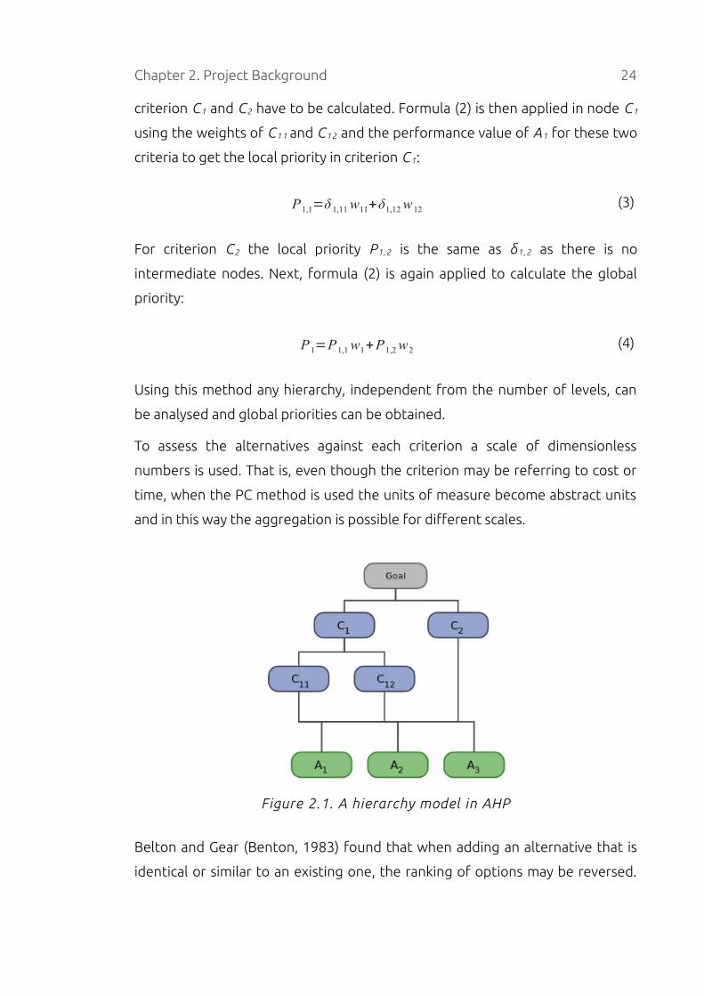
Chapter 2. Project Background 24
criterion C1 and C2 have to be calculated. Formula (2) is then applied in node C1
using the weights of C11 and C12 and the performance value of A1 for these two
criteria to get the local priority in criterion C1:
P1,1=δ 1,11 w11+δ1,12 w12 (3)
For criterion C2 the local priority P1,2 is the same as δ1,2 as there is no
intermediate nodes. Next, formula (2) is again applied to calculate the global
priority:
P1=P1,1 w1+P1,2 w2 (4)
Using this method any hierarchy, independent from the number of levels, can
be analysed and global priorities can be obtained.
To assess the alternatives against each criterion a scale of dimensionless
numbers is used. That is, even though the criterion may be referring to cost or
time, when the PC method is used the units of measure become abstract units
and in this way the aggregation is possible for different scales.
Figure 2.1. A hierarchy model in AHP
Belton and Gear (Benton, 1983) found that when adding an alternative that is
identical or similar to an existing one, the ranking of options may be reversed.
Chapter 2. Project Background 25
To prevent this, they developed the Ideal Mode AHP . In this mode, instead of
having the performance values of the alternatives for a given criterion sum to 1,
each value is divided by the maximum value in the vector so the resulting vector
has a maximum value of 1 instead of the sum being 1.
2.3 Pairwise Comparison (PC) Method
To assess the alternatives under a given criterion, it is often very hard for DMs
to assign an absolute score. Qualitative and quantitative data may be
unavailable or necessary information to quantify the performance of
alternatives may be incomplete. Therefore, the PC method is used to determine
the relative importance or weights of the alternatives and criteria with respect
to each criterion in the decision problem.
Under this approach, the DM has to analyse only two elements at a time. To
make this comparison, the DM has to choose a value indicating how many times
more important, preferred or dominant one element is over another element in
terms of a given criterion. This value has to be given in reference to a
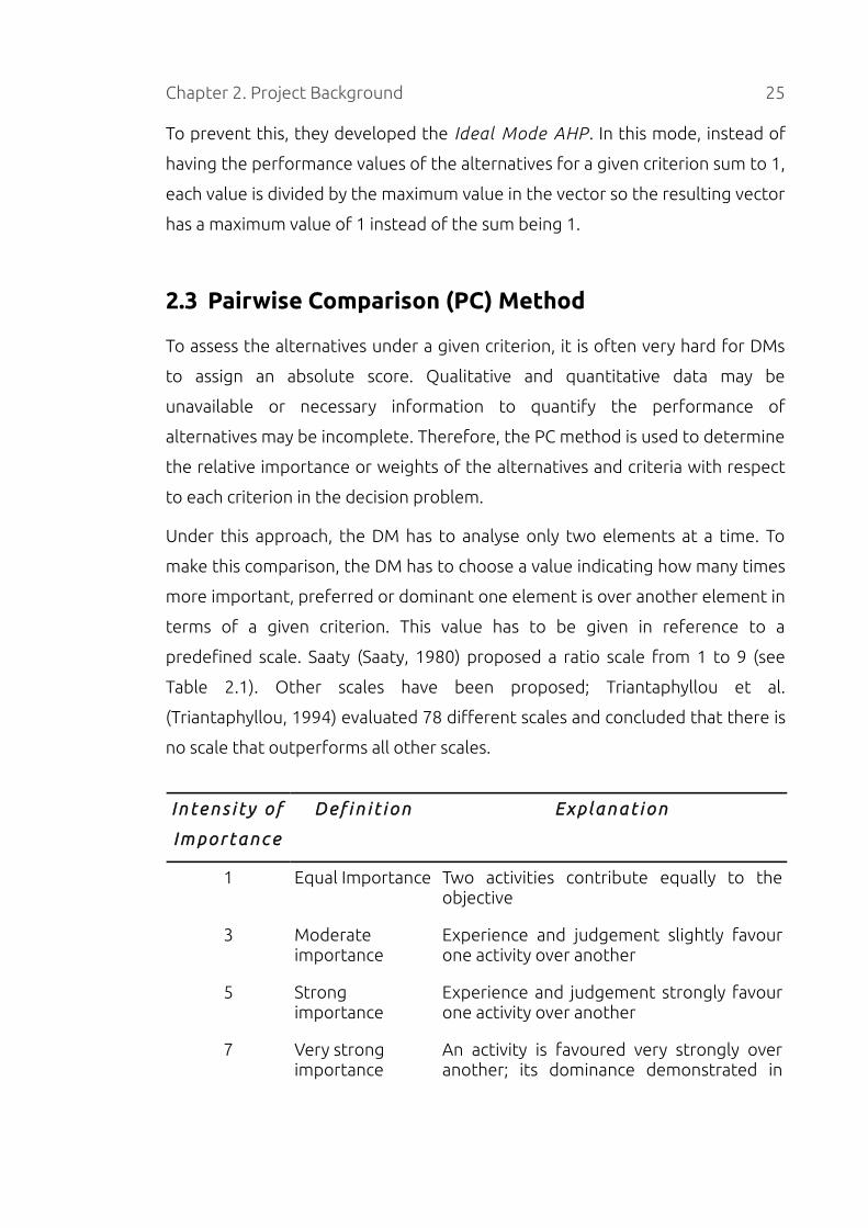
predefined scale. Saaty (Saaty, 1980) proposed a ratio scale from 1 to 9 (see
Table 2.1). Other scales have been proposed; Triantaphyllou et al.
(Triantaphyllou, 1994) evaluated 78 different scales and concluded that there is
no scale that outperforms all other scales.
I n t e n s i t y o f
I m p o r t a n c e
D e f i n i t i o n E x p l a n a t i o n
1 Equal Importance Two activities contribute equally to the objective
3 Moderate importance
Experience and judgement slightly favour one activity over another
5 Strong importance
Experience and judgement strongly favour one activity over another
7 Very strong importance
An activity is favoured very strongly over another; its dominance demonstrated in

Chapter 2. Project Background 26
I n t e n s i t y o f
I m p o r t a n c e
D e f i n i t i o n E x p l a n a t i o n
practice
9 Extreme importance
The evidence favouring one activity over another is of the highest possible order of affirmation
2,4,6,8 Intermediate values
1.1-1.9 If the activities are very close
May be difficult to assign the best value but when compared with other contrasting activities the size of the small numbers would not be too noticeable, yet they can still indicate the relative importance of the activities
Table 2.1. Scale of Relative Importance (Saaty, 1980)
When comparing elements A i and A j, A i is said to be a i j times more important
than A j, and the reciprocal value of the judgement is used to score the inverse
comparison, that is, A j is a j i times more important than A i. The self-comparison
a i i is always scored 1 (See formula 5).
a ij=1a ji
, aii=1 (5)
All judgements of the elements with respect to a given criterion are organised
in a PC matrix (PCM). For n elements, the matrix is of size n x n, and because of
the constraints in formula (5), only n(n-1)/2 elements are provided by the DM.
A=[1 a12 a13 ⋯ a1n
1/a12 1 1/ a23 ⋯ a2n
1/a13 1/a23 1 ⋯ a3n⋯ ⋯ ⋯ ⋯ ⋯
1/a1n 1/a2n 1/a3n ⋯ 1] (6)
There exists the possibility that the DM may provide inconsistent judgements.

Chapter 2. Project Background 27
For instance, if a12=3, a23=2, then we would expect that a13=6. However, this is
rarely the case. A PC matrix is said to be consistent or acceptable if its
corresponding Consistency Ratio (CR3) is less than 0.1 (Saaty, 1980). There exist
two types of consistency (Siraj, 2011), cardinal consistency (CC) and ordinal
consistency (OC). For a matrix to be cardinally consistent, the condition
a i j=a ikakj must hold true for all i, j, k. The ordinal consistency refers to the
transitivity of the preferences, if alternative A i is preferred over A j, and A j is
preferred over Ak, then A i should be preferred over Ak. When this is condition is
not met, the matrix is said to be ordinally inconsistent and it is not possible to
find a weight vector that satisfies all preferences directions.
If the alternative A i is preferred over A j but the derived priorities are such that
wj > wi, then a priority violation is present (Mikhailov, 1999). If the matrix is
ordinally inconsistent, then priority violations may occur.
2.4 Elicitation Methods
To derive the weights or priorities from the PC matrix different methods may
be used. For consistent matrices, generally all methods yield similar results only
differing in intensities. Siraj (Siraj, 2011) analysed several methods and
proposed two new methods based on graph theory and multi-objective
optimisation: Enumerating All Spanning Trees (EAST) and Prioritisation using
Indirect Judgements (PrInT). PrInT outperformed all other methods for
inconsistent matrices. Based on their simplicity, however, the most common
methods used to elicit priorities in AHP are Eigenvector (EV), Geometric Mean
(GM) and Normalised Column Sum (NCS).
Some other methods are: Column-Row Orientation (Comrey, 1950), Direct Least
Squares (DLS) (Chu, 1979), Weighted Least Squares (WLS) (Chu, 1979),
Logarithmic Least Absolute Value (LLAV) (Cook, 1988), Logarithmic Least
Squares (LLS) (Crawford, 1987), Fuzzy Preference Programming (FPP)
(Mikhailov, 2000) and Two-Objective Prioritisation (TOP) (Mikhailov, 2006).
A study by Choo and Wedley (Choo, 2004) evaluated 18 different methods and
3 Also known as the Consistency Index (CI)
Chapter 2. Project Background 28
recommended GM and NCS for their easy calculation and good performance on
consistent and inconsistent matrices.
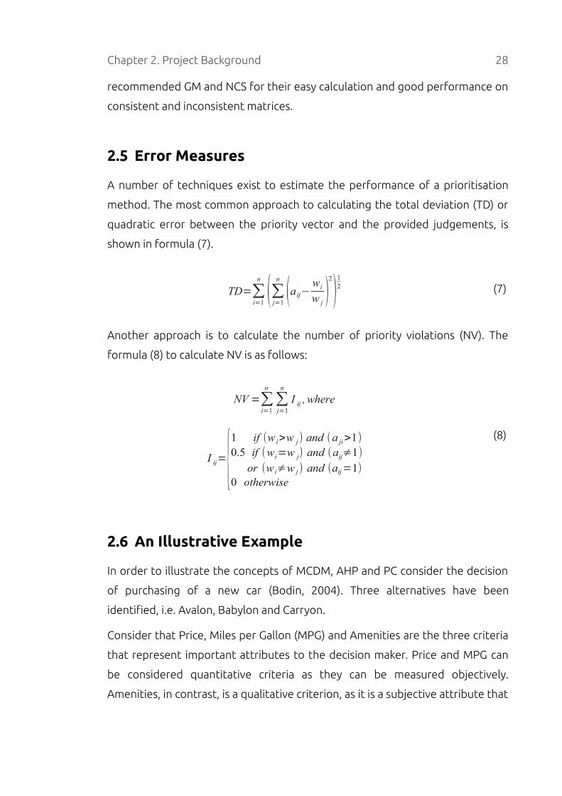
2.5 Error Measures
A number of techniques exist to estimate the performance of a prioritisation
method. The most common approach to calculating the total deviation (TD) or
quadratic error between the priority vector and the provided judgements, is
shown in formula (7).
TD=∑i=1
n
(∑j=1
n
(a ij−wi
w j)
2
)12
(7)
Another approach is to calculate the number of priority violations (NV). The
formula (8) to calculate NV is as follows:
NV =∑i=1
n
∑j=1
n
I ij , where
I ij={1 if (w i>w j) and (a ji>1)
0.5 if (wi=w j) and (aij≠1)
or (w i≠w j) and (aij=1)0 otherwise
(8)
2.6 An Illustrative Example
In order to illustrate the concepts of MCDM, AHP and PC consider the decision
of purchasing of a new car (Bodin, 2004). Three alternatives have been
identified, i.e. Avalon, Babylon and Carryon.
Consider that Price, Miles per Gallon (MPG) and Amenities are the three criteria
that represent important attributes to the decision maker. Price and MPG can
be considered quantitative criteria as they can be measured objectively.
Amenities, in contrast, is a qualitative criterion, as it is a subjective attribute that

Chapter 2. Project Background 29
depends on the point of view of the DM. Furthermore, the DM identifies
Prestige, Comfort and Style as Amenities' sub-criteria. The hierarchy tree
representing this decision problem is shown in Figure 2.2.
Figure 2.2. Car selection example
In order to make a decision, the DM has to give pairwise comparison
judgements at every level of the hierarchy. In general terms, the attributes
Price, Comfort and Prestige are of major importance to the DM, while he/she is
less concerned about MPG and Style.
The DM gives the following judgements for the first level.
– Price has a strong or very strong importance when compared to MPG
– Price has a moderate importance when compared to Amenities
– Amenities has a moderate or strong importance when compared to
MPG.
Table 2.1 is used in order to convert these verbal judgements into numeric
values. As a consequence, Price is 6 times as important as MPG, Price is 3 times
as important as Amenities and Amenities is 4 times as important as MPG, as
represented in Table 2.2. The inverse comparison is evaluated with the
Chapter 2. Project Background 30
reciprocal value and the self-comparison is evaluated with 1.
Price MPG Amenities
Price 1 6 3
MPG 1/6 1 1/4
Amenities 1/3 4 1
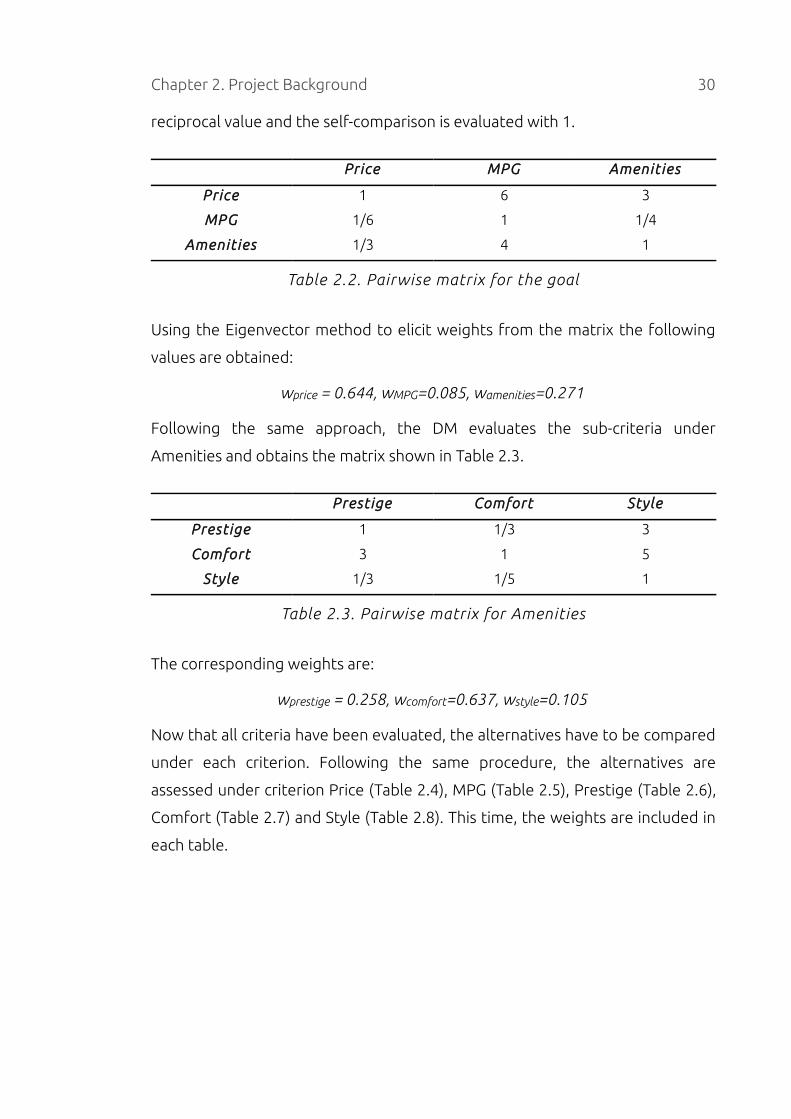
Table 2.2. Pairwise matrix for the goal
Using the Eigenvector method to elicit weights from the matrix the following
values are obtained:
wprice = 0.644, wMPG=0.085, wamenities=0.271
Following the same approach, the DM evaluates the sub-criteria under
Amenities and obtains the matrix shown in Table 2.3.
Prestige Comfort Style
Prestige 1 1/3 3
Comfort 3 1 5
Style 1/3 1/5 1
Table 2.3. Pairwise matrix for Amenities
The corresponding weights are:
wprestige = 0.258, wcomfort=0.637, wstyle=0.105
Now that all criteria have been evaluated, the alternatives have to be compared
under each criterion. Following the same procedure, the alternatives are
assessed under criterion Price (Table 2.4), MPG (Table 2.5), Prestige (Table 2.6),
Comfort (Table 2.7) and Style (Table 2.8). This time, the weights are included in
each table.
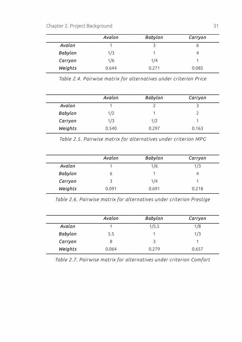
Chapter 2. Project Background 31
Avalon Babylon Carryon
Avalon 1 3 6
Babylon 1/3 1 4
Carryon 1/6 1/4 1
Weights 0.644 0.271 0.085
Table 2.4. Pairwise matrix for alternatives under criterion Price
Avalon Babylon Carryon
Avalon 1 2 3
Babylon 1/2 1 2
Carryon 1/3 1/2 1
Weights 0.540 0.297 0.163
Table 2.5. Pairwise matrix for alternatives under criterion MPG
Avalon Babylon Carryon
Avalon 1 1/6 1/3
Babylon 6 1 4
Carryon 3 1/4 1
Weights 0.091 0.691 0.218
Table 2.6. Pairwise matrix for alternatives under criterion Prestige
Avalon Babylon Carryon
Avalon 1 1/5.5 1/8
Babylon 5.5 1 1/3
Carryon 8 3 1
Weights 0.064 0.279 0.657
Table 2.7. Pairwise matrix for alternatives under criterion Comfort

Chapter 2. Project Background 32
Avalon Babylon Carryon
Avalon 1 1/7 1/4
Babylon 7 1 3.5
Carryon 4 1/3.5 1
Weights 0.077 0.679 0.244
Table 2.8. Pairwise matrix for alternatives under criterion Style
To calculate the global ranking of the alternatives formula (2) is applied to each
node of the hierarchy to obtain the local contribution, and then the results are
aggregated. For example, to obtain the local contribution of alternative Avalon
to the node Amenities is as follows:
Pavalon,amenities = δavalon,prestige * wprestige + δavalon,comfort * wcomfort + δavalon,style
* wstyle
= 0.091 * 0.258 + 0.064 * 0.637 + 0.077 * 0.105
= 0.0723
And the global priority is calculated as:
Pavalon = δavalon,price * wprice + δavalon,MPG * wMPG + δavalon,amenities * wamenities
= 0.644 * 0.644 + 0.540 * 0.085 + 0.0723 * 0.271
= 0.48
The priority for Babylon and Carryon are calculated in a similar way, resulting in
the final ranking of alternatives as:
Pavalon = 0.48, Pbabylon = 0.32, Pcarryon = 0.20
The highest rated car is Avalon with 48%, followed by Babylon with 32% and
Carryon with 20%. As a consequence, the outcome suggest that the DM should
purchase the Avalon car.
Consider if the price of Babylon is reduced by a 20%, would Avalon be still the
highest rated car? Similarly, how much would the price of Babylon have to be
reduced, or the price of Avalon increased, to change the suggested
recommendation? Or for example, if the DM is not completely sure about the

Chapter 2. Project Background 33
judgements between Style and Prestige, how would that affect the solution?
These kind of questions can be answered by conducting a sensitivity analysis
(SA) on the results.
2.7 Sensitivity Analysis
The solution to a decision problem, the global ranking of alternatives, may not
provide enough information to the DM to make a final decision. There are
several reasons why a sensitivity analysis (SA) should be conducted on the
results. For instance, the judgements for some criteria may be subjective or
there may be uncertainty in the data that leads to the preference value. In
addition, the preference judgements may come from a group decision where
there are different opinions. Moreover, different prioritisation methods may
yield different results for the same PC matrix; at the same time different
performance scoring scales used in evaluating alternatives may produce
different rankings (Steele, 2009). An SA provides more insight about the
problem and in this way the DM should be able to make a more informed
decision.
Methods to perform SA on AHP problems may be grouped into three main
categories (Chen, 2008): numerical incremental analysis, probabilistic
simulations and mathematical models.
2.7.1 Numerical Incremental Analysis
This approach involves changing the weight values and calculating the new
solution. The method, also known as One-at-a-time (OAT), works by
incrementally changing one parameter at a time, calculating the new solution
and graphically presenting how the global ranking of alternatives changes. This
is the most commonly used method in associated software tools ((SIMUL8,
2012), (MakeItRational, 2012), (ExpertChoice, 2012), (SAL, 2012), (IDS, 2010))
and, according to Chen and Kocaoglou (Chen, 2008), is also the most popular in
the literature where AHP is used to solve problems.
Chapter 2. Project Background 34
As AHP uses WSM to aggregate local priorities, the global weights are a linear
function depending on the local contributions. Given this property, the global
priorities of alternatives can be expressed as a linear function of the local
weights. Furthermore, if only one weight w i is changed at a time, the priority P i
of alternative A i can be expressed as a function of w i using the following
formula:
P i=P i
' '−P i
'
w i' '−wi
' (w i−wi')+ P i ' (9)
where P i' ' and P i
' are the priority values for w i' ' and w i
' respectively. With this
method, only two iterations are necessary to produce a chart with the values of
priorities of all alternatives for the range 0 to 1 of one of the weights, as shown
in Figure 2.3.
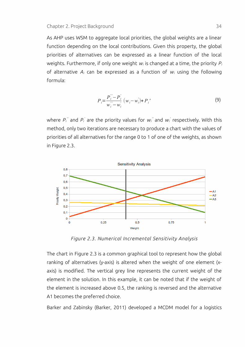
Figure 2.3. Numerical Incremental Sensitivity Analysis
The chart in Figure 2.3 is a common graphical tool to represent how the global
ranking of alternatives (y-axis) is altered when the weight of one element (x-
axis) is modified. The vertical grey line represents the current weight of the
element in the solution. In this example, it can be noted that if the weight of
the element is increased above 0.5, the ranking is reversed and the alternative
A1 becomes the preferred choice.
Barker and Zabinsky (Barker, 2011) developed a MCDM model for a logistics
Chapter 2. Project Background 35
problem and proposed a method for finding the weights where a rank reversal4
is produced in the model. The approach they used can be generalised to other
problems. As only one weight wk is changed at a time, all other weights w l can
be expressed as a function of wk. Then, formula (2) can be expressed as a
function of only one variable weight wk. By solving the equation P i=P j, the value
wk where the ranking of both alternatives is the same (rank reversal) can be
found.
Another approach proposed by Hurley (Hurley, 2001) multiplies the preference
judgements in the PC matrix by a constant value and then the solution is
recalculated using this new matrix. For constant values greater than 1, weights
diverge; for values lower than 1, weights converge. Although this method will
not produce a rank reversal, Hurley states that it may be useful to test the
magnitude of the numerical weights elicited from the matrix.
2.7.2 Probabilistic Simulations
Simulation methods replace judgements in the PC matrix with values from
probability distributions and perform a number of simulations to calculate the
expected ranking of alternatives. As probabilistic input is used, the problem is
no longer deterministic. In contrast with the previous method, this approach
allows for changing more than one parameter at a time.
Butler et al. (Butler, 1997) proposed a method using Monte-Carlo simulations
that allows random change of all weights simultaneously to explore the effect
on the ranking. They presented three types of simulations:
1. Random weights
All criteria weights are generated completely at random in order to discover
how the ranking of the alternatives changes under any conditions. To generate
n weights, n-1 random numbers are generated in the interval 0-1 using a
uniform random number generator. These numbers are sorted so that 1 > rn-1
> rn-2 > … > r2 > r1 > 0. In addition, let rn=1 and r0=0. The value for the weight
w' i is calculated as w' i = r i – r i -1, for i=1..n. The vector W'=[w'1,...,w'n] will sum
4 Rank reversal occurs in line intersections in Figure 2.3
Chapter 2. Project Background 36
to 1 and is uniformly distributed.
By performing many repetitions of these steps a great number of times (5.000
iterations are used in the example), the entire domain of possible weight
combinations can be explored.
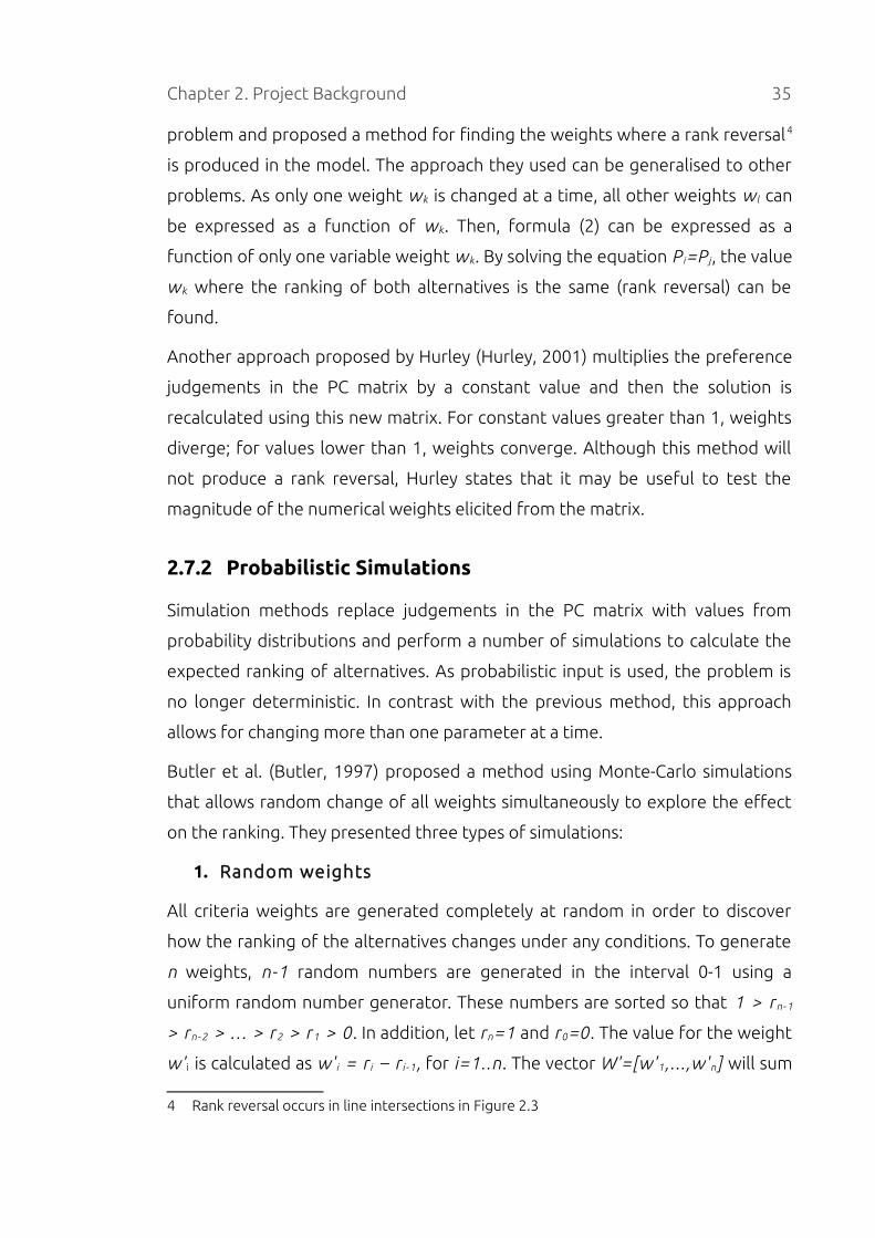
For every iteration, the solution is calculated with random weights and the
ranking of the alternatives is registered. After the simulation is finished, a
statistical analysis can be performed to find information about the distribution
of the ranking of alternatives. For instance, a box-plot chart may be created (see
Figure 2.4) to depict information about the ranking of alternatives.
Figure 2.4. Box-plot Chart Presenting Simulation Results
The black diamonds correspond to the mean ranking, the blue box encloses quartiles
Q1-Q3 (25%-75% of the samples had this ranking), and the minimum and maximum
ranks are the endpoints of the grey lines (Butler, 1997).
Chapter 2. Project Background 37
2. Random weights preserving rank order
If the ranking of criteria weights are of importance and have to be preserved,
then the procedure is similar to the previous one with the difference that the
random weights are ranked according to the original criteria ranking and then
are used to calculate the solution. The chart presented in Figure 2.4 is still valid
when using this method.
3. Random weights from a response distribution
This type of simulation considers the current weights as means of probability
distributions and the random weights for the simulation are generated from
these distributions. Even though the random weights may be relatively close to
the real weights, this approach may generate weights with a different rank
order than the actual weights.
The formula to generate the random weights is:
w i'=
X i
X i+...+ X n
,where X i∼Gamma(w i ,β) (10)
The variation from the mean of the generated values can be controlled with the
β parameter. Again, the procedure is similar, changing only the way random
weights are generated.
A similar simulation approach, introduced by Hauser and Tadikamalla (Hauser,
1996), explores the effects of changing the judgements in the PC matrices. The
method varies the preference values from the pairwise comparisons by creating
an interval for each element of the matrix. The midpoint of the interval is the
current value of the judgement and the width of the interval is defined by a
constant c indicating the distance from the central point as a percentage. If a i j is
the preference value, then the interval I i j may be represented as I i j = [a i j – c a i j,
a i j + c a i j]. The next step is to generate random numbers for each interval for
each of the matrices in the model. Any probability distribution may be used.
Hauser and Tadikamalla used the uniform distribution and the triangular
distribution to test the method. Then, the random numbers have to be
converted to the AHP scale using the formula (11):
Chapter 2. Project Background 38
a ij'={
12−r
if r <1
r if r⩾1 (11)
For every iteration, the solution is calculated with the random judgements and
the ranking of the alternatives is registered. As with Butler's method (Butler,
1997), a statistical analysis can be performed to find information about the
distribution of the ranking of alternatives.
In addition, Hauser and Tadikamalla proposed a formula to express the final
ranking of the alternatives as statistical weights representing the expected
weights for the given probability distribution, according to formula (12).
ES i=∑k=1
n
pik (n+1−k ) , for i=1...n
EW i=ES i
∑k =1
n
ES k
, for i=1...n (12)
2.7.3 Mathematical Models
This group of SA methods uses mathematical models when it is possible to
express the relationship between the input data and the problem solution.
Mathematical models have better performance and are more efficient than the
previous methods as they do not require iteration. Moreover, their results are
much more accurate when using verified formulas.
Several authors have developed mathematical models for SA in AHP. Masuda
(Masuda, 1990) studied how changes throughout the whole domain in the
weights of criteria may affect the ranking of alternatives and proposed a
sensitivity coefficient representing the possibility of rank reversal from these
changes. Huang (Huang, 2002) found an inconsistency in Masuda's coefficient
as a large value of the coefficient may not necessarily mean that a rank reversal
will occur, and vice versa, a low value of the coefficient may produce a rank
reversal. To overcome this, Huang proposed a new sensitivity coefficient and
Chapter 2. Project Background 39
demonstrated it reveals the sensitivity of an AHP model with more accuracy
than Masuda's coefficient.
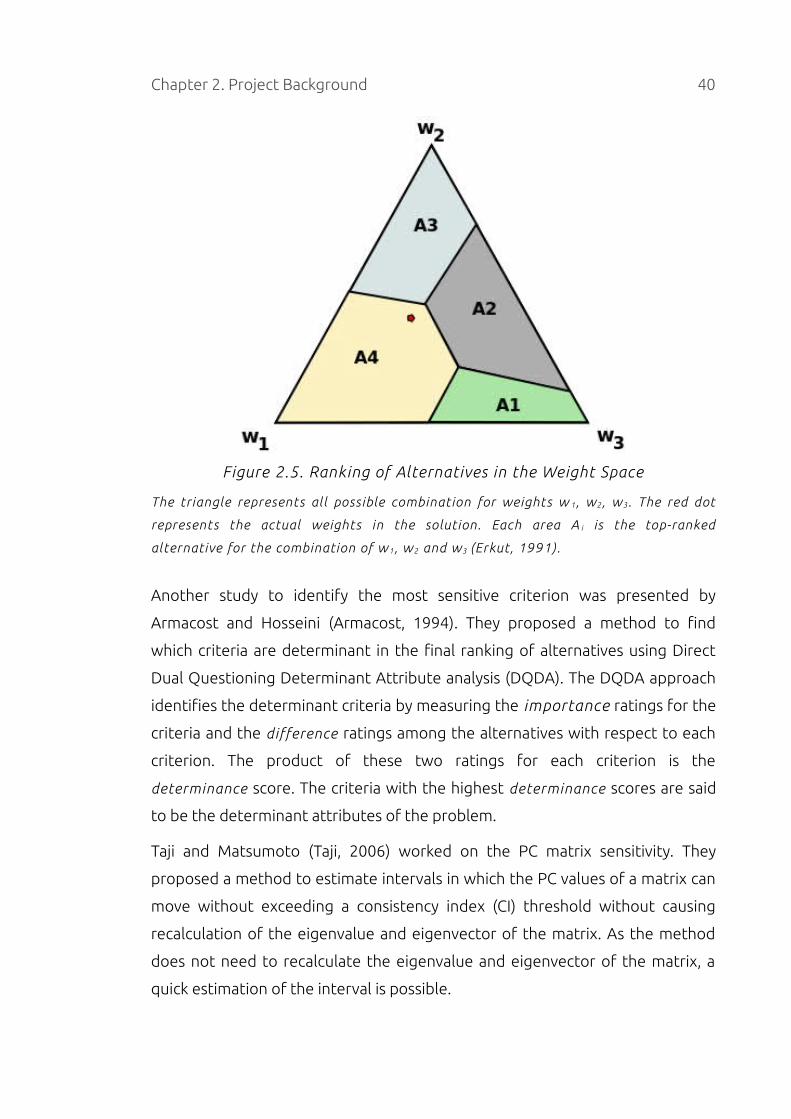
Erkut and Tarimcilar (Erkut, 1991) presented a method to analyse and visualise
in the weight space (see Figure 2.5) the ranking of alternatives with respect to
all possible combinations of weights for the first level of criteria. The method
works by partitioning the weight space T into n subsets S i, where n is the
number of criteria. The weight space refers to all possible combinations of
weights, as shown in formula (13):
(w1, w2, ... , wn) , where 0≤wi≤1 ∧ ∑i=1
n
wi=1 (13)
For three criteria the weight space is a triangle-shaped plane with corners in
(1,0,0), (0,1,0) and (0,0,1). For n=3 criteria and m alternatives, Erkut and
Tarimcilar provide a method for partitioning T into m subsets where in each
subset some alternative has the highest ranking. The relative areas of these
subsets indicate which alternatives are more likely to be selected.
However, there are limitations in their method. It does not provide a method
for performing sensitivity analysis when the problem has more than one level of
criteria. In addition, if more than three criteria are simultaneously considered,
then visual representation is not possible and the weight space T is no longer a
triangle, it becomes a convex polyhedron. Moreover, two extra algorithms have
to be used to perform the partitioning (Balinski, 1961) and the calculation of
the volumes (Cohen, 1979) (instead of areas) of the subsets.
Trantaphyllou and Sánchez (Triantaphyllou, 1997) investigated the sensitivity
analysis for problems with one level of criteria by examining the impact of
changes in the weights of criteria and changes in the weights of alternatives
with respect to a single criterion at a time. They proposed a method to identify
the most critical criterion (for criteria weights and for alternative weights) and
the quantity by which it needs to be modified so that the top-ranked alternative
will change. In addition, they introduced a sensitivity coefficient as an indicator
of how sensitive to changes are the elements in the decision problem.
Chapter 2. Project Background 40
Figure 2.5. Ranking of Alternatives in the Weight Space
The triangle represents all possible combination for weights w 1 , w2 , w3. The red dot
represents the actual weights in the solution. Each area A i is the top-ranked
alternative for the combination of w 1 , w2 and w3 (Erkut, 1991).
Another study to identify the most sensitive criterion was presented by
Armacost and Hosseini (Armacost, 1994). They proposed a method to find
which criteria are determinant in the final ranking of alternatives using Direct
Dual Questioning Determinant Attribute analysis (DQDA). The DQDA approach
identifies the determinant criteria by measuring the importance ratings for the
criteria and the difference ratings among the alternatives with respect to each
criterion. The product of these two ratings for each criterion is the
determinance score. The criteria with the highest determinance scores are said
to be the determinant attributes of the problem.
Taji and Matsumoto (Taji, 2006) worked on the PC matrix sensitivity. They
proposed a method to estimate intervals in which the PC values of a matrix can
move without exceeding a consistency index (CI) threshold without causing
recalculation of the eigenvalue and eigenvector of the matrix. As the method
does not need to recalculate the eigenvalue and eigenvector of the matrix, a
quick estimation of the interval is possible.
Chapter 2. Project Background 41
Chen and Kocaoglu (Chen, 2008) proposed an algorithm to examine the impact
of single or multiple changes to the weights of criteria or alternatives at any
level of the AHP hierarchy. Their approach finds the allowable range of changes
in order to prevent a rank reversal. In addition, two sensitivity coefficients are
presented and the most critical criterion in each level of the hierarchy is
identified.
Iryanto (Iryanto, 2006) investigated the sensitivity of Interval AHP (IAHP). In
IAHP, judgements in the PC matrix are provided as intervals instead of single
values. Weights are elicited from the PC matrix using linear programming by
minimising the error between the weight vector and the geometric mean of
each interval. Iryanto concluded that when changes are introduced to an
interval, as long as the limits of the new interval remain inside the original
interval, the ranking is preserved.
Chen and Li (Chen, 2011) have recently developed a method to conduct SA
using the column-row orientation elicitation method (Comrey, 1950). This
algorithm calculates the allowable range of judgement perturbations induced
in a PC matrix at any level of the decision hierarchy in order to keep the current
ranking of alternatives unchanged.
2.8 Summary
This chapter has presented an overview of MCDM, AHP and PC. In addition, a
discussion of SA was presented and its different types were covered.
Sensitivity analysis methods may be grouped into three main categories:
numerical incremental analysis, probabilistic simulations and mathematical
models. The first method is the most popular because of its simplicity and easy
implementation. However, the other two groups of methods may provide more
insights on a decision problem as they allow simultaneous analysis on more
than one decision element.

Chapter 3
Requirements for AHP Software
This chapter focuses on common criteria for evaluating AHP tools. The focus is
on features for the AHP and PC techniques described in the previous chapter.
The aim is to create a framework to analyse available software tools and
examine to what extent they comply with these features.
3.1 Requirements for Evaluating Software
There is limited literature on this subject. A number of studies ((Buede, 1992),
(Buede, 1996), (Weistroffer, 1997)) have reviewed MCDM software in terms of
general attributes such as platform, price and methodology5. Other study
(Ossadnik, 1999) evaluated AHP software based on the model ISO/IEC 9126
(Caia, 2011). However, no study appears to have focused on evaluating AHP
features and SA.
From the material presented in Chapter 2, the main features expected in an
AHP software tool are described below (Sections 3.1.1 and 3.1.2). They are
divided into two groups: support for AHP and PC, and support for SA.
3.1.1 Support for AHP and PC
AHP software should support hierarchical models, pairwise comparison,
numeric and verbal scales, consistency analysis, methods for elicitation and
provide performance measures.
A1. Hierarchical models: a tool should allow a hierarchy model with
arbitrary levels of criteria and number of alternatives. In this way, any decision
problem can be modelled as a hierarchy and solved using AHP.
A2. PC for criteria and alternatives: pairwise comparison should be
available to provide judgements for criteria and for alternatives with respect to
5 Methodology refers to the alternative ranking method used, e.g. AHP (Saaty, 1980), MAUT
(Wallenius, 2008), ELECTRE (Roy, 1968).
42

Chapter 3. Requirements for AHP Software 43
a criterion. This means that at every level of the hierarchy the weights of the
elements should be elicited from pairwise comparisons.
A3. Numerical and verbal scales: the scale to provide the judgements
should be both numerical and verbal, as shown in Table 2.1.
A4. Consistency analyser: to assist the DM to improve consistency of the
PC matrix, its consistency index (CI), ordinal consistency and cardinal
consistency should be displayed.
A5. Prioritisation methods: a software tool should support more than
one prioritisation method so DMs can evaluate different methods and choose a
solution according to their needs.
A6. Error measures: Error measures (TD, NV) must be provided so the DM
can get an indicator of the deviation of the solution from the provided
judgements.
3.1.2 Support for Sensitivity Analysis
As discussed in Section 2.7, there are several approaches to conduct an SA in
AHP. We conclude that an AHP tool should provide each of the three forms of
SA identified: numerical incremental analysis, probabilistic simulation and
mathematical models. In addition, the most sensitive criteria should be
presented.
B1. Numerical incremental analysis: a module for performing the one-
at-a-time sensitivity analysis should be provided, along with a graph similar to
the one presented in Figure 2.3 to display the sensitivity of a criterion.
B2. Probabil istic simulation: a module for performing probabilistic
simulations should be provided in order to find the sensitivity of alternatives to
simultaneous changes in all weights, including a graph similar to the one
depicted in Figure 2.4.
B3. Mathematical models: using the mathematical approach to SA the
threshold values for the weights that produce a rank reversal should be
presented in a graph similar to the one shown in Figure 2.5.
Chapter 3. Requirements for AHP Software 44
B4. Most sensitive criteria: along with the results of the SA, the most
sensitive criteria should be presented and sensitivity coefficients should be
included so the DM can have an estimation of how sensitive is each criterion.
B5. Number of simultaneous changes: the number of elements that
can be changed at the same time to analyse the results; more than one
simultaneous change should be supported.
3.2 Software Products
In this section, four commercial or research prototype tools that support AHP
and PC are analysed in terms of the framework described above: Expert Choice
(ExpertChoice, 2012), MakeItRational (MakeItRational, 2012), PriEsT (Siraj,
2012a) and Web-HIPRE (SAL, 2012).
For each feature (A1-A5, B1-B5) a score between 0 and 3 will be assigned: 0 if
the feature is not present, 1 if it is poorly implemented, 2 if it is moderately
supported, and 3 if it is fully supported. The overall score for a tool will be the
sum of the individual scores.
3.2.1 Expert Choice
Expert Choice ((ExpertChoice, 2012), (Ishizaka, 2009), (Chan, 2007)) is a
commercial desktop-based application for Windows that enables DMs to
prioritise and evaluate criteria and alternatives using AHP. The analysis is
detailed in Table 3.1. It is worth noting that Expert Choice only supports the
basic form of SA, i.e. changing one parameter at a time and presenting the
results. Its overall score is 13 out of 33.
F e a t u r e S c o r e D e s c r i p t i o n
A1 3
Expert Choice provides a GUI to build an arbitrary-depth
hierarchy (student version is limited to 3 levels). Elements
can be added, edited and removed from the model
A2 3 The software supports pairwise comparison in all levels of

Chapter 3. Requirements for AHP Software 45
F e a t u r e S c o r e D e s c r i p t i o n
the hierarchy
A3 3The judgements may be entered using a numeric or verbal
scale
A4 1Only the consistency index is displayed. No information
about cardinal or ordinal inconsistency is presented
A5 0Only the eigenvector method is included in the software.
There is no option to change the method or add new ones
A6 0No error measures are presented when calculating the
weight vector
B1 2
Numerical incremental analysis is supported with three
graphs that allows to change the weights of one criterion.
It is not possible to change the weights of alternatives
with respect to one criterion, only criteria weights
B2 0 Expert Choice does not support probabilistic simulations
B3 0
There is no support for identifying the threshold values
for rank reversal. It has to be done manually using the
numerical incremental analysis
B4 0No sensitivity coefficient is provided and the most
sensitive elements are not identified
B5 1 Only one parameter can be modified at a time
Table 3.1. Expert Choice Software Evaluation
3.2.2 MakeItRational
MakeItRational (MakeItRational, 2012) is a commercial web-based application
for decision making with a user-friendly interface. It requires the Silverlight
plugin from Microsoft to run on a supported web-browser. The analysis is
detailed in Table 3.2. Its overall score is 12 out of 33.

Chapter 3. Requirements for AHP Software 46
F e a t u r e S c o r e D e s c r i p t i o n
A1 3
MakeItRational provides a GUI to build an arbitrary-depth
hierarchy. Elements can be added, edited and removed
from the model
A2 3Pairwise comparisons – or direct rating- are supported in all
levels of the hierarchy
A3 2Judgements are entered using a numerical scale, however,
a description is available for each number of the scale
A4 3
The software includes the consistency index and hints for
helping the DM to improve the ordinal and cardinal
consistency when the judgements are inconsistent
A5 0Only the eigenvector method is included in the software.
There is no option to change the method or add new ones
A6 0No error measures are presented when calculating the
weight vector
B1 1
Numerical incremental analysis is supported with one
static graph similar to the one in Figure 2.3. It does not
allow to change the weights of criteria or alternatives
B2 0 No support for probabilistic simulations
B3 0
There is no support for identifying the threshold values for
rank reversal. It has to be done manually using the graph
from the numerical incremental analysis
B4 0No sensitivity coefficients are provided and the most
sensitive elements are not identified
B5 0 No changes are possible. The sensitivity graph is static
Table 3.2. MakeItRational Software Evaluation
3.2.3 PriEsT
PriEsT is an open source tool developed at the University of Manchester (Siraj,

Chapter 3. Requirements for AHP Software 47
2012a) that provides decision support based on AHP and PC. PriEsT is
implemented in Java and is currently available for Linux and Windows. The
overall score for this tool is 16 out of 33. The results from the analysis are
presented in Table 3.3.
F e a t u r e S c o r e D e s c r i p t i o n
A1 2
PriEsT supports an unlimited number of decision elements
and levels in the hierarchy. Elements can be added and
edited, but not removed from the model
A2 3Pairwise comparisons are supported in all levels of the
hierarchy
A3 2Judgements can be entered using only a numerical scale - a
verbal scale is not supported
A4 3
The consistency index, cardinal and ordinal consistency
measures are displayed as well as hints for helping the DM
to improve overall consistency of the judgements
A5 3PriEsT supports 11 prioritisation methods which can be
selected to derive weights
A6 3Error measures TD, NV and TD2 (total deviation using
indirect judgements (Siraj, 2011)) are presented
B1-B5 0 PriEsT has no support for sensitivity analysis
Table 3.3. PriEsT Software Evaluation
3.2.4 Web-HIPRE
Web-HIPRE (SAL, 2012) is a free web-based application for MCDM implemented
as a Java applet. It was the first decision tool available online (Mustajoki, 2000).
Table 3.4 presents the analysis of the software according to the previously
defined features. The overall score is 14 out of 33.

Chapter 3. Requirements for AHP Software 48
F e a t u r e S c o r e D e s c r i p t i o n
A1 3
Hierarchies of up to 17 levels can be defined using the web
interface – this is enough for most problems. Elements can
be added, edited and removed from the model
A2 3Pairwise comparisons are supported in all levels of the
hierarchy
A3 3Judgements can be entered using a numerical or verbal
scale
A4 1
Only the consistency index is displayed. No information
about cardinal or ordinal inconsistency is presented. No
hints for improving the consistency of the judgements
A5 0
Only the eigenvector method is included in the software
when working with AHP. There is no option to change the
method or add new ones
A6 0No error measures are presented when calculating the
weight vector
B1 3
Numerical incremental analysis is supported with a
dynamic graph similar to the one in Figure 2.3. It allows to
change the weights of one element (criterion or
alternative)
B2 0 No support for probabilistic simulations
B3 0
There is no support to identify threshold values for rank
reversal. This has to be done manually for each criterion
using the graph from the numerical incremental analysis
B4 0No sensitivity coefficients are provided and the most
sensitive elements are not identified
B5 1 Only one parameter can be modified at a time
Table 3.4. Web-HIPRE Software Evaluation

Chapter 3. Requirements for AHP Software 49
Out of a maximum possible score of 33, PriEsT Is ranked first with a score of 16
followed by Web-HIPRE with 14. The analysis shows that all tools have similar
support for AHP and PC, the most significant difference is that only PriEsT
provides more than one elicitation method and presents error measures with
the results. PriEsT is the only tool with no support for SA; other tools provide a
basic form of SA using the numerical incremental analysis. No tool provides
sensitivity coefficients or identification of the most sensitive criteria. The lack of
these features contributed to the relative low score of all the software tools.
As PriEsT has obtained the highest overall score, it has been selected to be
enhanced by including a module for conducting the three types of SA - features
B1-B5 - and features A1 and A3, as it scored 2 out of 3 for these two criteria. A
brief introduction to PriEsT is given next.
3.3 An Overview of PriEsT
PriEsT (Priority Estimation Tool) is a decision support tool for AHP and PC that
helps DMs to identify inconsistency and revise their judgements by providing
several visual aids and consistency measures (Siraj, 2011).
The visual aids include displaying the most inconsistent set of three
judgements, identification of three-way cycles, and displaying congruence and
dissonance values. Congruence measures the cardinal inconsistency of the
judgements while dissonance the ordinal inconsistency.
In addition, PriEsT provides three error indicators with the weights: TD, NV and
TD2 (Total Deviation using Indirect Judgements), in this way decision makers
are more informed about the solutions presented to them.
While other tools usually implement either Eigenvector or Normalised Column
Sum, PriEsT supports 11 methods for eliciting weights, including two new
methods, EAST and PrInT, which are briefly discussed below.
• EAST (Enumerating All Spanning Trees). The EAST (Siraj, 2012b)
elicitation method is based on graph theory. It represents all possible
preferences of the DM and allows elicitation of weights from incomplete

Chapter 3. Requirements for AHP Software 50
PCMs.
• PrInT (Prioritisation using Indirect Judgements). The PrInT
method (Siraj, 2011) uses an optimisation approach to elicit weights by
minimising TD, NV and TD2 simultaneously. PrInT produces a wide range
of non-dominated solutions giving DMs the flexibility to select any of
these solutions according to their requirements. Moreover, for
inconsistent PCMs, PrInT outperforms other elicitation methods (Siraj,
2011), providing solutions with minimum priority violations whilst the
generated weights are as close as possible to both direct and indirect
judgements.
3.4 Summary
Based on the background literature review, this chapter has presented a list of
requirements covering both AHP and SA that were then used to evaluate four
decision support tools. Despite PriEsT not supporting SA, it obtained the
highest overall score and, therefore, is selected as the tool to be enhanced by
including a module for SA.
The next chapter describes the re-engineering process carried out in PriEsT to
be able to include SA and other features, and Chapter 5 covers the
implementation details and integration of the SA algorithms in PriEsT.
Chapter 4
Re-engineering PriEsT
This chapter covers the re-engineering process that was performed in order to
improve the tool and facilitate the implementation of the sensitivity analysis
(SA) algorithms as described in the next chapter. This process involved the study
of the features, design and structure of the source code of PriEsT, the
preparation for re-engineering, the details of the new design and the
implementation of the new version of PriEsT.
4.1 Motivation and Context
In software engineering, it is important to make a clear separation between the
domain model (model) and the user interface (UI) objects (view) - normally
known as the Model View Controller (MVC) pattern (Larman, 2004). The
motivation for this separation includes support for cohesive model definitions
that focus on the domain processes rather than on UI objects, minimise the
impact of changes in model requirements or UI, allow creation of new views
connected to an existing domain model, allow the model to be ported to a
different UI and allow the execution of the model without a UI.
Enhancement of a software too is a notoriously difficult exercise (and PriEsT has
had hundreds of downloads in the last year) as it requires maintenance of as
much of a highly cohesive and loosely coupled structure as possible to allow for
further possible enhancement. Further, the original version of PriEsT was a
prototype linking a number of individual research contributions rather than
developed as a usable MCDM AHP tool. Hence, before implementing the SA
module, it is sensible and good practice to analyse the PriEsT system from a re-
engineering perspective and where necessary bring it to a state where further
development becomes easier and maintenance of the source code is more
effective and efficient. To achieve this objective, the internal software
architecture of PriEsT has been analysed, redesigned as appropriate, with part
51

Chapter 4. Re-engineering PriEsT 52
of the source code being re-written whilst preserving its functionality and the
look and feel of the UI.
4.2 Current State of PriEsT
PriEsT is an open source tool developed at the University of Manchester (Siraj,
2011) that provides decision support based on AHP and PC. PriEsT is
implemented in Java and is currently available for Linux and Windows. More
details about PriEsT can be found in Section 3.3.
4.2.1 Limitations
The software is implemented using the Qt Jambi library (qt-jambi, 2011). This
library uses native methods to communicate with the native QT library. For this
reason, even though PriEsT is written in Java, it is not completely platform
independent as it needs the native QT libraries and the Java platform-specific
QT bindings to run.
Although PriEsT was designed based on the MVC architecture as shown in
Figure 4.1, a detailed analysis of the design and source code of PriEsT has
shown that there is only a partial separation of functions between the GUI and
the logic for AHP problem-solving. The core classes (the PriEsT Engine) provide
the basis functions such as priority vectors, elicitation methods, etc., but it is the
GUI interface that contains the logic to execute the elicitation methods on the
different criteria in a hierarchy tree. Moreover, the GUI stores all the elicitation
results in an in-memory database and has the algorithms to calculate the
aggregated rankings and errors (TD, NV, TD2) from these results.
In addition, because of dependencies with the QT libraries the code is hard to
reuse. For instance, if another front-end would be implemented, only part of
the PriEsT Engine could be used, but the algorithms for aggregating results and
calculating the inconsistencies would have to be rewritten.

Chapter 4. Re-engineering PriEsT 53
Figure 4.1. Old MVC Architecture of PriEsT
Adapted from (Siraj, 2011)
Other minor issues are:
• The names of classes and methods do not follow the Java name
conventions making the code harder to read and understand.
• As PriEsT needs the QT libraries to run, the distributable package
necessary to execute PriEsT is over 20Mb. Although this is not really a
problem, it may be an inconvenience that could prevent people from
downloading the tool.
These non-functional limitations are inconvenient and make further
development more difficult and time consuming.
4.3 New Requirements
In order to overcome the previous limitations and include the features
discussed in Chapter 3, new requirements for PriEsT are introduced. These
requirements are grouped into two categories: functional requirements (FR)
Chapter 4. Re-engineering PriEsT 54
and non-functional requirements (NR).
4.3.1 Functional Requirements
• FR-001: PriEsT already supports adding and modifying decision models,
but there is no option to remove a criterion or alternative forcing the
user to create a new model. The new version of PriEsT will allow the user
to remove any decision element from the model.
• FR-002: Solving a decision problem in PriEsT is a two step operation, the
user first have to elicit the nodes and then calculate the ranking of
alternatives using the results from one elicitation method. The new
version of PriEsT will calculate the ranking of alternatives automatically
when the user elicit the nodes and will present the ranking for all the
active elicitation methods.
• FR-003: A module for conducting one-at-a-time SA will be included. The
user will select a criterion and a child element. By changing the weight of
the child element the new ranking of alternatives will be presented. In
addition, the points where rank reversal occurs will be identified.
• FR-004: A module for conducting probabilistic simulation SA will be
included. The criteria and the probability distribution for the simulation
will be user selectable. This module will present the ranking of
alternatives that is likely to occur under the conditions selected by the
user.
• FR-005: A module for conducting a SA based on the mathematical
model approach will be included in PriEsT. Using this feature, the user
will be able to visualise the threshold values of weights that produce a
rank reversal. The module will allow the number of weights at any level
in the hierarchy tree to be changed.
• FR-006: PriEsT will include a sensitivity coefficient along with the results
of the SA so the user can have an estimation of how sensitive each
criterion is and help to identify the most sensitive criterion.

Chapter 4. Re-engineering PriEsT 55
4.3.2 Non-Functional Requirements
• NR-001: The architecture of the new version of PriEsT must have a clear
Model-View separation. All the AHP related logic must be clearly
separated from the front-end to facilitate further development and the
implementation of different front-ends.
• NR-002: The algorithms and logic for working with AHP problems must
be encapsulated in a library as a JAR file (Java Archive file) and the front-
end must be encapsulated in a different JAR file. In this way, the process
for improving, fixing bugs and adding features to the PriEsT library can
be done independently from the front-ends using it. In addition,
different front-ends can be implemented that make use of the PriEsT
library with no need to modify the source code of the library.
• NR-003: The implementation of the PriEsT library and front-end must
be done using pure Java with no dependencies on native libraries. All QT
dependencies must be removed. This will allow PriEsT to be multi-
platform, able to run in any operating system provided it has the Java
Virtual Machine (JVM).
• NR-004: A web version similar in features to the desktop version must
be implemented using the PriEsT library as the core. The web version
must be implemented as a Java Applet able to run in a web browser that
supports Java.
• NR-005: A mobile version of PriEsT must be implemented that can run
on Java enabled smart phones. This version must use the PriEsT library as
the core.
4.4 Preparation for Re-engineering
Before implementing the functional requirements in PriEsT a re-engineering
process is required to improve its modular structure, ensure a model-view
separation and generally provide better coherence and lower cohesion. Major
Chapter 4. Re-engineering PriEsT 56
steps in the re-engineering process are source code translation, program
structure improvement and program modularisation (Sommerville, 2000). As
part of the source code translation, the QT Library will be replaced by the Java
Swing framework to remove the dependency on native libraries and in this way
improve portability. The structure improvement will involve a clear model-view
separation to improve cohesion and code readability. Finally, to improve
program modularity, all AHP related code will be grouped together in a Java
library making it easier to re-use and maintain, hence, reducing time and effort
to implement new features.
4.4.1 Source code re-use
As the source code will be re-structured, some classes will be discarded, others
modified and some will be re-used with minor modifications.
PriEsT is currently made up of 66 classes, of which 41 form the PriEsT Engine
and 25 form the GUI. After some modifications, 22 classes from the 41 classes
of the PriEsT engine can be re-used to construct the PriEsT library. From the 25
classes of the GUI, only 2 can be re-used after some modifications because the
QT library is incompatible with the Swing framework.
4.5 New Design
To maintain a clear separation of concerns in reference to requirements NR-001
and NR-002, the design and implementation has been separated in two
libraries: PriEsT library and desktop application.
4.5.1 PriEsT Library
The PriEsT library contains the core of the software. It has been designed to be
completely independent of the front-end, re-usable and easy to use.
The library consists of several building blocks, as shown in Figure 5.1. Additional
details and a complete UML class diagram can be found in Appendix A and some
code-snippets showing how to use the library Appendix C. Each building block
Chapter 4. Re-engineering PriEsT 57
encapsulates related functionality and interact with others to provide the core
features of PriEsT. These building blocks are described below.
Figure 4.2. PriEsT Library Design
4.5.1.1 Core
This building block contains all the foundation classes to support AHP and PC.
The classes in this package provide functionality for defining a decision
problem, criteria, PCMs and solving the problem to obtain the ranking of
alternatives. This block is the public interface of the library and provides an
easy-to-use set of classes for accessing the library.
4.5.1.2 IO
This package contains the classes necessary to import and export decision
problems from XML files and other file formats. Two Interfaces and an abstract
class allow the implementation of more classes to support additional formats
without the need to modify existing code.

Chapter 4. Re-engineering PriEsT 58
4.5.1.3 Method
This package contains each of the elicitation methods (EV, GM, etc.) mentioned
in Section 2.4. A base class provides the common functionality for each method.
All non-optimisation methods (EV, GM, NCS and EAST) are implemented using a
separate class. The optimisation-based methods6 (DLS, WLS, LLAV, LLS, FPP,
TOP and PrInT) are implemented using a single class that takes one or more
objectives according to their optimisation goal.
4.5.1.4 Objective
This building block defines all the objectives used in the optimisation methods,
such as TD (total deviation), NV (number of violations), TD2 (total indirect
deviation), LogTD (logarithmic deviation), etc.
4.5.1.5 Property
This block implements all the properties that can be calculated from a pairwise
comparison matrix. Five properties are implemented, i.e., dissonance,
congruence, cycles, CR and CM. Creating a package to encapsulate the
properties outside of the PCM makes it easier to modify or add new properties
without affecting the existing code.
4.5.1.6 Sensitivity
This package contains all the classes required to implement the SA algorithms.
More details about this implementation are given in Chapter 5.
4.5.1.7 Util
This building block contains classes with general operations shared by all
building blocks, such as mathematical formulas or sorting algorithms.
4.5.2 Desktop Application
In relation to requirement NR-003, the UI is designed using the default user-
6 More information about these methods can be found in (Siraj, 2011)

Chapter 4. Re-engineering PriEsT 59
interface framework in Java, Swing. In this way, all dependencies on external
libraries are removed allowing the application to run on any operating system
where the JVM is available.
Figure 4.3. MVC Architecture
The design of the application is based on the MVC architecture as shown in
Figure 4.3. The view (visible elements of the application, e.g., hierarchic model,
pairwise comparison matrix, charts, etc.) handles the presentation and
interaction with the user. When the user requests an operation on the view, it is
sent over to the controller in order for it to handle it. In addition, when a view
needs to be updated (for instance, an algorithm has finished execution), the
model -by using the observer pattern- may notify the controller or the view with
the new status.

Chapter 4. Re-engineering PriEsT 60
The controller is the layer responsible for coordinating all activities between the
view and the model. The controller acts as an entry point to the model in a way
that decouples the UI from the implementation details of the model.
The model corresponds to the PriEsT library. It stores the state of the decision
problem, criteria, pairwise comparisons, results, etc. The model is independent
of the controller and view which results in a design with low coupling.
Figure 4.4 shows two screen-shots of PriEsT. Figure 4.4a is a snapshot of the
previous version of PriEsT implemented with QT. Figure 4.4b shows the new re-
engineered version using Java Swing. As can be seen from the screen-shots,
both versions look very similar, although the architecture has changed
significantly. In the new version the button “Rank Options” was removed as part
of the implementation of requirement FR-002, and a new tab was added to the
right panel for sensitivity analysis.
In addition, the size of the distributable package have been decreased
significantly. PriEsT and all required libraries are now 1Mb in size, the previous
version was over 20Mb.
4.6 Implementation Methodology
To accomplish the main goal of this project - to enhance the PriEsT tool by
including a module to conduct sensitivity analysis - the requirements, design
and re-engineering plan have been laid out. Now, in order to implement all
requirements, the evolutionary prototyping development methodology
(Larman, 2004) was selected. This method is capable of handling requirements
changes by developing an initial prototype which implements well-understood
requirements. Then, this prototype is validated with the stakeholders and new
requirements discussed. Each successive prototype implements more
functionality, and at the same time, refines previous work following stakeholder
feedback.

Chapter 4. Re-engineering PriEsT 61
Figure 4.4. PriEsT UI
In addition, good practices from agile methodologies were used, such as Test
Driven Development (TDD). Complex requirements, such as formulas and
Chapter 4. Re-engineering PriEsT 62
algorithms to perform SA, were implemented using TDD. That is, a set of test
units were created before implementing the algorithms and then were used to
build the actual methods. These test units helped to ensure that mathematical
formulas and algorithms are correctly implemented. Some of these tests are
briefly described in Chapter 7 and Appendix B.
Figure 4.5. Implementation Steps
The order in which the requirements were addressed is as shown in Figure 4.5.
First, the re-engineering process was performed. A new design with a clear
model-view separation was created (NR-001) and the PriEsT library was
implemented (NR-002) and tested without a front-end. Then, a front-end with
the same look and feel as the previous version but using only Java libraries was
implemented (NR-003). After this new version was successfully tested the work
on the new features was carried out. First, requirements FR-001 and FR-002
were completed. The SA related requirements were addressed next, and finally
web and a mobile version of the application were implemented. The last step
was deployment on a mobile phone and publishing the applet version in a web
page. Details of the implementation of SA can be found in Chapter 5 and web
and mobile versions in Chapter 6.

Chapter 4. Re-engineering PriEsT 63
4.7 Implementation Platform, Languages and Tools
All the different components of PriEsT were developed in an Ubuntu Linux
machine using freely available open source tools, as discussed briefly below.
4.7.1 NetBeans IDE and Java
All development has been done using NetBeans 6.9.1 and Java. To create the
GUI for the desktop and applet version, the built-in GUI Builder of NetBeans was
used. Extra tools, such as the Sun Wireless Toolkit, LWUIT and Android SDK
were integrated into NetBeans to have a unique IDE and in this way facilitate
the development process.
4.7.2 LWUIT
The Lightweight User Interface Toolkit (LWUIT) is 'a versatile and compact API
for creating attractive application user interfaces for mobile devices. LWUIT
provides sophisticated Swing-like capabilities without the tremendous power
and complexity of Swing.' (Knudsen, 2008). This framework from Oracle allows
the creation of mobile user-interfaces that will look the same in any mobile
device. The front-end for the mobile version was designed using version 1.5 of
this tool, programmed in Java and compiled with the Sun Java Wireless Toolkit.
4.7.3 Sun Java Wireless Toolkit
The Sun Java Wireless Toolkit (Oracle, 2012) is a set of tools for developing
J2ME applications based on the Mobile Information Device Profile (MIDP). The
toolkit includes the compiler, emulators and performance optimization
features. The version 2.5.2 of this toolkit was used to compile, package and test
the mobile application.
4.7.4 Android SDK
Android SDK (Google, 2012) is a software development kit that provides a set of
libraries, emulators and tools to build, test and debug applications for the

Chapter 4. Re-engineering PriEsT 64
Android OS. Android SDK r20.0.1 was used to compile and package the mobile
application to make it available for Android devices.
4.7.5 Retrotranslator
Retrotranslator is a tool that makes Java libraries and applications compatible
with previous versions of Java. This tool was necessary to back-port some
libraries to make them compatible with J2ME.
4.8 Summary
This chapter has described the re-engineering process that was carried out to
prepare PriEsT to fulfil the functional and non-functional requirements. The
discussion started with the context and motivation to explain why this process
was necessary. Then, the current state of PriEsT was analysed and the
limitations of its implementation were highlighted. New requirements were
introduced followed by a brief discussion of how the preparation for the new
design was addressed. Next, the new design was described and the architecture
for the application was presented. The chapter ends discussing the
implementation methodology and tools necessary for the development of the
project.
The design and implementation details of SA is discussed in the next chapter,
and Chapter 6 covers the work carried out to port PriEsT to web and mobile
platforms.
The evaluation of the implementation presented in this chapter is discussed in
Chapter 7 together with the evaluation of the SA and the platform-specific
versions.
Chapter 5
Sensitivity Analysis Implementation
This section covers the details of the design and implementation of three
algorithms to perform SA; one-at-a-time, probabilistic simulations and
mathematical modelling algorithms. In addition, to show the features of the SA
module, a case study is presented. The evaluation and details about the
performance of the three SA algorithms are presented in Chapter 7.
5.1 One-at-a-time
5.1.1 Algorithm
This method works by modifying the weight of one element - a criterion or
alternative - and then recalculating the ranking of alternatives. The possible
range of values for any weight in an AHP model is from 0 to 1, and the sum of
weights of the child nodes of any node must be 1. For this reason, when
changing the weight of one criterion or alternative, the weights of the other
elements must be adjusted proportionally so the weights still sum to 1. Using
formula (14) the new weights w' are calculated when a perturbation d is
induced on weight wi.
wi'=w i+d
w j'=w j (1−
d
∑k≠i
w k )(14)
By calculating the priority values Pk of all alternatives Ak when wi is 0 and 1, two
points for each alternative can be obtained: Q1k=(0, P0k) and Q2k=(1, P1k). Using
these two points a line equation is formulated for each alternative which allows
the construction of a line chart with the ranking of alternatives as a function of
the weight, as shown in Figure 5.1. In addition, by computing the intersection
between each pair of lines, the points where rank reversals occur can be found.
65

Chapter 5. Sensitivity Analysis Implementation 66
This is represented in Algorithm 5.1.
Using this implementation to find the rank reversal points only the equation of
line intersection is needed and no further mathematical deduction is necessary,
which results in a simpler and easier implementation than using the method
(Barker, 2011) discussed in Section 2.7.1, where the formula to calculate the
ranking of alternatives has to be expressed as a function of one variable.
Algorithm 5.1. On-at-a-time SA and rank reversals
Calculates rank reversals and ranking of alternatives when the weight wi
changes from 0 to 1.
SET w'i=0CALCULATE the vector of weights W using formula (14)CALCULATE the ranking of alternatives P0SET w'i=1CALCULATE the vector of weights W using formula (14)CALCULATE the ranking of alternatives P1FOR EACH k SET Q0 = POINT(0, P0k) SET Q1 = POINT(0, P1k) SET Lk = LINE(Q0, Q1)ENDFORSET RANK_REVERSALS = EMTPY LISTFOR EACH j,k WHERE j!=k SET POINT = SEGMENT_INTERSECTION(Lj, Lk) IF POINT != NULL THEN RANK_REVERSALS.ADD(POINT) ENDIFENDFOR
5.1.2 Implementation in PriEsT
Following the same design structure used in the re-engineering process, the SA
implementation was developed using the MVC architecture. Firstly, the
algorithm was implemented and included in the PriEsT library. Secondly, a set of
tests were created and executed to ensure the correctness of the results.
Lastly, the UI was developed and integrated into the main GUI of PriEsT.
The design of the module allows the user to select the element to analyse. In
addition, as PriEsT supports several elicitation methods, the user can select

Chapter 5. Sensitivity Analysis Implementation 67
what elicitation method to use. Once an element and elicitation method is
selected, an interactive chart is created where the user can modify the weight
of the selected element to obtain the ranking of alternatives with this new
value. In addition, the chart presents the current weight for the selected
element. This is shown in Figure 5.1.
Figure 5.1. On-at-a-time Sensitivity Analysis
From a more technical aspect, this SA method was implemented as a Java class
with two important methods: one for obtaining the ranking of alternatives
given the weight value of one decision element and one for obtaining the list of
all rank reversal points. This class was then used by the GUI to construct and
update the chart as the user interacts with it. A detailed class diagram with this
design can be found in Appendix A.
5.1.3 Advantages
Some of the advantages of the one-at-a-time method are as follows:
Chapter 5. Sensitivity Analysis Implementation 68
• Simple to implement. There is no great complexity in the
implementation, the mathematical formulas are simple and
straightforward.
• Simple to use and interpret. The usage of the method is relatively
simple, the user only has to select an element from the decision problem
and all the rank reversal points are presented.
• Fast response time. The algorithm has no loops of execution hence
should be relatively fast. The ranking of alternatives has to be calculated
only twice (for weight 0 and 1) and the rank reversal points are
calculated using the line-intersection equation.
5.1.4 Limitations
Some of the limitations of the one-at-a-time method are as follows:
• Analysis on one element. This method allows only one element to be
analysed. For large problems, with several criteria and alternatives,
analysing only one element may not provide enough information for
taking a decision. However, the method may be useful if the decision
maker is confident about the model and the judgements and there is
uncertainty in just a few elements.
• Many alternatives produce a cluttered chart. If the decision
problem has a considerable number of alternatives, then the chart may
become difficult to read. This may be overcome if the user is allowed to
select the list of alternatives to be shown in the chart, unfortunately, this
was not implemented because of time constraints and is presented as
future work and enhancements.
• Limitation of the implementation. In order to discover all the rank
reversal conditions the user has to individually inspect all elements in the
problem. All these points could be calculated automatically and
presented to the user in the form of a list or table, but for the same
reason given above, this has not been implemented.
Chapter 5. Sensitivity Analysis Implementation 69
5.2 Probabilistic Simulation
5.2.1 Algorithm
The algorithm that was implemented is the one proposed by Butler et al.
(Butler, 1997) described in Section 2.7.2. This method allows simultaneous
changes of all weights in the decision problem to explore the effect on the
ranking of alternatives.
The algorithm works by using Monte-Carlo simulations. In every iteration of the
algorithm, the weights of the criteria are replaced by random weights and then
the ranking of alternatives is calculated and registered. After the simulation is
finished, a statistical analysis is performed to find information about the
distribution of the ranking of alternatives.
Butler et al. proposed three variations of this method:
a) random weights
b) random weights preserving rank order
c) random weights using a probability distribution
In order to maintain high cohesion in the design, and avoid code duplication,
these three variations were collected in one single algorithm, represented in a
simplified form in Algorithm 5.2. In this way, the implemented method allows
the user to use any distribution with random weights whether or not preserving
the original rank order of weights (second variation of the method).
Algorithm 5.2. Probabilistic simulation algorithm.
Performs Monte-Carlo simulations replacing the weights with random values to
obtain statistics about the ranking of alternatives.
SET T = EMPTY ARRAYFOR iter = 1 TO ITERATIONS FOR EACH c IN CRITERIA SET W = RANDOM_GENERATOR.GENERATE_WEIGHTS IF PRESERVE_RANK_ORDER == TRUE THEN SORT W ENDIF

Chapter 5. Sensitivity Analysis Implementation 70
SET C.WEIGHTS = W ENDFOR CALCULATE the ranking of alternatives P SORT P FOR i = 1 TO NUMBER_OF_ALTERNATIVES SET Titer,i = Pi ENDFORENDFORSET STATS = EMPTY ARRAYFOR i = 1 TO NUMBER_OF_ALTERNATIVES SET STATSi,Q1 = QUARTILE1(T, i) SET STATSi,Q2 = QUARTILE2(T, i) SET STATSi,Q3 = QUARTILE3(T, i) SET STATSi,MIN = MIN(T, i) SET STATSi,MAX = MAX(T, i) SET STATSi,MEDIAN = MEDIAN(T, i) SET STATSi,MEAN = MEAN(T, i)ENDFOR
In each iteration, the algorithm uses a random number generator to generate
the random weights, in this way the algorithm can generate random weights
(first variation of the method) if the random generator is the uniform random
number generator, or can generate weights from a probability distribution
(third variation of the method) if the random generator is a custom number
generator. Three random number generators were implemented in PriEsT
according to the uniform, gamma and triangular probability distributions. The
density functions of the last two are depicted in Figure 5.2.
Figure 5.2. Gamma and Triangular Distribution

Chapter 5. Sensitivity Analysis Implementation 71
The output of the algorithm is a set of statistical measures of the behaviour of
each alternative. These measures are described in Table 5.1.
Measure Description
Min The minimum or best ranking obtained by the alternative
Max The maximum or worst ranking obtained by the alternative
Quartile 1 The alternative obtained this ranking or better in 25% of the
iterations
Quartile 2 The alternative obtained this ranking or better in 50% of the
iterations
Quartile 3 The alternative obtained this ranking or better in 75% of the
iterations
Median The median ranking obtained by the alternative
Mean The mean ranking obtained by the alternative
Table 5.1. Statistical Measures in Probabilistic Simulation SA
5.2.1.1 Uniform weight generator
This method generates weights completely at random ignoring the values of
the current weights. The generated values are in the range from 0 to 1 and sum
to 1. This method is represented in Algorithm 5.3.
Algorithm 5.3. Uniform weight generator
Generates N random weights
SET R = ARRAY[N1]FOR i = 1 to N1 SET Ri = RANDOM BETWEEN 0 AND 1ENDFORSORT RSET WEIGHTS = ARRAY[N]FOR i = 2 to N SET WEIGHTSi = Ri Ri1ENDFORSET WEIGHTSN = 1 RN2
Chapter 5. Sensitivity Analysis Implementation 72
5.2.1.2 Gamma weight generator
This generator produces random weights from the gamma distribution using
the current weight as the shape parameter and a constant value as the scale
parameter to the distribution. The generated values are then normalised, each
value is divided by their sum to make them sum to 1. The algorithm used for
generating random gamma values has been extracted from the MALLET open
source library developed by McCallum (McCallum, 2002).
5.2.1.3 Triangular weight generator
Although Butler at al. only mention the uniform and gamma distributions, the
triangular distribution was also implemented to give the user an additional
option to analyse the problem. The triangular distribution takes 3 parameters
minimum, maximum and mode. The minimum is 0, maximum is 1 and the
current weight is used as the mode. In this way, the generated weights will tend
to be close to the current weight, but still can be distributed through the whole
domain of possible values.
The advantage of this distribution, is that it generates all possible random
weights taking into consideration the current weight, hence, values that are
close to the current weight are more likely to be generated. In addition, the
implementation is simple and the execution is fast as there are no loops or
costly operations (only multiplications and additions).
The method to generate a random weight from this distribution is shown in
Algorithm 5.4.
Algorithm 5.4. Triangular weight generator
Generates N random weights from the triangular distribution
SET U = RANDOM BETWEEN 0 AND 1SET F = (mode – min) / (max – min)IF U < F THEN SET W = min + SQRT(U*(max min)*(mode min))ELSE SET W = max – SQRT((1 U)*(max min)*(max mode))ENDIF

Chapter 5. Sensitivity Analysis Implementation 73
5.2.2 Implementation in PriEsT
In the same way as with the previous SA method, this method was implemented
independently from the UI. Once the method was developed and tested in the
library, the GUI was created and added to the PriEsT application.
The method proposed by Butler et al. analyses all criteria that are non-leaf
nodes in the hierarchy tree. In other words, the weights of each element in the
decision problem are replaced by random weights with the exception of the
weights of alternatives. In PriEsT this method was implemented in a more
flexible way allowing the user to select which decision elements to include in
the analysis. By default, all non-leaf nodes are selected, but the user is free to
change this selection. The inclusion of a decision element in the simulation
means that the weight of its child nodes will be replaced by random weights.
Although the underlying implementation in the PriEsT library allows the
number of iterations performed in the simulation to change , to keep the UI
simple the number of iterations has been fixed to 10000 which is twice as many
as Butler et al. used in their research.
As shown in Figure 5.3, the user can enable or disable the preservation of the
original rank order, and can select both the probability distribution and the
nodes to include in the simulation. The output of the algorithm is presented to
the user as a box-chart with 5 elements: best ranking, worst ranking, mean
ranking, quartile 1 and quartile 3. The green bar in the snapshot indicates that
in 50% of the results of the simulation the alternative “Tech 5” got a ranking
between 2 and 3, and a mean ranking around 2.8. The chart also shows that
alternative “Tech 2” is the best option, with a mean ranking of 1.4 and being in
the 3rd position as the worst case.
In order to be able to include more probability distributions in the PriEsT library
and therefore in the application without modifying existing code, the design of
this SA method was decoupled from the random weights generators. In this
way, a new weight generator can be developed and included in the list of
available distributions without modifying the main algorithm. To do so, the class
implementing the new weight generator only needs to be referenced in the

Chapter 5. Sensitivity Analysis Implementation 74
appropriate factory object. A detailed class diagram with this design can be
found in Appendix A.
Figure 5.3. Probabilistic Simulation Sensitivity Analysis
5.2.3 Advantages
Some of the advantages of the probabilistic simulation method are as follows:
• All decision elements are considered. This method allows
simulation to be carried out using all the decision elements in the model.
The user can select any number of criteria from any level of the hierarchy
tree. This feature enables the decision maker to gain a very useful insight
into the decision problem at hand by performing several simulations
using different criteria and probability distributions.

Chapter 5. Sensitivity Analysis Implementation 75
• Simplifies the decision problem. The simulation method may be
used to simplify the model by filtering out the alternatives that are
consistently performing the lowest. If the simulation's results indicate
that one or more alternatives are never top ranked regardless of the
relative weights of the criteria, then the decision maker can remove
them from the model and focus only on alternatives that are superior.
• Simple and easy to understand. The method is relatively easy to
use. The user has to select the distribution, choose whether or not to
preserve the rank order and select the criteria. The box-chart presents
the results of the simulation in a straightforward format that allows easy
identification of the alternatives and their performance.
• Flexible Implementation. The algorithm has been implemented in a
flexible way that allows the development and inclusion of more
probability distributions in a simple way. By extending the method with
more distributions more heterogeneous problems may be analysed as
new distributions may reflect more accurately other situations such as
group decision making or different types of criteria.
5.2.4 Limitations
Some of the limitations of the probabilistic simulation method are as follows:
• Performance. Although is not really a limitation or problem, the time
required to run the simulation is considerably longer than the previous
SA method, albeit it is only a few seconds in total. For example, for a
problem with 25 criteria, the simulation takes around 2 seconds with a
1.6Ghz processor. It is worth noting that the modern implementations of
the JVM contains a built-in Just In Time (JIT) compiler. The JIT analyses
the execution of the application while it runs and optimises it by re-
compiling the Java byte-code to machine code. The advantage of this is
that the execution of the simulation for the first time causes the JIT to
optimise the code so in further executions the performance is greatly
increased. More details about performance can be found in Section 7.2.

Chapter 5. Sensitivity Analysis Implementation 76
• No details. The probabilistic approach generates aggregated results
which are presented as a box-chart. Hence, the user does not know what
combination of weights produced the results that are being displayed.
These details could be registered as the simulation runs, but it would
constitute a great amount of data as for each iteration there is a
different weight combination and it would be too complex to display it in
a way that it can be useful and readable for the user. It may be possible
to record the data, provide it in summary details to the user and allow
them to drill-down into the details should they wish.
5.3 Mathematical Modelling
5.3.1 Algorithm
The aim of this method is to explore the impact of single or multiple changes to
the weights of the decision elements in any level of the hierarchy tree. Chen
and Kocaoglu (Chen, 2008) proposed a set of theorems and formulas to analyse
the allowable range of perturbations that may be introduced into the model
without causing a rank reversal. Their approach can be used to obtain the
allowable range of perturbations on any number of decision elements given
that they are in the same level of the hierarchy. If a perturbation Pi is induced on
weight wi, then the new weight w'i = wi + Pi.
Depending on the level where the perturbations are induced in the hierarchy,
different formulas are used to calculate the allowable range, which is expressed
as a system of inequalities. Figure 5.4 represents a general decision problem
shown as a hierarchy tree. The criteria in the top level are child nodes of the
root or main goal of the model. Middle level criteria correspond to nodes that
have a criterion node as a parent and may have criteria or alternatives as
children. The alternatives are located in the bottom level.
The algorithms to find the allowable range of perturbations in each of the three
levels when N perturbations are induced on N of the elements ei with weights
wi, i=1...N are given next.
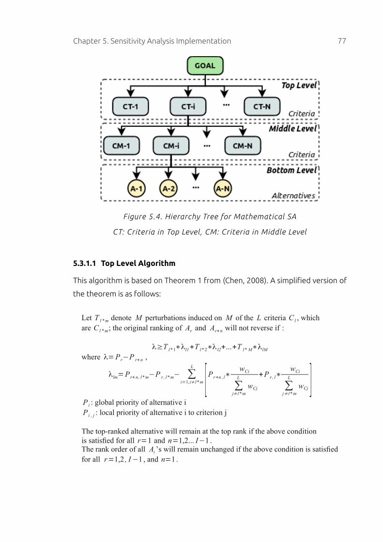
Chapter 5. Sensitivity Analysis Implementation 77
Figure 5.4. Hierarchy Tree for Mathematical SA
CT: Criteria in Top Level, CM: Criteria in Middle Level
5.3.1.1 Top Level Algorithm
This algorithm is based on Theorem 1 from (Chen, 2008). A simplified version of
the theorem is as follows:
Let T l *m denote M perturbations induced on M of the L criteria C l , which are C l *m; the original ranking of Ar and Ar+n will not reverse if :
λ≥T l *1∗λl1+T l *2∗λ l2+...+T l * M∗λlM
where λ=P r−P r+n ,
λlm=P r+ n , l *m−P r , l *m− ∑i=1, i≠l *m
L
[P r+n ,l∗wCi
∑j≠l *m
L
wCj
+P r , l∗wCi
∑j≠l *m
L
wCj ]P i : global priority of alternative iP i , j : local priority of alternative i to criterion j
The top-ranked alternative will remain at the top rank if the above conditionis satisfied for all r=1 and n=1,2... I−1 .The rank order of all Ai ’s will remain unchanged if the above condition is satisfiedfor all r=1,2 , I −1 , and n=1 .

Chapter 5. Sensitivity Analysis Implementation 78
The implemented algorithm is as follows:
Algorithm 5.5 Allowable region for top level criteria
Calculates the allowable region of perturbations where alternative Ak is the most preferred.
P: represents the global priority values of the alternatives.
E: represents the set of N elements that are being perturbed.
FOR i = 1 to NUMBER_OF_ALTERNATIVES AND i != k SET sum = 0 FOR j = 1 to N IF ej IS_NOT_IN E THEN SET PJ = RANKING of alternatives in criterion ej SET sum = sum + (PJk – PJi) * wj ENDIF ENDFOR SET S = sum / SUM(w) FOR j = 1 to N SET PJ = RANKING of alternatives in criterion ej SET ci,j = PJj – PJk + S SET Di = Pk – Pi ENDFORENDFOR
5.3.1.2 Middle Level Algorithm
This algorithm is based on Theorem 2, Corollary 2.2 from (Chen, 2008). A
simplified version of the theorem is as follows:
Let T k *ml * denote M perturbations induced on M of the K criteria C kl , which are C k *ml * (sub-criteria C k * of criterion C l * );the original ranking of Ar and Ar+n will not reverse if :
λ≥T k *1 l *∗λ k1 l+T k *2 l *∗λk2 l+...+T k *M l *∗λk M l
where λ=P r−P r+n ,
λ km l=wCl *∗[P r+n , k * m−P r , k *m+ ∑i=i ,i≠k∗m
K
(P r , i−P r+ n,i)∗wCk l *
∑j≠l *m
K
wCj l * ]The top-ranked alternative will remain at the top rank if the above condition issatisfied for all r=1 and n=1,2... I−1 .The rank order of all Ai ’s will remain unchanged if the above condition is satisfiedfor all r=1,2 , I −1 , and n=1 .
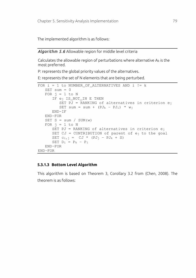
Chapter 5. Sensitivity Analysis Implementation 79
The implemented algorithm is as follows:
Algorithm 5.6 Allowable region for middle level criteria
Calculates the allowable region of perturbations where alternative Ak is the most preferred.
P: represents the global priority values of the alternatives.
E: represents the set of N elements that are being perturbed.
FOR i = 1 to NUMBER_OF_ALTERNATIVES AND i != k SET sum = 0 FOR j = 1 to N IF ej IS_NOT_IN E THEN SET PJ = RANKING of alternatives in criterion ej SET sum = sum + (PJk – PJi) * wj ENDIF ENDFOR SET S = sum / SUM(w) FOR j = 1 to N SET PJ = RANKING of alternatives in criterion ej SET CJ = CONTRIBUTION of parent of ej to the goal SET ci,j = CJ * (PJj – PJk + S) SET Di = Pk – Pi ENDFORENDFOR
5.3.1.3 Bottom Level Algorithm
This algorithm is based on Theorem 3, Corollary 3.2 from (Chen, 2008). The
theorem is as follows:

Chapter 5. Sensitivity Analysis Implementation 80
Let T i * m j * denote M perturbations induced on M of the I alternatives Aij , which are Ai *m j *(alternative Ai * under criterion C j * );the original ranking of Ar and Ar+n will not reverse if :
P r−P r+n ≥∑m=1
M
C j *∗T i *m , j *∗P r , j *−P r+n , j *
∑i=1, i≠i *
I
P i , j *
(when perturbations are induced on neither Ar , j nor Ar+n , j )
P r *−P(r+ n)* ≥(T (r+n )*m, j *−T r *m , j *)∗C j *
(when perturbations are induced on both Ar , j and Ar+n , j )
P r−P (r+n)* ≥ ∑m=1
i≠r+ n
M
[T i *m , j *∗C j *∗[P r , j *
∑i=1, i≠i *
I
P i , j * ]+T (r+n )* m, j *∗C j *∗[1+P r , j *
∑i=1, i≠i *
I
P i , j * ]](if one of the perturbations is induced on A r+ n , j )
P r *−P r+n * ≥−∑m=1i≠ r
M
[T i *m, j *∗C j *∗[P r+ n , j *
∑i=1,i≠i *
I
P i , j * ]−T r*m , j *∗C j *∗[1+P r+n , j *
∑i=1, i≠i *
I
P i , j * ]](if one of the perturbations is induced on Ar , j )
C j * : Contribution of criterion C j to the overall goal
The top-ranked alternative will remain at the top rank if the above conditionis satisfied for all r=1 and n=1,2... I−1 .The rank order of all Ai ’s will remain unchanged if the above condition is satisfiedfor all r=1,2 , I −1 , and n=1 .
The implemented algorithm is as follows:

Chapter 5. Sensitivity Analysis Implementation 81
Algorithm 5.7 Allowable region for bottom level alternatives
Calculates the allowable region of perturbations where alternative Ak is the
most preferred.
FOR i = 1 to NUMBER_OF_ALTERNATIVES AND i != k SET sum = 1 SUM(w) FOR j = 1 to N SET PJ = RANKING of alternatives in criterion ej SET CJ = CONTRIBUTION of parent of ej to the goal IF ei IS_NOT_IN E AND ek IS_NOT_IN E THEN SET ci,j = CJ * (wk – wi) / sum ELSE IF ei IS_IN E AND ek IS_IN E THEN IF k == j THEN SET ci,j = CJ ELSE SET ci,j = CJ ENDIF ELSE IF ei IS_IN E AND ek IS_NOT_IN E THEN IF i != j THEN SET ci,j = CJ * wk / sum ELSE SET ci,j = CJ * ( 1 + wk ) / sum ENDIF ELSE IF k != j THEN SET ci,j = CJ * wi / sum ELSE SET ci,j = CJ * ( 1 + wi ) / sum ENDIF ENDIF SET Di = Pk – Pi ENDFORENDFOR
The application of each of these algorithms produces a system of inequalities
similar to the one shown in formula (15) that represents the allowable range of
perturbations for an alternative to be the most preferred.
c1,1 P1+...+c1, i P i+...+c1, N PN≤D1
c2,1 P1+...+c2, i P i+...+c2,N PN ≤D2
.
.
.c N ,1 P1+...+cN ,i P i+...+c N , N P N≤DN
(15)
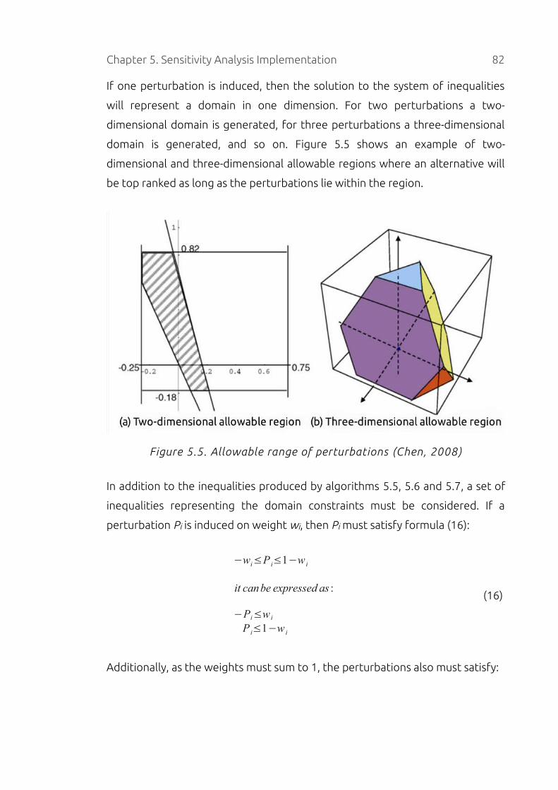
Chapter 5. Sensitivity Analysis Implementation 82
If one perturbation is induced, then the solution to the system of inequalities
will represent a domain in one dimension. For two perturbations a two-
dimensional domain is generated, for three perturbations a three-dimensional
domain is generated, and so on. Figure 5.5 shows an example of two-
dimensional and three-dimensional allowable regions where an alternative will
be top ranked as long as the perturbations lie within the region.
Figure 5.5. Allowable range of perturbations (Chen, 2008)
In addition to the inequalities produced by algorithms 5.5, 5.6 and 5.7, a set of
inequalities representing the domain constraints must be considered. If a
perturbation Pi is induced on weight wi, then Pi must satisfy formula (16):
−wi≤P i≤1−w i
it canbe expressed as :
−Pi≤w i
P i≤1−w i
(16)
Additionally, as the weights must sum to 1, the perturbations also must satisfy:

Chapter 5. Sensitivity Analysis Implementation 83
−∑ wi≤∑ P i≤1−∑w i
it canbe expressed as :
−∑ Pi≤∑ wi
∑ P i≤1−∑ w i
(17)
By executing the algorithm for each alternative and including the domain
inequalities (16) and (17), the region where each alternative is the most
preferred one can be identified by solving the system of inequalities. If one
alternative is never the most preferred, then the system of inequalities will have
no solution and the allowable region for this alternative will be empty.
5.3.1.4 Sensitivity Coefficients
In addition to the allowable region, two sensitivity coefficients can be
calculated (Chen, 2008).
• OPSC: Operating point sensitivity coefficient. It is defined as the
shortest distance from the current weights to the edge of the allowable
region. It represents the minimum change that must be induced on the
weights to cause a rank reversal.
• TSC: Total sensitivity coefficient. It is defined as the ratio of the size
(length, area, volume or hyper-volume depending on the number of
perturbations) of the allowable region of the current top alternative in
relation to the total size of the weight space. This coefficient specifies
that the shorter the allowable region is, the more sensitive the decision
problem is to variations of the weights.
5.3.2 Implementation in PriEsT
Following the general architecture of PriEsT, this SA method was implemented
first in the PriEsT library and then a front-end was designed, developed and
integrated into the main GUI of the application. This design allows the reuse of
this and the previous SA algorithms using different front-ends, as will be
Chapter 5. Sensitivity Analysis Implementation 84
discussed in the next chapter.
To make this SA method easy to use and interpret by the user, in addition to the
system of inequalities that represent the allowable region of perturbations for
each alternative, a polygon defining the boundaries of each region is also
calculated so that it can be displayed in the application. As an allowable region
will be n-dimensional when n perturbations are induced, to construct a two-
dimensional polygon, the n-dimensional allowable region is transformed or
projected into a 2-dimensional plane. Having a two-dimensional representation
of the allowable region facilitates the process of constructing a chart and more
importantly, of computing the area and shortest distance to the edges in order
to calculate the OPSC and TSC coefficients. In addition, this process replaces the
perturbation variables for the weight variables, so the resulting polygon is
easier to interpret.
The transformation is separated into four categories according to
dimensionality of the allowable region: uni-dimensional, two-dimensional,
three-dimensional and multi-dimensional.
5.3.2.1 Uni-dimensional Transformation
The system of inequalities (see Formula (15)) together with the domain
inequalities (Formulas (16) and (17)) that defines the allowable region contains
one variable, the perturbation Pi induced on the weight wi. Solving this
inequalities and replacing Pi = w'i - wi will result in:
w ' i≥aw ' i≤b (18)
To convert this result into a two-dimensional polygon, the variable w'i is mapped
on the x-axis and values for the y-axis are added in a way that the area of all the
regions will sum to 1. As a consequence, the polygon will have five points: (a,0),
(a,1), (b,1), (b,0) and (a,0). The first point is repeated to close the polygon. An
example of the resulting polygons is shown in Figure 5.6.

Chapter 5. Sensitivity Analysis Implementation 85
Figure 5.6. Uni-dimensional Projection
Figure 5.7. Two-dimensional Projection
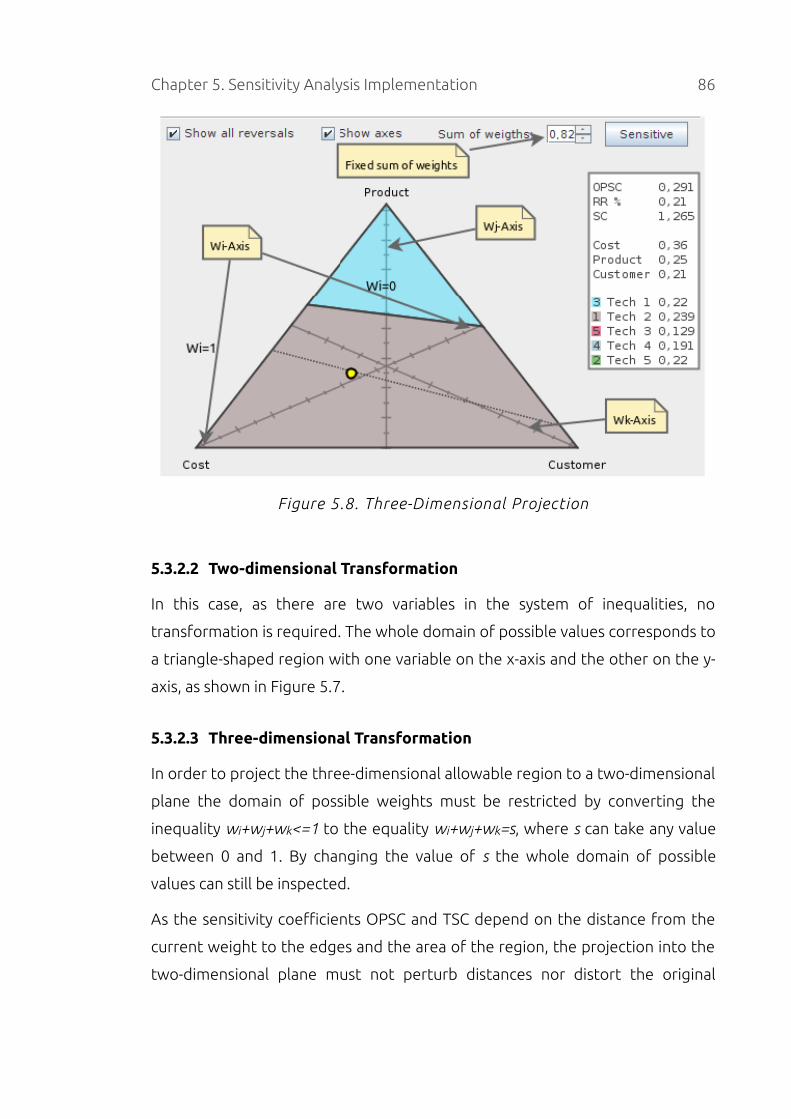
Chapter 5. Sensitivity Analysis Implementation 86
Figure 5.8. Three-Dimensional Projection
5.3.2.2 Two-dimensional Transformation
In this case, as there are two variables in the system of inequalities, no
transformation is required. The whole domain of possible values corresponds to
a triangle-shaped region with one variable on the x-axis and the other on the y-
axis, as shown in Figure 5.7.
5.3.2.3 Three-dimensional Transformation
In order to project the three-dimensional allowable region to a two-dimensional
plane the domain of possible weights must be restricted by converting the
inequality wi+wj+wk<=1 to the equality wi+wj+wk=s, where s can take any value
between 0 and 1. By changing the value of s the whole domain of possible
values can still be inspected.
As the sensitivity coefficients OPSC and TSC depend on the distance from the
current weight to the edges and the area of the region, the projection into the
two-dimensional plane must not perturb distances nor distort the original
Chapter 5. Sensitivity Analysis Implementation 87
shape of the region. Erkut and Tarimcilar (Erkut, 1991) proposed a method for
finding the boundaries of each region and projecting the three-dimensional
region into a two-dimensional plane with no distortion of images. This method
allows the weights to be converted from a three-dimensional point (wi, wj, wk)
into a two-dimensional point (x,y) and vice-versa.
As shown in Figure 5.8, the user is allowed to change the value of s (sum of
weights) to inspect the sensitivity of the model for all possible combinations of
the three weights. In each corner of the triangle, one of the weights has a value
of s and the others 0 and in the middle of the base, one of the weights is 0 and
the other two are s/2.
5.3.2.4 Multi-dimensional Transformation
This transformation was not implemented because further research is needed
to investigate how a multi-dimensional polytope with 4 or more dimensions can
be represented in a two-dimensional plane. Because of time constraints, a
research on this matter is beyond the scope of the project and will be
presented as future work in Chapter 8.
5.3.2.5 Sensitivity Coefficients and Rank Reversal
The implemented SA module presents three coefficients to the user: OPSC, RR
% (Rank Reversal Probability) and SC (Sensitivity Coefficient), as shown in
Figures 5.6, 5.7 and 5.8.
As TSC represents the ratio of the area of the top alternative's allowable region
to the total area, then 1-TSC will represent the probability that a rank reversal
occurs for any combination of weights. That is, if TSC is close to 0, then 1-TSC
will be close to 1 and vice-versa. 1-TSC was named Rank Reversal Probability and
is presented as RR%.
In a similar way, SC=1/TSC is more meaningful, as a small value of SC will
indicate a low sensitivity to changes in the weight while a large value of SC will
indicate that the problem is very sensitive to changes to the relative importance
of criteria.

Chapter 5. Sensitivity Analysis Implementation 88
Additionally, if a rank reversal occurs for some combination of weights but it
does not change the top alternative, it is included in the charts as a dotted line.
Secondary rank reversals are displayed in Figures 5.6, 5.7 and 5.8.
5.3.2.6 Most Sensitive Decision Element
The element (or set of elements as up to three elements may be selected) with
the lowest OPSC and TSC can be considered as the most sensitive decision
element. If the lowest OPSC and TSC belong to different elements, then the
element with the lowest OPSC * TSC can be considered to be the most sensitive.
In order to locate this element, an SA is performed at each node of the decision
problem and the OPSC and TSC values are recorded. The analysis is done using
all possible combinations of the child nodes in groups of one, two and three
elements. The total number of different combinations for a node with n child
elements is given in formula (19):
combinations=n+n !
(n−2)! 2!+
n !(n−3)! 3 !
(19)
Once all nodes are analysed, two decision elements are identified: the element
with the lowest OPSC and the one that obtained the lowest TSC. If these are
different elements, then the element with the lowest OPSC * TSC is considered
as the most sensitive element of the decision problem.
5.3.3 Advantages
Some of the advantages of the mathematical modelling method are as follows:
• Simple to use and interpret. Usage of the SA method is relatively
simple, the user only has to select from one to three elements from the
decision problem and the allowable regions are plotted automatically
presenting the sensitivity of the decision elements in a visual way . The
chart is interactive as it allows the user to select any point inside the
polygon to obtain the associated ranking of alternatives.

Chapter 5. Sensitivity Analysis Implementation 89
• Fast response time. The algorithm has no execution loops hence it
has relatively fast execution. The chart is updated instantly after the user
selects the decision elements.
• Sensitivity coefficients: Three sensitivity coefficients (OPSC, RR%
and SC) and the most sensitive decision element are presented to the
user.
5.3.4 Limitations
Some of the limitations of the mathematical modelling method are as follows:
• Chart available for up to three elements . This method allows any
number of decision elements to be analysed, however, the visualisation
of the results in a chart is limited to three elements. More research is
necessary to find a method for displaying results when more than three
elements are considered.
5.4 Select a Single Solution from PrInT
The optimisation-based method PrInT (Siraj, 2011) generates more than one
non-dominated solution from a PC matrix. Automated selection of a single
solution was suggested as an area for further work by Siraj (Siraj, 2011) and is
widely regarded as a major challenge in the area. By using the implemented
mathematical SA method a single solution can be selected from the set of non-
dominated solutions by choosing the solution that minimises the sensitivity of
the final ranking of alternatives.
A decision problem may have any number of decision elements and for each
element PrInT produces a set of solutions. For each solution an SA is conducted
to find the most sensitive element and its associated OPSC value. The solution
that generates the most sensitive element with the highest OPSC value can be
selected as the best solution for that decision element, as that solution
produces the most robust final ranking of alternatives.
This novel method has been implemented in PriEsT as represented in Algorithm
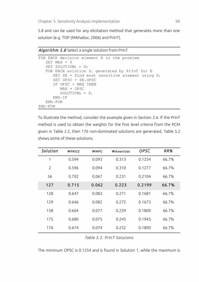
Chapter 5. Sensitivity Analysis Implementation 90
5.8 and can be used for any elicitation method that generates more than one
solution (e.g. TOP (Mikhailov, 2006) and PrInT).
Algorithm 5.8 Select a single solution from PrInT
FOR EACH decision element E in the problem SET MAX = 0 SET SOLUTIONE = S0 FOR EACH solution Si generated by PrInT for E SET SE = find most sensitive element using Si SET OPSC = SE.OPSC IF OPSC > MAX THEN MAX = OPSC SOLUTIONE = Si ENDIF ENDFORENDFOR
To illustrate the method, consider the example given in Section 2.6. If the PrInT
method is used to obtain the weights for the first level criteria from the PCM
given in Table 2.2, then 176 non-dominated solutions are generated. Table 5.2
shows some of these solutions.
Solution wPRICE wMPG wAmenities OPSC RR%
1 0.594 0.093 0.313 0.1254 66.7%
2 0.596 0.094 0.310 0.1277 66.7%
56 0.702 0.067 0.231 0.2104 66.7%
127 0.715 0.062 0.223 0.2199 66.7%
128 0.647 0.083 0.271 0.1681 66.7%
129 0.646 0.082 0.272 0.1673 66.7%
158 0.664 0.077 0.259 0.1809 66.7%
175 0.680 0.075 0.245 0.1943 66.7%
176 0.674 0.074 0.252 0.1890 66.7%
Table 5.2. PrInT Solutions
The minimum OPSC is 0.1254 and is found in Solution 1, while the maximum is

Chapter 5. Sensitivity Analysis Implementation 91
0.2199 and is found in solution 127. By choosing solution 127, the minimum
change of weights necessary to cause a rank reversal is 0.2199 which represents
a 75.4% more robust ranking than solution 1.
By using this approach for selecting a single solution from elicitation methods
that generate more than one, the final ranking of alternatives is more robust to
changes in criteria weights giving the DM more confidence about the suggested
ranking.
5.5 Case Study: Supplier Selection Problem
A recent study (Bruno, 2012) that focuses on the supplier selection problem
(SSP) will be used to demonstrate the features of the three SA methods. The
study uses AHP to construct a model to evaluate suppliers in order to improve a
firm's competitiveness.
The model contains two levels of criteria. The first level includes process and
product quality (PPQ), service level (SL), management and innovation (MI), and
financial position (FP). The weights for these four criteria are:
wPPQ = 41.7%, wSL = 35.9%, wMI = 9.5%, wFP = 13%
Each of these criteria contains three sub-criteria, as shown in Figure 5.9. There
are four supplier companies under consideration: alpha, beta, gamma and delta.
The final weights calculated using either the EV or GM method are:
walpha = 24.6%, wbeta = 29.8%, wgamma = 21.3%, wdelta = 24.2%
The most preferred alternative is beta with a weight of 29.8%, followed by
alpha and delta with a weight of 24.6% and 24.2% respectively.
5.5.1 Sensitivity Analysis using PriEsT
The decision problem is first analysed using the probabilistic simulation
approach. By using the random generator the likely rank order of the
alternatives may be identified independently from criteria weights.

Chapter 5. Sensitivity Analysis Implementation 92
Figure 5.9. AHP model for supplier selection
Figure 5.10a shows the ranking of alternatives when uniformly distributed
random weights are used for the top-level criteria (PPQ, SL, MI and FP). Supplier
beta has a mean ranking around 1.25 with the best ranking of 1 and the worst
as 4. In the 50% of the simulation iterations (quartile1 and quartile3), beta was
top ranked. Supplier alpha had a mean ranking of 2.2, with best and worst
rankings of 1 and 3 respectively. Although gamma and delta are ranked
between 3rd and 4th half of the time, for some combination of weights they
become the top ranked alternative.
The simulation was executed again replacing all criteria weights with random
weights, as shown in Figure 5.10b. This time beta is still the best alternative,
however gamma, which was the worst alternative with 21.3%, now is in second
place with a mean ranking of 2.5 and a ranking between 1 and 4 for 50% of the
iterations. Similar results are obtained using the gamma or triangular
distribution.
Given this scenario each alternative has to be considered in the further analysis
as each may be the most preferred for some combination of weights.

Chapter 5. Sensitivity Analysis Implementation 93
Figure 5.10. Ranking of alternatives using probabilistic simulation
To discover what weights cause the ranking to change, the one-at-a-time and
mathematical analyses are performed. The one-at-a-time method shows that a
decrease in the weight of PPQ from 41.6% to 12.2% causes gamma to be the
preferred alternative with a priority of 25.8%, as shown in Figure 5.11. Similarly,
for weights of SL in the interval 53.8% to 55.4% alpha is the best alternative,
and from 55.4% to 100% gamma is the most preferred supplier.
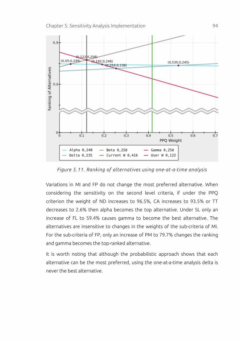
Chapter 5. Sensitivity Analysis Implementation 94
Figure 5.11. Ranking of alternatives using one-at-a-time analysis
Variations in MI and FP do not change the most preferred alternative. When
considering the sensitivity on the second level criteria, if under the PPQ
criterion the weight of ND increases to 96.5%, CA increases to 93.5% or TT
decreases to 2.6% then alpha becomes the top alternative. Under SL only an
increase of FL to 59.4% causes gamma to become the best alternative. The
alternatives are insensitive to changes in the weights of the sub-criteria of MI.
For the sub-criteria of FP, only an increase of PM to 79.7% changes the ranking
and gamma becomes the top-ranked alternative.
It is worth noting that although the probabilistic approach shows that each
alternative can be the most preferred, using the one-at-a-time analysis delta is
never the best alternative.

Chapter 5. Sensitivity Analysis Implementation 95
Figure 5.12. Ranking of alternatives using the mathematical SA
Three simultaneous changes were considered when using the mathematical
analysis. Figure 5.12 shows the charts generated when the first level criteria is
analysed and the most sensitive element identified by PriEsT. The sensitivity
coefficients for each chart are presented in Table 5.3.
The lowest OPSC is present in chart (d), however the rank reversal probability is
just 2%. The most sensitive element, represented by chart (e), corresponds to
the SL criterion with OPSC and RR% of 0.180 and 46.3% respectively. In other
words, the smallest change to produce a rank reversal and cause delta to be the
most preferred alternative is found in (d), although (e) represents a higher
probability of rank reversal when the criteria weights are perturbed.

Chapter 5. Sensitivity Analysis Implementation 96
Chart OPSC RR% SC
(a) 0.257 14.7% 1.172
(b) 0.184 16.9% 1.203
(c) 0.544 0% 1
(d) 0.174 2% 1.102
(e) 0.180 46.3% 1.861
Table 5.3. Sensitivity coefficients
Chart (b) represents all the combinations of weights of PPQ, SL and FP while
the weight of MI is kept constant at its original value of 9.5%, hence, the sum of
PPQ, SL and FP is fixed at 90.5%. When FP and PPQ are decreased and MI is
increased, gamma, alpha and delta may become the most preferred
alternatives. By interacting with the chart, the combination of weights that
cause a rank reversal can be identified. Table 5.4 shows an example of this
situation.
PPQ SL MI FP #1 #2 #3 #4
0.416 0.358 0.095 0.131 beta 0.298 alpha 0.246 delta 0.242 gamma 0.213
0.281 0.550 0.095 0.073 alpha 0.252 delta 0.251 gamma 0.250 beta 0.246
0.308 0.555 0.095 0.041 delta 0.255 alpha 0.253 gamma 0.249 beta 0.243
0.245 0.550 0.095 0.110 gamma 0.253 alpha 0.251 beta 0.249 delta 0.246
Table 5.4. Ranking of suppliers with different weight combinations
Performing the same analysis for the second-level criteria, the most significant
result is when PU, FL and PF (sub-criteria of SL) are analysed. For this triple,
OPSC is 0.477 and RR% is 16.6% and gamma may become the first alternative if
PU and PF are decreased and FL is increased.
5.6 Summary
This chapter has discussed the design and implementation of three different
methods for performing SA. In addition, a brief discussion on the advantages

Chapter 5. Sensitivity Analysis Implementation 97
and limitations of each method was presented. The one-at-a-time method
provides a fast and easy to use approach for analysing a decision problem,
however, only one perturbation can be analysed. The simulation technique
allows the decision maker to investigate the ranking of alternatives when the
weights of any number of decision elements are modified. This approach has
proven to be useful to analyse a problem exploring all possible combinations of
weights in all levels of the hierarchy. The mathematical algorithm can analyse
any number of decision elements in the same level of the hierarchy and also
presents three sensitivity coefficients (OPSC, RR% and SC), however, only up to
three elements can be visualised in chart format. The projection of the three-
dimensional allowable region into a two-dimensional region provides the user
with an easy tool to interpret the results.
In addition, the problem of selecting a single solution from a set of non-
dominated solutions generated from the input judgements has been achieved
via a novel method that uses the mathematical SA algorithm and sensitivity
coefficients.
The chapter ends with the presentation of a SSP (supplier selection problem)
case study. The use of the three SA methods allows investigation of each
possible scenario where the rank of the best alternative may be reversed. The
analysis has shown the usefulness of inspecting the problem with different SA
methods. The probabilistic approach showed that each alternative may be the
most preferred, although two of them were more likely to be selected. Further
analysis was carried out with the one-at-a-time and mathematical algorithms to
determine under what conditions the ranking of alternatives may be modified.
Chapter 6
Platform Portability
This chapter discusses the process of porting PriEsT to web and mobile
platforms. The web platform was covered by developing a Java applet whilst
for the mobile platform two versions were created, one for J2ME-enabled
devices and one for the Android operating system. The chapter ends by
discussing briefly the challenges faced during the implementation process.
Specific tests and evaluation of these versions are presented in Chapter 7.
6.1 Portability Context
In recent years, there has been an increasing interest in web applications with
examples such as Google family of web applications, Microsoft Office 365,
social networks, media, and many others. Similarly, mobile phones are
increasingly being equipped with more processing power, memory and
functionality. At the same time, they are becoming the main computing device
for many users. Individuals carry them most of the time, and in areas of field
activity such as sales and technical support, smart phones are gradually
replacing the use of laptops.
There appears a natural evolution of tool provision on web and mobile
platforms; however this is not yet apparent in MCDM and AHP software. Whilst
several tools support AHP and PC as discussed in Section 3.2, only Web-HIPRE
(Mustajoki, 2000), MakeItRational (MakeItRational, 2012) and V.I.S.A. (SIMUL8,
2012) are web-based (other tools only support Windows); there appears to exist
no mobile version of AHP software other than the version developed here.
The re-engineering process carried out in the PriEsT tool and the architecture
design choices detailed in Chapter 4 enables a relatively simple implementation
of both a Java applet and a J2ME mobile version by re-using the PriEsT library
and implementing a user interface for the mobile platform, as Java applets can
reuse the Swing user interface of a desktop application. In addition, as the
98
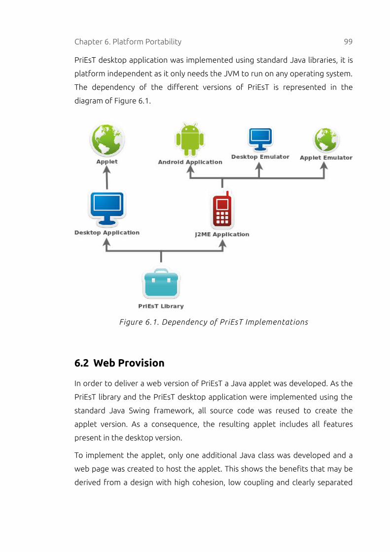
Chapter 6. Platform Portability 99
PriEsT desktop application was implemented using standard Java libraries, it is
platform independent as it only needs the JVM to run on any operating system.
The dependency of the different versions of PriEsT is represented in the
diagram of Figure 6.1.
Figure 6.1. Dependency of PriEsT Implementations
6.2 Web Provision
In order to deliver a web version of PriEsT a Java applet was developed. As the
PriEsT library and the PriEsT desktop application were implemented using the
standard Java Swing framework, all source code was reused to create the
applet version. As a consequence, the resulting applet includes all features
present in the desktop version.
To implement the applet, only one additional Java class was developed and a
web page was created to host the applet. This shows the benefits that may be
derived from a design with high cohesion, low coupling and clearly separated

Chapter 6. Platform Portability 100
concerns.
In order to test the applet, it was published in the personal pages website
available in the School of Computer Science network7. The same set of tests
used to evaluate the desktop application were executed to evaluate the applet,
these tests are included in Appendix B.
6.3 Mobile Provision
6.3.1 J2ME Port
A mobile version of PriEsT was implemented for the J2ME platform allowing
PriEsT to be run on any mobile device that supports MIDP.
The design and creation of the user-interface was done using the LWUIT toolkit.
This approach has the advantage of decoupling the user-interface from the
source code, that is, modifications to the GUI may be made without changing
the code of the application.
Figure 6.2. Package Diagram for PriEsT Mobile
7 Currently the applet is available online at: http://www2.cs.man.ac.uk/~bertuzzr/

Chapter 6. Platform Portability 101
Additionally, by using LWUIT the implementation process can be focused on the
application logic rather than on GUI components.
In addition, LWUIT takes care of the implementation-specific issues on each
mobile platform such as screen size, memory, APIs, hardware keys, touch
screens, etc. resulting in an application that will have the same look and feel on
any device, as can be seen on Figure 6.3.
The architecture of the mobile application is similar to the architecture of the
desktop application, using the MVC pattern. The PriEsT library was used as the
model of the architecture; the GUI was designed end implemented
independently using the LWUIT toolkit; and a controller class was implemented
to manage the interaction between the GUI and the PriEsT library.
Figure 6.3. PriEsT Mobile
In addition to the J2ME mobile version, two other applications were also
developed on top of the mobile version. LWUIT also supports Java SE, hence
the controller and GUI were reused to implement both a desktop and an applet

Chapter 6. Platform Portability 102
version of the mobile application. In this way, the mobile version can be tested
and tried with no need for a real device. The architecture design is shown in a
simplified form in Figure 6.2 while the layout of this dependency is represented
in Figure 6.1.
6.3.2 Limitations
A set of features present in PriEsT were removed from the mobile application
because of screen size constraints and usability. These features are the graph
view, equaliser view and visualising multiple results from methods.
The graph view presents the PC matrix as a graph allowing the user to inspect
the intransitive judgements and cycles, but it requires significant space in the
screen to draw all nodes, lines and weights, hence, it was removed from the
mobile version.
The equaliser view presents the PC matrix as a list of pairwise comparisons
allowing the decision maker to inspect the the inconsistency between direct
and indirect judgements. For the same reason as above, this feature has been
left out of the mobile version.
The last missing feature is the list of all results elicited from a method,
especially the optimisation methods. When a method produces more than one
result, the mobile version automatically picks the first result and ignores the
rest. In order to show all results, which may be as many as hundreds, a large list
would be required but in a mobile device such a big list may be cumbersome to
use and clutter the user interface.
6.3.3 Android Port
PriEsT Mobile was also ported to the Android platform. Although Android does
not support J2ME, it does support Java and, fortunately, LWUIT also supports
Android. In order to create the Android port, PriEsT was compiled using the
Android SDK and tested using an emulator and a real device (Samsung Galaxy
SII). No modifications were necessary, as the architecture of PriEsT allowed a
straightforward compilation and creation of an installer package.
Chapter 6. Platform Portability 103
6.4 Challenges faced in the implementation
The PriEsT library uses two external libraries, Jama and JMetal. Jama is used to
work with matrices while JMetal is used for implementing the optimisation-
based elicitation methods. JMetal is incompatible with J2ME as it uses some
Java libraries8 not present in the J2ME platform. For this reason, it was
necessary to modify the source code of the library and remove these
dependencies.
The source code of the library was analysed and 30 classes were identified as
required, directly or indirectly, by PriEsT. Each of these classes was analysed in
more detail, external dependencies were removed and then ported to J2ME. To
be able to make this port, the tool Retrotranslator was used to back-port the
source code from the Java 1.6 version back to the 1.4, which is the version that
J2ME supports. In addition, the “java.util” library was also back-ported as it was
required both by JMetal and PriEsT. With JMetal and “java.util” ported to J2ME,
the optimisation-based methods can be included in PriEsT Mobile.
6.5 Summary
This chapter has discussed the implementation process for porting PriEsT to
web and mobile platforms. A brief introduction and motivation were presented
and then the web provision was discussed. Next, the architecture for the mobile
version of PriEsT was presented and the implementation details of the J2ME
and Android version were introduced. The chapter ends describing the
challenges and problems faced during this implementation process and they
were handled.
8 Some of these libraries include java.util (for using lists, arrays, sorting, etc.) and java.io (for
file input/output).

Chapter 7
Project Evaluation
This chapter presents the evaluation of the sensitivity analysis methods and the
platform-specific versions of PriEsT. Although testing was conducted
throughout the project to ensure the methods and software were correctly
implemented (a list of all the tests may be found in Appendix B), a high-level
evaluation was performed to obtain indicators about the completeness and
performance of the implementation.
7.1 Evaluation of PriEsT
The evaluation of PriEsT was separated into three categories: requirements,
performance and portability.
7.1.1 Requirements
The aim of this evaluation section is to produce a traceability matrix that
presents the level of fulfilment of the new requirements and also to
demonstrate that all the original features of PriEsT were included in the new
version after the re-engineering process.
A system testing was performed against the original requirements (Siraj, 2011)
and the new requirements covered in Section 4.3 for PriEsT.
Figure B.1 in Appendix B contains a list of the tests performed when PriEsT was
first developed by Siraj. These tests were executed against the new versions of
PriEsT, desktop and mobile, to certify that all original features are still present
in this version.
A brief discussion of the tests that have been ignored, failed or that produced
different results as the original plan is given next. Tests that passed in the
original plan and passed in the new version are omitted.
• T1-0003. This test is to evaluate group decision making (GDM). The
104

Chapter 7. Project Evaluation 105
original version of PriEsT does not support GDM, as a consequence this
test have failed in the original test plan. As GDM was not included as a
new requirement in the new version, this test was omitted.
• T1-0006. This test have passed for the desktop application but was
omitted for the mobile application as graph view was not implemented
as discussed in Section 6.3.2.
• T1-0008. This test evaluates the support for remote input of
judgements for GDM. As GDM was not included as a new requirement in
the new version, this test was omitted.
• T1-0009. Displaying congruence and dissonance measures in the PCM
was not implemented in the mobile version as discussed in Section 6.3.2,
hence, this test was omitted.
• T1-0011 and T1-0012. These tests evaluates the support for
highlighting the most inconsistent triple and three-way cycles. For the
same reason given above, these tests were omitted for the mobile
version of PriEsT.
• T1-0015 and T1-0016. These tests have passed for the desktop
application and have been omitted for the mobile version. The mobile
application automatically selects the first result when an elicitation
method produces more than one results for a PCM, as a consequence,
the mobile version does not include a chart for plotting results in the TD-
NV and TD-TD2 space.
• T1-0020. This test, for evaluating support for a web-based application,
was failed in the original test plan but have now passed as a web version
of PriEsT has been implemented.
• T1-0023. Similarly as test T1-0020, this test was failed before but have
now passed as a mobile version of PriEsT has been developed.
Table 7.1 shows the results of the system testing performed against the new
requirements for PriEsT. All requirements have been fully implemented and
tested, although non-functional requirement NR-005 is marked as partial as not
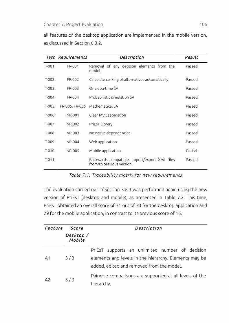
Chapter 7. Project Evaluation 106
all features of the desktop application are implemented in the mobile version,
as discussed in Section 6.3.2.
Test Requirements Description Result
T-001 FR-001 Removal of any decision elements from the model
Passed
T-002 FR-002 Calculate ranking of alternatives automatically Passed
T-003 FR-003 One-at-a-time SA Passed
T-004 FR-004 Probabilistic simulation SA Passed
T-005 FR-005, FR-006 Mathematical SA Passed
T-006 NR-001 Clear MVC separation Passed
T-007 NR-002 PriEsT Library Passed
T-008 NR-003 No native dependencies Passed
T-009 NR-004 Web application Passed
T-010 NR-005 Mobile application Partial
T-011 - Backwards compatible. Import/export XML files from/to previous version.
Passed
Table 7.1. Traceability matrix for new requirements
The evaluation carried out in Section 3.2.3 was performed again using the new
version of PriEsT (desktop and mobile), as presented in Table 7.2. This time,
PriEsT obtained an overall score of 31 out of 33 for the desktop application and
29 for the mobile application, in contrast to its previous score of 16.
F e a t u r e S c o r e
D e s k t o p / M o b i l e
D e s c r i p t i o n
A1 3 / 3
PriEsT supports an unlimited number of decision
elements and levels in the hierarchy. Elements may be
added, edited and removed from the model.
A2 3 / 3Pairwise comparisons are supported at all levels of the
hierarchy.
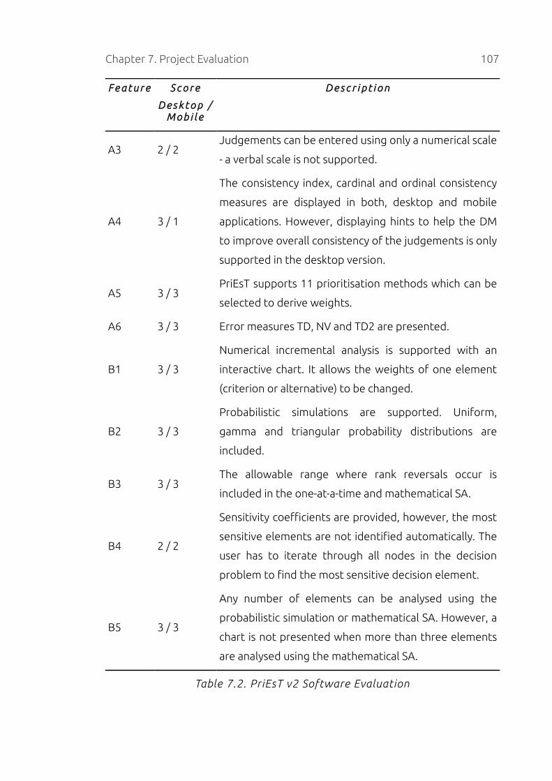
Chapter 7. Project Evaluation 107
F e a t u r e S c o r e
D e s k t o p / M o b i l e
D e s c r i p t i o n
A3 2 / 2Judgements can be entered using only a numerical scale
- a verbal scale is not supported.
A4 3 / 1
The consistency index, cardinal and ordinal consistency
measures are displayed in both, desktop and mobile
applications. However, displaying hints to help the DM
to improve overall consistency of the judgements is only
supported in the desktop version.
A5 3 / 3PriEsT supports 11 prioritisation methods which can be
selected to derive weights.
A6 3 / 3 Error measures TD, NV and TD2 are presented.
B1 3 / 3
Numerical incremental analysis is supported with an
interactive chart. It allows the weights of one element
(criterion or alternative) to be changed.
B2 3 / 3
Probabilistic simulations are supported. Uniform,
gamma and triangular probability distributions are
included.
B3 3 / 3The allowable range where rank reversals occur is
included in the one-at-a-time and mathematical SA.
B4 2 / 2
Sensitivity coefficients are provided, however, the most
sensitive elements are not identified automatically. The
user has to iterate through all nodes in the decision
problem to find the most sensitive decision element.
B5 3 / 3
Any number of elements can be analysed using the
probabilistic simulation or mathematical SA. However, a
chart is not presented when more than three elements
are analysed using the mathematical SA.
Table 7.2. PriEsT v2 Software Evaluation
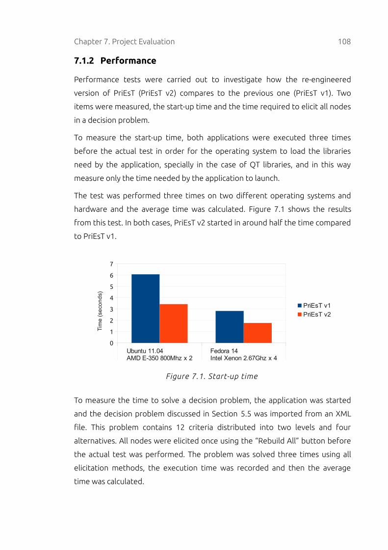
Chapter 7. Project Evaluation 108
7.1.2 Performance
Performance tests were carried out to investigate how the re-engineered
version of PriEsT (PriEsT v2) compares to the previous one (PriEsT v1). Two
items were measured, the start-up time and the time required to elicit all nodes
in a decision problem.
To measure the start-up time, both applications were executed three times
before the actual test in order for the operating system to load the libraries
need by the application, specially in the case of QT libraries, and in this way
measure only the time needed by the application to launch.
The test was performed three times on two different operating systems and
hardware and the average time was calculated. Figure 7.1 shows the results
from this test. In both cases, PriEsT v2 started in around half the time compared
to PriEsT v1.
Ubuntu 11.04AMD E-350 800Mhz x 2
Fedora 14Intel Xenon 2.67Ghz x 4
0
1
2
3
4
5
6
7
PriEsT v1
PriEsT v2
Tim
e (
seco
nd
s )
Figure 7.1. Start-up time
To measure the time to solve a decision problem, the application was started
and the decision problem discussed in Section 5.5 was imported from an XML
file. This problem contains 12 criteria distributed into two levels and four
alternatives. All nodes were elicited once using the “Rebuild All” button before
the actual test was performed. The problem was solved three times using all
elicitation methods, the execution time was recorded and then the average
time was calculated.
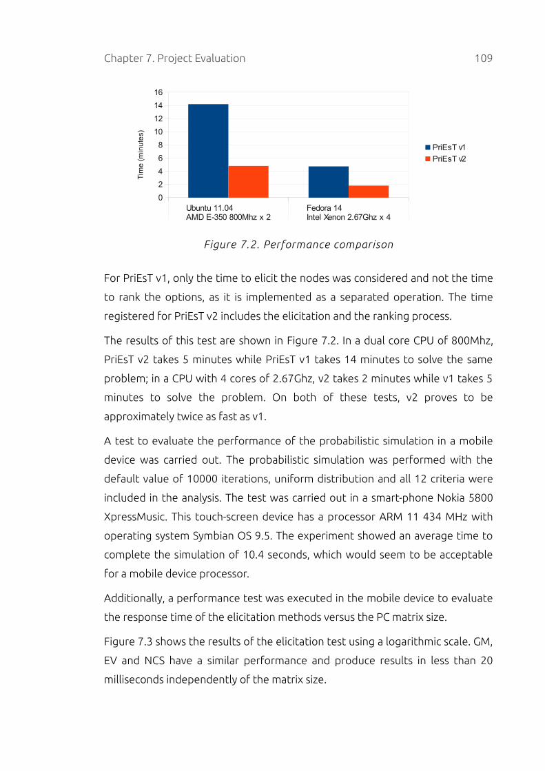
Chapter 7. Project Evaluation 109
Ubuntu 11.04AMD E-350 800Mhz x 2
Fedora 14Intel Xenon 2.67Ghz x 4
0
2
4
6
8
10
12
14
16
PriEsT v1
PriEsT v2
Tim
e (
min
ute
s)
Figure 7.2. Performance comparison
For PriEsT v1, only the time to elicit the nodes was considered and not the time
to rank the options, as it is implemented as a separated operation. The time
registered for PriEsT v2 includes the elicitation and the ranking process.
The results of this test are shown in Figure 7.2. In a dual core CPU of 800Mhz,
PriEsT v2 takes 5 minutes while PriEsT v1 takes 14 minutes to solve the same
problem; in a CPU with 4 cores of 2.67Ghz, v2 takes 2 minutes while v1 takes 5
minutes to solve the problem. On both of these tests, v2 proves to be
approximately twice as fast as v1.
A test to evaluate the performance of the probabilistic simulation in a mobile
device was carried out. The probabilistic simulation was performed with the
default value of 10000 iterations, uniform distribution and all 12 criteria were
included in the analysis. The test was carried out in a smart-phone Nokia 5800
XpressMusic. This touch-screen device has a processor ARM 11 434 MHz with
operating system Symbian OS 9.5. The experiment showed an average time to
complete the simulation of 10.4 seconds, which would seem to be acceptable
for a mobile device processor.
Additionally, a performance test was executed in the mobile device to evaluate
the response time of the elicitation methods versus the PC matrix size.
Figure 7.3 shows the results of the elicitation test using a logarithmic scale. GM,
EV and NCS have a similar performance and produce results in less than 20
milliseconds independently of the matrix size.
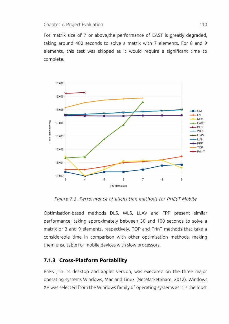
Chapter 7. Project Evaluation 110
For matrix size of 7 or above,the performance of EAST is greatly degraded,
taking around 400 seconds to solve a matrix with 7 elements. For 8 and 9
elements, this test was skipped as it would require a significant time to
complete.
3 4 5 6 7 8 91E+00
1E+01
1E+02
1E+03
1E+04
1E+05
1E+06
1E+07
GM
EV
NCS
EAST
DLS
WLS
LLAV
LLS
FPP
TOP
PriInT
PC Matrix size
Tim
e (
mill
ise
con
ds)
Figure 7.3. Performance of elicitation methods for PriEsT Mobile
Optimisation-based methods DLS, WLS, LLAV and FPP present similar
performance, taking approximately between 30 and 100 seconds to solve a
matrix of 3 and 9 elements, respectively. TOP and PrInT methods that take a
considerable time in comparison with other optimisation methods, making
them unsuitable for mobile devices with slow processors.
7.1.3 Cross-Platform Portability
PriEsT, in its desktop and applet version, was executed on the three major
operating systems Windows, Mac and Linux (NetMarketShare, 2012). Windows
XP was selected from the Windows family of operating systems as it is the most

Chapter 7. Project Evaluation 111
used version as of 2012 (NetMarketShare, 2012); for Max and Linux, Mac OS X
v10 and Ubuntu Linux 11.04 were selected.
A decision problem aimed at evaluating emerging technologies in the
semiconductor industry (Chen, 2009) was selected to test PriEsT on the three
operating systems. The problem was loaded from an XML file, solved and then
analysed using SA.
In the three platforms, the results were the same and all features worked
properly. Appendix D contains screen-shots of PriEsT running on each operating
system.
7.2 Evaluation of Sensitivity Analysis
In order to evaluate the SA methods, two analyses were carried out: a
performance test and a comparison evaluation to investigate the accuracy of
the algorithms in identifying rank reversals.
To perform these tests, two Monte-Carlo simulations were executed. In the first
simulation, for each iteration a decision problem was created with n criteria,
ranging from 3 to 12, and 9 alternatives9. In the second simulation, the number
of criteria was fixed at 9, and the alternatives ranged from 3 to 12. In both
simulations, 3000 problems where generated for each iteration; all judgements
were generated randomly using the scale 1-9.
For each iteration, the problem was solved using the GM method and then an
SA (using all three methods) was conducted on the criteria weights. For the
probabilistic simulation algorithm, the default 10000 uniform random
simulations were used. The execution time and results from each SA algorithm
were recorded and are analysed next.
7.2.1 Performance
The average time was calculated from the results of the Monte-Carlo
9 Saaty (Saaty, 1977) defined 9 as the limit for any PC matrix based on a cognitive limitation of
the mind which cannot handle more than 7±2 simultaneous comparisons.

Chapter 7. Project Evaluation 112
simulations to compare the execution time of each SA method. The test was
performed on a machine with an Intel Core 2 Duo CPU running at 3.00GHz.
Figure 7.4. Computation time for SA methods
Figure 7.4a shows the results of the test with 9 alternatives and the number of
criteria ranging from 3 to 12, while Figure 7.4b gives results for the simulation
when the number of criteria is fixed at 9 and alternatives range from 3 to 12.
One-at-a-time and mathematical methods take the lowest amount of
computational time, below 3 milliseconds, and appear to be insensitive to the
number of alternatives or criteria.
The probabilistic approach takes more processing time than the other two
methods and shows a linear relation between the number of alternatives or
Chapter 7. Project Evaluation 113
criteria and the computation time. However, the time required to perform SA
using this method is still relatively low, as approximately 22 milliseconds were
required to perform a probabilistic simulation with 12 criteria and 9
alternatives, as shown in Figure 7.4a.
The impressively low time for the probabilistic simulation algorithm, which
performed 10000 simulations, may be explained by the fact that a warm-up
session was executed before the actual test. This session consisted in running
one Monte-Carlo iteration to allow the JVM to load all the classes necessary to
prevent the time used by the class-loader to affect the results. This session may
have triggered the JIT compiler to compile the code of the probabilistic
algorithm into native code causing an increase in the performance.
7.2.2 Methods Comparison
This analysis was carried out to compare how the three SA algorithms behave
when finding rank reversal conditions.
For each iteration of the Monte-Carlo simulations the ranking of alternatives
was calculated and the three SA algorithms were executed. As the output of
the algorithms cannot be compared directly as they produce different kind of
results, the analysis focused on finding how many alternatives may be the most
preferred according to each algorithm.
Under this analysis, the most effective algorithm is the one that finds the
highest number of rank reversals that causes the top-ranked alternative to
change. Rank reversals between other alternatives are ignored.
Figure 7.5 gives the results of the simulation. The y-axis represents the number
of rank reversals while the x-axis represent the number of criteria (Figure 7.5a)
and number of alternatives (Figure 7.5b). As the simulation was repeated 3000
times for each value of the x-axis, the indicators minimum, maximum, quartile 1,
quartile 3 and mean were calculated.
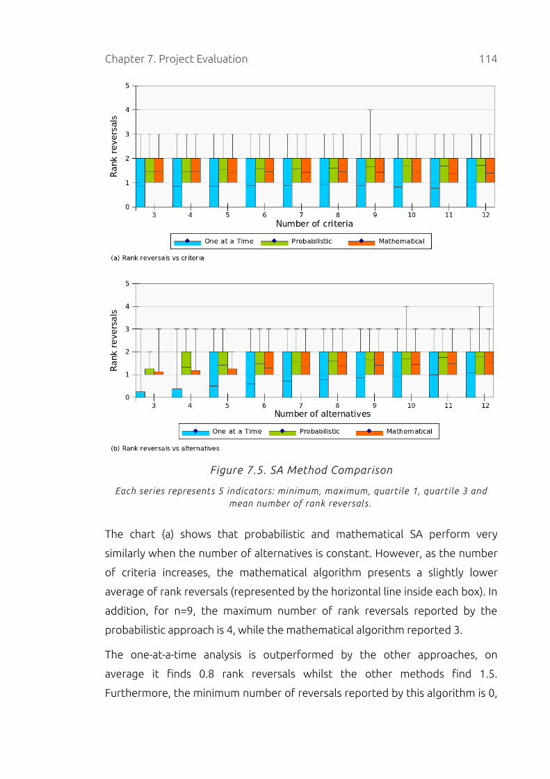
Chapter 7. Project Evaluation 114
Figure 7.5. SA Method Comparison
Each series represents 5 indicators: minimum, maximum, quartile 1, quartile 3 and mean number of rank reversals.
The chart (a) shows that probabilistic and mathematical SA perform very
similarly when the number of alternatives is constant. However, as the number
of criteria increases, the mathematical algorithm presents a slightly lower
average of rank reversals (represented by the horizontal line inside each box). In
addition, for n=9, the maximum number of rank reversals reported by the
probabilistic approach is 4, while the mathematical algorithm reported 3.
The one-at-a-time analysis is outperformed by the other approaches, on
average it finds 0.8 rank reversals whilst the other methods find 1.5.
Furthermore, the minimum number of reversals reported by this algorithm is 0,

Chapter 7. Project Evaluation 115
while the results for the probabilistic and mathematical methods are always 1.
A similar interpretation can be obtained from the chart in Figure 7.5b, although
for 3 alternatives the probabilistic approach reported a maximum of 2 rank
reversals, while both one-at-a-time and mathematical algorithms reported 3.
The one-at-a-time algorithm reports a minimum of 0 and a lower average of
rank reversals than the other methods. For n=10 and n=12, the probabilistic
simulation method reported a maximum of 4 rank reversals, while other
methods reported 3.
From both charts we can conclude that the probabilistic and mathematical
methods have similar performance in finding rank reversals. As more
alternatives or criteria are added to the problem, the average number of rank
reversals is slightly higher for the probabilistic approach. This difference may be
explained because the probabilistic simulation algorithm analyses all decision
elements in all levels of the hierarchy at the same time, while the mathematical
approach analyses elements that are located on the same level.
The one-at-a-time SA method, as it only analyses one element at a time, has a
poorer performance at finding rank reversals. Although it is the easiest to use,
we recommend its usage in small problems or when the decision maker is
uncertain about the weights of one or two elements, as it may overlook
conditions that cause the ranking of the top alternative to change.
7.3 Summary
This chapter has covered the analysis performed in order to evaluate the
software and algorithms developed in this project.
An evaluation of the requirements, performance and portability of the re-
engineered version of PriEsT was carried out.
System testing was done to certify that all features present in the original
version of PriEsT are present in the new version. Additionally, the tool has been
tested successfully in different operating systems.
Performance tests have shown that the re-engineering process, in addition to
Chapter 7. Project Evaluation 116
improving the cohesion of the source code and architecture, it has improved
the response time of the application (by approximately a factor of 2 on limited
tests). However, testing has also shown that some optimisation-based
elicitation methods, such as TOP and PrInT, require too much computational
power to be suitable for mobile devices.
Experimental results have shown acceptable performance for the three SA
methods. One-at-a-time and mathematical methods are insensitive to problem
size, while the probabilistic simulation method showed a linear relation
between computation time and problem size.
The probabilistic simulation and mathematical methods have reported a similar
effectiveness in finding rank reversals and outperform the one-at-a-time
algorithm.

Chapter 8
Conclusion and Future Work
This chapter presents a summary of the contributions of this research,
reflections about the project progress and proposes areas for further
investigation.
8.1 Summary
Sensitivity analysis (SA) is an important stage in multi-criteria decision making
(MCDM). A research has been carried out and three main types of SA has been
identified: one-at-a-time, probabilistic simulation and mathematical modelling.
One-at-a-time sensitivity analysis, also named as numerical incremental analysis,
is the most commonly used method in research papers and decision support
tools.
Several software tools were analysed and compared in terms of AHP and SA
features. Although it does not support SA, the decision support tool PriEsT
obtained the highest score and was selected for further development. The main
goal of the development was to implement the three types of SA.
After and in-depth analysis of PriEsT, the tool was re-engineered to make
further development easier. A new design and architecture were introduced. All
the application logic was separated from the user interface and the PriEsT
library was developed. Next, a new GUI, with similar look and feel, was
implemented using only Java libraries. Thanks to the re-engineering process, a
clear model-view separation was achieved, and the cohesion and coupling of
the application was improved.
The next step was to design and implement the SA algorithms. Each of them
was designed and implemented in PriEsT followed by a discussion about the
advantages and limitations. In addition, two sensitivity coefficients were
implemented for the mathematical modelling algorithm and a method for
finding the most sensitive element was presented. Furthermore, using the
117

Chapter 8. Conclusion and Future Work 118
mathematical SA method, an approach is developed for selecting a single
solution when elicitation methods, such as PrInT or TOP, generate more than
one.
In order to show the benefits of each SA method, a case study for selecting and
evaluating suppliers was presented. The probabilistic method is useful in
getting a broad view of the problem and identifying which alternatives are
more likely to be selected, while the one-at-a-time and mathematical algorithms
can identify accurately what combinations of weights causes the best
alternative to change.
Once the SA methods were finished, PriEsT was ported to web and mobile
platforms. The clear MVC separation and the usage of standard Java libraries
only was very advantageous when porting the application, as a Java applet was
built by fully reusing the desktop application. A mobile version was
implemented by reusing the PriEsT library and creating a new GUI.
Finally, the project was evaluated. All platform-specific versions of the
application were tested for requirements and performance. In addition,
performance tests were conducted to evaluate the three SA algorithms. These
tests showed that the computational power required by the algorithms is
almost insensitive to the number of decision elements. In terms of efficacy in
detecting rank reversals, the experiments results showed that probabilistic
simulation and mathematical modelling have similar performance and both
outperform the one-at-a-time method.
8.2 Future Work
The following are areas recommended for further investigation and
development.
8.2.1 Enhance One-at-a-time SA Chart
When an SA is conducted using the one-at-a-time approach, if the decision
problem contains many alternatives, for instance more than 8, then the chart
Chapter 8. Conclusion and Future Work 119
becomes cluttered and it is hard to interpret because there are many lines and
rank reversal points.
One solution is to allow the user to display the rank reversals for the top
alternative only. In this way, the amount of information in the chart is
minimised.
Another solution is to allow the user to select which alternatives to present in
the chart. This would allow the user to add or remove alternatives from the
chart and focus on the alternatives that are important to him/her.
Additionally, enabling zooming in and out may be of value to the user. The chart
component supports zooming, but it was disabled to allow the user to click and
drag the chart to select different weights. A check-box may be added to
enable/disable the zooming feature to allow the user to do both operations.
8.2.2 Include a list with all rank reversals
In order to find all the rank reversal conditions, that is the combination of
weights that cause a rank reversal, the user has to analyse each criterion of the
decision problem with the one-at-a-time or mathematical SA.
A feature could be added to do this automatically and present the results in a
tabular format. Two lists could be added, one for the one-at-a-time and one for
the mathematical approach. These lists must present at least the following
information: criteria (one criterion or up to three criteria for the one-at-a-time
or mathematical method respectively), weights, top alternative. As the
mathematical SA supports up to three elements to be analysed, an option
should be given to the user to select the number of elements to analyse.
Having such a list could be very helpful for the decision maker to be aware of all
the combinations of weights that cause a rank reversal and, in this way, the DM
can focus the sensitivity analysis on elements that may affect the final ranking
of alternatives.

Chapter 8. Conclusion and Future Work 120
8.2.3 Calculate sensitivity coefficients for more than three
elements
The mathematical SA works in two steps. First, for each alternative, the
inequalities defining the allowable range of weights when this alternative is the
most preferred are calculated. Second, the inequalities are solved and
projected onto a two-dimensional plane.
The sensitivity coefficients are calculated using the two-dimensional plane, as it
is easier to compute areas and distances. However, there is one limitation.
When more than three elements are analysed a projection into the two-
dimensional plane is not possible, hence, the sensitivity coefficients cannot be
calculated.
An algorithm should be implemented to calculate the sensitivity coefficients
without the need of projecting the polytope into the two-dimensional plane.
The polytope is defined by the inequalities produced by the mathematical SA
algorithm.
To calculate the OPSC coefficient, the shortest distance from an n-dimensional
point (the current weights) to the edges of the polytope must be calculated.
Finding the vertices of the polytope may help in this calculation. An algorithm
for finding the vertices was proposed by Balinski (Balinski, 1961).
To calculate the TSC coefficient (RR% = 1 – TSC), the hyper-volume of the
polytope must be computed. Cohen (Cohen, 1979) developed two algorithms
for calculating the volume of an n-dimensional polytope.
8.2.4 Present results for more than three elements
Similarly to the problem discussed in Section 8.2.3, further investigation is
needed to find a way to display the results of the mathematical SA in a graphical
format when more than three elements are analysed.
8.2.5 Perform SA on the PC Matrix
The three SA algorithms implemented in this project perform analysis on the

Chapter 8. Conclusion and Future Work 121
weights elicited from the pairwise comparisons (PC). There may be cases where
the decision maker wants to know how sensitive the final ranking of
alternatives is to changes in the PC judgements. As there are many methods for
eliciting weights from a PC matrix, developing an algorithm that works for
every method seems unlikely.
The method developed by Chen and Li (Chen, 2011) presented in Section 2.7.3
allows to conduct a SA on the PC matrix using the column-row-orientation
elicitation method. As currently PriEsT does not support this elicitation method,
an addition to PriEsT is to implement this method and integrate the SA
algorithm proposed by Chen and Li.
However, this integration is not straightforward as the method developed by
Chen and Li uses the constant-sum pairwise comparisons. Under this approach,
judgements aij are given using a scale from 0 to 100 and the inverse comparison
is calculated as aji = 100 – aij, in contrast to Saaty's method (see Section 2.3)
where aji = 1 / aij, which is the method implemented in PriEsT. As a
consequence, the proposed SA algorithm have to be adapted to work with
Saaty's method before it can be used in PriEsT.
In addition, the algorithm produces a system of non-linear inequalities defining
the feasible range where an alternative is the most preferred, making necessary
the use of numeric methods for solving the system, and 3-D plotting libraries
for displaying the results when three judgements are analysed as it seems it is
not possible to project the three-dimensional object into a two-dimensional
plane in the same way as was performed in Section 5.3.2.3.
More research is necessary to identify or develop new algorithms to perform SA
on the PC matrix using the elicitation methods included in PriEsT.
In the same way as the one-at-a-time SA was implemented, PriEsT could be
extended to allow the user to change the judgements and calculate the new
ranking of alternatives.
Similarly, the probabilistic simulation approach can be extended to replace the
judgements with random values. For instance, using the method developed by
Hauser and Tadikamalla (Hauser, 1996) discussed in Section 2.7.2.
Chapter 8. Conclusion and Future Work 122
8.2.6 Evaluate the method for selecting a single solution
A novel method was developed and presented in Section 5.4 that addresses the
problem of selecting a single solution from a set of non-dominated solutions
generated from a PC matrix.
The method works by performing an SA using the mathematical algorithm to
obtain the most sensitive decision element for each of the solutions. The
solution that produces the most robust final ranking of alternatives is
considered to be superior and is selected. Further work is necessary to evaluate
if this approach is appropriate for any decision problem or if there are any
conditions that prevent its application. For instance, a literature review could
identify appropriate case studies for performing this evaluation. In addition,
more research is needed to investigate other approaches for solving this
problem and compare the outcome of those methods with the method
developed in this dissertation.
Additionally, the algorithm for locating the most sensitive element takes into
consideration two sensitivity coefficients, OPSC and TSC. The element with the
lowest OPSC and TSC is considered as the most sensitive, however, if the lowest
OPSC and TSC do not occur on the same element, then these two elements are
compared and the one with the lowest OPSC * TSC is considered the most
sensitive. More testing and analysis must be carried out to identify if
multiplication is a proper solution in each case. For instance, a different
approach may be to select the element with the lowest a * OPSC + b * TSC,
where a and b are constants that have to be discovered by experimentation.
Another possible method is to take into consideration the weights of the
elements when deciding which is more sensitive.
8.2.7 Implement missing features in the mobile version
Three features of PriEsT were not implemented in the mobile application
because of usability issues, as discussed in Section 6.3.2. These features are the
graph view, equaliser view and visualising multiple results from methods.
In order to implement these functionalities, some UI designs have to be

Chapter 8. Conclusion and Future Work 123
developed and evaluated by surveying real users. This is particularly important
as the screen size and resolution of a mobile device is considerable smaller than
a desktop or laptop computer, hence, bad user-interface design decisions may
affect negatively the usability of the mobile application.
8.2.8 Interoperability
PriEsT supports importing and exporting decision problems using custom XML
files. For improving interoperability between PriEsT and other decision support
tools, XCMDA support should be included. XMCDA (Bigaret, 2012) is a data
standard based on XML to represent MCDA problems in a standardised format
that can be shared among different applications.
Additionally, to allow the use of PriEsT with spreadsheet applications, an useful
feature would be the addition of an export facility for CSV (comma separated
values), ODF (open document format) and/or Microsoft Excel file formats.
8.3 Project Plan Fulfilment
The main goal of the project was to enhance a decision support tool with
sensitivity analysis, which has been successfully accomplished by adding three
different SA algorithms to the PriEsT tool.
In general, a steady progress was maintained throughout the dissertation.
Although the earlier phases of the the project were somehow slower than the
rest due to the complexity of the methods found during the literature review
and the in-depth analysis carried out to understand the architecture and source
code of PriEsT, it did not affect the overall planning and progress of the project.
The project Gantt chart can be found in Appendix E.
A brief discussion of how each of the objectives of the project was completed in
the dissertation follows.
8.3.1 Literature review for Sensitivity Analysis
A literature review was carried out in Chapter 2 to provide the project context

Chapter 8. Conclusion and Future Work 124
of MCDA and AHP. Section 2.7 discussed existing methods to perform SA. Three
families of methods were identified: One-at-a-time Analysis (Section 2.7.1),
Probabilistic Simulations (Section 2.7.2) and Mathematical Models (Section
2.7.3).
8.3.2 Decision Support Tools Comparison
Chapter 3 presented a list of desirable features that should be present in
decision support tools. An analysis of four software tools was performed in
Section 3.2 to evaluate to what extent they comply with such features. The
PriEsT tool obtained the highest score and was selected for further
development.
8.3.3 Re-engineering PriEsT and SA implementation
The re-engineering process was covered in Chapter 4. An analysis of the current
version of PriEsT was carried in Section 4.2; new requirements were introduced
in Section 4.3; and Sections 4.4 to 4.7 presented the design and implementation
of the new PriEsT tool.
Chapter 5 covered the design and implementation of the SA methods: One-at-a-
time (Section 5.1), Probabilistic Simulation (Section 5.2), and Mathematical
Modelling (Section 5.3). In addition, a case study was presented in Section 5.5 to
show the benefits of these methods.
8.3.4 Platform provision
The platform availability was discussed in Chapter 6. Section 6.2 covered the
implementation of a web version of PriEsT,while Section 6.3 covered the
implementation of the mobile application.
8.3.5 Project Evaluation
An evaluation of the project was presented in Chapter 7. Section 7.1 presented
the evaluation of the PriEsT tool in terms of performance and requirements.
Section 7.2 discussed the evaluation of the sensitivity analysis methods
Chapter 8. Conclusion and Future Work 125
implemented in PriEsT. Performance tests were included in Section 7.2.1 while a
comparison of the methods was presented in Section 7.2.2.
8.4 Conclusion
This dissertation has presented research on SA methods for MCDM and their
implementation in a decision support tool.
In the background chapter, a discussion of MCDM and sensitivity analysis was
presented and three families of SA methods have been identified: one-at-a-
time, probabilistic simulation and mathematical modelling.
A software survey was performed to analyse what AHP and SA features are
normally included in decision support software tools. None of the software that
were considered in the study supports the probabilistic or mathematical SA
methods. It was found that software tools usually support the one-at-a-time
analysis only.
In order to implement a decision support tool with support for all three SA
methods, the PriEsT software was re-engineered. A clear MVC separation was
carried out and the PriEsT library was created. Following the re-engineering
process, three SA algorithms were designed and implemented. In addition, the
tool was ported to web and mobile platforms.
The evaluation of the SA algorithms has shown that the probabilistic simulation
and mathematical approaches outperform the one-at-a-time method, as the
first two are able to identify more rank reversal conditions than the latter.
Considering that the one-at-a-time analysis is the most popular SA method in
research papers and decision support tools, this situation raises a concern about
the limited tools available to decision makers when conducting sensitivity
analysis on their decisions. We believe that PriEsT may be of real help in this
matter, as the three methods may be used together to provide a more robust
SA.
List of References
Armacost, R. and Hosseini, C., 1994. Identification of Determinant Attributes
Using the Analytic Hierarchy Process. Journal of the Academy of Marketing
Science, Vol. 22, p. 383-392.
Balinski, M.L., 1961. An Algorithm for Finding All Vertices of Convex Polyhedral
Sets. Journal of the Society for Industrial and Applied Mathematics, Vol. 9, No. 1, p.
72-88.
Barker, T. and Zabinsky Z., 2011. A Multicriteria Decision Making Model for
Reverse Logistics Using Analytical Hierarchy Process. Omega, Vol. 39, p. 558-
573.
Benton, V. and Gear, T., 1983. On a Short-coming of Saaty's Method of Analytic
Hierarchies. The International Journal of Management Science, Vol. 3, No. 1, p.
228-230.
Bigaret, S., Meyer, P. and Veneziano, T., 2012. XMCDA. [online] Available at:
http://www.decisiondeck.org/xmcda/. [Accessed 22 August 2012].
Bodin, L. and Gass, S.I., 2004. Exercises for Teaching the Analytic Hierarchy
Process. INFORMS Transactions on Education, Vol. 4, No. 2, p. 1-13.
Brans, J.P., Mareschal, B. and Vincke, P., 1984. PROMETHEE: A New Family of
Outranking Methods in Multicriteria Analysis. Operational Research, Vol. 84, p.
408-421.
Bruno, G., Esposito, E., Genovese, A. and Passaro, R., 2012. AHP-based
Approaches for Supplier Evaluation: Problems and Perspectives. Journal of
Purchasing and Supply Management, (2012), DOI.
Buede, D., 1992. Software review. Three packages for AHP: Criterium, expert
choice and HIPRE 3 +. Journal of Multi-Criteria Decision Analysis, Vol. 1, No. 2, p.
119-121.
Buede, D., 1996. Second Overview of the MCDA Software Market. Journal of
Multi-Criteria Decision Analysis, Vol. 5, p. 312-316.
Butler, J., Jia, J., and Dyer, J., 1997. Simulation Techniques for the Sensitivity
Analysis of Multi-Criteria Decision Models. European Journal of Operational
126

Research, Vol. 103, p. 531-546.
Caia, L., Xie, X., and Huang, S., 2011. Software Quality Model Development - An
Introduction. In: ESEP, Energy Procedia. 9-10 December.
Cambell, A., Whitehead, J., and Finkelstein, S., 2009. Why Good Leaders Make
Bad Decisions. Harvard Business Review, Vol. 87, No. 2, p. 60-66.
Chan, F.T.S., Chan, H.K., Ip, R.W.L. and Lau, H.C.W., 2007. A Decision Support
System for Supplier Selection in the Airline Industry. Proceedings of the
Institution of Mechanical Engineers. Part B, Journal of Engineering Manufacture ,
Vol. 221, No. 4, p. 741-758.
Chen, H. and Li, J., 2011. A Sensitivity Analysis Algorithm for the Constant Sum
Pairwise Comparison Judgments in Hierarchical Decision Models. In:
Proceedings of PICMET, Technology Management in the Energy Smart World. July
31 - August 4.
Chen, H., Ho, J. and Kocaoglu, D., 2009. A Strategic Technology Planning
Framework: A Case of Taiwan’s Semiconductor Foundry Industry. IEEE
Transactions on Engineering Management, Vol. 56, No. 1, p. 4-15.
Chen, H., Kocaoglu, D.F., 2008. A sensitivity analysis algorithm for hierarchical
decision models. European Journal of Operational Research, Vol. 185, Issue 1, p.
266-288.
Choo, E.U, and Wedley, W.C., 2004. A Common Framework For Deriving
Preference Values From Pairwise Comparison Matrices. Computers and
Operations Research, Vol. 31, p. 893-908.
Chu, A. T. W., Kalaba, R. E., and Spingarn, K., 1979. A Comparison of Two
Methods for Determining the Weights of Belonging to Fuzzy Sets. Journal of
Optimization Theory and Applications, Vol. 27, No. 4, p. 531-538.
Cohen, J. and Hickey, T., 1979. Two Algorithms for Determining Volumes of
Convex Polyhedra. Journal of the Association for Computing Machinery, Vol. 26,
No. 3, p. 401-414.
Comrey, A. L., 1950. A Proposed Method for Absolute Ratio Scaling.
Psychometrika, Vol. 14, No. 3, p. 317-325.
Cook, W. D., 1988. Deriving Weights from Pairwise Comparison Ratio Matrices:
An Axiomatic Approach. European Journal of Operational Research, Vol. 37, No. 3,
p. 355-362.
127
Crawford, G. B., 1987. The Geometric Mean Procedure for Estimating the Scale
of a Judgement Matrix. Mathematical Modelling, Vol. 9, No. 3-5, p. 327-334.
Edwards, W., 1977. How to Use Multiattribute Utility Measurement for Social
Decisionmaking. IEEE Transactions on Systems, Man and Cybernetics, SMC-7, p.
326-340.
Erkut, E., Tarimcilar, M., 1991. On Sensitivity Analysis in the Analytic Hierarchy
Process. IMA Journal of Management Mathematics, Vol. 3, p. 61-83.
ExpertChoice, 2012. Expert Choice Desktop. [online] Available at: http://www.expertchoice.com/productsservices/expert
choicedesktop/. [Accessed 3 May 2012].
Figueroa, J., Greco, S., and Ehrgott, M., 2005. Multiple Criteria Decision Analysis:
State of the Art Surveys. Boston: Springer.
Google, 2012. Android SDK. [online] Available at: http://developer.
android.com/sdk/index.html. [Accessed 9 August 2012].
Guitoni, A. and Martel, J.M., 1998. Tentative guidelines to help choosing an
appropriate MCDA method. European Journal of Operational Research, Vol. 109,
p. 501-521.
Hauser, D. and Tadikamalla, P., 1996. The Analytic Hierarchy Process in an
Uncertain Environment: A Simulation Approach. European Journal of Operational
Research, Vol. 91, p. 27-37.
Huang, Y., 2002. Enhancement on Sensitivity Analysis of Priority in Analytic
Hierarchy Process. International Journal of General Systems, Vol. 31, No. 5, p. 531-
542.
Hurley, W.J., 2001. The Analytic Hierarchy Process: A Note on an Approach to
Sensitivity Which Preserves Rank Order. Computers and Operations Research, Vol.
28, p. 185-188.
Hwang, C.L., and Yoon, K., 1981. Multiple Attribute Decision Making: Methods
and Applications. New York: Springer-Verlag.
Intelligent Decision Systems Ltd, 2010. Making Reliable Decisions Under
Uncertainty Using IDS. [online] Available at: http://www.eids.co.uk/.
[Accessed 23 April 2012].
Iryanto, 2006. Sensitivity Analysis of the Interval Analytic Hierarchy Process. In:
128

Universiti Sains Malaysia, Proceedings of the 2nd IMT-GT Regional Conference on
Methematics, Statistics and Applications. Penang, 13-15 June.
Ishizaka, A. and Ashraf, L., 2009. Analytic Hierarchy Process and Expert Choice:
Benefits and Limitations. ORInsight, Vol. 22, No. 4, p. 201-220.
Jacquet-Lagrèze, E. and Siskos, Y., 1982. Assessing a Set of Additive Utility
Functions for Multicriteria Decision Making: The UTA Method. European Journal
of Operational Research, Vol. 10, No. 2, p. 151-164.
Jacquet-Lagrèze, E. and Siskos, Y., 2001. Preference disaggregation: 20 years of
MCDA experience. European Journal of Operational Research, Vol. 130, p. 233-
245.
Janis, I.L., 1972. Victims of Groupthink: A Psychological Study of Foreign Policy
Decisions and Fiascos. Boston: Houghton-Mifflin.
Knudsen, J, 2008. The Lightweight User Interface Toolkit (LWUIT): An Introduction.
[online] Available at: http://java.sun.com/developer/
technicalArticles/javame/lwuit_intro/. [Accessed 9 August 2012].
Larman, C., 2004. Applying UML and Patterns: An Introduction to Object-Oriented
Analysis and Design and Iterative Development. Third Edition. Addison Wesley
Professional.
MakeItRational, 2012. Collaborative Decision Making Software. [online] Available
at: http://makeitrational.com/. [Accessed 21 April 2012].
Masuda, T., 1990. Hierarchical Sensitivity Analysis of Priority Used in Analytic
Hierarchy Process. International Journal of Systems Science, Vol. 21, No. 2, p. 415-
427.
McCallum, Andrew Kachites, 2002. MALLET: A Machine Learning for Language
Toolkit. [online] Available at: http://mallet.cs.umass.edu/. [Accessed 4
July 2012].
Mikhailov, L., 2000. A Fuzzy Programming Method for Deriving Priorities in the
Analytic Hierarchy Process. The Journal of the Operational Research Society, Vol.
51, No. 3, p. 341-349.
Mikhailov, L., 2006. Multiobjective Prioritisation in the Analytic Hierarchy
Process using Evolutionary Computing. In: Tiwari, A., Knowles, J., Avineri, E.,
Dahal, K., and Roy, R. editor(s). Applications of Soft Computing: Recent Trends.
129
Springer, p. 123-132.
Mikhailov, L. and Singh, M. G., 1999. Comparison Analysis of Methods for
Deriving Priorities in the Analytic Hierarchy Process. In: IEEE, Systems, Man and
Cybernetics, Conference Proceedings. Tokyo, Japan, 12-15 Oct 1999.
Mustajoki, J. and Hämäläinen, R.P., 2000. Web-HIPRE: Global Decision Support
by Value Tree and AHP Analysis. Information Systems and Operational Research,
Vo. 38, No. 3, p. 208-220.
Net Applications.com, 2012. Desktop Operating System Market Share. [online]
Available at: http://www.netmarketshare.com/operatingsystem
marketshare.aspx. [Accessed 19 August 2012].
Oracle, 2012. Sun Java Wireless Toolkit for CLDC Overview. [online] Available at:
http://www.oracle.com/technetwork/java/overview138293.html.
[Accessed 9 August 2012].
Ossadnik, W. and Lange, O., 1999. AHP-based Evaluation of AHP-Software.
European Journal of Operational Research, Vol. 118, p. 578-588.
Qt Jambi Team, 2011. The Qt library for Java. [online] Available at: http://qt
jambi.org/. [Accessed 6 May 2012].
Roy, B., 1968. Classement et Choix en Présence de Points de Vue Multiples: la
mèthode ELECTRE. Revue Française d’Informatique et de Recherche
Opérationnelle, Vol. 8, p. 57-75.
Saaty, T.L., 1977. A Scaling Method for Priorities in Hierarchical Structures.
Journal of Mathematical Psychology, Vol. 15, No. 3, p. 234-281.
Saaty, T.L., 1980. The Analytic Hierarchy Process, Planning, Priority Setting,
Resource Allocation. McGraw-Hill.
Saaty, T.L., 2008. Decision making with the analytic hierarchy process.
International Journal of Services Sciences, Vol. 1, No. 1, p. 83-98.
SIMUL8 Corporation, 2012. What is V·I·S·A Decision Making Software?. [online]
Available at: http://www.visadecisions.com/visa_more.php.
[Accessed 30 April 2012].
Siraj, S., 2011. Preference Elicitation From Pairwise Comparisons In Multi-Criteria
Decision Making. Ph.D. Thesis. School of Computer Science, University of
Manchester.
130

Siraj, S., 2012a. Priority Estimation Tool. [online] Available at: http://
sourceforge.net/projects/priority/. [Accessed 3 March 2012].
Siraj, S., Mikhailov L., and Keane, J. A., 2012b. Enumerating All Spanning Trees
For Pairwise Comparisons. Computers and Operations Research, Vol. 39, No. 2, p.
191-199.
Sommerville, I., 2000. Software Engineering. 6th Edition. Pearson Education.
Steele, K., Carmel, Y., Cross, J. and Wilcox, C., 2009. Uses and Misuses of Multi-
Criteria Decision Analysis (MCDA) in Environmental Decision Making. Risk
Analysis, Vol. 29, p. 26-33.
System Analysis Laboratory, AALTO University, 2012. HIPRE 3+ Software family.
[online] Available at: http://www.sal.tkk.fi/en/resources/
downloadables/hipre3. [Accessed 2 May 2012].
Taji, K. and Matsumoto, K., 2006. Inverse Sensitive Analysis of Pairwise
Comparison Matrices. Journal of the Operations Research Society Japan, Vol. 49,
No. 4, p. 332-341.
Triantaphyllou, E., 2000. Multi-Criteria Decision Making Methods: A Comparative
Study. Dordrecht: Kluwer Academic Publishers.
Triantaphyllou, E. and Sánches, A., 1997. A Sensitivity Analysis Approach for
Some Deterministic Multi-Criteria Decision Making Methods. Decision Sciences,
Vol. 28, No. 1, p. 151-194.
Triantaphyllou, E., Lootsma, F.A., Pardalos, P.M., and Mann, S.H., 1994. On the
Evaluation and Application of Different Scales For Quantifying Pairwise
Comparisons in Fuzzy Sets. Journal of Multi-Criteria Decision Analysis, Vol. 3, No.
3, p. 133-155.
Wallenius, J., Dyer, J., Fishburn, P., Steuer, R., Zionts, S., and Deb, K., 2008.
Multiple Criteria Decision Making, Multiattribute Utility Theory: Recent
Accomplishments and What Lies Ahead. Management Science, Vol. 54, No. 7, p.
1336-1349.
Weistroffer, R. and Narula, S., 1997. The State of Multiple Criteria Decision
Support Software. Annals of Operations Research, Vol. 72, p. 299-313.
131
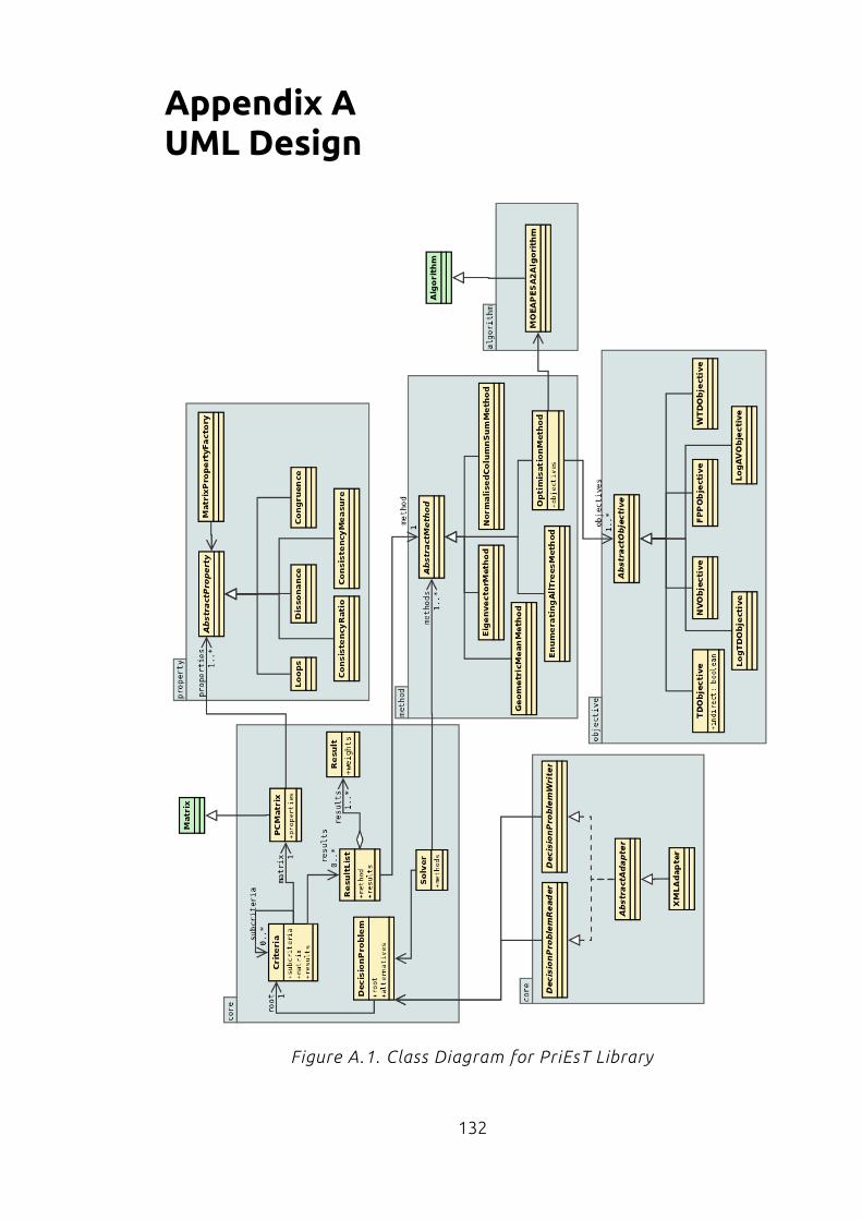
Appendix AUML Design
Figure A.1. Class Diagram for PriEsT Library
132

Figure A.2. Class Diagram for Sensitivity Analysis
133

Appendix BUnit Tests
Figure B.1. System testing performed on previous version of PriEsT
(Siraj, 2011)
134

Figure B.2. Unit testing performed on PriEsT
135
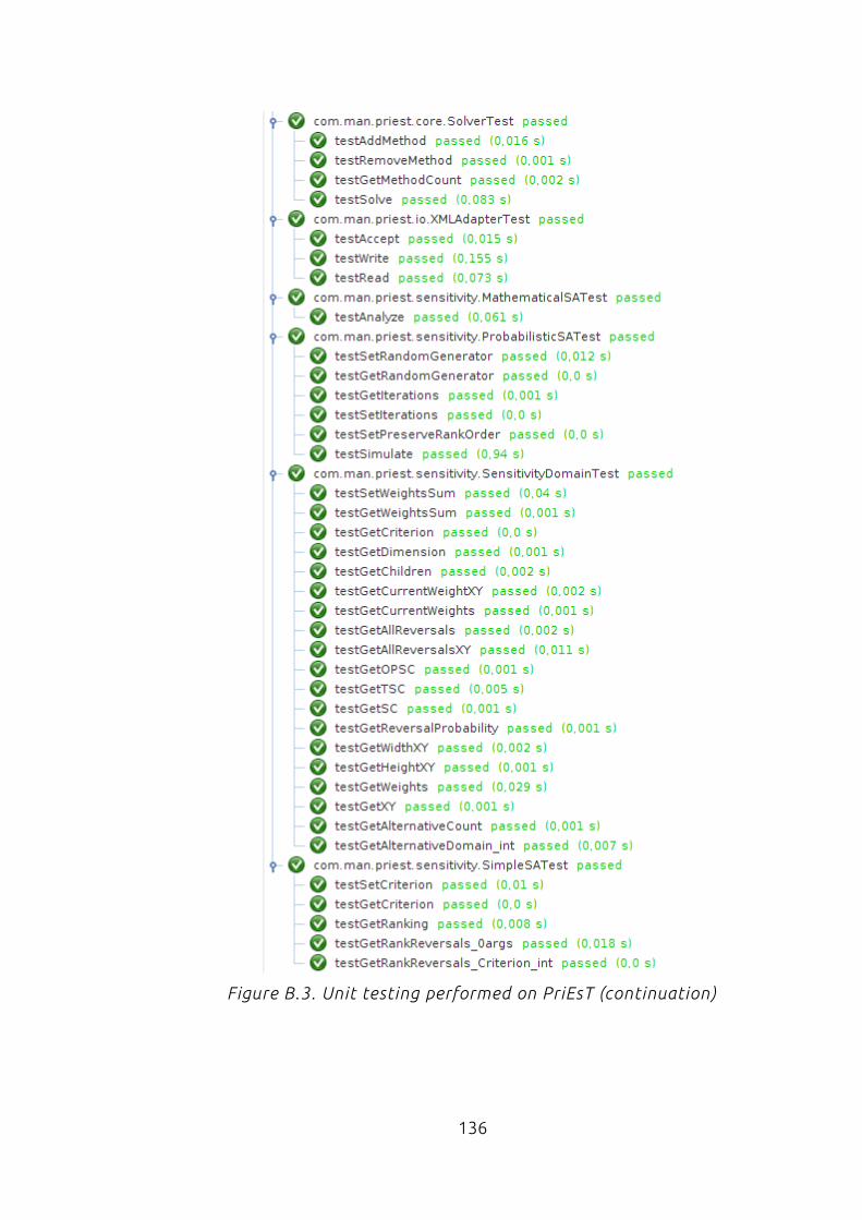
Figure B.3. Unit testing performed on PriEsT (continuation)
136
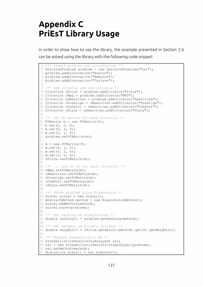
Appendix CPriEsT Library Usage
In order to show how to use the library, the example presented in Section 2.6
can be solved using the library with the following code snippet:
1 /** Create problem and alternatives */ 2 DecisionProblem problem = new DecisionProblem("Car"); 3 problem.addAlternative("Avalon"); 4 problem.addAlternative("Babylon"); 5 problem.addAlternative("Carryon"); 6 7 /** Add criteria and subcriteria */ 8 Criterion cPrice = problem.addCriteria("Price"); 9 Criterion cMpg = problem.addCriteria("MPG");10 Criterion cAmenities = problem.addCriteria("Amenities");11 Criterion cPrestige = cAmenities.addCriterion("Prestige");12 Criterion cComfort = cAmenities.addCriterion("Comfort");13 Criterion cStyle = cAmenities.addCriterion("Style");14 15 /** set PC matrix for each criterion */16 PCMatrix m = new PCMatrix(3);17 m.set(0, 1, 6);18 m.set(0, 2, 3);19 m.set(2, 1, 4);20 problem.setPCMatrix(m);21 22 m = new PCMatrix(3);23 m.set(0, 1, 3);24 m.set(0, 2, 6);25 m.set(1, 2, 4);26 cPrice.setPCMatrix(m);27 28 /** ... and so on for each criterion */29 cMpg.setPCMatrix(m);30 cAmenities.setPCMatrix(m);31 cPrestige.setPCMatrix(m);32 cComfort.setPCMatrix(m);33 cStyle.setPCMatrix(m);34 35 /** Solve problem using Eigenvector */36 Solver solver = new Solver();37 AbstractMethod method = new EigenvectorMethod();38 solver.addMethod(method);39 solver.solve(problem);40 41 /** Get ranking of alternatives */42 double ranking[] = problem.getRanking(method);43 44 /** Get weights of Price's children */45 double weights[] = cPrice.getResult(method).get(0).getWeights();46 47 /** Perform Probabilistic SA */48 ProbabilisticSensitivityAnalyzer sa1;49 sa1 = new ProbabilisticSensitivityAnalyzer(problem);50 sa1.setMethod(method);51 Statistics stats[] = sa1.simulate();
137
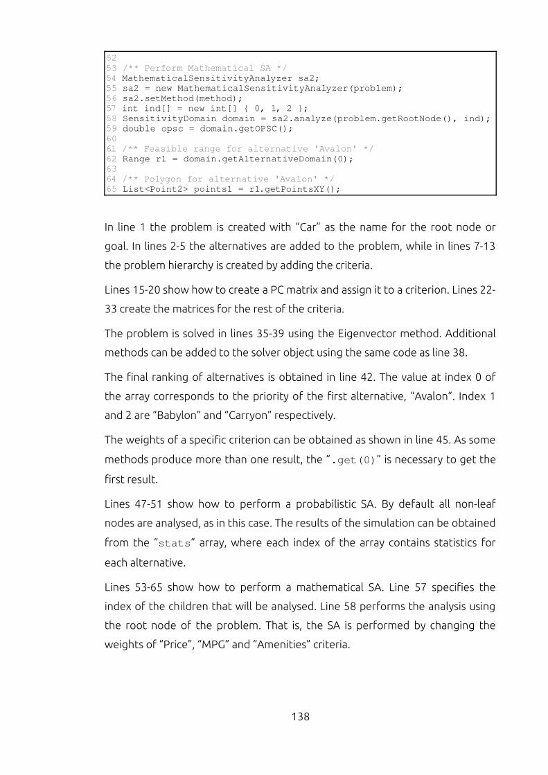
52 53 /** Perform Mathematical SA */ 54 MathematicalSensitivityAnalyzer sa2;55 sa2 = new MathematicalSensitivityAnalyzer(problem);56 sa2.setMethod(method);57 int ind[] = new int[] { 0, 1, 2 };58 SensitivityDomain domain = sa2.analyze(problem.getRootNode(), ind);59 double opsc = domain.getOPSC();60 61 /** Feasible range for alternative 'Avalon' */ 62 Range r1 = domain.getAlternativeDomain(0);63 64 /** Polygon for alternative 'Avalon' */65 List<Point2> points1 = r1.getPointsXY();
In line 1 the problem is created with “Car” as the name for the root node or
goal. In lines 2-5 the alternatives are added to the problem, while in lines 7-13
the problem hierarchy is created by adding the criteria.
Lines 15-20 show how to create a PC matrix and assign it to a criterion. Lines 22-
33 create the matrices for the rest of the criteria.
The problem is solved in lines 35-39 using the Eigenvector method. Additional
methods can be added to the solver object using the same code as line 38.
The final ranking of alternatives is obtained in line 42. The value at index 0 of
the array corresponds to the priority of the first alternative, “Avalon”. Index 1
and 2 are “Babylon” and “Carryon” respectively.
The weights of a specific criterion can be obtained as shown in line 45. As some
methods produce more than one result, the “.get(0)” is necessary to get the
first result.
Lines 47-51 show how to perform a probabilistic SA. By default all non-leaf
nodes are analysed, as in this case. The results of the simulation can be obtained
from the “stats” array, where each index of the array contains statistics for
each alternative.
Lines 53-65 show how to perform a mathematical SA. Line 57 specifies the
index of the children that will be analysed. Line 58 performs the analysis using
the root node of the problem. That is, the SA is performed by changing the
weights of “Price”, “MPG” and “Amenities” criteria.
138

Appendix DApplication Screen-shots
Figure D.1. PriEsT running on Ubuntu Linux
139
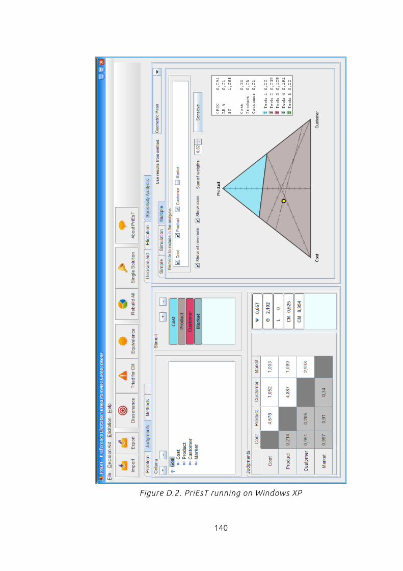
Figure D.2. PriEsT running on Windows XP
140
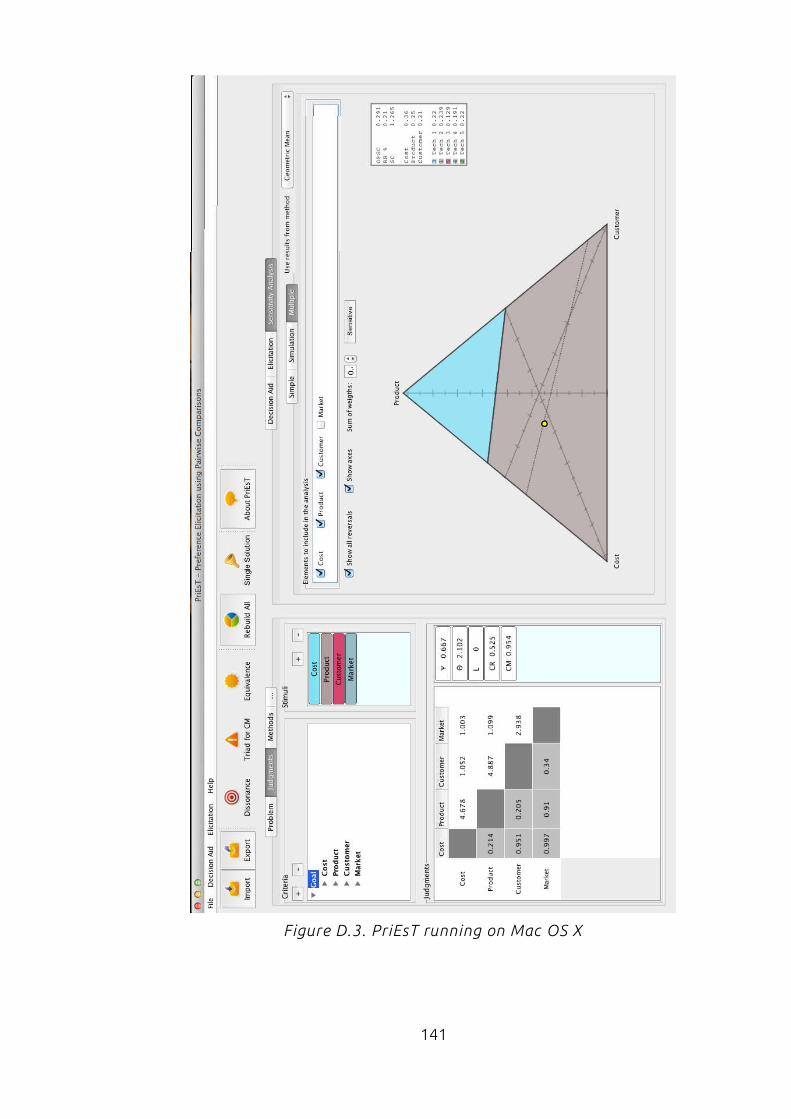
Figure D.3. PriEsT running on Mac OS X
141

Figure D.4. PriEsT Mobile running on Nokia 5800 - J2ME (left) and
Samsung Galaxy S2 - Android (right)
142
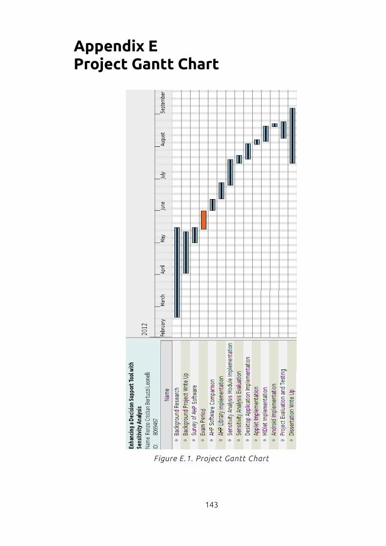
Appendix EProject Gantt Chart
Figure E.1. Project Gantt Chart
143