Embed Size (px)
Citation preview
Enhancements to ConnDOT’s
Pavement Friction Testing Program
Prepared by:
John W. Henault, P.E.
April 2011
Research Project: SPR-2243
Final Report
Report No. CT-2243-F-10-4
Connecticut Department of Transportation
Bureau of Engineering and Construction
Office of Research and Materials
Ravi V. Chandran, P.E.
Division Chief, Research and Materials
ii
DISCLAIMER
The contents of this report reflect the views of the
authors who are responsible for the facts and accuracy of the
data presented herein. The contents do not necessarily reflect
the official views or policies of the Connecticut Department of
Transportation or the Federal Highway Administration. The
report does not constitute a standard, specification or
regulation.
iii
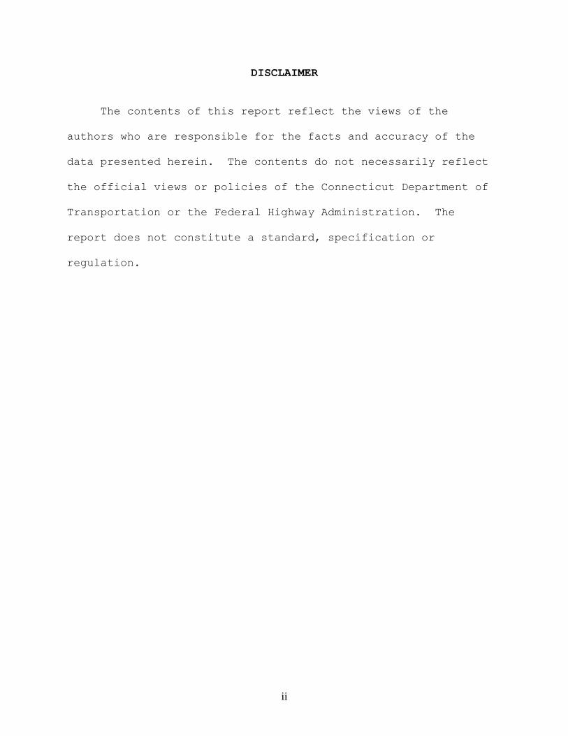
Technical Report Documentation Page
Form DOT F 1700.7 (8-72) Reproduction of completed page authorized
1.Report No.
CT-2243-F-10-4
2. Government Accession No. 3. Recipients Catalog No.
4.
Title and Subtitle
Enhancements to ConnDOT’s Pavement Friction
Testing Program – Final Report
5. Report Date
March 2011
6. Performing Organization Code
SPR-2243
7. Author(s)
John W. Henault
8. Performing Organization Report
No.
CT-2243-F-10-4
9. Performing Organization Name and Address
Connecticut Department of Transportation
Division of Research
280 West Street
Rocky Hill, CT 06067-3502
10. Work Unit No. (TRIS)
11. Contract or Grant No.
CT Study No. SPR-2243
13. Type of Report and Period
Covered
Final Report
2004-2010
12. Sponsoring Agency Name and Address
Connecticut Department of Transportation
2800 Berlin Turnpike
Newington, CT 06131-7546 14. Sponsoring Agency Code
SPR-2243
15. Supplementary Notes
Prepared in cooperation with the U.S. Department of Transportation, Federal
Highway Administration.
16. Abstract
This report documents the work performed and results obtained for research
conducted to enhance ConnDOT’s pavement friction testing program. The program was
enhanced with the purchase in 2005 of a new Dynatest 1295 Pavement Friction Tester.
Upgrades from the previous tester included the addition of a high-speed laser to
measure pavement macrotexture, and a global positioning system to track coordinates.
A Circular Texture Meter was purchased in 2006 to compare to the high-speed laser.
In 2007, the new friction tester was upgraded to a dual-sided system, enabling
testing in either wheelpath. Speed gradients for various ConnDOT pavement surfaces
were determined, the macrotexture of asphalt pavement designs used in Connecticut
were characterized, the use of the International Friction Index was evaluated, and
the effects of roadway geometry on friction measurements were studied. Deliverables
include new and upgraded equipment, recommendations, tentative guidelines for
evaluating friction at high wet accident sites in Connecticut, a procedure for
handling friction test requests, and a draft policy statement.
17. Key Words
Pavement Friction Testing, Skid Testing,
Connecticut Department of Transportation,
ConnDOT, Locked-Wheel Friction Tester
18. Distribution Statement
No restrictions. Hard copy of this document is
available through the National Technical
Information Service, Springfield, VA 22161. The
report is available on-line from the National
Transportation Library at http://ntl.bts.gov
19. Security Classif. (Of this
report)
Unclassified
20. Security Classif.(Of this
page)
Unclassified
21. No. of
Pages
89
20.
Price
iv
ACKNOWLEDGEMENTS
The author gratefully acknowledges the support of the
Connecticut Department of Transportation (ConnDOT) and the U.S.
Federal Highway Administration. The author thanks Messrs.
Donald Larsen and Eric Feldblum for initiating this project and
for providing data/information collected in an organized manner
upon their transferring to other Department positions. A
special thank you is extended to Mr. Jeffery Scully for his
contribution to this study and to ConnDOT’s Friction Testing and
Safety Evaluation Services program. Messrs. Drew Coleman and
James Moffett are thanked for providing video production
services during presentations related to this study. Ms. Susan
Hulme is acknowledged for providing administrative assistance
and Mr. James Sime for providing project oversight. Finally,
the following individuals are acknowledged and thanked for their
contributions: Ms. Jessica Bliven, Mr. Lester King, Robert
Kasica, Sarah Rakowski, and Frank Romano.
v
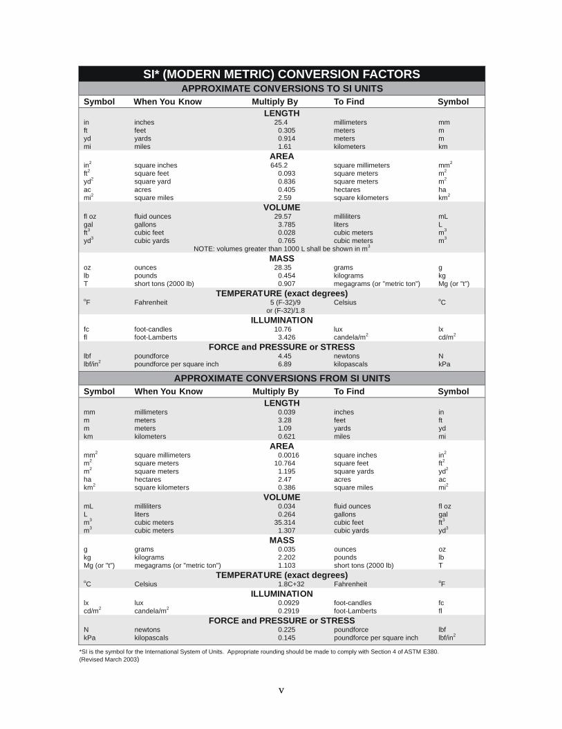
SI* (MODERN METRIC) CONVERSION FACTORS APPROXIMATE CONVERSIONS TO SI UNITS
Symbol When You Know Multiply By To Find Symbol
LENGTH in inches 25.4 millimeters mm
ft feet 0.305 meters m
yd yards 0.914 meters m mi miles 1.61 kilometers km
AREA in
2square inches 645.2 square millimeters mm
2
ft2
square feet 0.093 square meters m2
yd2
square yard 0.836 square meters m2
ac acres 0.405 hectares ha
mi2
square miles 2.59 square kilometers km2
VOLUME fl oz fluid ounces 29.57 milliliters mL
gal gallons 3.785 liters L ft
3 cubic feet 0.028 cubic meters m
3
yd3
cubic yards 0.765 cubic meters m3
NOTE: volumes greater than 1000 L shall be shown in m3
MASS oz ounces 28.35 grams g
lb pounds 0.454 kilograms kg
T short tons (2000 lb) 0.907 megagrams (or "metric ton") Mg (or "t")
TEMPERATURE (exact degrees) oF Fahrenheit 5 (F-32)/9 Celsius
oC
or (F-32)/1.8
ILLUMINATION fc foot-candles 10.76 lux lx fl foot-Lamberts 3.426 candela/m
2 cd/m
2
FORCE and PRESSURE or STRESS lbf poundforce 4.45 newtons N
lbf/in2
poundforce per square inch 6.89 kilopascals kPa
APPROXIMATE CONVERSIONS FROM SI UNITS
Symbol When You Know Multiply By To Find Symbol
LENGTHmm millimeters 0.039 inches in
m meters 3.28 feet ft
m meters 1.09 yards yd
km kilometers 0.621 miles mi
AREA mm
2 square millimeters 0.0016 square inches in
2
m2 square meters 10.764 square feet ft
2
m2 square meters 1.195 square yards yd
2
ha hectares 2.47 acres ac
km2
square kilometers 0.386 square miles mi2
VOLUME mL milliliters 0.034 fluid ounces fl oz
L liters 0.264 gallons gal
m3
cubic meters 35.314 cubic feet ft3
m3
cubic meters 1.307 cubic yards yd3
MASS g grams 0.035 ounces oz
kg kilograms 2.202 pounds lbMg (or "t") megagrams (or "metric ton") 1.103 short tons (2000 lb) T
TEMPERATURE (exact degrees) oC Celsius 1.8C+32 Fahrenheit
oF
ILLUMINATION lx lux 0.0929 foot-candles fc
cd/m2
candela/m2
0.2919 foot-Lamberts fl
FORCE and PRESSURE or STRESS N newtons 0.225 poundforce lbf
kPa kilopascals 0.145 poundforce per square inch lbf/in2
*SI is the symbol for th International System of Units. Appropriate rounding should be made to comply with Section 4 of ASTM E380. e
(Revised March 2003)
vi
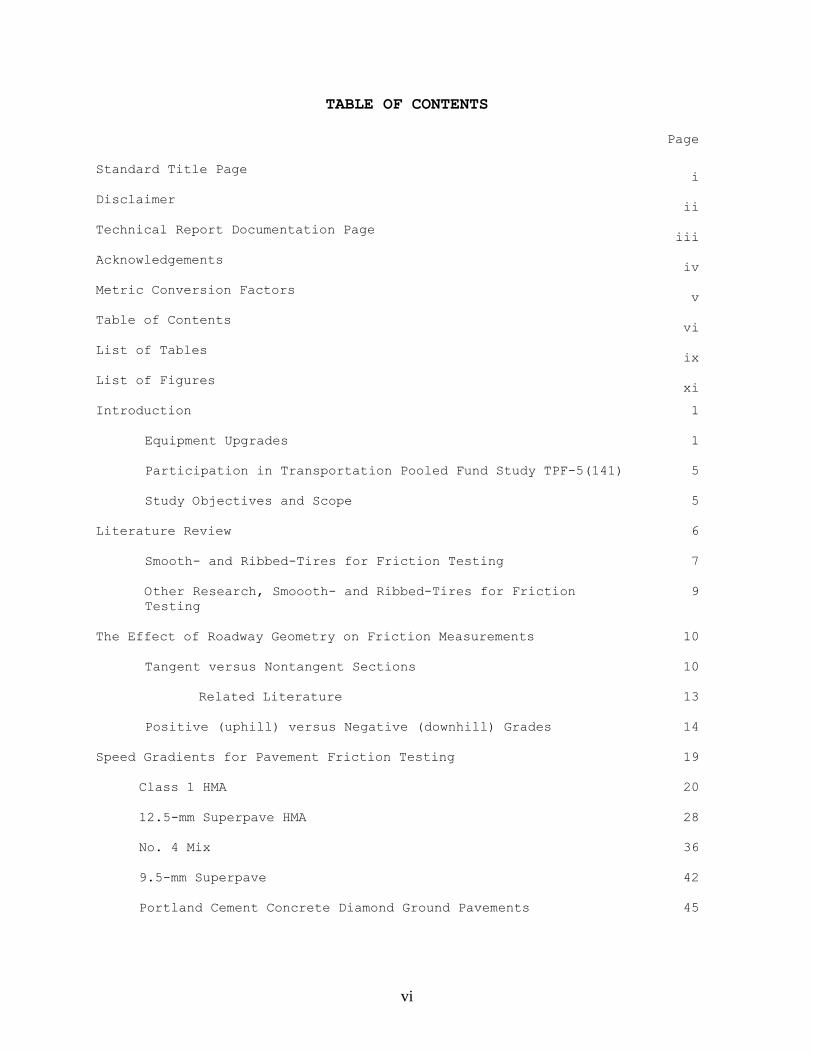
TABLE OF CONTENTS
Page
Standard Title Page
i
Disclaimer
ii
Technical Report Documentation Page
iii
Acknowledgements
iv
Metric Conversion Factors
v
Table of Contents
vi
List of Tables
ix
List of Figures
xi
Introduction 1
Equipment Upgrades
1
Participation in Transportation Pooled Fund Study TPF-5(141)
5
Study Objectives and Scope 5
Literature Review
6
Smooth- and Ribbed-Tires for Friction Testing
7
Other Research, Smoooth- and Ribbed-Tires for Friction
Testing
9
The Effect of Roadway Geometry on Friction Measurements
10
Tangent versus Nontangent Sections 10
Related Literature
13
Positive (uphill) versus Negative (downhill) Grades 14
Speed Gradients for Pavement Friction Testing 19
Class 1 HMA 20
12.5-mm Superpave HMA 28
No. 4 Mix 36
9.5-mm Superpave 42
Portland Cement Concrete Diamond Ground Pavements 45
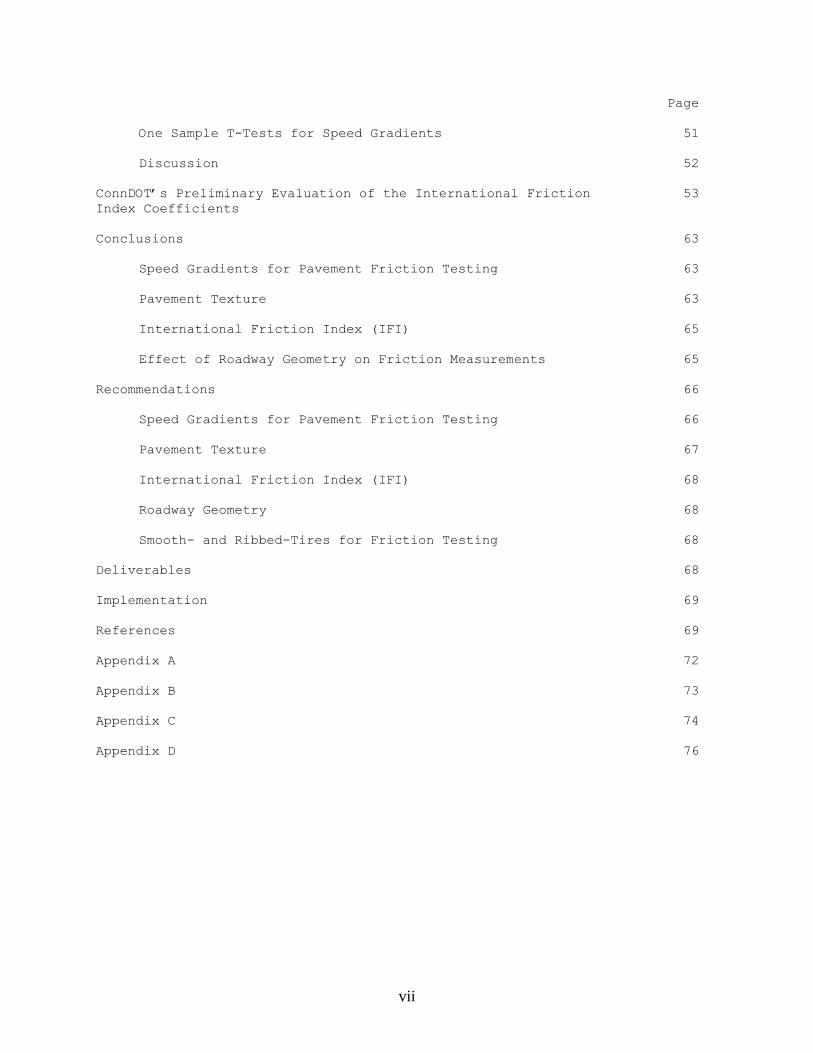
vii
Page
One Sample T-Tests for Speed Gradients 51
Discussion
52
ConnDOT’s Preliminary Evaluation of the International Friction
Index Coefficients
53
Conclusions 63
Speed Gradients for Pavement Friction Testing 63
Pavement Texture 63
International Friction Index (IFI) 65
Effect of Roadway Geometry on Friction Measurements 65
Recommendations 66
Speed Gradients for Pavement Friction Testing 66
Pavement Texture 67
International Friction Index (IFI) 68
Roadway Geometry 68
Smooth- and Ribbed-Tires for Friction Testing 68
Deliverables 68
Implementation 69
References 69
Appendix A 72
Appendix B 73
Appendix C 74
Appendix D 76
viii
LIST OF TABLES Page
TABLE 1 Friction Test Values Measured on 28° Right Hand Horizontal
Curve
11
TABLE 2 Friction Test Values Measured on 24° Right Hand Horizontal
Curve
11
TABLE 3 Friction Test Values Measured on Straight Tangent, Gate 1
12
TABLE 4 Friction Test Values Measured on Straight Tangent, Gate 2
12
TABLE 5 Friction Test Values Measured on Straight Tangent, Gate 3
12
TABLE 6 Route 66 WB, Approximate Grade = 5% to 7.0% (Uphill)
15
TABLE 7 Route 66 EB, Approximate Grade = -5% to -7.0% (Downhill)
16
TABLE 8 Route 66 EB, Approximate Grade = 6.5% to 7.0% (Uphill)
17
TABLE 9 Route 66 WB, Approximate Grade = -6.5% to -7.0% (Downhill) 18
TABLE 10 Class 1 HMA Speed Gradient Slopes and R2 Values by Milepost
10
TABLE 11 Class 1 HMA Speed Gradient Slopes and R2 Values by Site
21
TABLE 12 Speed Gradients and R2 values by milepost on 12.5-mm
Superpave pavements.
29
TABLE 13 Speed Gradients and R2 values by site on 12.5-mm Superpave
pavements.
29
TABLE 14 No. 4 Mix Speed Gradient Slopes and R2 Values by Milepost 37
TABLE 15 No. 4 Mix HMA Speed Gradient Slopes and R2 Values by Site
37
TABLE 16 9.5-mm Superpave HMA Speed Gradient Slopes and R2 Values by
Site
43
TABLE 17 PCC Diamond Ground Pavement Speed Gradient Slopes and R2
Values by Milepost
46
TABLE 18 PCC Diamond Ground Pavement Speed Gradient Slopes and R2
Values by Site
46
TABLE 19 One Sample Statistics for Speed Gradient
52
TABLE 20 One Sample Tests for Speed Gradients
52
TABLE 21 International Friction Index Parameters (Sp and F60)
Calculated with ConnDOT Measurements for Smart Road Sections
56
ix
Page
TABLE 22 IFI Parameters Measured in Front of ConnDOT Central Lab,
Starting at Lab Driveway Heading WB, SuperPave 12.5 mm
September 17, 2007
59
TABLE 23 IFI Parameters Measured in Front of ConnDOT Central Lab,
Starting at Lab Driveway Heading WB, SuperPave 12.5 mm
June 4, 2008
59
TABLE 24 IFI Parameters Measured in Front of ConnDOT Central Lab,
Starting at Lab Driveway Heading WB, SuperPave 12.5 mm July 2, 2008
60
TABLE 25 IFI Parameters Measured in Front of ConnDOT Central Lab,
Starting at Lab Driveway Heading WB, 12.5-mm Superpave, October 14,
2008
60
TABLE 26 International Friction Index Summary in Front of ConnDOT
Central Lab, Starting at Lab Driveway Heading WB, 12.5-mm Superpave
61
TABLE 27 Descriptive Statistics for IFI Parameters Calculated for
Tests Performed at or near 50 mph
62
TABLE 28 Descriptive Statistics for IFI Parameters Calculated for
Tests Performed at or near 30 mph
62
TABLE A-1 Tentative Guidelines for Evaluating Friction at High Wet
Accident Sites in Connecticut
72

x
LIST OF FIGURES
Page
FIGURE 1 Dynatest 1295 Pavement Friction Tester.
2
FIGURE 2 Housing for High-Speed Selcom
Optocator/SLS5000 Laser Sensor.
2
FIGURE 3 Trimble Model AgGPS 33300-00 Global
Positioning System.
3
FIGURE 4 Nippo Sangyo Co., Ltd. Circular Track Meter
purchased in 2006.
3
FIGURE 5 Inside the cab of the Dynatest 1295 Pavement
Friction Tester purchased in 2005.
4
FIGURE 6 Ohio State Water Nozzle used to wet pavement
in front of test tires.
5
FIGURE 7 Simple Error Bar Defined at 98% Confidence
Interval for Mean FN40R Values.
13
FIGURE 8 98% Confidence Intervals for FN40R values.
19
FIGURE 9 Speed gradients at individual mileposts for
Route 3 SB Class 1 pavement in Cromwell.
22
FIGURE 10 Speed gradients combined for Route 3 SB
Class 1 pavement in Cromwell.
22
FIGURE 11 Speed gradients at individual mileposts for
Route 3 NB Class 1 pavement in Cromwell.
23
FIGURE 12 Speed gradients combined for Route 3 NB
Class 1 pavement in Cromwell.
23
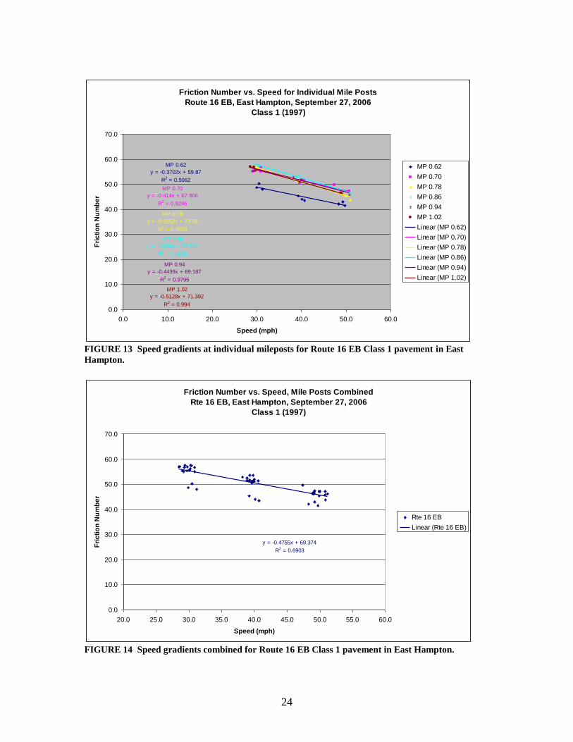
FIGURE 13 Speed gradients at individual mileposts for
Route 16 EB Class 1 pavement in East Hampton.
24
FIGURE 14 Speed gradients combined for Route 16 EB
Class 1 pavement in East Hampton.
24
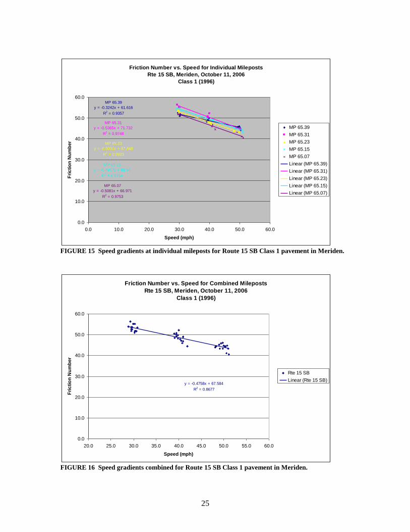
FIGURE 15 Speed gradients at individual mileposts for
Route 15 SB Class 1 pavement in Meriden.
25
xi
LIST OF FIGURES (Continued)
Page
FIGURE 16 Speed gradients combined for Route 15 SB
Class 1 pavement in Meriden.
25
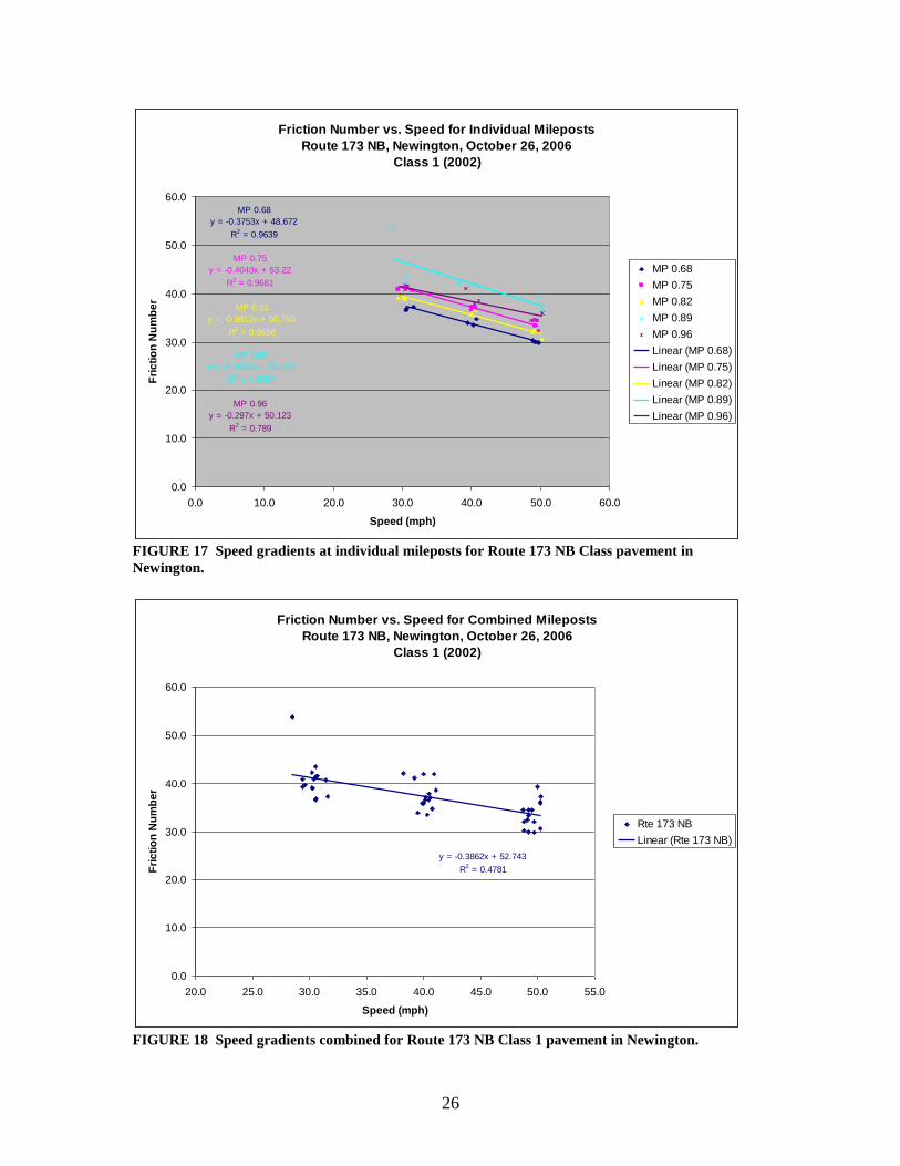
FIGURE 17 Speed gradients at individual mileposts for
Route 173 NB Class pavement in Newington.
26
FIGURE 18 Speed gradients combined for Route 173 NB
Class 1 pavement in Newington.
26
FIGURE 19 98% Confidence intervals for speed gradients
for Class 1 pavements.
27
FIGURE 20 Speed gradients at individual mileposts for
Route 411 EB SP 12.5-mm pavement in Rocky Hill.
30
FIGURE 21 Speed gradients combined for Route 411 EB SP
12.5-mm pavement in Newington.
30
FIGURE 22 Speed gradients at individual mileposts for
Route 411 WB SP 12.5-mm pavement in Rocky Hill.
31
FIGURE 23 Speed gradients combined for Route 411 WB SP
12.5-mm pavement in Rocky Hill.
31
FIGURE 24 Speed gradients at individual mileposts for
Route 15 NB SP 12.5-mm pavement in Berlin.
32
FIGURE 25 Speed gradients combined for Route 15 NB SP
12.5-mm pavement in Berlin.
32
FIGURE 26 Speed gradients at individual mileposts for
Route 94 EB SP 12.5-mm pavement in Hebron.
33
FIGURE 27 Speed gradients combined for Route 94 EB SP
12.5-mm pavement in Hebron.
33
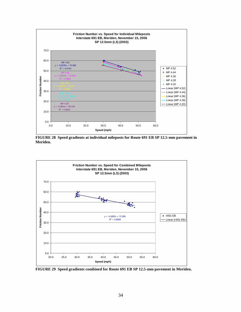
FIGURE 28 Speed gradients at individual mileposts for
Route 691 EB SP 12.5-mm pavement in Meriden.
34
FIGURE 29 Speed gradients combined for Route 691 EB SP
12.5-mm pavement in Meriden.
34
xii
LIST OF FIGURES (Continued)
Page
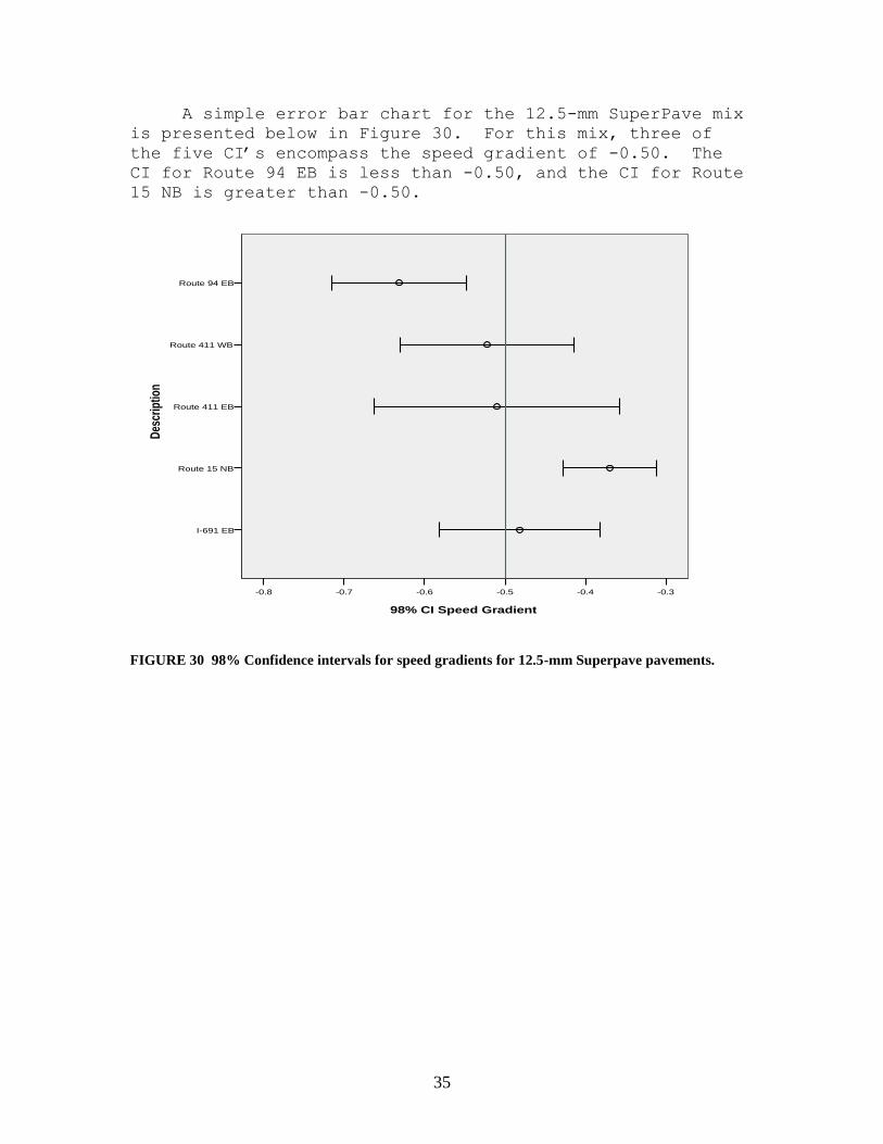
FIGURE 30 98% Confidence intervals for speed gradients
for 12.5-mm Superpave pavements.
35
FIGURE 31 Speed gradients at individual mileposts for
Route 9 NB SP #4 pavement in Haddam.
38
FIGURE 32 Speed gradients combined for Route 9 NB SP
#4 pavement in Haddam.
38
Figure 33 Speed gradients at individual mileposts for
Route 9 SB SP #4 pavement in Chester.
39
FIGURE 34 Speed gradients combined for Route 9 SB SP
#4 pavement in Chester.
39
FIGURE 35 Speed gradients at individual mileposts for
Route 2 EB SP #4 pavement in Colchester.
40
FIGURE 36 Speed gradients combined for Route 2 EB SP
#4 pavement in Colchester.
40
FIGURE 37 Speed gradients at individual mileposts for
Route 2 WB SP #4 pavement in Colchester.
41
FIGURE 38 Speed gradients combined for Route 2 WB SP
#4 pavement in Colchester.
41
FIGURE 39 98% Confidence intervals for speed gradients
for SuperPave No. 4 pavements.
42
FIGURE 40 Speed gradients at individual mileposts for
I-91 NB SP 9.5-mm pavement in North Haven.
43
FIGURE 41 Speed gradients combined for I-91 NB 9.5-mm
SP pavement in North Haven.
44
FIGURE 42 98% Confidence interval for speed gradient
for 9.5-mm SuperPave pavement on I-91 NB in North
Haven.
45
FIGURE 43 Speed gradients at individual mileposts for
I-691 EB Diamond Ground PCC pavement in Cheshire.
47
xiii
LIST OF FIGURES (Continued)
Page
FIGURE 44 Speed gradients combined for I-691 NB
Diamond Ground PCC pavement in Cheshire.
47
FIGURE 45 Speed gradients at individual mileposts for
I-691 WB Diamond Ground PCC pavement in Cheshire.
48
FIGURE 46 Speed gradients combined for I-691 WB
Diamond Ground PCC pavement in Cheshire.
48
FIGURE 47 Speed gradients at individual mileposts for
Route 9 SB Diamond Ground PCC pavement in New Britain.
49
FIGURE 48 Speed gradients combined for Route 9 SB
Diamond Ground PCC pavement in New Britain.
49
FIGURE 49 Speed gradients at individual mileposts for
Route 9 NB Diamond Ground PCC pavement in New Britain.
50
FIGURE 50 Speed gradients combined for Route 9 NB
Diamond Ground PCC pavement in New Britain.
50
FIGURE 51 98% Confidence interval for speed gradients
for PCC Diamond Ground pavement.
51
FIGURE 52 F60 Values Calculated from High-Speed Laser
MPDs versus F60 Values Calculated with CTMeter MPDs
57
FIGURE 53 Sp Values Calculated from High-Speed Laser
MPDs versus F60 Values Calculated with CTMeter MPDs.
57
1
INTRODUCTION
This project was proposed for inclusion in the
Connecticut State Planning and Research (SP&R) Work Program
in May 2004 in order to address the Connecticut Department
of Transportation’s (ConnDOT’s) need to upgrade its
friction testing equipment (1). At that time, a fifteen-
year-old 1989 KJ Law Model 1290 pavement friction tester,
with a retrofitted trailer (2000) was being used to perform
pavement friction tests. Historically, ConnDOT pavement
friction testers were replaced on a ten-year schedule.
This is the third and final report published for this
project. The first report (CT-2243-1-10-1) titled
“Historical Overview of Pavement Friction Testing in
Connecticut” provides a concise historical reference for
current and future employees (2). It fits into the
succession planning that should take place within a state
highway agency prior to retirements and changes in employee
responsibilities.
The second report (CT-2243-2-10-3) titled
“Characterizing the Macrotexture of Asphalt Pavement
Designs in Connecticut” presents results of ConnDOT’s
efforts to establish targets for pavement texture depth on
high-speed facilities by characterizing the macrotexture of
a few different ConnDOT hot-mix asphalt (HMA) pavement
mixes (3).
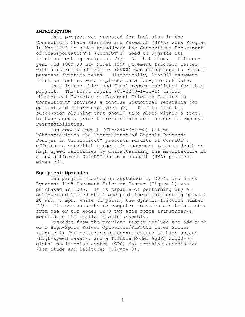
Equipment Upgrades
The project started on September 1, 2004, and a new
Dynatest 1295 Pavement Friction Tester (Figure 1) was
purchased in 2005. It is capable of performing dry or
self-wetted locked wheel and peak incipient testing between
20 and 70 mph, while computing the dynamic friction number
(4). It uses an on-board computer to calculate this number
from one or two Model 1270 two-axis force transducer(s)
mounted to the trailer’s axle assembly.
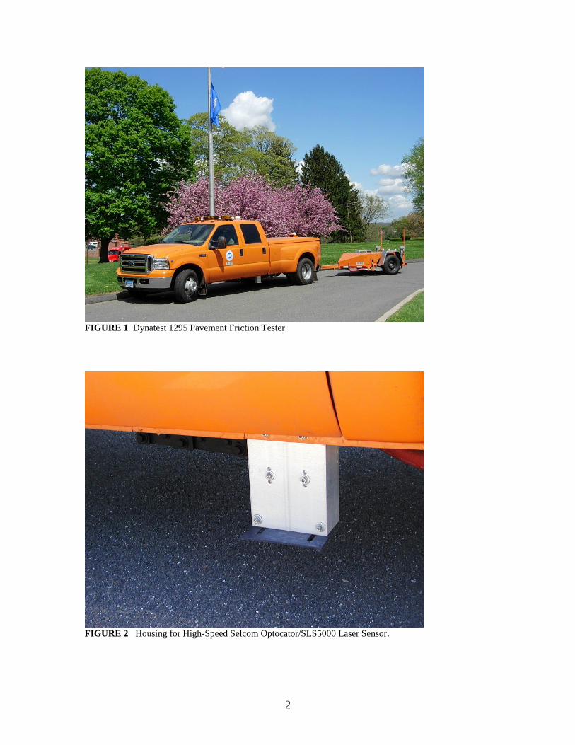
Upgrades from the previous tester include the addition
of a High-Speed Selcom Optocator/SLS5000 Laser Sensor
(Figure 2) for measuring pavement texture at high speeds
(high-speed laser), and a Trimble Model AgGPS 33300-00
global positioning system (GPS) for tracking coordinates
(longitude and latitude) (Figure 3).
2
FIGURE 1 Dynatest 1295 Pavement Friction Tester.
FIGURE 2 Housing for High-Speed Selcom Optocator/SLS5000 Laser Sensor.
3
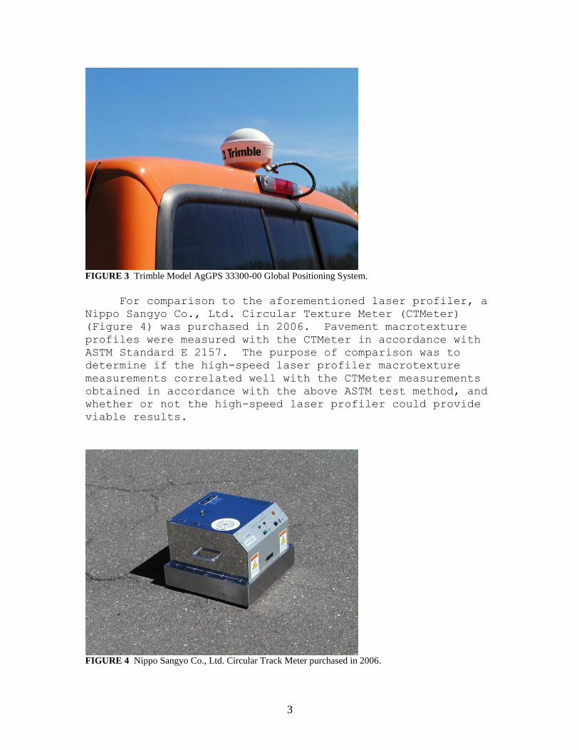
FIGURE 3 Trimble Model AgGPS 33300-00 Global Positioning System.
For comparison to the aforementioned laser profiler, a
Nippo Sangyo Co., Ltd. Circular Texture Meter (CTMeter)
(Figure 4) was purchased in 2006. Pavement macrotexture
profiles were measured with the CTMeter in accordance with
ASTM Standard E 2157. The purpose of comparison was to
determine if the high-speed laser profiler macrotexture
measurements correlated well with the CTMeter measurements
obtained in accordance with the above ASTM test method, and
whether or not the high-speed laser profiler could provide
viable results.
FIGURE 4 Nippo Sangyo Co., Ltd. Circular Track Meter purchased in 2006.
4
In August 2007, the Dynatest 1295 Pavement Friction
Tester was upgraded from a single-sided to a dual-sided
system. This entails that two Model 1270 two-axis force
transducers are now mounted to the axle assembly of the
trailer: one on the left side (driver’s side) and one on
the right side (passenger’s side). The single-sided system
could only measure friction in the driver’s side wheel
path. The dual-sided system is capable of measuring
pavement friction in either wheel path. This provides the
operator with several choices. Pavement friction tests can
be alternated between the left and right wheels, or tests
can be performed exclusively with either the left or right
wheel; however, tests cannot be performed with the left and
right wheels simultaneously. A ribbed tire can be mounted
on one side, and a smooth tire on the other, which allows
ribbed and smooth tire tests to be performed without having
to change tires. Alternatively, the same tire (ribbed or
smooth) can be mounted on both wheels, allowing either
ribbed or smooth tire friction measurements in both wheel
paths.
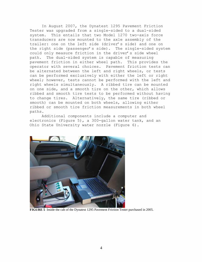
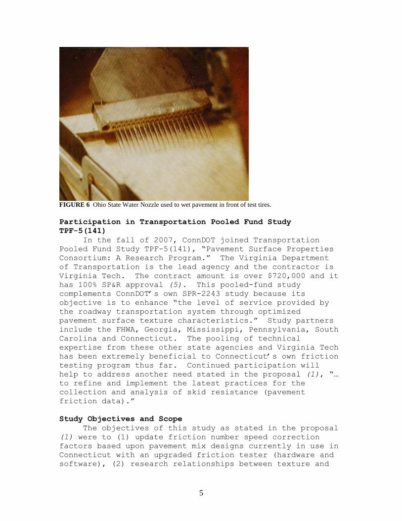
Additional components include a computer and
electronics (Figure 5), a 300-gallon water tank, and an
Ohio State University water nozzle (Figure 6).
FIGURE 5 Inside the cab of the Dynatest 1295 Pavement Friction Tester purchased in 2005.
5
FIGURE 6 Ohio State Water Nozzle used to wet pavement in front of test tires.
Participation in Transportation Pooled Fund Study
TPF-5(141)
In the fall of 2007, ConnDOT joined Transportation
Pooled Fund Study TPF-5(141), “Pavement Surface Properties
Consortium: A Research Program.” The Virginia Department
of Transportation is the lead agency and the contractor is
Virginia Tech. The contract amount is over $720,000 and it
has 100% SP&R approval (5). This pooled-fund study
complements ConnDOT’s own SPR-2243 study because its
objective is to enhance “the level of service provided by
the roadway transportation system through optimized
pavement surface texture characteristics.” Study partners
include the FHWA, Georgia, Mississippi, Pennsylvania, South
Carolina and Connecticut. The pooling of technical
expertise from these other state agencies and Virginia Tech
has been extremely beneficial to Connecticut’s own friction
testing program thus far. Continued participation will
help to address another need stated in the proposal (1), “…
to refine and implement the latest practices for the
collection and analysis of skid resistance (pavement
friction data).”
Study Objectives and Scope
The objectives of this study as stated in the proposal
(1) were to (1) update friction number speed correction
factors based upon pavement mix designs currently in use in
Connecticut with an upgraded friction tester (hardware and
software), (2) research relationships between texture and
6
friction, (3) evaluate the potential use of the
International Friction Index (IFI) in Connecticut, and, (4)
implement the appropriate latest technology and procedures
for pavement friction data request, collection and
processing.
As discussed above, a CTMeter was purchased in 2006 in
order to compare texture values measured with the CTMeter
to the high-speed laser profiler. Accordingly, the scope
of this report also includes a presentation of the laser
profiler versus CTMeter macrotexture measurement
comparisons performed at the Virginia Smart Road facility,
as part of TPF-5(141). CTMeter measurements were taken
with the ConnDOT instrument and also with Virginia Tech’s
CTMeter on twelve different pavement designs. This paper
presents measurements taken with ConnDOT’s CTMeter. Three
CTMeter measurements were taken and averaged for each
pavement design. These pavement designs encompassed a wide
range of textures, from fine to coarse. The goal of these
comparisons was to provide some validation of the laser
profiler macrotexture measurements as they compared to the
CTMeter measurements obtained in accordance with ASTM E
2157.
In observance of a Federal Highway Administration
(FHWA) Technical Advisory entitled Surface Texture for
Asphalt and Concrete Pavements (6), another objective
evolved to begin to establish targets for pavement texture
depth on high-speed facilities by characterizing the
macrotexture of different ConnDOT hot-mix asphalt (HMA)
pavement mixes. The nominal maximum aggregate size for
these designs ranged from 4.75-mm to 12.5-mm. Part of this
effort to characterize pavement macrotexture is to begin
taking the first steps in establishing texture depth
targets for new and in-service pavement surfaces in
Connecticut. The advisory states “providing adequate
texture depth has been shown to improve pavement friction
test results at high speeds and reduce crash rates on high
speed facilities.” The advisory suggests these targets be
established by owner-agencies based upon project specific
factors, such as roadway geometry (6). This effort was
largely presented in Report No. CT-2243-2-10-3 (3), but is
summarized in the conclusions of this final report as well.
LITERATURE REVIEW
A historical overview of pavement friction testing in
Connecticut is presented in Report CT-2243-1-10-1 (2).
This effort will not be duplicated in this final report,
but a literature review is presented below.
7
The Guide for Pavement Friction (7) defines pavement
friction as “…the force that resists the relative motion
between a vehicle tire and a pavement surface.” They
identified two modes of operation for the longitudinal
dynamic friction process: free-rolling and constant-braked.
In the free-rolling mode, something called the slip speed
is zero. The slip speed is defined as “the relative speed
between the tire circumference and the pavement”. In the
constant-braked mode, the slip speed approaches the vehicle
speed.
Slip is more commonly referred to in terms of its
percent ratio to the vehicle velocity. “A locked-wheel
state is often referred to as a 100 percent slip ratio and
the free-rolling state is a zero percent slip ratio.” The
peak friction that is reached during braking typically
occurs between 10 and 20 percent slip (7). Most new cars
today are equipped with anti-lock brakes, which pump the
brakes repeatedly in order to operate at or near this peak
value. Pavement friction testers experience the entire
cycle during the locked-wheel test, from free rolling to
100 percent slip. The reported friction number is an
average of readings measured during 100 percent slip.
Modern testers, such as the Dynatest Model 1295, also
calculate the peak friction that occurs prior to lockup.
Smooth- and Ribbed-Tires for Friction Testing
Either an AASHTO M 261, “Standard Tire for Pavement
Frictional-Property Tests” or an AASHTO M 286, “Smooth-
Tread Standard Tire for Special-Purpose Pavement
Frictional-Property Tests” can be used for conducting the
tests. While the AASHTO nomenclature for the smooth tire
suggests a different status for the smooth tire by saying
it’s for “special-purpose” tests, the ASTM counterpart
standards give both tires equal status (8): ASTM E 524,
“Standard Smooth Tire for Pavement Skid-Resistance Tests”
and ASTM E 501, “Standard Rib Tire for Pavement Skid-
Resistance Tests.”
The ribbed tire has been the standard test tire used
in Connecticut for friction testing since the inception of
the friction testing program in Connecticut in 1970.
Initially, it was used because it was considered the
standard test tire by ASTM. Early on, ASTM chose the
ribbed tire as the standard because it was believed that it
was less sensitive to the water flow rate and therefore
results would be more reproducible. The ribbed tire
continued to be used as the standard tire in Connecticut
8
even after the smooth tire was given equal status in 1990.
This was largely due to inertia. ConnDOT engineers were
comfortable with making decisions based upon ribbed tire
friction test values, and historical results were readily
available. The smooth tire was used on occasion upon
request or for research purposes.
In the 1970s, Ganung and Kos (9) performed smooth-tire
testing during a research study to identify and evaluate
wet-weather high-hazard locations in Connecticut. The
study was conducted because they had found during inventory
testing between 1973 and 1974 that measured ribbed-tire
friction values were frequently high in areas showing high
percentages of wet-weather accidents (9). They were
surprised by these experiences, so they decided to perform
smooth-tire friction tests “to determine if these
apparently hydroplaning-prone areas could be delineated by
this means.” Their rationale was that a smooth tire “will
experience dynamic hydroplaning with a much smaller
quantity of water than will the standard ASTM E501 ribbed
test tire.” They felt that the smooth tire would be a
better “indicator of pavement conditions conducive to
hydroplaning in very heavy rain.”
They coupled these smooth-tire measurements with
smooth-tire measurements obtained previously and found that
“…low smooth-tire numbers are quite common throughout the
State, with values ranging from the mid twenties to as low
as three or four.” Counterpart ribbed-tire values did not
always correspond to these low smooth-tire values, as
instances of ribbed-tire values in the fifties were not
unusual. They also found a “good correspondence between
low smooth-tire skid numbers and accident experience”, and
that ribbed tire values did not correspond well to accident
experiences (9). This is significant because the ribbed
tire values did not always correspond with low smooth-tire
values. If low smooth-tire values do in fact correspond to
accident experiences as Ganung and Kos suggested and
ribbed-tire values do not, then the smooth tire should be
the standard test tire – not the ribbed tire.
In their conclusions, Ganung and Kos (9) stated
“Inventory tests on the Merritt Parkway indicated that 95
percent of the wet weather accidents occurred where smooth
tire skid numbers were 15 or lower, and only five percent
took place with values above 15.” They did not find any
accidents that appeared to be related to dynamic
hydroplaning for areas that had smooth-tire friction values
greater than about 25. Perhaps consideration should be
9
given to setting an intervention level for smooth-tire
friction values of less than 15.
Ganung and Kos (9) attempted to relate smooth-tire
friction values at a fixed speed with ribbed-tire speed
gradients, but were unsuccessful. They were also unable
to develop a rigorous association between friction values
and texture depths.
Ultimately, because the majority of the smooth-tire
friction values measured during their study were below 30,
Ganung and Kos (9) recommended that the then existing
friction testing inventory system be expanded to include
smooth-tire testing in order to determine descriptive
statistics.
Other Research, Smooth- and Ribbed-Tires for Friction
Testing
In 1992, Transportation Research Record (TRB) 1348 was
published. This publication included work, sponsored by
the Pennsylvania Department of Transportation, by Henry and
Wambold (10) who wrote a paper titled “Use of Smooth-
Treaded Test Tire in Evaluating Skid Resistance.” They
recommended that both tires be used for project-level
surveys. In circumstances for which only one tire can be
used, they recommended the smooth tire because “it is
sensitive to macro- and microtexture whereas the ribbed
tire responds primarily to the microtexture.”
The Illinois Department of Transportation performed
smooth- and ribbed-tire friction testing during the 1980’s.
An overview of their work is also presented in TRB Record
1348 by Hall et al (11). They presented tentative
guidelines for evaluating friction at high wet-pavement
accident sites in two tables. The first table was for
accident sites before 1987 with ribbed-tire values only,
and the second table was for accident sites after 1987
incorporating both ribbed- and smooth-tire friction values.
For instances where ribbed-tire values were less than or
equal to 30 or smooth-tire values were less than 15, their
tentative guideline was “Friction is probably a factor
contributing to wet-pavement accidents.” When ribbed-tire
values were greater than 30 and smooth-tire values were
between 15 and 25, or ribbed-tire values were between 31
and 35 and smooth-tire values were greater than 25, the
guideline was “Uncertainty exists as to whether pavement
friction is the primary factor.” Finally, for instances
where ribbed-tire values were greater than or equal to 36
and smooth-tire values were greater than 25, their
guideline was “Probably some condition other than pavement
10
friction may be the primary factor causing wet pavement
accidents.”
The Indiana Department of Transportation recently
upgraded their friction testing program and investigated
using the smooth tire. In a 2003 published report titled
“Upgrading the INDOT Pavement Friction Testing Program,”
they recommended the standard smooth tire for network level
pavement friction testing. They also recommended a minimum
smooth-tire friction value of 20 at 40 mph for network
pavement inventory friction testing. They felt that this
requirement would be economically reasonable (12).
Personnel at the National Aeronautics and Space
Administration (NASA) Langley Research Center’s Landing and
Impacts Dynamic Branch provided a summary of their ribbed-
and smooth-tire friction values in TRB Record 1348. Yager
(13) reported that the smooth tire was “more sensitive to
variations in speed, surface texture, and contaminants than
the ASTM E501 rib-tread tire.” He also pointed out that
the smooth tire is not influenced by tire wear.
THE EFFECT OF ROADWAY GEOMETRY ON FRICTION MEASUREMENTS
Tangent versus Nontangent Sections
On October 17, 2007, the pavement friction tester was
brought to the Consumer Union Test Track in Colchester,
Connecticut. The track was constructed with a ConnDOT 9.5-
mm hot-mix asphalt mix. In order to compare friction tests
performed on nontangent versus tangent sections, Research
personnel brought a transit and laid out horizontal curves
of 24 (radius=239 ft) and 28 degrees (radius=205 ft). A 28
degree of curvature was the sharpest curve at which the
tests could be safely performed at or slightly above 30
mph. Next, pavement friction tests were performed along
the nontangent sections and compared to tests performed on
the same pavement along straight tangents. The left test
wheel (drivers-side) was used for all of the tests. The
tests were performed in such a manner that the test wheel
always traveled along the above radii.
It should be noted that the nontangent sections
surveyed for this study were along relatively flat
pavement. Actual highway horizontal curves of 24 and 28
degrees would typically be superelevated. Superelevated
curves provide the skid trailer with greater traction for
banking.
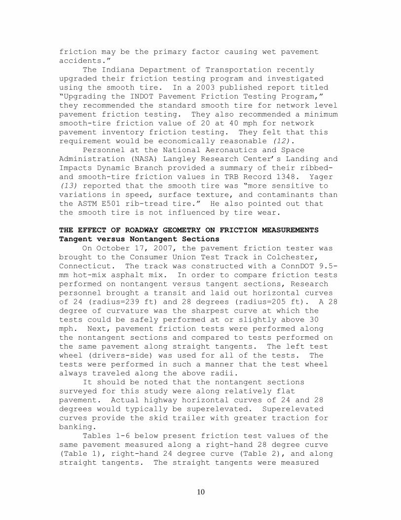
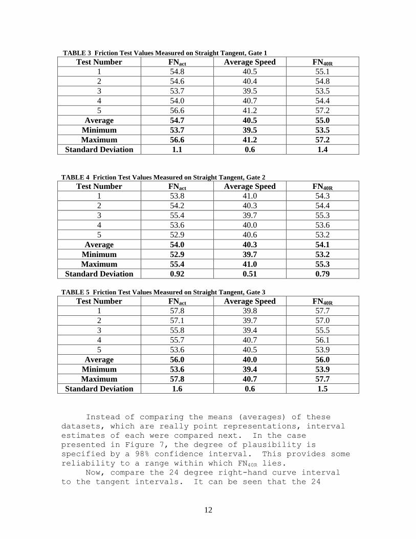
Tables 1-6 below present friction test values of the
same pavement measured along a right-hand 28 degree curve
(Table 1), right-hand 24 degree curve (Table 2), and along
straight tangents. The straight tangents were measured
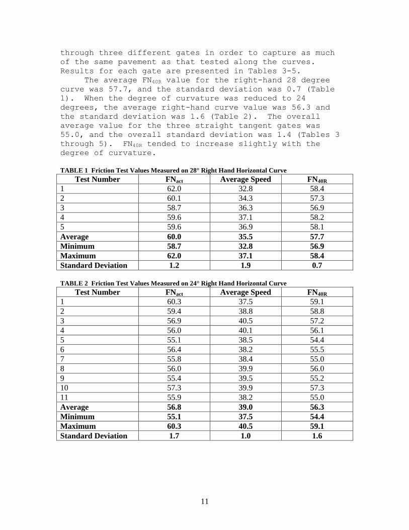
11
through three different gates in order to capture as much
of the same pavement as that tested along the curves.
Results for each gate are presented in Tables 3-5.
The average FN40R value for the right-hand 28 degree
curve was 57.7, and the standard deviation was 0.7 (Table
1). When the degree of curvature was reduced to 24
degrees, the average right-hand curve value was 56.3 and
the standard deviation was 1.6 (Table 2). The overall
average value for the three straight tangent gates was
55.0, and the overall standard deviation was 1.4 (Tables 3
through 5). FN40R tended to increase slightly with the
degree of curvature.
TABLE 1 Friction Test Values Measured on 28° Right Hand Horizontal Curve
Test Number FNact Average Speed FN40R
1 62.0 32.8 58.4
2 60.1 34.3 57.3
3 58.7 36.3 56.9
4 59.6 37.1 58.2
5 59.6 36.9 58.1
Average 60.0 35.5 57.7
Minimum 58.7 32.8 56.9
Maximum 62.0 37.1 58.4
Standard Deviation 1.2 1.9 0.7
TABLE 2 Friction Test Values Measured on 24° Right Hand Horizontal Curve
Test Number FNact Average Speed FN40R
1 60.3 37.5 59.1
2 59.4 38.8 58.8
3 56.9 40.5 57.2
4 56.0 40.1 56.1
5 55.1 38.5 54.4
6 56.4 38.2 55.5
7 55.8 38.4 55.0
8 56.0 39.9 56.0
9 55.4 39.5 55.2
10 57.3 39.9 57.3
11 55.9 38.2 55.0
Average 56.8 39.0 56.3
Minimum 55.1 37.5 54.4
Maximum 60.3 40.5 59.1
Standard Deviation 1.7 1.0 1.6
12
TABLE 3 Friction Test Values Measured on Straight Tangent, Gate 1
Test Number FNact Average Speed FN40R
1 54.8 40.5 55.1
2 54.6 40.4 54.8
3 53.7 39.5 53.5
4 54.0 40.7 54.4
5 56.6 41.2 57.2
Average 54.7 40.5 55.0
Minimum 53.7 39.5 53.5
Maximum 56.6 41.2 57.2
Standard Deviation 1.1 0.6 1.4
TABLE 4 Friction Test Values Measured on Straight Tangent, Gate 2
Test Number FNact Average Speed FN40R
1 53.8 41.0 54.3
2 54.2 40.3 54.4
3 55.4 39.7 55.3
4 53.6 40.0 53.6
5 52.9 40.6 53.2
Average 54.0 40.3 54.1
Minimum 52.9 39.7 53.2
Maximum 55.4 41.0 55.3
Standard Deviation 0.92 0.51 0.79
TABLE 5 Friction Test Values Measured on Straight Tangent, Gate 3
Test Number FNact Average Speed FN40R
1 57.8 39.8 57.7
2 57.1 39.7 57.0
3 55.8 39.4 55.5
4 55.7 40.7 56.1
5 53.6 40.5 53.9
Average 56.0 40.0 56.0
Minimum 53.6 39.4 53.9
Maximum 57.8 40.7 57.7
Standard Deviation 1.6 0.6 1.5
Instead of comparing the means (averages) of these
datasets, which are really point representations, interval
estimates of each were compared next. In the case
presented in Figure 7, the degree of plausibility is
specified by a 98% confidence interval. This provides some
reliability to a range within which FN40R lies.
Now, compare the 24 degree right-hand curve interval
to the tangent intervals. It can be seen that the 24
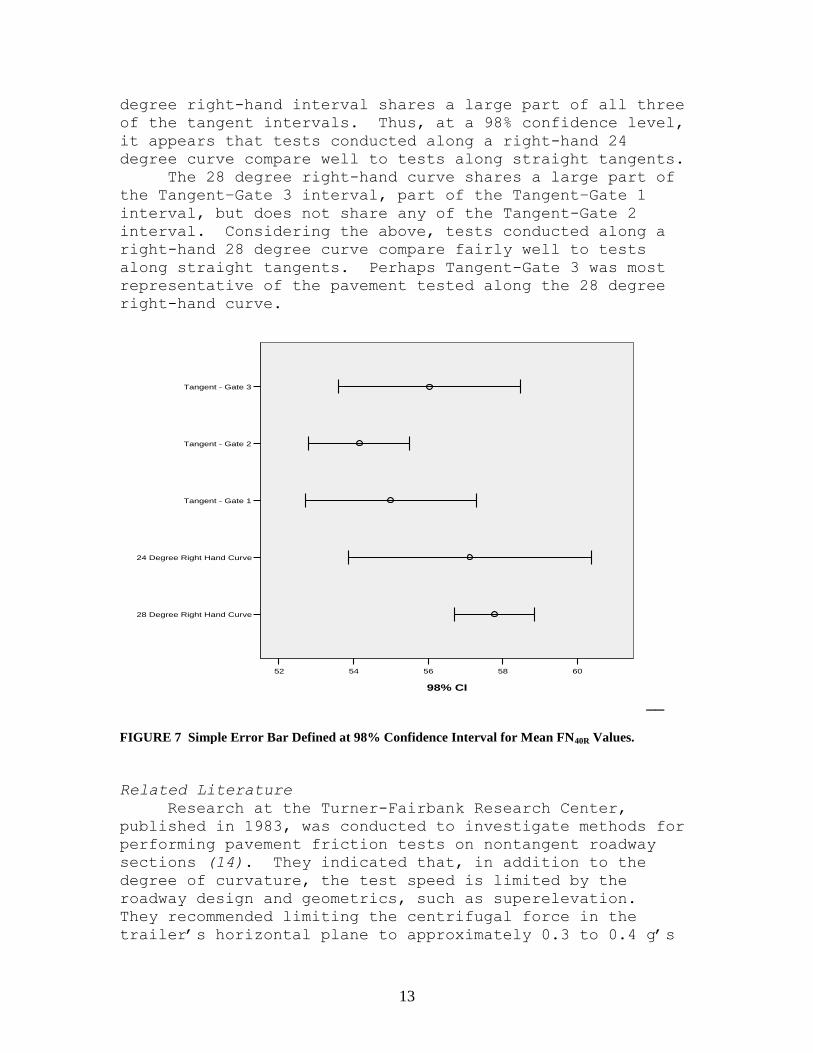
13
degree right-hand interval shares a large part of all three
of the tangent intervals. Thus, at a 98% confidence level,
it appears that tests conducted along a right-hand 24
degree curve compare well to tests along straight tangents.
The 28 degree right-hand curve shares a large part of
the Tangent–Gate 3 interval, part of the Tangent–Gate 1
interval, but does not share any of the Tangent-Gate 2
interval. Considering the above, tests conducted along a
right-hand 28 degree curve compare fairly well to tests
along straight tangents. Perhaps Tangent-Gate 3 was most
representative of the pavement tested along the 28 degree
right-hand curve.
Tangent - Gate 3
Tangent - Gate 2
Tangent - Gate 1
24 Degree Right Hand Curve
28 Degree Right Hand Curve
6058565452
98% CI
__
FIGURE 7 Simple Error Bar Defined at 98% Confidence Interval for Mean FN40R Values.
Related Literature
Research at the Turner-Fairbank Research Center,
published in 1983, was conducted to investigate methods for
performing pavement friction tests on nontangent roadway
sections (14). They indicated that, in addition to the
degree of curvature, the test speed is limited by the
roadway design and geometrics, such as superelevation.
They recommended limiting the centrifugal force in the
trailer’s horizontal plane to approximately 0.3 to 0.4 g’s
14
during locked wheel tests along horizontal curves. This
limiting g-force was determined during dry conditions in
order to keep the unlocked wheel on firm dry pavement,
since the locked wheel has little capacity to provide
restraining side force to keep the trailer from jack-
knifing. They recommended that a Hi-g alarm be installed
to activate system abort circuits in the electronics of the
tester when the horizontal force on the trailer exceeds 0.3
g’s. Finally, they found no significant differences in FN
accuracy when comparing straight tangent versus nontangent
sections of the same pavement as long as they conformed to
the above criteria.
Positive (uphill) versus Negative (downhill) Grades
On September 17, 2007, friction tests were performed
on Route 66 in Marlborough in order to compare tests
performed going uphill versus downhill on the same
pavement. It wasn’t the same exact pavement because
traffic would have to be stopped in order to perform tests
traveling in the opposing direction of traffic, but they
were performed at approximately the same mileposts on the
same route. In order to set-up a truly valid experiment, a
section of pavement would have to be put on a hypothetical
turntable, such as those used in rail yards, in order to
eliminate any directional polarization between tests uphill
versus downhill. This way, the texture of the pavement
would be approached from the same direction. Of course, it
would not be practical or economical to carryout such an
experiment.
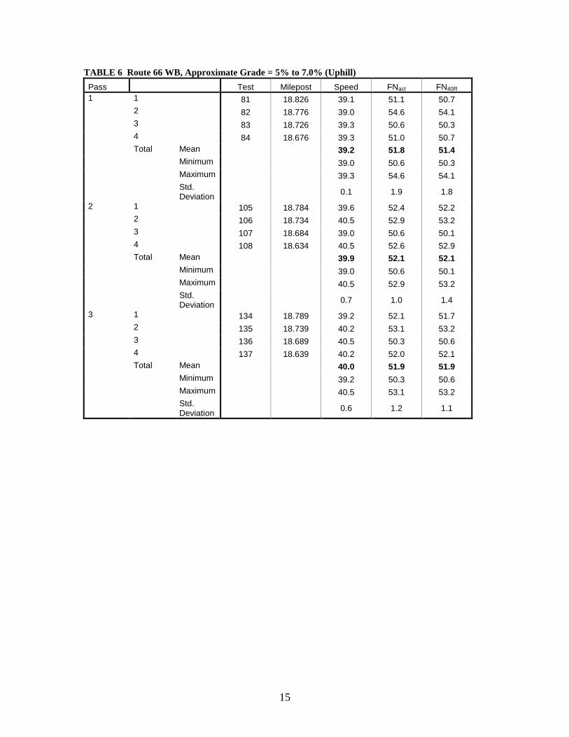
Two hills were compared: one between approximately
18.6 and 18.8 miles (5 to 7% grade) and the other between
19.3 and 19.6 miles (6.5 to 7% grade). For the section
between 18.6 and 18.8 miles, the average FN40R value going
uphill in the westbound direction was 51.8 (see Table 7),
while the average FN40R value going downhill in the
eastbound direction was 46.1 (see Table 8). For the
section between 19.3 and 19.6 miles, the average FN40R value
was 47.0 going uphill in the eastbound direction (Table 9),
and the average FN40R going downhill in the westbound
direction was 46.6 (Table 10). Thus, one section compared
well, while the other did not compare very well.
15
TABLE 6 Route 66 WB, Approximate Grade = 5% to 7.0% (Uphill)
Pass Test Milepost Speed FNact FN40R
1 1 81 18.826 39.1 51.1 50.7
2 82 18.776 39.0 54.6 54.1
3 83 18.726 39.3 50.6 50.3
4 84 18.676 39.3 51.0 50.7
Total Mean 39.2 51.8 51.4
Minimum 39.0 50.6 50.3
Maximum 39.3 54.6 54.1
Std. Deviation
0.1 1.9 1.8
2 1 105 18.784 39.6 52.4 52.2
2 106 18.734 40.5 52.9 53.2
3 107 18.684 39.0 50.6 50.1
4 108 18.634 40.5 52.6 52.9
Total Mean 39.9 52.1 52.1
Minimum 39.0 50.6 50.1
Maximum 40.5 52.9 53.2
Std. Deviation
0.7 1.0 1.4
3 1 134 18.789 39.2 52.1 51.7
2 135 18.739 40.2 53.1 53.2
3 136 18.689 40.5 50.3 50.6
4 137 18.639 40.2 52.0 52.1
Total Mean 40.0 51.9 51.9
Minimum 39.2 50.3 50.6
Maximum 40.5 53.1 53.2
Std. Deviation
0.6 1.2 1.1
16
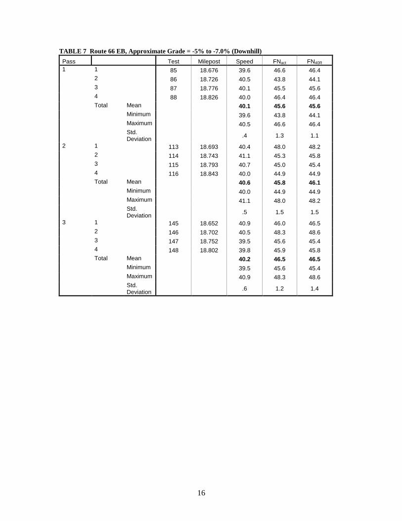
TABLE 7 Route 66 EB, Approximate Grade = -5% to -7.0% (Downhill)
Pass Test Milepost Speed FNact FN40R
1 1 85 18.676 39.6 46.6 46.4
2 86 18.726 40.5 43.8 44.1
3 87 18.776 40.1 45.5 45.6
4 88 18.826 40.0 46.4 46.4
Total Mean 40.1 45.6 45.6
Minimum 39.6 43.8 44.1
Maximum 40.5 46.6 46.4
Std. Deviation
.4 1.3 1.1
2 1 113 18.693 40.4 48.0 48.2
2 114 18.743 41.1 45.3 45.8
3 115 18.793 40.7 45.0 45.4
4 116 18.843 40.0 44.9 44.9
Total Mean 40.6 45.8 46.1
Minimum 40.0 44.9 44.9
Maximum 41.1 48.0 48.2
Std. Deviation
.5 1.5 1.5
3 1 145 18.652 40.9 46.0 46.5
2 146 18.702 40.5 48.3 48.6
3 147 18.752 39.5 45.6 45.4
4 148 18.802 39.8 45.9 45.8
Total Mean 40.2 46.5 46.5
Minimum 39.5 45.6 45.4
Maximum 40.9 48.3 48.6
Std. Deviation
.6 1.2 1.4
17
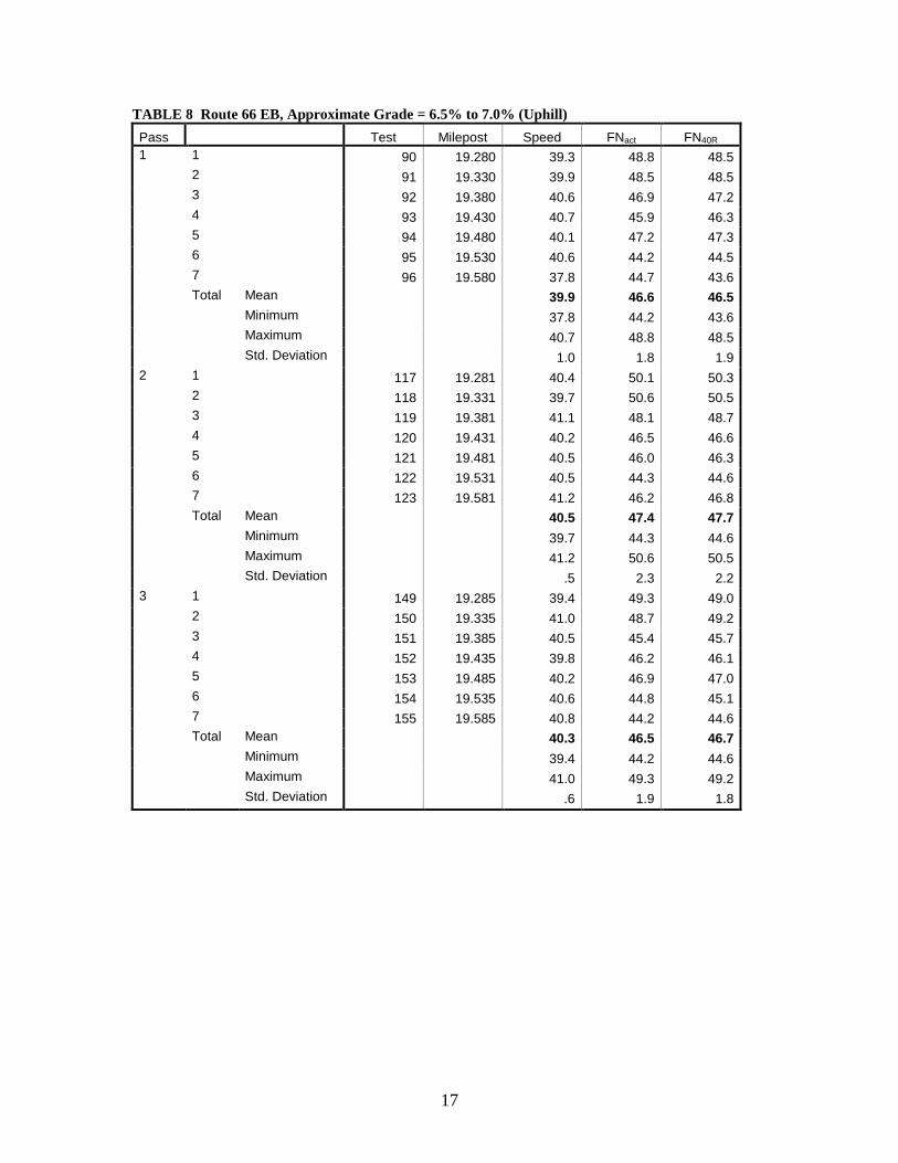
TABLE 8 Route 66 EB, Approximate Grade = 6.5% to 7.0% (Uphill)
Pass Test Milepost Speed FNact FN40R
1 1 90 19.280 39.3 48.8 48.5
2 91 19.330 39.9 48.5 48.5
3 92 19.380 40.6 46.9 47.2
4 93 19.430 40.7 45.9 46.3
5 94 19.480 40.1 47.2 47.3
6 95 19.530 40.6 44.2 44.5
7 96 19.580 37.8 44.7 43.6
Total Mean 39.9 46.6 46.5
Minimum 37.8 44.2 43.6
Maximum 40.7 48.8 48.5
Std. Deviation 1.0 1.8 1.9
2 1 117 19.281 40.4 50.1 50.3
2 118 19.331 39.7 50.6 50.5
3 119 19.381 41.1 48.1 48.7
4 120 19.431 40.2 46.5 46.6
5 121 19.481 40.5 46.0 46.3
6 122 19.531 40.5 44.3 44.6
7 123 19.581 41.2 46.2 46.8
Total Mean 40.5 47.4 47.7
Minimum 39.7 44.3 44.6
Maximum 41.2 50.6 50.5
Std. Deviation .5 2.3 2.2
3 1 149 19.285 39.4 49.3 49.0
2 150 19.335 41.0 48.7 49.2
3 151 19.385 40.5 45.4 45.7
4 152 19.435 39.8 46.2 46.1
5 153 19.485 40.2 46.9 47.0
6 154 19.535 40.6 44.8 45.1
7 155 19.585 40.8 44.2 44.6
Total Mean 40.3 46.5 46.7
Minimum 39.4 44.2 44.6
Maximum 41.0 49.3 49.2
Std. Deviation .6 1.9 1.8
18
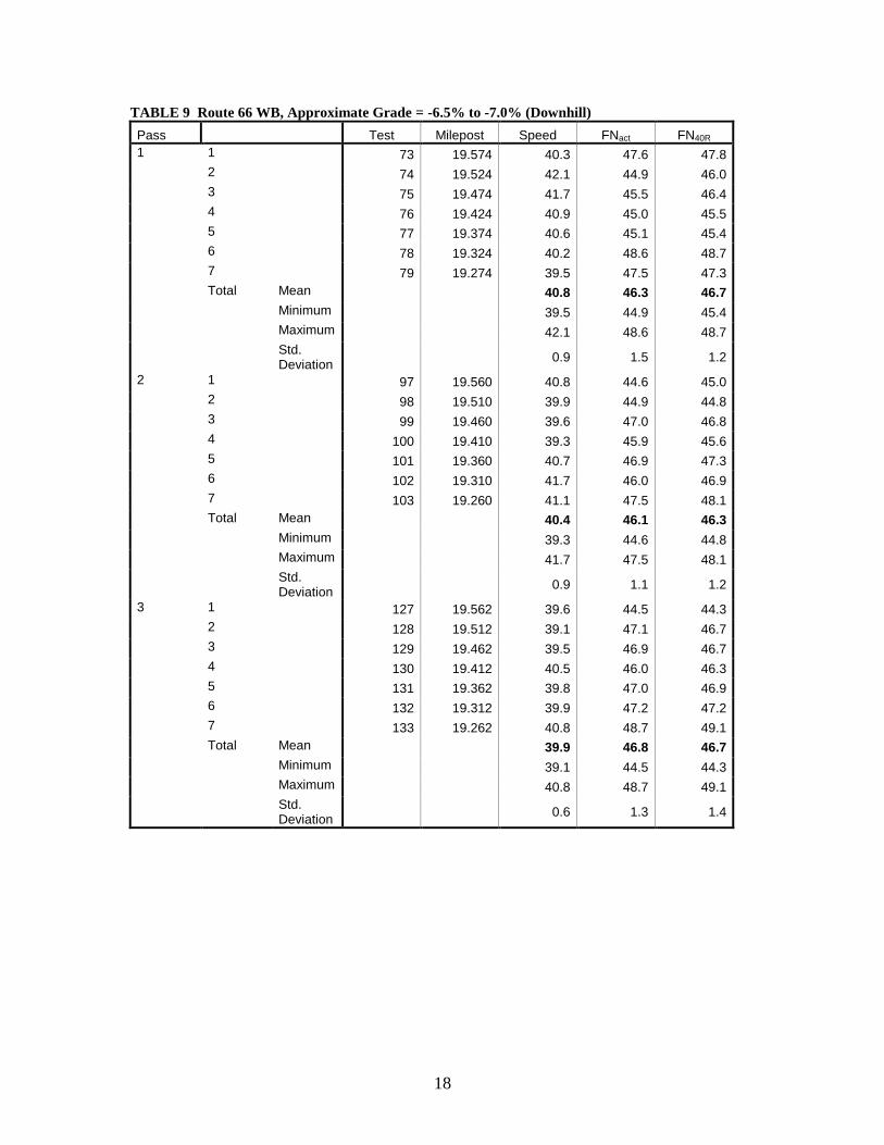
TABLE 9 Route 66 WB, Approximate Grade = -6.5% to -7.0% (Downhill)
Pass Test Milepost Speed FNact FN40R
1 1 73 19.574 40.3 47.6 47.8
2 74 19.524 42.1 44.9 46.0
3 75 19.474 41.7 45.5 46.4
4 76 19.424 40.9 45.0 45.5
5 77 19.374 40.6 45.1 45.4
6 78 19.324 40.2 48.6 48.7
7 79 19.274 39.5 47.5 47.3
Total Mean 40.8 46.3 46.7
Minimum 39.5 44.9 45.4
Maximum 42.1 48.6 48.7
Std. Deviation
0.9 1.5 1.2
2 1 97 19.560 40.8 44.6 45.0
2 98 19.510 39.9 44.9 44.8
3 99 19.460 39.6 47.0 46.8
4 100 19.410 39.3 45.9 45.6
5 101 19.360 40.7 46.9 47.3
6 102 19.310 41.7 46.0 46.9
7 103 19.260 41.1 47.5 48.1
Total Mean 40.4 46.1 46.3
Minimum 39.3 44.6 44.8
Maximum 41.7 47.5 48.1
Std. Deviation
0.9 1.1 1.2
3 1 127 19.562 39.6 44.5 44.3
2 128 19.512 39.1 47.1 46.7
3 129 19.462 39.5 46.9 46.7
4 130 19.412 40.5 46.0 46.3
5 131 19.362 39.8 47.0 46.9
6 132 19.312 39.9 47.2 47.2
7 133 19.262 40.8 48.7 49.1
Total Mean 39.9 46.8 46.7
Minimum 39.1 44.5 44.3
Maximum 40.8 48.7 49.1
Std. Deviation
0.6 1.3 1.4
19
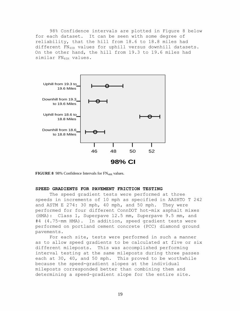
98% Confidence intervals are plotted in Figure 8 below
for each dataset. It can be seen with some degree of
reliability, that the hill from 18.6 to 18.8 miles had
different FN40R values for uphill versus downhill datasets.
On the other hand, the hill from 19.3 to 19.6 miles had
similar FN40R values.
Uphill from 19.3 to
19.6 Miles
Downhill from 19.3
to 19.6 Miles
Uphill from 18.6 to
18.8 Miles
Downhill from 18.6
to 18.8 Miles
52504846
98% CI
FIGURE 8 98% Confidence Intervals for FN40R values.
SPEED GRADIENTS FOR PAVEMENT FRICTION TESTING
The speed gradient tests were performed at three
speeds in increments of 10 mph as specified in AASHTO T 242
and ASTM E 274: 30 mph, 40 mph, and 50 mph. They were
performed for four different ConnDOT hot-mix asphalt mixes
(HMA): Class 1, Superpave 12.5 mm, Superpave 9.5 mm, and
#4 (4.75-mm HMA). In addition, speed gradient tests were
performed on portland cement concrete (PCC) diamond ground
pavements.
For each site, tests were performed in such a manner
as to allow speed gradients to be calculated at five or six
different mileposts. This was accomplished performing
interval testing at the same mileposts during three passes
each at 30, 40, and 50 mph. This proved to be worthwhile
because the speed-gradient slopes at the individual
mileposts corresponded better than combining them and
determining a speed-gradient slope for the entire site.
20
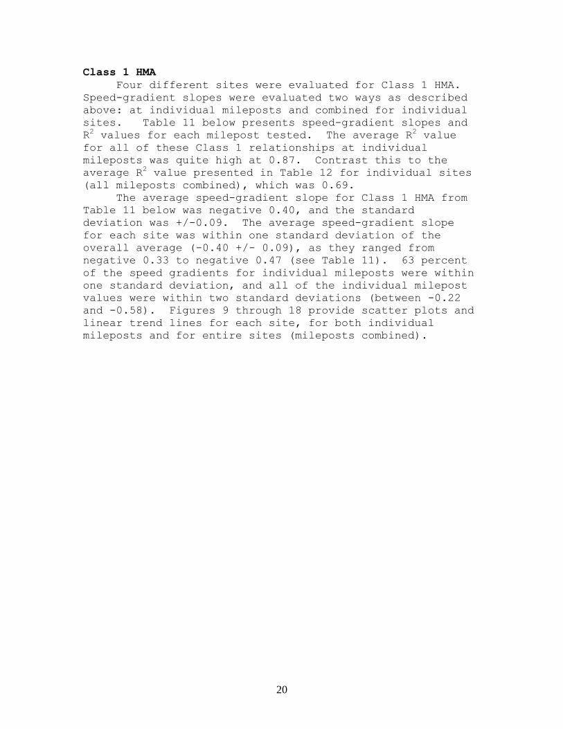
Class 1 HMA
Four different sites were evaluated for Class 1 HMA.
Speed-gradient slopes were evaluated two ways as described
above: at individual mileposts and combined for individual
sites. Table 11 below presents speed-gradient slopes and
R2 values for each milepost tested. The average R
2 value
for all of these Class 1 relationships at individual
mileposts was quite high at 0.87. Contrast this to the
average R2 value presented in Table 12 for individual sites
(all mileposts combined), which was 0.69.
The average speed-gradient slope for Class 1 HMA from
Table 11 below was negative 0.40, and the standard
deviation was +/-0.09. The average speed-gradient slope
for each site was within one standard deviation of the
overall average (-0.40 +/- 0.09), as they ranged from
negative 0.33 to negative 0.47 (see Table 11). 63 percent
of the speed gradients for individual mileposts were within
one standard deviation, and all of the individual milepost
values were within two standard deviations (between -0.22
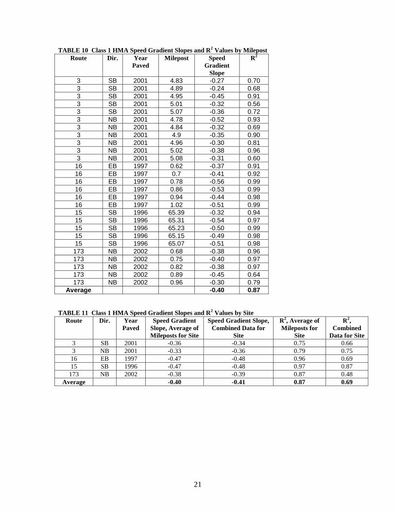
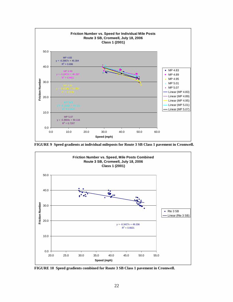
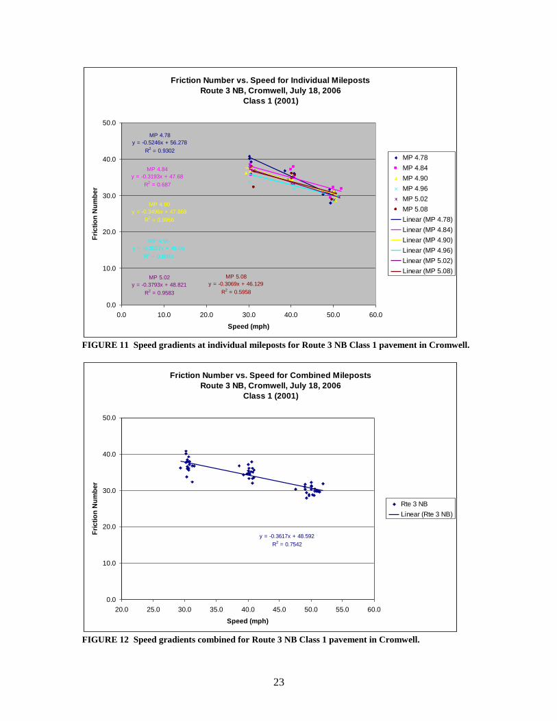
and -0.58). Figures 9 through 18 provide scatter plots and
linear trend lines for each site, for both individual
mileposts and for entire sites (mileposts combined).
21
TABLE 10 Class 1 HMA Speed Gradient Slopes and R2 Values by Milepost
Route Dir. Year
Paved
Milepost Speed
Gradient
Slope
R2
3 SB 2001 4.83 -0.27 0.70
3 SB 2001 4.89 -0.24 0.68
3 SB 2001 4.95 -0.45 0.91
3 SB 2001 5.01 -0.32 0.56
3 SB 2001 5.07 -0.36 0.72
3 NB 2001 4.78 -0.52 0.93
3 NB 2001 4.84 -0.32 0.69
3 NB 2001 4.9 -0.35 0.90
3 NB 2001 4.96 -0.30 0.81
3 NB 2001 5.02 -0.38 0.96
3 NB 2001 5.08 -0.31 0.60
16 EB 1997 0.62 -0.37 0.91
16 EB 1997 0.7 -0.41 0.92
16 EB 1997 0.78 -0.56 0.99
16 EB 1997 0.86 -0.53 0.99
16 EB 1997 0.94 -0.44 0.98
16 EB 1997 1.02 -0.51 0.99
15 SB 1996 65.39 -0.32 0.94
15 SB 1996 65.31 -0.54 0.97
15 SB 1996 65.23 -0.50 0.99
15 SB 1996 65.15 -0.49 0.98
15 SB 1996 65.07 -0.51 0.98
173 NB 2002 0.68 -0.38 0.96
173 NB 2002 0.75 -0.40 0.97
173 NB 2002 0.82 -0.38 0.97
173 NB 2002 0.89 -0.45 0.64
173 NB 2002 0.96 -0.30 0.79
Average -0.40 0.87
TABLE 11 Class 1 HMA Speed Gradient Slopes and R2 Values by Site
Route Dir. Year
Paved
Speed Gradient
Slope, Average of
Mileposts for Site
Speed Gradient Slope,
Combined Data for
Site
R2, Average of
Mileposts for
Site
R2,
Combined
Data for Site
3 SB 2001 -0.36 -0.34 0.75 0.66
3 NB 2001 -0.33 -0.36 0.79 0.75
16 EB 1997 -0.47 -0.48 0.96 0.69
15 SB 1996 -0.47 -0.48 0.97 0.87
173 NB 2002 -0.38 -0.39 0.87 0.48
Average -0.40 -0.41 0.87 0.69
22
Friction Number vs. Speed for Individual Mile Posts
Route 3 SB, Cromwell, July 18, 2006
Class 1 (2001)
MP 4.83
y = -0.2667x + 45.304
R2 = 0.696
MP 4.89
y = -0.2407x + 46.267
R2 = 0.6811
MP 4.95
y = -0.4536x + 52.929
R2 = 0.9138
MP 5.01
y = -0.3181x + 49.325
R2 = 0.5644
MP 5.07
y = -0.3604x + 50.116
R2 = 0.7207
0.0
10.0
20.0
30.0
40.0
50.0
0.0 10.0 20.0 30.0 40.0 50.0 60.0
Speed (mph)
Fri
cti
on
Nu
mb
er
MP 4.83
MP 4.89
MP 4.95
MP 5.01
MP 5.07
Linear (MP 4.83)
Linear (MP 4.89)
Linear (MP 4.95)
Linear (MP 5.01)
Linear (MP 5.07)
FIGURE 9 Speed gradients at individual mileposts for Route 3 SB Class 1 pavement in Cromwell.
Friction Number vs. Speed, Mile Posts Combined
Route 3 SB, Cromwell, July 18, 2006
Class 1 (2001)
y = -0.3427x + 49.336
R2 = 0.6621
0.0
10.0
20.0
30.0
40.0
50.0
20.0 25.0 30.0 35.0 40.0 45.0 50.0 55.0
Speed (mph)
Fri
cti
on
Nu
mb
er
Rte 3 SB
Linear (Rte 3 SB)
FIGURE 10 Speed gradients combined for Route 3 SB Class 1 pavement in Cromwell.
23
Friction Number vs. Speed for Individual Mileposts
Route 3 NB, Cromwell, July 18, 2006
Class 1 (2001)
MP 4.78
y = -0.5246x + 56.278
R2 = 0.9302
MP 4.84
y = -0.3193x + 47.68
R2 = 0.687
MP 4.90
y = -0.3496x + 47.868
R2 = 0.8966
MP 4.96
y = -0.3027x + 45.05
R2 = 0.8093
MP 5.02
y = -0.3793x + 48.821
R2 = 0.9583
MP 5.08
y = -0.3069x + 46.129
R2 = 0.5958
0.0
10.0
20.0
30.0
40.0
50.0
0.0 10.0 20.0 30.0 40.0 50.0 60.0
Speed (mph)
Fri
cti
on
Nu
mb
er
MP 4.78
MP 4.84
MP 4.90
MP 4.96
MP 5.02
MP 5.08
Linear (MP 4.78)
Linear (MP 4.84)
Linear (MP 4.90)
Linear (MP 4.96)
Linear (MP 5.02)
Linear (MP 5.08)
FIGURE 11 Speed gradients at individual mileposts for Route 3 NB Class 1 pavement in Cromwell.
Friction Number vs. Speed for Combined Mileposts
Route 3 NB, Cromwell, July 18, 2006
Class 1 (2001)
y = -0.3617x + 48.592
R2 = 0.7542
0.0
10.0
20.0
30.0
40.0
50.0
20.0 25.0 30.0 35.0 40.0 45.0 50.0 55.0 60.0
Speed (mph)
Fri
cti
on
Nu
mb
er
Rte 3 NB
Linear (Rte 3 NB)
FIGURE 12 Speed gradients combined for Route 3 NB Class 1 pavement in Cromwell.
24
Friction Number vs. Speed for Individual Mile Posts
Route 16 EB, East Hampton, September 27, 2006
Class 1 (1997)
MP 0.62
y = -0.3702x + 59.87
R2 = 0.9062
MP 0.70
y = -0.414x + 67.966
R2 = 0.9246
MP 0.78
y = -0.5552x + 73.08
R2 = 0.9853
MP 0.86
y = -0.526x + 73.509
R2 = 0.9875
MP 0.94
y = -0.4439x + 69.187
R2 = 0.9795
MP 1.02
y = -0.5128x + 71.392
R2 = 0.9940.0
10.0
20.0
30.0
40.0
50.0
60.0
70.0
0.0 10.0 20.0 30.0 40.0 50.0 60.0
Speed (mph)
Fri
cti
on
Nu
mb
er
MP 0.62
MP 0.70
MP 0.78
MP 0.86
MP 0.94
MP 1.02
Linear (MP 0.62)
Linear (MP 0.70)
Linear (MP 0.78)
Linear (MP 0.86)
Linear (MP 0.94)
Linear (MP 1.02)
FIGURE 13 Speed gradients at individual mileposts for Route 16 EB Class 1 pavement in East
Hampton.
Friction Number vs. Speed, Mile Posts Combined
Rte 16 EB, East Hampton, September 27, 2006
Class 1 (1997)
y = -0.4755x + 69.374
R2 = 0.6903
0.0
10.0
20.0
30.0
40.0
50.0
60.0
70.0
20.0 25.0 30.0 35.0 40.0 45.0 50.0 55.0 60.0
Speed (mph)
Fri
cti
on
Nu
mb
er
Rte 16 EB
Linear (Rte 16 EB)
FIGURE 14 Speed gradients combined for Route 16 EB Class 1 pavement in East Hampton.
25
Friction Number vs. Speed for Individual Mileposts
Rte 15 SB, Meriden, October 11, 2006
Class 1 (1996)
MP 65.39
y = -0.3242x + 61.616
R2 = 0.9357
MP 65.31
y = -0.5365x + 71.732
R2 = 0.9748
MP 65.23
y = -0.5001x + 67.948
R2 = 0.9923
MP 65.15
y = -0.4917x + 68.94
R2 = 0.9764
MP 65.07
y = -0.5081x + 66.971
R2 = 0.9753
0.0
10.0
20.0
30.0
40.0
50.0
60.0
0.0 10.0 20.0 30.0 40.0 50.0 60.0
Speed (mph)
Fri
cti
on
Nu
mb
er
MP 65.39
MP 65.31
MP 65.23
MP 65.15
MP 65.07
Linear (MP 65.39)
Linear (MP 65.31)
Linear (MP 65.23)
Linear (MP 65.15)
Linear (MP 65.07)
FIGURE 15 Speed gradients at individual mileposts for Route 15 SB Class 1 pavement in Meriden.
Friction Number vs. Speed for Combined Mileposts
Rte 15 SB, Meriden, October 11, 2006
Class 1 (1996)
y = -0.4758x + 67.584
R2 = 0.8677
0.0
10.0
20.0
30.0
40.0
50.0
60.0
20.0 25.0 30.0 35.0 40.0 45.0 50.0 55.0 60.0
Speed (mph)
Fri
cti
on
Nu
mb
er
Rte 15 SB
Linear (Rte 15 SB)
FIGURE 16 Speed gradients combined for Route 15 SB Class 1 pavement in Meriden.
26
Friction Number vs. Speed for Individual Mileposts
Route 173 NB, Newington, October 26, 2006
Class 1 (2002)
MP 0.68
y = -0.3753x + 48.672
R2 = 0.9639
MP 0.75
y = -0.4043x + 53.22
R2 = 0.9681
MP 0.82
y = -0.3812x + 50.785
R2 = 0.9658
MP 0.89
y = -0.4533x + 60.103
R2 = 0.6353
MP 0.96
y = -0.297x + 50.123
R2 = 0.789
0.0
10.0
20.0
30.0
40.0
50.0
60.0
0.0 10.0 20.0 30.0 40.0 50.0 60.0
Speed (mph)
Fri
cti
on
Nu
mb
er
MP 0.68
MP 0.75
MP 0.82
MP 0.89
MP 0.96
Linear (MP 0.68)
Linear (MP 0.75)
Linear (MP 0.82)
Linear (MP 0.89)
Linear (MP 0.96)
FIGURE 17 Speed gradients at individual mileposts for Route 173 NB Class pavement in
Newington.
Friction Number vs. Speed for Combined Mileposts
Route 173 NB, Newington, October 26, 2006
Class 1 (2002)
y = -0.3862x + 52.743
R2 = 0.4781
0.0
10.0
20.0
30.0
40.0
50.0
60.0
20.0 25.0 30.0 35.0 40.0 45.0 50.0 55.0
Speed (mph)
Fri
cti
on
Nu
mb
er
Rte 173 NB
Linear (Rte 173 NB)
FIGURE 18 Speed gradients combined for Route 173 NB Class 1 pavement in Newington.

27
Figure 19 below presents a simple error bar chart,
where the bars represent 98% confidence intervals (CI) for
each location. That is to say, there is 98 percent
likelihood that the range of values represented by the bars
includes the population mean for each location. The red
vertical line represents the speed gradient currently used
by ConnDOT (-0.50) for calculating FN40R. The green
vertical line is located at the average speed gradient for
the individual sites (negative 0.40). It can be seen that
the red vertical line falls within the 98% CI for only two
of the five locations. Therefore, for the Class 1 HMA,
negative 0.50 wouldn’t be the most representative speed
gradient for calculating FN40R.
What would the consequences be of using -0.50 when the
actual gradient is -0.40 for example? Let’s calculate FN40R
for a FN value of 40 measured at 30 mph. Using -0.50, FN40R
would be 35.0. Using a more representative speed gradient
of -0.40 in this hypothetical scenario, FN40R would be 36.0.
A more conservative FN40R value was calculated in this
instance. Now, let’s calculate FN40R for a FN value of 40
measured at 50 mph. Using -0.50 in this case, FN40R would
be 45. Next, using -0.40, FN40R would be 44. A non-
conservative FN40R value was calculated in this case.
Route 3 SB
Route 3 NB
Route 173 NB
Route 16 EB
Route 15 SB
Des
crip
tion
0.0-0.2-0.4-0.6-0.8
98% CI Speed Gradient
FIGURE 19 98% Confidence intervals for speed gradients for Class 1 pavements.
28
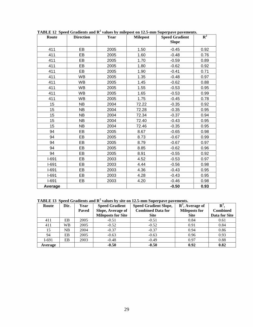
12.5-mm Superpave HMA
Speed-gradient slopes were determined for four
different sites for the Superpave 12.5-mm HMA. These
included Route 411 in Rocky Hill EB and WB, Route 15 NB in
Berlin, Route 94 in Hebron, and Interstate 691 in Meriden.
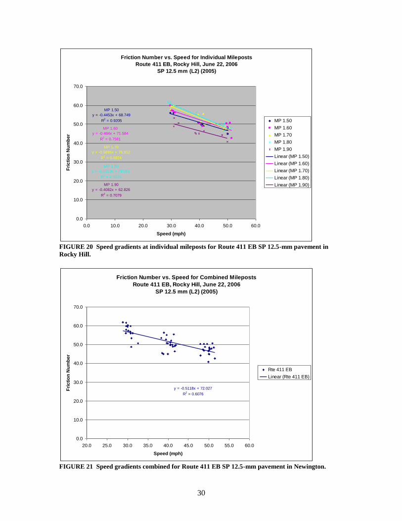
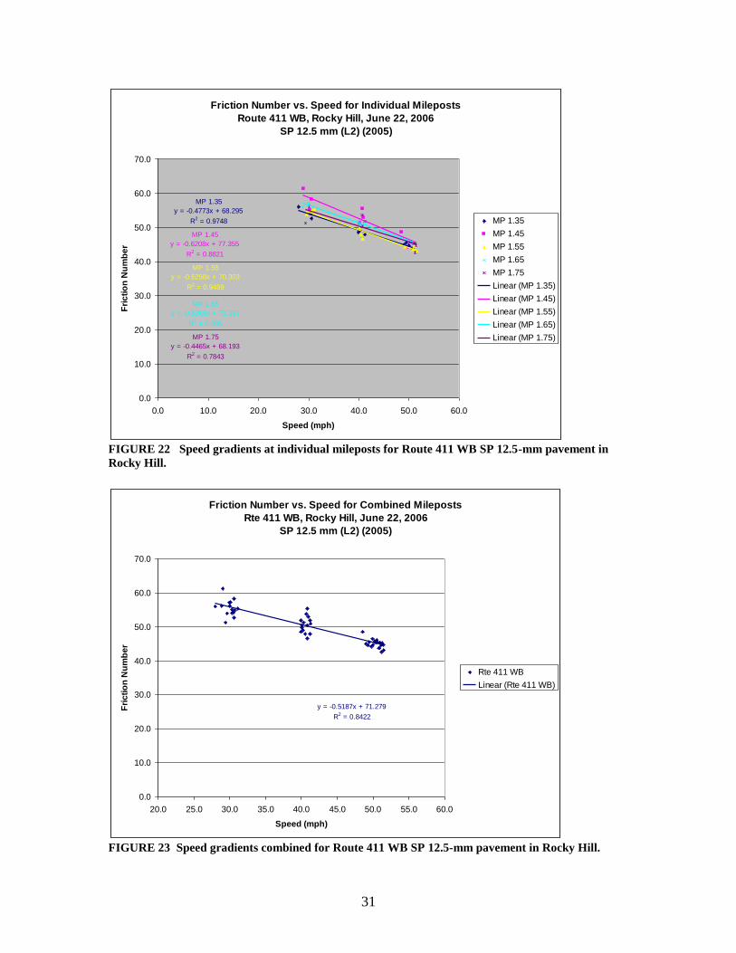
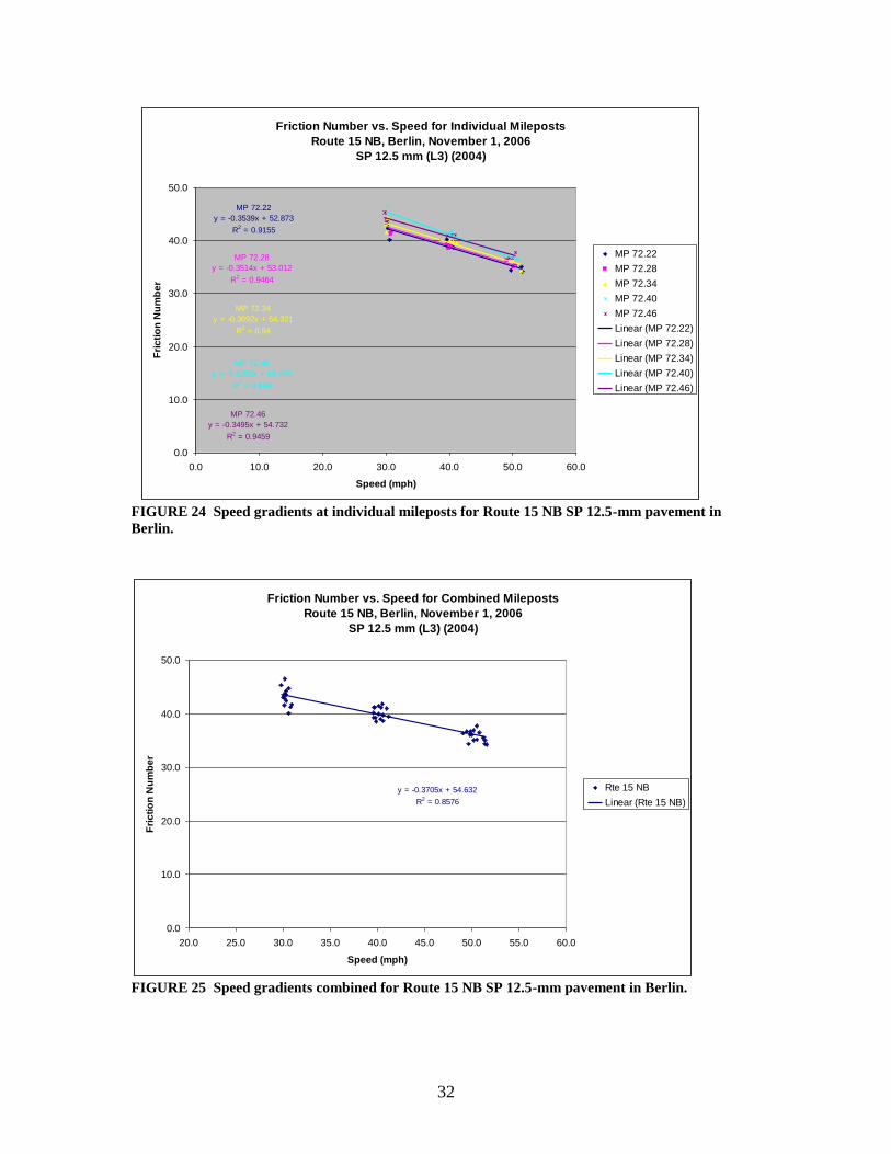
Trend line data for each milepost are presented in Table
13. Figures 20 through 29 provide scatter plots and linear
trend lines for each site, for both individual mileposts
and for entire sites.
The average speed-gradient slope for individual
mileposts was -0.50, and the standard deviation was +/-
0.10. Therefore, the actual average gradient (-0.50) was
equal to the assumed value (-0.50) used to calculate FN40R.
The values ranged between -0.35 and -0.67. 60 percent of
the values were within one standard deviation of the mean
(-0.40 to -0.60), and all of the values were within two
standard deviations of the mean (-0.30 to -0.70). The
average R2 value was 0.93, so there was a strong linear
tendency between friction numbers and speed for the
individual mileposts.
29
TABLE 12 Speed Gradients and R2 values by milepost on 12.5-mm Superpave pavements.
Route Direction Year Milepost Speed Gradient
Slope
R2
411 EB 2005 1.50 -0.45 0.92
411 EB 2005 1.60 -0.48 0.76
411 EB 2005 1.70 -0.59 0.89
411 EB 2005 1.80 -0.62 0.92
411 EB 2005 1.90 -0.41 0.71
411 WB 2005 1.35 -0.48 0.97
411 WB 2005 1.45 -0.62 0.88
411 WB 2005 1.55 -0.53 0.95
411 WB 2005 1.65 -0.53 0.99
411 WB 2005 1.75 -0.45 0.78
15 NB 2004 72.22 -0.35 0.92
15 NB 2004 72.28 -0.35 0.95
15 NB 2004 72.34 -0.37 0.94
15 NB 2004 72.40 -0.43 0.95
15 NB 2004 72.46 -0.35 0.95
94 EB 2005 8.67 -0.65 0.98
94 EB 2005 8.73 -0.67 0.99
94 EB 2005 8.79 -0.67 0.97
94 EB 2005 8.85 -0.62 0.96
94 EB 2005 8.91 -0.55 0.92
I-691 EB 2003 4.52 -0.53 0.97
I-691 EB 2003 4.44 -0.56 0.98
I-691 EB 2003 4.36 -0.43 0.95
I-691 EB 2003 4.28 -0.43 0.95
I-691 EB 2003 4.20 -0.46 0.98
Average -0.50 0.93
TABLE 13 Speed Gradients and R2 values by site on 12.5-mm Superpave pavements.
Route Dir. Year
Paved
Speed Gradient
Slope, Average of
Mileposts for Site
Speed Gradient Slope,
Combined Data for
Site
R2, Average of
Mileposts for
Site
R2,
Combined
Data for Site
411 EB 2005 -0.51 -0.51 0.84 0.61
411 WB 2005 -0.52 -0.52 0.91 0.84
15 NB 2004 -0.37 -0.37 0.94 0.86
94 EB 2005 -0.63 -0.63 0.96 0.93
I-691 EB 2003 -0.48 -0.49 0.97 0.88
Average -0.50 -0.50 0.92 0.82
30
Friction Number vs. Speed for Individual Mileposts
Route 411 EB, Rocky Hill, June 22, 2006
SP 12.5 mm (L2) (2005)
MP 1.50
y = -0.4453x + 68.749
R2 = 0.9205
MP 1.60
y = -0.484x + 71.584
R2 = 0.7581
MP 1.70
y = -0.5896x + 76.912
R2 = 0.8924
MP 1.80
y = -0.6213x + 79.081
R2 = 0.9225
MP 1.90
y = -0.4082x + 62.826
R2 = 0.7079
0.0
10.0
20.0
30.0
40.0
50.0
60.0
70.0
0.0 10.0 20.0 30.0 40.0 50.0 60.0
Speed (mph)
Fri
cti
on
Nu
mb
er
MP 1.50
MP 1.60
MP 1.70
MP 1.80
MP 1.90
Linear (MP 1.50)
Linear (MP 1.60)
Linear (MP 1.70)
Linear (MP 1.80)
Linear (MP 1.90)
FIGURE 20 Speed gradients at individual mileposts for Route 411 EB SP 12.5-mm pavement in
Rocky Hill.
Friction Number vs. Speed for Combined Mileposts
Route 411 EB, Rocky Hill, June 22, 2006
SP 12.5 mm (L2) (2005)
y = -0.5118x + 72.027
R2 = 0.6076
0.0
10.0
20.0
30.0
40.0
50.0
60.0
70.0
20.0 25.0 30.0 35.0 40.0 45.0 50.0 55.0 60.0
Speed (mph)
Fri
cti
on
Nu
mb
er
Rte 411 EB
Linear (Rte 411 EB)
FIGURE 21 Speed gradients combined for Route 411 EB SP 12.5-mm pavement in Newington.
31
Friction Number vs. Speed for Individual Mileposts
Route 411 WB, Rocky Hill, June 22, 2006
SP 12.5 mm (L2) (2005)
MP 1.35
y = -0.4773x + 68.295
R2 = 0.9748
MP 1.45
y = -0.6208x + 77.355
R2 = 0.8821
MP 1.55
y = -0.5258x + 70.303
R2 = 0.9459
MP 1.65
y = -0.5269x + 72.397
R2 = 0.985
MP 1.75
y = -0.4465x + 68.193
R2 = 0.7843
0.0
10.0
20.0
30.0
40.0
50.0
60.0
70.0
0.0 10.0 20.0 30.0 40.0 50.0 60.0
Speed (mph)
Fri
cti
on
Nu
mb
er
MP 1.35
MP 1.45
MP 1.55
MP 1.65
MP 1.75
Linear (MP 1.35)
Linear (MP 1.45)
Linear (MP 1.55)
Linear (MP 1.65)
Linear (MP 1.75)
FIGURE 22 Speed gradients at individual mileposts for Route 411 WB SP 12.5-mm pavement in
Rocky Hill.
Friction Number vs. Speed for Combined Mileposts
Rte 411 WB, Rocky Hill, June 22, 2006
SP 12.5 mm (L2) (2005)
y = -0.5187x + 71.279
R2 = 0.8422
0.0
10.0
20.0
30.0
40.0
50.0
60.0
70.0
20.0 25.0 30.0 35.0 40.0 45.0 50.0 55.0 60.0
Speed (mph)
Fri
cti
on
Nu
mb
er
Rte 411 WB
Linear (Rte 411 WB)
FIGURE 23 Speed gradients combined for Route 411 WB SP 12.5-mm pavement in Rocky Hill.
32
Friction Number vs. Speed for Individual Mileposts
Route 15 NB, Berlin, November 1, 2006
SP 12.5 mm (L3) (2004)
MP 72.22
y = -0.3539x + 52.873
R2 = 0.9155
MP 72.28
y = -0.3514x + 53.012
R2 = 0.9464
MP 72.34
y = -0.3692x + 54.321
R2 = 0.94
MP 72.40
y = -0.4253x + 58.095
R2 = 0.949
MP 72.46
y = -0.3495x + 54.732
R2 = 0.9459
0.0
10.0
20.0
30.0
40.0
50.0
0.0 10.0 20.0 30.0 40.0 50.0 60.0
Speed (mph)
Fri
cti
on
Nu
mb
er
MP 72.22
MP 72.28
MP 72.34
MP 72.40
MP 72.46
Linear (MP 72.22)
Linear (MP 72.28)
Linear (MP 72.34)
Linear (MP 72.40)
Linear (MP 72.46)
FIGURE 24 Speed gradients at individual mileposts for Route 15 NB SP 12.5-mm pavement in
Berlin.
Friction Number vs. Speed for Combined Mileposts
Route 15 NB, Berlin, November 1, 2006
SP 12.5 mm (L3) (2004)
y = -0.3705x + 54.632
R2 = 0.8576
0.0
10.0
20.0
30.0
40.0
50.0
20.0 25.0 30.0 35.0 40.0 45.0 50.0 55.0 60.0
Speed (mph)
Fri
cti
on
Nu
mb
er
Rte 15 NB
Linear (Rte 15 NB)
FIGURE 25 Speed gradients combined for Route 15 NB SP 12.5-mm pavement in Berlin.
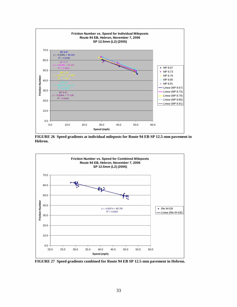
33
Friction Number vs. Speed for Individual Mileposts
Route 94 EB, Hebron, November 7, 2006
SP 12.5mm (L2) (2005)
MP 8.67
y = -0.6455x + 80.104
R2 = 0.9769
MP 8.73
y = -0.6746x + 83.204
R2 = 0.9854
MP 8.79
y = -0.6676x + 81.999
R2 = 0.9674
MP 8.85
y = -0.6174x + 81.389
R2 = 0.9607
MP 8.91
y = -0.5549x + 77.139
R2 = 0.9245
0.0
10.0
20.0
30.0
40.0
50.0
60.0
70.0
0.0 10.0 20.0 30.0 40.0 50.0 60.0
Speed (mph)
Fri
cti
on
Nu
mb
er
MP 8.67
MP 8.73
MP 8.79
MP 8.85
MP 8.91
Linear (MP 8.67)
Linear (MP 8.73)
Linear (MP 8.79)
Linear (MP 8.85)
Linear (MP 8.91)
FIGURE 26 Speed gradients at individual mileposts for Route 94 EB SP 12.5-mm pavement in
Hebron.
Friction Number vs. Speed for Combined Mileposts
Route 94 EB, Hebron, November 7, 2006
SP 12.5mm (L2) (2005)
y = -0.6317x + 80.755
R2 = 0.9342
0.0
10.0
20.0
30.0
40.0
50.0
60.0
70.0
20.0 25.0 30.0 35.0 40.0 45.0 50.0 55.0 60.0
Speed (mph)
Fri
cti
on
Nu
mb
er
Rte 94 EB
Linear (Rte 94 EB)
FIGURE 27 Speed gradients combined for Route 94 EB SP 12.5-mm pavement in Hebron.
34
Friction Number vs. Speed for Individual Mileposts
Interstate 691 EB, Meriden, November 15, 2006
SP 12.5mm (L3) (2003)
MP 4.52
y = -0.5276x + 75.658
R2 = 0.9743
MP 4.44
y = -0.5625x + 75.342
R2 = 0.9831
MP 4.36
y = -0.4276x + 69.417
R2 = 0.9481
MP 4.28
y = -0.4346x + 69.662
R2 = 0.953
MP 4.20
y = -0.4601x + 69.224
R2 = 0.9823
0.0
10.0
20.0
30.0
40.0
50.0
60.0
70.0
0.0 10.0 20.0 30.0 40.0 50.0 60.0
Speed (mph)
Fri
cti
on
Nu
mb
er
MP 4.52
MP 4.44
MP 4.36
MP 4.28
MP 4.20
Linear (MP 4.52)
Linear (MP 4.44)
Linear (MP 4.36)
Linear (MP 4.28)
Linear (MP 4.20)
FIGURE 28 Speed gradients at individual mileposts for Route 691 EB SP 12.5-mm pavement in
Meriden.
Friction Number vs. Speed for Combined Mileposts
Interstate 691 EB, Meriden, November 15, 2006
SP 12.5mm (L3) (2003)
y = -0.4862x + 72.006
R2 = 0.8828
0.0
10.0
20.0
30.0
40.0
50.0
60.0
70.0
20.0 25.0 30.0 35.0 40.0 45.0 50.0 55.0 60.0
Speed (mph)
Fri
cti
on
Nu
mb
er
I-691 EB
Linear (I-691 EB)
FIGURE 29 Speed gradients combined for Route 691 EB SP 12.5-mm pavement in Meriden.
35
A simple error bar chart for the 12.5-mm SuperPave mix
is presented below in Figure 30. For this mix, three of
the five CI’s encompass the speed gradient of -0.50. The
CI for Route 94 EB is less than -0.50, and the CI for Route
15 NB is greater than -0.50.
Route 94 EB
Route 411 WB
Route 411 EB
Route 15 NB
I-691 EB
Des
crip
tion
-0.3-0.4-0.5-0.6-0.7-0.8
98% CI Speed Gradient
FIGURE 30 98% Confidence intervals for speed gradients for 12.5-mm Superpave pavements.
36
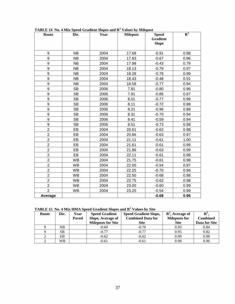
No. 4 Mix
This mix is called a No. 4 mix because the aggregates
pass through the No. 4 sieve, which has a 4.75-mm (0.187-
inch) opening. Therefore, the No. 4 mix is essentially a
4.75-mm Superpave mix. Speed gradients and R2 values are
presented in Tables 15 and 16. Figures 31 through 38
provide scatter plots and linear trend lines for each site,
for both individual mileposts and for entire sites
(mileposts combined). The average speed-gradient slope for
the individual No. 4 mix mileposts was considerably steeper
(-0.68) than for the other mixes, and the R2 value was
indicative of a strong linear association at 0.96. It is
not surprising that the speed-gradient was steeper for this
finer mix, because just as smooth tires are more sensitive
to speed than ribbed tires, smoother (finer) pavements
should be expected to be more sensitive to speed,
especially for a pavement as fine as the No. 4 mix.
The standard deviation of the speed-gradient slopes
between mileposts was +/-0.12. Therefore, the range within
one standard deviation of the mean was -0.56 to -0.80, and
the range within two standard deviations of the mean was
-0.44 to -0.92.
37
TABLE 14 No. 4 Mix Speed Gradient Slopes and R2 Values by Milepost
Route Dir. Year Milepost Speed
Gradient
Slope
R2
9 NB 2004 17.68 -0.91 0.98
9 NB 2004 17.83 -0.67 0.96
9 NB 2004 17.98 -0.43 0.79
9 NB 2004 18.13 -0.79 0.97
9 NB 2004 18.28 -0.78 0.99
9 NB 2004 18.43 -0.48 0.91
9 NB 2004 18.58 -0.77 0.94
9 SB 2006 7.81 -0.80 0.96
9 SB 2006 7.91 -0.85 0.97
9 SB 2006 8.01 -0.77 0.98
9 SB 2006 8.11 -0.72 0.98
9 SB 2006 8.21 -0.96 0.88
9 SB 2006 8.31 -0.70 0.94
9 SB 2006 8.41 -0.59 0.94
9 SB 2006 8.51 -0.73 0.98
2 EB 2004 20.61 -0.62 0.98
2 EB 2004 20.86 -0.63 0.97
2 EB 2004 21.11 -0.61 1.00
2 EB 2004 21.61 -0.61 0.99
2 EB 2004 21.86 -0.63 0.99
2 EB 2004 22.11 -0.61 0.98
2 WB 2004 21.75 -0.61 0.98
2 WB 2004 22.00 -0.54 0.97
2 WB 2004 22.25 -0.70 0.96
2 WB 2004 22.50 -0.68 0.98
2 WB 2004 22.75 -0.62 0.98
2 WB 2004 23.00 -0.60 0.99
2 WB 2004 23.25 -0.54 0.99
Average -0.68 0.96
TABLE 15 No. 4 Mix HMA Speed Gradient Slopes and R2 Values by Site
Route Dir. Year
Paved
Speed Gradient
Slope, Average of
Mileposts for Site
Speed Gradient Slope,
Combined Data for
Site
R2, Average of
Mileposts for
Site
R2,
Combined
Data for Site
9 NB -0.69 -0.70 0.93 0.84
9 SB -0.77 -0.77 0.95 0.82
2 EB -0.62 -0.62 0.99 0.98
2 WB -0.61 -0.61 0.98 0.96
38
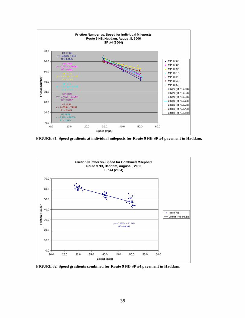
Friction Number vs. Speed for Individual Mileposts
Route 9 NB, Haddam, August 8, 2006
SP #4 (2004)
MP 17.68
y = -0.9056x + 87.8
R2 = 0.9845
MP 17.83
y = -0.6731x + 80.691
R2 = 0.9581
MP 17.98
y = -0.4341x + 74.143
R2 = 0.7945
MP 18.13
y = -0.7924x + 85.444
R2 = 0.9727
MP 18.28
y = -0.7772x + 83.288
R2 = 0.9867
MP 18.43
y = -0.4795x + 74.094
R2 = 0.9061
MP 18.58
y = -0.767x + 86.053
R2 = 0.94340.0
10.0
20.0
30.0
40.0
50.0
60.0
70.0
0.0 10.0 20.0 30.0 40.0 50.0 60.0
Speed (mph)
Fri
cti
on
Nu
mb
er
MP 17.68
MP 17.83
MP 17.98
MP 18.13
MP 18.28
MP 18.43
MP 18.58
Linear (MP 17.68)
Linear (MP 17.83)
Linear (MP 17.98)
Linear (MP 18.13)
Linear (MP 18.28)
Linear (MP 18.43)
Linear (MP 18.58)
FIGURE 31 Speed gradients at individual mileposts for Route 9 NB SP #4 pavement in Haddam.
Friction Number vs. Speed for Combined Mileposts
Route 9 NB, Haddam, August 8, 2006
SP #4 (2004)
y = -0.6955x + 81.865
R2 = 0.8395
0.0
10.0
20.0
30.0
40.0
50.0
60.0
70.0
20.0 25.0 30.0 35.0 40.0 45.0 50.0 55.0 60.0
Speed (mph)
Fri
cti
on
Nu
mb
er
Rte 9 NB
Linear (Rte 9 NB)
FIGURE 32 Speed gradients combined for Route 9 NB SP #4 pavement in Haddam.
39
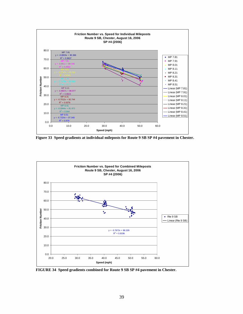
Friction Number vs. Speed for Individual Mileposts
Route 9 SB, Chester, August 16, 2006
SP #4 (2006)
MP 7.81
y = -0.8003x + 90.366
R2 = 0.9637
MP 7.91
y = -0.851x + 89.446
R2 = 0.9683
MP 8.01
y = -0.7745x + 86.366
R2 = 0.9845
MP 8.11
y = -0.7179x + 83.484
R2 = 0.9817
MP 8.21
y = -0.9607x + 88.977
R2 = 0.8823
MP 8.31
y = -0.7012x + 82.744
R2 = 0.9376
MP 8.41
y = -0.5944x + 81.972
R2 = 0.944
MP 8.51
y = -0.7324x + 87.046
R2 = 0.9790.0
10.0
20.0
30.0
40.0
50.0
60.0
70.0
80.0
0.0 10.0 20.0 30.0 40.0 50.0 60.0
Speed (mph)
Fri
cti
on
Nu
mb
er
MP 7.81
MP 7.91
MP 8.01
MP 8.11
MP 8.21
MP 8.31
MP 8.41
MP 8.51
Linear (MP 7.81)
Linear (MP 7.91)
Linear (MP 8.01)
Linear (MP 8.11)
Linear (MP 8.21)
Linear (MP 8.31)
Linear (MP 8.41)
Linear (MP 8.51)
Figure 33 Speed gradients at individual mileposts for Route 9 SB SP #4 pavement in Chester.
Friction Number vs. Speed for Combined Mileposts
Route 9 SB, Chester, August 16, 2006
SP #4 (2006)
y = -0.7672x + 86.326
R2 = 0.8196
0.0
10.0
20.0
30.0
40.0
50.0
60.0
70.0
80.0
20.0 25.0 30.0 35.0 40.0 45.0 50.0 55.0 60.0
Speed (mph)
Fri
cti
on
Nu
mb
er
Rte 9 SB
Linear (Rte 9 SB)
FIGURE 34 Speed gradients combined for Route 9 SB SP #4 pavement in Chester.
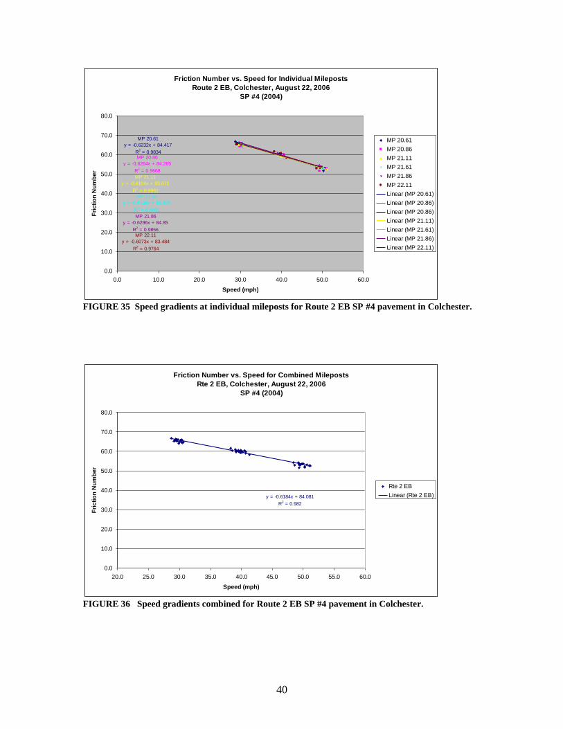
40
Friction Number vs. Speed for Individual Mileposts
Route 2 EB, Colchester, August 22, 2006
SP #4 (2004)
MP 20.61
y = -0.6232x + 84.417
R2 = 0.9834MP 20.86
y = -0.6264x + 84.265
R2 = 0.9668
MP 21.11
y = -0.6104x + 83.671
R2 = 0.9961
MP 21.61
y = -0.6138x + 83.805
R2 = 0.9931
MP 21.86
y = -0.6296x + 84.85
R2 = 0.9856MP 22.11
y = -0.6073x + 83.484
R2 = 0.9764
0.0
10.0
20.0
30.0
40.0
50.0
60.0
70.0
80.0
0.0 10.0 20.0 30.0 40.0 50.0 60.0
Speed (mph)
Fri
cti
on
Nu
mb
er
MP 20.61
MP 20.86
MP 21.11
MP 21.61
MP 21.86
MP 22.11
Linear (MP 20.61)
Linear (MP 20.86)
Linear (MP 20.86)
Linear (MP 21.11)
Linear (MP 21.61)
Linear (MP 21.86)
Linear (MP 22.11)
FIGURE 35 Speed gradients at individual mileposts for Route 2 EB SP #4 pavement in Colchester.
Friction Number vs. Speed for Combined Mileposts
Rte 2 EB, Colchester, August 22, 2006
SP #4 (2004)
y = -0.6184x + 84.081
R2 = 0.982
0.0
10.0
20.0
30.0
40.0
50.0
60.0
70.0
80.0
20.0 25.0 30.0 35.0 40.0 45.0 50.0 55.0 60.0
Speed (mph)
Fri
cti
on
Nu
mb
er
Rte 2 EB
Linear (Rte 2 EB)
FIGURE 36 Speed gradients combined for Route 2 EB SP #4 pavement in Colchester.
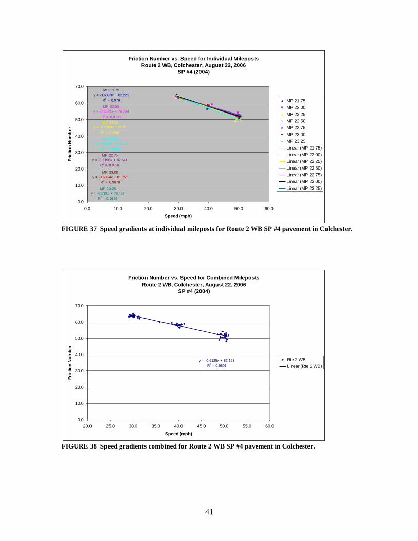
41
Friction Number vs. Speed for Individual Mileposts
Route 2 WB, Colchester, August 22, 2006
SP #4 (2004)
MP 21.75
y = -0.6063x + 82.229
R2 = 0.979
MP 22.00
y = -0.5371x + 79.794
R2 = 0.9738
MP 22.25
y = -0.6984x + 85.01
R2 = 0.9581
MP 22.50
y = -0.6848x + 84.121
R2 = 0.9838
MP 22.75
y = -0.6196x + 82.541
R2 = 0.9791
MP 23.00
y = -0.6004x + 81.755
R2 = 0.9878
MP 23.25
y = -0.539x + 79.457
R2 = 0.98950.0
10.0
20.0
30.0
40.0
50.0
60.0
70.0
0.0 10.0 20.0 30.0 40.0 50.0 60.0
Speed (mph)
Fri
cti
on
Nu
mb
er
MP 21.75
MP 22.00
MP 22.25
MP 22.50
MP 22.75
MP 23.00
MP 23.25
Linear (MP 21.75)
Linear (MP 22.00)
Linear (MP 22.25)
Linear (MP 22.50)
Linear (MP 22.75)
Linear (MP 23.00)
Linear (MP 23.25)
FIGURE 37 Speed gradients at individual mileposts for Route 2 WB SP #4 pavement in Colchester.
Friction Number vs. Speed for Combined Mileposts
Route 2 WB, Colchester, August 22, 2006
SP #4 (2004)
y = -0.6125x + 82.153
R2 = 0.9591
0.0
10.0
20.0
30.0
40.0
50.0
60.0
70.0
20.0 25.0 30.0 35.0 40.0 45.0 50.0 55.0 60.0
Speed (mph)
Fri
cti
on
Nu
mb
er
Rte 2 WB
Linear (Rte 2 WB)
FIGURE 38 Speed gradients combined for Route 2 WB SP #4 pavement in Colchester.
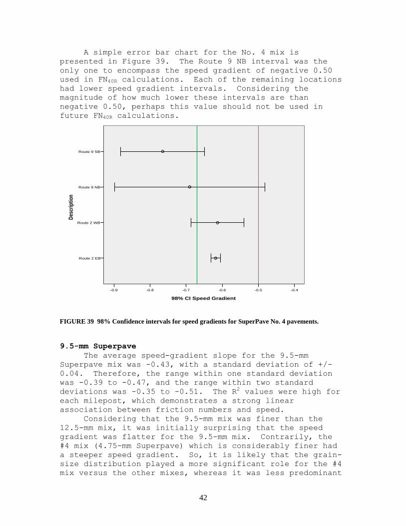
42
A simple error bar chart for the No. 4 mix is
presented in Figure 39. The Route 9 NB interval was the
only one to encompass the speed gradient of negative 0.50
used in FN40R calculations. Each of the remaining locations
had lower speed gradient intervals. Considering the
magnitude of how much lower these intervals are than
negative 0.50, perhaps this value should not be used in
future FN40R calculations.
Route 9 SB
Route 9 NB
Route 2 WB
Route 2 EB
Des
crip
tio
n
-0.4-0.5-0.6-0.7-0.8-0.9
98% CI Speed Gradient
FIGURE 39 98% Confidence intervals for speed gradients for SuperPave No. 4 pavements.
9.5-mm Superpave
The average speed-gradient slope for the 9.5-mm
Superpave mix was -0.43, with a standard deviation of +/-
0.04. Therefore, the range within one standard deviation
was -0.39 to -0.47, and the range within two standard
deviations was -0.35 to -0.51. The R2 values were high for
each milepost, which demonstrates a strong linear
association between friction numbers and speed.
Considering that the 9.5-mm mix was finer than the
12.5-mm mix, it was initially surprising that the speed
gradient was flatter for the 9.5-mm mix. Contrarily, the
#4 mix (4.75-mm Superpave) which is considerably finer had
a steeper speed gradient. So, it is likely that the grain-
size distribution played a more significant role for the #4
mix versus the other mixes, whereas it was less predominant
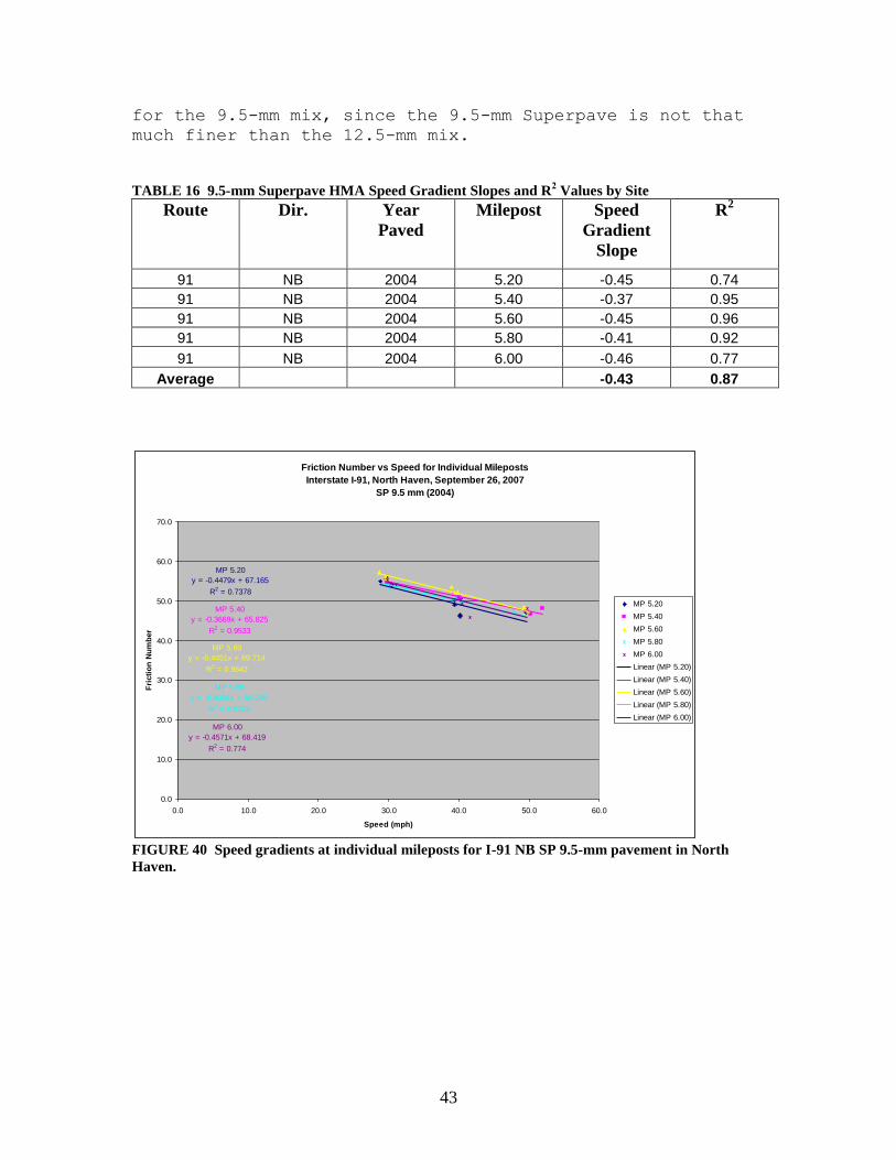
43
for the 9.5-mm mix, since the 9.5-mm Superpave is not that
much finer than the 12.5-mm mix.
TABLE 16 9.5-mm Superpave HMA Speed Gradient Slopes and R2 Values by Site
Route Dir. Year
Paved
Milepost Speed
Gradient
Slope
R2
91 NB 2004 5.20 -0.45 0.74
91 NB 2004 5.40 -0.37 0.95
91 NB 2004 5.60 -0.45 0.96
91 NB 2004 5.80 -0.41 0.92
91 NB 2004 6.00 -0.46 0.77
Average -0.43 0.87
Friction Number vs Speed for Individual Mileposts
Interstate I-91, North Haven, September 26, 2007
SP 9.5 mm (2004)
MP 5.20
y = -0.4479x + 67.165
R2 = 0.7378
MP 5.40
y = -0.3669x + 65.825
R2 = 0.9533
MP 5.60
y = -0.4451x + 69.714
R2 = 0.9642
MP 5.80
y = -0.4084x + 66.286
R2 = 0.9223
MP 6.00
y = -0.4571x + 68.419
R2 = 0.774
0.0
10.0
20.0
30.0
40.0
50.0
60.0
70.0
0.0 10.0 20.0 30.0 40.0 50.0 60.0
Speed (mph)
Fri
cti
on
Nu
mb
er
MP 5.20
MP 5.40
MP 5.60
MP 5.80
MP 6.00
Linear (MP 5.20)
Linear (MP 5.40)
Linear (MP 5.60)
Linear (MP 5.80)
Linear (MP 6.00)
FIGURE 40 Speed gradients at individual mileposts for I-91 NB SP 9.5-mm pavement in North
Haven.
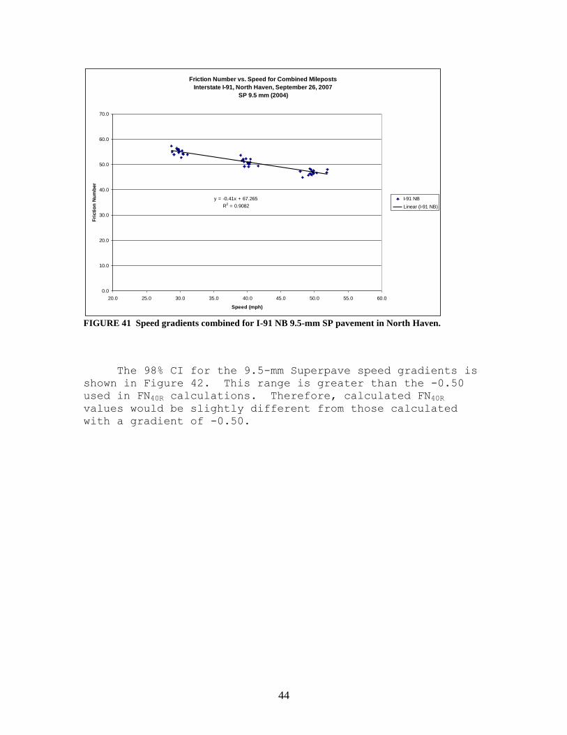
44
Friction Number vs. Speed for Combined Mileposts
Interstate I-91, North Haven, September 26, 2007
SP 9.5 mm (2004)
y = -0.41x + 67.265
R2 = 0.9082
0.0
10.0
20.0
30.0
40.0
50.0
60.0
70.0
20.0 25.0 30.0 35.0 40.0 45.0 50.0 55.0 60.0
Speed (mph)
Fri
cti
on
Nu
mb
er
I-91 NB
Linear (I-91 NB)
FIGURE 41 Speed gradients combined for I-91 NB 9.5-mm SP pavement in North Haven.
The 98% CI for the 9.5-mm Superpave speed gradients is
shown in Figure 42. This range is greater than the -0.50
used in FN40R calculations. Therefore, calculated FN40R
values would be slightly different from those calculated
with a gradient of -0.50.
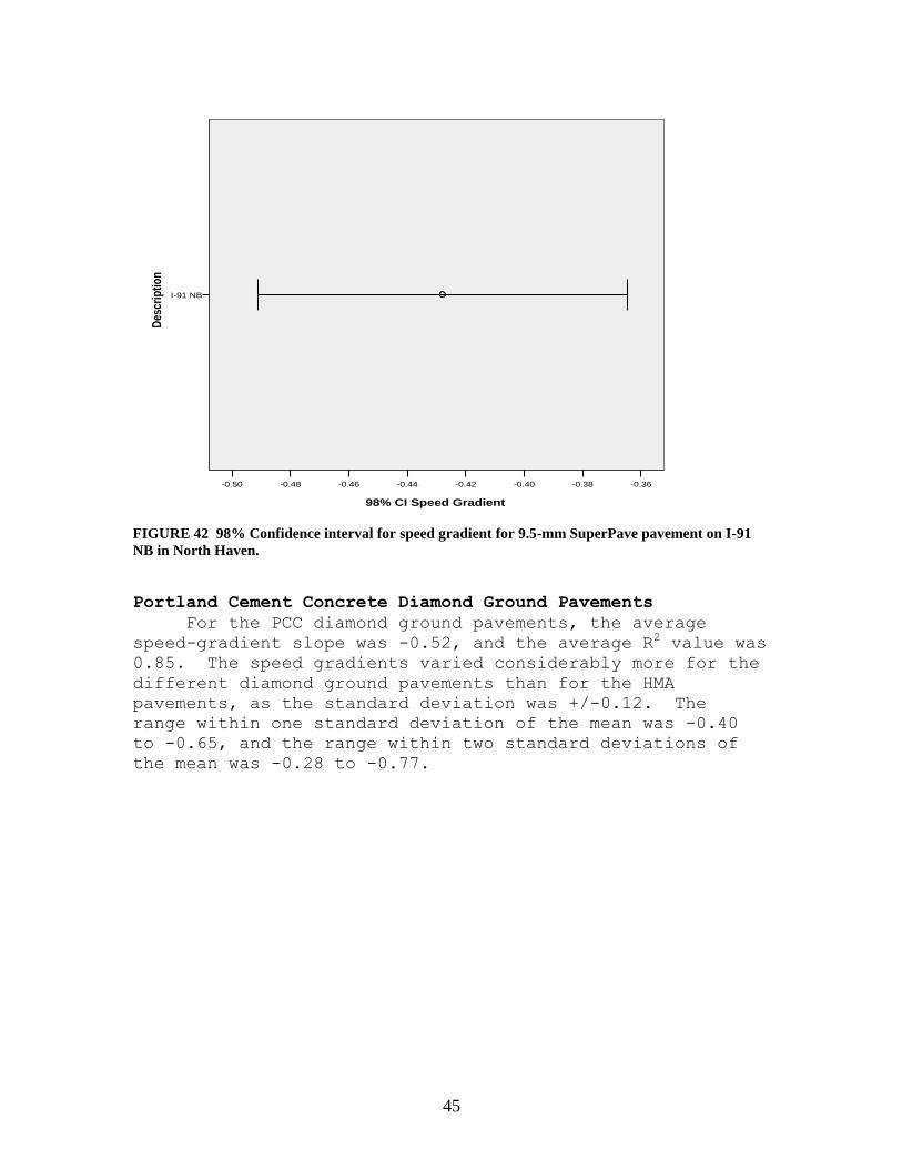
45
I-91 NB
Des
crip
tio
n
-0.36-0.38-0.40-0.42-0.44-0.46-0.48-0.50
98% CI Speed Gradient
FIGURE 42 98% Confidence interval for speed gradient for 9.5-mm SuperPave pavement on I-91
NB in North Haven.
Portland Cement Concrete Diamond Ground Pavements
For the PCC diamond ground pavements, the average
speed-gradient slope was -0.52, and the average R2 value was
0.85. The speed gradients varied considerably more for the
different diamond ground pavements than for the HMA
pavements, as the standard deviation was +/-0.12. The
range within one standard deviation of the mean was -0.40
to -0.65, and the range within two standard deviations of
the mean was -0.28 to -0.77.
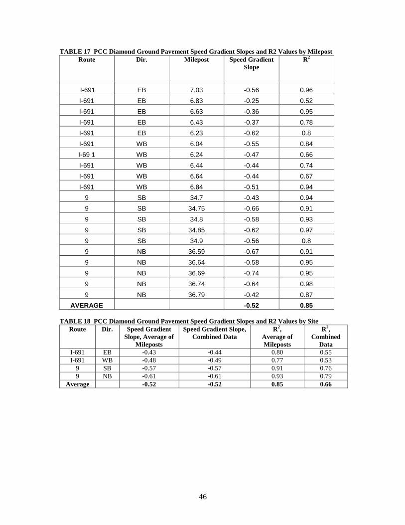
46
TABLE 17 PCC Diamond Ground Pavement Speed Gradient Slopes and R2 Values by Milepost
Route Dir. Milepost Speed Gradient
Slope
R2
I-691 EB 7.03 -0.56 0.96
I-691 EB 6.83 -0.25 0.52
I-691 EB 6.63 -0.36 0.95
I-691 EB 6.43 -0.37 0.78
I-691 EB 6.23 -0.62 0.8
I-691 WB 6.04 -0.55 0.84
I-69 1 WB 6.24 -0.47 0.66
I-691 WB 6.44 -0.44 0.74
I-691 WB 6.64 -0.44 0.67
I-691 WB 6.84 -0.51 0.94
9 SB 34.7 -0.43 0.94
9 SB 34.75 -0.66 0.91
9 SB 34.8 -0.58 0.93
9 SB 34.85 -0.62 0.97
9 SB 34.9 -0.56 0.8
9 NB 36.59 -0.67 0.91
9 NB 36.64 -0.58 0.95
9 NB 36.69 -0.74 0.95
9 NB 36.74 -0.64 0.98
9 NB 36.79 -0.42 0.87
AVERAGE -0.52 0.85
TABLE 18 PCC Diamond Ground Pavement Speed Gradient Slopes and R2 Values by Site
Route Dir. Speed Gradient
Slope, Average of
Mileposts
Speed Gradient Slope,
Combined Data
R2,
Average of
Mileposts
R2,
Combined
Data
I-691 EB -0.43 -0.44 0.80 0.55
I-691 WB -0.48 -0.49 0.77 0.53
9 SB -0.57 -0.57 0.91 0.76
9 NB -0.61 -0.61 0.93 0.79
Average -0.52 -0.52 0.85 0.66
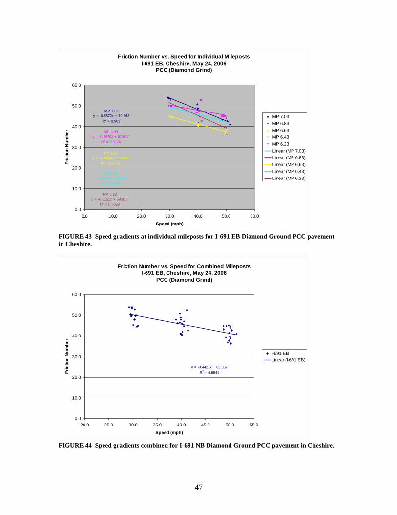
47
Friction Number vs. Speed for Individual Mileposts
I-691 EB, Cheshire, May 24, 2006
PCC (Diamond Grind)
MP 7.03
y = -0.5572x + 70.562
R2 = 0.963
MP 6.83
y = -0.2476x + 57.677
R2 = 0.5174
MP 6.63
y = -0.3629x + 55.663
R2 = 0.9497
MP 6.43
y = -0.3724x + 60.631
R2 = 0.7834
MP 6.23
y = -0.6151x + 69.818
R2 = 0.8029
0.0
10.0
20.0
30.0
40.0
50.0
60.0
0.0 10.0 20.0 30.0 40.0 50.0 60.0
Speed (mph)
Fri
cti
on
Nu
mb
er
MP 7.03
MP 6.83
MP 6.63
MP 6.43
MP 6.23
Linear (MP 7.03)
Linear (MP 6.83)
Linear (MP 6.63)
Linear (MP 6.43)
Linear (MP 6.23)
FIGURE 43 Speed gradients at individual mileposts for I-691 EB Diamond Ground PCC pavement
in Cheshire.
Friction Number vs. Speed for Combined Mileposts
I-691 EB, Cheshire, May 24, 2006
PCC (Diamond Grind)
y = -0.4421x + 63.307
R2 = 0.5541
0.0
10.0
20.0
30.0
40.0
50.0
60.0
20.0 25.0 30.0 35.0 40.0 45.0 50.0 55.0
Speed (mph)
Fri
cti
on
Nu
mb
er
I-691 EB
Linear (I-691 EB)
FIGURE 44 Speed gradients combined for I-691 NB Diamond Ground PCC pavement in Cheshire.
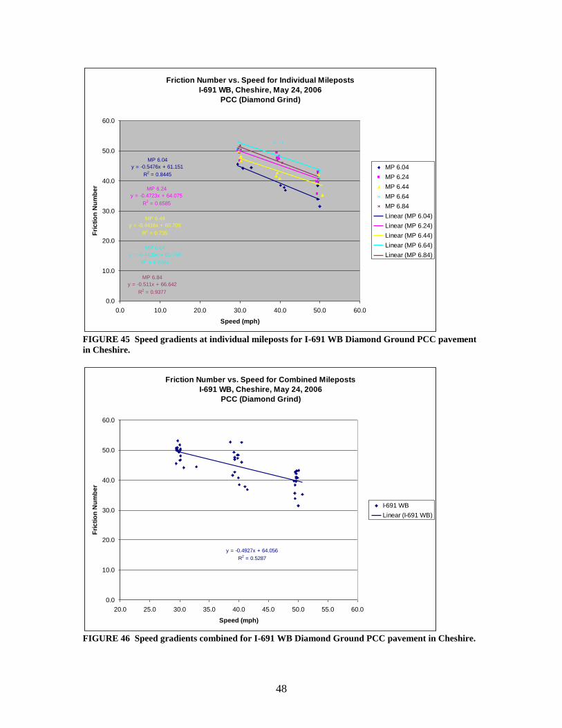
48
Friction Number vs. Speed for Individual Mileposts
I-691 WB, Cheshire, May 24, 2006
PCC (Diamond Grind)
MP 6.04
y = -0.5476x + 61.151
R2 = 0.8445
MP 6.24
y = -0.4723x + 64.075
R2 = 0.6585
MP 6.44
y = -0.4416x + 60.709
R2 = 0.735
MP 6.64
y = -0.4405x + 65.744
R2 = 0.6684
MP 6.84
y = -0.511x + 66.642
R2 = 0.9377
0.0
10.0
20.0
30.0
40.0
50.0
60.0
0.0 10.0 20.0 30.0 40.0 50.0 60.0
Speed (mph)
Fri
cti
on
Nu
mb
er
MP 6.04
MP 6.24
MP 6.44
MP 6.64
MP 6.84
Linear (MP 6.04)
Linear (MP 6.24)
Linear (MP 6.44)
Linear (MP 6.64)
Linear (MP 6.84)
FIGURE 45 Speed gradients at individual mileposts for I-691 WB Diamond Ground PCC pavement
in Cheshire.
Friction Number vs. Speed for Combined Mileposts
I-691 WB, Cheshire, May 24, 2006
PCC (Diamond Grind)
y = -0.4927x + 64.056
R2 = 0.5287
0.0
10.0
20.0
30.0
40.0
50.0
60.0
20.0 25.0 30.0 35.0 40.0 45.0 50.0 55.0 60.0
Speed (mph)
Fri
cti
on
Nu
mb
er
I-691 WB
Linear (I-691 WB)
FIGURE 46 Speed gradients combined for I-691 WB Diamond Ground PCC pavement in Cheshire.
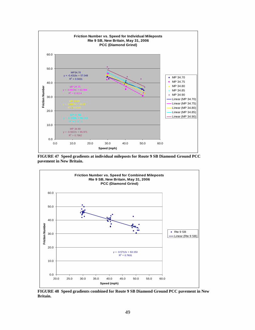
49
Friction Number vs. Speed for Individual Mileposts
Rte 9 SB, New Britain, May 31, 2006
PCC (Diamond Grind)
MP34.70
y = -0.4316x + 57.048
R2 = 0.9431
MP 34.75
y = -0.6624x + 63.984
R2 = 0.9114
MP 34.80
y = -0.5805x + 62.87
R2 = 0.9336
MP 34.85
y = -0.6228x + 66.019
R2 = 0.9713
MP 34.90
y = -0.5622x + 65.971
R2 = 0.7962
0.0
10.0
20.0
30.0
40.0
50.0
60.0
0.0 10.0 20.0 30.0 40.0 50.0 60.0
Speed (mph)
Fri
cti
on
Nu
mb
er
MP 34.70
MP 34.75
MP 34.80
MP 34.85
MP 34.90
Linear (MP 34.70)
Linear (MP 34.75)
Linear (MP 34.80)
Linear (MP 34.85)
Linear (MP 34.90)
FIGURE 47 Speed gradients at individual mileposts for Route 9 SB Diamond Ground PCC
pavement in New Britain.
Friction Number vs. Speed for Combined Mileposts
Rte 9 SB, New Britain, May 31, 2006
PCC (Diamond Grind)
y = -0.5712x + 63.153
R2 = 0.7631
0.0
10.0
20.0
30.0
40.0
50.0
60.0
20.0 25.0 30.0 35.0 40.0 45.0 50.0 55.0 60.0
Speed (mph)
Fri
cti
on
Nu
mb
er
Rte 9 SB
Linear (Rte 9 SB)
FIGURE 48 Speed gradients combined for Route 9 SB Diamond Ground PCC pavement in New
Britain.
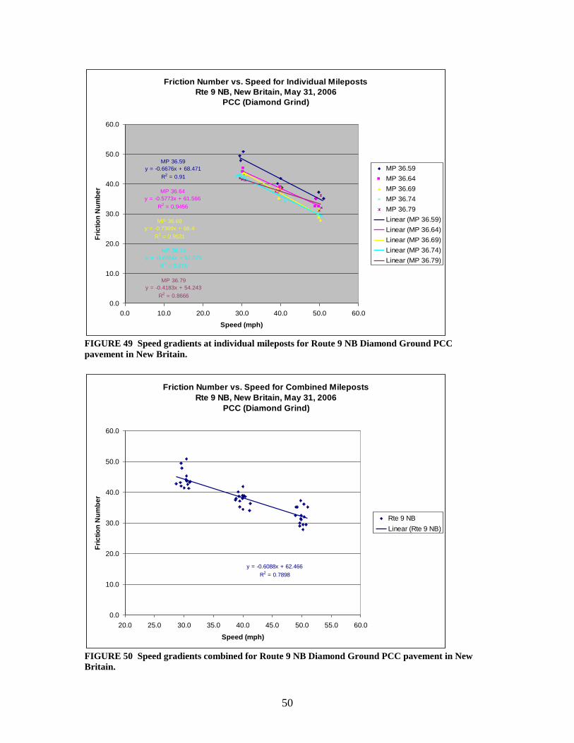
50
Friction Number vs. Speed for Individual Mileposts
Rte 9 NB, New Britain, May 31, 2006
PCC (Diamond Grind)
MP 36.59
y = -0.6676x + 68.471
R2 = 0.91
MP 36.64
y = -0.5773x + 61.566
R2 = 0.9456
MP 36.69
y = -0.7369x + 66.4
R2 = 0.9531
MP 36.74
y = -0.6364x + 61.376
R2 = 0.976
MP 36.79
y = -0.4183x + 54.243
R2 = 0.8666
0.0
10.0
20.0
30.0
40.0
50.0
60.0
0.0 10.0 20.0 30.0 40.0 50.0 60.0
Speed (mph)
Fri
cti
on
Nu
mb
er
MP 36.59
MP 36.64
MP 36.69
MP 36.74
MP 36.79
Linear (MP 36.59)
Linear (MP 36.64)
Linear (MP 36.69)
Linear (MP 36.74)
Linear (MP 36.79)
FIGURE 49 Speed gradients at individual mileposts for Route 9 NB Diamond Ground PCC
pavement in New Britain.
Friction Number vs. Speed for Combined Mileposts
Rte 9 NB, New Britain, May 31, 2006
PCC (Diamond Grind)
y = -0.6088x + 62.466
R2 = 0.7898
0.0
10.0
20.0
30.0
40.0
50.0
60.0
20.0 25.0 30.0 35.0 40.0 45.0 50.0 55.0 60.0
Speed (mph)
Fri
cti
on
Nu
mb
er
Rte 9 NB
Linear (Rte 9 NB)
FIGURE 50 Speed gradients combined for Route 9 NB Diamond Ground PCC pavement in New
Britain.
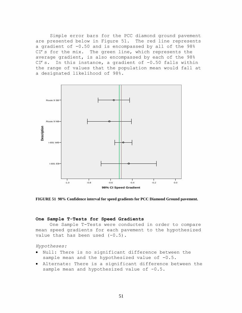
51
Simple error bars for the PCC diamond ground pavement
are presented below in Figure 51. The red line represents
a gradient of -0.50 and is encompassed by all of the 98%
CI’s for the mix. The green line, which represents the
average gradient, is also encompassed by each of the 98%
CI’s. In this instance, a gradient of -0.50 falls within
the range of values that the population mean would fall at
a designated likelihood of 98%.
Route 9 SB
Route 9 NB
I-691 WB
I-691 EB
Des
crip
tio
n
0.0-0.2-0.4-0.6-0.8-1.0
98% CI Speed Gradient
FIGURE 51 98% Confidence interval for speed gradients for PCC Diamond Ground pavement.
One Sample T-Tests for Speed Gradients
One Sample T-Tests were conducted in order to compare
mean speed gradients for each pavement to the hypothesized
value that has been used (-0.5).
Hypotheses:
Null: There is no significant difference between the
sample mean and the hypothesized value of -0.5.
Alternate: There is a significant difference between the
sample mean and hypothesized value of -0.5.

52
TABLE 19 One-Sample Statistics for Speed Gradients
N Mean Std. Deviation Std. Error Mean
Class 1 Pavement 27 -.4041 .09221 .01775
SP 12 mm Pavement 25 -.5032 .10303 .02061
No. 4 Mix Pavement 28 -.6768 .12257 .02316
PCC Pavement 20 .5235 .12364 .02765
SP 9.5 mm Pavement 5 -.4280 .03768 .01685
TABLE 20 One-Sample Tests for Speed Gradients
Test Value = -0.5
t df Sig. (2-tailed) Mean
Difference 95% Confidence Interval of
the Difference
Lower Upper
Class 1 Pavement 5.406 26 1.155E-005 .09593 .0595 .1324
SP 12.5 mm Pavement -.155 24 .8779 -.00320 -.0457 .0393
No. 4 Mix Pavement -7.632 27 3.290E-008 -.17679 -.2243 -.1293
PCC Pavement 37.02 19 3.553E-019 1.02350 .9656 1.0814
SP 9.5 mm Pavement 4.272 4 .0129 .07200 .0252 .1188
For the Class 1 HMA, the mean value was -0.40, which
differed by 0.1 from the hypothesized value of -0.5. The
results of the One Sample T-Test calculated a t value of
5.406 and 26 degrees of freedom. The significance value
was only 1.155E-005, which is considerably less than the
chosen significance level of 0.05. Note: the significance
level is the probability of rejecting the null hypothesis
when it is true. Therefore, the sample mean of -0.40 is
significantly different than -0.50. The null hypothesis is
rejected for the Class 1 HMA samples.
The null hypothesis was also rejected for the No. 4
and 9.5-mm Superpave HMA mixes, and for the PCC pavement.
For the 12.5-mm Superpave HMA, the value is -0.50.
This is very close to the hypothesized value. The results
of the One Sample T-test show a t value of -0.155 and 24
degrees of freedom. The significance value is 0.88, which
is greater than 0.05. Therefore, the test failed to reject
the null hypothesis for the 12.5-mm Superpave HMA.
Discussion
A research objective was to update friction number
speed correction factors for FN40R calculations based upon
the various pavement mix designs used in Connecticut.
Currently, ConnDOT uses a speed correction factor of -0.5
53
for all pavements. This factor is used in the following
equation:
FN40R = FN – 0.5 * (40 – speed)
where,
FN40R = friction number with a standard Ribbed Tire
based upon a corrected speed o 40 mph,
FN = measured friction number, and
speed = measured speed in mph.
One Sample T-tests demonstrated significant
differences between sample speed gradient means and the
hypothesized value of -0.5 for the ConnDOT Class 1, 9.5-mm
Superpave, and No. 4 HMAs. Conversely, the T-Test failed
to reject the null hypothesis for the 12.5-mm Superpave
HMA. This implies that the data were not sufficiently
persuasive to indicate a significant difference exists
between the sample mean 12.5-mm speed gradient and the
hypothesized value of -0.5.
Finer mixes, such as the #4 mix (4.75-mm
Superpave), appear to be most problematic. The average #4
mix speed gradient was significantly less than -0.5
(-0.68). This is because finer mixes result in less open-
graded surfaces. The author’s theory is that these dense-
surfaced mixes behave similarly to smooth tires insofar as
the tire-pavement interface is concerned, and just as
smooth tires have steeper speed gradients, so do smooth
pavements. In fact, a smooth-tire speed gradient of nearly
-1.0 was measured from the ConnDOT friction tester at the
Virginia Smart Road at an equipment rodeo and reported in a
paper by de Leon et al (15). A smooth-surfaced pavement
likely results in a steep gradient.
CONNDOT’S PRELIMINARY EVALUATION OF THE INTERNATIONAL
FRICTION INDEX COEFFICIENTS
Since ConnDOT personnel can now measure pavement
texture with either the CTMeter or with the high-speed
laser device mounted to the friction tester, they have the
ability to calculate the IFI of pavement surfaces on
Connecticut roadways.
The practice of calculating the IFI of a pavement is
performed in accordance with ASTM 1960. The specification
54
states “The IFI was developed in the PIARC [Permanent
International Association of Road Congresses] International
experiment to Compare and Harmonize Texture and Skid
Resistance Measurements.” It also states the IFI provides
a way of harmonizing pavement friction measured with
different equipment to a common calibrated index, and for
harmonizing friction measured with a smooth test tire.
Two parameters are calculated in the practice: the
calibrated wet friction at 60 km/h (F60) and the speed
constant of wet pavement friction (Sp). Sp is sometimes
referred to as the speed gradient. The equation for
calculating the speed gradient is:
Sp = 14.2 + 89.7 MPD. (1)
Before F60 can be calculated, the measured friction
(FRS) at some slip speed (S) is used with Sp to calculate
the friction at 60 km/h (FR60). The equation for
calculating FR60 is:
FR60 = FRS x EXP[(S-60)/ Sp]. (2)
Finally, two calibration constants (A,B) are used with FR60
to calculate F60 as follows:
F60 = A + B x FR60. (3)
The problem that was encountered in using equation (3)
above was that A and B are determined from a linear
regression of the values of FR60 calculated with yet
another equation which requires a Dynamic Friction Tester
(DFTester) number measured with a device called the Dynamic
Friction Tester, which ConnDOT does not own:
FR60 = 0.081 + 0.732(DFT20)(EXP(-40/ Sp)) (4)
where
DFT20 is the Dynamic Friction Tester number at 20 km/h
measured in accordance with ASTM E 1911 for a “set of at
least 10 different pavements having a range of macrotexture
and microtexture.”
The previous ASTM E 1960 standard from 1998 (E 1960-
98), provided the calibration constants (A,B,C) in an
appendix. Since ConnDOT does not currently own a Dynamic
Friction Tester (DFTester), the constants from the 1998
55
version of ASTM E 1960-98 had to be used for this research
in order to calculate the IFI coefficient F60. The 1998
equation was:
F60 = A + B x FR60 + C x MPD (5)
Equations (1), (2), and (5) were used to calculate the
IFI parameters Sp and F60, presented as IFI(F60,Sp), for the
24 pavement sections at the Smart Roads facility in
Virginia. Table 20 below presents the results calculated
with both the CTMeter and the high-speed laser. Sp values
calculated with the CTMeter MPDs ranged from 61 to 186
km/h, and F60 values ranged from 0.399 to 0.589. Sp values
calculated with the high-speed laser MPDs ranged from 55 to
169 km/h, and F60 values ranged from .405 to .481.
The two sets of F60 values described above did not
correlate well to one another, as the R2 value was only
0.28. When the Cargill sections were excluded from the
dataset, as they were for comparing MPD values in Report 2
of this study (16), the R2 value improved only slightly to
0.36. Since Sp values were calculated with a linear
equation (equation (1)), they corresponded to one another
exactly as the MPD values that were used to calculate them.
The coefficient of determination comparing all of the Sp
values was only 0.20, but when the Cargill sections were
excluded, the R2 value increased to 0.61. Since the Cargill
section does not compare to anything used in Connecticut at
this time, excluding the Cargill section is reasonable.
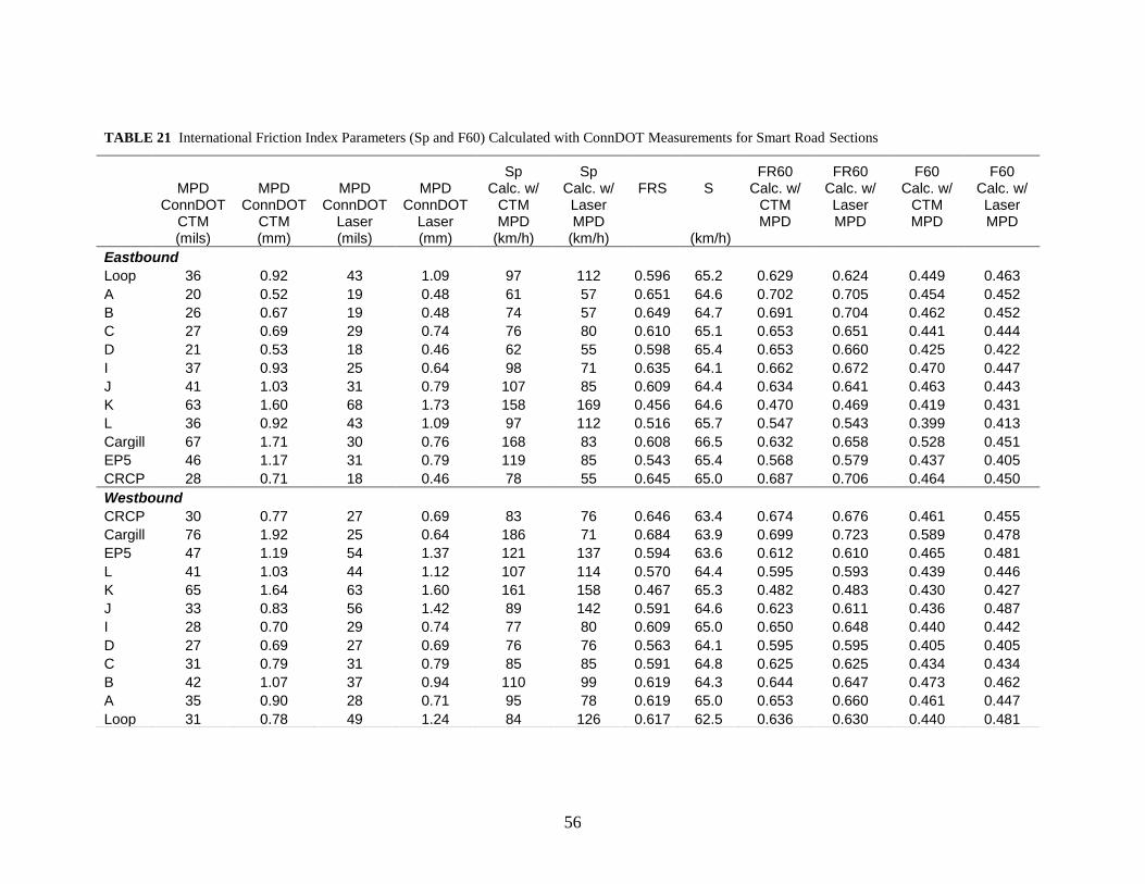
56
TABLE 21 International Friction Index Parameters (Sp and F60) Calculated with ConnDOT Measurements for Smart Road Sections
Sp Calc. w/
CTM MPD
(km/h)
Sp Calc. w/ Laser MPD
(km/h)
FRS
S (km/h)
FR60 FR60 F60 F60
MPD ConnDOT
CTM (mils)
MPD ConnDOT
CTM (mm)
MPD ConnDOT
Laser (mils)
MPD ConnDOT
Laser (mm)
Calc. w/ CTM MPD
Calc. w/ Laser MPD
Calc. w/ CTM MPD
Calc. w/ Laser MPD
Eastbound
Loop 36 0.92 43 1.09 97 112 0.596 65.2 0.629 0.624 0.449 0.463
A 20 0.52 19 0.48 61 57 0.651 64.6 0.702 0.705 0.454 0.452
B 26 0.67 19 0.48 74 57 0.649 64.7 0.691 0.704 0.462 0.452
C 27 0.69 29 0.74 76 80 0.610 65.1 0.653 0.651 0.441 0.444
D 21 0.53 18 0.46 62 55 0.598 65.4 0.653 0.660 0.425 0.422
I 37 0.93 25 0.64 98 71 0.635 64.1 0.662 0.672 0.470 0.447
J 41 1.03 31 0.79 107 85 0.609 64.4 0.634 0.641 0.463 0.443
K 63 1.60 68 1.73 158 169 0.456 64.6 0.470 0.469 0.419 0.431
L 36 0.92 43 1.09 97 112 0.516 65.7 0.547 0.543 0.399 0.413
Cargill 67 1.71 30 0.76 168 83 0.608 66.5 0.632 0.658 0.528 0.451
EP5 46 1.17 31 0.79 119 85 0.543 65.4 0.568 0.579 0.437 0.405
CRCP 28 0.71 18 0.46 78 55 0.645 65.0 0.687 0.706 0.464 0.450
Westbound
CRCP 30 0.77 27 0.69 83 76 0.646 63.4 0.674 0.676 0.461 0.455
Cargill 76 1.92 25 0.64 186 71 0.684 63.9 0.699 0.723 0.589 0.478
EP5 47 1.19 54 1.37 121 137 0.594 63.6 0.612 0.610 0.465 0.481
L 41 1.03 44 1.12 107 114 0.570 64.4 0.595 0.593 0.439 0.446
K 65 1.64 63 1.60 161 158 0.467 65.3 0.482 0.483 0.430 0.427
J 33 0.83 56 1.42 89 142 0.591 64.6 0.623 0.611 0.436 0.487
I 28 0.70 29 0.74 77 80 0.609 65.0 0.650 0.648 0.440 0.442
D 27 0.69 27 0.69 76 76 0.563 64.1 0.595 0.595 0.405 0.405
C 31 0.79 31 0.79 85 85 0.591 64.8 0.625 0.625 0.434 0.434
B 42 1.07 37 0.94 110 99 0.619 64.3 0.644 0.647 0.473 0.462
A 35 0.90 28 0.71 95 78 0.619 65.0 0.653 0.660 0.461 0.447
Loop 31 0.78 49 1.24 84 126 0.617 62.5 0.636 0.630 0.440 0.481
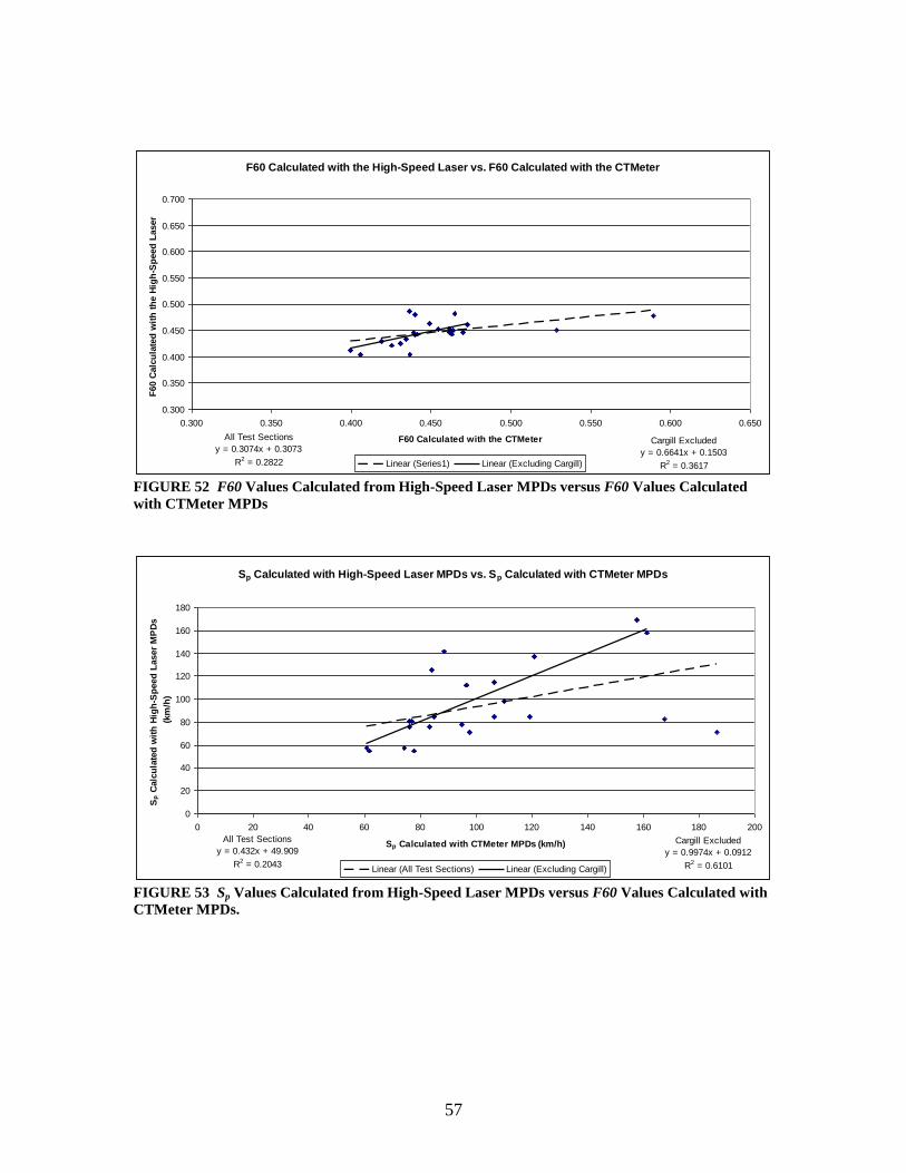
57
F60 Calculated with the High-Speed Laser vs. F60 Calculated with the CTMeter
All Test Sections
y = 0.3074x + 0.3073
R2 = 0.2822
Cargill Excluded
y = 0.6641x + 0.1503
R2 = 0.3617
0.300
0.350
0.400
0.450
0.500
0.550
0.600
0.650
0.700
0.300 0.350 0.400 0.450 0.500 0.550 0.600 0.650
F60 Calculated with the CTMeter
F60 C
alc
ula
ted
wit
h t
he H
igh
-Sp
eed
Laser
Linear (Series1) Linear (Excluding Cargill)
FIGURE 52 F60 Values Calculated from High-Speed Laser MPDs versus F60 Values Calculated
with CTMeter MPDs
Sp Calculated with High-Speed Laser MPDs vs. Sp Calculated with CTMeter MPDs
All Test Sections
y = 0.432x + 49.909
R2 = 0.2043
Cargill Excluded
y = 0.9974x + 0.0912
R2 = 0.6101
0
20
40
60
80
100
120
140
160
180
0 20 40 60 80 100 120 140 160 180 200
Sp Calculated with CTMeter MPDs (km/h)
Sp C
alc
ula
ted
wit
h H
igh
-Sp
eed
Laser
MP
Ds
(km
/h)
Linear (All Test Sections) Linear (Excluding Cargill)
FIGURE 53 Sp Values Calculated from High-Speed Laser MPDs versus F60 Values Calculated with
CTMeter MPDs.
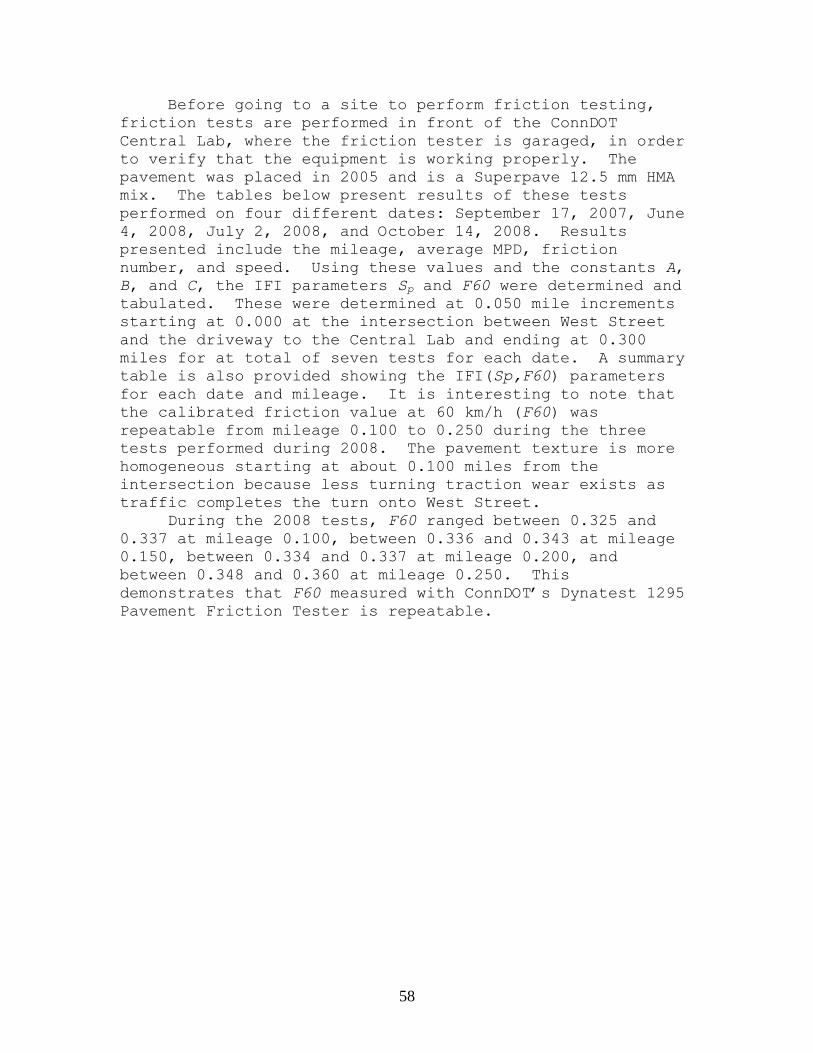
58
Before going to a site to perform friction testing,
friction tests are performed in front of the ConnDOT
Central Lab, where the friction tester is garaged, in order
to verify that the equipment is working properly. The
pavement was placed in 2005 and is a Superpave 12.5 mm HMA
mix. The tables below present results of these tests
performed on four different dates: September 17, 2007, June
4, 2008, July 2, 2008, and October 14, 2008. Results
presented include the mileage, average MPD, friction
number, and speed. Using these values and the constants A,
B, and C, the IFI parameters Sp and F60 were determined and
tabulated. These were determined at 0.050 mile increments
starting at 0.000 at the intersection between West Street
and the driveway to the Central Lab and ending at 0.300
miles for at total of seven tests for each date. A summary
table is also provided showing the IFI(Sp,F60) parameters
for each date and mileage. It is interesting to note that
the calibrated friction value at 60 km/h (F60) was
repeatable from mileage 0.100 to 0.250 during the three
tests performed during 2008. The pavement texture is more
homogeneous starting at about 0.100 miles from the
intersection because less turning traction wear exists as
traffic completes the turn onto West Street.
During the 2008 tests, F60 ranged between 0.325 and
0.337 at mileage 0.100, between 0.336 and 0.343 at mileage
0.150, between 0.334 and 0.337 at mileage 0.200, and
between 0.348 and 0.360 at mileage 0.250. This
demonstrates that F60 measured with ConnDOT’s Dynatest 1295
Pavement Friction Tester is repeatable.
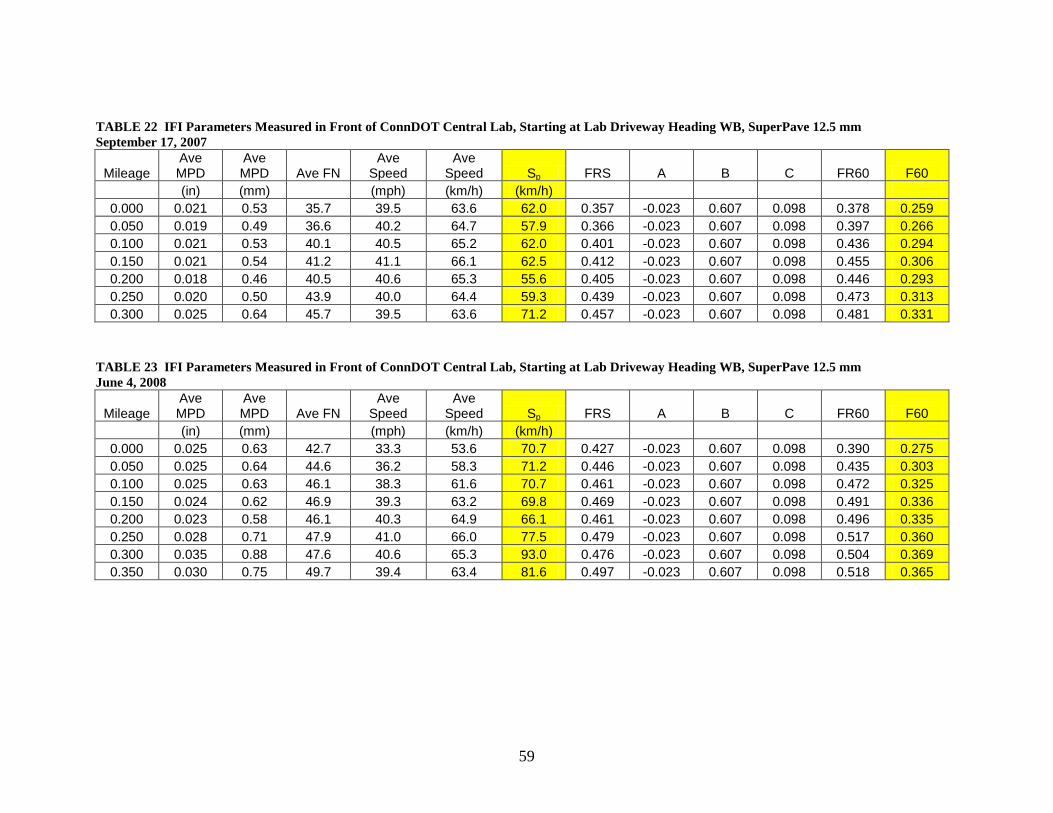
59
TABLE 22 IFI Parameters Measured in Front of ConnDOT Central Lab, Starting at Lab Driveway Heading WB, SuperPave 12.5 mm
September 17, 2007
Mileage Ave MPD
Ave MPD Ave FN
Ave Speed
Ave Speed Sp FRS A B C FR60 F60
(in) (mm) (mph) (km/h) (km/h)
0.000 0.021 0.53 35.7 39.5 63.6 62.0 0.357 -0.023 0.607 0.098 0.378 0.259
0.050 0.019 0.49 36.6 40.2 64.7 57.9 0.366 -0.023 0.607 0.098 0.397 0.266
0.100 0.021 0.53 40.1 40.5 65.2 62.0 0.401 -0.023 0.607 0.098 0.436 0.294
0.150 0.021 0.54 41.2 41.1 66.1 62.5 0.412 -0.023 0.607 0.098 0.455 0.306
0.200 0.018 0.46 40.5 40.6 65.3 55.6 0.405 -0.023 0.607 0.098 0.446 0.293
0.250 0.020 0.50 43.9 40.0 64.4 59.3 0.439 -0.023 0.607 0.098 0.473 0.313
0.300 0.025 0.64 45.7 39.5 63.6 71.2 0.457 -0.023 0.607 0.098 0.481 0.331
TABLE 23 IFI Parameters Measured in Front of ConnDOT Central Lab, Starting at Lab Driveway Heading WB, SuperPave 12.5 mm
June 4, 2008
Mileage Ave MPD
Ave MPD Ave FN
Ave Speed
Ave Speed Sp FRS A B C FR60 F60
(in) (mm) (mph) (km/h) (km/h)
0.000 0.025 0.63 42.7 33.3 53.6 70.7 0.427 -0.023 0.607 0.098 0.390 0.275
0.050 0.025 0.64 44.6 36.2 58.3 71.2 0.446 -0.023 0.607 0.098 0.435 0.303
0.100 0.025 0.63 46.1 38.3 61.6 70.7 0.461 -0.023 0.607 0.098 0.472 0.325
0.150 0.024 0.62 46.9 39.3 63.2 69.8 0.469 -0.023 0.607 0.098 0.491 0.336
0.200 0.023 0.58 46.1 40.3 64.9 66.1 0.461 -0.023 0.607 0.098 0.496 0.335
0.250 0.028 0.71 47.9 41.0 66.0 77.5 0.479 -0.023 0.607 0.098 0.517 0.360
0.300 0.035 0.88 47.6 40.6 65.3 93.0 0.476 -0.023 0.607 0.098 0.504 0.369
0.350 0.030 0.75 49.7 39.4 63.4 81.6 0.497 -0.023 0.607 0.098 0.518 0.365
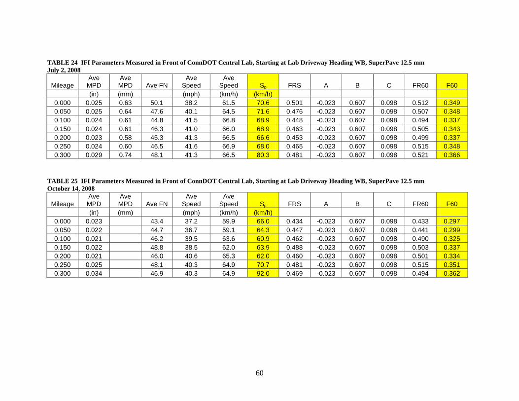
60
TABLE 24 IFI Parameters Measured in Front of ConnDOT Central Lab, Starting at Lab Driveway Heading WB, SuperPave 12.5 mm
July 2, 2008
Mileage Ave MPD
Ave MPD Ave FN
Ave Speed
Ave Speed Sp FRS A B C FR60 F60
(in) (mm) (mph) (km/h) (km/h)
0.000 0.025 0.63 50.1 38.2 61.5 70.6 0.501 -0.023 0.607 0.098 0.512 0.349
0.050 0.025 0.64 47.6 40.1 64.5 71.6 0.476 -0.023 0.607 0.098 0.507 0.348
0.100 0.024 0.61 44.8 41.5 66.8 68.9 0.448 -0.023 0.607 0.098 0.494 0.337
0.150 0.024 0.61 46.3 41.0 66.0 68.9 0.463 -0.023 0.607 0.098 0.505 0.343
0.200 0.023 0.58 45.3 41.3 66.5 66.6 0.453 -0.023 0.607 0.098 0.499 0.337
0.250 0.024 0.60 46.5 41.6 66.9 68.0 0.465 -0.023 0.607 0.098 0.515 0.348
0.300 0.029 0.74 48.1 41.3 66.5 80.3 0.481 -0.023 0.607 0.098 0.521 0.366
TABLE 25 IFI Parameters Measured in Front of ConnDOT Central Lab, Starting at Lab Driveway Heading WB, SuperPave 12.5 mm
October 14, 2008
Mileage Ave MPD
Ave MPD Ave FN
Ave Speed
Ave Speed Sp FRS A B C FR60 F60
(in) (mm) (mph) (km/h) (km/h)
0.000 0.023 43.4 37.2 59.9 66.0 0.434 -0.023 0.607 0.098 0.433 0.297
0.050 0.022 44.7 36.7 59.1 64.3 0.447 -0.023 0.607 0.098 0.441 0.299
0.100 0.021 46.2 39.5 63.6 60.9 0.462 -0.023 0.607 0.098 0.490 0.325
0.150 0.022 48.8 38.5 62.0 63.9 0.488 -0.023 0.607 0.098 0.503 0.337
0.200 0.021 46.0 40.6 65.3 62.0 0.460 -0.023 0.607 0.098 0.501 0.334
0.250 0.025 48.1 40.3 64.9 70.7 0.481 -0.023 0.607 0.098 0.515 0.351
0.300 0.034 46.9 40.3 64.9 92.0 0.469 -0.023 0.607 0.098 0.494 0.362
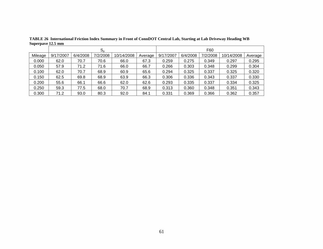
61
TABLE 26 International Friction Index Summary in Front of ConnDOT Central Lab, Starting at Lab Driveway Heading WB
Superpave 12.5 mm
Sp F60
Mileage 9/17/2007 6/4/2008 7/2/2008 10/14/2008 Average 9/17/2007 6/4/2008 7/2/2008 10/14/2008 Average
0.000 62.0 70.7 70.6 66.0 67.3 0.259 0.275 0.349 0.297 0.295
0.050 57.9 71.2 71.6 66.0 66.7 0.266 0.303 0.348 0.299 0.304
0.100 62.0 70.7 68.9 60.9 65.6 0.294 0.325 0.337 0.325 0.320
0.150 62.5 69.8 68.9 63.9 66.3 0.306 0.336 0.343 0.337 0.330
0.200 55.6 66.1 66.6 62.0 62.6 0.293 0.335 0.337 0.334 0.325
0.250 59.3 77.5 68.0 70.7 68.9 0.313 0.360 0.348 0.351 0.343
0.300 71.2 93.0 80.3 92.0 84.1 0.331 0.369 0.366 0.362 0.357
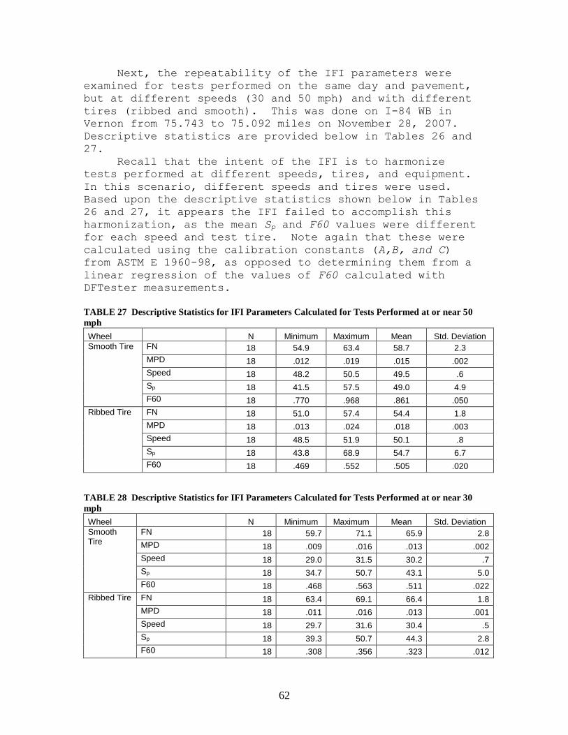
62
Next, the repeatability of the IFI parameters were
examined for tests performed on the same day and pavement,
but at different speeds (30 and 50 mph) and with different
tires (ribbed and smooth). This was done on I-84 WB in
Vernon from 75.743 to 75.092 miles on November 28, 2007.
Descriptive statistics are provided below in Tables 26 and
27.
Recall that the intent of the IFI is to harmonize
tests performed at different speeds, tires, and equipment.
In this scenario, different speeds and tires were used.
Based upon the descriptive statistics shown below in Tables
26 and 27, it appears the IFI failed to accomplish this
harmonization, as the mean Sp and F60 values were different
for each speed and test tire. Note again that these were
calculated using the calibration constants (A,B, and C)
from ASTM E 1960-98, as opposed to determining them from a
linear regression of the values of F60 calculated with
DFTester measurements.
TABLE 27 Descriptive Statistics for IFI Parameters Calculated for Tests Performed at or near 50
mph
Wheel N Minimum Maximum Mean Std. Deviation
Smooth Tire
FN 18 54.9 63.4 58.7 2.3
MPD 18 .012 .019 .015 .002
Speed 18 48.2 50.5 49.5 .6
Sp 18 41.5 57.5 49.0 4.9
F60 18 .770 .968 .861 .050
Ribbed Tire
FN 18 51.0 57.4 54.4 1.8
MPD 18 .013 .024 .018 .003
Speed 18 48.5 51.9 50.1 .8
Sp 18 43.8 68.9 54.7 6.7
F60 18 .469 .552 .505 .020
TABLE 28 Descriptive Statistics for IFI Parameters Calculated for Tests Performed at or near 30
mph
Wheel N Minimum Maximum Mean Std. Deviation
Smooth Tire
FN 18 59.7 71.1 65.9 2.8
MPD 18 .009 .016 .013 .002
Speed 18 29.0 31.5 30.2 .7
Sp 18 34.7 50.7 43.1 5.0
F60 18 .468 .563 .511 .022
Ribbed Tire
FN 18 63.4 69.1 66.4 1.8
MPD 18 .011 .016 .013 .001
Speed 18 29.7 31.6 30.4 .5
Sp 18 39.3 50.7 44.3 2.8
F60 18 .308 .356 .323 .012
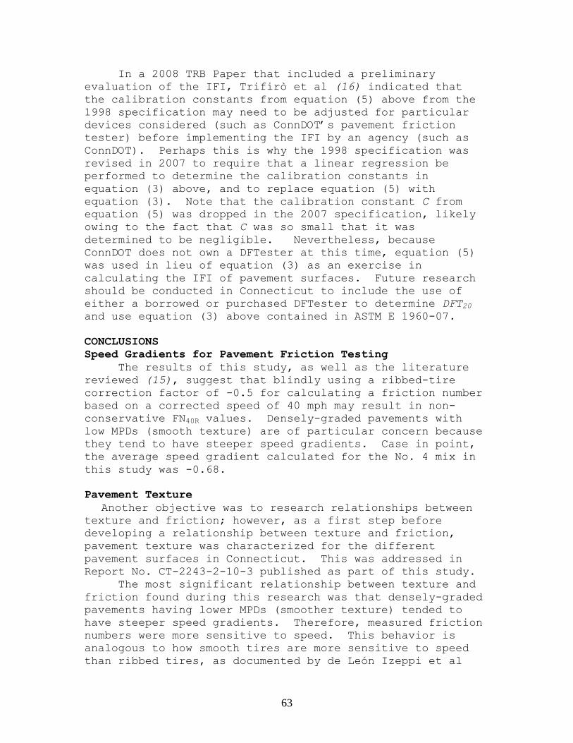
63
In a 2008 TRB Paper that included a preliminary
evaluation of the IFI, Trifirò et al (16) indicated that
the calibration constants from equation (5) above from the
1998 specification may need to be adjusted for particular
devices considered (such as ConnDOT’s pavement friction
tester) before implementing the IFI by an agency (such as
ConnDOT). Perhaps this is why the 1998 specification was
revised in 2007 to require that a linear regression be
performed to determine the calibration constants in
equation (3) above, and to replace equation (5) with
equation (3). Note that the calibration constant C from
equation (5) was dropped in the 2007 specification, likely
owing to the fact that C was so small that it was
determined to be negligible. Nevertheless, because
ConnDOT does not own a DFTester at this time, equation (5)
was used in lieu of equation (3) as an exercise in
calculating the IFI of pavement surfaces. Future research
should be conducted in Connecticut to include the use of
either a borrowed or purchased DFTester to determine DFT20
and use equation (3) above contained in ASTM E 1960-07.
CONCLUSIONS
Speed Gradients for Pavement Friction Testing
The results of this study, as well as the literature
reviewed (15), suggest that blindly using a ribbed-tire
correction factor of -0.5 for calculating a friction number
based on a corrected speed of 40 mph may result in non-
conservative FN40R values. Densely-graded pavements with
low MPDs (smooth texture) are of particular concern because
they tend to have steeper speed gradients. Case in point,
the average speed gradient calculated for the No. 4 mix in
this study was -0.68.
Pavement Texture
Another objective was to research relationships between
texture and friction; however, as a first step before
developing a relationship between texture and friction,
pavement texture was characterized for the different
pavement surfaces in Connecticut. This was addressed in
Report No. CT-2243-2-10-3 published as part of this study.
The most significant relationship between texture and
friction found during this research was that densely-graded
pavements having lower MPDs (smoother texture) tended to
have steeper speed gradients. Therefore, measured friction
numbers were more sensitive to speed. This behavior is
analogous to how smooth tires are more sensitive to speed
than ribbed tires, as documented by de León Izeppi et al
64
(15). This likely owes to water having an escape route for
more open-textured (higher MPDs) pavements at higher
speeds, whereas water does not have an escape route for
densely-textured (lower MPDs) pavements. Higher speeds
tend to compound this phenomenon.
The entire report will not be duplicated here, but the
conclusions from CT-2243-2-10-3 are listed below once again
in this, the final report published for this research.
Scatter plots showing the relationship between mean
profile depth (MPD) values measured with the high-speed
laser instrument mounted to the friction tester versus
values measured with the CTMeter were analyzed. The
linear association between these variables was relatively
strong, as coefficients of determination (R2
coefficients) of 0.65 and 0.87 were calculated for the VA
Smart Road and CT SPS 9A sites, respectively. As such,
the high-speed laser instrument appears to provide viable
relative macrotexture measurements.
In response to a FHWA Technical Advisory titled Surface
Texture for Asphalt and Concrete Pavements, ConnDOT has
begun to establish targets for pavement texture depth on
high-speed facilities by characterizing the macrotexture
of a few different ConnDOT HMA pavement mixes. The mean
profile depth or MPD appears to be the best measure for
characterizing pavement macrotexture, since it can be
measured using either the high-speed laser instrument or
CTMeter.
The characterizing MPDs measured for ConnDOT mixes ranged
between .021 and .022 inches (0.53 to 0.56 mm) for the
12.5-mm Superpave design, .015 inches (0.38 mm) for 9.5-
mm Superpave design, .012 to .015 inches (0.30 to 0.38
mm) for the 6.35-mm Superpave design, and 0 to .004
inches (0 to 10 mm) for the 4.75-mm design. These
characterizing values are still preliminary and more
research is needed to determine the best application(s)
for each pavement design.
There was a linear association between measured MPD
values and the percents passing the #4 and #8 sieves for
a respective pavement’s grain-size distribution. MPD
values tended to increase as mixes became coarser.
Laser profiler macrotexture measurements were repeatable
from one day to the next. 399 macrotexture measurements
were taken on the same 9.5-mm Superpave mix on I-91 NB in
Connecticut, and the mean MPD for these measurements was
.015 inches (0.38 mm) on both days. The standard
65
deviation was also identical on both days (+/- .0027
inches or 0.069 mm).
The ConnDOT CTMeter compared almost identically to the
Virginia Tech CTMeter at the Smart Road facility in
Blacksburg, VA during an equipment Rodeo.
International Friction Index (IFI)
The intent of the IFI is to harmonize tests performed
at different speeds, tires, and equipment. As part of this
research, IFI parameters were calculated using the
calibration constants (A,B, and C) from tables contained in
ASTM E 1960-98. The results of his research suggest that
the IFI calculated using the above calibration constants
was not effective in harmonizing tests performed at
different speeds and tires. The latest ASTM E 1960 (2007)
specification requires that these constants be determined
from a linear regression of the values of F60 calculated
with DFTester measurements, as opposed to using values from
tables. Note: ConnDOT does not currently own a DFTester.
Effect of Roadway Geometry on Friction Measurements
A short study of the effects of horizontal and
vertical alignment on friction measurements was performed.
The testing along horizontal curves was performed at the
Consumer Union Test Track in Colchester, CT. The testing
along vertical curves was performed on Route 66 in
Marlborough, CT.
Friction tests were performed along horizontal curves
of 24 and 28 degrees, and were compared to tests performed
along straight tangents of the same pavement. The average
FN40R values increased slightly for sharper degrees of
curvature, but valid statistical conclusions can not be
drawn without more data. In general, the ranges within
which tangent and nontangent FN40R values occurred were
similar.
In order to obtain more data, more testing of this
nature would need to be performed. The testing that was
performed was carried out at the Consumer Union Test Track.
Unfortunately, ConnDOT does not own a track, so special
arrangements would be required for additional testing.
Therefore, it is concluded that continued research of this
nature would be better suited for organizations that own or
have regular access to a test track.
This research was successful at demonstrated that
comparable results are obtainable, even when the friction
tester is pushed to its limits along sharp horizontal
curves. Note that these tests were performed along these
66
curves without any superelevation. The banking
capabilities provided by superelevated pavement would
further enhance the friction tester’s ability to perform
valid tests.
Literature related to tangent versus nontangent
sections was reviewed (14). Zimmer and Tonda indicated
that friction test results were similar between tangent and
nontangent sections, but they suggested limiting the
horizontal g-force on the skid trailer to 0.3 g’s. They
also suggested performing tests along horizontal curves
during dry pavement conditions, because virtually all of
the traction forces are transferred to the non-test wheel
during testing. Dry conditions along the non-test wheel
will therefore provide greater side-force traction to
maintain the skid trailer on the roadway without sliding.
The testing that was performed on positive versus
negative grades also demonstrated that similar results
between these vertical grades are obtainable.
RECOMMENDATIONS
Speed Gradients for Pavement Friction Testing
It is recommended that for instances where friction
testing cannot be performed at 40 mph, FN40R and FN40S be
calculated using the following formulas:
FN40R = FN + (speed gradient)*(40-speed)
or
FN40S = FN + (speed gradient)*(40-speed)
These speed gradients should be determined on a case-
by-case basis in accordance with ASTM E 274 Section 7.6.
For sharp horizontal curves, the speed gradient of adjacent
pavement of the same mix and construction should be tested
to determine the gradient.
For situations where individual speed gradients cannot
be determined, it is recommended that a FN40R envelope be
determined using speed gradient values between -0.3 and -
0.7. This would provide more conservative FN40R values, and
avoid the use of non-conservative values. Special
attention should be given to dense-graded pavement
surfaces, as these pavements are more sensitive to test
speed.
67
Pavement Texture
The following recommendations from Report No CT-2243-
2-10-3 are presented below (3):
Mean profile depths (MPDs) measured with the high-speed
laser instrument are adequate for providing relative
values for characterizing pavement macrotexture on
typical HMA pavements used in Connecticut. These typical
pavements include but are not limited to 12.5-mm, 9.5-mm,
6.35-mm, and 4.75-mm HMA mixes. Care should be taken in
exercising these measurements for other pavements. To
that end, it is recommended that further comparative
testing be performed between the high-speed laser
instrument and other proven instruments, such as the
CTMeter, prior to exercising high-speed laser
measurements for uncommon pavements. Uncommon pavements
in Connecticut include but are not limited to portland
cement concrete (PCC) pavements, open-graded friction
courses, and other surface treatments.
Until demonstrated otherwise, the #4 mix (4.75-mm) should
not be used to pave high-speed (50-mph or greater)
facilities because it does not appear to have adequate
texture depth in comparison to the other mixes evaluated.
This mix should be used only on low-speed facilities that
require very thin pavement lifts, but an evaluation of
the site geometrics, traffic levels, and vehicle speeds
should be conducted before selecting this mix.
Until demonstrated otherwise, ConnDOT should continue to
use the 12.5-mm Superpave mix for high-speed facilities
because it appears to provide the most texture depth of
the pavements evaluated.
The 6.35-mm and 9.5-mm Superpave mixes had grain-size
distributions that were similar to one another, and each
provided approximately the same level of surface texture.
These mixes appear to provide marginal levels of surface
texture for high-speed roadways in comparison to the
12.5-mm Superpave mix evaluated in this study. These
mixes should provide an adequate level of surface texture
for low-speed roadways, although an evaluation of the
site geometrics, traffic levels, and vehicle speeds
should be conducted before selecting these mixes.
Continued use for high-speed roadways for special
applications should be monitored by performing periodic
friction (smooth and ribbed tire) and texture
measurements.
68
International Friction Index (IFI)
At this time, the IFI is not recommended for
implementation. Further research should be conducted to
evaluate the IFI in conjunction with the latest update to
ASTM E 1960-07 which includes DFTester measurements for
calibration constant determinations. Accordingly, a
DFTester should be purchased.
Roadway Geometry
An accelerometer should be purchased and mounted to
the skid trailer to measure the horizontal g-forces that
occur during testing along nontangent sections.
Smooth- and Ribbed-Tires for Friction Testing
Based upon the literature reviewed, it is recommended
that both the ASTM E501 Standard Rib Tire and ASTM E524
Standard Smooth Tire be used for pavement friction testing
performed in response to requests received for safety
evaluation purposes. Tentative guidelines for evaluating
friction at high wet accident sites are provided in
Appendix A.
DELIVERABLES
Deliverables for this project include the following
products:
Upgraded pavement friction tester
CTMeter
Quarterly progress reports
ConnDOT Report No. CT-2243-1-10-1 titled “Historical
Overview of Friction Testing in Connecticut”
ConnDOT Report No. CT-2243-2-10-3 titled “Characterizing
the Macrotexture of Asphalt Pavement Designs in
Connecticut”
This Final Report No. CT-2243-F-10-4
Meet the Author Poster Session presented at the 89th TRB
Annual Meeting in Washington, D.C. in Session Number 580,
“Traveled Surface Texture, Friction, Noise, and Profile.”
A trading card for the overall project, and for CT-2243-
1-10-1, which was presented in Washington, D.C. in a
poster session.
ConnDOT Video on Demand: About ConnDOT’s Pavement
Friction Testing and Safety Evaluation Program,
http://www.ct.gov/dot/cwp/view.asp?a=1617&q=273484#b10,
presented on March 27, 2008.
ConnDOT Video on Demand: Pavement Surface Properties
Consortium: A Collaborative Research Program,
69
http://www.ct.gov/dot/cwp/view.asp?a=1617&q=448232,
recorded on September 24, 2009.
IMPLEMENTATION
Another objective of this research was to implement
the appropriate latest technology and procedures for
pavement friction data request, collection, and processing.
As part of the effort to implement the latest
technology for pavement friction data requests, a draft web
page was developed by a Summer Worker during the summer of
2008. The web page included links to “fillable” pdf’s and
to historical friction testing memorandum. The “fillable”
pdf’s would be used by any ConnDOT unit to request pavement
friction tests.
The Summer Worker has since moved on, but the web page
draft still exists and is available. A copy of the web
page is presented in Appendix B.
In this report, recommendations were made regarding
speed gradients and their application, use of smooth and
ribbed tires, pavement texture, and literature was reviewed
regarding intervention levels. In the context of
implementing findings, draft friction testing procedures
and a draft policy statement are presented in Appendices C
and D, respectively, which address the above
recommendations.
REFERENCES
1. Larsen, D.A., and E.G. Feldblum. Enhancements to ConnDOT’s Pavement Friction Testing Program. Proposal No.
P-04-1. Connecticut Department of Transportation, 2004.
2. Henault, J.W. Historical Overview of Pavement Friction Testing in Connecticut. Report No. CT-2243-1-10-1.
Connecticut Department of Transportation, 2010.
3. Henault, J.W., and J. Bliven. Characterizing the Macrotexture of Asphalt Pavement Designs in Connecticut.
Report No. CT-2243-2-10-3. Connecticut Department of
Transportation, February 2011.
4. Dynatest 1295 Pavement Friction Tester Operation Manual, Version 1.01, Dynatest, Westland, MI, April 2003.
5. Transportation Pooled Fund Program, TPF-5(141), Pavement surface Propeties Consortium: A Research Program, NCHRP,
http://www.pooledfund.org/projectdetails.asp?id=371&statu
s=4, Accessed December 3, 2008.
6. U.S. Department of Transportation Federal Highway Administration, Surface Texture for Asphalt and Concrete
Pavements, Technical Advisory, Classification Code T
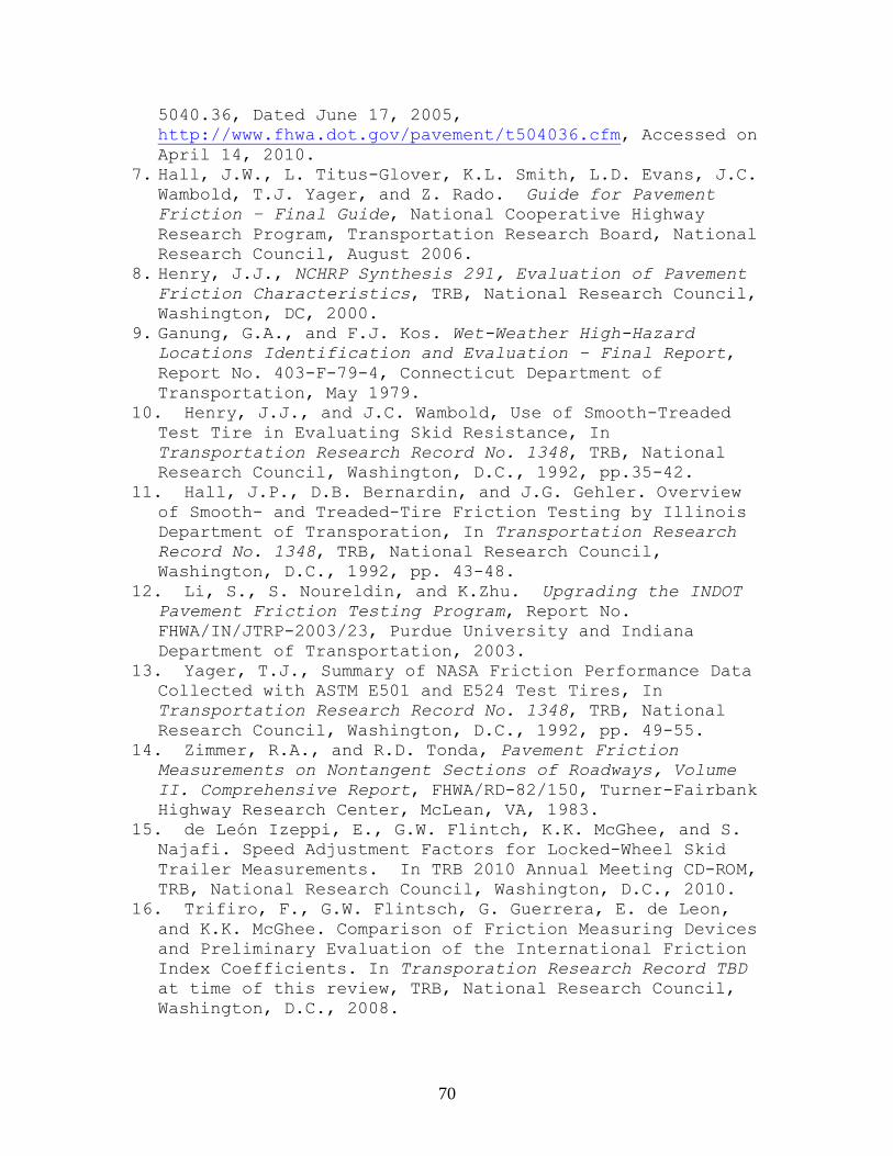
70
5040.36, Dated June 17, 2005,
http://www.fhwa.dot.gov/pavement/t504036.cfm, Accessed on
April 14, 2010.
7. Hall, J.W., L. Titus-Glover, K.L. Smith, L.D. Evans, J.C. Wambold, T.J. Yager, and Z. Rado. Guide for Pavement
Friction – Final Guide, National Cooperative Highway
Research Program, Transportation Research Board, National
Research Council, August 2006.
8. Henry, J.J., NCHRP Synthesis 291, Evaluation of Pavement Friction Characteristics, TRB, National Research Council,
Washington, DC, 2000.
9. Ganung, G.A., and F.J. Kos. Wet-Weather High-Hazard Locations Identification and Evaluation – Final Report,
Report No. 403-F-79-4, Connecticut Department of
Transportation, May 1979.
10. Henry, J.J., and J.C. Wambold, Use of Smooth-Treaded
Test Tire in Evaluating Skid Resistance, In
Transportation Research Record No. 1348, TRB, National
Research Council, Washington, D.C., 1992, pp.35-42.
11. Hall, J.P., D.B. Bernardin, and J.G. Gehler. Overview
of Smooth- and Treaded-Tire Friction Testing by Illinois
Department of Transporation, In Transportation Research
Record No. 1348, TRB, National Research Council,
Washington, D.C., 1992, pp. 43-48.
12. Li, S., S. Noureldin, and K.Zhu. Upgrading the INDOT
Pavement Friction Testing Program, Report No.
FHWA/IN/JTRP-2003/23, Purdue University and Indiana
Department of Transportation, 2003.
13. Yager, T.J., Summary of NASA Friction Performance Data
Collected with ASTM E501 and E524 Test Tires, In
Transportation Research Record No. 1348, TRB, National
Research Council, Washington, D.C., 1992, pp. 49-55.
14. Zimmer, R.A., and R.D. Tonda, Pavement Friction
Measurements on Nontangent Sections of Roadways, Volume
II. Comprehensive Report, FHWA/RD-82/150, Turner-Fairbank
Highway Research Center, McLean, VA, 1983.
15. de León Izeppi, E., G.W. Flintch, K.K. McGhee, and S.
Najafi. Speed Adjustment Factors for Locked-Wheel Skid
Trailer Measurements. In TRB 2010 Annual Meeting CD-ROM,
TRB, National Research Council, Washington, D.C., 2010.
16. Trifiro, F., G.W. Flintsch, G. Guerrera, E. de Leon,
and K.K. McGhee. Comparison of Friction Measuring Devices
and Preliminary Evaluation of the International Friction
Index Coefficients. In Transporation Research Record TBD
at time of this review, TRB, National Research Council,
Washington, D.C., 2008.

71
17. Kummer, H.W., and Meyer, W.E., Tentative Skid-
Resistance Requirements for Main Rural Highways, NCHRP
Report 37, National Cooperative Highway Research Program,
1967.
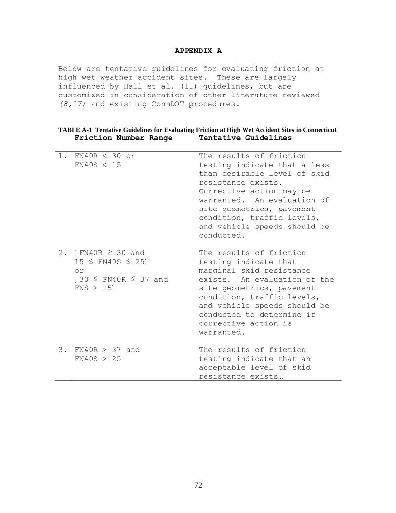
72
APPENDIX A
Below are tentative guidelines for evaluating friction at
high wet weather accident sites. These are largely
influenced by Hall et al. (11) guidelines, but are
customized in consideration of other literature reviewed
(8,17) and existing ConnDOT procedures.
TABLE A-1 Tentative Guidelines for Evaluating Friction at High Wet Accident Sites in Connecticut
Friction Number Range Tentative Guidelines
1. FN40R < 30 or
FN40S < 15
The results of friction
testing indicate that a less
than desirable level of skid
resistance exists.
Corrective action may be
warranted. An evaluation of
site geometrics, pavement
condition, traffic levels,
and vehicle speeds should be
conducted.
2. [FN40R ≥ 30 and
15 ≤ FN40S ≤ 25]
or
[30 ≤ FN40R ≤ 37 and
FNS > 15]
The results of friction
testing indicate that
marginal skid resistance
exists. An evaluation of the
site geometrics, pavement
condition, traffic levels,
and vehicle speeds should be
conducted to determine if
corrective action is
warranted.
3. FN40R > 37 and
FN40S > 25
The results of friction
testing indicate that an
acceptable level of skid
resistance exists…
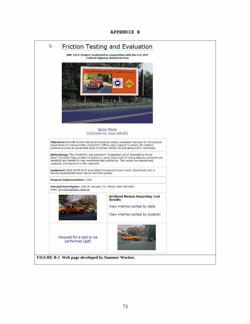
73
APPENDIX B
FIGURE B-1 Web page developed by Summer Worker.
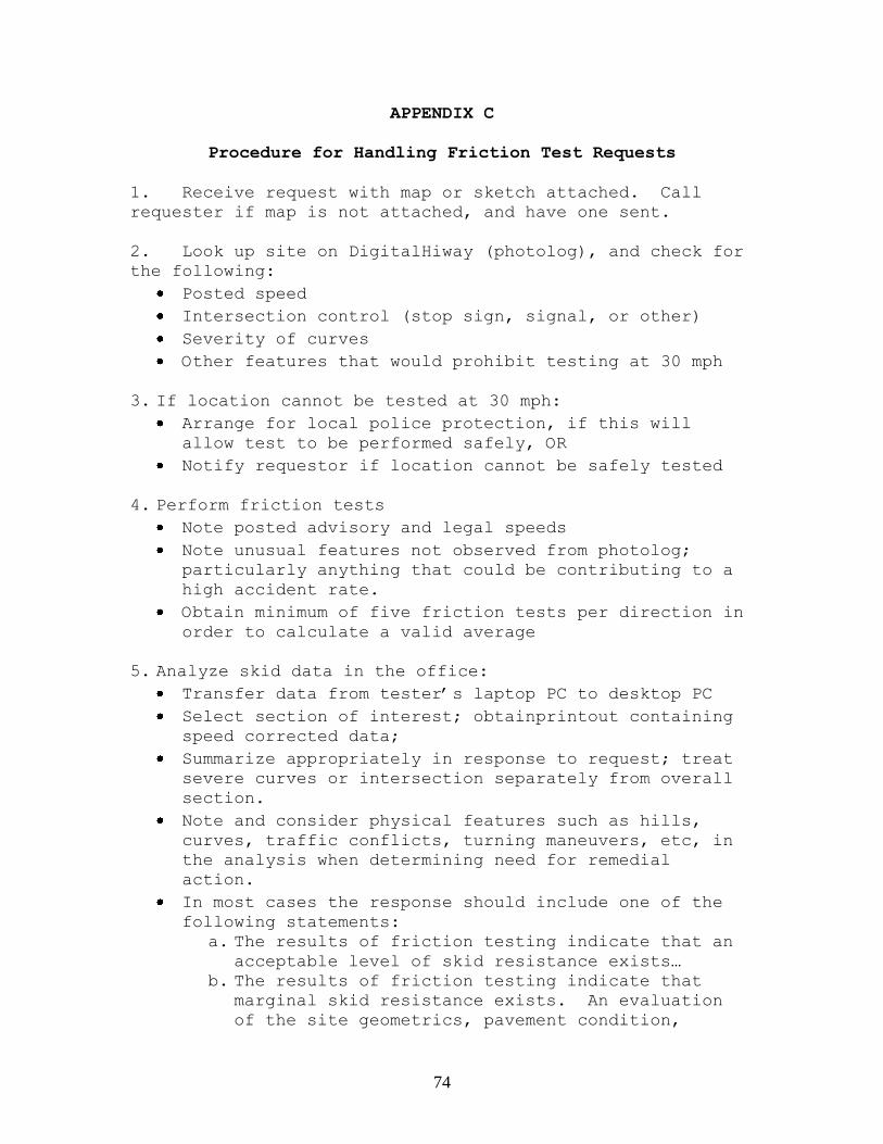
74
APPENDIX C
Procedure for Handling Friction Test Requests
1. Receive request with map or sketch attached. Call
requester if map is not attached, and have one sent.
2. Look up site on DigitalHiway (photolog), and check for
the following:
Posted speed
Intersection control (stop sign, signal, or other)
Severity of curves
Other features that would prohibit testing at 30 mph
3. If location cannot be tested at 30 mph:
Arrange for local police protection, if this will
allow test to be performed safely, OR
Notify requestor if location cannot be safely tested
4. Perform friction tests
Note posted advisory and legal speeds
Note unusual features not observed from photolog;
particularly anything that could be contributing to a
high accident rate.
Obtain minimum of five friction tests per direction in
order to calculate a valid average
5. Analyze skid data in the office:
Transfer data from tester’s laptop PC to desktop PC
Select section of interest; obtainprintout containing
speed corrected data;
Summarize appropriately in response to request; treat
severe curves or intersection separately from overall
section.
Note and consider physical features such as hills,
curves, traffic conflicts, turning maneuvers, etc, in
the analysis when determining need for remedial
action.
In most cases the response should include one of the
following statements:
a. The results of friction testing indicate that an acceptable level of skid resistance exists…
b. The results of friction testing indicate that marginal skid resistance exists. An evaluation
of the site geometrics, pavement condition,
75
traffic levels, and vehicle speeds should be
conducted to determine if corrective action is
warranted.
c. The results of friction testing indicate that a less than desirable level of skid resistance
exists. Corrective action may be warranted. An
evaluation of site geometrics, pavement
condition, traffic levels, and vehicle speeds
should be conducted.
6. Prepare memo and send results to requesting party. Copies of the memo shall be forwarded to Transportation
Maintenance, Maintenance Operations, Maintenance
Planning, Traffic Engineering, and Pavement Management.
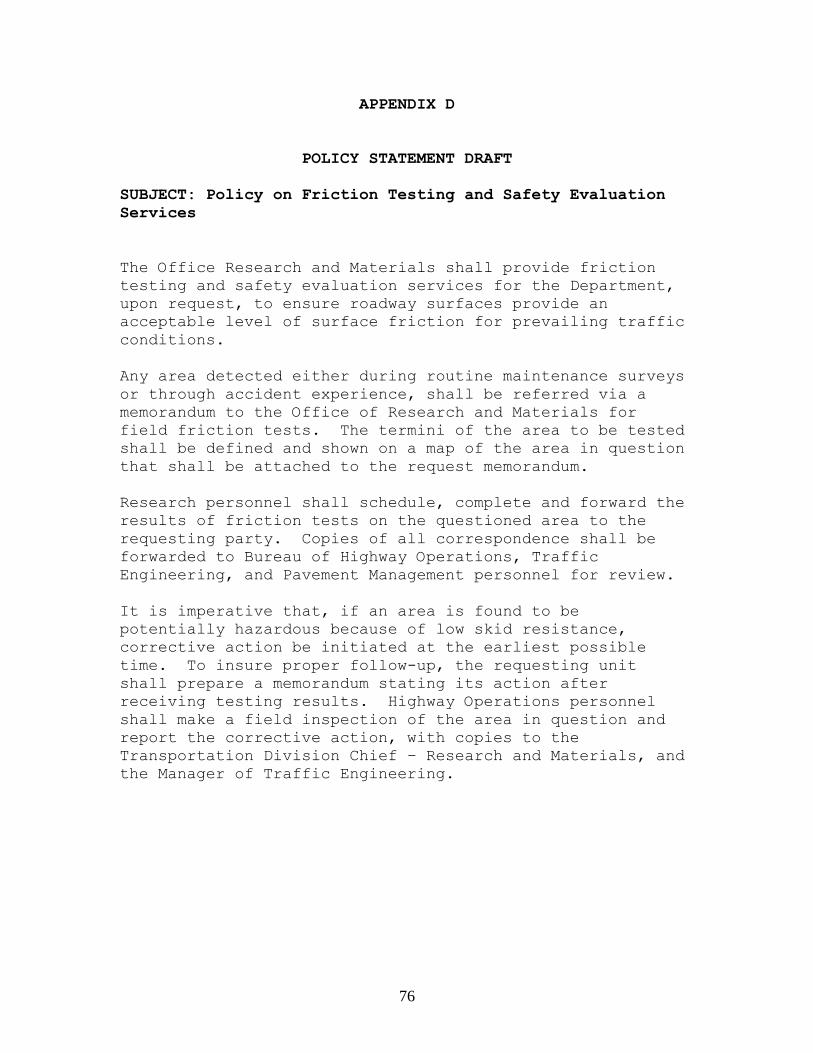
76
APPENDIX D
POLICY STATEMENT DRAFT
SUBJECT: Policy on Friction Testing and Safety Evaluation
Services
The Office Research and Materials shall provide friction
testing and safety evaluation services for the Department,
upon request, to ensure roadway surfaces provide an
acceptable level of surface friction for prevailing traffic
conditions.
Any area detected either during routine maintenance surveys
or through accident experience, shall be referred via a
memorandum to the Office of Research and Materials for
field friction tests. The termini of the area to be tested
shall be defined and shown on a map of the area in question
that shall be attached to the request memorandum.
Research personnel shall schedule, complete and forward the
results of friction tests on the questioned area to the
requesting party. Copies of all correspondence shall be
forwarded to Bureau of Highway Operations, Traffic
Engineering, and Pavement Management personnel for review.
It is imperative that, if an area is found to be
potentially hazardous because of low skid resistance,
corrective action be initiated at the earliest possible
time. To insure proper follow-up, the requesting unit
shall prepare a memorandum stating its action after
receiving testing results. Highway Operations personnel
shall make a field inspection of the area in question and
report the corrective action, with copies to the
Transportation Division Chief – Research and Materials, and
the Manager of Traffic Engineering.