Embed Size (px)
Citation preview
University of Central Florida University of Central Florida
STARS STARS
Electronic Theses and Dissertations, 2004-2019
2015
Enhanced Microwave Hyperthermia using Nanoparticles Enhanced Microwave Hyperthermia using Nanoparticles
Maryory Urdaneta University of Central Florida
Part of the Electrical and Electronics Commons
Find similar works at: https://stars.library.ucf.edu/etd
University of Central Florida Libraries http://library.ucf.edu
This Doctoral Dissertation (Open Access) is brought to you for free and open access by STARS. It has been accepted
for inclusion in Electronic Theses and Dissertations, 2004-2019 by an authorized administrator of STARS. For more
information, please contact [email protected].
STARS Citation STARS Citation Urdaneta, Maryory, "Enhanced Microwave Hyperthermia using Nanoparticles" (2015). Electronic Theses and Dissertations, 2004-2019. 1189. https://stars.library.ucf.edu/etd/1189
ENHANCED MICROWAVE HYPERTHERMIA USING NANOPARTICLES
by
MARYORY URDANETA M.S. University of Central Florida, 2012
A dissertation submitted in partial fulfillment of the requirements
for the degree of Doctor of Philosophy
in the Department of Electrical Engineering and Computer Science
in the College of Engineering and Computer Science
at the University of Central Florida
Orlando, Florida
Spring Term
2015
Major Professor: Parveen Wahid
ii
ABSTRACT
In this dissertation a study of enhanced hyperthermia for cancer treatment through the use of
magnetic nanoparticles is presented. Hyperthermia has been in use for many years, as a potential
alternative method in cancer treatment, and high frequency microwave radiation has been used
successfully to raise the tumor temperature to around 42C in superficial tumors without causing
damage to surrounding healthy tissues. Magnetic fluid hyperthermia involves the use of
magnetic nanoparticles injected into the tumor before exposure to microwave radiation. The
magnetic energy in the nanoparticles is converted into heat allowing for a more rapid rise of
temperature in the tumor to the desired level. In addition, the nanoparticles allow the
electromagnetic absorption to be focused in the tumor and can be used to treat deep tumors in
organs, such as the liver. Iron oxide magnetic nanoparticles were considered for this study as
they are non-toxic and bio-compatible. For the case of breast cancer, the values for the
temperature and specific absorption rate (SAR) in the tumor and in the healthy tissue were
obtained through simulations and validated by measurement done on phantom models. Various
characteristics of the nanoparticles such as radius, magnetic susceptibility and concentration
were considered. In order to take the effect of the blood flow, which causes cooling and helps
maintain the body temperature, various blood perfusion rates for a tumor in the liver were
studied. A human male model in SEMCAD X, in which blood flow can be adjusted, was used for
simulations. The tumor was injected with the nanoparticles and the change in temperature upon
exposure to electromagnetic radiation was observed. The simulated results were compared with
measured results on a liver phantom model in which saline solution was used to model blood
flow. There was good agreement between the measured and simulated results.
iii
ACKNOWLEDGMENTS
I would like to thank my advisor Dr. Wahid for all her support, guidance and patient
during my studies at UCF. Thanks for giving me the opportunity to work with you. I could not
ask for more from you. I also appreciate the helpful teachings and guidance of my dissertation
committee members: Prof. Xun Gong, Prof. Kalpathy Sundaram, Prof. Samuel Richie and Prof.
Suryanarayana Challapalli.
I also thankfully acknowledge SEMCAD X for providing the simulation tools to
accomplish this research.
I am thankful to the Fulbright Scholarship program for their support at the beginning of
my career. Without their support I would not have started this amazing adventure.
Thanks to all of my course professors. I learned so much from all of you that will surely
benefit me for the rest of my life.
I am eternally grateful to my family who has supported me throughout my life, even from
a distance. I thank my mother Marisela for her enduring love, support and patience. I would not
have completed this step in my career without you in my corner.
I am truly thankful to all members of the ARMI lab at UCF who generously offered their
time to help anytime I needed it.
Thanks to my alma mater Universidad del Zulia for their support me throughout all these
years.
iv
TABLE OF CONTENTS
LIST OF FIGURES ....................................................................................................................... vi
LIST OF TABLES ....................................................................................................................... viii
CHAPTER 1: INTRODUCTION ................................................................................................... 1
1.1. Overview of Medical Applications of High Frequency Radiation ....................................... 1
1.1.1. Microwave Imaging ....................................................................................................... 1
1.1.2. Thermal Therapy ........................................................................................................... 2
1.2. Motivation for the Research ................................................................................................. 4
1.3. Dissertation Outline.............................................................................................................. 5
CHAPTER 2: BIOLOGICAL AND PHYSICAL ASPECTS OF HYPERTHERMIA .................. 7
2.1. RF/Microwave Propagation in Biological Tissues............................................................... 7
2.2. Electromagnetic Waves Propagating in Biological Tissues ................................................. 7
2.3. Hyperthermia ...................................................................................................................... 11
2.4. Hyperthermia Applicators .................................................................................................. 12
2.4.1. Inductive Heating ........................................................................................................ 13
2.4.2. Capacitive Heating ...................................................................................................... 13
2.4.3. Radiation Heating ........................................................................................................ 14
2.4.4. Interstitial Applicators ................................................................................................. 14
CHAPTER 3: HEAT TRANSFER IN HYPERTHERMIA.......................................................... 15
3.1. Introduction ........................................................................................................................ 15
3.2. Penne’s Bioheat Equation .................................................................................................. 15
3.3. Specific Absorption Rate (SAR) ........................................................................................ 16
CHAPTER 4: MAGNETIC FLUID HYPERTHERMIA ............................................................. 19
4.1. Introduction ........................................................................................................................ 19
4.2. Nanoparticle Targeting ....................................................................................................... 20
4.3. Heat Generation of Nanoparticles ...................................................................................... 20
4.3.1. Hysteresis..................................................................................................................... 21
4.3.2. Relaxation .................................................................................................................... 22
CHAPTER 5: MICROWAVE MAGNETIC FLUID HYPERTHERMIA MODELING ........... 29
v
5.1. Introduction ........................................................................................................................ 29
5.2. Magnetic Fluid Hyperthermia Design Considerations ....................................................... 29
5.3. Heat Generation.................................................................................................................. 30
5.4. Simulation .......................................................................................................................... 31
5.5. Temperature Measurements using SEMCAD X ................................................................ 32
5.6. Effect of Nanoparticle Characteristics in the Transient Temperature in the Tumor .......... 35
5.6.1. Nanoparticle Size ......................................................................................................... 36
5.6.2. Nanoparticle Susceptibility .......................................................................................... 38
5.6.3. Effect of Nanoparticle Concentration on the Heating Behavior .................................. 38
5.6.4. Optimization of Nanoparticle Concentration .............................................................. 39
5.7. Experimental Results.......................................................................................................... 41
5.7.1. Solid Phantom.............................................................................................................. 41
5.7.2. Measurement Setup ..................................................................................................... 43
5.7.3. Temperature Measurements ........................................................................................ 43
CHAPTER 6: MAGNETIC FLUID HYPERTHERMIA INCORPORATING BLOOD FLOW 46
6.1. Introduction ........................................................................................................................ 46
6.2. Blood Perfusion in Humans ............................................................................................... 46
6.3. Magnetic Fluid Hyperthermia Design Incorporating the Blood Perfusion ........................ 48
6.4. Simulated Transient Temperature ...................................................................................... 50
6.5. Experimental Results using a Simplified Phantom ............................................................ 56
6.6. Measured Temperatures ..................................................................................................... 59
6.7. Use of Magnetic Fluid Hyperthermia in Human Tissues ................................................... 62
CHAPTER 7: CONCLUSIONS ................................................................................................... 63
REFERENCES ............................................................................................................................. 65
vi
LIST OF FIGURES
Figure 1. Microwave imaging of breast tissue ................................................................................ 2
Figure 2. Electric field propagation in biological tissues ............................................................... 8
Figure 3. Relative absorbed power in fat and muscle as a distance function at 2.45 GHz ............. 9
Figure 4. a) Large particles hysteresis, b) Small particles hysteresis and c) Smaller particles
hysteresis ....................................................................................................................................... 21
Figure 5. Real and imaginary components of the susceptibility vs. Frequency ........................... 25
Figure 6. Hyperthermia system configuration .............................................................................. 29
Figure 7. Breast tissue model in SEMCAD X .............................................................................. 32
Figure 8. Tempertaure distribution during hyperthermia without nanoparticles .......................... 33
Figure 9. Tempertaure distribution during hyperthermia with nanoparticles ............................... 34
Figure 10. Time temperature increase in the tissue as function of distance from the applicator .. 35
Figure 11. Transient temperature in the tumor for different nanoparticles sizes .......................... 36
Figure 12. Néel relaxation time 𝜏𝑁 as a function of radius of the nanoparticle ........................... 37
Figure 13. Transient temperature in the tumor for different nanoparticles susceptibilities .......... 38
Figure 14. Transient temperature in the tumor with different nanoparticles concentrations ........ 39
Figure 15. Solid phantom simulating the human breast tissue ..................................................... 42
Figure 16. Ferrofluid conatining the nanoparticles and tumor phantom ...................................... 42
Figure 17. Measurement setup ...................................................................................................... 43
Figure 18. Temperature in phantom without nanoparticles .......................................................... 44
Figure 19. Temperature in phantom with nanoparticles ............................................................... 45
Figure 20. Human model in SEMCAD X ..................................................................................... 49
Figure 21. Transient temperature in the l.iver model – Blood perfusion rate 100% .................... 51
Figure 22. Transient temperature in the l.iver model – Blood perfusion rate 75% ...................... 51
Figure 23. Transient temperature in the liver model – Blood perfusion rate 50% ....................... 52
Figure 24. Transient temperature in the l.iver model – Blood perfusion rate 25% ...................... 52
Figure 25. Transient temperature in the l.iver model – Blood perfusion rate 5% ........................ 53
Figure 26. Temperature comparison in the tumor and healthy tissue ........................................... 54

vii
Figure 27. SAR comparison in the tumor and healthy tissue ....................................................... 54
Figure 28. Temperature increase in the tumor as a function of nanoparticle concentration ......... 55
Figure 29. Simplified liver model ................................................................................................. 56
Figure 30. Liver phantom measurement setup – Side view .......................................................... 58
Figure 31. Liver phantom model – Top view ............................................................................... 58
Figure 32. Temperature measured in healthy and tumor tissues in the model 1 .......................... 59
Figure 33. Temperature measured in healthy and tumor tissues in the model 2 .......................... 60
Figure 34. Temperature measured in healthy and tumor tissues in the model 3 .......................... 60
Figure 35. Temperature measured in healthy and tumor tissues in the model 4 .......................... 61
Figure 36. Temperature measured in healthy and tumor tissues in the model 5 .......................... 61
viii
LIST OF TABLES
Table 1. Dielectric properties of human tissues at different frequencies ...................................... 10
Table 2. Basic restrictions for time varying electric and magnetic fields for frequencies up to 10
GHz. .............................................................................................................................................. 17
Table 3. Electrical properties of human tissues ............................................................................ 30
Table 4. Thermal properties of human and tumor tissues ............................................................. 31
Table 5. Blood perfusion in human tissues ................................................................................... 47
Table 6. Models with different blood perfusion rates ................................................................... 50
1
CHAPTER 1: INTRODUCTION
1.1.Overview of Medical Applications of High Frequency Radiation
The radio frequency spectrum spans the range of 3 kHz to several hundred GHz. The
microwave region, which is from 1 GHz to around 30 GHz, is the portion of the electromagnetic
spectrum that is nonionizing, that is, this radiation does not have enough energy to
ionize atoms or molecules. Thus, this nonionizing radiation can be very useful in biomedical
applications [1, 2]. Transmission, absorption and reflection of the electromagnetic energy will
depend on the body size, tissue properties, and the frequency of the radiation [3].
Non-ionizing electromagnetic fields, in the RF/MW range, have been used in various
medical treatments. The most common applications are diagnostic imaging and therapeutic
applications.
1.1.1. Microwave Imaging
Currently available diagnostic screening systems for cancer include X-ray computed
tomography (CT) and mammography. They are effective at detecting early signs of tumors,
however, they are far from perfect, subjecting patients to ionizing radiation. Mammography can
inflict discomfort on women who are undergoing screening because of the compression of the
breast that is required to produce diagnostically useful images.
A better, cheaper, and safer way to detect breast cancer is possible with microwaves.
Microwave imaging relies upon the known differences in the dielectric properties of cancerous
tissue and normal tissue, that is, their ability to conduct electricity or sustain an electric field. In
2
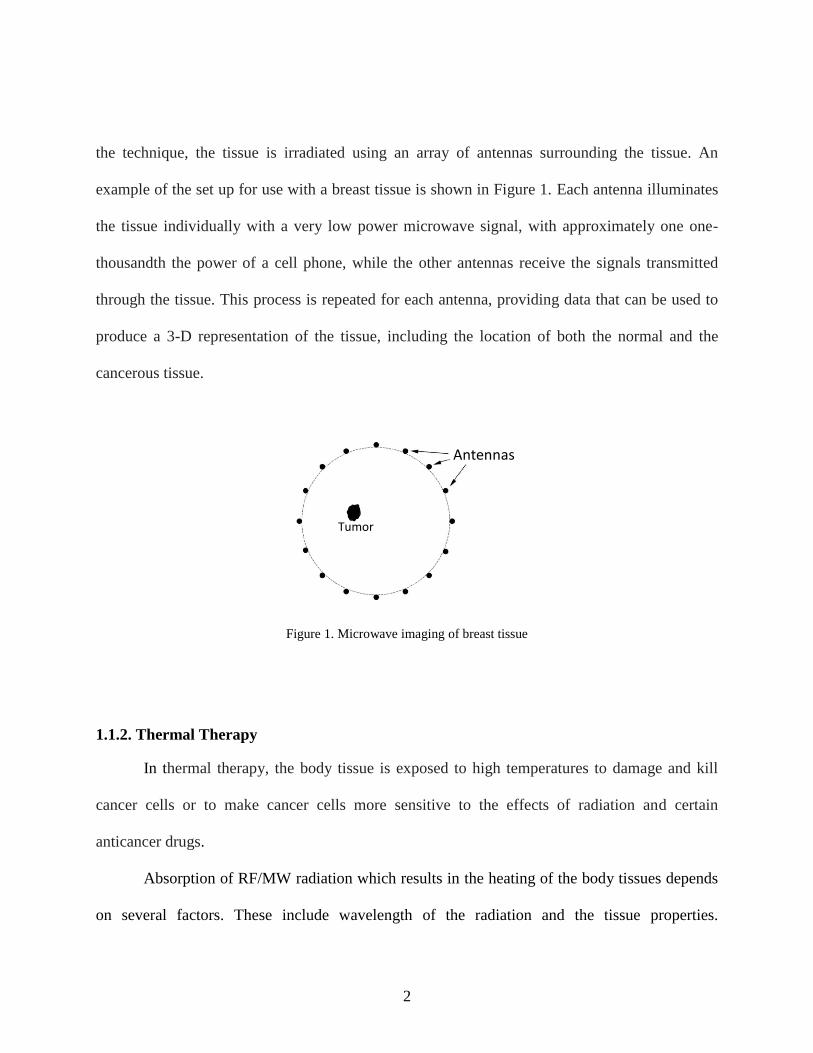
the technique, the tissue is irradiated using an array of antennas surrounding the tissue. An
example of the set up for use with a breast tissue is shown in Figure 1. Each antenna illuminates
the tissue individually with a very low power microwave signal, with approximately one one-
thousandth the power of a cell phone, while the other antennas receive the signals transmitted
through the tissue. This process is repeated for each antenna, providing data that can be used to
produce a 3-D representation of the tissue, including the location of both the normal and the
cancerous tissue.
Figure 1. Microwave imaging of breast tissue
1.1.2. Thermal Therapy
In thermal therapy, the body tissue is exposed to high temperatures to damage and kill
cancer cells or to make cancer cells more sensitive to the effects of radiation and certain
anticancer drugs.
Absorption of RF/MW radiation which results in the heating of the body tissues depends
on several factors. These include wavelength of the radiation and the tissue properties.
Antennas
Tumor

3
Frequencies greater than 10,000 MHz (10 GHz) are absorbed mostly in the outer skin.
Frequencies between 10,000 MHz and 2500 MHz penetrate more deeply, approximately 3 mm to
2 cm into the tissue. Frequencies of 2500 MHz to 1300 MHz penetrate deep enough to cause
damage to internal organs by overheating of the tissue [4].
There are a growing number of clinical applications of thermal therapy that benefit
patients with a variety of diseases, such as hyperthermia and thermal ablation.
Hyperthermia: In the late 1950s, it was determined that raising the tumor to temperatures
of 42 - 45 C made them more sensitive to radiation/chemotherapy. This technique has been
proven effective over the past 20 years through clinical trials. The combination of hyperthermia
with radiation therapy has been shown to and improve treatment efficacy, tumor response and
duration of local tumor control. Hyperthermia has been proven successful in the treatment of
recurrent chest wall breast cancer, melanoma, locally advanced head and neck cancer, and
several other cancers. Today, in some countries such as The Netherlands and Germany,
hyperthermia is part of standard cancer care.
Thermal ablation: In this treatment the tissue is destroyed by localized heating or
freezing. Various energy sources including laser, ultrasound and microwaves are found to be
minimally invasive, and potentially useful for this therapy.
Today, according the Society for Thermal Medicine, about 100,000 patients with cancers
of the liver, lung, kidney and bone are annually treated worldwide using thermal therapy, as it
provides local tumor control with minimal side effects. About a dozen FDA approved devices
are available, with novel devices in the pipeline [5]. In addition, the combination of thermal
4
ablation with chemo- or radiation therapy, and immunotherapy, is being pursued in clinical trials
[6, 7].
1.2. Motivation for the Research
Cancer remains one of the leading causes of death in the world. New methods for
treatment of cancer that have been implemented have been successful, but the results are still
limited. The use of hyperthermia along with conventional cancer treatment such as
chemotherapy and radiation has been successful in many cancer treatments [6, 7]. In this
approach, the cancerous tumors are heated to a temperature between 40 and 45°C for a specific
period of time which renders tumor cells more sensitive to radiation and chemotherapy. The
increase in temperature stimulates blood flow in the tumor, increases oxygenation and hence
makes the treatment more effective. High temperatures can kill cancer cells, but they also can
injure or kill normal cells and tissues. Temperatures above 42°C can cause burns and blisters in
healthy tissue. Consequentially, during hyperthermia treatment, the temperature in the tumor and
healthy tissue has to be closely monitored.
In hyperthermia, suitable applicators (antennas) are used to provide energy to penetrate
the body tissues. A majority of the applicators provide good energy deposition in superficial
tumors [8, 9]. For treating deep seated tumors, the frequency of the applicators is lower, and
typically and array of applicators is used as a single applicator may not provide the necessary
energy. With the hyperthermia systems developed for regional hyperthermia of deep seated
tumors, selective heating of those regions is still very difficult. Moreover, in almost all clinical
trials patients experienced local pain and discomfort and the temperature in healthy tissues was
also high [10].
5
The main concern in deep hyperthermia is the power deposition in tumors and the
temperature monitoring during treatment. The current procedures have a limitation on the body
target sites that are too difficult to treat. There is a large need for alternative effective options in
hyperthermia for providing deep seated power deposition various regions of the body, without
affecting healthy surrounding tissues and organs.
Hence, in this research we investigate an enhanced hyperthermia treatment through the
use of magnetic nanoparticles.
1.3. Dissertation Outline
This dissertation consists of 7 major sections. The first chapter is an overview of the use
of high frequency in medicine. It introduces the hyperthermia cancer treatment and the
motivation for this research.
Chapter 2 covers the biological and physical aspects of hyperthermia. The biological
aspects of hyperthermia refers to the electromagnetic propagation in biological tissues and the
physical aspects cover the applicators used in hyperthermia treatments.
Chapter 3 explains in detail the heat transfer in microwave hyperthermia using the
bioheat equation and study the specific absorption rate.
Chapter 4 details the use of magnetic nanoparticles in hyperthermia. The nanoparticle
targeting mechanisms and the heat generated by using nanoparticles during hyperthermia
treatment are presented.
6
Chapter 5 focuses on a primary study of microwave hyperthermia in breast cancer
treatment using magnetic nanoparticles. The results of simulation and measurement are included
in this chapter.
Chapter 6 presents results for an enhanced hyperthermia treatment for liver cancer with
realistic human models incorporating the blood perfusion rate. Here, the results of simulations
and measurement are presented.
Conclusions of this research are presented in Chapter 7.

7
CHAPTER 2: BIOLOGICAL AND PHYSICAL ASPECTS OF
HYPERTHERMIA
2.1. RF/Microwave Propagation in Biological Tissues
The interaction of the high frequency fields with the biological tissues is determined to a
large extent by the characteristics of the tissue permittivity , permeability and conductivity .
Biological tissues are non-magnetic and hence the permeability does not play a major role.
There are several sources in the literature [11, 12] where the , and values for various tissues
such as muscles, bone, blood, liver, kidney, etc., at various frequencies are provided. Table 1
shows the dielectric properties of human tissues at 3 different frequencies 915 MHz, 2.45 GHz
and 10 GHz. Heat absorption will be greatest in tissues that have high water content, such as
muscle, with less heat absorption taking place in bone and fat [12].
2.2. Electromagnetic Waves Propagating in Biological Tissues
When the biological tissues are exposed to RF/Microwave radiation, the characteristics of
the tissues will determine the amount of energy reflected by or absorbed in the tissue.
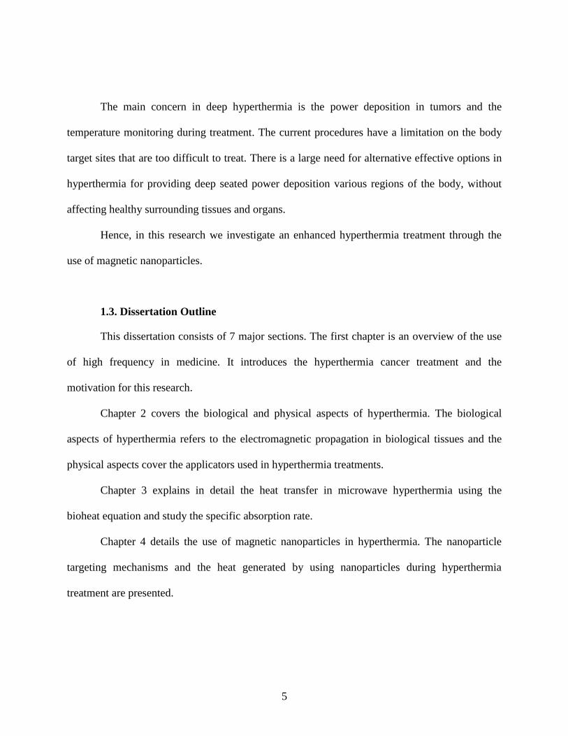
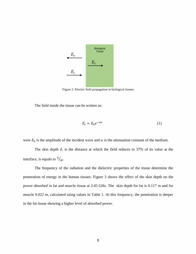
Consider a tissue with an incident linearly polarized EM wave propagating along z
direction, as shown in Figure 2, with its E field polarized along x direction and H field polarized
along y direction. 𝐸𝑖 is the incident electric field, 𝐸𝑡 is the transmitted electric field and 𝐸𝑟 is the
reflected electric field.
8
Figure 2. Electric field propagation in biological tissues
The field inside the tissue can be written as:
𝐸𝑡 = 𝐸0𝑒−𝛼𝑧 (1)
were 𝐸0 is the amplitude of the incident wave and is the attenuation constant of the medium.
The skin depth 𝛿, is the distance at which the field reduces to 37% of its value at the
interface, is equals to 1 𝛼⁄ .
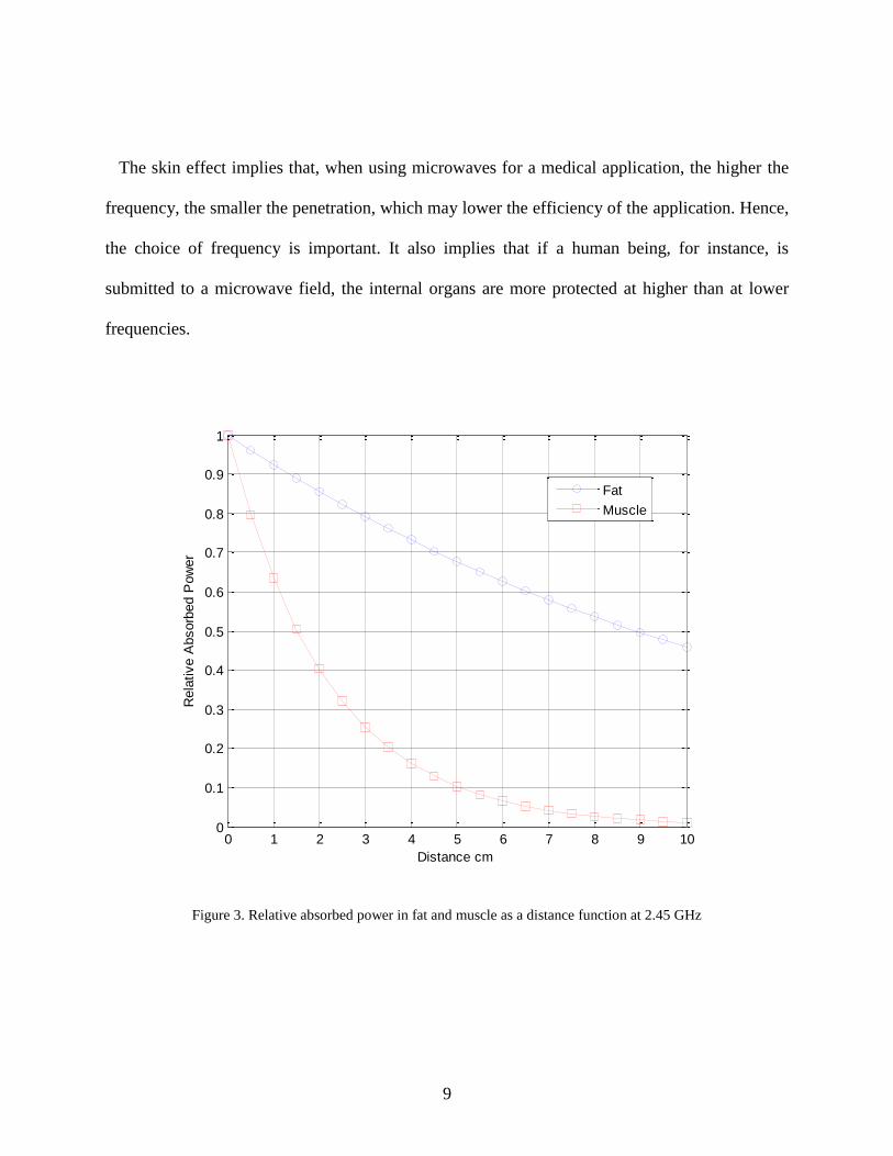
The frequency of the radiation and the dielectric properties of the tissue determine the
penetration of energy in the human tissues. Figure 3 shows the effect of the skin depth on the
power absorbed in fat and muscle tissue at 2.45 GHz. The skin depth for fat is 0.117 m and for
muscle 0.022 m, calculated using values in Table 1. At this frequency, the penetration is deeper
in the fat tissue showing a higher level of absorbed power.
Biological Tissue
𝐸𝑖
𝐸𝑡
𝐸𝑟
9
The skin effect implies that, when using microwaves for a medical application, the higher the
frequency, the smaller the penetration, which may lower the efficiency of the application. Hence,
the choice of frequency is important. It also implies that if a human being, for instance, is
submitted to a microwave field, the internal organs are more protected at higher than at lower
frequencies.
Figure 3. Relative absorbed power in fat and muscle as a distance function at 2.45 GHz
0 1 2 3 4 5 6 7 8 9 100
0.1
0.2
0.3
0.4
0.5
0.6
0.7
0.8
0.9
1
Distance cm
Rela
tive A
bsorb
ed P
ow
er
Fat
Muscle

10
Table 1. Dielectric properties of human tissues at different frequencies
915 MHz 2.45 GHz
Tissue Name
Conductivity Relative Loss Conductivity Relative Loss
[S/m] permittivity tangent [S/m] permittivity tangent
Bladder 0.38506 18.923 0.39976 0.68532 18.001 0.27933
Blood 1.5445 61.314 0.49487 2.5448 58.264 0.32046
Blood Vessel
0.70087 44.741 0.30774 1.4353 42.531 0.2476
Bone Cancello
0.34353 20.756 0.32515 0.80517 18.548 0.31849
Bone Cortical
0.14512 12.44 0.22919 0.39431 11.381 0.2542
Bone Marrow
0.040588 5.5014 0.14494 0.095037 5.2969 0.13164
Breast Fat 0.049523 5.4219 0.17944 0.13704 5.1467 0.19535
Cartilage 0.7892 42.6 0.36394 1.7559 38.77 0.33228
Colon 1.087 57.867 0.36901 2.0383 53.879 0.27757
Cornea 1.4008 55.172 0.49878 2.2954 51.615 0.32629
Fat 0.051402 5.4596 0.18496 0.10452 5.2801 0.14524
GallBladder 1.2614 59.118 0.41918 2.059 57.634 0.26212
Heart 1.2378 59.796 0.40668 2.2561 54.814 0.30199
Kidney 1.4007 58.556 0.46991 2.4295 52.742 0.33797
Liver 0.86121 46.764 0.36179 1.6864 43.035 0.28751
Muscle 0.94809 54.997 0.33866 1.7388 52.729 0.24194
Nerve 0.57759 32.486 0.34929 1.0886 30.145 0.26494
Prostate 1.2159 60.506 0.39477 2.1676 57.551 0.27633
Retina 1.1725 55.23 0.41706 2.0332 52.628 0.28345
Skin 0.87169 41.329 0.41435 1.464 38.007 0.28262
Small Intestin
2.173 59.389 0.71881 3.1731 54.425 0.42777
Spinal Cord 0.57759 32.486 0.34929 1.0886 30.145 0.26494
Stomach 1.1932 65.02 0.36053 2.2105 62.158 0.36053
Tooth 0.14512 12.44 0.22919 0.39431 11.381 0.2542
11
The amount of power deposition in the body is be expressed through the specific
absorption rate (SAR), measured in watts per kilogram of mass tissue and is a simple and useful
value for quantifying the interactions of RF/microwave radiation with living systems. The SAR
is defined as the ratio of the total power absorbed in the exposed body to the mass in which it is
absorbed, which is not necessarily that of the total body:
𝑆𝐴𝑅 =𝜎𝐸2
𝜌 (2)
where E is the root mean square electric field [V/m], is the conductivity [S/m], and is the
mass density of the tissue [kg/m3].
2.3. Hyperthermia
The normal temperature in a human body is 37°C. Hyperthermia refers to increase in the
normal temperature in the human body. In hyperthermia treatment, cancerous cells temperatures
are elevated to the range between 42 - 45°C, so as to destroy them. This treatment can be done
without substantial damage to healthy tissues and with minimal side effects. Hyperthermia
cancer treatment is been used nowadays in combination with radiotherapy and chemotherapy.
Hyperthermia can be used to treat specific tumor locations or for the entire body. In local
hyperthermia, used to increase the temperature in a specific area that contains a tumor, the heat
generation can be achieved by external applicators to treat tumors near the skin’s surface or with
probes to reach deep-seated cancerous tissues. Regional hyperthermia is used for larger or
12
multiple tumor locations or to treat cancers that have spread to several regions. Here, a larger
part of the body is heated to destroy the cancerous cells [13, 14]. This treatment is also usually
combined with chemotherapy or radiation therapy.
In hyperthermia treatment, the high frequency electromagnetic energy is applied to the
tissue using either external or internal applicators depending on the tumor location. Internal
applicators use a needle or probe to release the energy directly into the tumor, and external
applicators radiate the tissue from outside.
Healthy tissues can also absorb electromagnetic energy and get heated leading to burns,
blisters, and discomfort. Thus, it is critical to monitor temperatures in healthy tissues during
hyperthermia treatment.
2.4. Hyperthermia Applicators
Electromagnetic hyperthermia used before the 1950s was not well developed and mainly
empirical [15, 16]. After 1950, hyperthermia as a separate treatment modality started [17].
Research work was focused on the development of quasi-static or radiative techniques using
electromagnetic energy. Initially, these devices operated only at the ISM (Industry Science and
Medicine) frequencies, and typically had a single power source, one applicator and limited
treatment area. Electric and magnetic field were used to deliver the electromagnetic energy to the
patient through the air. Over the years, various applicators were developed to provide better
tissue deposition and maintain heterogeneous skin cooling. In addition, several advanced
computer aided design allowed the design of efficient applicators [18-22].

13
2.4.1. Inductive Heating
For inductive heating, an inductive concentric coil is placed around the patient avoiding
contact between the patient and the applicator. The electromagnetic energy is transferred through
magnetic fields. It was found that one main disadvantage of these devices is that the power
deposition at the center of the target tissue is very low [23].
In order to solve this problem, a helical coil applicator with a coaxial pair magnetic
system was developed [24]. This device creates homogeneous energy deposition in the patient by
moving the applicator around its longitudinal axis. It operates at its resonance frequency and
creates eddy currents by the inductive field component. However, this device had limited spatial
control of the energy deposition and the blood perfusion played an important role in the tumor
heating.
2.4.2. Capacitive Heating
Here, the electric field is used to transfer the electromagnetic energy to the tissue, with
one electrode placed below and one above the patient [25]. The energy deposition depends on the
sizes of electrodes and the electric field. It is seen that there is a high power deposition in the
subcutaneous fatty tissue. The disadvantages of this devices is that the energy distribution will
depend only on the electrodes position and size and hence the treatment needs to be stopped to
make any change in electrodes. The blood perfusion plays and important role in the tumor
heating [25].
14
2.4.3. Radiation Heating
Cylindrical waveguides and dipole antennas are used as radiating devices for radiation
heating [26]. The main disadvantage with these applicators is that the volume treated is very
small and the antennas used have low directivity. The radiating elements are divided into devices
for use in superficial hyperthermia and for deep hyperthermia, based on the frequency and tumor
location.
When the tumors are superficial, less number of applicators are needed. Multi-elements
applicators are used to obtain a high heterogeneity of SAR distribution [27-30].
2.4.4. Interstitial Applicators
The electromagnetic energy can also be delivered to the diseased tissue through an
invasive process where antennas (needles) are inserted into the tumor. These are placed inside
the patient using imaging guidance, such as CT (computed tomography) or ultrasound. These
applicators can also be used during an open surgical procedure to target and ablate the diseased
soft-tissue [31].
Due to the invasive nature of this technique, these applicators can cause discomfort and
complications prior to, during and after each treatment.
15
CHAPTER 3: HEAT TRANSFER IN HYPERTHERMIA
3.1. Introduction
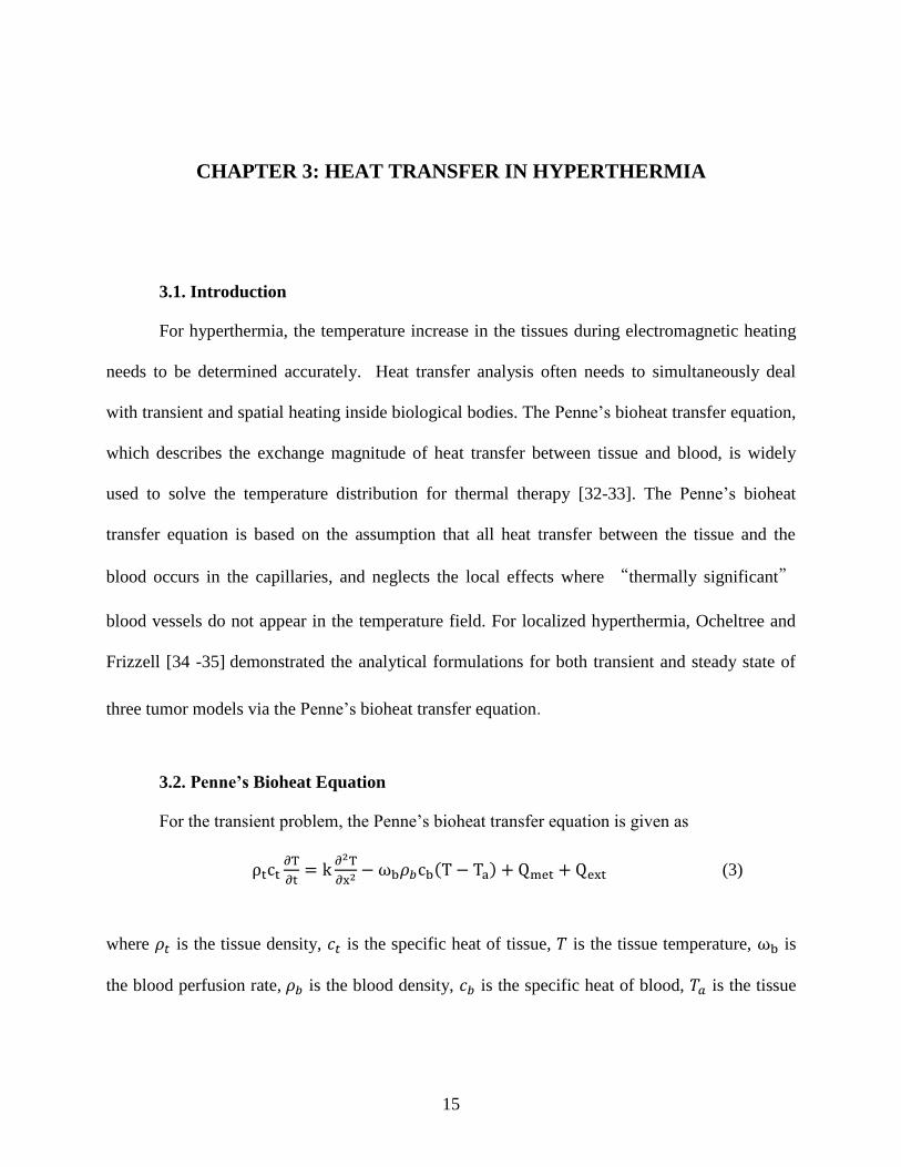
For hyperthermia, the temperature increase in the tissues during electromagnetic heating
needs to be determined accurately. Heat transfer analysis often needs to simultaneously deal
with transient and spatial heating inside biological bodies. The Penne’s bioheat transfer equation,
which describes the exchange magnitude of heat transfer between tissue and blood, is widely
used to solve the temperature distribution for thermal therapy [32-33]. The Penne’s bioheat
transfer equation is based on the assumption that all heat transfer between the tissue and the
blood occurs in the capillaries, and neglects the local effects where “thermally significant”
blood vessels do not appear in the temperature field. For localized hyperthermia, Ocheltree and
Frizzell [34 -35] demonstrated the analytical formulations for both transient and steady state of
three tumor models via the Penne’s bioheat transfer equation.
3.2. Penne’s Bioheat Equation
For the transient problem, the Penne’s bioheat transfer equation is given as
ρtct∂T
∂t= k
∂2T
∂x2 − ωb𝜌𝑏cb(T − Ta) + Qmet + Qext (3)
where 𝜌𝑡 is the tissue density, 𝑐𝑡 is the specific heat of tissue, 𝑇 is the tissue temperature, ωb is
the blood perfusion rate, 𝜌𝑏 is the blood density, 𝑐𝑏 is the specific heat of blood, 𝑇𝑎 is the tissue

16
temperature, 𝑘 is the thermal conductivity of tissue, 𝑄𝑚𝑒𝑡 is the heat coming from metabolism,
𝑄𝑒𝑥𝑡is the absorbed power due to an external source and can be written as:
𝑄𝑒𝑥𝑡 =1
2𝜎𝑡|𝐸|2 (4)
where 𝜎𝑡 is the electrical conductivity of the tissue and E is the electric field generated by the
EM applicator. By analyzing (4), it is evident that only the E field is taken into account to obtain
the temperature increase in tissues and tumors. Although the EM applicator generates E and H
fields, the effect of the H field is neglected because biological tissues are nonmagnetic.
3.3. Specific Absorption Rate (SAR)
The specific absorption rate (SAR) is a measure of the energy absorbed by the tissue due
to electromagnetic radiation and is related to the increase in temperature in the tissue. The SAR
is the ratio of the total power absorbed in the exposed body to the mass in which it is absorbed,
as explained in Section 2.2. The amount of energy absorbed by the tissue depends on several
factors including frequency, dielectric property of the tissue, irradiating time exposure, intensity
of electromagnetic radiation, and water content of the tissue.
As exposure to high frequency electromagnetic radiation can cause damage to tissues,
there are strict safety guidelines for exposure that are set by the Federal Communications
Commission FCC [36, 37].
In sensitive organs, small temperature increases can produce severe physiological effects.
An increase of approximately 1–5°C in human body temperature can cause numerous
17
malformations, temporary infertility in males, brain lesions, and blood chemistry changes. Even
a small temperature increase in human body (approximately 1°C) can lead to altered production
of hormones and suppressed immune response [36].
At high frequencies human tissues with finite electric conductivity are generally lossy
mediums and are usually neither good dielectric materials nor good conductors and as
electromagnetic waves propagate through the human tissues, the energy of EM waves is
absorbed by the tissues.
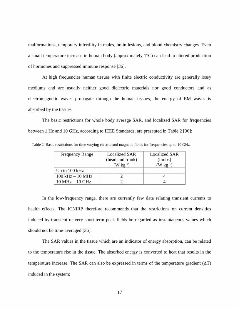
The basic restrictions for whole body average SAR, and localized SAR for frequencies
between 1 Hz and 10 GHz, according to IEEE Standards, are presented in Table 2 [36]:
Table 2. Basic restrictions for time varying electric and magnetic fields for frequencies up to 10 GHz.
Frequency Range Localized SAR
(head and trunk)
(W kg-1)
Localized SAR
(limbs)
(W kg-1)
Up to 100 kHz - -
100 kHz – 10 MHz 2 4
10 MHz – 10 GHz 2 4
In the low-frequency range, there are currently few data relating transient currents to
health effects. The ICNIRP therefore recommends that the restrictions on current densities
induced by transient or very short-term peak fields be regarded as instantaneous values which
should not be time-averaged [36].
The SAR values in the tissue which are an indicator of energy absorption, can be related
to the temperature rise in the tissue. The absorbed energy is converted to heat that results in the
temperature increase. The SAR can also be expressed in terms of the temperature gradient (T)
induced in the system:
18
𝑆𝐴𝑅 = 𝑐∆𝑇
∆𝑡 (5)
where 𝑐 is the specific heat of the tissue and ∆𝑡 is the treatment time. This definition relates the
temperature changes in the tissue to the SAR values in the tissue.
19
CHAPTER 4: MAGNETIC FLUID HYPERTHERMIA
4.1. Introduction
Nanoparticles are microscopic particles with dimensions of less than 100 nm. They
possess a wide variety of potential applications and are now used for medical diagnosis and for
treatment. Fluorescent semiconductor nanoparticles, known as quantum dots, are used for
imaging of biological entities [38] and superparamagnetic nanoparticles are used as contrast
agents for magnetic resonance imaging (MRI) to help diagnose various diseases [39].
The multifunctional characteristic of nanoparticles makes them great candidates for
targeted drug delivery and cancer treatment, and they are currently in use as anti-cancer drug and
gene carriers for controlling cancer [40].
For cancer therapy, the nanoparticle distribution within the body depends on various
parameters such as their relatively small size resulting in longer circulation times and their ability
to take advantage of tumor characteristics. For example, nanoparticles less than 20 nm in size are
able to pass through blood vessel walls and such small particle size allows for intravenous
injection as well as intramuscular and subcutaneous applications. The small size of the
nanoparticles minimizes the irritant reactions at the injection site as compared to conventional
cancer treatments. Furthermore, nanoparticle size allows for interactions with biomolecules on
the cell surfaces and within the cells without altering the behavior and biochemical properties of
those molecules [41].
Nanoparticles can be formulated for specific uptake within the body and for a specific
response by the body to cancer treatment. Nanoparticles can be formulated from a variety of

20
materials so as to carry substances in a controlled and targeted manner. Synthetic polymers,
which are bio-degradable, are used to prepare the nanoparticles for drug delivery. In
transportation, this prevents degradation of the carried load and also protects transported
substances from contact with healthy tissues, hence reducing side effects and increasing the
relative amount of the load reaching the diseased tissue.
4.2. Nanoparticle Targeting
In treatments using nanoparticles, the goal is to have them reach the desired tumor sites,
after administration, with minimal loss to their volume and activity in blood circulation and to
attach to tumor cells without harmful effects to healthy tissue. This may be achieved using two
strategies: passive and active targeting of drugs.
Passive drugs targeting consists in the transport of nanoparticles through tumor
capillaries by convection or passive diffusion [42]. Tumor vessels are highly disorganized and
dilated with a high number of pores, resulting in enlarged gap junctions between endothelial cells
and compromised lymphatic drainage. In this case, nanoparticles may be released in the
extracellular matrix and then diffused through the tumor tissue.
In active targeting, targeting ligands are attached at the surface of the nanoparticle for
binding to appropriate receptors expressed at the tumor site. The ligand is chosen to bind to a
receptor of specific tumor cells and not expressed by normal cells [42].
4.3. Heat Generation of Nanoparticles
When nanoparticles are exposed to an electromagnetic field, they transform the energy of
the electromagnetic field into heat by different mechanisms. This transformation depends on the
21
frequency of the external field and on the characteristics of the particles such as their size and
other characteristics [43 – 45].
4.3.1. Hysteresis
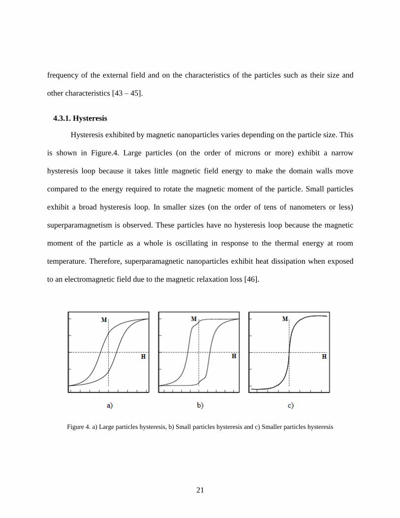
Hysteresis exhibited by magnetic nanoparticles varies depending on the particle size. This
is shown in Figure.4. Large particles (on the order of microns or more) exhibit a narrow
hysteresis loop because it takes little magnetic field energy to make the domain walls move
compared to the energy required to rotate the magnetic moment of the particle. Small particles
exhibit a broad hysteresis loop. In smaller sizes (on the order of tens of nanometers or less)
superparamagnetism is observed. These particles have no hysteresis loop because the magnetic
moment of the particle as a whole is oscillating in response to the thermal energy at room
temperature. Therefore, superparamagnetic nanoparticles exhibit heat dissipation when exposed
to an electromagnetic field due to the magnetic relaxation loss [46].
Figure 4. a) Large particles hysteresis, b) Small particles hysteresis and c) Smaller particles hysteresis
22
4.3.2. Relaxation
The heat dissipation of superparamagnetic nanoparticles is due to the delay in relaxation
of the magnetic moment. This relaxation can correspond either to the physical rotation of the
particles themselves within the fluid, known as Brownian relaxation, or the rotation of the
magnetic moments within each particle known as Néel relaxation.
The Brownian 𝜏𝐵 and Néel 𝜏𝑁 relaxation times are given by the following equations:
𝜏𝐵 = 4𝜋𝑟ℎ3/(𝑘𝑇) (6)
τN = τ0exp [KV
kT] (τ0~10−9𝑠) (7)
where is the viscosity of the fluid, T the temperature, and 𝑟ℎ is the hydrodynamic radius which
due to particle coating may be essentially larger than the radius of the magnetic particle core, K
is the anisotropy constant, 𝑉 is the magnetic volume, and 𝜏0 = 10−9 𝑠. Since Brownian and Néel
relaxation processes occur in parallel, the effective relaxation time is given by:
1
𝜏=
1
𝜏𝐵+
1
𝜏𝑁 (8)
23
The relationship between magnetization M and the applied magnetic field H is expressed
through the magnetic susceptibility , which explains how magnetization varies with the applied
magnetic field:
M = H (9)
The Brownian relaxation time is related to the applied magnetic field through the
complex magnetic susceptibility and can be obtained from the following equation [45]:
(𝑓) =0
1−𝑖2𝑓𝐵 (10)
where
0 is the equilibrium susceptibility
The shorter relaxation time term dominates the effective relaxation time for a given
particle size. 𝜏𝐵 is determined in part by the hydrodynamic properties of the fluid, while 𝜏𝑁 is
governed by the magnetic anisotropy energy relative to thermal energy. Both Brownian and Néel
processes may be present in a ferrofluid. In constrained (i.e., immobilized) superparamagnetic
particles, such as iron oxide, only Néel relaxation occurs.
Relaxation times are temperature dependent. However for mild hyperthermia at near
42ºC, the relaxation time constants do not change by much, thus in this investigation the effect of
small temperature elevations on the time constants are considered negligible.
The real and imaginary parts of the complex susceptibility can be expressed as shown in
(11) and (12) [45]:
24
′ =0
1+(𝜔𝜏)2 (11)
′′ =𝜔𝜏
1+(𝜔𝜏)2
0 (12)
where 𝜔 = 2𝑓, 𝜏 is the relaxation time. 0 is the equilibrium susceptibility, and can be
calculated from the following expressions:
0
= 𝑖
3
(𝑐𝑜𝑡ℎ −
1
) (13)
where the initial susceptibility 𝑖 is:
𝑖
= 𝜇0∅𝑀𝑑
2𝑉𝑀
3𝑘𝐵𝑇 (14)
and is the Langevin equation expressed as:
=𝜇0𝑀𝑑
2𝐻0𝑉𝑀
𝑘𝐵𝑇 (15)
where ∅ is the volume fraction of nanoparticles in the ferrofluid and 𝑀𝑑 is the domain
magnetization of the nanoparticle, 𝐻0 is the initial magnetic field, 𝑉𝑀 is the volume of
nanoparticle and 𝑘𝐵 is the Boltzmann constant [45].
25
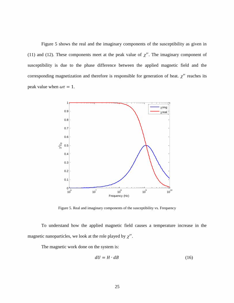
Figure 5 shows the real and the imaginary components of the susceptibility as given in
(11) and (12). These components meet at the peak value of ′′. The imaginary component of
susceptibility is due to the phase difference between the applied magnetic field and the
corresponding magnetization and therefore is responsible for generation of heat. ′′ reaches its
peak value when 𝜔𝜏 = 1.
Figure 5. Real and imaginary components of the susceptibility vs. Frequency
To understand how the applied magnetic field causes a temperature increase in the
magnetic nanoparticles, we look at the role played by ′′.
The magnetic work done on the system is:
𝑑𝑈 = 𝐻 ∙ 𝑑𝐵 (16)
106
107
108
109
1010
0
0.1
0.2
0.3
0.4
0.5
0.6
0.7
0.8
0.9
1
/
0
Frequency (Hz)
img
real
26
where 𝐻 (𝐴/𝑚−1) is the magnetic field intensity and 𝐵(𝑇) the induction. The fields are collinear
and 𝐻 snd 𝐵 are magnitudes. Then, the relation between the magnetic field 𝐻 (𝐴/𝑚) and the
magnetic flux density (or induction flux) 𝐵 (𝑊𝑏/𝑚2), is:
𝐵 = 𝜇0(𝐻 + 𝑀) (17)
where 𝜇0 is the permeability of free space and 𝑀 is the magnetization of the material (Am-1) .
When the magnetization lags the field, the integration yields a positive result indicating
conversion of magnetic work to internal energy [45], which can be expressed as:
∆𝑈 = −𝜇0 ∮ 𝑀𝑑𝐻 (18)
where ∆𝑈 is the internal energy.
From (9), the magnetization as a function of time becomes:
𝑀(𝑡) = 𝑅𝑒[𝐻0𝑒𝑖𝜔𝑡] = 𝐻0(′ cos(𝜔𝑡) + ′′ sin(𝜔𝑡)) (19)
where it is seen that ′ is the in-phase component, and ′′ the out-of-phase component of
and the internal energy can be expressed as:
∆𝑈 = 𝜇0𝐻02′′ ∫ 𝑠𝑖𝑛2(𝜔𝑡)𝑑𝑡
2𝜋/𝜔
0 (20)
The volumetric power dissipation can now be expressed as:
27
𝑃 = ∆𝑈𝑓 = 𝜇0𝑓𝐻02𝜔′′ ∫ 𝑠𝑖𝑛2(𝜔𝑡)𝑑𝑡
2𝜋/𝜔
0= 𝜇0𝑓𝐻0
2𝜋′′ (21)
where 𝑓is the frequency.
Hence we see that when magnetic nanoparticles are injected into tumors, their magnetic
properties are intensified, due to the complex susceptibility ′′. Consequently, the external H
field applied also plays an important role in the heating process.
From (21), it is observed that the power dissipation is proportional to the square of the
amplitude of the H field intensity. Therefore, in the bioheat equation (3) written earlier, we
include an additional term in Qext :
ρtct∂T
∂t= k
∂2T
∂x2− 𝜔b𝜌𝑏cb(T − Ta) + Qmet +
1
2𝜎𝑡|𝐸|2 + 𝜋𝜇0
"𝑓|𝐻|2 (22)
With nanoparticles injected into a tumor, the heating effect is produced by both the
electric and magnetic fields generated by the external applicator; i.e., the heating effect produced
by the external applicator in the tumor, depends not only of the square of E field but also of the
square of H field.
When magnetic nanoparticles are present, the relation between the specific absorption
rate (SAR) and the time rate of change of the temperature in the magnetic material is often
expressed as:
𝑆𝐴𝑅 =𝑐𝑉𝑠
𝑚
𝑑𝑇
𝑑𝑡 (23)
28
where 𝑐 is the specific heat capacity of the sample, 𝑚 is the mass of the magnetic particles, 𝑉𝑠 is
the total volume of the tissue containing the nanoparticle and 𝑑𝑇
𝑑𝑡 is the temperature increment.
The specific absorption rate SAR is also proportional to the volumetric power dissipation
P and can be written as:
𝑆𝐴𝑅 = 𝜌 ∗ 𝑃 = 𝜌𝜋𝜇0"𝑓|𝐻|2 (24)
where 𝜌 is the density of nanoparticle.
29
CHAPTER 5: MICROWAVE MAGNETIC FLUID
HYPERTHERMIA MODELING
5.1. Introduction
The results for enhanced magnetic fluid hyperthermia using magnetic nanoparticles is
presented for the case of a tumor in the breast tissue. The mathematical modeling is done using
the Penne’s bioheat equation. Simulations are carried out with HFSS and SEMCAD X [47]. The
SAR values and the transient temperature are studied as a function of the nanoparticle
characteristics, such as size, concentration etc. Experiments on phantoms breast and tumor tissue
were conducted to validate the simulated results obtained.
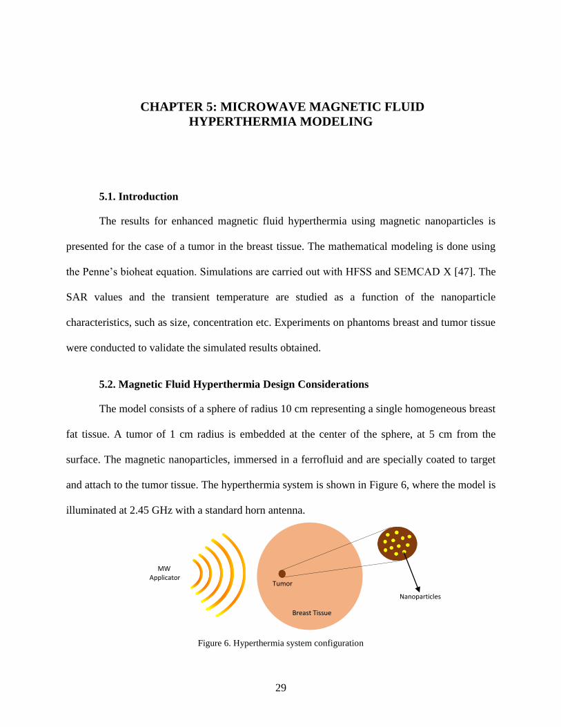
5.2. Magnetic Fluid Hyperthermia Design Considerations
The model consists of a sphere of radius 10 cm representing a single homogeneous breast
fat tissue. A tumor of 1 cm radius is embedded at the center of the sphere, at 5 cm from the
surface. The magnetic nanoparticles, immersed in a ferrofluid and are specially coated to target
and attach to the tumor tissue. The hyperthermia system is shown in Figure 6, where the model is
illuminated at 2.45 GHz with a standard horn antenna.
Figure 6. Hyperthermia system configuration
Tumor
MW Applicator
Nanoparticles
Breast Tissue
30
The electric properties of human breast tissue and tumor tissue such as dielectric constant
and conductivity properties used in the model were assigned according to [12] and the SEMCAD
X software database [47] and [48]. Table 3 lists these values.
Table 3. Electrical properties of human tissues
Tissues 휀𝑟 𝜎 (S/m)
Breast Fat 5.28 0.105
Tumor 60.26 1.21
5.3. Heat Generation
With nanoparticles of concentration 𝑛 and radius 𝑟, the heat generation in tumor will be:
𝑄𝑒𝑥𝑡2 = (4
3𝑛𝜋𝑟3) 𝜋𝜇0
"𝑓|𝐻|2 (25)
where 𝑛 is the concentration of the nanoparticles in tissue, 𝑟 is the radius of the
nanoparticle, " is the magnetic susceptibility and 𝑓 is the frequency.
To determine the transient temperature, as discussed in Chapter 4, the Penne’s bioheat
equation in healthy tissue will be:
ρtct∂T
∂t= k
∂2T
∂x2− ωb𝜌𝑏cb(T − Ta) + Qmet +
1
2𝜎𝑡|𝐸|2
and the Penne’s bioheat equation with nanoparticles in the tumor tissue will be:
ρtct∂T
∂t= k
∂2T
∂x2− ωb𝜌𝑏cb(T − Ta) + Qmet +
1
2𝜎𝑡|𝐸|2 + (
4
3𝑛𝜋𝑟3) 𝜋𝜇0
"𝑓|𝐻|2
The computed heat generation produced by the nanoparticles is included as the heat source
in the bioheat equation to compute the temperature distribution in the model.

31
Table 4 shows the thermal properties considered for healthy and tumor tissues for use in
the bioheat equation, according to [47].
Table 4. Thermal properties of human and tumor tissues
Tissues (kg/m3)
C
(J/kg.C)
K
(W/m.C)
𝑄𝑚𝑒𝑡
(W/kg)
B
(W/m3.C)
Breast Fat 916 2524 0.25 0.328 916
Tumor 1043 3621 0.5 6.807 35
5.4. Simulation
SEMCAD X, a commercial finite-difference time-domain (FDTD) based program for
analysis of bio-electromagnetic effects along with the software HFSS was used to obtain the
SAR values and the transient temperatures. The propagating electromagnetic waves are
generated by an antenna placed near the body with maximum radiation pointing towards the
body. In SEMCAD X, the electric field and magnetic field strengths in the human tissue are
obtained with a sensor called the overall field sensor. SEMCAD X provides thermo-simulation
where the complete thermal profile of human tissues is obtained taking the blood flow, i.e. the
density of blood, blood perfusion rate and the blood specific heat, into account. The program
allows the determination of SAR values and temperature distribution by using thermosensors.
Several thermosensors can be placed along the model to record the temperature. For the
enhanced hyperthermia study in this model the blood flow was not taken into account.
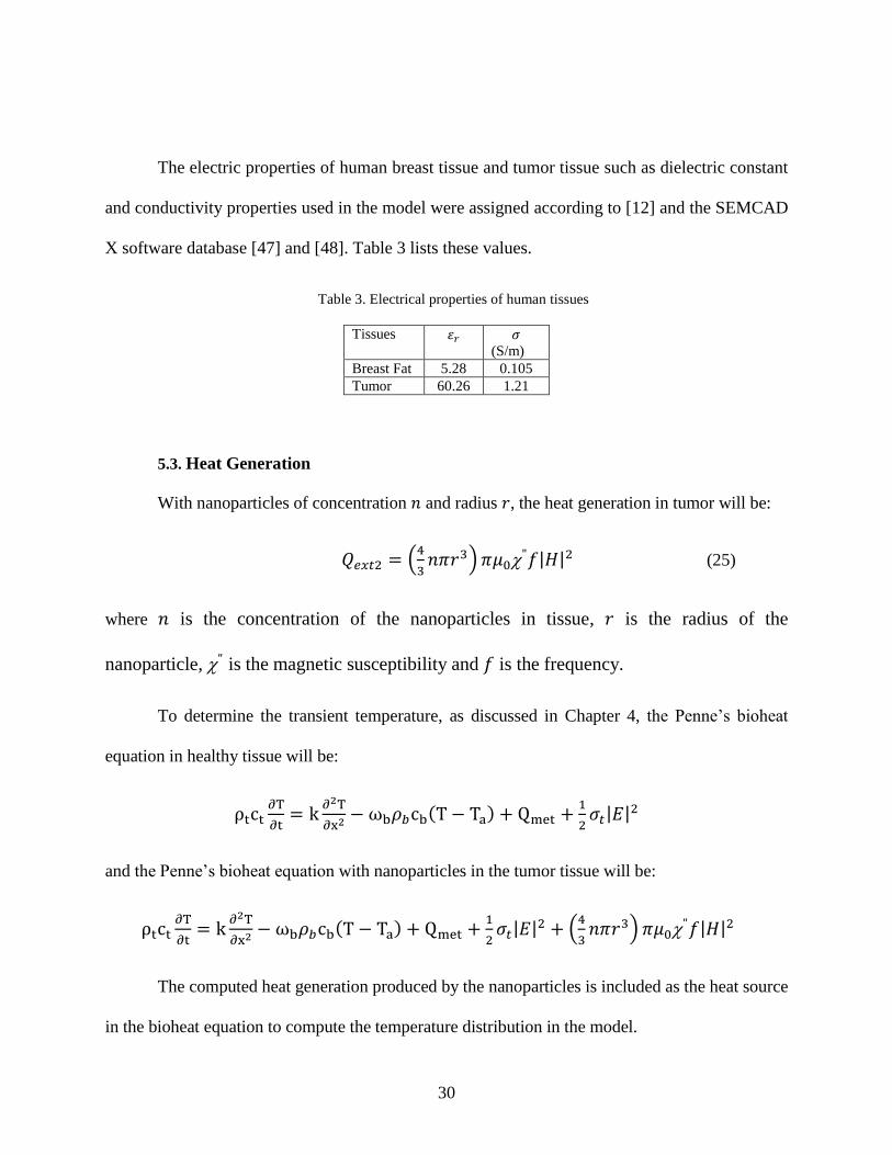
The specific absorption rate and the temperature profile in the model were first evaluated
without injecting any nanoparticles into the tumor. The electromagnetic source was set to 50 V
32
and a tumor of 1 cm was located inside the breast phantom at a depth of 50 mm. the total
treatment time is 1800 sec. The model used in SEMCAD X is shown in Figure 7.
Figure 7. Breast tissue model in SEMCAD X
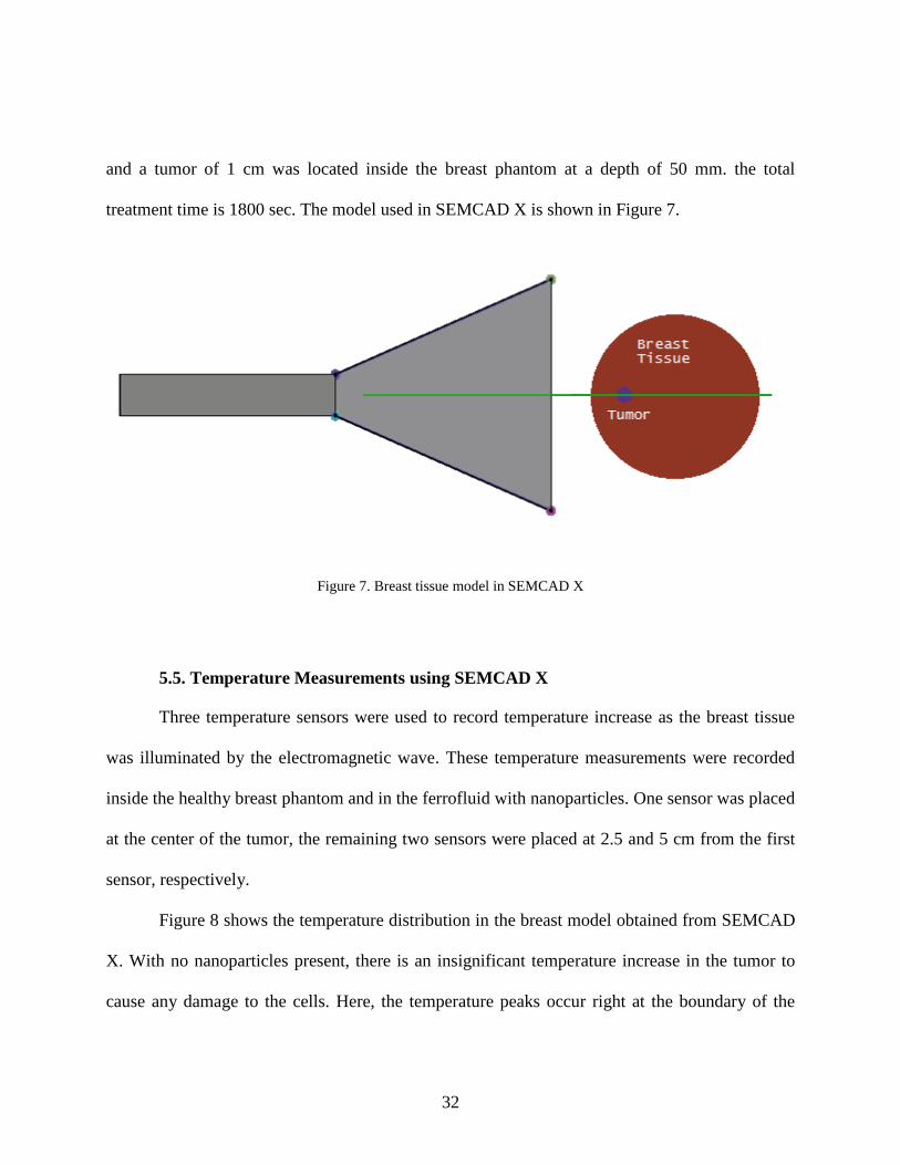
5.5. Temperature Measurements using SEMCAD X
Three temperature sensors were used to record temperature increase as the breast tissue
was illuminated by the electromagnetic wave. These temperature measurements were recorded
inside the healthy breast phantom and in the ferrofluid with nanoparticles. One sensor was placed
at the center of the tumor, the remaining two sensors were placed at 2.5 and 5 cm from the first
sensor, respectively.
Figure 8 shows the temperature distribution in the breast model obtained from SEMCAD
X. With no nanoparticles present, there is an insignificant temperature increase in the tumor to
cause any damage to the cells. Here, the temperature peaks occur right at the boundary of the
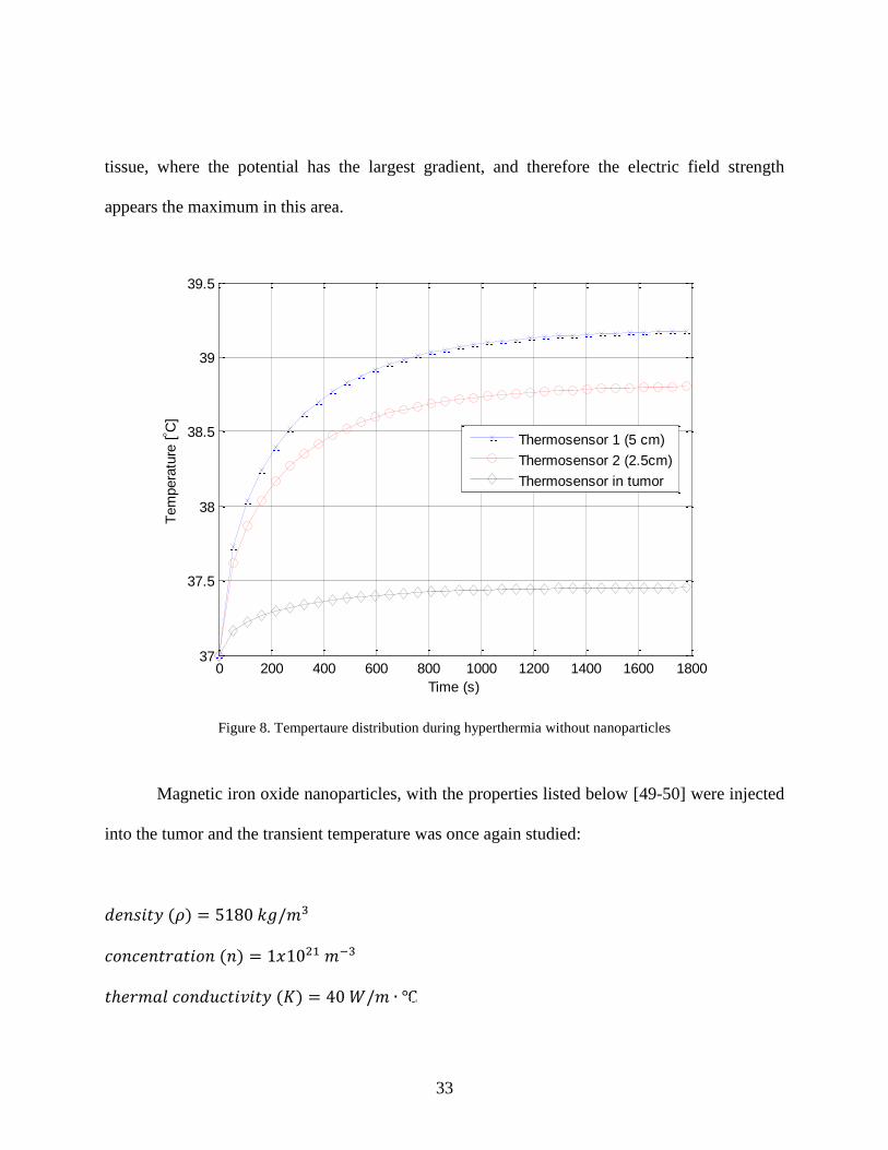
33
tissue, where the potential has the largest gradient, and therefore the electric field strength
appears the maximum in this area.
Figure 8. Tempertaure distribution during hyperthermia without nanoparticles
Magnetic iron oxide nanoparticles, with the properties listed below [49-50] were injected
into the tumor and the transient temperature was once again studied:
𝑑𝑒𝑛𝑠𝑖𝑡𝑦 (𝜌) = 5180 𝑘𝑔/𝑚3
𝑐𝑜𝑛𝑐𝑒𝑛𝑡𝑟𝑎𝑡𝑖𝑜𝑛 (𝑛) = 1𝑥1021 𝑚−3
𝑡ℎ𝑒𝑟𝑚𝑎𝑙 𝑐𝑜𝑛𝑑𝑢𝑐𝑡𝑖𝑣𝑖𝑡𝑦 (𝐾) = 40 𝑊/𝑚 ∙ ℃
0 200 400 600 800 1000 1200 1400 1600 180037
37.5
38
38.5
39
39.5
Time (s)
Tem
pera
ture
[ C
]
Thermosensor 1 (5 cm)
Thermosensor 2 (2.5cm)
Thermosensor in tumor
Tumor
Tumor
34
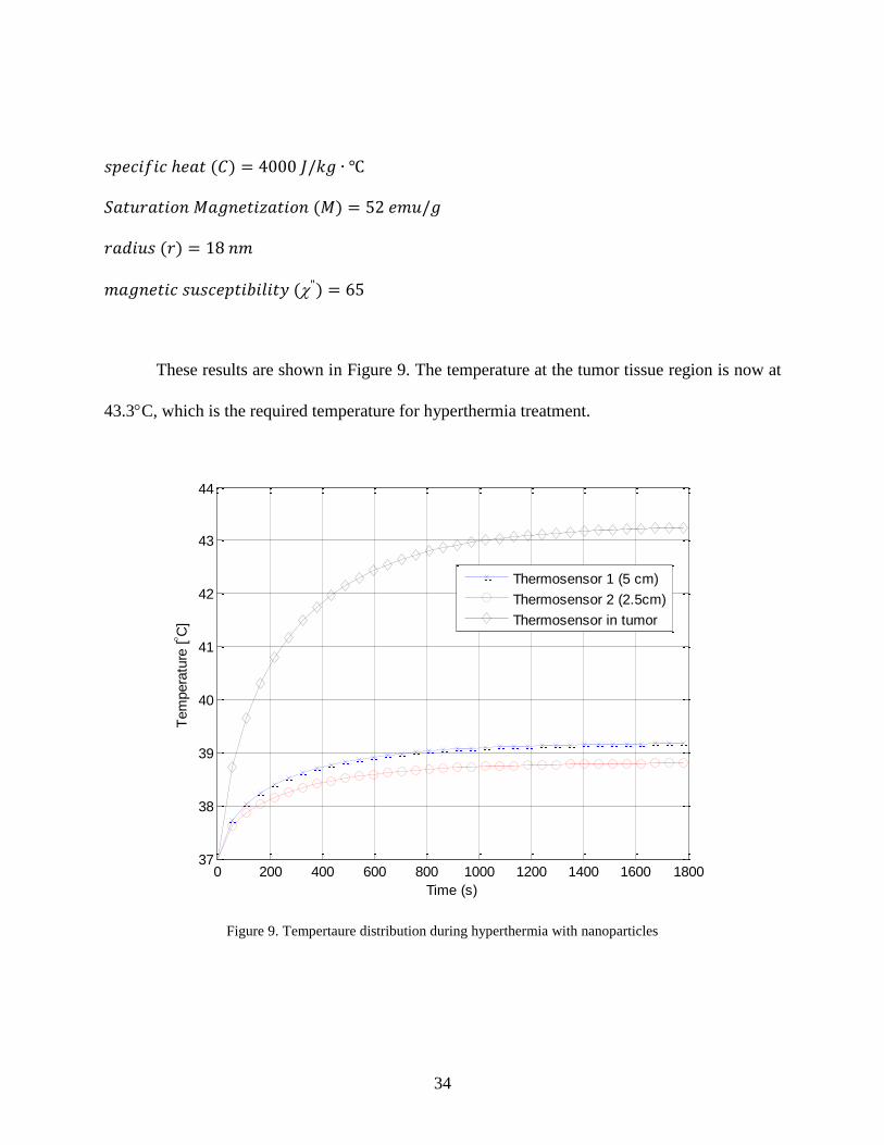
𝑠𝑝𝑒𝑐𝑖𝑓𝑖𝑐 ℎ𝑒𝑎𝑡 (𝐶) = 4000 𝐽/𝑘𝑔 ∙ ℃
𝑆𝑎𝑡𝑢𝑟𝑎𝑡𝑖𝑜𝑛 𝑀𝑎𝑔𝑛𝑒𝑡𝑖𝑧𝑎𝑡𝑖𝑜𝑛 (𝑀) = 52 𝑒𝑚𝑢/𝑔
𝑟𝑎𝑑𝑖𝑢𝑠 (𝑟) = 18 𝑛𝑚
𝑚𝑎𝑔𝑛𝑒𝑡𝑖𝑐 𝑠𝑢𝑠𝑐𝑒𝑝𝑡𝑖𝑏𝑖𝑙𝑖𝑡𝑦 (") = 65
These results are shown in Figure 9. The temperature at the tumor tissue region is now at
43.3C, which is the required temperature for hyperthermia treatment.
Figure 9. Tempertaure distribution during hyperthermia with nanoparticles
0 200 400 600 800 1000 1200 1400 1600 180037
38
39
40
41
42
43
44
Time (s)
Tem
pera
ture
[ C
]
Thermosensor 1 (5 cm)
Thermosensor 2 (2.5cm)
Thermosensor in tumor
35
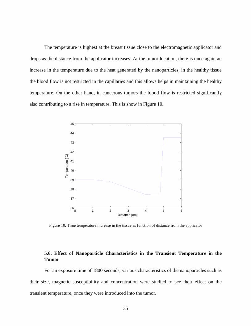
The temperature is highest at the breast tissue close to the electromagnetic applicator and
drops as the distance from the applicator increases. At the tumor location, there is once again an
increase in the temperature due to the heat generated by the nanoparticles, in the healthy tissue
the blood flow is not restricted in the capillaries and this allows helps in maintaining the healthy
temperature. On the other hand, in cancerous tumors the blood flow is restricted significantly
also contributing to a rise in temperature. This is show in Figure 10.
Figure 10. Time temperature increase in the tissue as function of distance from the applicator
5.6. Effect of Nanoparticle Characteristics in the Transient Temperature in the
Tumor
For an exposure time of 1800 seconds, various characteristics of the nanoparticles such as
their size, magnetic susceptibility and concentration were studied to see their effect on the
transient temperature, once they were introduced into the tumor.
0 1 2 3 4 5 636
37
38
39
40
41
42
43
44
45
Distance [cm]
Tem
pera
ture
[ C
]
36
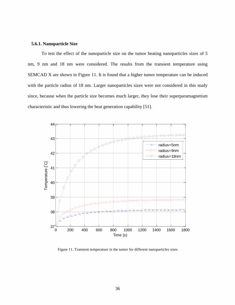
5.6.1. Nanoparticle Size
To test the effect of the nanoparticle size on the tumor heating nanoparticles sizes of 5
nm, 9 nm and 18 nm were considered. The results from the transient temperature using
SEMCAD X are shown in Figure 11. It is found that a higher tumor temperature can be induced
with the particle radius of 18 nm. Larger nanoparticles sizes were not considered in this study
since, because when the particle size becomes much larger, they lose their superparamagnetism
characteristic and thus lowering the heat generation capability [51].
Figure 11. Transient temperature in the tumor for different nanoparticles sizes
0 200 400 600 800 1000 1200 1400 1600 180037
38
39
40
41
42
43
44
Time (s)
Tem
pera
ture
[ C
]
radius=5nm
radius=9nm
radius=18nm
37
Particles with 18 nm diameter showed the highest heating ability obtaining a temperature
rise T = 6 °C and reaching the target temperature of 43.3 °C. The other nanoparticles
considered produced only a temperature raise in the range T= 1 – 3 °C.
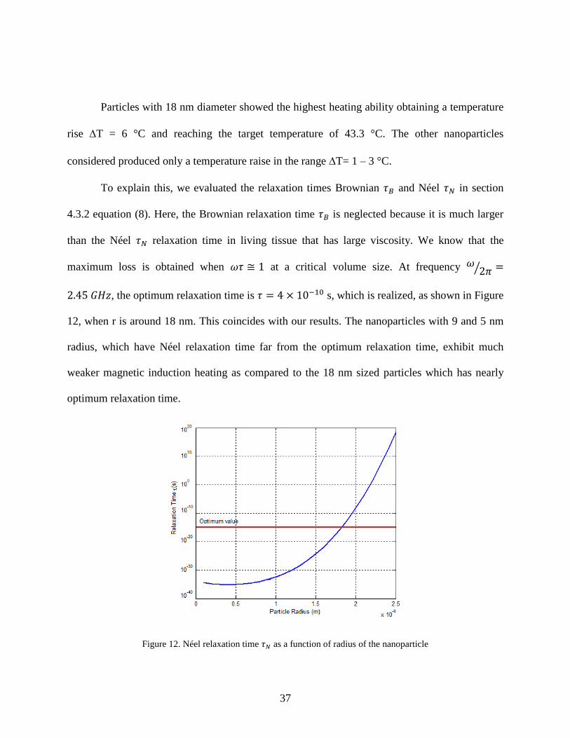
To explain this, we evaluated the relaxation times Brownian 𝜏𝐵 and Néel 𝜏𝑁 in section
4.3.2 equation (8). Here, the Brownian relaxation time 𝜏𝐵 is neglected because it is much larger
than the Néel 𝜏𝑁 relaxation time in living tissue that has large viscosity. We know that the
maximum loss is obtained when 𝜔𝜏 ≅ 1 at a critical volume size. At frequency 𝜔2𝜋⁄ =
2.45 𝐺𝐻𝑧, the optimum relaxation time is 𝜏 = 4 × 10⁻¹⁰ s, which is realized, as shown in Figure
12, when r is around 18 nm. This coincides with our results. The nanoparticles with 9 and 5 nm
radius, which have Néel relaxation time far from the optimum relaxation time, exhibit much
weaker magnetic induction heating as compared to the 18 nm sized particles which has nearly
optimum relaxation time.
Figure 12. Néel relaxation time 𝜏𝑁 as a function of radius of the nanoparticle
38
5.6.2. Nanoparticle Susceptibility
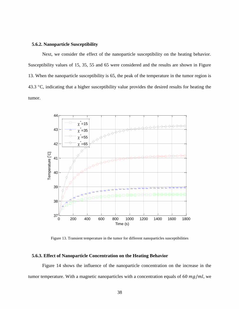
Next, we consider the effect of the nanoparticle susceptibility on the heating behavior.
Susceptibility values of 15, 35, 55 and 65 were considered and the results are shown in Figure
13. When the nanoparticle susceptibility is 65, the peak of the temperature in the tumor region is
43.3 C, indicating that a higher susceptibility value provides the desired results for heating the
tumor.
Figure 13. Transient temperature in the tumor for different nanoparticles susceptibilities
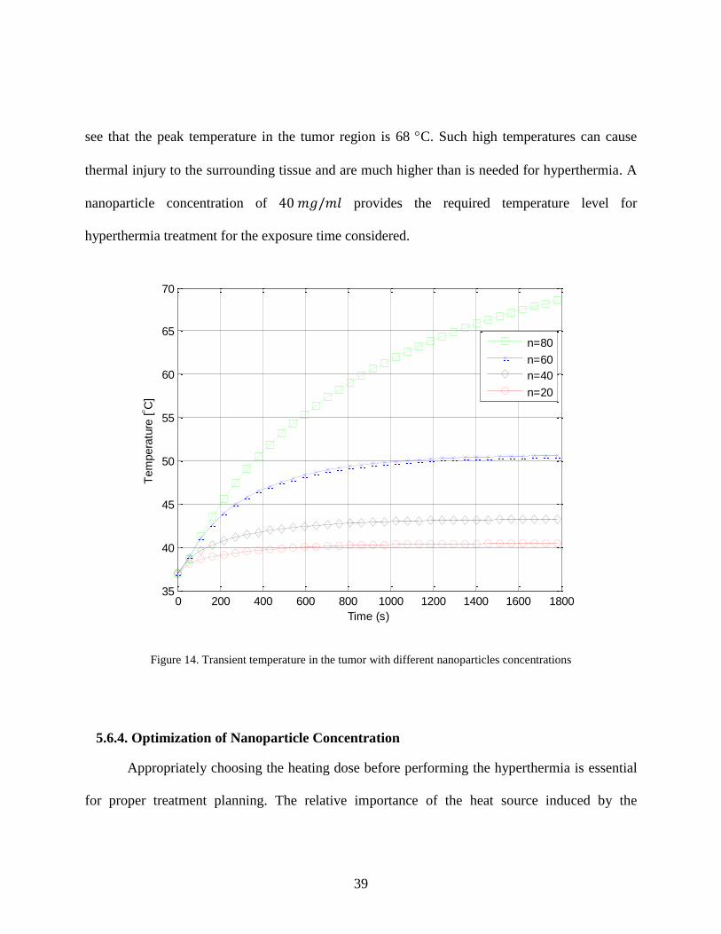
5.6.3. Effect of Nanoparticle Concentration on the Heating Behavior
Figure 14 shows the influence of the nanoparticle concentration on the increase in the
tumor temperature. With a magnetic nanoparticles with a concentration equals of 60 𝑚𝑔/𝑚𝑙, we
0 200 400 600 800 1000 1200 1400 1600 180037
38
39
40
41
42
43
44
Time (s)
Tem
pera
ture
[ C
]
"=15
"=35
"=55
"=65
39
see that the peak temperature in the tumor region is 68 C. Such high temperatures can cause
thermal injury to the surrounding tissue and are much higher than is needed for hyperthermia. A
nanoparticle concentration of 40 𝑚𝑔/𝑚𝑙 provides the required temperature level for
hyperthermia treatment for the exposure time considered.
Figure 14. Transient temperature in the tumor with different nanoparticles concentrations
5.6.4. Optimization of Nanoparticle Concentration
Appropriately choosing the heating dose before performing the hyperthermia is essential
for proper treatment planning. The relative importance of the heat source induced by the
0 200 400 600 800 1000 1200 1400 1600 180035
40
45
50
55
60
65
70
Time (s)
Tem
pera
ture
[ C
]
n=80
n=60
n=40
n=20
40
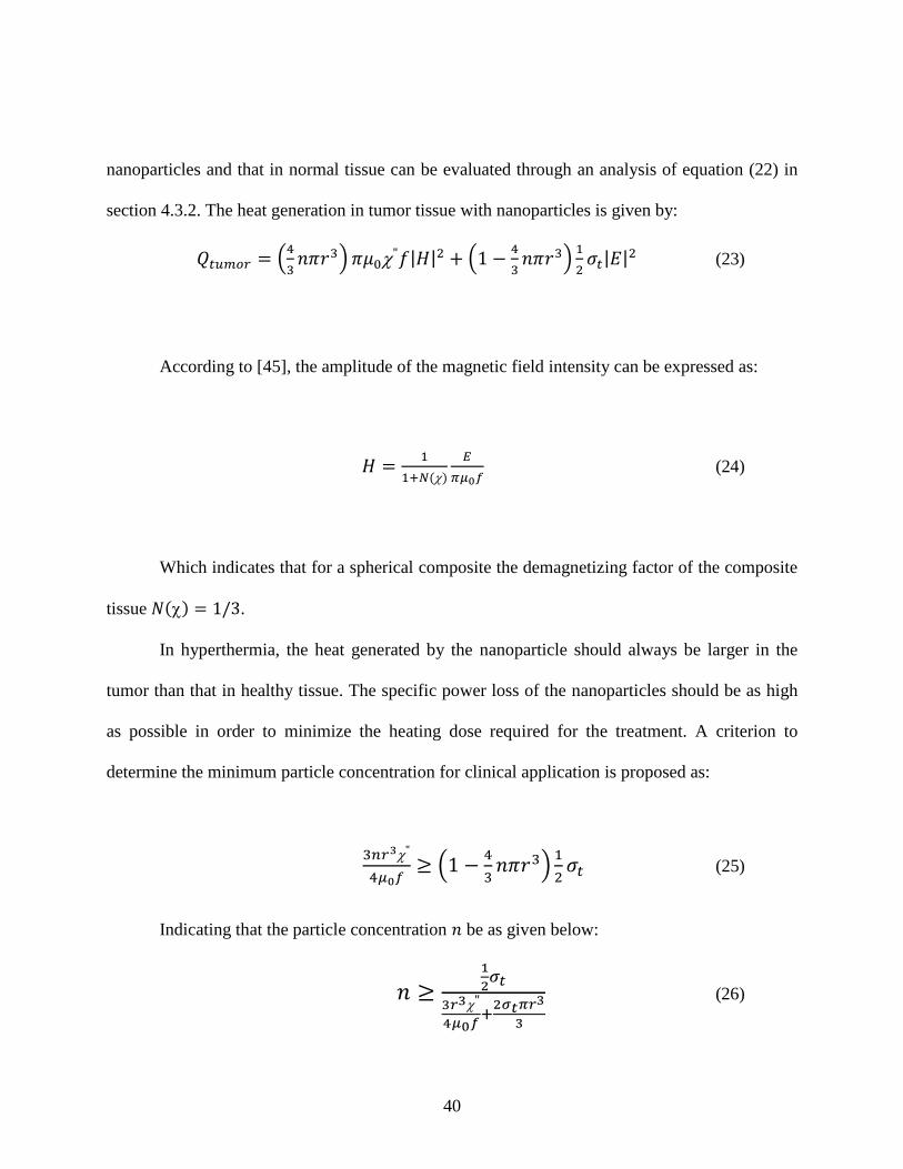
nanoparticles and that in normal tissue can be evaluated through an analysis of equation (22) in
section 4.3.2. The heat generation in tumor tissue with nanoparticles is given by:
𝑄𝑡𝑢𝑚𝑜𝑟 = (4
3𝑛𝜋𝑟3) 𝜋𝜇0
"𝑓|𝐻|2 + (1 −4
3𝑛𝜋𝑟3)
1
2𝜎𝑡|𝐸|2 (23)
According to [45], the amplitude of the magnetic field intensity can be expressed as:
𝐻 =1
1+𝑁()
𝐸
𝜋𝜇0𝑓 (24)
Which indicates that for a spherical composite the demagnetizing factor of the composite
tissue 𝑁() = 1/3.
In hyperthermia, the heat generated by the nanoparticle should always be larger in the
tumor than that in healthy tissue. The specific power loss of the nanoparticles should be as high
as possible in order to minimize the heating dose required for the treatment. A criterion to
determine the minimum particle concentration for clinical application is proposed as:
3𝑛𝑟3"
4𝜇0𝑓≥ (1 −
4
3𝑛𝜋𝑟3)
1
2𝜎𝑡 (25)
Indicating that the particle concentration 𝑛 be as given below:
𝑛 ≥1
2𝜎𝑡
3𝑟3"
4𝜇0𝑓+
2𝜎𝑡𝜋𝑟3
3
(26)
41
5.7. Experimental Results
5.7.1. Solid Phantom
In most instances, experiments cannot be done on human bodies and hence for medical
research, phantoms are used. A phantom is prepared so as to simulate actual biological tissues
and allows one to study interactions between applied electromagnetic fields and the human body.
Phantoms provide a stable, controllable environment for such studies. Phantoms can be prepared
to simulate the whole body or specific tissues or organs in the body. The ways to prepare these
phantoms are available in the literature.
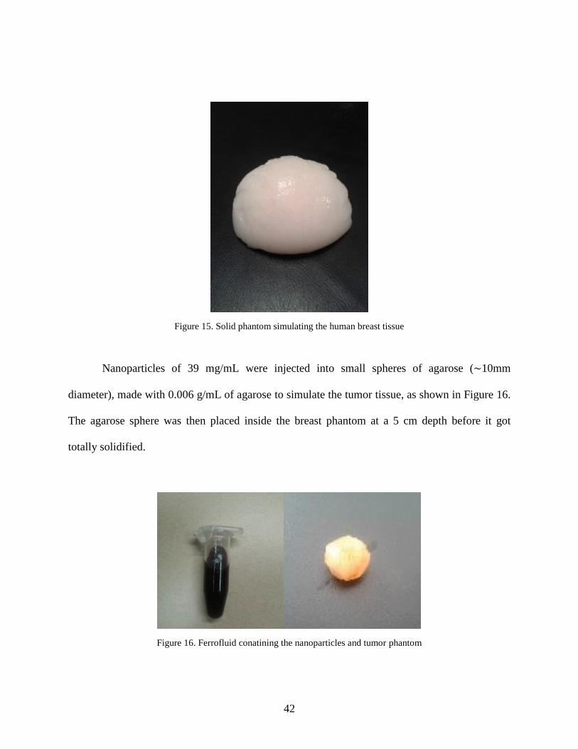
A human breast phantom using corn oil (150 ml), tri-distilled water (50 ml), neutral detergent
(30 ml), and agarose (4.5 g) [52] was made to simulate the relative permittivity and electrical
conductivity [12] of human breast fat tissue at 2.45 GHz. Figure 15 shows the phantom breast
tissue fabricated. The relative permittivity of breast fat is 5.28 and electrical conductivity is
0.105 S/m for 2.45 GHz. The dielectric constant of the breast phantom was measured using a
ring resonator [53] and was found to be 5.1 and 0.13 S/m, agreeing well with the reported
dielectric constants.
The tumor phantom was made using tri-distilled water (100 ml), ethanol (60 ml), and NaCl
(1g) mixed together and heated at ∼80◦C for 5 minutes. The measured permittivity for the
phantom mimicking the tumor was 59, which agrees well with the reported value of 60.
42
Figure 15. Solid phantom simulating the human breast tissue
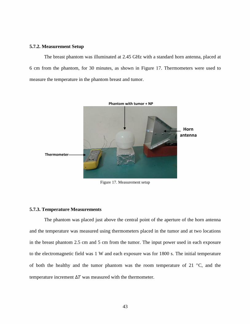
Nanoparticles of 39 mg/mL were injected into small spheres of agarose (∼10mm
diameter), made with 0.006 g/mL of agarose to simulate the tumor tissue, as shown in Figure 16.
The agarose sphere was then placed inside the breast phantom at a 5 cm depth before it got
totally solidified.
Figure 16. Ferrofluid conatining the nanoparticles and tumor phantom
43
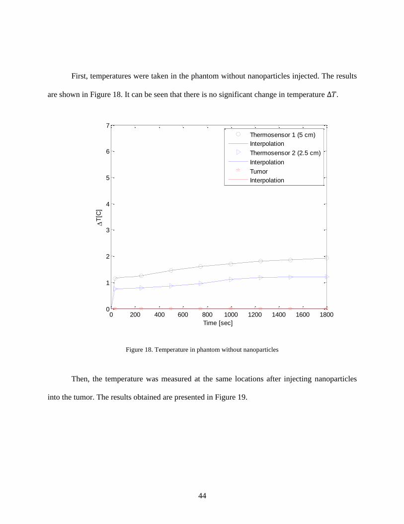
5.7.2. Measurement Setup
The breast phantom was illuminated at 2.45 GHz with a standard horn antenna, placed at
6 cm from the phantom, for 30 minutes, as shown in Figure 17. Thermometers were used to
measure the temperature in the phantom breast and tumor.
Figure 17. Measurement setup
5.7.3. Temperature Measurements
The phantom was placed just above the central point of the aperture of the horn antenna
and the temperature was measured using thermometers placed in the tumor and at two locations
in the breast phantom 2.5 cm and 5 cm from the tumor. The input power used in each exposure
to the electromagnetic field was 1 W and each exposure was for 1800 s. The initial temperature
of both the healthy and the tumor phantom was the room temperature of 21 C, and the
temperature increment ∆𝑇 was measured with the thermometer.
Thermometer
Phantom with tumor + NP
Horn antenna
44
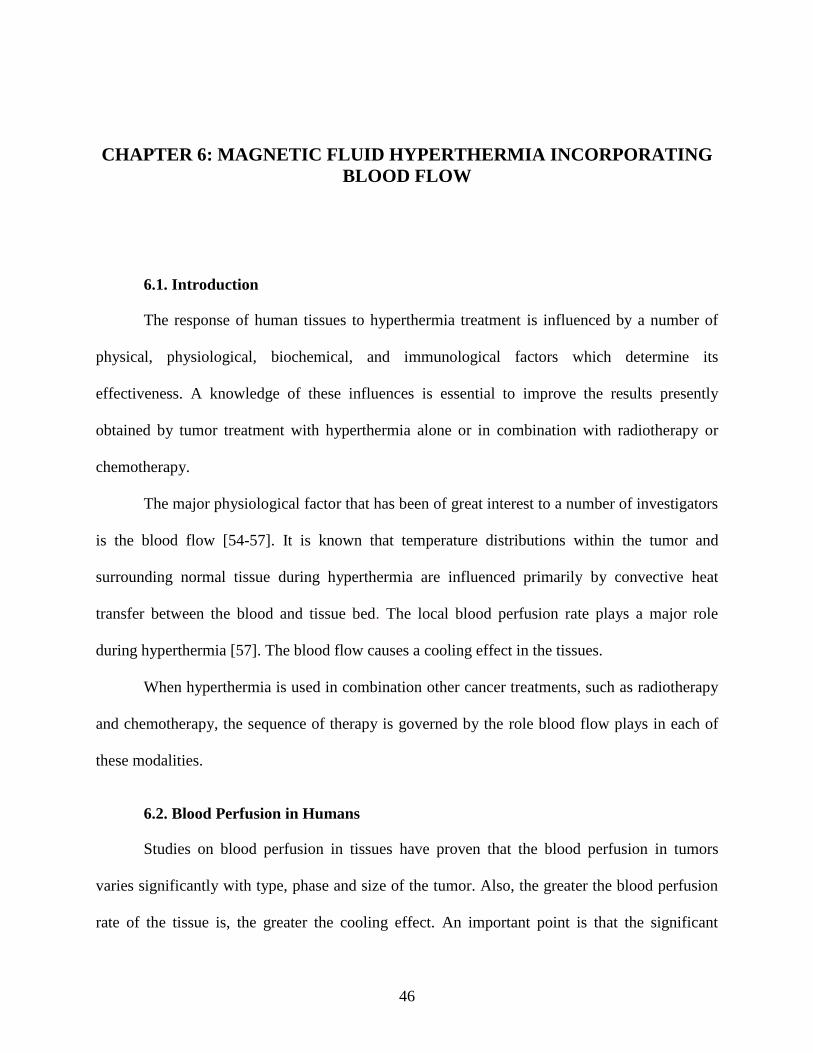
First, temperatures were taken in the phantom without nanoparticles injected. The results
are shown in Figure 18. It can be seen that there is no significant change in temperature ∆𝑇.
Figure 18. Temperature in phantom without nanoparticles
Then, the temperature was measured at the same locations after injecting nanoparticles
into the tumor. The results obtained are presented in Figure 19.
0 200 400 600 800 1000 1200 1400 1600 18000
1
2
3
4
5
6
7
Time [sec]
T
[C]
Thermosensor 1 (5 cm)
Interpolation
Thermosensor 2 (2.5 cm)
Interpolation
Tumor
Interpolation

45
Figure 19. Temperature in phantom with nanoparticles
The measurements validate the results obtained with the simulations. There is an increase
in the tumor around 6 - 7C, which indicates that the nanoparticles exhibit a highly focused
heating in the tumor tissue region, which is much higher than that in the surrounding healthy
tissue.
0 200 400 600 800 1000 1200 1400 1600 18000
1
2
3
4
5
6
7
Time [sec]
T
[C]
Thermosensor 1 (5 cm)
Interpolation
Thermosensor 2 (2.5 cm)
Interpolation
Tumor
Interpolation
46
CHAPTER 6: MAGNETIC FLUID HYPERTHERMIA INCORPORATING
BLOOD FLOW
6.1. Introduction
The response of human tissues to hyperthermia treatment is influenced by a number of
physical, physiological, biochemical, and immunological factors which determine its
effectiveness. A knowledge of these influences is essential to improve the results presently
obtained by tumor treatment with hyperthermia alone or in combination with radiotherapy or
chemotherapy.
The major physiological factor that has been of great interest to a number of investigators
is the blood flow [54-57]. It is known that temperature distributions within the tumor and
surrounding normal tissue during hyperthermia are influenced primarily by convective heat
transfer between the blood and tissue bed. The local blood perfusion rate plays a major role
during hyperthermia [57]. The blood flow causes a cooling effect in the tissues.
When hyperthermia is used in combination other cancer treatments, such as radiotherapy
and chemotherapy, the sequence of therapy is governed by the role blood flow plays in each of
these modalities.
6.2. Blood Perfusion in Humans
Studies on blood perfusion in tissues have proven that the blood perfusion in tumors
varies significantly with type, phase and size of the tumor. Also, the greater the blood perfusion
rate of the tissue is, the greater the cooling effect. An important point is that the significant
47
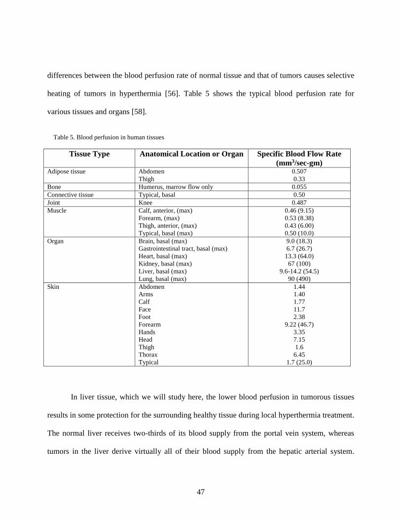
differences between the blood perfusion rate of normal tissue and that of tumors causes selective
heating of tumors in hyperthermia [56]. Table 5 shows the typical blood perfusion rate for
various tissues and organs [58].
Table 5. Blood perfusion in human tissues
Tissue Type Anatomical Location or Organ Specific Blood Flow Rate
(mm3/sec-gm) Adipose tissue Abdomen
Thigh
0.507
0.33
Bone Humerus, marrow flow only 0.055
Connective tissue Typical, basal 0.50
Joint Knee 0.487
Muscle Calf, anterior, (max)
Forearm, (max)
Thigh, anterior, (max)
Typical, basal (max)
0.46 (9.15)
0.53 (8.38)
0.43 (6.00)
0.50 (10.0)
Organ Brain, basal (max)
Gastrointestinal tract, basal (max)
Heart, basal (max)
Kidney, basal (max)
Liver, basal (max)
Lung, basal (max)
9.0 (18.3)
6.7 (26.7)
13.3 (64.0)
67 (100)
9.6-14.2 (54.5)
90 (490)
Skin Abdomen
Arms
Calf
Face
Foot
Forearm
Hands
Head
Thigh
Thorax
Typical
1.44
1.40
1.77
11.7
2.38
9.22 (46.7)
3.35
7.15
1.6
6.45
1.7 (25.0)
In liver tissue, which we will study here, the lower blood perfusion in tumorous tissues
results in some protection for the surrounding healthy tissue during local hyperthermia treatment.
The normal liver receives two-thirds of its blood supply from the portal vein system, whereas
tumors in the liver derive virtually all of their blood supply from the hepatic arterial system.
48
Thus, for hepatic tumors, substances injected into the hepatic arterial system will be
preferentially delivered to the liver tumor [59]. Hence, the use of magnetic nanoparticles by
injecting them into the tumor via arterial embolization, provides an effective way to kill tumor
cells.
In arterial embolization, also known as trans-arterial embolization (or TAE), a catheter (a
thin, flexible tube) is inserted into an artery through a small cut in the inner thigh and threaded
up into the hepatic artery in the liver. A dye is injected into the bloodstream so that the doctor
monitor the path of the catheter via angiography. The nanoparticles can then be injected through
the catheter.
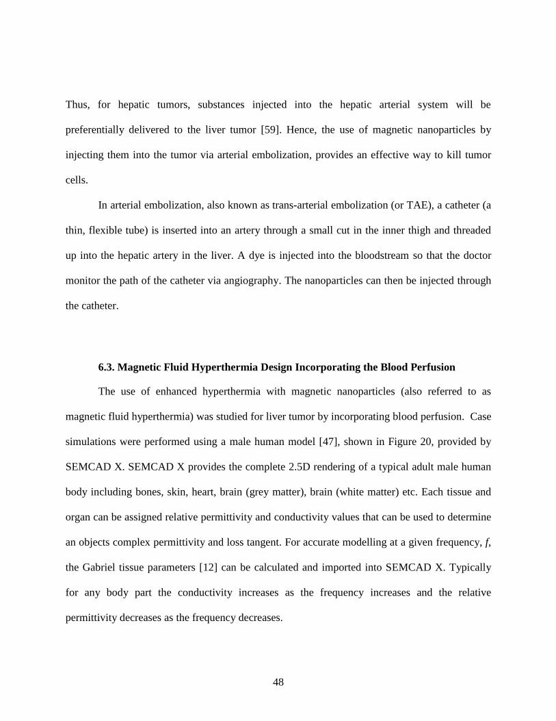
6.3. Magnetic Fluid Hyperthermia Design Incorporating the Blood Perfusion
The use of enhanced hyperthermia with magnetic nanoparticles (also referred to as
magnetic fluid hyperthermia) was studied for liver tumor by incorporating blood perfusion. Case
simulations were performed using a male human model [47], shown in Figure 20, provided by
SEMCAD X. SEMCAD X provides the complete 2.5D rendering of a typical adult male human
body including bones, skin, heart, brain (grey matter), brain (white matter) etc. Each tissue and
organ can be assigned relative permittivity and conductivity values that can be used to determine
an objects complex permittivity and loss tangent. For accurate modelling at a given frequency, f,
the Gabriel tissue parameters [12] can be calculated and imported into SEMCAD X. Typically
for any body part the conductivity increases as the frequency increases and the relative
permittivity decreases as the frequency decreases.
49
Figure 20. Human model in SEMCAD X
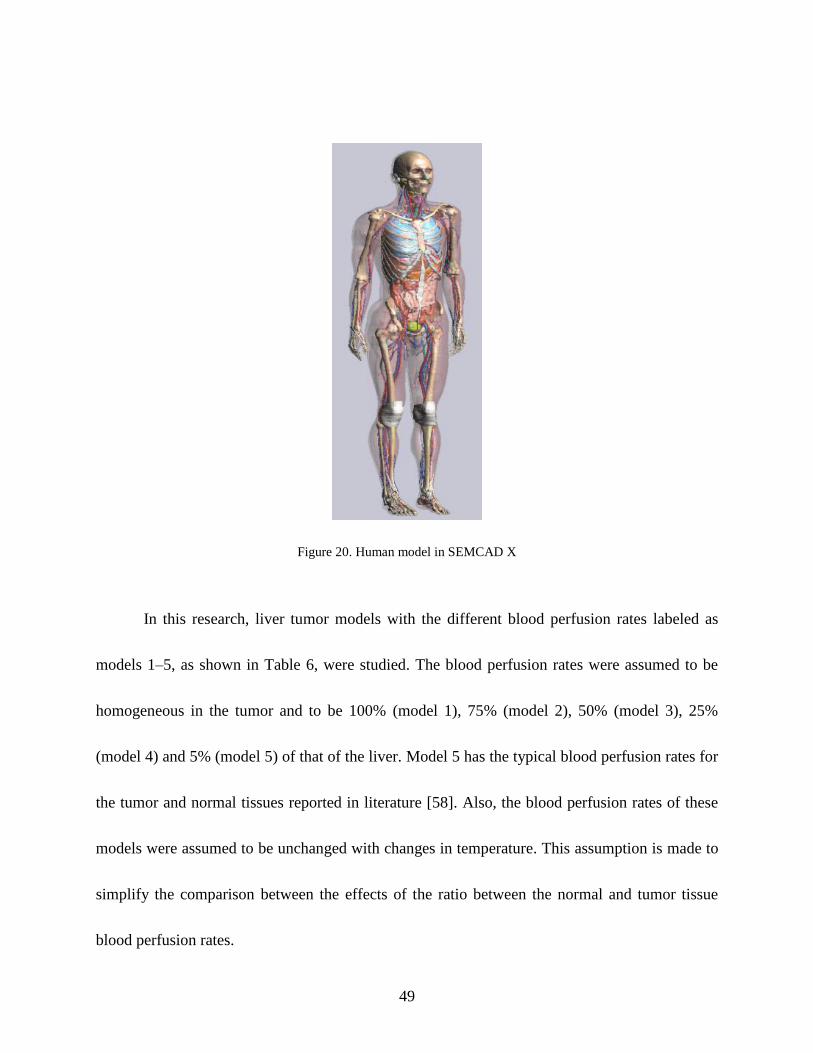
In this research, liver tumor models with the different blood perfusion rates labeled as
models 1–5, as shown in Table 6, were studied. The blood perfusion rates were assumed to be
homogeneous in the tumor and to be 100% (model 1), 75% (model 2), 50% (model 3), 25%
(model 4) and 5% (model 5) of that of the liver. Model 5 has the typical blood perfusion rates for
the tumor and normal tissues reported in literature [58]. Also, the blood perfusion rates of these
models were assumed to be unchanged with changes in temperature. This assumption is made to
simplify the comparison between the effects of the ratio between the normal and tumor tissue
blood perfusion rates.
50
Table 6. Models with different blood perfusion rates
Model Tumor Blood Perfusion
(ml/min/kg)
Liver Blood Perfusion
(ml/min/kg)
1 600 600
2 450 600
3 300 600
4 150 600
5 30 600
For this study, the liver and tumor are illuminated at 2.45 GHz with a standard horn
antenna placed close to the surface of the body. A 1 cm tumor size is located inside the left lobe
of the liver at approximately 50 mm from the surface. A ferrofluid containing iron oxide
nanoparticles of concentration 40 mg/mL was injected into the tumor.
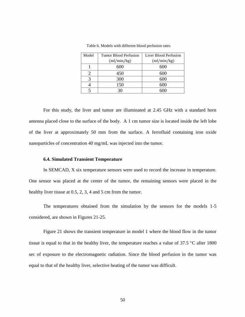
6.4. Simulated Transient Temperature
In SEMCAD, X six temperature sensors were used to record the increase in temperature.
One sensor was placed at the center of the tumor, the remaining sensors were placed in the
healthy liver tissue at 0.5, 2, 3, 4 and 5 cm from the tumor.
The temperatures obtained from the simulation by the sensors for the models 1-5
considered, are shown in Figures 21-25.
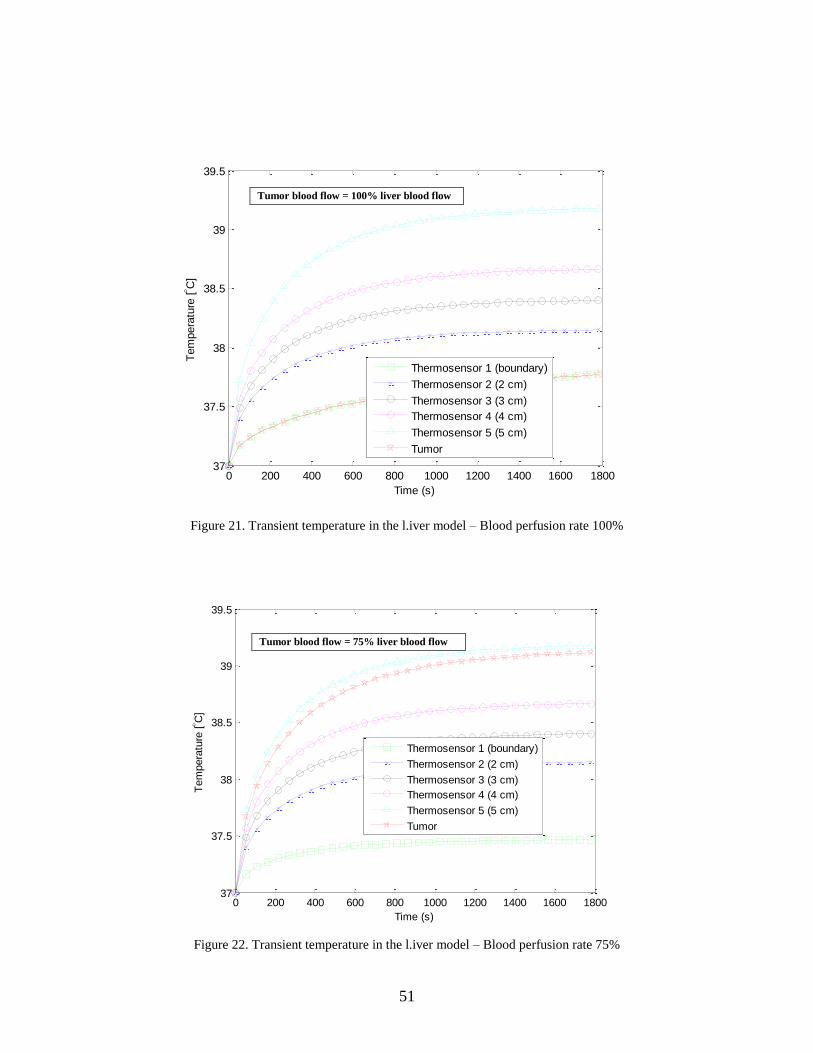
Figure 21 shows the transient temperature in model 1 where the blood flow in the tumor
tissue is equal to that in the healthy liver, the temperature reaches a value of 37.5 C after 1800
sec of exposure to the electromagnetic radiation. Since the blood perfusion in the tumor was
equal to that of the healthy liver, selective heating of the tumor was difficult.
51
Figure 21. Transient temperature in the l.iver model – Blood perfusion rate 100%
Figure 22. Transient temperature in the l.iver model – Blood perfusion rate 75%
0 200 400 600 800 1000 1200 1400 1600 180037
37.5
38
38.5
39
39.5
Time (s)
Tem
pera
ture
[ C
]
Thermosensor 1 (boundary)
Thermosensor 2 (2 cm)
Thermosensor 3 (3 cm)
Thermosensor 4 (4 cm)
Thermosensor 5 (5 cm)
Tumor
0 200 400 600 800 1000 1200 1400 1600 180037
37.5
38
38.5
39
39.5
Time (s)
Tem
pera
ture
[ C
]
Thermosensor 1 (boundary)
Thermosensor 2 (2 cm)
Thermosensor 3 (3 cm)
Thermosensor 4 (4 cm)
Thermosensor 5 (5 cm)
Tumor
Tumor blood flow = 100% liver blood flow
Tumor blood flow = 75% liver blood flow
52
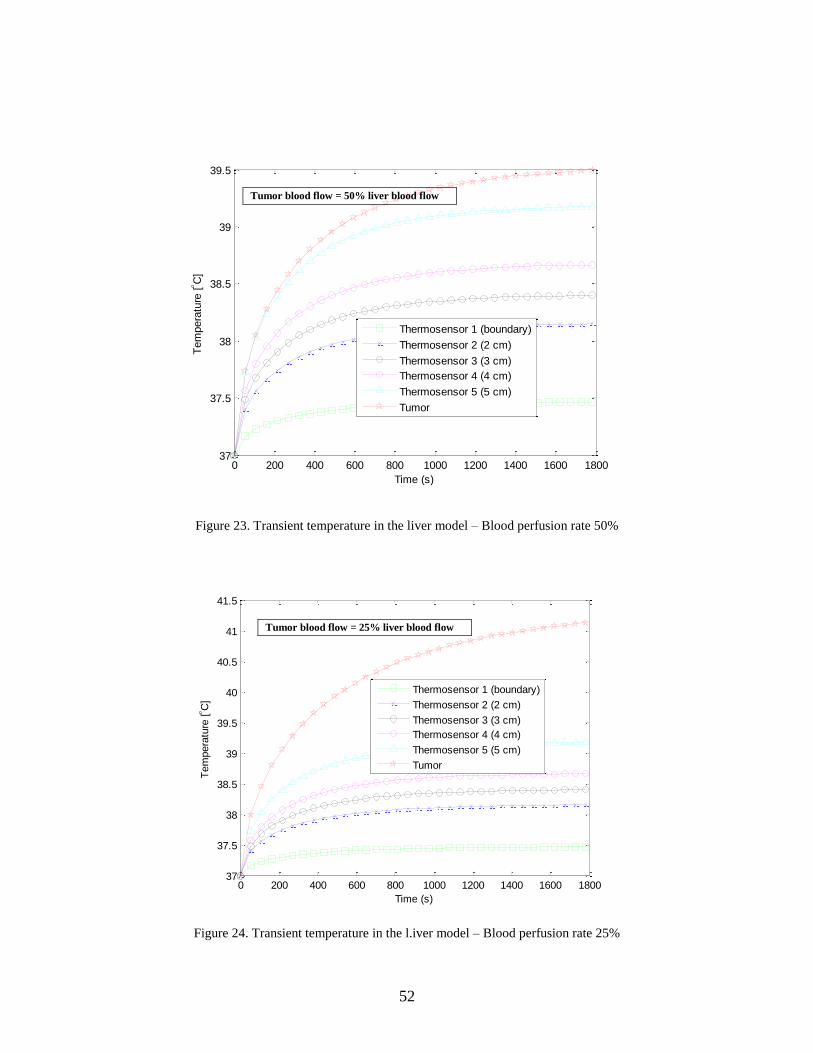
Figure 23. Transient temperature in the liver model – Blood perfusion rate 50%
Figure 24. Transient temperature in the l.iver model – Blood perfusion rate 25%
0 200 400 600 800 1000 1200 1400 1600 180037
37.5
38
38.5
39
39.5
Time (s)
Tem
pera
ture
[ C
]
Thermosensor 1 (boundary)
Thermosensor 2 (2 cm)
Thermosensor 3 (3 cm)
Thermosensor 4 (4 cm)
Thermosensor 5 (5 cm)
Tumor
0 200 400 600 800 1000 1200 1400 1600 180037
37.5
38
38.5
39
39.5
40
40.5
41
41.5
Time (s)
Tem
pera
ture
[ C
]
Thermosensor 1 (boundary)
Thermosensor 2 (2 cm)
Thermosensor 3 (3 cm)
Thermosensor 4 (4 cm)
Thermosensor 5 (5 cm)
Tumor
Tumor blood flow = 50% liver blood flow
Tumor blood flow = 25% liver blood flow
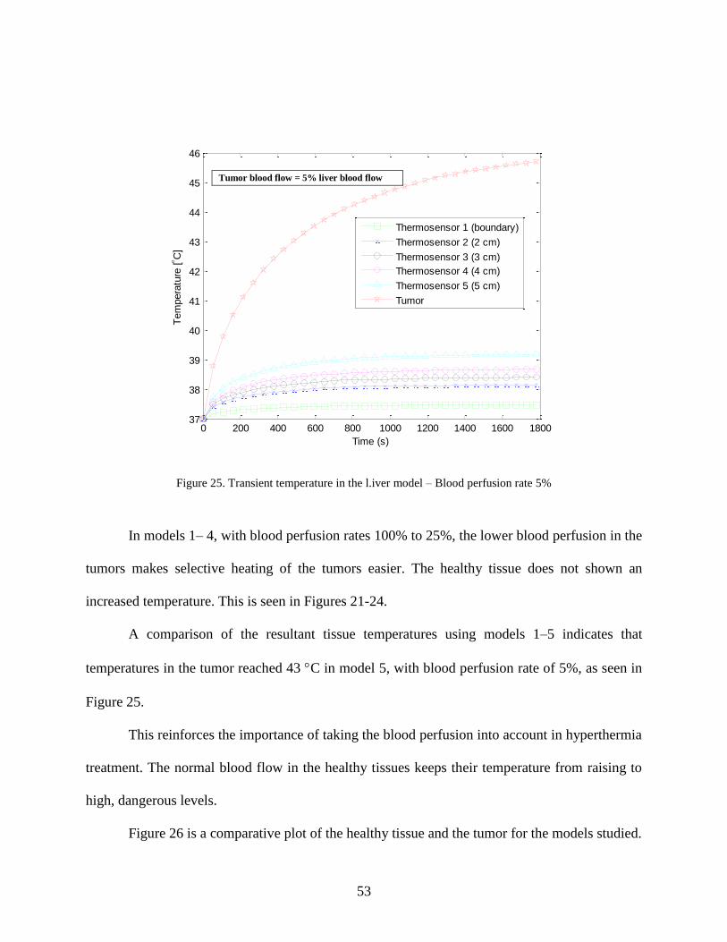
53
Figure 25. Transient temperature in the l.iver model – Blood perfusion rate 5%
In models 1– 4, with blood perfusion rates 100% to 25%, the lower blood perfusion in the
tumors makes selective heating of the tumors easier. The healthy tissue does not shown an
increased temperature. This is seen in Figures 21-24.
A comparison of the resultant tissue temperatures using models 1–5 indicates that
temperatures in the tumor reached 43 C in model 5, with blood perfusion rate of 5%, as seen in
Figure 25.
This reinforces the importance of taking the blood perfusion into account in hyperthermia
treatment. The normal blood flow in the healthy tissues keeps their temperature from raising to
high, dangerous levels.
Figure 26 is a comparative plot of the healthy tissue and the tumor for the models studied.
0 200 400 600 800 1000 1200 1400 1600 180037
38
39
40
41
42
43
44
45
46
Time (s)
Tem
pera
ture
[ C
]
Thermosensor 1 (boundary)
Thermosensor 2 (2 cm)
Thermosensor 3 (3 cm)
Thermosensor 4 (4 cm)
Thermosensor 5 (5 cm)
Tumor
Tumor blood flow = 5% liver blood flow
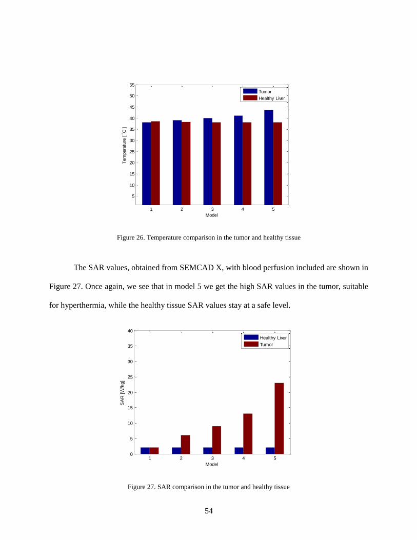
54
Figure 26. Temperature comparison in the tumor and healthy tissue
The SAR values, obtained from SEMCAD X, with blood perfusion included are shown in
Figure 27. Once again, we see that in model 5 we get the high SAR values in the tumor, suitable
for hyperthermia, while the healthy tissue SAR values stay at a safe level.
Figure 27. SAR comparison in the tumor and healthy tissue
1 2 3 4 5
5
10
15
20
25
30
35
40
45
50
55
Model
Tem
pera
ture
[ C
]
Tumor
Healthy Liver
1 2 3 4 50
5
10
15
20
25
30
35
40
Model
SA
R [
W/k
g]
Healthy Liver
Tumor

55
Since the nanoparticle characteristics play a major role in the heating and the SAR for
hyperthermia, a study of the effect of the nanoparticle concentration was done while including
the blood perfusion. The particle radius was kept at 18 mm and the concentration were varied
from 40 mg/mL to 60 mg/mL for each of the five models.
The results for the temperature in the tumor are shown in Figure 28. For model 5, with
the lowest blood perfusion, a concentration of 40 mg/mL gives the desired temperature for
hyperthermia.
Figure 28. Temperature increase in the tumor as a function of nanoparticle concentration
0 10 20 30 40 50 60 70 800
10
20
30
40
50
60
70
80
Concentration [mg/mL]
Tem
pera
ture
[oC
]
Model 1
Model 2
Model 3
Model 4
Model 5

56
6.5. Experimental Results using a Simplified Phantom
A simplified phantom model was made to carry out an experimental demonstration of the
blood flow cooling effect in magnetic fluid hyperthermia. Figure 29 shows a cylindrical solid
phantom liver size L= 6 cm and r = 8.5 cm. In this research, only the hepatic portal vein is
considered. The hepatic portal vein is modelled as a cylindrical hole of 20 mm in diameter within
the phantom. Saline solution poured through the liver phantom was used to simulate the cooling
effect due to blood flow in the vein. The velocity of the saline solution is controlled by changing
the diameter of a small hole in a rubber sheet placed at the bottom of the phantom.
The relative permittivity of this phantom is 47 and the conductivity is 2.2 S/m, which is
equivalent to the electrical constants of human liver at 2.45 GHz. A 0.35 % saline solution is
poured into the cylindrical hole modeling the hepatic portal vein. The value of the conductivity
of the 0.35 % saline solution is 2.1 S/m, which is almost the same value that the human blood at
2.45 GHz. During the experiment, the saline solution is poured continuously. The permittivity of
the tumor phantom was 59 and it was injected with iron oxide nanoparticle concentration of 40
mg/ml and placed at 50 mm from the surface.
Figure 29. Simplified liver model
Saline Solution
Tumor
𝑟 = 8.5 cm
𝐿 = 6 cm
Rubber sheet
Liver phantom
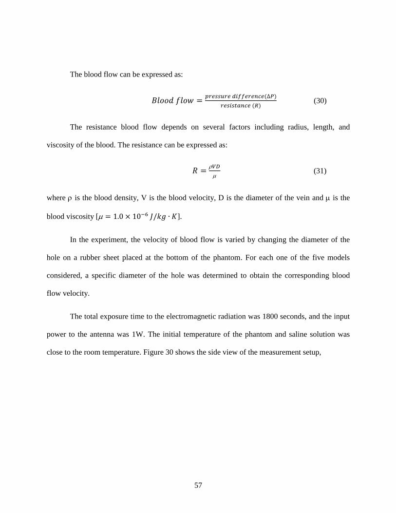
57
The blood flow can be expressed as:
𝐵𝑙𝑜𝑜𝑑 𝑓𝑙𝑜𝑤 =𝑝𝑟𝑒𝑠𝑠𝑢𝑟𝑒 𝑑𝑖𝑓𝑓𝑒𝑟𝑒𝑛𝑐𝑒(∆𝑃)
𝑟𝑒𝑠𝑖𝑠𝑡𝑎𝑛𝑐𝑒 (𝑅) (30)
The resistance blood flow depends on several factors including radius, length, and
viscosity of the blood. The resistance can be expressed as:
𝑅 =𝑉𝐷
(31)
where is the blood density, V is the blood velocity, D is the diameter of the vein and is the
blood viscosity [ = 1.0 × 10⁻⁶ 𝐽/𝑘𝑔 ∙ 𝐾].
In the experiment, the velocity of blood flow is varied by changing the diameter of the
hole on a rubber sheet placed at the bottom of the phantom. For each one of the five models
considered, a specific diameter of the hole was determined to obtain the corresponding blood
flow velocity.
The total exposure time to the electromagnetic radiation was 1800 seconds, and the input
power to the antenna was 1W. The initial temperature of the phantom and saline solution was
close to the room temperature. Figure 30 shows the side view of the measurement setup,

58
Figure 30. Liver phantom measurement setup – Side view
and Figure 31 is a top view of the liver phantom model showing the cylindrical holes to pour
saline solution into.
Figure 31. Liver phantom model – Top view
Thermometer
Liver phantom with tumor + NP
Rubber sheet
Horn antenna
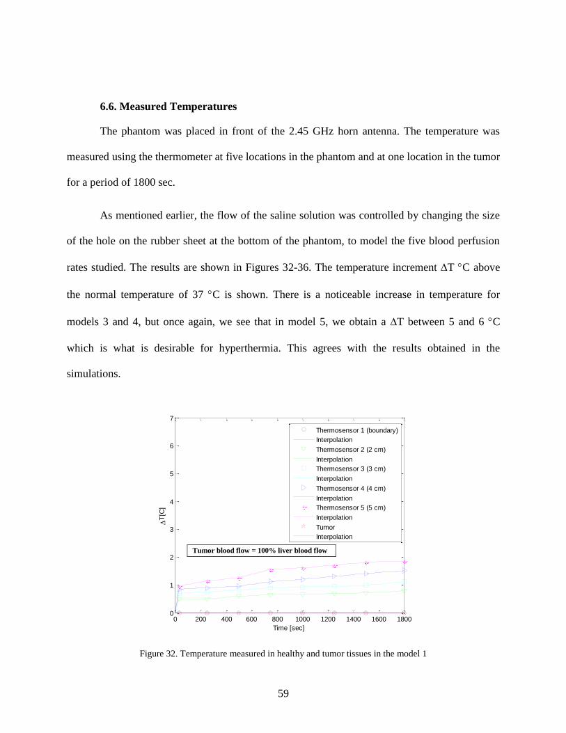
59
6.6. Measured Temperatures
The phantom was placed in front of the 2.45 GHz horn antenna. The temperature was
measured using the thermometer at five locations in the phantom and at one location in the tumor
for a period of 1800 sec.
As mentioned earlier, the flow of the saline solution was controlled by changing the size
of the hole on the rubber sheet at the bottom of the phantom, to model the five blood perfusion
rates studied. The results are shown in Figures 32-36. The temperature increment T C above
the normal temperature of 37 C is shown. There is a noticeable increase in temperature for
models 3 and 4, but once again, we see that in model 5, we obtain a T between 5 and 6 C
which is what is desirable for hyperthermia. This agrees with the results obtained in the
simulations.
Figure 32. Temperature measured in healthy and tumor tissues in the model 1
0 200 400 600 800 1000 1200 1400 1600 18000
1
2
3
4
5
6
7
Time [sec]
T
[C]
Thermosensor 1 (boundary)
Interpolation
Thermosensor 2 (2 cm)
Interpolation
Thermosensor 3 (3 cm)
Interpolation
Thermosensor 4 (4 cm)
Interpolation
Thermosensor 5 (5 cm)
Interpolation
Tumor
Interpolation
Tumor blood flow = 100% liver blood flow
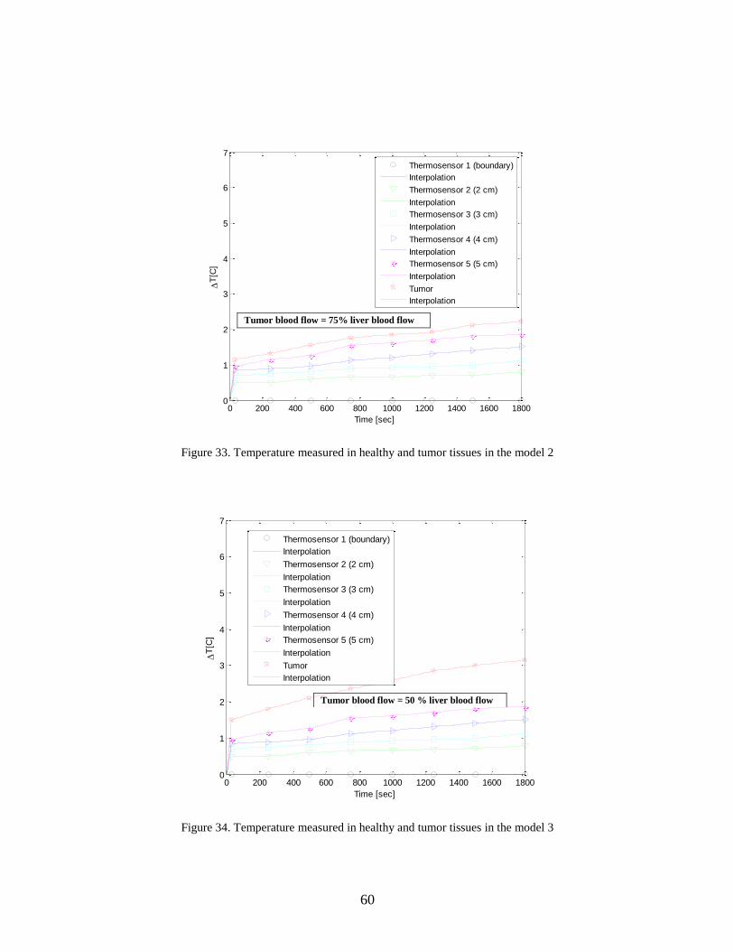
60
Figure 33. Temperature measured in healthy and tumor tissues in the model 2
Figure 34. Temperature measured in healthy and tumor tissues in the model 3
0 200 400 600 800 1000 1200 1400 1600 18000
1
2
3
4
5
6
7
Time [sec]
T
[C]
Thermosensor 1 (boundary)
Interpolation
Thermosensor 2 (2 cm)
Interpolation
Thermosensor 3 (3 cm)
Interpolation
Thermosensor 4 (4 cm)
Interpolation
Thermosensor 5 (5 cm)
Interpolation
Tumor
Interpolation
0 200 400 600 800 1000 1200 1400 1600 18000
1
2
3
4
5
6
7
Time [sec]
T
[C]
Thermosensor 1 (boundary)
Interpolation
Thermosensor 2 (2 cm)
Interpolation
Thermosensor 3 (3 cm)
Interpolation
Thermosensor 4 (4 cm)
Interpolation
Thermosensor 5 (5 cm)
Interpolation
Tumor
Interpolation
Tumor blood flow = 75% liver blood flow
Tumor blood flow = 50 % liver blood flow
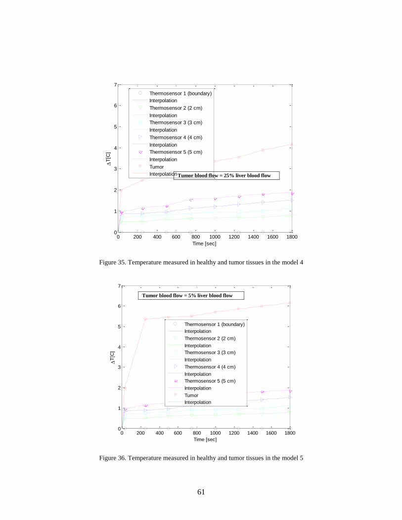
61
Figure 35. Temperature measured in healthy and tumor tissues in the model 4
Figure 36. Temperature measured in healthy and tumor tissues in the model 5
0 200 400 600 800 1000 1200 1400 1600 18000
1
2
3
4
5
6
7
Time [sec]
T
[C]
Thermosensor 1 (boundary)
Interpolation
Thermosensor 2 (2 cm)
Interpolation
Thermosensor 3 (3 cm)
Interpolation
Thermosensor 4 (4 cm)
Interpolation
Thermosensor 5 (5 cm)
Interpolation
Tumor
Interpolation
0 200 400 600 800 1000 1200 1400 1600 18000
1
2
3
4
5
6
7
Time [sec]
T
[C]
Thermosensor 1 (boundary)
Interpolation
Thermosensor 2 (2 cm)
Interpolation
Thermosensor 3 (3 cm)
Interpolation
Thermosensor 4 (4 cm)
Interpolation
Thermosensor 5 (5 cm)
Interpolation
Tumor
Interpolation
Tumor blood flow = 25% liver blood flow
Tumor blood flow = 5% liver blood flow

62
6.7. Use of Magnetic Fluid Hyperthermia in Human Tissues
Although magnetic fluid hyperthermia is an effective cancer therapy, there are limitations
that restrict its use to tumors growing in specific tissues in the body. These limitations include
blood perfusion, which leads to large amount of blood removing heat from the tissue and the size
the nanoparticles, which may restrict them from traveling into the smaller capillaries inside the
tumor. Such restrictions prevent magnetic fluid hyperthermia from treating brain tumors where
the blood-brain barrier does not allow effective injection of nanoparticles into the tumor. In lung
tissues, the high blood perfusion results in rapid heat dissipation even before the nanoparticles
can even reach the desired increased temperature needed to kill the cancerous cells. The low heat
diffusivity and difficulty in pinpointing tumor locations in bone cancer also makes magnetic
fluid hyperthermia a less effective treatment approach.

63
CHAPTER 7: CONCLUSIONS
The technical challenge in hyperthermia treatment is to heat the tumor to the appropriate
therapeutic temperature without causing damage to the surrounding healthy tissue. The results
presented in this research show that conventional hyperthermia treatment can be enhanced
through the use of magnetic nanoparticles.
A system with a microwave applicator at 2.45 GHz, magnetic nanoparticles and
temperature monitoring sensors was modeled to effectively study hyperthermia treatment for
cancerous tissues in the breast and in the liver.
Simulated results for enhanced hyperthermia breast cancer were obtained using HFSS
and SEMCAD X and values for the SAR and transient temperature in the healthy tissue and the
tumor were presented. Using Penne’s bioheat transfer equation and comparing results with and
without iron oxide nanoparticles injected in the tumor, it was seen that the presence of
nanoparticles allowed for the required increase in temperature in a short period of time. Various
characteristics of the nanoparticles such as size, concentration, and susceptibility were
considered. It was seen that a radius of 18 nm and a concentration of 40 mg/mL provided the
most desirable results. Temperatures in the tumor reached that required to kill the cancer cells
while the healthy tissue remained at a safe temperatures.
Experiments were conducted on a phantom model and the results validated those
obtained through simulations.
64
As the blood flow in the body plays an important role in maintaining the body
temperature, the effect of blood perfusion in magnetic fluid hyperthermia was also studied. Here,
a tumor in the liver was injected with nanoparticles and five different blood perfusion rates were
studied. Using a human male model, available in SEMCAD X, and appropriate values for the
dielectric constant and conductivities in the tissue, the incremental increase in the temperature
was obtained in the liver and in the tumor. When the blood perfusion rate in the tumor was low,
as in the case found in liver tumors, the rise in temperature was higher in the tumor than in the
healthy tissue.
Experiments were done using a liver phantom model and allowing 0.35% saline solution
flow through it to simulate blood flow. The results obtained agree with those of the SEMCAD X
simulation.
It was shown that the use of magnetic nanoparticles does provide a more effective
hyperthermia treatment for cancerous tumors in the breast and liver.
65
REFERENCES
[1] I.M Zaryabova and M. Ivanova , "Electromagnetic field occupational exposure: non-thermal
vs. thermal effects," Electromagn. Biol Med., vol. 32, pp. 145-154, Jun. 2013.
[2] C. Johnson A. Guy, "Nonionizing Electromagnetic Wave Effects in Biological Materials and
systems," IEEE Biolog. Effe. of Electrom. Radiation, pp. 47-73, 1983.
[3] A. Vorst et al., RF Microwave Interaction with Biological Tissues. Wiley Series in
Microwave and Optical Engineering, Honoken NJ, 2006.
[4] H. P Schawn and G. Morri, "The Absorption of Electromagnetic Energy in Body Tissues,"
IEEE Biolog. Effe. of Electrom. Radiation, pp. 6-21, 1983.
[5] J.W. Hand and G. Ter Haar, "Heating techniques in hyperthermia," Br. J. Radiol., vol.54, pp.
443-466, 1981.
[6] I. Green, "Hyperthermia alone or combined with chemotherapy for treatment of cancer,"
AHCPR Health Technology Reports, vol. 2, pp.1-16, 1991.
[7] P. Wust et al., "Hyperthermia in combined treatment of cancer," Lancet Oncol., vol. 3, pp.
487-497, 2002.
[8] E.R Lee, "Electromagnetic superficial heating technology," Thermoradiotherapy and
thermochemotherapy, Springer-Verlag, pp.193-217, 1995.
[9] S. Wust et al., "Electromagnetic deep heating technology," Thermoradiotherapy and
thermochemotherapy, Springer-Verlag, pp.219-251, 1995.
[10] R. Antolini et al., "Absorbed power distributions from single or multiple waveguide
applicators during microwaved hyperthermia," Phys. Med. Biol., vol. 31, pp. 1005-1019, 1986.
66
[11] K.S Cole and R.H Cole, "Dispersion and absorption in dielectrics I. Alternating current
characteristics," The J. of Chemical Physics, vol. 9, pp. 341-351, 1941.
[12] C. Gabriel, "Compilation of the Dielectric Properties of Body Tissues at RF and Microwave
Frequencies," King's College, London, Department of Physics, 1996.
[13] E.C Van E.Cet al., "Regional hyperthermia of pelvic tumours using the Utrecgt Coaxial
TEM system: a feasibility study," Int. J. Hyperthermia, vol. 11, pp.173-186, 1995.
[14] Y. Kotsuka et al., "Development of inductive regional heating system for breast
hyperthermia," IEEE Trans. Microw. Theory Tech., vol. 48, 1807-1814, 2000.
[15] B.Mortimer and S. L. Osborne, “Tissue heating by short wave diathermy,” The Journal of
the American Medical Association, vol. 103, pp. 1413–1418, 1935.
[16] W. T. Szymanowski and R. A. Hicks, “Further studies of biologic action of ultra-high
frequency currents,”The Journal of Infectious Diseases, vol. 50, p. 471, 1932.
[17] R.K Gilchrist et al, "Selective Inductive Heating of Lymph," Ann. of Surgery, vol. 146, pp.
596-606, 1957.
[18] W. W. Shingleton, “Selective heating and cooling of tissue in cancer chemotherapy,”
Annals of Surgery, vol. 156, pp. 408–416, 1962.
[19] M. von Ardenne and P. G. Reitnauer, “On the effect of hyperthermia on Ehrlich mouse
ascites cancer cells,” Archiv f¨ur Geschwulstforschung, vol. 26, no. 3, pp. 184–185, 1965.
[20] M. von Ardenne, “Principles and 1977 concept of cancer multistep therapy. Physiological
fundamentals of the new timing. Selectotherm local hyperthermy,” Archiv f¨ur
Geschwulstforschung, vol. 48, no. 6, pp. 504–520, 1978.

67
[21] M. von Ardenne and W. Kr‥uger, “Combined whole-body and local hyperthermia for
cancer treatment: CMT selectotherm technique,” Progress in Clinical and Biological Research,
vol. 107, pp. 705–713, 1982.
[22] H. S. Reinhold, J. van der Zee, N. S. Faithfull, G. van Rhoon, and J. Wike-Hooley, “Use of
the Pomp-Siemens hyperthermia cabin,” National Cancer Institute Monograph, vol. 61, pp.
371– 375, 1982.
[23] F.K. Storm et al., "Clinical RF hyperthermia by magnetic-loop induction: a new approach to
human cancer therapy," IEEE Trans. Microw. Theory Tech., vol. 30, pp. 1124-1158, 1982.
[24] M. A. Astrahan et al., “Heating characteristics of a helical microwave applicator for
transurethral hyperthermia of benign prostatic hyperplasia,” Int. J. Hyperthermia 7, 141–155,
1991.
[25] C. Moran et al., "Size-dependent joule heating of gold nanoparticles using capacitively
coupled radiofrequency fields," Nano. Research, vol.2, pp. 400-405, May 2009.
[26] R. Ben-Yosef, D. S. Kapp, “Direct clinical comparison of ultrasound and radiative
electromagnetic hyperthermia applicators in the same tumours,” International Journal of
Hyperthermia , 11, 1-10, 1995.
[27] P. F. Turner, A. Tumeh, and T. Schaefermeyer, “BSD-2000 approach for deep local and
regional hyperthermia: physics and technology,” Strahlentherapie und Onkologie, vol. 165, no.
10, pp. 738–741, 1989.

68
[28] P. F.Turner and T. Schaefermeyer, “BSD-2000 approach for deep local and regional
hyperthermia: clinical utility,” Strahlentherapie und Onkologie, vol. 165, no. 10, pp. 700–704,
1989.
[29] P. Wust, H. Fähling, T. Helzel et al., “Design and test of a new multi-amplifier system
with phase and amplitude control,”International Journal of Hyperthermia, vol. 14, no. 5, pp.
459– 477, 1998.
[30] H. J. Feldmann, M. Molls, S. Kr‥umplemann, M. Stuschke, and H. Sack, “Deep regional
hyperthermia: comparison between the annular phased array and the sigma-60 applicator in the
same patients,” International Journal of Radiation Oncology, Biology, Physics, vol. 26, no. 1,
pp. 111–116, 1993.
[31] Vogel TJ, Mack MG, Straub R et al. Percutaneous thermoablation of malignant liver
tumors, Fortschr Rontgenstr 2000; 172:12-22.
[32] H.H. Pennes., "Analysis of tissue and arterial blood temperature in the resting forearm," J
Appl Physiol, vol. 1, pp. 93-122, 1948.
[33] E.H. Liu et al., "Model analysis of tissue responses to transient and chronic heating," Ann.
Biomed Eng, vol. 31, pp. 1007-1048, 2003.
[34] K.B Ocheltree and L.A Frizzell, "Determination of power deposition patterns for localized
hyperthermia: a steady-state analysis," Int. J. Hyperthermia, vol. 3, pp. 269-279, 1987.
[35] K.B Ocheltree and L.A Frizzell, "Determination of power deposition patterns for localized
hyperthermia: a transient analysis," Int. J. Hyperthermia, vol. 4, pp. 281-296, 1987.
69
[36] Guidelines for limiting EMF exposure, International Commission on Non-Ionizing
Radiation Protection, Health Phys., vol. 66, pp. 508-512, 1998.
[37] IEEE Standards for Safety Levels Respects to Human Exposure to Radio Frequency
Electromagnetic Fields, 3 KHz to 300 GHz , IEEE C95.1-1991, 1992.
[38] S. Santra et al., "Nanoparticles and their use for multifunctional bioimaging, " Google
Patents, 2012.
[39] J.S Weinstein et al., "Superparamagnetic iron oxide nanoparticles: diagnostic magnetic
resonance imaging and potential therapeutic applications in neurooncology and central nervous
system inflammatory pathologies, a review," J. Cereb. Blood Flow Metab., vol. 30, pp. 15-35,
Jan 2010.
[40] A. Babu et al., "Nanoparticle-Based Drug Delivery for Therapy of Lung Cancer: Progress
and Challenges," J. of Nanomaterials, vol. 2013, pp. 1-11, 2013.
[41] P.P Vaishnava et al., "Magnetic relaxation and dissipative heating in ferrofluids," J. of Appl.
Physics, vol. 102, pp. 1-5, 2007.
[42] F. Danhier et al., "To exploit the tumor microenvironment: passive and active tumor
targeting of nanocarriers for anti-cancer drug delivery," J. Control Release, vol. 148, pp. 135-
146, 2010.
[43] A. Jordan et al., "Inductive heating of ferrimagnetic particles and magnetic fluids: physical
evaluation of their potential for hyperthermia," Int. J. Hyperthermia, vol. 9, pp. 51-68, 1993.
[44] L. Shang et al., "Engineered nanoparticles interacting with cells: size matters," J. of
Nanobiotechnology, vol. 12, pp 5-15, 2014.

70
[45] R.E Rosensweig, "Heating magnetic fluid with alternating magnetic field," J. Magn.
Magnetic Materials, vol. 252, pp. 370-374, 2002.
[46] B. Fischer Bet al., "Brownian relaxation of magnetic colloids," J. of Magn. Magnetic
Materials, vol. 289, pp. 74-77, 2005.
[47] Semcad X., SIM4LIFE, SPEAG - Schmid & Partner Engineering AG,
http://www.semcad.com.
[48] D.S Yoo, "The dielectric properties of cancerous tissues in a nude mouse xenograft model,"
Bioelectromagnetics, vol. 25, pp. 492-497, 2004.
[49] J. Smit and H. P. J. Wijn, Ferrites. New York: Wiley, 1959.
[50] Handbook of Microwave Ferrite Materials. New York: Academic, 1965.
[51] R. Hergt et al., "Physical limits of hyperthermia using magnetite fine particles," IEEE Trans.
Magn., vol. 34, pp. 3745-3754, 1998.
[52] R. Ortega-Palacios et al., "Measurement of breast - tumor phantom dielectric properties for
microwave breast cancer treatment evaluation," 2010 7th International Conference on Electrical
Engineering Computing Science and Automatic Control (CCE), 2010.
[53] J. Volakis. Antenna Engineering Handbook, Fourth Edition, June 2007.
[54] P. Moroz P et al., "Tumor response to arterial embolization hyperthermia and direct
injection hyperthermia in a rabbit liver tumor model," J. Surg. Oncol., vol. 80, pp. 149–156, July
2002.
[55] C.W Song et al., "Implication of blood flow in hyperthermic treatment of tumors," IEEE
Trans. Biomed. Eng., vol. 31, pp. 9-16, Jan.1984.

71
[56] H.R Shibata and L.D MacLean, "Blood flow to tumors," Prog. Clin. Cancer, vol. 2, pp. 33–
47, 1966.
[57] R.K. Jain and K. Ward-Hartley, "Tumor Blood Flow-Characterization, Modifications, and
Role in Hyperthermia," IEEE Trans.Sonics Ultrason., vol. 31, pp. 504-525, 1984.
[58] L. Shargel and A.B.C Yu, "Applied Biopharmaceutics and Pharmacokinetics", 2nd ed.,
Appleton- Century- Croft, Norwalk, CT, 1985.
[59] J.M Llovet et al., "Arterial embolisation or chemoembolisation versus symptomatic
treatment in patients with unresectable hepatocellular carcinoma: a randomised controlled trial, "
Lancet, vol. 359, pp. 1734-1739, 2002.