Embed Size (px)
Citation preview

ENGINEERING STUDIES RELATED TO
GEODETIC AND OCEANOGRAPHIC REMOTE
SENSING USING SHORT PULSE TECHNIQUES
Final Engineering Report
For Task D
May 1973
r(NASA-CR-137464) ENGINEERING STUDIES -- N74-30836ELATED TO GEODETIC AND OCEANOGRAPHIC
RENOTE SENSING USING SHORT PULSED(Research Triangle Inst., Research Unclasriangle) 6p BC $5.25 CSCL 08C G3/13 46227
Prepared Under
NASA CONTRACT NO. NAS6-2135
for
National Aeronautics and Space Administration
0 Wallops Station
Wallops Island, Virginia 23337
S E A R C H TR iANGLE PARK, NORTH CAROL NA 27709
https://ntrs.nasa.gov/search.jsp?R=19740022723 2018-07-03T13:11:12+00:00Z

FORWARD
This report was prepared for the National Aeronautics and Space
Administration by the North Carolina State University on a sub-contract
from Research Triangle Institute under contract NAS6-2135. Messrs. J. T.
McGoogan and H. R. Stanley of NASA/Wallops Station acted as technical
coordinators of the contract.
The study was performed by the Departments of Geosciences and
Engineering Mechanics of NCSU. The project staff consisted of Professors
N. E. Huang (Project Leader), F. Y. Sorrell (Consultant) and C. C. Tung
(Consultant) with Messrs. S. R. Long and G. V. Sturm participating as
research assistants. Mr. K. L. Fan also contributed to the last phase
of the study.
PRECEDING PAE' BLANK NOT FILMED
ii

ABSTRACT
This report presents the theoretical basis for a feasibility study of
measuring global ocean surface current pattern from satellites and aircraft.
The analysis is supported by some preliminary laboratory experiments.
Since the ultimate goal oi the study is to establish an operational routine
for monitoring the global current pattern, a non-disturbing remote sensing
device using a laser probe was developed. Detailed construction of the
measuring system and the results of some preliminary observations are also
presented. Future plans are also briefly discussed.
iii
CONTENTS
Page No.
FOREWORD
ABSTRACT iii
Chapter
1.0 Introduction
2.0 Theoretical Analysis 2
2.1 Kinematic Approach 2
2.2 Dynamic Approach 3
3.0 Experimental Studies 8
3.1 Experimental Technique 10
3.2 Error Analysis Due to Surface Motion 16
3.3 Results of the Measurements 20
3.4 Additional Laboratory Work 26
4.0 Summary and Discussion 38
REFERENCES 41
iv
INTRODUCTION
This report presents the results of a feasibility study on the
measurement of surface current patterns from satellites and aircraft.
The theoretical principle is based on current-wave interactions and the
resulting modification of waves by any concurring current. In order to
carry out some laboratory observations as a first check of the analysis,
a new non-disturbing laser probe for wave measurement was built. Some
preliminary results are presented to support the theoretical analysis.
The report consisted of the following chapters.
Chapter 2 presents the main theoretical basis for the study. The
analysis was made for both gravity and capillary wave ranges. Two
approaches were presented for possible applications. The first one is
based on wave kinematies, and laboratory observations confirm the accuracy
of this approach. The second approach is based on dynamics. Both of these
analyses were published by Huang et al. (1972).
Chapter 3 describes the experimental techniques and also details some
of the results, including both the principles of the design, error analysis
of-the--ystem, the description of the actual system, and some preliminary
results on wave kinematics. The future plans are also discussed with a
detailed description of a two-dimensional wave measuring device constructed
during the period of this study for test in the next phase of fully wind
generated waves interacting with currents.
The final chapter discusses briefly the future plans for the study.

2.0 THEORETICAL ANALYSIS
Since surface waves b)elong to a special class of motion in which the
fluid particles are organized in a particular way, any concurrent motion
will introduce interactions. Through such interactions, the wave char-
acteristics will be modified; therefore, by careful measurements of the
waves, we can deduce the current information. Ultimately, we can use wave
observation as a way of current measurements. There are two general approaches
to the ultimate goal of current measurements. The first approach is based
on the kinematic conservation law and the second one is by the dynamical
conservation laws of the waves. The basic analysis will be presented below.
2.1 Kinematic Approach
Let a component of a general wave field be specified by
(x,t) = a(x,t) eix (, t) (2-1)
where C(x,t) is the surface elevation at position x and time t, a(x,t) is the
amplitude function and X (,t) the phase function. The wave number k and
the frequency n can be defined by
k = VX(2-2)
n= --at
Combining the two expansions in equation (2-2), we have the kinematic
conservation law of the waves
- + Vn = 0 (2-3)at
This frequency is called the total frequency by Huang et al. (1972),
and is also the frequency one actually observes. When the waves encounter
currents, the total frequency becomes
2

n = k. -(x,t) + a (2-4)
where a is the oscillatory frequency of the wave motion alone. Under a steady
state condition, a generalized dispersion relation can be found. For pure
gravity waves we have
2gk = n (2-5)
[ 1 4U n.l/2]2+ (1 + 1/2 2
A comparison with existing data by Francis and Dugeon (1967) and Plate
and Trawle (1970) was made and the agreement is very good as shown in Figure
2-1.
When the influence of capillary force is considered, we have
k 0 2 2 kC = C (-) + U - 2U C ( (2-6)
ok ok
where C and k are phase speed and wave number of a wave under the influence
of a current while the subscript o indicates the condition when the current
U = 0. The result is presented in Figure 2-2.
The advantage of adopting this kinematic approach is that we can get
the absolute current by any local measurement. However, the difficulty is
with the data acquisition; we need measurements on wave number and frequency
simultaneously. Due to this limitation, we developed an alternate approach.
2.2 Dynamic Approach
In this approach, we use the energy conservation equation. For the one
dimensional case under steady state conditions, the energy equation can be
written as in Phillips (1966):
C 1 2E( + U) C = E C constant (2-7)
From this relation, the energy spectrum can be calculated by using the current
velocity U as a parameter as shown in Huang et al. (1972). Since the radar
altimeter technique depends on the mean back scattering cross section of the
surface which, in turn, depends on the mean surface slope; the
3

15
10
I,
5 /5 m/sec lower bound
/ I
0 5 10. 15 o
k(1/m)
Figure 2-1. Influence of current on the dispersion relationship. The dotted line ----- correspondsto the limiting condition when the group velocity equals, -U, and 0 are laboratoryobservations by Plate and Trawle (1970).

101
1010'
,o/
10" I I I I I I
100
0.0001 0.001 0.01 0.1 1 10 100 k ('/cm) 1000
Figure 2-2. Influence of current on the dispersion relationship for gravity-capillary waves.

surface slope spectrum then becomes a crucial quantity for remote sensing
measurements. It can be shown (see, for example, Phillips, 1966) that the
surface slope spectrum S a( ,n) is related to the surface elevation spectrum
X(, n) by
Sa (k,n) = Ka K X(k,n) (2-8)
In particular, when a = = i, say, we have
Sll(k,n) = k 2 X( ,n) (2-9)
If X(k,n) depends on current U, so will Sll(k,n). Thus the mean square
surface slope
(V=)2 S1 1 (k,n) dk dn = 2 X(k,n) dk dn (2-10)
n k n
is also a function of current velocity. The relation between mean square
surface slope and the current is established through numerically
integrating equation (2-10) with current U as a parameter in X(k,n). The
results are shown in Figure 2-3.
The advantage of this dynamic approach is in the simplicity of data
acquisition, i.e. existing radar measurement techniques are nearly sufficient.
However, since the dynamics approach is based on velocity change, it can only
give relative values of current changes. Furthermore, the energy of every
wave eventually will be dissipated over a long range of propagation. There-
fore, in order that the waves will experience a substantial velocity gradient
during this life time, the current gradient must be very strong. All this
limits the usefulness of this approach to such cases as flow through tidal
inlets in coastal region or the well defined major ocean current systems
such as Gulf Stream and Kuroshio.
6

" o/•
,+"
.,u •
o
Oh
*v*3 '*
Ii~
40
wit
win
sp
ee
as a
arm
ee
7
0
Figure 2-3. Variation of rms surface slope with current speed
with wind speed as a parameter.
7C

3.0 EXPERIMENTAL STUDIES
Although much of the surface energy of the ocean is contained in long,
large amplitude waves, there are many situations in which surface slope or
surface roughness is important such as the case in the present study of
using a radar altimeter for a study of sea state properties. Waves to which
the radar altimeter typically are sensitive have greater slopes or higher
values of ak (amplitude-wavenumber product), than the longer gravity waves.
Although the ultimate laboratory test will be run in a wind-wave tank, the
capillary waves were selected for this preliminary study for the following
reasons:
(1) Microwave radiation reflected from the ocean surface depends
greatly on the high wave number range of the spectrum. Therefore
even in the full wind-wave study we still have to understand the
importance of the capillary wave.range.
(2) In this high wavenumber range the phase speed is low. Since
the influence of current on waves is measured by the ratio of current
speed to phase speed, the gravity-capillary wave is, therefore, most
susceptible to the influence of currents.
(3) In this range, the wave length is relatively short therefore
it is easily reproduced in a small tank for testing the validity
of the theoretical analyses.
This chapter describes a technique that permits the measurement of
gravity-capillary waves to an accuracy not previously possible. The
requirements of such a wave measurement system are spatial resolution on
the order of a fraction of a millimeter, flat frequency response from 2 to
40 Hertz, and a minimum of surface disturbance. The latter is important
as the meniscus on a probe can cause errors in height measurement and the
probe itself may alter the wave as it passes by generating spurious waves.
Because of these requirements an optical measurement system was deemed
desirable. The system described in this chapter utilizes a small diameter
light beam directed vertically through the surface such that the angle the
beam is refracted by the sloped surface can be measured by a photodetector.
Such a system gives a spatial resolution equal to the light beam diameter,
typically 0.25 to 0.50 mm, and a frequency response equal to that of the
electronics used to detect the angle of refraction. In addition, the system
obviously creates no surface disturbance. Such a technique is primarily a
surface slope measurement.
8

In situations where longer, lower frequency waves are to be measured,
a wave height probe can be conveniently utilized. These devices, which
convert the immersion depth of a slender probe to an analog voltage, have sim-
plicity and read wave height directly; however, results reported here
indicate that the meniscus effect can cause some measurement errors at
short wavelengths. Moreover, when a mean flow is present, due either to
a current or a long wave, the probe can produce additional waves, typically
capillary or gravity-capillary waves of the type that are being investigated.
Because these wave height probes have been used over a wide range of appli-
cation, a careful comparison of results from the wave height probe with
those taken by the optical system was made.
Previous attempts to measure surface slopes by optical means can be
loosely divided into two categories: (1) those based on reflection and (2)
those based on refraction. Early reflective techniques were confined to the
analysis of sun glitter photographs. Hulburt (1934) related the width of
the sun path as viewed through plane polarizers to the maximum slope of
surface facets on the Atlantic. Later Cox and Munk (1954) obtained large
area glitter photographs with airborne cameras. Whereas Hulburt calbulated
only the maximum surface slopes as a function of sun path width, Cox and
Munk calculated the distribution of mean-square surface slopes from emulsion
density measurements of the sun glitter photographs.
Schooley (1954) elaborated somewhat on the glitter technique by substi-
tuting flashbulbs for the light source. Using this technique river slope
spectra were correlated with wind velocities.
Later, Cox (1958) utilized refraction rather than reflection to study
the slope of wind and plunger generated waves in a small laboratory wave
channel. Light passed through a linear density transmission filter, entered
through the bottom of the wave channel, and was refracted at the air-water
interface and collected by a telescope-photodetector. Variations in surface
slope were related to the intensity variation of the light bundle intercepted
by the telescope. Unfortunately, the brightness due to changes in slope was
not constant but varied as much as + 20% for slopes measured near the peaks
or troughs of large amplitude waves. In addition, cross wave slopes, scattered
light, and possible variations in brightness due to internal reflections were
collectively registered by the phototube and as such could not be separated
from variations in brightness due to slope. However, high spatial resolution
was.obtained by this system as Cox estimated the light beam diameter (effective
sensor size) to be 0.7 mm.
9

3.1 Experimental Technique
The optical technique used in the present investigation employs the
refraction of a narrow beam of light at the air-water interface. -Figure
3-1 illustrates an idealiz:ation of a one-dimensional wave as traversed by
the incident light beam.
The light beam enters vertically from below and intercepts the surface
which has the instantaneous slope d /dx = tan e1 at the angle 61 with respect
to the surface normal. As a result of refraction the beam enters the air
at angle 02 with respect to the same normal. Angles e1, e2 and indices of
refraction n1 and n2 are related by Snell's law of refraction, n1 sinS1 =
n2 sin 2 . Since 61 and 62 are measured from the surface normal, the differ-
ence angle a = 62 - 61 or simply the angular deviation from the vertical is
measured experimentally. The difference angle a can be related to the angle
81 through Snell's law to give
n
cot 8 = n csc a - cot a (3-1)1 n2
The surface slope, d /dx = tan 1, is simply the reciprocal of Eq. (3-1).
Hence, by a measurement of a one can obtain the instantaneous surface slope
at the point traversed by the light beam. Equation (3-1) is valid for any
wave slope as long as e1 is less than the critical angle, ec, where total
internal reflection occurs. In order to measure the difference angle a one
relates the offset distance d of the refracted beam from the vertical to the
distance k of the disturbed surface to the photodetector as simply a =atan(d/z).
When k >> a where a is the total vertical surface displacement, R may be
considered constant. The present system requires that P be constant and thus
for the method in its present form to be used for finite amplitude waves, the
detector must be sufficiently far away that Z >> a. This is the only restric-
tion on wave amplitude that is inherent in the system, and for the present
experiments a/t was always less than 0.005. The difference angle a is given
by the linear relationship a = d/t to an error less cnan 5% whenever d/Z <
0.30. In these experiments the maximum value of d/k used was 0.18. Detailed
analysis is given in the following section.
In actual operation a beam of light from a Spectra-Physics model 132
laser is focused to a diameter of approximately 1/4 mm and directed vertically
through the surface. The position of the light beam from the vertical, which
10

is shown as d in Figure (3-1), is measured by.a United Detector model PIN-
LSC-9 photodiode, as shown in Figure 3-2. This diode has an active area of
2.5 mm by 225 mm and produces a voltage proportional to the product of the
incident light intensity and the distance of the incident position from
some arbitrary position (usually this position is selected so the diode
gives the product of intensity times d). The diode has a provision for
separate monitoring of the incident light intensity. When intensity var-
iations are present, the variation in intensity is removed by analog voltage
division of the position times intensity voltage product by the intensity
voltage. The analog voltage divider is constructed from a four-quadrant
X-Y multiplier, which is described in integrated circuit product (e.g.
Motorola, Signetics or Fairchild) handbooks. The quotient voltage thus
obtained is linearly proportional to the offset distance, d, of the light
spot. For most cases, with carefully skimmed tap water, the intensity of
the refracted light beam is constant, and the diode output voltage is
proportional to the offset distance and hence d. Thus the divider circuit
is not required. When the lateral deviation of the light beam is greater
than 2.5 mm (the width of the active area of the photodiode) a cylindrical
lens is used to keep the light beam on the active area of the diode.
Having the position voltage proportional to distance d, the difference
angle is obtained directly as
ediodea = diode (3-2)
DZ
where D is the diode position sensitivity in volts/cm and ediode is the out-
put voltage from the diode. Equation (3-1) may be linearized for small a and
61 whereby one obtains
dC n2Tx = tan e - a (3-3)
Combining equations (3-2) and (3-3) one obtains the desired relationship
between surface slope and output voltage
11

PHOTODIODE
I I
t; I I '
AI
nZ
, n,
NORMAL
Figure 3-1. Optical path and refraction angles for a onedimensional wave.

PHO1ODIDODE
< UNITED DETECTOR PIN LSC-q >
-- + 25 v
2610 O 135 - z61i.c
DIFFERFNTI\AL AAPL\F-IE R
(SANBDORN M\ODEL 8375A )
Figure 3-2. Circuit diagram for the photodiode ana alrrerentialamplifier.
13

d __ 2 ediode= (3-4)
dx n1 - n2 DsR
For an air-water system Eq. (3-4) is accurate to within 5% when a < 0.18.
Having obtained the :iave slope as a function of time the wave height
can be computed if the phase velocity is known. To illustrate this, for a
steady one-dimensional wave propagating along the x-axis with phase velocity
c, the instantaneous vertical velocity of the surface (for fixed x) is found
as
d6 dr dx d5d- = d x c d (3-5)dt dx dt dx
The surface height (at the same point) is simply
C(t) = ( ) dt = c dt (3-6a)
For this experiment the phase velocity was computed to change by
less than 0.1% over a wavelength and no change over 10 wavelengths was
ever measured (within experimental accuracy). For constant velocity c
the integral reduces to
(t) = c d dt (3-6b)
The integration in Eq. (3-6b) can be performed by any electronic
system that exhibits a transfer function of eou t = b e indt where b is
a constant. For the present investigation an operational amplifier with
capacitive feedback was employed. With d?/dx given by Eq. (3-4) as input
to the analog integrator one obtains
(t) = mc e
where m = n2 (n1 - n2) (D sb) and eout is the output voltage from the
analog integrator. A block diagram of the system is given in Figure 3.3.
The experiments were conducted in a wave-tank constructed of acrylic
plastic (Plexiglas) measuring 256 x 20 x 18 cm. The wave generator for the
system is a 200 triangular plunger with the plunger shaft driven vertically
by a larger permanent-magnet loudspeaker. The motion is monitored by a dc
14
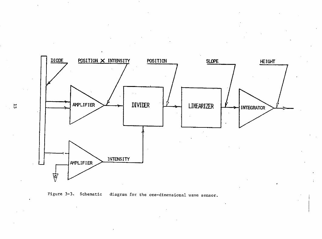
DIODE POSITION X INTENSITY POSITION SLOPE HEIGHT
DIVIDER LIMEARIZER IINTEGRATOR
APLIFIR INTENSITY
Figure 3-3. Schematic diagram for the one-dimensional wave sensor.

differential transformer (dcdt) which drives the error circuitry. The loud-
speaker, dcdt, and error circuit comprise a feedback-controlled electro-
mechanical transducer with controllable response characteristics. The
power amplifier is of a clmplementary-symmetry transistor design such
that one can obtain full power response down to dc. The laboratory set-up is
shown in Figures 3-4 and 3-5.
3.2 Error Analysis Due to Surface Motion
Since the wave surface is constantly in motion, the reflection point
is moving also, hence error may be introduced in the measurement process.
To calculate the order of the error induced in this way we first examine
the case of a single train of waves where the surface elevation t(x,t) is
given as
C(x,t) = a sin(kx - at) = a sin X (3-7)
Let the distance between the mean water surface to the diode be H, then the
instanteneous distance will be
h(t) = H + a sin X (3-8)
To the approximation of equation (3.6a), we have the apparent surface
elevation t*(x,t) as
*(xt)= (H + a sin X) ak cos X dx2
a sin X + - cos 2X (3-9)
which results in an error on the order of
C aa a4H
In our study, a = 0.2 cm, H = 100 cm. and the error is about 0.05%.
In the case of random wave field, the phase speed is hard to determine;
therefore the surface elevation spectrum will have to be derived from the
expression for the surface slope spectrum. Let the surface of the random wave
16

-m m
Figure 3-4. Laboratory set-up of the capillary-gravity wave tank.

est avala
e
copy
4).I)
0I0 I*i
0o
18
0d+,r~-4
C-
Lfd

field be expressed as
(2, t) = f dA(k,n) eiX (3-10)
k n
with dA(k,n) as a complex valued random function which is related to the
spectrum X(k,n) by
dA(k,n) dA*(kl,nl) = X(k,n) if k = 1, n = n,
= 0 if k A k I , n / n1 (3-11)
The surface slope will be
V (x, t) = ik dA(k,n) e . (3-12)
k n
Thus the surface slope spectrum is
S i(k,n) = ffkik X(,n) dk dn (3-13)
k n
where k., kj are the components of wave number in the ith and jth direction.
For a one dimensional case ki = k. = k and
S(k,n) = f 1k2 X(k,n) dk dn (3-14)
k n
Again, if the distance between the mean water level to the diode is given
by H, the excursion of the light spot on the diode is
E(x,t) = H + f fdA(k, n) e i X f AA (,n) eiX (3-15)
k n k n
The correlation function of this random position is
19

Z(x, t) *(x + ', t + T)
= H + dA(g,n) e x i k dA( k1 ,nl1 ) elX 1
kn k n If~f f1 ~
(3-16)
SH + dA* 2 ,n2 ) eX2 f f -i k 3 dA*(k,nl)e - i X3
n n3
After some algebra, we have
E(x,t).E( + Z, t + t)
H k= H2 kik X(n) 1 1 3- i
k n k n
(3-17)
* X(Q,nl) d k1 dn1 dk dn
Comparing (3-17) with the true surface slope spectrum, we have an error of the
order of
3 k2 X(k,n I) dk dn1 = 0 ) (3-18)
k n~1 -1
Although, the result is wave number dependent, its magnitude is small2 2if H >> 2 which was the case in the set-up for experimental study.
3.3 Results of the Measurements
As indicated in Eq. (3-6) one must know the phase velocity before quanti-
tative amplitude measurements on single trains of waves can be obtained. In
theory, at least, it is a straightforward matter to obtain the phase velocity
c from c = fA, as A can be measured experimentally and f, the wave (plunger)
frequency, is known. However, for the short wavelengths encountered small
20

errors in measured wavelength will result in relativeiy large errors in
phase velocity. In view of this a general dispersive relationship was
sought in an attempt to minimize experimental scatter. In an exhaustive
set of trials, f vs X dat- were obtained which permitted the construction
of a plot of phase velocity as a function of wave period. Using small
amplitude wave theory the surface tension for this data was calculated to
be 63 dyne/cm. A measurement of the static surface tension with a du Noiy
tensiometer confirmed the low value of surface tension obtained from the
dispersive relationship. The wavetank was cleaned and refilled with tap
water. The static surface tension was measured and found to be 70 dyne/cm.
From careful wavelength measurements and the small amplitude dispersive
relationship the surface tension (dynamic) was calculated. A surfactant
(Woolite) was added and the experiment was repeated. The static surface
tension was measured with the tensiometer and found to be 30 dyne/cm, and
again with in + 1.5 dyne/cm the surface tension calculated from the dispersive
relationship was in agreement. These experiments were taken to indicate
that the correct value of surface tension could be obtained from either a
measurement of the frequency and wavelength of the waves and use of the
dispersive relation or by a simple static measurement of the surface tension.
Similar results have been reported by Davies and Vose (1965) for most liquids
including water; however, McGoldrick (1970) has reported values of the dynamic
surface tension 10% lower than the static value for water. After this
confirmation of the equivalence of results from either method the phase velocity
was subsequently obtained from static surface tension measurements and direct
computation using the dispersive relationship with periodic verification by
direct measurements of the wave length.
Preliminary trials of the optical system consisted of the measurement of
peak to trough amplitudes of arbitrarily selected gravity-capillary waves
in the range of 6 to 18 Hz. The amplitude (computed as described in Sec. 3.1)
as measured by the optical system was compared to the amplitude as measured
by a capacitive wave he :.ht transducer similar to that developed by McGoldrick
(1971). The present wa height transducer consisted of a No. 30 hypodermic
needle (diameter 0.224 mm) which, when immersed in the water surface, controlled
the amplitude of a 455 kHz square-wave oscillator. After suitable amplitude
demodulation, an analog voltage proportional to the needle immersion depth was
obtained. For the longer wavelengths (greater than approximately 5 cm) the two
21
systems had identical responses, but for shorter wavelengths the optical
system indicated predominately higher values of peak to trough amplitude
(c.f. Fig. 3-6).
To determine which instrument was in error a direct geometric measure-
ment of wave amplitude was made. This was accomplished by using a sinusoidal
surface wave which was obtained by adjusting the amplitude, frequency and
position of the wave generator. For a sinusoid of peak to trough amplitude,
a, the maximum slope is ak/2. The maximum angle swept by the refracted beam
was determined by measuring with a scale the swept length of the beam on a
plane a known distance from the water surface. The value of ak was then
calculated from the relation
ak = swept length/distance of water to plane
Then a measurement of wavelength, and thus k, permitted a separate measurement
of amplitude for this special case. The amplitude measured in this manner
closely agreed with that obtained by the optical system and this established
the measured amplitude as a tentative standard.
With this standard, constant peak to trough amplitude surface waves were
generated at varying wavelengths. A summary of the response is presented in
Fig. 3-6.
In an attempt to explain the observed rolloff in the response of the
wave height probe at the shorter wavelengths it was hypothesized that the
meniscus did not maintain a constant height on the probe. Another way of
expressing this is to say the meniscus exhibited a hysteresis effect and did
not slide on the probe as if it were a rigid body. This hypothesis was
investigated experimentally by the forced immersion of the probe into still
water. While attached to the wave generator shaft (plunger wedge removed)
the probe was driven with a number of waveforms, symmetrical and non-symmetrical,
over a range of frequencies from 0.2 to 40 Hz at various amplitudes. Under all
conditions imposed,.the immersion depth as measured by the probe, compared
within 10% to that of the wave generator shaft displacement as indicated by
the dcdt position transducer. It was therefore concluded that the meniscus
maintains a nearly constant height on the probe with respect to the instantan-
eous position of the level surface. The small attenuation observed was in-
sufficient to explain the rolloff presented in Fig. 3.6.
22

1.3 WAVE AMPLITUDE
0 0.5 mm1.2 1.0 mm
1.2.0 1.5 mm
1.1 0 2.0 mm
d0- 0.9 -
0.8 oo
0.7 '&0
0.6 o 0
0.5 I I .
10 9 87 6 5 4 2
WAVELENGTH, cm
Figure 3-6. Ratio of wave amplitudes as measured by the probe (a ) to that measured by the optical
method (ao). The light beam is 0.30 mm in diameter.

An alternate explanation for the reduced probe response at the shorter
wavelengths was postulated to be a lack of spatial resolution. At the
shorter wavelengths a higher degree of resolution becomes necessary to avoid
an averaging of the amplitude structure. It was therefore hypothesized that
if the effective size of :he probe resulting from an attached meniscus was
much larger than that of the unwetted probe, the resolution would be limited
by this effective probe diameter. To check this hypothesis the diameter of
the light beam was gradually increased from a nominal 0.5 mm to a diameter
of approximately 6 mm. With this 6 mm beam diameter (and consequently reduced
spatial resolution) the response of the optical system and the capacitive
wave height probe were nearly identical. Figure 3-7 presents a plot of the
ratio of peak to trough amplitudes as measured by the wave height probe to
that obtained by the optical system.
Within the bounds of experimental error and the exception of a small
unexplained dip in the probe response at X = 2 cm, the two systems had a
comparable response. It is therefore concluded that the observed rolloff of
the wave height probe at short wavelengths was due to a lack of spatial
resolution. For the No. 30 needle used the effective diameter of the attached
meniscus was assumed to be that of the enlarged light beam and thus approximately
5-7 mm.
The problem of insufficient spatial resolution has been considered by
Cox (1958) for his optical system. When one substitutes the experimentally
determined effective probe diameter of 5-7 mm for the sensor diameter in his
analysis a response which closely parallels the data of Fig. 3-7 is predicted.
A theoretical means of estimating effective probe diameters, and hence
the resolution, can be obtained by an analysis of static menisci on circular
cylinders. One observes from meniscus profiles, calculated numerically and
verified experimentally by White and Tallmadge (1965), that an effective
probe diameter of 6 mm would correspond to the diameter of the meniscus
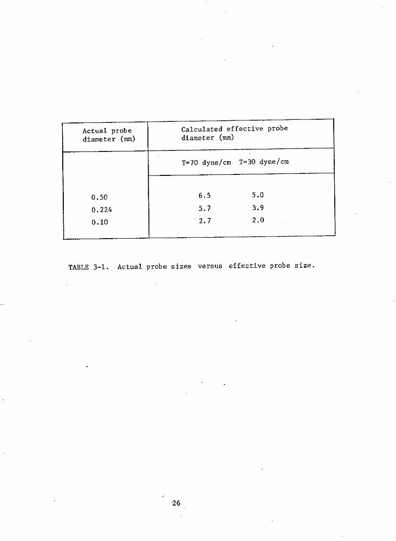
where the height is 1 the maximum height. Using this criterion Table 3-1
presents calculated effective diameters for probes roughly double and half
the diameter used in this investigation.
It is clear from Table 3-1 (and casual observations of probes in water)
that the meniscus diameter is much larger than the probe itself. Since the
effective sensor diameter presented by the meniscus is a rather weak function
of probe diameter this points out that lack of spatial resolution is an
24

1.40
1.30
1.20
.00 0 00B d ,oo ___- ---0 o 0
0.90-
0.80
0.70
0.60
9 8 7 5 4 3 2
WAVE LENGTH IN CM.
Figure 3-7. Ratio of wave amplitudes when the light beam diameter is 6
mm.
Actual probe Calculated effective probe
diameter (mm) diameter (mm)
T=70 dyne/cm T=30 dyne/cm
0.50 6.5 5.0
0.224 5.7 3.9
0.10 2.7 2.0
TABLE 3-1. Actual probe sizes versus effective probe size.
26

inherent problem with this class of wave detectors. This would appear to be
a serious restriction of the usefulness of these wave height probes where the
measurement of small, short waves is desired.
In passing it must be noted that the optical system described responds
to general two-dimensional surfaces as the light beam is refracted in relation
to the total surface slope. As a consequence, when the refracted light beam
is projected on a flat surface one visually observes a two-dimensional pattern,
similar to a Lissajous figure, if a two-dimensional surface disturbance is
scanned. For the special case of one-dimensional wave trains, the pattern
degenerates to a straight line. When transverse waves are present the pattern
opens into a two-dimensional figure. This feature is especially useful for
detecting low amplitude cross (transverse) waves which are frequently observed
to be associated with plunger type wave generators. In one-dimensional wave
studies this form of distortion is much more difficult to detect with wave
height probes.
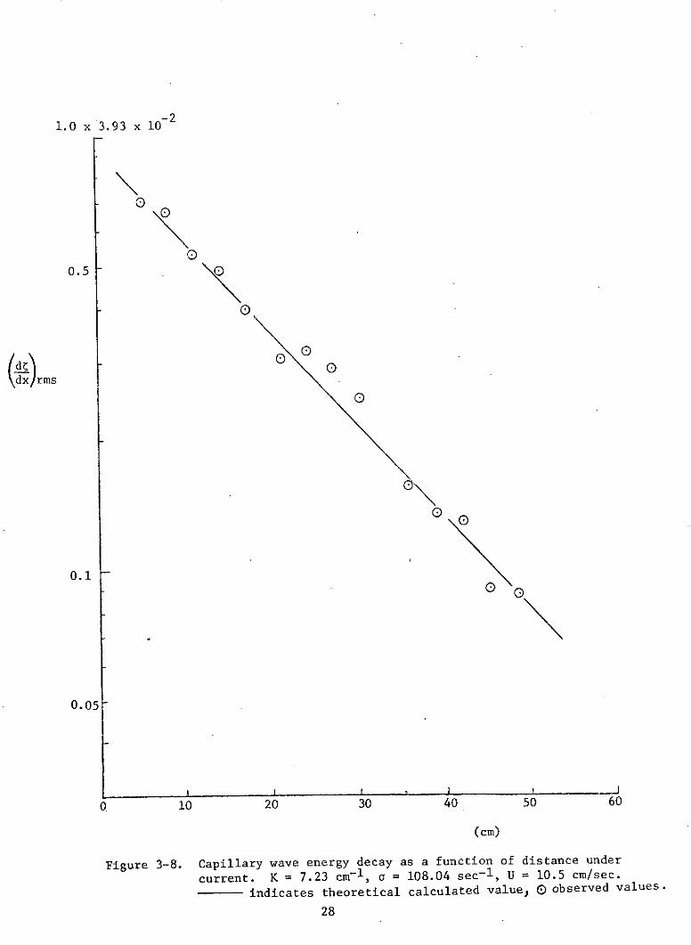
Having established the calibration, we moved on to measure the decay rates
of the energy density of two capillary waves. The rate of energy decay is
calculated according to
dE 1 dE = 2yk 2 (3-19)dt C dX C
g g
where y is the surface tension force. The calculated and measured results
are shown in Figures 3.8 and 3.9.
The final measurement using the present system was on current velocity.
A pump was connected to the tank to generate a variable current anywhere
between + 20 cm/sec. The current velocity was independently measured by a
hot film anemometer and three sets of test were conducted with two of the
tests for waves traveling with the current and one for waves travelling
against the current. The results are summarized in Tables 3-2, 3-3, and
3-4.
3.4 Additional Laboratory Work
Since the final test of the theory will not be conducted in the capillary
wave range alone, a wind-wave channel with the dimensions of 2' x 3' cross-
section and 50' long has been constructed through the coastal research program
supported by the North Carolina State Government at NCSU. The blower on the
27
-21.0 x 3.93 x 10
0
0.5 0
0
(d(dx/ rms
0.1
0.05
I I I
0 10 20 30 40 50 60
(cm)
Figure 3-8. Capillary wave energy decay as a function of distance under
current. K = 7.23 cm-1, a = 108.04 sec-1, U = 10.5 cm/sec.
indicates theoretical calculated value, O observed values.
28

1.0 x 3.93 x 102
0.50"0o
rms
0\
0.05
0 10 20 30 40 50 60
(cm)
Figure 3-9. Capillary wave energy decay as a function fo distance under
current. K = 6.37 cm-1, o = 78.80 sec
- 1 , U = 12.37 cm/sec.
- indicates theoretical calculated value. Oobserved values.
29

Measured Calculated
measured
Period Wave length Current Current
(ms) (cm) (cm/sec) (cm/sec) Ucalculated
Ucalculated Umeasured
24.860 0.878 11.0 9.89 1.112
24.866 0.903 10.0 11.06 0.904
24.868 0.924 11.5 12.08 0.961
24.864 0.859 9.0 8.98 1.002
28.575 0.993 11.5 10.15 1.133
28.574 0.999 12.0 10.37 1.157
28.635 0.972 12.0 9.23 1.300
28.606 1.010 14.0 10.84 1.292
28.604 0.998 11.0 10.30 1.068
25.125 0.860 11.0 8.66 1.270
25.358 0.927 11.5 11.50 1.000
25.905 0.932 11.5 11.76 0.978
Average = 1.097
TABLE 3-2. Current measurements through wave kinematics Case 1.
30

Measured Calculated
measured
Period Wave length Current Current
(ms) (cm) (cm/sec) (cm/sec)
measured calculated l
27.970 0.984 11.5 10.53 1.092
24.940 0.883 11.5 10.02 1.148
23.318 0.836 10.0 10.04 0.996
21.420 0.768 9.5 9.37 1.014
28.016 0.964 9.0 9.65 0.941
27.880 0.966 9.0 9.92 0.907
35.590 1.186 9.0 9.63 0.935
30.470 1.007 9.0 8.52 1.056
27.276 0.942 9.5 9.62 0.988
28.507 0.903 5.0 6.44 0.776
31.000 0.940 5.0 5.36 0.933
32.570 1.116 10.2 10.30 0.991
29.199 0.989 10.5 9.25 1.135
26.359 0.910 9.0 9.33 0.965
Average = 0.991
TABLE 3-3. Current measurements through wave kinematics Case 2.
31

Measured CalculatedUmeasured
Period Wave length Current Current
(ms) (cm) (cm/sec) (cm/sec) UU U calculatedmeasured calculated
62.170 0.757 -14.5 -14.33 1.012
.66.440 0.982 - 9.0 - 9.89 0.910
58.820 0.894 - 9.0 -10.10 0.882
55.300 0.859 - 9.0 -10.00 0.900
62.170 0.695 -14.5 -16.24 0.893
62.195 0.941 - 8.5 - 9.80 0.867
66.621 0.859 -11.5 -12.69 0.906
58.825 0.925 - 9.0 - 9.32 0.965
55.325 0.854 -10.0 -10.17 0.983
58.159 0.869 -11.0 -10.55 1.043
58.158 0.735 -14.0 -14.25 0.982
58.159 0.826 -11.0 -11.70 0.940
66.441 0.900 -11.0 -11.70 0.940
-80.415.-.- ,,0986 .. -11.5 -12.38 0.929
99.612 1.143 -11.5 -12.38 0.929
100.627 1.143 -11.5 -12.51 0.919
100.573 1.522 - 8.0 - 7.90 1.013
75.648 1.165 - 8.0 - 8.39 0.954
54.702 0.918 - 8.0 - 8.31 0.963
54.590 0.926 - 8.0 - 8.08 0.990
Average = 0.990
TABLE 3-4. Current measurements through wave kinematics Case 3.
32

tank is capable of generating a wind up to 80 knots. A variable speed pump
will be connected to the tank to generate current together with wind and
waves. This channel will be used to check the theoretical results in a near
natural environment. Since wind waves are highly irregular, cross tank
components will become increasingly important. The waves will be quasi-
two-dimensional. Under this condition, the present system described in
Sections 3.1 and 3.3 will become inadequate, and a new electronic system
is being designed and constructed in our laboratory. The construction is
still unfinished at the present moment. The detail of the system is
described as follows.
To analyize the two-dimensional signal resulting from the wind-wave
field, an array of light sensitive diodes was used, thirty-two Vactec S150LB
diodes for each dimension, allowing two diodes for each of the sixteen steps
in each dimension as shown in Figure 3-10. Since the laser beam is, at any
one instant of time, a single dot, only one strip at a time in each array
will be illuminated by the dot. The location of the dot gives the slope in
x and y directions respectively. As the dot moves, there will also be times
when the dot crosses the gap between strips of diodes. Thus the electrical
output from each array will be a burst of voltage, typically about 70 mv,
when the dot of light is on any given diode, with zero output for the gaps
between the strips. To convert this output into data that are more readily
analyzed, an array of integrated circuits was employed.
Initially, thirty-two voltage comparators, MC1710, are divided into
two groups of sixteen. Each of the sixteen monitors one of the arrays of
diodes and each strip in the array is therefore continuously monitored for
output. The function that the MC1710 comparators perform is to compare
voltages with a reference voltage that is adjustable by means of a 10K Ohm
trim pot and each is therefore tuned to the output level of its particular
pair of diodes on the strip it monitors. The typical output differs slightly
from 70 my due to diode manufacturing variations, thus each comparator is tuned
to recognize the dot when laser light strikes the diode strip and causes a
voltage greater than its reference. The comparator then switches "on", supplying
one NAND gate in a N7400A package with about 3.2 volts. The NAND gate inverts
the signal and switches on one of the FLIP-FLOPS in a dual package, US7476A.

y Y x
X
Diodes
-Beam Splitter
Signal
Figure 3-10. Arrangement of the Photo diodes for two-dimensional waves.Figure 3-10. Arrangement of the Photo diodes for two-dimensional waves.
Unlike the comparators or NAND gates, the FLIP-FLOPS will remain "on"
supplying about 3.5 volts until instructed to turn "off". This feature
of the FLIP-FLOPS enables the final output to remain at that level while
the dot crosses the gaps between strips, and no incoming signal is present.
To prevent more than one FLIP-FLOP in each array division from being on at
the same time (which would indicate the dot was at two places at the same
time), part of the initial output of the FLIP-FLOP turns on a NOR gate, in
a-N7402A package, which in turn switches "off" (through the reset input)
the FLIP-FLOPS corresponding to the step on either side of the location of
the dot. Thus the final output of the FLIP-FLOP corresponds to the location
of the laser dot on the diode. Since all the FLIP-FLOP outputs are the same,
typically 3.5 volts, these outputs are fed through precision resistors changing
in value from 2K to 16K in 1K steps. Each 1K step corresponds to a different
diode strip, and thus when fed into a MC1741 OP AMP, are amplified differentially.
The final output then appears as "steps" in close approximation to the
continuous slope. For smaller steps, and thus more accuracy, only the
addition of more diode strips and electronics to monitor them is necessary.
To summarize the description, the original quantized output of the diodes
is processed electronically into slope information as shown schematically in
Figure 3.11. To make this electronic analysis of the signal, the following
supply voltages were needed-:
MC1710 Comparators --- + 14v, - 7v, 80 my reference
N7400A QUAD 2-INPUT NAND GATE
US7476A DUAL J-K FLIP-FLOP + 5v
N7402A QUAD 2-INPUT POS. NOR GATE
MC1741, OP AMP + 15v
To supply these voltages, an MC1561R was used for the + 15v. and 80 mv,
another MC1561R for the + 14v and MC1463R for the - 7v, and a ZN3055 power
transistor working with a 1N4733 Zener diode for the + 5v. A detailed circuit
diagram is given in Figure 3.12.
35

COM PON ENTSNOR GATES
D\ODEs COM PARATORS NARD 6tATE-S OP AM PFLIP-FLOPS
r 1 I - - -l --.-- -I
I i I I I
FINAL
DIODE 32VSINAL
70 MYV
TIME
FSNAL
Figure 3-11. Schematic diagram of the signal processing.

L UT -RAMA _4v
A : VAcT6 DiDIES
s.12.tCa T
C ... l t N7 4 Aj "I. - I Q,, 6A te
1N 6 R 910$8 -oP5
-3 1 1 43
.=..4 ,0l 0,- ' -/t pig: 2Avor
I -2o-3o t
" I
L-- 0,
to *6 o 6 9o
L 7-K N 473
-. -i- i R-
Figure 3-12. Circuit diagram for the two-dimensional wave sensor. |best available copy.
37
it, 4 F 7 Q 1 11 111I1 Q -o- 'Ask11111 00
=T tIrI I~*C4-
Rerdue foFigre3-2.Cicut iara fr te wodienioalwae enor 6 f valalecov
37r
4.0 SUMMARY AND DISCUSSION
The feasibility of monitoring surface current through wave observation
by remote sensing technique was established in theory and also in preliminary
experimental tests. The accuracy of the method, under laboratory controlled
condition, is comparable to any other in situ measurements. Two different
approaches were discussed. For the experiment, the kinematic approach was
verified for a single train of gravity-capillary waves. The final decision
for field adoption will, of course, depend on the kind of instruments available
at that time.
For the laboratory studies, an optical wave slope detection system
capable of fine spatial resolution and high frequency response has been
developed. The system, which employs the refraction of a narrow beam of
light at the air-water interface, is ideally suited to the study of short
gravity-capillary waves (X < 5 cm) as spatial resolution is controlled by
the light beam diameter, frequency response by the electronics employed,
and no extraneous surface distortion is generated. For the special case
of a single train of waves propagating with a known phase velocity, the
s-lope signal can be integrated (electronically in the present case) to obtain
the wave amplitude as it passes a fixed observation point. Moreover, the
technique is applicable to the study of waves on a current, providing the
total phase velocity (in laboratory coordinates) is used in the slope to
amplitude calculations. The accuracy of the present amplitude measurement
technique is largely dependent on the accuracy to which the phase velocity
is known. Experiments indicate that the surface tension calculated from
measurements of wave frequency and wavelength agree to within + 1.5 dyne/cm
with that measured by a du NoUy tensiometer, and thus small amplitude wave
theories can be used to calculate phase velocity once the (static) surface
tension has been measured. In the absence of a "standard laboratory wave"
the overall accuracy .of the optical slope/amplitude detection system must be
estimated from the total instrumentation uncertainty. For the measurement
of waves with peak slopes less than 0.5 the present system should give wave
slopes accurate to within 5%. The total amplitude error is that of the
combined slope and integrator error multiplied by the uncertainty in the
phase velocity. For the present investigation this total error is estimated
to be less than 10%.
38

Although the preliminary results are encouraging, considerably more
work remains until an operational routine can be established. In order
to achieve such an ultimate goal, the following studies have to be carried
out.
(a) Additional Theoretical Analysis
The theoretical study will be used as a guide for planning both
in the laboratory and in the field. The more we know about the
topographical features of a random wind-wave field, the more we can
detect the influence of current on waves. The theoretical studies
will include both kinematics and dynamics of wind generated waves over
all wave number-frequency range. Although in the ocean most energy
is contained in the gravity wave range which has also held the central
attention of oceanographers, the gravity-capillary waves or even the
pure capillary waves are important in radar remote sensing problems.
(b) Additional Wave Tank Studies
A wave tank study is the first step prior to field tests. In
order to simulate the natural environment better, wind generated
waves will be used next. The two-dimensional wave sensor will be
employed to make wave spectrum analysis. Such observations can be
used to check the validity of theoretical results and also provide
guidance for field instrument design.
Table 4-1 is given as a summary of the status of the study. Completed,
planned and in-progress efforts are listed for quick reference.
39

TABLE 4-1. Summary of work in progress and future plans.
GRAVITY WAVES GRAVITY-CAPILLARY WAVES CAPILLARY WAVES
REGULAR RANDOM REGULAR RANDOM REGULAR RANDOM
THEORETICAL EXISTING FINISHED FINISHED PLANNED IN PROGRESS IN PROGRESSKINEMATICSTUDY 2D KINEMATIC 2-D 2D
D currents currenti1D -D 1-D
PLANNED PLANNEDRANDOM DYNAMICSCURRENT
i-----i---------- --- "------------__--_--'--- _ -
! EXPERIMENTAL EXISTING PLANNED IN PROGRESS PLANNED IN PROGRESS PLANNED
STUDY 1-D current (1-D current)

REFERENCES
Cox, C. S. (1958):Measurements of Slopes of High-Frequency Wind Waves
(J. Mar. Res., 16, 199-225)
Cox, C. S. and Munk, W. H. (1954)Measurements of the Roughness of the Sea Surface from Photographs
of the Sun's Glitter
(J. Optical Soc. Amer., 44, 838-850)
Davies, J. T. and Vose, R. W. (1954)
On the Damping of Capillary Waves by Surface Films
(Proc. Roy. Soc., A, 286, 218-234)
Francis, J. R. D. and Dudgeon, C. R. (1967)
An Experimental Study of Wind Generated Waves on a Water Current
(Q. J. Roy. Meteor Soc., 93, 247-253)
Huang, N. E.; Chen, D. T.; Tung, C. C. and Smith, J. R. (1972)
Interactions between Steady Non-uniform Currents and Gravity Waves
with Applications for Current Measurements
(J. Phys. Oceangraphy, 2, 420-431)
Hulburt, E. D. (1934)
The Polarization of Light at Sea
(J. Optical Soc. American, 24, 35-42)
McGoldrick, L. F. (1970)
An Experiment on Second-Order Capillary Gravity Resonant Wave Interactions
(J. Fluid Mech., 40, 251-272)
McGoldrick, L. F. (1971)
A Sensitive Linear Capacitance-to-Voltage Converter, with Applications
to Surface Wave Measurements
(Rev. Scientific Inst., 42, 359-361)
Phillips, 0. M. (1966)The Dynamics of the Upper Ocean
(Cambridge University Press, pp. 261)
Plate, E. and Trawle, M. (1970)A Note on the Celerity of Wind Waves on a Water Current
(J. Geophys Res., 75, 3537-3544)
Schooley, A. H. (1954)A Simple Optical Method for Measuring the Statistical Distribution
of Water Surface Slopes
(J. Optical Soc. Amer., 44, 37-40)
White, D. A. and J. A. Tallmadge (1965)Static Menisci on the Outside of Cylinders
(J. Fluid Mech., 23, 325-336)
41