Embed Size (px)
Citation preview

Southern Methodist University Southern Methodist University
SMU Scholar SMU Scholar
Mechanical Engineering Research Theses and Dissertations Mechanical Engineering
Spring 2020
Critical Point Identification In 3D Velocity Fields Critical Point Identification In 3D Velocity Fields
Mohammadreza Zharfa [email protected]
Follow this and additional works at: https://scholar.smu.edu/engineering_mechanical_etds
Part of the Other Mechanical Engineering Commons
Recommended Citation Recommended Citation Zharfa, Mohammadreza, "Critical Point Identification In 3D Velocity Fields" (2020). Mechanical Engineering Research Theses and Dissertations. 27. https://scholar.smu.edu/engineering_mechanical_etds/27
This Thesis is brought to you for free and open access by the Mechanical Engineering at SMU Scholar. It has been accepted for inclusion in Mechanical Engineering Research Theses and Dissertations by an authorized administrator of SMU Scholar. For more information, please visit http://digitalrepository.smu.edu.

CRITICAL POINT IDENTIFICATION IN 3D VELOCITY FIELDS
Approved by:
_______________________________________
Prof. Paul S. Krueger
Professor of Mechanical Engineering
___________________________________
Prof. Ali Beskok
Professor of Mechanical Engineering
___________________________________
Prof. Eli Olinick
Associate Professor of
Engineering Management
and Information Systems

CRITICAL POINT IDENTIFICATION IN 3D VELOCITY FIELDS
A Thesis Presented to the Graduate Faculty of
Lyle School of Engineering
Southern Methodist University
in
Partial Fulfillment of the Requirements
for the degree of
Master of Science in Mechanical Engineering
by
Mohammadreza Zharfa
B.S. in Mechanical Engineering,
University of Tabriz, 2008
May 16, 2020

Copyright (2020)
Mohammadreza Zharfa
All Rights Reserved

iv
ACKNOWLEDGMENTS
I would like to express my sincere appreciation to SMU for the research assistantship I
received during the study. I would like to express my sincerest appreciation to all those people
who have supported me either physically or morally throughout this study. I am fully grateful to
my supervisor Prof. Paul S. Krueger for his unique guidance, encouragement, support, criticism
and invaluable supervision. It was an honor for me to study with him throughout my graduate
education. I should also thank Prof. Eli Olinick and Prof. Michael Hahsler for their help in
developing the algorithm in this work.
I would also like to express my thanks to my friends: Bin Xia, Matt Saari, Travis Mayberry
and Nicholas Davis for their support. I have been very lucky to share unforgettable moments in
Experimental Fluid Mechanics Lab with good friends.
The material in this thesis is based on work supported by the National Science Foundation
under Grant No. 1557698. This support is gratefully acknowledged.

v
Zharfa, Mohammadreza B.S, University of Tabriz 2008
M.S, Middle East University 2015
Critical Point Identification In 3D Velocity Fields
Advisor: Professor Paul S. Krueger
Master of Engineering conferred May, 16, 2020
Thesis defended April, 10, 2020
Classification of flow fields involving strong vortices such as those from bluff body wakes
and animal locomotion can provide important insight to their hydrodynamic behavior. Previous
work has successfully classified 2D flow fields based on critical points of the velocity field and
the structure of an associated weighted graph using the critical points as vertices. The present work
focuses on extension of this approach to 3D flows. To this end, we have used the Gauss-Bonnet
theorem to find critical points and their indices in the 3D velocity vector field, which functions
similarly to the Poincare-Bendixon theorem in 2D flow fields. The approach utilizes an initial
search for critical points based on local flow field direction, and the Gauss-Bonnet theorem is used
to refine the location of critical points by dividing the volume integral form of the Gauss-Bonnet
theorem into smaller regions. The developed method is cable of locating critical points at sub-grid
level precision, which is a key factor for locating critical points and determining their associated
eigenvalues on coarse grids. To verify this approach, we have applied this method on sample flow
fields generated from potential flow theory and numerical methods.
vi
TABLE OF CONTENTS
ACKNOWLEDGMENTS ............................................................................................................. iv
TABLE OF CONTENTS ............................................................................................................... vi
LIST OF FIGURES ................................................................................................................. viii
LIST OF TABLES ..................................................................................................................... ix
CHAPTER 1 .................................................................................................................................. 1
INTRODUCTION..................................................................................................................... 1
1.1 Motivation ......................................................................................................................... 1
1.2 Critical Point Detection..................................................................................................... 6
1.3 Objectives ......................................................................................................................... 7
CHAPTER 2 .................................................................................................................................. 8
METHODOLOGY OF IDENTIFYING CRITICAL POINTS: ALGORITHM ................ 8
2.1 Localization and Identification of Critical Points in 2D Vector Fields ............................ 8
2.2 Localization and Identification of Critical Points in 3D Vector Fields .......................... 15
2.3 The 3D Algorithm ........................................................................................................... 18
CHAPTER 3 ................................................................................................................................ 27
IMPLEMENTATION AND RESULTS ............................................................................... 27
3.1 Implementation ........................................................................................................... 27
3.2 Vector fields for Algorithm validation ....................................................................... 31

vii
3.3 Results and discussion ................................................................................................ 36
CHAPTER 4 ................................................................................................................................ 41
CONCLUSION ....................................................................................................................... 41
REFERENCES ............................................................................................................................ 43
APPENDIX 1 ............................................................................................................................... 47
APPENDIX 2 ............................................................................................................................... 49

viii
LIST OF FIGURES
FIGURE PAGE
1-1 CLASSIFICATION OF CRITICAL POINTS IN 2D ........................................................................................... 2
1-2 CONCEPT OF FEATURE FIELDS ..................................................................................................................... 4
2-1 POINCARE-INDEX CALCULATION IN 2D VECTOR FIELD ......................................................................... 9
2-2 MAPPING OF VECTORS AROUND DIFFERENT POINTS, I) A NODE, II) NO-CRITICAL POINT, III) A
SADDLE ............................................................................................................................................................ 11
2-3 FLOW ORIENTATION ANGLES AT FOUR DIFFERENT POINTS ............................................................... 13
2-4 ILLUSTRATION OF Θ_M AT DIFFERENT POINTS ...................................................................................... 14
2-5 INDEX NUMBER DEFINITION FOR A REGULAR POINT (A) AND A CRITICAL POINT (B) ................. 17
2-6 ITERATION MECHANISM IN STEP 1 ............................................................................................................. 19
2-7 FREQUENCY DISTRIBUTION PATTERN FOR A NON-CP (LEFT) AND A CP (RIGHT) .......................... 21
2-8 ITERATION MECHANISM IN STEP 2 ............................................................................................................. 23
2-9 THREE POSSIBLE COMPONENTS OF Θ_P .................................................................................................... 24
3-1 VECTOR SAMPLING OVER A CUBE (A) AND POSITIONS OF R AND S ON EACH FACE .................... 29
3-2 GAUSSIAN WEIGHTED INTERPOLATION TO MATRIX A AT CENTROID LOCATION ........................ 31
3-3 ENTIRE 3D POTENTIAL FLOW OVER A SPHERE (A), CROSS SECTION OF THE SAME FLOW FIELD
WITH SHOWN CRITICAL POINTS BY RED DOTS (B) .............................................................................. 32
3-4 RANKINE BODY FLOW WITH RELATIVELY SMALL CRITICAL POINT SPACING (RED DOTS
REPRESENT CRITICAL POINTS) .................................................................................................................. 33
3-5 A LORENTZ ATTRACTOR STATE FLOW DOMAIN WHICH SHOWN CRITICAL POINTS………...……35
3-6 HISTOGRAM PLOTS FROM IMPLEMENTATION OF STEP 1 ON THREE DIFFERENT POINTS B
(CRITICAL POINT) AND A, C (NON-CRITICAL POINT)…………………………………………………36
3-7 OUTCOME OF FLOW ORIENTATION TEST (STEP 1) ON THE ENTIRE FLOW…….…………………….37
3-8 FLOW ORIENTATION SCAN (A), GAUSS-BONNET INDEX EVALUATION (B) ON THE FLOW FIELD
SHOWN IN FIGURE 3-4…………………………………………………………………………….………..38
3-9 CORRESPONDING ISOSURFACE PLOTS AND EIGEN VALUES OF SPIRAL SADDLE POINT (A) AND
NSS POINT (B) OF A LORENTZ ATTRACTOR FLOW FIELD…………………………………...……….39

ix
LIST OF TABLES
TABLE 2-1 SUMMARY OF 2D CRITICAL POINT ALGORITHM AND THE 3D EXTENSION.. ....................... 8

1
CHAPTER 1
INTRODUCTION
1.1 Motivation
A variety of fluid flows, such as those generated by bluff bodies or animal locomotion, are
characterized by wake flows with coherent vortical patterns [1]. Understanding of the dynamic
behavior of such flows is of great interest for many industrial and biological applications. For
example, it is beneficial to understand hydrodynamic forces on a bluff body or swimming
efficiency of animal locomotion, which are related to the flow development in the wake of these
flows.
Usual ways to understand flow patterns and the associated physics are typically based on
qualitative flow visualization [3] or qualitative assessment of patterns observed in quantitative
flow field measurements. Such qualitative observations can be related to flow dynamics through
measurement of overall forces, as well as distribution of surface pressure and acceleration.
However, qualitative approaches are subjective and it is difficult to apply them to complex flows
as the number of degrees of freedom are higher for these types of flows.
To move toward objective methods for characterizing flow patterns, it is necessary to
utilize quantitatively identifiable flow features. Critical points of the flow velocity field are useful
in this regard as they are related to structural patterns in the flow streamlines. and can provide a
reduced order representation of the essential flow features that can be used for quantitative
comparison of two flow fields [5].
Critical points are those points where the vector magnitude in a vector field disappears and
the determinant of the gradient of velocity vector (velocity gradient tensor) is not equal to zero
(𝑑𝑒𝑡(∇𝐮) ≠ 0). These points can be categorized according to the behavior of adjacent tangential

2
curves. The tangential curves, which end at critical points, are important as they describe how the
vector field behaves around these points [6] and the local behavior of these curves is determined
by the eigenvalues of the velocity gradient tensor of the vector field (∇𝐮 for vector field 𝐮) at the
location of the critical point. Consequently, critical points can be classified based on their
eigenvalues.
Figure 1-1 shows classifications of critical points according to corresponding eigenvalues
for a two-dimensional vector field. R1 and R2 indicate the real parts of the eigenvalue of the
Jacobian and I1 and I2 are the imaginary parts. We can infer that positive or negative real part of
the eigenvalues indicates that the critical point is attracting or repelling, respectively.
One way to compare flow field patterns is to directly consider the critical points embedded
in the flows. Then comparing the flows reduces to a set of points and the similarity between two
Figure 1-1 - Classification of critical points in 2D
Figure 2-1 - Classification of critical points in 2D

3
sets of points can be measured by definition of distance between these point sets in a metric space
[7]. Eiter and Mannila [7] extend a distance function between points to a distance function or
metric between point sets. They also investigated different approaches for this, and have analyzed
the computational complexity of the resulting functions.
Lavin et al. [8] used the concept of earth mover’s distance introduced by Yossi et al. [9]
for image retrieval for large image data bases. The earth mover’s distance (EMD) is a distance
measurement between two probability distributions over region. If we assume each distribution
can be represented as a pile of dirt, the metric is the minimum cost of turning one pile (distribution)
into the other pile. The cost is the amount of dirt to be moved times the distance. This analogy is
known as Earth Mover’s distance. In the context of point sets, the EMD computes the least amount
of work needed to transform from one point distribution into another based on the properties
(eigenvalues in the case of critical points) of the points [8].
In their research, Lavin et al. [8] characterized critical points in two-dimensional (2D)
flows by their 𝛼 and 𝛽 parameters, which define a two-dimensional space in which the eigenvalues
for the critical points can be represented. Specifically, 𝛼 and 𝛽 are the normalized elements of the
velocity gradient tensor that map critical points onto the unit circle in 𝛼 − 𝛽 space and allow
determination of critical point type by location in the unit circle. Using the 𝛼 − 𝛽 parameterization,
the EMD is determined as the minimum distance between all critical points (in 𝛼 − 𝛽 space) for
all possible pairings of critical points between two flow fields. This way the comparison of two
vector fields is reduced to the computation of the EMD associated with the flow field critical
points. The problem of finding suitable distance measures between critical points is highly
correlated to the problem of finding a suitable classification of all kinds of critical points. The 𝛼 −
𝛽 parameterization did not clearly represent differences in all possible cases of critical points and
4
was inconsistent with inverted vector fields. Theisel et al. [11] proposed a more general two-
dimensional mapping for classification of 2D critical points that provides a unique mapping for
each type of critical point and can also be used to distinguish flow fields based on the
characteristics of their critical points. The limitations of the EMD are: (1) its critical point coupling
strategy does not consider the location of critical points in the vector fields and (2) all critical
points are compared to one another, which can lead to a worst case complexity of O(n!) where n
is the number of critical points.
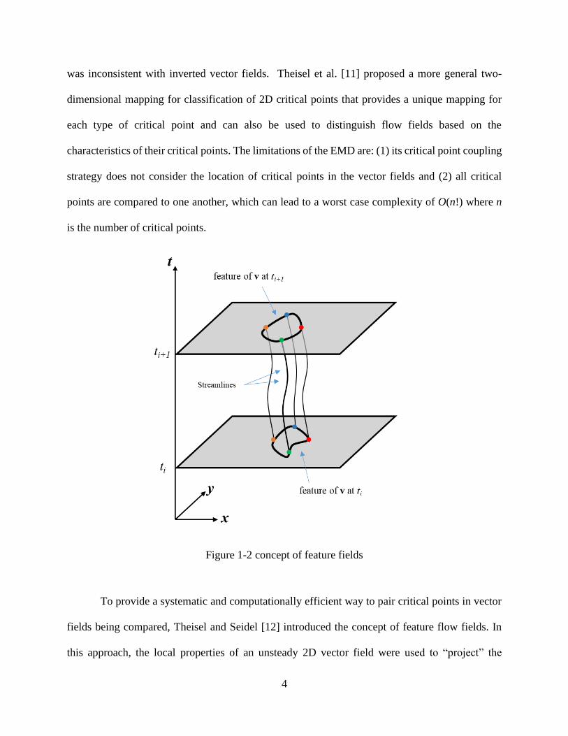
To provide a systematic and computationally efficient way to pair critical points in vector
fields being compared, Theisel and Seidel [12] introduced the concept of feature flow fields. In
this approach, the local properties of an unsteady 2D vector field were used to “project” the
Figure 1-2 concept of feature fields
Figure 1-2 concept of feature fields

5
expected location of critical points along constructed “streamlines” in time to match them with
their expected partners at a later time for comparison. The flow field defining these streamlines is
called the feature flow field and is constructed in a higher dimensional space to connected two
flow fields at different points in time. Figure 1-2 gives an illustration of the concept of feature flow
fields. The drawback of this approach is that it did not necessarily give meaningful results for flow
fields that are not very similar.
Batra et al. [14] gave an extension of the method introduced by Lavin et al. [8] by
considering not only the critical points but also the connectivity between them. By taking into
account the streamline connections of critical points (separatrices) in a given flow, they improved
the distance measurement of two different vector fields (i.e., made it more discriminating). The
critical points together with their separatrices formed an attributed relational graph and allowed
for flow field comparison based on the characteristics of the resulting graphs. This approach
seemed to improve the ability of the algorithm to identify different flow patterns.
More generally, a graph 𝐺 = (𝑉, 𝐸) in its basic form is made of vertices and edges. 𝑉 is
the set of vertices (also called nodes or points) and 𝐸 ⊂ 𝑉 × 𝑉 is the set of edges (also known as
arcs or lines) of graph G. The set 𝑉 can be considered the set of critical points for purposes of
characterizing flow fields based on these features. The edges 𝐸 can be constructed in many ways.
Proximity graphs [17] form edges based on some measure of the relative closeness of the points
they connect. As a special case, a Gabriel graph identifies edges between two points if there are
no other points in the circle formed with the identified edge as the diameter of the circle. Building
on this concept, Krueger et al. [19] developed a novel generalization of the Gabriel graph concept
in which weights are assigned to each edge in the complete graph based on how closely they match
the Gabriel criterion for edges. Then weighted Gabriel graphs based on critical points in flow fields

6
were compared in terms of weights of the graph edges to assess relative similarity of flow fields.
Using the idea of weighted Gabriel graphs makes the algorithm robust to the minor distortions in
the location of critical points and allows flow fields to be reliably categorized based on flow
topology.
1.2 Critical Point Detection
Clearly, there are many approaches to comparing flow fields using critical points and their
properties. This makes identifying and characterizing critical points an essential element of flow
field comparison using these methods.
Many of the current topological feature extraction algorithms are developed for
vortex/coherent structure detection and characterization of properties such as size, strength and
convection velocity [23]. They are based on streamline orientation, vorticity distribution and
velocity gradient tensor properties [24,25]. Algorithms based on these principles are extremely
sensitive to the quality of the vector field and are computationally intensive which limits their
application to experimental results [28].
Depardon et al. [28] developed a robust method for identifying and characterizing critical
points and applied it to fully analyze the near-wall topology of flow around a cube. Their algorithm
utilizes the concept of Poincare-Bendixon theorem from topological theory (also known as the
summation rule [29]) and has four steps, which will be described more in the next chapter. The
algorithm efficiently identifies all types of critical points, even from poor quality vector fields.
However, it is limited to 2D vector fields.
Mann and Rockwood [30] considered three-dimensional vector fields. They utilized the
Gauss-Bonnet theorem and an oct-tree algorithm to locate critical points. Their work is, however,
limited to the study of just the location of critical points and not their type. They also did not

7
consider identification of the sub-grid location of critical points, which may be important for
coarse-grid data.
1.3 Objectives
Considerable work is presented for identifying and characterizing critical points in 2D
vector fields, but less is available for 3D vector fields. Higher complexity levels in many 3D flows
makes the quantitative flow field comparison methods by identifying and characterizing critical
points potentially more valuable. However, the identification of the critical points should be done
in an efficient and robust way.
The objective of this work is developing an algorithm to identify critical points in 3D vector
fields that is:
I. Robust against noise
II. Efficient in poor quality and low-resolution vector fields
III. Not computationally intensive
The algorithm developed in this work is based on an extension of the method in Depardon et al.
[28] from 2D to 3D vector fields, integrating the Gauss-Bonnet theorem and vector field properties
to refine the location of critical points. The developed algorithm will be demonstrated on some
example vector fields.

8
CHAPTER 2
METHODOLOGY OF IDENTIFYING CRITICAL POINTS: ALGORITHM
In this chapter the algorithm used to find and identify critical points from vector fields is
described. First, the two-dimensional algorithm developed by Depardon et al. [34] is reviewed. In
the present work, the algorithm is extended to three-dimensional vector fields with appropriate
modifications. Table 1 shows the core functionality of the 2D procedure and the analogous 3D
components in the extended algorithm.
2D Systems 3D Systems
Step 1:
Coarse
Search
Orientation Test consisting of:
Orientation Histogram
Orientation Test consisting of:
Orientation Histogram
Step 2:
Confirmation
and location
refinement
Poincare-Bendixon Theorem Gauss-Bonnet Theorem
Step 3:
Subgrid
location
Γ (2.1), 𝑘 (2.2), Gradient of
flow field angle (2.3)
𝐹 (Gradient of sin and cos of
the flow field angle) (2.7)
Step 4:
Critical point
type
Eigenvalue problem Eigenvalue problem
The aim of the algorithm is to robustly identify the sub-grid locations and types of critical points
in the vector field for 3D vector fields.
2.1 Localization and Identification of Critical Points in 2D Vector Fields
In this section, the algorithm for identification of critical point in 2D vector fields
developed by Depardon et al. [34] is explained. Since the goal is to identify locations and types of
Table 2-1 Summary of 2D critical point algorithm and the 3D extension.
2D Systems 3D Systems
Step 1:
Course
Search
Orientation Test consisting
of:
Orientation Histogram
Orientation Test consisting
of:
Orientation Histogram
Step 2:
Confirmation
and location
refinement
Poincare-Bendixon Theorem Gauss-Bonnet Theorem
Step 3:
Subgrid
location
G, k, Grad F
Step 4:
Critical point
type
Eigenvalue problem Eigenvalue problem
Table 1 Summary of 2D critical point algorithm and the 3D extension.
Table 1 Summary of 2D critical point algorithm and the 3D extension.
2D Systems 3D Systems

9
critical points in vector fields, and a robust 2D algorithm exits, it will be reviewed first as it serves
as the basis for the 3D algorithm.
2.1.1 Topological Degree
The term topological degree refers to the Poincare-index of a critical point in a 2D vector
field. Given a curve immersed in a vector field, the Poincare-index is defined as the total rotation
of a base vector moving on the curve locally tangent to the vector field. For a closed curve in a
continuous 2D vector field the number of rotations of the based vector will always be an integer
since the start and end of the path will be identical [32]. Figure 2-1(a) shows an example of open
curve in a 2D vector field. Figure 2-1(b) shows the angle spanned when the origins of the vectors
at all locations along the path in Figure 2-1(a) are brought to the same point.
Figure 2- 1 Poincare-index calculation in 2D vector field
The topological degree of a critical point depends on the linear behavior of the vector field in the
neighborhood of the critical point. The Poincare index can characterize an isolated critical point.

10
The possible values for the index are +1 and -1 for a node and a saddle respectively. The
operational steps to evaluate the index for a candidate critical point are [33]:
1) Use a circle around the potential critical point as the path.
2) Place a unit vector on the circle locally tangent to the field vector at that point. This is the
base vector.
3) Move the base vector clockwise along the circle, around the candidate point such that the
vector is tangent to the local vector field at each point on the path.
4) Determine whether this unit vector has rotated by at least 2𝜋 radians about its base during
the translation of the vector’s base around the circle.
The following results from this procedure are possible:
I. The vector has rotated 2𝜋 radians in the clockwise direction about its base point, indicating
a node is enclosed within the circle.
II. The vector has rotated less than 2𝜋 radians about its base point and there is no (net) critical
point within the circle.
III. The vector has rotated 2𝜋 radians in the counterclockwise direction about its base point,
indicating a saddle is enclosed within the circle.
Figure 2-2 illustrates the three outcomes mentioned above with corresponding labels for each. It
is obvious from the figure in part (i), the base vector has rotated 2𝜋 radians in the clockwise
direction. Hence, the critical point is a node and the corresponding index is +1. In Figure 2-2 (iii)
the unit vector will rotate 2𝜋 radians in the counterclockwise direction. The counterclockwise
rotation results from the enclosed critical point being a saddle point with an index of -1.

11
It is worth noting that the property of critical points to rotate the vector field in their vicinity
provides a fast test to determine the potential location of critical points based on the overall
variability of the vector field orientation in the region near a point of interest. Such a test is utilized
as a first scan to find potential critical point zones in the algorithms presented below.
Figure 2- 2 mapping of vectors around different points with corresponding vector angle
histograms, i) a node (index +1) , ii) no-critical point (index zero), iii) a saddle (index -1)
2.1.2 The 2D Algorithm
In the sequential processing developed and used by Depardon et. al [28] to analyze critical
points in 2D vector fields, four main steps are utilized.
First, an orientation test is performed on the vector field, which is based on the observation
that the orientation of the vector field spans [0, 2π] in the neighborhood of a critical point as noted

12
in the discussion of the Poincare-index above. The goal of the orientation test is to identify regions
where a critical point is likely to be. This test consists of calculating the orientation histogram for
all field vectors within the region (neighborhood) surrounding a point of interest. The histogram
accumulates the local flow angle at each point within the selected region. For a region surrounding
a critical point, the percentage of non-empty bins approaches 100%. On the other hand, for a test
region containing no critical points, the histogram has peaks in some ranges within [0,2𝜋] and
empty bins elsewhere. Sample histograms are shown in Figure 2-2 for each case.
The non-empty bin percentage threshold and testing area size are two parameters that are
set by the investigator for this orientation test. The choice of threshold and testing area size depends
on the quality of the data. A test area size of around 5-7 grid points and a percentage of non-empty
bins of 75% was chosen by Depardon et al. [28] to identify regions that likely contain critical
points. This orientation test is then applied to regions surrounding every point in the vector field
and points with histograms passing the test are grouped together as regions which may contain one
or more critical points. It should be noted that any found potential critical point region may contain
no critical point (due to invalid or noisy data) or can hold one or more critical points. The results
of this step narrow the focus from the entire field domain to a few smaller regions of interest for
further processing. Figure 2-3 illustrates an example of flow orientation angles, 𝜃𝑃, that are used
to calculate the orientation histogram. Blue arrows represent velocity vectors in the flow field.
The next step in the algorithm is to iteratively apply the Poincaré-Bendixson theorem on
each potential critical point region identified by the orientation test in Step 1. The Poincaré-
Bendixson theorem is the following [28]: If 𝜃 is the angle between a vector function defined on a
plane and any fixed line, and ∆𝜃 is the accumulated change of 𝜃 while moving around a closed

13
loop on a plane, then Δ𝜃 2𝜋⁄ is equal to (number of nodal points within the loop) – (number of
saddle points within the loop). The value of Δ𝜃 2𝜋⁄ is called the Poincaré-Bendixson index.
Figure 2- 3 Flow orientation angles at four different points
The purpose of Step 2 is to further narrow the regions of interest in the field by eliminating
those that do not contain critical points and subdividing regions which contain more than one
critical point. Additionally, the Poincaré-Bendixson theorem permits an estimate of the true
locations of critical points, as well as discernment between nodal points and saddle points. Every
potential region identified in Step 1 is scanned by two rectangular loops with moving boundaries
each normal to the Cartesian directions. Each moving boundary divides the test region from Step
1 into two regions. For each region created by the moving boundary, the Poincaré-Bendixson index
is calculated. Prior to the moving boundary intersecting a critical point, if the Poincaré-Bendixson
indices are zero for both regions, there is no critical point or there is one pair of a saddle (−1) and
focus (+1) that cancel each other’s Poincaré-Bendixson index. As the boundary moves, if the

14
values of both Poincaré-Bendixson indices change, it has passed through a critical point, which
can be used to separate regions into sub-regions that contain only one critical point.
Figure 2- 4 illustration of θM at different points
Step 3 of the 2D algorithm determines the precise critical point location at the sub-grid
level. In the 2D case, this step is also useful for identifying the type of critical point. If the
Poincaré-Bendixson index is +1, then Γ1 and 𝐾1 are computed as follows:
Γ1(𝑃) = 1
𝑆 ∫ 𝑠𝑖𝑛(𝜃𝑀) 𝑑𝑆
𝑀∈𝑆
(2.1)
and
𝐾1(𝑃) = 1
𝑆∫ 𝑐𝑜𝑠(𝜃𝑀)𝑀∈𝑆
𝑑𝑆 (2.2)

15
where 𝑆 is a 2D area surrounding 𝑃, 𝑀 lies in 𝑆, and 𝜃𝑀 represents the angle between the velocity
vector at 𝑀 and the line 𝑃𝑀⃗⃗⃗⃗ ⃗⃗ . Equations (2.1), (2.2) are applied for all points 𝑃 within 𝑆. Figure 2-
4 shows four examples of 𝜃𝑀 calculated within 𝑆. Considering maximum values, if |Γ1| > |𝐾1|,
the type of critical point is a node, otherwise, it is a focus [36].
For a saddle point, which has Poincaré-Bendixson index equal to −1, |∇𝜃𝑀| for all points
𝑃 inside 𝑆 is used [28] instead of Γ1 and 𝐾1. The gradient, ∇𝜃𝑀, can be evaluated as:
∇𝜃𝑀 = ∇(sin 𝜃𝑀)
cos 𝜃𝑀 (2.3)
All three types of critical points occur at locations where the values of the corresponding functions
2.1-3 are extrema. Sub-grid localization of the critical points can then be obtained by interpolating
the result of the corresponding function to determine the location of the extremum, or by
computing the centroid of the corresponding function.
Step 4 in the 2D process is to identify the topology of each of the located critical points by
determining the eigenvalues of the velocity gradient tensor at the critical point location. Since
high-precision locations of critical points are found in Step 3, their eigenvalue and eigenvectors
are now readily obtainable. The eigenvectors determine the dynamically singular directions of the
critical points, providing topological information about the critical points [34]. The result is
numerical localization and identification of critical points in a 2D vector field.
2.2 Localization and Identification of Critical Points in 3D Vector Fields
The process of localizing and identifying critical points in three-dimensional vector fields
is structurally similar to the 2D vector field algorithm. Both strategies start with an orientation test
based on an orientation histogram as a rapid, course search to find regions that might contain

16
critical points (but in 3D the regions are volumes). These regions are then refined further by
computing the topology index for subdomains within the regions, where a topology index not equal
to zero indicates a critical point. In the following sections, the principles employed in 3D vector
fields are discussed. Subsequently, a generalization of the algorithm for extraction of precise
locations of critical points and their eigenvalues are developed and explained.
2.2.1 Gauss-Bonnet Theorem
The Gauss–Bonnet theorem is a functional theory for analyzing surfaces in differential
geometry. It connects geometry of the surface curvatures to their topology using the Euler
characteristic [37]. To assist in the discussion of Gauss-Bonnet theorem, it is helpful to define a
Gauss map. Let 𝑀 ⊂ 𝑅3 be a regular manifold. A manifold is a topological space that corresponds
to Euclidean space around any point. Then the Gauss map 𝛾:𝑀 → 𝑅3 derives its values at 𝑀 from
the values of the corresponding vector field as follows [30]: for a continuous vector field function,
𝑉:𝑀 → 𝑅3 with 𝒙 ∈ 𝑀,
𝛾(𝒙) ≡ 𝑉(𝒙)
|𝑉(𝒙)| (2.4)
If we consider a small sphere around a point 𝑐, and name the sphere, 𝐵(𝑐), the topological index
at 𝑐, 𝑖𝑛𝑑(𝑐), can be calculated by using the Gauss-Bonnet theorem [37]:
𝑖𝑛𝑑(𝑐) = ∫𝐾 𝑑 (𝛾(𝐵(𝑐)))
(𝑣𝑜𝑙𝑢𝑚𝑒 𝑜𝑓 𝐵(𝑐)) (2.5)
where 𝐾 is the Gaussian curvature of 𝛾(𝐵(𝑐)), equivalent to the product of the principle curvatures
of the surface. The normal curvature of a curve is the infinitesimal change of length at 𝑥 on a curve

17
compared to the change in 𝛾(𝑥) [37]. In 2D vector fields, the Gauss-Bonnet index is equivalent to
the count of vector field rotations or windings around 𝐵(𝑐).
Figure 2- 5 index number definition for a regular point (a) and a critical point (b)
The idea of the index or “winding” of a point c can be visualized as the surface covering
achieved by the vector field in the vicinity of a point c. Figure 2-5 shows a Gauss map for a region
devoid of critical points (a) as well as a map for a region containing a critical point (b). In the
figure the red arrows indicate the vectors in the field coincident with the surface of sphere 𝐵. The
selected Gauss map effectively coalesces these vectors to the center of the sphere, and projects
them onto the surface of the sphere to form a calculable area (blue). The index number, which
characterizes the flow, can be related to ratio of this covered area to the total surface of the sphere.
For a region devoid of critical points, the ratio is much less than one, and in the extreme case of
uniform flow the ratio is zero. For a volume containing a critical point, the ratio of the covered

18
surface to the total surface will be one. Note also that the range of orientations surrounding a
critical point is large, indicating an orientation test (as used in 2D) can be useful in identifying
points that are candidate critical points.
Taking the idea of the volume spanned by the Gauss map indicating the winding for the
vector field surrounding a point c, it is straightforward to rewrite the Gauss-Bonnet theorem in
terms of the underlying vector field surrounding c. To this end, a general formula employed by
Hestence [39] to compute the index number of a critical point for a 3D vector field, 𝑉, on manifold,
𝐵(𝑐), is given by
𝑖𝑛𝑑(𝑐) = 𝐷 ∫𝑉⋀ 𝑑𝑉
|𝑉|3
𝐵(𝑐)
(2.6)
Here the Geometric Algebra concept of a wedge product (see appendix) is used for computing the
volume between vectors in the numerator. The constant 𝐷 is a sphere normalization factor and
equals (6 × 4𝜋 3⁄ )−1. The extended differential 𝑑𝑉 is a bivector perpendicular to 𝑉, thus 𝑉 ∧ 𝑑𝑉
represents an infinitesimal volume element. Equation 2.6 results in a value between 0 and 1, with
1 indicating a critical point within 𝐵(𝑐).
2.3 The 3D Algorithm
The algorithm to locate and identify critical points in 3D vector fields consists of four steps
analogous to the 2D algorithm:
1. Globally scan the vector field with an orientation test to find regions that may contain
critical points.
2. Locally scan regions identified in Step 1 to refine the locations of critical points. Regions
devoid of critical points are eliminated from interest.

19
3. Calculate higher-precision sub-grid resolution locations of the critical points.
4. Identify the critical point type at each location.
As in the 2D algorithm, the result is a list of locations of critical points and their types which can
be used to quantitatively compare vector fields.
Step 1: Orientation Test: Orientation Histogram
The first scan of vector fields is to eliminate regions determined to not have critical points
and identify those that may have critical points for further processing. The process follows that
used for 2D vector fields given that the orientation of the vector field in regions near critical points
is variable as illustrated in Figure 2-6. Specifically, a volume of specified size near a point of
interested is selected and the histogram of vector directions in that volume is determined.
Figure 2- 6 iteration mechanism in step 1

20
In Figure 2-6, a critical point is shown on-grid in the horizontal direction and in between
nodes in the vertical direction. The scanning procedure, represented by the three squares/volumes
labeled 𝑖 = 1,2, and 3, is shown in just one direction but is also applied in the other two directions.
The green square (𝑖 = 3) in Figure 2-6, contains the critical point, so the point at the center of this
square will be identified as a candidate for a critical point. Continuing the scanning process
identifies several points around the critical point as candidates, which are then grouped together
as a region for further analysis.
As in 2D, the direction of the vectors is determined with respect to a reference direction,
such as a unit vector along the x-direction. This direction can be determined using the dot product
of the vectors with the reference direction and its value is in the range of [0, 2𝜋].
Another possible way to characterize the orientation of the flow field vectors is to consider
the azimuth and polar angles (or 𝜃 and 𝜑 in spherical coordinates). This method produces at 2D
histogram, which requires more vectors to fill the bins (obtained from a larger test volume), even
when a critical point is present. As a result, the results from considering one vector as reference
were simpler and faster to analyze.
A histogram of flow angle values is generated for each volume analyzed. Cubic volumes
surrounding points of interest were used, with the size selected by the user, but generally nine grid
points in each direction was found to be sufficient for this step. The histograms were constructed
with ten bins (each spanning 𝜋
5= 36°). As the number of empty bins increases, the probability of
having a critical point decreases. A threshold value of 50% of the bins being non-empty was found
experimentally to have good detection results at this stage in the algorithm. Figure 2-7 shows an
example histogram plot for a non-critical point (a) and a critical point (b). The empty bins in Figure

21
2-7 are characteristic of the absence of a critical point. Both the size of testing volume and non-
empty bin threshold are adjustable based on quality of the data. For example, a higher threshold
value can be selected for more noisy data. The testing volume size is specified by the number of
grid points included, so it automatically scales for coarser grids.
Figure 2- 7 Frequency distribution pattern for a non-CP (a) and a CP (b)
Generally, this test can be applied for volumes surrounding every point in the domain. Then
identified locations that passed the threshold test were grouped together into regions for further
processing in Step 2.
Step 2: Gauss-Bonnet Theorem for Refining Critical Point Detection
The orientation test is a fast computation to rapidly eliminate volumes that do not have
critical points. Due to the choice of threshold value, noise in the data, adjacency to a critical point,
etc., Step 1 may result in regions that are false positives for critical points or contain multiple
critical points. The Gauss-Bonnet theorem can be applied to robustly detect critical points in the

22
identified regions and divide them into subdomains containing only one critical point. However,
the computational cost is much greater.
To apply the Gauss-bonnet theorem to the regions identified in Step 1, the index for points
spanning the volume were computed using equation 2-6 applied to cubic volumes of 3 × 3 × 3 grid
points. This cube size is the smallest for which equation 2-6 can be applied so that the results are
as close to the local index for each point as is allowed by the data. The cubes are adjacent to each
other and have the maximum overlap to prevent missing any critical point on the boundaries
between cubes.
Figure 2-8 shows Step 2 in a 2D visualization of a 3D vector field with nodes at the corners
of squares. A critical point is shown on-grid in the horizontal direction and in between nodes in
the vertical direction. The scanning procedure is shown in just one direction but is applied in the
other two directions. The green square selected in Step 1 (figure 2-6) contains the critical point, so
the point at the center of this square will be identified as a candidate for a critical point. Continuing
the scanning process identifies several points around the critical point as candidates, which are
then grouped together as a region for further analysis. This region is shown in Figure 2-8 for
analysis with the Gauss-Bonnet theorem. The Gauss-Bonnet theorem may identify multiple
regions within the volume identified in Step 2 that have critical points. In the figure, the location
of the critical point is narrowed down to the volume selected in iteration 6 (𝑖 = 1 𝑡𝑜 6). To
precisely locate the critical point each 3 × 3 × 3 region is analyzed by Step 3.
Since the cubes used for computing the Gauss-Bonnet index of a point using equation 2-8
contain comparatively fewer data points than Step 1, a good threshold on the computed index for
identifying any cube as containing a critical point was experimentally found to be 0.50, even

23
though the Gauss-Bonnet formula has superior accuracy performance. The value of the index for
a non-critical point is typically less than 0.10, even for a vector field with a coarse grid.
Figure 2- 8 iteration mechanism in Step 2
Step 3: Sub-Grid Localization of Critical Points
The vector field direction in the neighborhood of a critical point changes dramatically, as
illustrated in Figure 2-2. The sub-grid location of the critical point can be found using this property.
This step is important for coarse grids, and data from experimental measurements. This can be
accomplished by calculating the gradient of the angles using a function 𝐹 [36], where for a 2D
vector field, the value of 𝐹 at a point 𝑃 is calculated as
𝐹(𝑃) = |∇sin(𝜃𝑃)| + |∇cos(𝜃𝑃)| (2.7)
Here 𝜃𝑃 is the angle between the velocity vector and a reference vector, as shown in Figure 2-4
(a). The value of 𝐹 is a maximum at the critical point location and decays to zero away from the
critical point, giving a convenient way to identify the location of the critical point if 𝐹 is computed
in the neighborhood of a critical point.
24
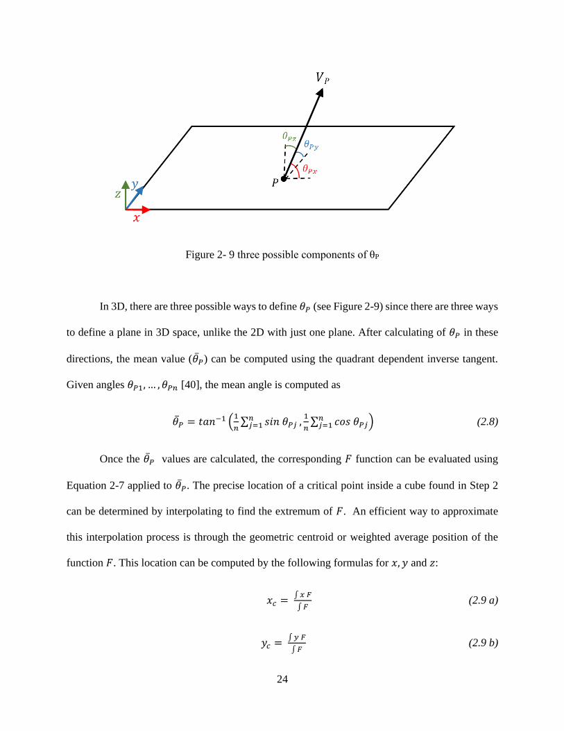
Figure 2- 9 three possible components of θP
In 3D, there are three possible ways to define 𝜃𝑃 (see Figure 2-9) since there are three ways
to define a plane in 3D space, unlike the 2D with just one plane. After calculating of 𝜃𝑃 in these
directions, the mean value (�̅�𝑃) can be computed using the quadrant dependent inverse tangent.
Given angles 𝜃𝑃1, … , 𝜃𝑃𝑛 [40], the mean angle is computed as
�̅�𝑃 = 𝑡𝑎𝑛−1 (1
𝑛∑ 𝑠𝑖𝑛 𝜃𝑃𝑗
𝑛𝑗=1 ,
1
𝑛∑ 𝑐𝑜𝑠 𝜃𝑃𝑗
𝑛𝑗=1 ) (2.8)
Once the �̅�𝑃 values are calculated, the corresponding 𝐹 function can be evaluated using
Equation 2-7 applied to �̅�𝑃. The precise location of a critical point inside a cube found in Step 2
can be determined by interpolating to find the extremum of 𝐹. An efficient way to approximate
this interpolation process is through the geometric centroid or weighted average position of the
function 𝐹. This location can be computed by the following formulas for 𝑥, 𝑦 and 𝑧:
𝑥𝑐 = ∫𝑥 𝐹
∫ 𝐹 (2.9 a)
𝑦𝑐 = ∫𝑦 𝐹
∫𝐹 (2.9 b)

25
𝑧𝑐 = ∫ 𝑧 𝐹
∫𝐹 (2.9 c)
The integration domain is the size of selected cubes from Step 2.
Step 4: Determining the Types of Critical Points
Given a Cartesian three dimensional fluid flow 𝑽, where 𝑽(𝑥, 𝑦, 𝑧) =
(𝑢(𝑥, 𝑦, 𝑧), 𝑣(𝑥, 𝑦, 𝑧), 𝑤(𝑥, 𝑦, 𝑧)), a first order description of the flow near an arbitrary point 𝒙0,
with background mean flow removed, can written as [41]:
[𝑢𝑣𝑤
] =
[ 𝜕𝑢
𝜕𝑥
𝜕𝑢
𝜕𝑦
𝜕𝑢
𝜕𝑧
𝜕𝑣
𝜕𝑥
𝜕𝑣
𝜕𝑦
𝜕𝑣
𝜕𝑧
𝜕𝑤
𝜕𝑥
𝜕𝑤
𝜕𝑦
𝜕𝑤
𝜕𝑧 ]
𝒙0
[
𝑥 − 𝑥0
𝑦 − 𝑦0
𝑧 − 𝑧0
] or 𝑉 = 𝐴(𝒙 − 𝒙0) (2.10)
where 𝐴 is the rate of deformation tensor at 𝒙0, and for a steady flow, the solution trajectories of
Equation 2-10 are equivalent to streamlines [41]. In 3D 𝐴 is the velocity gradient tensor. The
eigenvalues, 𝜆1, 𝜆2 and 𝜆3, of 𝐴 can be determined by solving the characteristic equation given by
𝜆3 + 𝑃𝜆2 + 𝑄𝜆 + 𝑅 = 0 (2.11)
where
𝑃 = − (𝜕𝑢
𝜕𝑥+
𝜕𝑣
𝜕𝑦+
𝜕𝑤
𝜕𝑧) (2.12)
𝑄 = |
𝜕𝑢
𝜕𝑥
𝜕𝑢
𝜕𝑦
𝜕𝑣
𝜕𝑥
𝜕𝑣
𝜕𝑦
| + |
𝜕𝑢
𝜕𝑥
𝜕𝑢
𝜕𝑧𝜕𝑤
𝜕𝑥
𝜕𝑤
𝜕𝑧
| + |
𝜕𝑣
𝜕𝑦
𝜕𝑣
𝜕𝑧
𝜕𝑤
𝜕𝑦
𝜕𝑤
𝜕𝑧
| (2.13)
and
𝑅 = − 𝑑𝑒𝑡[𝑨] (2.14)
26
Equation 2.14 can have (a) all real roots which are distinct, (b) all real roots where at least two
roots are equal, or (c) one real root and a conjugate pair of complex roots.
When 𝒙0 is a critical point, the eigenvalues of 𝐴 determine the nature of the critical point.
For example, if 𝑃 > 0, 0 < 𝑄 < 𝑃2 3⁄ , 0 < 𝑅 (𝑜𝑟 𝑅 < 0), the critical point is stable
Node/node/node. If 𝑃 > 0, 𝑃2 4⁄ < 𝑄 < 𝑃2 3⁄ , the critical point is a Node/node/star node A
complete list 12 possible critical point types is listed in Reference [41]. It should be noted that
center type critical points for 2D flows are degenerate cases in 3D as they are a cross-section of a
line of singularities in 3D. Such cases are outside the scope of this work.
Using the subgrid location of critical points determined in Step 3, the gradients of the
velocity field can be determined at the location of the critical point through various interpolation
methods in order to find 𝐴, and hence the eigenvalues, associated with the critical point. Here
Gaussian weighted interpolation is used to interpolate 𝐴 and find 𝐴𝑐 (𝐴 at the centroid), as
described in detail in the next chapter. The completion of Step 4 concludes the goals of the 3D
critical point localization and identification process, and a list of locations and types of critical
points in the vector field is produced. This information can subsequently be used to make
quantitative comparisons between fluid flows.

27
CHAPTER 3
IMPLEMENTATION AND RESULTS
In this chapter, implementation of the critical point identification algorithm is presented.
To validate the algorithm, some theoretical vector fields (e.g., from potential flow theory) were
utilized. Then, results of applying each step of the method are presented for the vector fields.
3.1 Implementation
Code was written in MATLAB 2018 to implement the critical point identification
algorithm. In the first step, the function angle_histogram is used to implement Step 1 of the
algorithm to identify critical points. The code for this function is given in Appendix 2.
The inputs needed for angle_histogram are the components of the velocity of the
vector field (𝑢, 𝑣, 𝑤), size of the test region, number of bins in the histogram and threshold of the
empty bins ratio. For the present results, a test region of eight grid points in each direction was
selected. The size of the interrogation volume can be set based on the grid size and noise level of
the data. Inside each interrogation volume, the angle between velocity vectors and a reference
vector is computed. The reference vector can be any constant vector as the purpose of this step is
just to know the orientation of the vectors inside the interrogation volume. Here, the reference
vector is chosen as 𝑟𝑒𝑓⃗⃗ ⃗⃗ ⃗⃗ = (1, 0, 0) to have faster computation time.
The number of bins in the histogram was set to be 10 for the tested flow fields. The
minimum recommended number of histogram bins is 5. The minimum number of bins was
determined from several runs of angle_histogram with different numbers of bins on regions

28
with critical points as well as on adjacent regions. The results showed that using 4 bins in the
histograms does not reliably produce results corresponding to the character of the tested region.
The interrogation volume is scanned over the entire data domain. At each location, the
frequency distribution (histogram plot) of angle values in the interrogation volume is evaluated.
The number of empty bins is evaluated and the center point of any interrogation volume that has
less than a specified threshold of empty bins is labeled as a potential critical point. The output of
the function is the indices of the potential critical points. For the data presented here, histograms
with ten bins at the range of [0, 2𝜋] were used and the empty-bin threshold was set 51%. The
threshold and number of bins are adjustable inputs to the function. The list of points output from
the angle_histogram function is then grouped into regions using the function
region_grouping. This function groups sets of adjacent points into continuous regions for
further processing.
The groups determined in Step 1 determine volumetric regions (subdomains of the
primary flow field) that are expected to contain critical points. The Gauss-Bonnet Theorem,
applied with the function called GB_index (given in Appendix 2), is used to determine
(approximately, i.e., to grid resolution) where in these regions the critical point(s) occur.
In GB_index the integral equation (2.6) is applied to the six faces of a rectangular
volume determined by three grid points in each coordinate direction and taking the velocity vectors
passing through each face of the volume on the associated regular grid 𝒑𝑖,𝑗,. Figure 3.1 shows the
vector sampling over a cube. After normalizing the velocity vectors, the trivectors 𝑅 and S
indicated in Figure 3.1 are computed as
𝑅𝑖,𝑗 = �̂�𝑖,𝑗 ∧ �̂�𝑖,𝑗+1 ∧ �̂�𝑖+1,𝑗 (3.1)

29
𝑆𝑖,𝑗 = �̂�𝑖+1,𝑗+1 ∧ �̂�𝑖+1,𝑗 ∧ �̂�𝑖,𝑗+1 (3.2)
for each grid square on each face.
Figure 3- 1 vector sampling over a cube (a) and positions of R and S on each face
Then, the surface integrals in equation 2-6 for each face are computed as sums all trivectors,
namely,
𝑅𝑓 = ∑𝑅𝑖,𝑗 and 𝑆𝑓 = ∑𝑆𝑖,𝑗 (3.3)
and the index of each volume is computed approximately as
𝑖𝑛𝑑(𝑐) ≈ ∑ 𝑅𝑓𝑖+ ∑ 𝑆𝑓𝑖
6𝑖=1
6𝑖=1
8𝜋 (3.4)
The value of 𝑖𝑛𝑑(𝑐) for a volume containing a critical point is close to one. This value decreases
for coarser grids. GB_index is applied on the entire region identified in Step 1. It identifies
locations where the index number is higher than the specified threshold and refines the critical

30
point locations for processing in Step 3. The output of the function is the indices corresponding to
any sub-volume of the input region that has been identified as potentially containing a critical
point.
To find the critical point location in the regions identified from GB_index as containing
critical points, the function 𝐹 (equation 2.7) is computed inside the selected volume, and the
centroid of this function is calculated using the rectangular rule to discretize equations (2.9).
With the subgrid location of the critical point known, the type of critical point is found
from the eigenvalues of the velocity gradient tensor at the location of the critical point, 𝑨𝒄
(equation 2.10). The value of 𝑨𝒄, is determined by interpolation of 𝑨 from the 8 nodes surrounding
the critical point, 𝐶, located at 𝐱𝑐 (Figure 3-2). Central differencing is used to calculate of the
velocity gradients in 𝑨 at the nodes and Gaussian weighted interpolation is used, namely
𝑨𝒄 = ∑ 𝑤𝑖𝐴𝑖
8𝑖=1
∑ 𝑤𝑖8𝑖=1
(3.5)
where
𝑤𝑖 = 𝑒|𝐱𝑖−𝐱𝑐|
2
𝜎2⁄ (3.6)
𝜎 represents standard deviation of the Gaussian function. The MATLAB function
interpolate_A implements this approach to determine the matrix 𝑨𝒄. The eigenvalues of
matrix 𝑨𝑐 uniquely determine the type of each critical point identified.

31
Figure 3- 2 Gaussian weighted interpolation to matrix A at the centroid
3.2 Vector fields for Algorithm validation
Vector fields generated from potential flow theory were used to check the accuracy of the
presented critical point extraction algorithm. Basic three-dimensional potential flow such as
source/sink and vortex are initially used to test the general correctness while developing first two
steps of the algorithm. After getting convincing results, more complicated vector fields were
generated and used to test the accuracy of the entire algorithm. Test vector fields of flow over a
sphere and a Ranking Body, and the vector field of the Lorenz Attractor were used for this purpose.
3.2.1 Three-dimensional potential flow over a sphere and Rankine Body
Three-dimensional potential flow over a sphere can be achieved by using superposition of
a 3D dipole (doublet) and uniform flow. More generally, a sink and source combination can be
used to approximate a doublet when close together, and provide more variety by varying the
distance between them. In this case the result is called flow around a Rankine body. The following
equations were derived for velocity values of a potential flow over a Rankine body:

32
𝑈 = (𝑈∞ cos 𝜃) − (Λ (𝑋 − ℓ cos(𝜃))
((𝑋 − ℓ cos(𝜃))2 + (𝑌 − ℓ sin(𝜃))2 + 𝑍2)32
) + (Λ (𝑋 + ℓ cos(𝜃))
((𝑋 + ℓ cos(𝜃))2 + (𝑌 + ℓ sin(𝜃))2 + 𝑍2)32
)
(3.7a)
𝑉 = (𝑈∞ sin 𝜃 ) − (Λ (𝑌 − ℓ sin(𝜃))
((𝑌 − ℓ sin(𝜃))2 + (𝑋 − ℓ cos(𝜃))2 + 𝑍2)32
) + (Λ (𝑌 + ℓ sin(𝜃))
((𝑌 + ℓ sin(𝜃))2 + (𝑋 + ℓ cos(𝜃))2 + 𝑍2)32
)
(3.7b)
𝑊 = −(Λ 𝑍
( (𝑋 − ℓ cos(𝜃))2 + (𝑌 − ℓ sin(𝜃))2 + 𝑍2)32
) + (Λ𝑍
((𝑋 + ℓ cos(𝜃))2 + (𝑌 + ℓ sin(𝜃))2 + 𝑍2)32
)
(3.7c)
where 𝛬 is a scaling constant called the sink/source strength, 𝜃 represents the horizontal angle of
uniform flow in the 𝑥𝑦 plane and ℓ is the distance between the sink and the source. Flow over a
nearly spherical surface is achievable by using very small values of ℓ.
Figure 3- 3 entire 3D potential flow over a sphere (a), cross section of the same flow field with
shown critical points by red dots (b)

33
To generate a discrete flow field, a built-in MATLAB function, meshgrid, was used to
create a 3D grid at specified coordinates. Then equations 3-7 were evaluated at the grid points.
Figure 3.3 (a) illustrates the entire 3D potential flow over a sphere and in Figure 3.3 (b) the cross
section of the same flow field is shown. Streamlines are used instead of vectors to better represent
the flow fields. There are two Node/Saddle/Saddle (NSS) critical points at the front and back of
the sphere (shown in Figure 3.3 (b) by red dots). The grid spacing is 0.25 which means 4 grid
points in one unit distance. The radius of the sphere is 4 which includes 16 grid points in each
coordinate direction.
Figure 3- 4 Rankine body flow with relatively small critical point spacing (red dots represent
critical points)

34
Rankine body flow field can be used to create a case that has two critical points very close to each
other. In such cases, the output of Step 1 of the algorithm can be just one region including two
critical points. Then in Step 2, the Gauss-Bonnet theorem should recognize the two critical points
in this region. Figure 3-4 shows the cross section of a Rankine body flow field in the 𝑥𝑦 plane.
This flow is considered to check the robustness of the algorithm at Step 2. The grid size in this
figure is 0.25 and the separation between the critical points in terms of grid units is about 5.
3.2.2 Lorenz Attractor
The Lorenz Attractor is an attractor for a system state that emerges from a simplified
system of equations explaining the flow of fluid with uniform depth in the presence of temperature
difference, gravity (buoyancy), thermal diffusivity and viscosity [42]. In the early 1960s, Lorenz
accidentally discovered the chaotic behavior of this system when he found periodic solutions for
Rayleigh numbers larger than a critical value. His equations, obtained for a simplified convective
system [42], can be represented as
�̇� = 𝜎(𝑌 − 𝑋) (3.8a)
�̇� = −𝑋𝑍 + 𝑟 𝑋 − 𝑌 (3.8b)
�̇� = 𝑋𝑌 − 𝑏 𝑍 (3.8c)
Now known as Lorenz equations, 𝜎 represents the Prandtl number, 𝑟 is the ratio of Rayleigh
number to the critical Rayleigh number, and 𝑏 is a geometric factor [43]. Lorenz took 𝑏 = 8 3⁄
and 𝜎 = 10. Therefore, the vector field for the state variables can be written as
�⃗� = (10(𝑦 − 𝑥), 28𝑥 − 𝑦 − 𝑥𝑧, 𝑥𝑦 − 8𝑧
3 ) (3.9)

35
This vector field has three critical points. The critical point at (0, 0, 0) is a NSS point and
corresponds to no convection. The critical points at (6√2, 6√2, 27) and (−6√2,− 6√2, 27) are
spiral saddle points and correspond to steady convection. These points are shown in Figure 3.5 as
red dots on a Lorenz attractor state flow domain.
Figure 3- 5 Lorentz attractor state flow domain with shown critical points (red dots)

36
3.3 Results and discussion
The results of each explained step of the critical identification algorithm in 3D vector fields are
presented and discussed in this section.
Figure 3- 6 histogram plots from implementation of step 1 on three different points b (critical
point) and a, c (non-critical point)
Figure 3-6 shows the implementation first step of the critical point identification algorithm
(angle orientation test) on half of the domain for flow over a sphere. Only the xy cross section of
the flow through the middle of the sphere is shown for clarity. The three histogram plots on the
right side are results of the angle orientation test within the interrogation volumes holding a critical
point (b) and also volumes adjacent to the same critical point (a, c). As discussed in Chapter 2, a

37
high number of non-empty bins on the histogram plots is used to identify a region as potentially
holding a critical point. Clearly interrogation volume (b) passes the test as all histogram bins are
full.
Figure 3- 7 outcome of flow orientation test (step 1) on the entire flow
Figure 3-7 provides the outcome of scanning of the entire flow domain presented in Figure
3-6. Each red dot on the plot represents the center of an interrogation volume identified as
potentially having a critical point. The axis values in the 𝑥, 𝑦 and 𝑧 directions are the corresponding
indices in the domain grid. Since there is overlap between interrogation volumes at each step of
the scanning process, a large number of locations can be identified as potential critical points. At
this point the algorithm simply outputs the minimum and maximum index values in all three

38
directions. The minimum and maximum index values in Figure 3-7 are (2,8) in 𝑥 direction and
(4,10) in 𝑦 and 𝑧 directions.
Figure 3- 8 flow orientation scan (a), Gauss-Bonnet index evaluation (b) on the flow field shown
in Figure 3-4
In Step 2 of the algorithm, the Gauss-Bonnet index evaluation, is applied only to the regions
found in the first step. It is designed to confirm that critical point(s) is (are) present, down-size the
identified regions to points nearest to the critical point, and split regions if there is more than one
critical point present. Figure 3-8 shows the implementation of flow orientation scan (a) and Gauss-
Bonnet index evaluation (b) for the entire flow field presented in Figure 3-4. As shown in Figure
3-8, calculation of the Gauss-Bonnet index (b) can be more robust and precise not only in detecting
location of critical points but also in the number critical points. However, this method needs about
10 times more time compared to the flow orientation scan (a). For this reason, the Gauss-Bonnet
index evaluation is applied just on the regions that were identified from flow orientation scan (Step
1).

39
Figure 3-9 shows the isosurface of the 𝐹 function (equation 2-7) and location of geometric
centroid of 𝐹 for the NSS point (b) and one of spiral node points (a) in the Lorenz Attractor field
(Figure 3-5). The calculated centroid location from the algorithm (Step 3) is shown as a red dot for
each point. The grid spacing for the data shown in Figure 3-9 is 0.25. Comparing the computed
critical points locations with the critical point locations from theory, shows that there is an
acceptable level of accuracy (one fifth of flow field grid sizing in each direction) in finding location
of critical points to subgrid accuracy.
Figure 3- 9 Corresponding isosurface plots and eigen values of spiral saddle point (a) and NSS
point (b) of a Lorentz Attractor flow field

40
With the locations of the critical points known the eigenvalues of the flow field were
calculated in Step 4 to identify the type of critical points. For this example, the eigenvalues
calculated for the NSS point (figure 3-9 b) were −22.84, 11.84 and −2.67. Also, the eigenvalues
for the spiral saddle point (figure 3-9 a) were −13.82 and 0.078 ± 10.16 𝑖. Both cases give the
same type of critical point expected from theory.

41
CHAPTER 4
CONCLUSION
Classification of vector fields containing vortical patterns such as flow around blocks and
oscillating cylinders and animal locomotion relates important observations about their
hydrodynamic behaviors (drag force) and propulsion efficiency, respectively. Traditionally flow
field classification is achieved qualitatively based on flow field images which is a subjective
method that becomes more difficult to apply as the vector fields are more complex. Characterizing
vector fields based on their graphical structure determined from the location of extracted features
(critical points) makes it possible to compare different flow fields quantitatively. This approach
provides a practical way to handle the complexity and size of modern flow simulations and
experimental data sets.
To facilitate quantitative classification of complex, 3D flow fields, a new algorithm is
presented to identify and characterize critical points in 3D vector fields. The algorithm is a 3D
extension of the approach introduced by Depardon et al. [28] focusing on 2D data. The present
algorithm has 4 steps to locate and specify the type of critical points. In the first step, the vector
field flow orientation is scanned with respect to a reference direction to roughly locate the regions
potentially containing critical points. The main reason to embed step 1 in the algorithm is to reduce
computation time. In step 2, the algorithm surveys regions identified from the previous step in
terms of the Gauss-Bonnet (GB) index to locate critical points with higher accuracy. Step 3 of the
algorithm is to identify critical point locations to sub-grid accuracy. This step makes the algorithm
efficient for low resolution vector fields. Finally in step 4, eigenvalues of the identified critical
points are calculated in order to characterize type of each critical point.

42
Accuracy and efficiency of the algorithm were tested on test flow fields including potential flows
and the Lorentz attractor with known locations of critical points as well as their types. Results
show that the presented algorithm is able to identify and classify critical points in 3D vectors fields
accurately enough by comparing with the exact theoretical. For future work, the algorithm needs
to be applied to vector fields resulted from numerical simulation and experimental data from
volumetric 3D flow field measurements such as defocusing digital particle tracking velocimetry
(DDPTV, see [44], [45], and [46] for additional information about this technique and related
methods).

43
REFERENCES
1. Depardon, S., Lasserre, J. J., Brizzi, L. E., & Borée, J. (2007). Automated topology
classification method for instantaneous velocity fields. Experiments in Fluids, 42(5),
697-710.
2. Becker, S., Lienhart, H., & Durst, F. (2002). Flow around three-dimensional obstacles
in boundary layers. Journal of Wind Engineering and Industrial Aerodynamics, 90(4-
5), 265-279.
3. Rockwell, D. (2000). Imaging of unsteady separated flows: global interpretation with
particle image velocimetry. Experiments in fluids, 29(1), S255-S273.
4. Bonnet, J. P., Delville, J., Glauser, M. N., Antonia, R. A., Bisset, D. K., Cole, D. R., ...
& Kevlahan, N. K. R. (1998). Collaborative testing of eddy structure identification
methods in free turbulent shear flows. Experiments in Fluids, 25(3), 197-225.
5. Dubuisson, M. P., & Jain, A. K. (1994). A modified Hausdorff distance for object
matching. In Proceedings of 12th international conference on pattern recognition (Vol.
1, pp. 566-568). IEEE.
6. Helman, J., & Hesselink, L. (1989). Representation and display of vector field topology
in fluid flow data sets. Computer, (8), 27-36.
7. Eiter, T., & Mannila, H. (1997). Distance measures for point sets and their computation.
Acta Informatica, 34(2), 109-133.
8. Lavin, Y., Batra, R., & Hesselink, L. (1998). Feature comparisons of vector fields using
earth mover's distance. In Proceedings Visualization'98 (Cat. No. 98CB36276) (pp.
103-109). IEEE.
9. Y. Rubner, C. Tomasi, and L. J. Guibas, “A metric for distributions with applications
to image databases,” in Proc. IEEE Internations Conferences on Computer Vision,
1998.
10. Lavin, Y., Batra, R., & Hesselink, L. (1998). Feature comparisons of vector fields using
earth mover's distance. In Proceedings Visualization'98 (Cat. No. 98CB36276) (pp.
103-109). IEEE.
11. Theisel, H., & Weinkauf, T. (2002). Vector field metrics based on distance measures
of first order critical points.
12. H. Theisel and H.-P. Seidel. Feature Flow Fields. In Proceedings of the
JointEurographics - IEEE TCVG Symposium on Visualization (VisSym 03),
pages141–148, 2003.

44
13. Perry, A. E., & Fairlie, B. D. (1975). Critical points in flow patterns. In Advances in
geophysics (Vol. 18, pp. 299-315). Elsevier.
14. R. Batra, K. Kling, and L. Hesselink. Topology based vector field comparison using
graph methods. In A. Varshney, C.M. Wittenbrink, and H. Hagen, editors, Proc. IEEE
Visualization ’98, Late Breaking Hot Topics, pages 25–28, 1999.
15. Batra, R., Kling, K., & Hesselink, L. (2000, February). Topology-based methods for
quantitative comparisons of vector fields. In Visual Data Exploration and Analysis
VII (Vol. 3960, pp. 268-279). International Society for Optics and Photonics.
16. Jaromczyk, J. W., & Toussaint, G. T. (1992). Relative neighborhood graphs and their
relatives. Proceedings of the IEEE, 80(9), 1502-1517.
17. Toussaint, G. T. (1980). The relative neighborhood graph of a finite planar set. Pattern
recognition, 12(4), 261-268.
18. Gabriel, K. R., & Sokal, R. R. (1969). A new statistical approach to geographic
variation analysis. Systematic zoology, 18(3), 259-278.
19. Krueger, P. S., Hahsler, M., Olinick, E. V., Williams, S. H., & Zharfa, M. (2019).
Quantitative classification of vortical flows based on topological features using graph
matching. Proceedings of the Royal Society A, 475(2228), 20180897.
20. G. Scheuermann, H. Hagen, H. Kruger, M. Menzel, and A. Rockwood. Visualization
of Higher Order Singularities in Vector Fields. In Proceedings IEEE Visualization ’97,
pages 67–74, October 1997.
21. G. Scheuermann, H. Kruger, M. Menzel, and A. P. Rockwood. Visualizing Nonlinear
Vector Field Topology. IEEE Transactions on Visualization and Computer Graphics,
4(2):109–116, April/June 1998.
22. Garth, C., Tricoche, X., & Scheuermann, G. (2004). Tracking of vector field
singularities in unstructured 3D time-dependent datasets. In Proceedings of the
conference on Visualization'04 (pp. 329-336). IEEE Computer Society.
23. Vollmers, H. (2001). Detection of vortices and quantitative evaluation of their main
parameters from experimental velocity data. Measurement Science and
Technology, 12(8), 1199.
24. Jeong, J., & Hussain, F. (1995). On the identification of a vortex. Journal of fluid
mechanics, 285, 69-94.

45
25. Helman, J. L., & Hesselink, L. (1990). Surface representations of two-and three-
dimensional fluid flow topology. In Proceedings of the 1st conference on
Visualization'90 (pp. 6-13). IEEE Computer Society Press.
26. Perry, A. E., & Chong, M. S. (1994). Topology of flow patterns in vortex motions and
turbulence. Applied Scientific Research, 53(3-4), 357-374.
27. Ford, R. M. (1997). Critical point detection in fluid flow images using dynamical
system properties. Pattern Recognition, 30(12), 1991-2000.
28. Depardon, S., Lasserre, J. J., Brizzi, L. E., & Borée, J. (2006). Instantaneous skin-
friction pattern analysis using automated critical point detection on near-wall PIV
data. Measurement Science and Technology, 17(7), 1659.
29. Foss, J. F. (2004). Surface selections and topological constraint evaluations for flow
field analyses. Experiments in fluids, 37(6), 883-898.
30. Mann, S., & Rockwood, A. (2002). Computing singularities of 3D vector fields with
geometric algebra. In Proceedings of the conference on Visualization'02 (pp. 283-290).
IEEE Computer Society.
31. Lay, D. C. (2005). Linear Algebra and its Applications, 3rd updated Edition.
32. Greene, J. M. (1992). Locating three-dimensional roots by a bisection method. Journal
of Computational Physics, 98(2), 194-198.
33. Foss, J. F. (2004). Surface selections and topological constraint evaluations for flow
field analyses. Experiments in fluids, 37(6), 883-898.
34. Graftieaux, L., Michard, M., & Grosjean, N. (2001). Combining PIV, POD and vortex
identification algorithms for the study of unsteady turbulent swirling
flows. Measurement Science and technology, 12(9), 1422.
35. Michard M, Graftieaux L, Lollini L and Grosjean N 1997 Proc. 11th Conf. on Turbulent
Shear Flows (Grenoble)
36. Cormier, N., Cormier, G., Poitras, G., & Brizzi, L. É. (2012). Automated critical point
identification for PIV data using multimodal particle swarm optimization. International
Journal for Numerical Methods in Fluids, 70(7), 923-938.
37. D. Gottlieb. All the way with Gauss-Bonnet and the sociology of mathematics. Amer.
Math. Monthly, 103(6):457–469, 1996.
38. Franchini, Silvia & Vassallo, Giorgio & Sorbello, F.. (2010). A brief introduction to
Clifford algebra.

46
39. Hestenes, D., & Sobczyk, G. (2012). Clifford algebra to geometric calculus: a unified
language for mathematics and physics (Vol. 5). Springer Science & Business Media.
40. Bishop, C. M. (2006). Pattern recognition and machine learning. Springer Science+
Business Media.
41. Chong, M. S., Perry, A. E., & Cantwell, B. J. (1990). A general classification of three‐
dimensional flow fields. Physics of Fluids A: Fluid Dynamics, 2(5), 765-777.
42. Weisstein, Eric W. "Lorenz Attractor." From MathWorld--A Wolfram Web Resource.
http://mathworld.wolfram.com/LorenzAttractor.html
43. Moffatt, Henry Keith, and Arkady Tsinober, eds. Topological Fluid Mechanics:
Proceedings of the IUTAM Symposium, Cambridge, UK, 13-18 August, 1989.
Cambridge University Press, 1990.
44. Pereira, Francisco, and Morteza Gharib. "Defocusing digital particle image velocimetry
and the three-dimensional characterization of two-phase flows." Measurement Science
and Technology 13.5 (2002): 683.
45. Couch, Lauren D., and Paul S. Krueger. "Experimental investigation of vortex rings
impinging on inclined surfaces." Experiments in fluids 51.4 (2011): 1123-1138.
46. Pereira, F., Stüer, H., Graff, E. C., & Gharib, M. (2006). Two-frame 3D particle
tracking. Measurement science and technology, 17(7), 1680.

47
APPENDIX 1
Geometric Algebra, also known as Clifford Algebra, is a mathematical tool to model and
transform geometric objects directly into algebraic expressions [38]. Geometric objects such as
points, lines and planes can be transformed into basic computational elements by utilizing
Geometric Algebra.
Geometric Algebra introduces a vector-vector outer product operator known as the wedge
product. The wedge product of two vectors results in a surface spanned by the two vectors and its
associated orientation (analogous to the cross-product of two vectors). Figure 1-A (b) illustrates
the result of the wedge products of two of the three vectors.. The ⋀ symbol, pronounced “wedge,”
is used to denote an outer product (𝒑 ⋀ 𝒒), also called a bivector or oriented area. Compare this
to a vector which is an oriented length.
Figure 1-A vector (a), bivector (b) and trivector (c)
Figure 2-6 vector, bivector and trivector

48
In the case of three vectors 𝒑 , 𝒒 and 𝒓, the result of (𝒑 ∧ 𝒒) ∧ 𝒓 is a three-dimensional
subspace. The bivector resulting from the first operation is extended by a third vector, creating an
oriented volume element. This oriented volume element is referred to as a trivector and is shown
in Figure 1-A (c).

49
APPENDIX 2
function[location_bar_index,groups] =
angle_histogram(U,V,W,block_size,n_bins,tresh_hld)
% applies step 1 of the algorithm to find potential CP regions
%
% M. Zharfa
% Southern Methodist University
% December, 2019
for i = 1:size(U,1)
for j = 1:size(V,2)
for k = 1:size(W,3)
U_norm(i,j,k) = U(i,j,k) ./ ( U(i,j,k).^2 + V(i,j,k).^2 +
W(i,j,k).^2 ).^(0.5);
V_norm(i,j,k) = V(i,j,k) ./ ( U(i,j,k).^2 + V(i,j,k).^2 +
W(i,j,k).^2 ).^(0.5);
W_norm(i,j,k) = W(i,j,k) ./ ( U(i,j,k).^2 + V(i,j,k).^2 +
W(i,j,k).^2 ).^(0.5);
end
end
end
grid_x = (max(X(:))-min(X(:)))/(size(X,1)-1);
grid_y = (max(Y(:))-min(Y(:)))/(size(Y,1)-1);
grid_z = (max(Z(:))-min(Z(:)))/(size(Z,1)-1);
m_x = block_size*grid_x ;
m_y = block_size*grid_y ;
m_z = block_size*grid_z ;
m = m_x;
i = 1:m_x:size(U,1)-m_x ;
j = 1:m_y:size(V,2)-m_y ;
k = 1:m_z:size(W,3)-m_z;
for a = 1:length(i)
for b = 1:length(j)
for c = 1:length(k)
U_norm_elm =
U_norm(i(a):i(a)+m_x,j(b):j(b)+m_y,k(c):k(c)+m_z);
angle = acosd(U_norm_elm) ;
AA = reshape(angle,1,[]);
bin_width = 360/n_bins;
N1 = histcounts(AA,0:bin_width:360);
bar_index(a,b,c) = 100*(sum(~N1(:))/length(N1));
end
end
end

50
[yy,xx,zz] = ind2sub(size(bar_index),find(bar_index <
tresh_hld));
location_bar_index = [xx,yy,zz];
groups = region_grouping(location_bar_index);
location_index(:,1) = (m_x * location_bar_index(:,1)) ;
location_index(:,2) = (m_y * location_bar_index(:,2)) ;
location_index(:,3) = (m_z * location_bar_index(:,3)) ;
end
%---------------------------------------------------------------
------
function [index] =
GB_index(i_1,i_2,j_1,j_2,k_1,k_2,U_norm,V_norm,W_norm)
%Function GB_index -- calculates Gauss Bonnet index using the
paper:
%
%
https://dl.acm.org/doi/pdf/10.5555/602099.602143?download=true
%
% where
% inputs:
% i_1,i_2,j_1,j_2,k_1,k_2:
% Specify the borders of the cube (test region)
% U_norm,V_norm,W_norm:
% normalized vetor field components
% Subroutines called: wedge
%
% M. Zharfa
% Southern Methodist University
% December, 2019
U_norm_2d_fr = U_norm(j_1:j_2,i_2,k_1:k_2);
V_norm_2d_fr = V_norm(j_1:j_2,i_2,k_1:k_2);
W_norm_2d_fr = W_norm(j_1:j_2,i_2,k_1:k_2);
BU_fr =
reshape(U_norm_2d_fr,size(U_norm_2d_fr,1),size(U_norm_2d_fr,3));
BV_fr =
reshape(V_norm_2d_fr,size(V_norm_2d_fr,1),size(V_norm_2d_fr,3));
BW_fr =
reshape(W_norm_2d_fr,size(W_norm_2d_fr,1),size(W_norm_2d_fr,3));
[R_fr_2,S_fr_2] =
wedge(flipud(BU_fr),flipud(BV_fr),flipud(BW_fr));
U_norm_2d_bk = U_norm(j_1:j_2,i_1,k_1:k_2);
V_norm_2d_bk = V_norm(j_1:j_2,i_1,k_1:k_2);
W_norm_2d_bk = W_norm(j_1:j_2,i_1,k_1:k_2);
BU_bk =
reshape(U_norm_2d_bk,size(U_norm_2d_bk,1),size(U_norm_2d_bk,3));
BV_bk =
reshape(V_norm_2d_bk,size(V_norm_2d_bk,1),size(V_norm_2d_bk,3));

51
BW_bk =
reshape(W_norm_2d_bk,size(W_norm_2d_bk,1),size(W_norm_2d_bk,3));
[R_bk_2,S_bk_2] = wedge(BU_bk,BV_bk,BW_bk);
U_norm_2d_tp = U_norm(j_2,i_1:i_2,k_1:k_2);
V_norm_2d_tp = V_norm(j_2,i_1:i_2,k_1:k_2);
W_norm_2d_tp = W_norm(j_2,i_1:i_2,k_1:k_2);
BU_tp =
reshape(U_norm_2d_tp,size(U_norm_2d_tp,2),size(U_norm_2d_tp,3));
BV_tp =
reshape(V_norm_2d_tp,size(V_norm_2d_tp,2),size(V_norm_2d_tp,3));
BW_tp =
reshape(W_norm_2d_tp,size(W_norm_2d_tp,2),size(W_norm_2d_tp,3));
[R_tp_2,S_tp_2] = wedge(BU_tp,BV_tp,BW_tp);
U_norm_2d_bt = U_norm(j_1,i_1:i_2,k_1:k_2);
V_norm_2d_bt = V_norm(j_1,i_1:i_2,k_1:k_2);
W_norm_2d_bt = W_norm(j_1,i_1:i_2,k_1:k_2);
BU_bt =
reshape(U_norm_2d_bt,size(U_norm_2d_bt,2),size(U_norm_2d_bt,3));
BV_bt =
reshape(V_norm_2d_bt,size(V_norm_2d_bt,2),size(V_norm_2d_bt,3));
BW_bt =
reshape(W_norm_2d_bt,size(W_norm_2d_bt,2),size(W_norm_2d_bt,3));
[R_bt_2,S_bt_2] =
wedge(flipud(BU_bt),flipud(BV_bt),flipud(BW_bt));
U_norm_2d_rt = U_norm(j_1:j_2,i_1:i_2,k_1);
V_norm_2d_rt = V_norm(j_1:j_2,i_1:i_2,k_1);
W_norm_2d_rt = W_norm(j_1:j_2,i_1:i_2,k_1);
BU_rt = U_norm_2d_rt;
BV_rt = V_norm_2d_rt;
BW_rt = W_norm_2d_rt;
[R_rt_2,S_rt_2] =
wedge(flipud(BU_rt),flipud(BV_rt),flipud(BW_rt));
U_norm_2d_lt = U_norm(j_1:j_2,i_1:i_2,k_2);
V_norm_2d_lt = V_norm(j_1:j_2,i_1:i_2,k_2);
W_norm_2d_lt = W_norm(j_1:j_2,i_1:i_2,k_2);
BU_lt = U_norm_2d_lt;
BV_lt = V_norm_2d_lt;
BW_lt = W_norm_2d_lt;
[R_lt_2,S_lt_2] = wedge(BU_lt,BV_lt,BW_lt);
AAAA = [sum(R_fr_2(:)) sum(S_fr_2(:)); sum(R_bk_2(:))
sum(S_bk_2(:)); sum(R_tp_2(:)) sum(S_tp_2(:)); sum(R_bt_2(:))
sum(S_bt_2(:)); sum(R_lt_2(:)) sum(S_lt_2(:)); sum(R_rt_2(:))
sum(S_rt_2(:))];
index = (sum(AAAA(:))/(6*4*pi/3),7);
end
%---------------------------------------------------------------
------

52
%Function wedge -- R,S(more information in the link below):
%
%
https://dl.acm.org/doi/pdf/10.5555/602099.602143?download=true
:
% equation (3) and implementation (part 5)
%
% where
% inputs:
% BU,BV,BW:
% created in GB_index function ( selected faces at front,
bottom, back, top, right and left)
% Subroutines called: NA
%
% M. Zharfa
% Southern Methodist University
% December, 2019
function [R,S] = wedge(BU,BV,BW)
for i = 1:size(BU,1)-1
for j = 1:size(BU,2)-1
R(i,j) = det([BU(i,j) BV(i,j) BW(i,j); BU(i,j+1) BV(i,j+1)
BW(i,j+1); BU(i+1,j) BV(i+1,j) BW(i+1,j)]);
S(i,j) = det([BU(i+1,j+1) BV(i+1,j+1) BW(i+1,j+1); BU(i+1,j)
BV(i+1,j) BW(i+1,j); BU(i,j+1) BV(i,j+1) BW(i,j+1)]);
end
end
end
%---------------------------------------------------------------
function[A_c]=
interpolate_A(X,Y,Z,U,V,W,xc_index,yc_index,zc_index,sigma)
% Matrix A at centroid calculator (used in step 4)
% U,V,W,X,Y,Z,xc,yc,zc are inputs
% used subfunctions: WW and dqdx, dqdy, dqdz
% output: e = (e1,e2,e3) (eigen values for the field at F
function centroid (xc,yc,zc)
% M. Zharfa
% December 2019
x1 = floor(xc_index);
x2 = x1+1;
y1 = floor(yc_index);
y2 = y1+1;
z1 = floor(zc_index);
z2 = z1+1;
p1 = [unique(X(:,x1,:)),unique(Y(y1,:,:)),unique(Z(:,:,z1))];

53
p2 = [unique(X(:,x2,:)),unique(Y(y1,:,:)),unique(Z(:,:,z1))];
p3 = [unique(X(:,x2,:)),unique(Y(y2,:,:)),unique(Z(:,:,z1))];
p4 = [unique(X(:,x1,:)),unique(Y(y2,:,:)),unique(Z(:,:,z1))];
p5 = [unique(X(:,x1,:)),unique(Y(y1,:,:)),unique(Z(:,:,z2))];
p6 = [unique(X(:,x2,:)),unique(Y(y1,:,:)),unique(Z(:,:,z2))];
p7 = [unique(X(:,x2,:)),unique(Y(y2,:,:)),unique(Z(:,:,z2))];
p8 = [unique(X(:,x1,:)),unique(Y(y2,:,:)),unique(Z(:,:,z2))];
A1 = [dqdx(U,X,y1,x1,z1) dqdy(U,Y,y1,x1,z1) dqdz(U,Z,y1,x1,z1);
dqdx(V,X,y1,x1,z1) dqdy(V,Y,y1,x1,z1) dqdz(V,Z,y1,x1,z1);
dqdx(W,X,y1,x1,z1) dqdy(W,Y,y1,x1,z1) dqdz(W,Z,y1,x1,z1)];
A2 = [dqdx(U,X,y1,x2,z1) dqdy(U,Y,y1,x2,z1) dqdz(U,Z,y1,x2,z1);
dqdx(V,X,y1,x2,z1) dqdy(V,Y,y1,x2,z1) dqdz(V,Z,y1,x2,z1);
dqdx(W,X,y1,x2,z1) dqdy(W,Y,y1,x2,z1) dqdz(W,Z,y1,x2,z1)];
A3 = [dqdx(U,X,y2,x2,z1) dqdy(U,Y,y2,x2,z1) dqdz(U,Z,y2,x2,z1);
dqdx(V,X,y2,x2,z1) dqdy(V,Y,y2,x2,z1) dqdz(V,Z,y2,x2,z1);
dqdx(W,X,y2,x2,z1) dqdy(W,Y,y2,x2,z1) dqdz(W,Z,y2,x2,z1)];
A4 = [dqdx(U,X,y2,x1,z1) dqdy(U,Y,y2,x1,z1) dqdz(U,Z,y2,x1,z1);
dqdx(V,X,y2,x1,z1) dqdy(V,Y,y2,x1,z1) dqdz(V,Z,y2,x1,z1);
dqdx(W,X,y2,x1,z1) dqdy(W,Y,y2,x1,z1) dqdz(W,Z,y2,x1,z1)];
A5 = [dqdx(U,X,y1,x1,z2) dqdy(U,Y,y1,x1,z2) dqdz(U,Z,y1,x1,z2);
dqdx(V,X,y1,x1,z2) dqdy(V,Y,y1,x1,z2) dqdz(V,Z,y1,x1,z2);
dqdx(W,X,y1,x1,z2) dqdy(W,Y,y1,x1,z2) dqdz(W,Z,y1,x1,z2)];
A6 = [dqdx(U,X,y1,x2,z2) dqdy(U,Y,y1,x2,z2) dqdz(U,Z,y1,x2,z2);
dqdx(V,X,y1,x2,z2) dqdy(V,Y,y1,x2,z2) dqdz(V,Z,y1,x2,z2);
dqdx(W,X,y1,x2,z2) dqdy(W,Y,y1,x2,z2) dqdz(W,Z,y1,x2,z2)];
A7 = [dqdx(U,X,y2,x2,z2) dqdy(U,Y,y2,x2,z2) dqdz(U,Z,y2,x2,z2);
dqdx(V,X,y2,x2,z2) dqdy(V,Y,y2,x2,z2) dqdz(V,Z,y2,x2,z2);
dqdx(W,X,y2,x2,z2) dqdy(W,Y,y2,x2,z2) dqdz(W,Z,y2,x2,z2)];
A8 = [dqdx(U,X,y2,x1,z2) dqdy(U,Y,y2,x1,z2) dqdz(U,Z,y2,x1,z2);
dqdx(V,X,y2,x1,z2) dqdy(V,Y,y2,x1,z2) dqdz(V,Z,y2,x1,z2);
dqdx(W,X,y2,x1,z2) dqdy(W,Y,y2,x1,z2) dqdz(W,Z,y2,x1,z2)];
W1 = WW(p1,C);
W2 = WW(p2,C);
W3 = WW(p3,C);
W4 = WW(p4,C);
W5 = WW(p5,C);
W6 = WW(p6,C);
W7 = WW(p7,C);
W8 = WW(p8,C);
A_c = (W1*A1 + W2*A2 + W3*A3 + W4*A4 + W5*A5 + W6*A6 + W7*A7 +
W8*A8) / (W1+W2+W3+W4+W5+W6+W7+W8);
end
%--------------------------------------------------------------
function [W_output] = WW(p,c,sigma)dist = norm( p - c);
W_output = exp((dist^2)/(sigma^2));
End
%--------------------------------------------------------------