Contents lists available at ScienceDirect

Engineering Analysis with Boundary Elements

journal homepage: www.elsevier.com/locate/enganabound

An implicit potential method along with a meshless technique forincompressible fluid flows for regular and irregular geometries in 2D and3D

G.C. Bourantasa, V.C. Loukopoulosb,⁎, H.A. Chowdhuryc, G.R. Joldesc, K. Millerc,d,S.P.A. Bordasa,c,d

a Faculty of Science, Technology and Communication, University of Luxembourg, Campus Kirchberg, 6, rue Richard Coudenhove-Kalergi L-1359,Luxembourgb Department of Physics, University of Patras, Patras 26500, Rion, Greecec Intelligent Systems for Medicine Laboratory, School of Mechanical and Chemical Engineering, The University of Western Australia, 35 Stirling Highway,Crawley/Perth, WA 6009, Australiad School of Engineering, Cardiff University, The Parade, CF24 3AA Cardiff, United Kingdom

A R T I C L E I N F O

Keywords:Implicit potentialMeshless methodStrong formIncompressible flow2D3DMMLSComplementary velocity-pressure

A B S T R A C T

We present the Implicit Potential (IPOT) numerical scheme developed in the framework of meshless pointcollocation. The proposed scheme is used for the numerical solution of the steady state, incompressible Navier-Stokes (N-S) equations in their primitive variable (u-v-w-p) formulation. The governing equations are solved intheir strong form using either a collocated or a semi-staggered type meshless nodal configuration. The unknownfield functions and derivatives are calculated using the Modified Moving Least Squares (MMLS) interpolationmethod. Both velocity-correction and pressure-correction methods applied ensure the incompressibilityconstraint and mass conservation. The proposed meshless point collocation (MPC) scheme has the followingcharacteristics: (i) it can be applied, in a straightforward manner to: steady, unsteady, internal and external fluidflows in 2D and 3D, (ii) it equally applies to regular an irregular geometries, (iii) a distribution of points issufficient, no numerical integration in space nor any mesh structure are required, (iv) there is no need forpressure boundary conditions since no pressure constitutive equation is solved, (v) it is quite simple andaccurate, (vi) results can be obtained using collocated or semi-staggered nodal distributions, (vii) there is noneed to compute the velocity potential nor the unit normal vectors and (viii) there is no need for a curvilinearsystem of coordinates. Simulations of fluid flow in 2D and 3D for regular and irregular geometries indicate thevalidity of the proposed methodology.

1. Introduction

One of the problems arising in incompressible flow is the explicittreatment of pressure in equations of motion. Moreover, solvingnumerically the Navier-Stokes (N-S) equations is a challenging taskfor a number of reasons. First, and most important, is the inherentnonlinear nature of the partial differential equations. For high velocityor low viscosity the governing equations can produce highly unstableflows (formation of eddies). Second, is the imposition of the incom-pressibility constraint, with the central question to be answered beingthe calculation of pressure boundary conditions [1], considering thatthe governing equations do not provide any boundary conditions forthe pressure. Any algorithm developed must ensure a divergence-freeflow field at any given time during the calculation.

A significant number of techniques have been developed aiming todeal with the incompressibility constraint [2]. All were successfullyincorporated into the traditional mesh-based methods, such as FiniteDifference Method (FDM), Finite Element Method (FEM) and FiniteVolume Method (FVM). One of the first methods developed using theFDM was the MAC (Marker-and-Cell) scheme, introduced by Harlowand Welch [3]. The MAC scheme is a direct discretization of the (N-S)equations in their primitive variables formulation using second orderfinite differences on a staggered grid. The convection and viscous termsare solved using explicit time integration, while the pressure term usingimplicit time integration. Additionally, there is a decoupling ofcomputing the velocity and pressure fields, with the incompressibilityconstraint being solved on the discretized momentum equation, whichresults in a discrete Poisson equation for the pressure. In the late 60s

http://dx.doi.org/10.1016/j.enganabound.2017.01.009Received 14 April 2016; Received in revised form 11 December 2016; Accepted 24 January 2017

⁎ Corresponding author.

Engineering Analysis with Boundary Elements 77 (2017) 97–111

Available online 03 February 20170955-7997/ © 2017 Elsevier Ltd. All rights reserved.

MARK

Chorin [4] introduced the projection method that allows simplifiedtreatment of the viscous term. In the context of projection methods anintermediate velocity is computed first and then projected onto thespace of incompressible vector fields by solving a Poisson-type equationfor pressure. The first successful application of FEM to flow problemsmight be the work of de Vries and Norrie [5], where the Galerkin FEMwas applied to incompressible flow with low and moderate Reynoldsnumber. Despite its success, in the cases of high Reynolds numbers thenonlinear convective terms induce numerical oscillations.Consequently, the standard Galerkin FEM, known to be unstable inconvection dominated regimes, was modified and new sophisticatedmethods emerged, such as the streamline upwind Petrov-Galerkin(SUPG) method, the sub-grid scale method, the finite incrementcalculus (FIC) method, the Taylor-Galerkin (TG) method and thecharacteristic-based split (CBS) method [6,7]. In the context of FiniteVolume methods frequently used methodologies belong to the Semi-Implicit Method for Pressure Linked Equations (SIMPLE) family [8,9].Alternative approaches are the artificial compressibility technique [10]and the Continuity Pressure Vorticity (CVP) method [11,12]. Therein,the velocity field is corrected according to a well-known vector identityand, on the basis of this correction, the pressure field is subsequentlyupdated. The solution is obtained using the Helmholtz decompositionof the velocity vector and a modified Bernoulli's law for the coupling ofthe velocity-pressure for the simulation of external flows. In [13] anovel auxiliary potential velocity scheme for incompressible flows waspresented, while in [14] the implicit potential method was appliedutilizing an implicit potential velocity method for the mass conserva-tion and employing a modified form of Bernoulli's law for the couplingof the velocity-pressure corrections. When a potential velocity isintroduced, where the velocity correction is applied in order to fulfilcontinuity equation, an additional equation for the potential of thevelocity is introduced. The boundary conditions (BCs) for the velocity-correction potential function require the computation of the unitnormal vectors. It is usually a difficult task, especially in the case ofirregular geometries. In the proposed scheme there is no need tocompute a potential velocity and unit normal vectors.

Both FDM and FVM methods widely use a semi-staggered or a fullystaggered grid, applied in flow problems with uniform spatial domainor with some kind of symmetry. Although the applicability of themethod in irregular geometries is feasible, the computational cost mayincrease drastically. On the other hand, mesh-based methods, despitetheir success, have some serious drawbacks related to the meshgeneration. Mesh generation is still a difficult task, especially for 3Dgeometries, being the bottleneck of the entire simulation procedure.The main drawback is the refinement process. Eventually, meshlessmethods have recently emerged as a possible alternative to overcomethe problems of mesh generation and facilitate local refinement of theapproximation scheme.

In the context of Meshless methods (MM) the spatial domain isrepresented by a set of nodes, uniformly or randomly distributed alongthe interior and on the boundaries, without any inter-connectivity. Apractical overview of meshless methods based on global weak formswas given in [15]. Numerous MMs schemes were developed in bothEulerian and Lagrangian frameworks, such as the Meshless LocalPetrov-Galerkin (MLPG) [16–21], Local Boundary Integral Equation(LBIE) [22,23], Meshless Point Collocation (MPC) [24–28], ElementFree Galerkin (EFG) [29,30], Smoothed Particle Hydrodynamics (SPH)[31–33] and Finite Point method [34–36], applied on the numericalsolution of (N-S) equations. Flow equations can be solved in theirprimitive variables formulation or in their velocity-vorticity and streamfunction-vorticity formulation. In most of these methods pressure hasbeen computed explicitly or as a final outcome, given the boundaryconditions for pressure.

The present study deals with the reformulation of the implicitpotential (IPOT) methodology [14] and its application in the context ofmeshless methods. The proposed scheme solves numerically the steady

state, laminar and incompressible (N-S) equations, in their primitivevariables formulation using a collocated or semi-staggered nodalarrangement. The novelty relies on the introduction of a complemen-tary pressure (pressure correction) through the introduction of acomplementary velocity, which ensures mass conservation. Moreover,we assume that the complementary velocity and pressure correspond toa complementary flow. Consequently, an “appropriate” momentumequation appears, which can be described as a modified expression ofBernoulli's law for the complementary flow and, after some algebra, thecomplementary pressure is obtained. In fact, both pressures, comple-mentary and physical, are calculated through an algebraic relationwithout solving any partial differential equation. Eventually, thenumber of equations solved decreases. To the authors’ knowledge, thisis the first attempt to apply the proposed IPOT methodology usingmeshless schemes in general and, specifically, the MMLS method, toapproximate the flow variables. The proposed IPOT meshless pointcollocation (MPC) scheme has the following characteristics: (i) it can beapplied, in a straightforward manner, to steady, unsteady, internal andexternal fluid flows in 2D and 3D, (ii) it is equally performant forregular an irregular geometries, (iii) a distribution of points issufficient, no numerical integration in space nor any mesh structureis required, (iv) there is no need for pressure boundary conditions sinceno pressure constitutive equation is solved, (v) it is quite simple andaccurate, (vi) results can be obtained using collocated or semi-staggered nodal distributions, (vii) there is no need neither for thecomputation of the velocity potential nor the computation of the unitnormal vectors and (viii) there is no need for a curvilinear system ofcoordinates.

The rest of the paper is organized as follows. In Section 2, thegoverning equations along with the proposed IPOT numerical methodare presented, while the approximation method of the classical MovingLeast Squares (MLS) and the Modified MLS are briefly presented inSection 3. Section 4 presents the verification benchmark flow problemsused along with the test cases used to demonstrate and highlight theaccuracy, robustness, and computational efficiency of the proposedscheme. Finally, the conclusions are given in Section 5.

2. Governing equations and solution procedure

2.1. Governing equations

Navier-Stokes equations express conservation of linear momentum.They are a set of nonlinear partial differential equations (PDEs) which,in velocity-pressure formulation [2], can be written in non-dimensionalform as:● Momentum equation

u u u FpRe

( ∙∇) = −∇ + 1 ∇ + ,2(1)

● Continuity equation

u∇∙ = 0. (2)

where u is the flow velocity vector, p is the pressure field, Re is theReynolds number and F corresponds to body force terms (herein weassume F=0). All field variables are functions of space x, in a fixeddomain Ω surrounded by a closed boundary. The system of PDEs (1)-(2) is closed with appropriate boundary conditions related to thephysical problem considered. Different types of BCs can be used,namely Dirichlet, Neumann, Robin, mixed type etc. In the presentpaper the applied boundary conditions are described in the numericalexamples examined.

2.2. Solution procedure with IPOT scheme

In the context of the strong form meshless point collocationmethod, an iterative scheme has been developed for the numericalsolution of the (N-S) equations in their primitive variables (velocity-

G.C. Bourantas et al. Engineering Analysis with Boundary Elements 77 (2017) 97–111

98

pressure) formulation. The nonlinear PDEs were linearized using thelagging of coefficients method [26].

The iterative procedure initiates by setting pressure (p(n)) andvelocity (u(n)) field values at the nth iteration on the pressure andvelocity nodes, respectively. Afterwards, momentum equations aresolved to give an estimation of the velocity field u(n+1) (next iteration).The governing equations at the (n+1) iteration become

u u upRe

( ∙∇) = −∇ + 1 ∇ .n n n n( ) ( +1) ( +1) 2 ( +1)(3)

u∇∙ = 0.n( +1) (4)

The estimated velocity field u(n+1) does not necessarily satisfy thecontinuity equation u(∇∙ ≠ 0)n( +1) . Hence, a complementary velocityu( )a

n( +1) is introduced, given by

u u u= + ,cn n

an( +1) ( +1) ( +1)

(5)

with ucn( +1) being the corrected velocity value. The corrected velocity

satisfies the continuity equation by definition; the following equationcan be written for the complementary velocity

u u u u u∇∙ = 0 ⇔∇∙( + )=0 ⇔∇∙ =−∇∙ .cn n

an

an n( +1) ( +1) ( +1) ( +1) ( +1) (6)

The complementary velocity vector can be written as the sum of acurl vector function and a divergence vector function (Helmholtzdecomposition):

u u u= ( ) + ( ) ,an

an

irrot an

solen( +1) ( +1) ( +1)

(7)

which is the sum of an irrotational term for which u 0∇ × ( ) =an

irrot( +1)

and a solenoidal term for which u∇∙( ) =0an

solen( +1) . The solenoidal

component of the complementary velocity does not affect the massconservation equation and can be ignored. Thus, the complementaryvelocity can, at the same time, satisfy the continuity equation and be anirrotational vector u u= ( )a

na

nirrot

( +1) ( +1) . In fact this does not alter thenature of the flow, in terms of the velocity field, since the complemen-tary velocity is introduced to impose mass conservation rather than tocorrect the velocity field. Moreover, the complementary velocity fieldcan be given as u u u= −a

n n n( +1) ( +1) ( ), since the velocity values at nth and(n+1)th iterations slightly differ (are of the same order of magnitude).

For the complementary pressure, first we assume that the com-plementary momentum equation is satisfied

u u upRe( ∙∇) = − ∇ + 1 ∇ ,n

an

an

aa

n( ) ( +1) ( +1) 2 ( +1)

(8)

which conceptually corresponds to creeping flow with Re O≈ (10 )a0 .

Second, we express the convection terms of the complementarymomentum equation according to the vector identity

u u u u u u u u

u u

∇∙( ∙ ) = ( ∙∇) + ( ∙∇) + × (∇× )

+ × (∇× ).

na

n na

na

n n na

n

an n

( ) ( +1) ( ) ( +1) ( +1) ( ) ( ) ( +1)

( +1) ( ) (9)

The complementary momentum equation (Eq. (8)) at (n+1) itera-tion becomes

u u u u u Rp12

∇∙( ∙ ) − × (∇× ) + ∇ − ∇ = ,na

n na

na

na

na

n( ) ( +1) ( ) ( +1) ( +1) 2 ( +1) ( +1)

(10)

where

∑

R u u u u u u

u u u u

= − 12

∇( ∙ ) + ( ∙∇) + × (∇ × )

= 12

( ∇ − ∇ ).

an n

an

an n

an n

ii a

ni

ni

ni a

n

( +1) ( ) ( +1) ( +1) ( ) ( +1) ( )

=1

3

,( +1) ( ) ( )

,( +1)

(11)

ui (i=1,2,3) stands for the three components of the velocity, while ui,α(i=1,2,3) stands for the three components of the complementaryvelocity. The term Ra

n( +1) is a byproduct of the linearization of theconvection terms. Additionally, when u u− → 0a

na

n( +1) ( ) the term

R → 0an( +1) . Moreover, an order of magnitude analysis showed that this

term is negligible compared to other terms [13]. Therefore, we neglectthe term Ra

n( +1), which expresses the error in the estimation of theconvection term correction due to the lagging of the nonlinear term.This term reduces to zero as the numerical scheme converges and doesnot affect the accuracy of Eqs. (10) or (8). Finally, we obtain theconservative form of Eq. (8)

u u u u up12

∇∙( ∙ ) − × (∇× ) + ∇ − ∇ =0.na

n na

na

na

n( ) ( +1) ( ) ( +1) ( +1) 2 ( +1)(12)

The complementary velocity function uα is always irrotationalu 0(∇ × = )a

n( +1) and independent of the nature of the flow.Additionally, it can be linked to a complementary pressure functionpα through a “complementary” momentum equation. By utilizing thefollowing vector identity

u u u u∇ = ∇(∇∙ ) − ∇ × (∇× ) = ∇(∇∙ ),an

an

an

an2 ( +1) ( +1) ( +1) ( +1) (13)

Eq. (12) can be written as

u u up∇ 12

∙ + − ∇∙ =0.nan

an

an( ) ( +1) ( +1) ( +1)⎛

⎝⎜⎞⎠⎟ (14)

and Eq. (14) gives

u u up constant12

∙ + − ∇∙ = =0.na

na

na

n( ) ( +1) ( +1) ( +1)(15)

In Eq. (15) the arbitrary constant should be zero when thecontinuity equation is satisfied and u =0a

n( +1) , p =0an( +1) . Using Eq. (6)

in Eq. (15), the following formula for the complementary pressure isobtained:

u u up = − 12

− ∇∙ .an n

an n( +1) ( ) ( +1) ( +1)

(16)

In this way we evaluate complementary pressure function pan( +1)

without ignoring the first term of Eq. (8) as it has been implemented in[14]. Nevertheless, a simplified version of Eq. (16) can be obtained ifthe convection term of Eq. (8) is neglected and the first term of theright side of Eq. (16) is eliminated. The complementary velocityfunction ua

n( +1)is of the same order of magnitude with u u−n n( +1) ( ) andwe can estimate it without solving an additional PDE. Finally, theupdate pressure field is given by

p p p= + .n na

n( +1) ( ) ( +1)(17)

2.3. Algorithmic description of the implicit potential method

The algorithmic steps describing the method can be summarized asfollows:

• For an initial pressure and velocity field p(n) and u(n), we solve themomentum equation (Eq. (3)) to obtain the updated velocity fieldu(n+1).

• Using the computed velocity field u(n+1) and the complementaryvelocity function ua

n( +1), compute the complementary pressure func-tion pa

n( +1)given by Eq. (16).

• Obtain the updated pressure field p n( +1) using Eq. (17) and proceedto the next iteration.

The convergence of the proposed scheme was monitored as

≤ 10g gg

− −5n n

n

( +1) ( )

( +1) , where g stands for every unknown function (u, v,

w, p) and n represents the nth iteration. As soon as the convergencecriteria are satisfied, the iterative procedure ends; otherwise, thecurrent velocity and pressure values are replaced with the updatedones and the procedure is repeated. The linear systems, obtained fromthe discretization of the PDEs of the flow, are solved using a directGauss elimination method. Additionally, other iterative linear equa-

G.C. Bourantas et al. Engineering Analysis with Boundary Elements 77 (2017) 97–111

99

tions solvers, as the biconjugate gradient method, were applied,demonstrating the accuracy of the numerical procedure.

3. Meshless approximation scheme

We present the classical MLS and the Modified MLS method usedin this paper.

3.1. Moving Least Squares (MLS)

MLS is one of the most widely used meshless approximationschemes [37]. Consider a set of N nodes scattered in the domain Ωand xi the coordinates of the node i. The function u(x) around a point xis locally approximated by the function uh(x), which can be expressedas

∑x x x x xu p a p a( ) = ( ) ( ) = ( ) ( ),h

i

m

i iT

=1 (18)

where m is the number of terms in the basis, p(x) is a polynomial basisin the space coordinates that consists of monomials of the lowest orderto ensure completeness (herein we consider a second order polynomial,thus m=6 in 2D and m=10 in 3D) and ai(x) are constants which, asindicated, are functions of the spatial co-ordinates x. Due to the local

nature of the approximation, the polynomial basis can be written in 2Das

p x x x x y y x x x x y y y y( − ) = [1,( − ), ( − ), ( − ) , ( − )( − ), ( − ) ],Ti i i i i i i

2 2

(19)

and in 3D as

p x x x x y y z z x x y y z z

x x y y x x y y y y z z

( − ) = [1,( − ), ( − ), ( − ), ( − ) , ( − ) , ( − ) ,

( − )( − ), ( − )( − ), ( − )( − )].

Ti i i i i i i

i i i i i i

2 2 2

(20)

The coefficients ai(x) are obtained by performing a weighted leastsquare fit of the local approximation, which is obtained by minimisingthe difference between the local approximation and the function. Thefit of function u(x) to the data values u1, u2, …, uN can be evaluated bymeans of the error functional J(x) given as

∑

∑

J x x

x x

x u x u w

p x a x u w

( ) = ( ( ) − ) ( − )

= ( ( ) ( ) − ) ( − )

j

Nh

j j j

j

NT

j j j j

=1

2

=1

2

(21)

where w(||x-xj||) is a weight function with compact support. Theweight function depends on data points xj (they are also functions of x)location in the spatial domain Ω, where a fit is required. The weightfunctions have relatively large values for points xj close to x, andrelatively small for the more distant points xj. The following choice ofthe weight function w(||x-xj||) was used here

x xw w d e inside support domainoutside support domain

( − ) = ( ) =0

j j−

dja h0

2⎧⎨⎪⎩⎪

⎛⎝⎜

⎞⎠⎟

(22)

where di=||x-xj|| and a0 is a prescribed constant, defined as a fractionof the radius of the support domain h. The value of a0-has to bepredefined, usually with the help of numerical experiments for thesame class of problems where solutions already exist. A value between0.2 and 0.3 gives satisfactory approximation of the field function. Thevalue a0=0.2 was used here, which was found to reproduce withexcellent accuracy verified numerical solutions for benchmark pro-blems (see Section 4).

Eq. (21) can be rewritten in the form

J xx Pa u W Pa u( ) = ( − ) ( )( − )T (23)

where

u u u u= ( , , …, )TN1 2 (24)

Fig. 1. Nodal configurations used for the solution of the governing equations (i) uniform semi-staggered grid (velocity is defined on the blue dots and pressure on the red ones. On theboundary there are velocity nodes) and (ii) irregular semi-staggered grid. (For interpretation of the references to color in this figure legend, the reader is referred to the web version ofthis article.).

Fig. 2. Lid-driven cavity flow: Convergence for Re=400 for increasing resolution:81 × 81, 121 × 121, 161 × 161 and 201 × 201. The absolute differences between the twosolutions Linf and L2 over all nodes are calculated with respect to a solution computedwith 261 × 261 nodes, as in [40]. N N× is the total number of nodes used in thesimulation, and N the number of nodes in each direction.

G.C. Bourantas et al. Engineering Analysis with Boundary Elements 77 (2017) 97–111

100

p x

p xP =

( )…( )

T

Tn

1⎡

⎣⎢⎢

⎤

⎦⎥⎥

(25)

x x xp pP ( ) = ( ( ),…, ( ))Tj j m j1 (26)

W x x x xdiag w w= ( ( − ),…, ( − ))n1 (27)

To compute the coefficients a(x), we minimize function J withrespect to coefficients a(x)

Ja

x x xA a B u 0∂∂

= ( ) ( ) − ( ) =(28)

where

∑x x x x p x p xwA P W P( ) = ( ) = ( − ) ( ) ( ),T

i

N

i i iT

i=1 (29)

x x x p x x p x x p xw w wB P W( ) = ( ) = [ ( ) ( ), ( ) ( ),…, ( ) ( )]TN N1 1 2 2 (30)

and therefore

x x xa A B u( ) = ( ) ( ) .−1 (31)

Finally, the dependent variable uh(x) can then be expressed as

∑x xu u( ) = Φ ( )h

I

N

I I=1 (32)

with uI is the value of the field u at xI and ΦI is the shape function ofthe node I, given by

x p x A x p x xΦ w( ) = ( ) ( ) ( ) ( ).IT

I I−1 (33)

The partial derivatives of the shape functions ΦI(x) are obtained as

∑ A B A B A Bx p pΦ ( ) = ( ) + ( + ) ,k kI kj

m

j k ji j ji1

,=1

,−1 −1

, ,−⎡

⎣⎢⎤⎦⎥ (34)

with (),k denotes differentiation with respect to k and, A k1

,− represents

the derivative of the inverse of matrix A given by

A A A A= − .,k−1 −1

,k−1

(35)

3.2. Modified Moving Least Squares (MMLS)

The advantage of Modified MLS comes to the computation of themoment matrix A. A singular moment matrix mathematically meansthat the functional

∑J x xx u x u w( ) = [( ( ) − ) ( − )],j

nh

j j j=1

2

(36)

used to compute the coefficients a(x) in MLS, has multiple solutions,and therefore it does not include sufficient constraints to guarantee aunique solution for the given node distribution. Based on this fact,authors in [38] proposed to add additional constraints to the functionalJMMLS as follows:

∑J x xx u x u w μ a μ a μ a( ) = [( ( ) − ) ( − )] + + +MMLS

j

nh

j j j x x xy xy y y=1

2 2 2 22 2 2 2

(37)

with

Fig. 3. Lid-driven cavity flow: Pressure contours for (a) Re=400 (b) Re=1000 (c) Re=5000 and (d) Re=10,000.

G.C. Bourantas et al. Engineering Analysis with Boundary Elements 77 (2017) 97–111

101

μ μ μ μ= [ ]x xy y2 2 (38)

is a vector of positive weights for the additional constraints (forsimplicity, the derivation is only presented for the 2D case).

The choice of the additional constraints ensures that, when theclassical MLS moment matrix is singular (multiple solutions), weobtain the solution having the coefficients for the higher order

monomials in the basis equal to zero. By choosing the additionalweights as small positive numbers, we can ensure that the classicalMLS solution is altered only very slightly when the moment matrix isnot singular. This has already been demonstrated in the case of solidsundergoing finite deformation [39].

The new functional can be rewritten in matrix form as

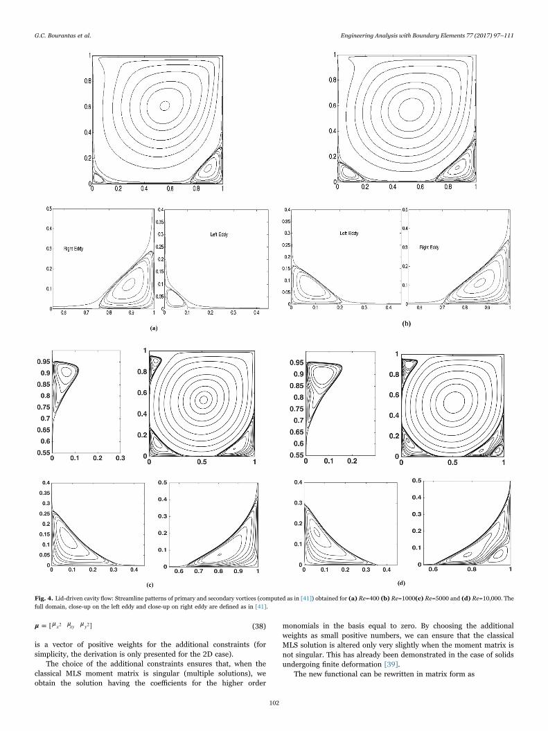
Fig. 4. Lid-driven cavity flow: Streamline patterns of primary and secondary vortices (computed as in [41]) obtained for (a) Re=400 (b) Re=1000(c) Re=5000 and (d) Re=10,000. Thefull domain, close-up on the left eddy and close-up on right eddy are defined as in [41].

G.C. Bourantas et al. Engineering Analysis with Boundary Elements 77 (2017) 97–111

102

Fig. 5. The u-velocity on the section x=0.5 and the v-velocity on the section y=0.5 of the square lid-driven cavity problem for (a) Re=400 (b) Re=1000 (c) Re=5000 and (d)Re=10,000. Results of Ghia et al. [40] are compared with the current numerical solutions.

G.C. Bourantas et al. Engineering Analysis with Boundary Elements 77 (2017) 97–111

103

J Pa u W Pa u a Ha= ( − ) ( − ) + ,MMLS T T (39)

where H is a matrix with all elements equal to zero except the last 3diagonal entries, which are equal to μ:

H μdiag0 00=

( ).33 33

33

⎡⎣⎢

⎤⎦⎥ (40)

Then, following the minimization procedure for the functionalJMMLS used in the classical MLS we get

Fig. 6. (a) Pressure and (b) streamlines contours for the backward-facing step for Re=200.

Fig. 7. Velocity contours for u- component and v- component, respectively for Reynolds number (a) Re=20 and (b) Re=60.

Fig. 8. Pressure contours for (a) Re=20 and (b) Re=60.

G.C. Bourantas et al. Engineering Analysis with Boundary Elements 77 (2017) 97–111

104

Ja

P WP H a x P Wu∂∂

= [ + ] ( ) − =0.MMLS

T T(41)

For the modified moment matrix we can write

M P WP H M H= + = + ,MMLS T (42)

while the new coefficients can be computed as

a x P WP H P Wu( ) = ( + ) .T T1−(43)

Finally, the modified approximant becomes

∑x P P WP H P Wu xu u( ) = ( + ) = Φ ( ) ,T T TMMLS

j

n

jMMLS

j1−

=1 (44)

with the new shape functions

x x x P P WP H P WΦ ( ) = [Φ ( ) … Φ ( )] = ( + ) .T T TMMLS MMLSnMMLS 1

1−

(45)

4. Numerical examples and algorithm verification

We verify the accuracy of the proposed meshless scheme throughseveral flow cases. First, we have considered the two most frequentlyused benchmark problems in Computational Fluid Dynamics (CFD),the lid-driven cavity flow and the backward-facing step (BFS). Next, weexamined flow cases in irregular geometries, starting with a 2Drectangular duct with a cylinder (and multiple cylinders) as an obstacleand a geometry that resembles flow in a blood vessel. Finally, we haveconsidered the 3D lid-driven cavity flow problem as well as a typical 3Dgeometry of a dilated vessel (aneurysm), obtained by segmenting CT(computed tomography) images. For the test cases presented weconsidered Reynolds numbers that correspond to steady state solu-tions. In detail, for the lid-driven cavity flow problem steady statesolutions can be obtained for Reynolds number up to Re=10,000; forthe rest of the flow cases we considered moderate Reynolds numbers toensure steady state solutions. Additionally, moderate Reynolds num-bers ensure, for the flow cases considered in the present study, laminarflow; this is compatible with the flow equations being solved, which areonly valid for laminar incompressible flows.

For the simulations conducted we have used two types of nodalconfigurations: (i) a uniform semi-staggered grid (Type-I) embedded inthe geometry and (ii) a semi-staggered grid (Type-II) based on atriangular (or tetrahedral in 3D) mesh of the spatial domain. Thevertices of the nodes correspond to the velocity nodes, while thebarycenter of triangles to the pressure nodes (this configurationresembles the mini-elements configuration used in FEM). Fig. 1 showsthe nodal configurations used for the case of an irregular geometry. Itworth mentioning that results were also computed for collocated nodaldistribution, where velocity and pressure values are computed on thesame nodes.

4.1. Lid-driven cavity problem

The flow in closed cavities, mechanically driven by tangentiallymoving walls, is a well-known benchmark problem for viscous incom-pressible flow. The forced convection in a square cavity with isothermalsides and moving upper side is known as the lid-driven cavity problem.The lid-driven cavity flow problem, despite its geometrical simplicity, isconsidered to be a challenging problem, mainly due to the vortices thatappear at the corners of the square cavity, especially for high Reynoldsnumbers. The flow boundary conditions imposed were no-slip bound-ary condition for all walls of the cavity, except for the top wall whichmoves with velocity u=1 in the x-direction.

For all the simulations conducted we consider both uniform andirregular nodal distributions previously described. For the constructionof the shape functions and derivatives, in the case of uniform nodaldistribution, the support domain was defined by using the 20 nearestneighbors, while in the case of irregular nodal distribution, an adaptivecut-off radius has been used, adapting accordingly to the number ofnodes in the support domain. Coarse and fine nodal configurationswere used in order to obtain a grid-independent solution.

In the case of uniform nodal distribution (Type-I), a uniform121 × 121 grid (for velocity components) was used for Re=100, whilefor Re=400 and Re=1,000 a 241 × 241 grid was used. Although, nodaldistributions as coarse as 41 × 41 and 81 × 81 were adequate for theconvergence and accuracy of the numerical solution. Additionally,computations were conducted for higher values of the Reynoldsnumber up to Re=10,000, using a uniform nodal distribution of401 × 401 nodes. The results obtained were compared against the

Fig. 9. u- velocity components profile along the line x=0.25 and x=0.3 for Re=20. Solidline is for IPOT-MMLS scheme and squre symbol for COMSOL.

G.C. Bourantas et al. Engineering Analysis with Boundary Elements 77 (2017) 97–111

105

values provided in Ghia et al. [40] at the centerlines (x=0.5 and y=0.5),with the convergence curve of Linf (the maximum absolute value of thedifference between the two solutions) and L2 (the mean square value ofthe difference between the two solutions) shown in Fig. 2. We assess

the accuracy of the method for Re=400, 1000, 5000 and 10,000through qualitative and quantitative comparisons with benchmarknumerical results from the literature [40,41]. For qualitative evaluationof the solution, pressure contours (Fig. 3) and streamlines (Fig. 4,computed as in [41]) of the flow field are presented for Re=400, 1000,5000 and 10,000. The streamlines plotted in Fig. 4 show the formationof the counter-rotating secondary vortices that appear as the Reynoldsnumber increases. For quantitative comparison, we plot the u-velocityprofiles along a vertical line and the v- velocity profiles along ahorizontal line passing through the geometric center of the cavity,respectively, in Fig. 5, for Re=400, 1000, 5000 and 10000. Theseprofiles are in good agreement with of the results from Ghia et al. [40],shown by symbols in Fig. 5.

In the case of irregular nodal distribution (Type-II), trianglevertices were used as the nodal distribution where velocity values arecalculated. Pressure values were calculated at the barycenter of eachtriangular element. For the case of Re=100 we started using a coarsegrid consisting of 2601 velocity nodes and 5000 pressure nodes andgradually refined the grid. The IPOT-MMLS scheme converges to thedata obtained for the benchmark problem. For every type of nodaldistribution, as the number of nodes in the support domain increases,the accuracy of the proposed scheme increases.

4.2. Backward facing step (BFS) problem

The second benchmark problem considered is the backward-facingstep (BFS) flow problem [42]. The flow domain is a channel of width H(H=1) and length L (L=30 H), with an obstacle (step) (of height H=0.5)placed at the left-most edge of the inlet (x=0). Flow is assumed to befully developed, with a parabolic inflow velocity profile given byu=(12y−24y2, 0) for y > 0.5. Fully developed flow is also assumed atthe outlet (right edge), with the velocity profile given by u=(0.75–3y2,0) for 0 < y < 1. At the bottom and top walls no-slip boundary

Fig. 10. Velocity contours for (a) u- component and (b) v- component, for Re=20.

Fig. 11. Pressure contours for Re=20.

Fig. 12. u- velocity components profile along the line x=0.65 and x=0.95 for Re=20.Solid line is for IPOT-MMLS scheme and squre symbol for COMSOL.

Inlet Outlet

Fig. 13. Irregular geometry that resembles a 2D stenosed artery with a bypass.

G.C. Bourantas et al. Engineering Analysis with Boundary Elements 77 (2017) 97–111

106

conditions were imposed.BFS is considered as a demanding benchmark flow problem due to

the vortices formed downstream, just after the step. The BFS has beenstudied both experimentally [42] and numerically [42–45]. The flowhas been found to be stable and two-dimensional for Reynolds numberRe < 400, allowing the flow to be numerically modeled in 2D andcompared directly with experiments [42]. Beyond this Reynoldsnumber, the flow is 3D and the 2D approximation is no longer valid.However, numerical results for the 2D problem for Re > 400 are stillgiven in the literature as a purely numerical benchmark problem [43].Here we present numerical results for our method for Re=200, forcomparison with both experimental and numerical results such as [42].

Initially we tested the performance of the proposed scheme usingthe Type-I nodal distribution. To ensure a grid-independent numericalsolution, successively increasing nodal configurations were testedstarting from 300 × 11, 600 × 21, 900 × 31and 1200 × 41. For theRe=200, a uniform nodal distribution of 27,931 (900 × 31) is used.Fig. 6 shows the streamlines and vorticity contours for Re=200. We canobserve that the flow separates at the step corner and a vortex isformed downstream. For Re=200 the reattachment length of the

formed vortex is Lreattachment=2.55, being in agreement with thatcomputed using different numerical methods, such as MeshlessCollocation Point with Radial Basis Functions and Finite ElementMethod [25]. Type-II nodal configurations were also used, startingfrom a coarse distribution and resulting in a denser one after successiverefinements (total number of nodes used were 12,321). The numericalresults obtained showed excellent agreement with those of Type-I. Forthe case of Re=200 the reattachment length computed wasLreattachment=2.54.

4.3. Flow behind cylinder

In the next example we consider the laminar flow in a rectangularduct with a cylindrical obstacle. The duct has length L=2.2 m andheight H=0.41 m. The cylindrical obstacle is located at point O(0.2,0.2) having radius r=0.05 m. The kinematic viscosity of the fluid wasset to v=0.001 m2/s. The Reynolds number is defined by Re=2ur/vwith the mean velocity umean=(2/3)*u(0,H/2). The inflow conditionsare

Fig. 14. For the bypass geometry (a) pressure contours (b) u- velocity component contours (c) v- velocity component contours(d) streamlines for Re=20 and (e) pressure contours (f)u- velocity component contours (g) v- velocity component contours (h) streamlines for Re=240.

G.C. Bourantas et al. Engineering Analysis with Boundary Elements 77 (2017) 97–111

107

u v u y H yH

( (y), ) = (4 − ,0)m 2

⎛⎝⎜

⎞⎠⎟ (36)

with um=0.3 m/s yielding Reynolds number Re=20. At the outlet afully developed flow u x(∂ /∂ =0) is applied, while at the rest of theboundaries no-slip conditions were applied. Simulations were con-ducted using the different types of nodal configuration described above.The numerical results obtained were compared point wise with thosecomputed using COMSOL [46]. The maximum absolute values of thedifference between the two solutions Linf, for the velocity componentsu- and v-, were computed as 1.14x10−3and 1.82x10−3, respectively. Theuniform semi-staggered nodal distribution (Type-I) was more stable interms of computing shape functions and derivatives. The positivityconditions [47] were fulfilled naturally, in contrast to the Type-IIconfiguration, where extra care should be taken in order to find theoptimal support domain.

For the results obtained using the uniform semi-staggered distribu-tion, the contour plots of the velocity components are shown in Fig. 7,and pressure contours in Fig. 8. We used 9546 nodes with 90 of themdistributed over the cylinder circumference. Finally, Fig. 9 shows u-velocity profile along the line x=0.25 and x=0.3 for Re=20 comparingthe results of IPOT-MMLS technique and COMSOL. All flow variablesare computed in SI units. Contour plots of the velocity components andpressure are presented for Reynolds number up to Re=60 (um=0.9 m/s). For higher values of maximum inlet velocity um, and, consequentlyfor higher values of Re, the flow regime becomes oscillating down-stream and is not considered as steady state flow.

Additionally, we consider the case where a number of cylinders arepresent downstream, using the exact same boundary conditions as inthe case of a single cylinder. In total 18,362 nodes were used, 630 ofthem located on the boundaries. The cut-off radius was chosen suchthat 40 nodes were located in the support domain. The numericalresults obtained were compared against those computed usingCOMSOL, with the maximum absolute values of the difference betweenthe two solutions for the velocity components u- and v- computed as1.2x10−3and 2.3x10−3, respectively. The contour plots for the velocity

u=1, v=0, w=0

x

z

y

Fig. 15. Geometry of the lid-driven flow in a cubic cavity.

Table 1Comparison of numerical results for lid-driven flow in a cubic cavity. u-component of thevelocity profile at the mid-planes for Re=100.

y Ding et al. [48] IPOT-MMLS error Relative error (%)

0.000.040.080.120.160.200.240.280.320.360.400.440.480.520.560.600.640.680.720.760.800.840.880.920.961.00

0−0.028−0.052−0.073−0.092−0.112−0.130−0.148−0.166−0.181−0.194−0.202−0.205−0.202−0.191−0.173−0.147−0.113−0.071−0.0190.0480.1400.2700.4560.7071.000

0−0.025−0.047−0.066−0.084−0.101−0.118−0.135−0.152−0.167−0.180−0.190−0.196−0.197−0.190−0.175−0.152−0.118−0.075−0.0180.0520.1510.2830.4650.7201.000

00.0030.0050.0070.0080.0110.0120.0130.0140.0140.0140.0120.0090.0050.0010.0020.0050.0050.0040.0010.0040.0110.0130.0090.0130

10.79.619.598.699.829.238.788.437.737.225.944.392.470.521.153.404.425.635.268.337.864.811.971.84

Fig. 16. Velocity component distribution along the vertical centerline of cubic cavity, u-yfor (a) Re=100 and (b) Re=400 using successively denser nodal distributions. Squaresymbol is for the results in [48].

Inlet Outlet

Fig. 17. 3D geometry obtained using a CT scan showing the part of the blood vessel thatsuffers from an aneurysm.

G.C. Bourantas et al. Engineering Analysis with Boundary Elements 77 (2017) 97–111

108

components are shown in Fig. 10, while pressure contours are plottedin Fig. 11. Fig. 12 shows u- velocity profile along the line x=0.25 andx=0.3 for Re=20 comparing the results of IPOT-MMLS technique andCOMSOL, when using a staggered grid based on irregular nodaldistribution obtained from a triangular mesh. The 40 closest nodeswere used to define the support domain of each node.

4.4. Bypass geometry

As a fourth example, we consider the flow in an irregular geometrythat resembles a 2D stenosed artery with a bypass, Fig. 13, havinglength of 15 cm. For the simulations conducted, we considered aparabolic velocity profile with u=4um(y-y2) and v=0 in the inlet ofthe domain, at the outlet fully developed flow, and on the remainingwalls no-slip boundary conditions (u=v=0). For um=0.1 m/s andkinematic viscosity of v=0.001 m2/s the Reynolds number was calcu-lated as Re=40, giving rise to laminar flow regime. The proposedscheme can provide accurate results for higher Reynolds numbers; inthe case of v=0.0001 m2/s Reynolds number becomes Re=240. Forhigher Re numbers turbulence may probably occur. Since studyingturbulence is out of the scope of the present study, we restricted thepresented results to low and moderate Reynolds numbers.

Both nodal configuration types were used in order to test the

applicability of the proposed scheme in flow cases concerning irregulardomains. All the numerical solutions, obtained using different nodaldistribution types, converged. The numerical results computed areaccurate as compared to the results obtained using the finite elementmethod (COMSOL). The maximum absolute values of the differencebetween the two solutions for the velocity components u- and v- werecomputed as 2.4x10−3 and 3.6x10−3, respectively. Simulations show thatthe most reliable, in terms of computational cost, stability andconvergence, has been the uniform semi-staggered embedded distribu-tion. Several grids with increasing resolution were used in order toobtain a grid independent solution. For the simulations conducted weused a total of 14,563 nodes, with 1380 of them located on theboundaries. Fig. 14 shows iso-contours for the velocity components u,v, pressure and streamlines. All flow variables are computed in SI units.

4.5. Lid-driven flow in 3D

The lid-driven flow in a cubic cavity (0,1)3 is the natural extensionto 3D of the 2D driven cavity test case, Fig. 15. Numerical results wereobtained for Re=100 and Re=400. A grid independence study has beenconducted to ensure a grid independent numerical solution. Typicalnodal distributions up to 41×41×41 (68,000) and 61×61×61 (226,981)points for Re=100 and 400, respectively, are employed. The numericalresults obtained are in a good agreement with those in [48], Table 1.Velocity profile at the mid-planes for Re=100 and 400, using succes-sively denser nodal distributions, are shown in Fig. 16.

4.6. Flow in 3D aneurysm

We considered the flow in a 3D geometry obtained using a CT scanshowing the part of the blood vessel that suffers from an aneurysm,Fig. 17. The aneurysmatic part of the vessel has been smoothed duringthe segmentation and 3D reconstruction procedure, and the finaloutput was an STL file with all the geometrical information. The lengthof the vessel is L=10 cm and the radius is R=1 cm. Concerning theboundary conditions imposed, at the inlet a plug flow velocity profile(u=1 cm/s, v=w=0), and at the outlet a zero axial velocity gradient wasimposed u x(∂ /∂ =0). On the rest of the boundaries no-slip conditionswere applied. The 3D mesh, consisting of tetrahedral elements, hasbeen created in ANSYS ICEM, the pre-processor contained in ANSYSCFX commercial software [49].

For the simulations conducted the STL file used, shown in Fig. 18a,describes the surface of the vessel geometry, which is represented bytriangles and forming a convex surface. All types of nodal configura-tions described above were used in the simulations conducted. In thecase of the uniform grid embedded in the geometry, a grid-independentsolution was obtained by successively increasing the number of nodes.The numerical solution was compared against the numerical solutiongiven by ANSYS CFX. For the simulations conducted, the distance h ofthe support domain was set to h=0.2 cm (30 nodes in the supportdomain), with a total of 12,456 nodes used inthe computations. Bycomparing the IPOT-MMLS results with those computed by ANSYSCFX, the maximum absolute values of the difference between the twosolutions were 1.2x10−3, 2.3x10−3and 3.6x10−3for u-, v- and w- velocitycomponents, respectively.

In order to depict the direct applicability of the proposed scheme incases where the nodal distributions are directly given using a tetra-hedral mesh, we considered a Type-II nodal distribution,with the nodesof the tetrahedral mesh are used for the computation of the velocityfield values. The pressure field values were computed at the barycenterof the tetrahedral elements. The velocity nodes are shown in Fig. 18band the pressure nodes in Fig. 18c. The pressure contours on thesurface of the vessel are shown in Fig. 19a, while streamlines areplotted in Fig. 19b (in a view angle suitable for streamlines in 3D). Allflow variables are computed in SI units.

Fig. 18. (a) Surface triangulation of the vessel geometry and nodal distribution for (b)velocity (c) pressure field values.

Fig. 19. (a) Pressure contours on the vessel wall and (b) streamlines (in a view anglesuitable for streamlines in 3D) for Re=80.

G.C. Bourantas et al. Engineering Analysis with Boundary Elements 77 (2017) 97–111

109

5. Conclusions

In this paper we applied the Modified Moving Least Squares(MMLS) meshless method in the numerical solution of laminar,incompressible, steady state flow in the context of a point collocationmethod. We solved the flow governing equations in their primitivevariables (velocity-pressure) formulation, by using a semi-staggeredmeshless nodal distribution. A pressure correction methodology (IPOTmethod) has been used in order to fulfil the incompressibility con-straint, ensuring the mass conservation. The advantages of theproposed IPOT meshless point collocation are that it is straightforwardand easy to apply, results can be obtained using collocated or semi-staggered nodal distributions, it works for 2D and 3D geometries, it istruly meshless, while there is no need for pressure boundary conditionssince no pressure constitutive equation is solved. Additionally, in ourapproach there is no need for the computation of the velocity potentialor unit normal vectors. The proposed scheme can be used for thenumerical solution of the transient Navier-Stokes equations; theiterative procedure, used to update the solution in the steady stateequations, can be used to update in time the numerical solution whenan explicit or an implicit solver is used. Additionally, the method isuseful for the flow cases where pressure boundary conditions cannot bedefined. The absence of pressure boundary conditions can be handledby the IPOT scheme. In case where the pressure on the boundaries isknown the IPOT method can also be applied. Nevertheless, for the lastcase more numerical studies are needed.

The MMLS approximation method makes use of two distinct sets ofnodes for velocity and pressure variables. We have focused on themethod's performance, accuracy and stability using uniformly andirregularly distributed nodes. First, we showed that the proposedscheme provides accurate results in uniform geometries using bench-mark fluid flow problems, namely the lid-driven cavity and the back-ward-facing step. Both qualitative and quantitative results were givenin order to show the accuracy of the method used. Second, we testedthe numerical stability and performance of the method across complex-geometry problems. COMSOL and ANSYS CFX were used as referencesolvers for the complex geometries, demonstrating that the proposedscheme provides consistent results across all the problems considered.Concerning the parameters related to upwinding for moderateReynolds numbers, in both COMSOL and ANSYS CFX, the defaultparameters have been used in all the test cases considered. MMLSnumerical scheme was stable with both uniform and irregular nodaldistributions.

Our results show that the use of MMLS operators in conjunctionwith velocity and pressure correction method provide stable andaccurate solutions across a range of 2D and 3D problems, in bothregular and irregular geometries. For every type of nodal distribution,as the number of nodes in the support domain increases, the accuracyof the proposed scheme increases. The same happens when the totalnumber of nodes in the spatial domain is increased, where uniformnodal distributions embedded in geometry seem to be more efficient.Finally, for future applications, the proposed scheme will be upgradedto treat time dependent flow problems, pressure-driven and shear-driven flow, considering flow regimes with high Reynolds number.

Acknowledgments

The financial support of Australian Research Council (DiscoveryGrant no. DP160100714) is gratefully acknowledged. We wish toacknowledge the Raine Medical Research Foundation for funding G.R. Joldes through a Raine Priming Grant.

References

[1] Orszag SA, Israeli M, Deville MO. Boundary conditions for incompressible flows. JSci Comput 1986;1, [175-111].

[2] Ferziger JH, Peric M. Computational methods for fluid dynamics. Springer; 2002.[3] Harlow FH, Welch JE. Numerical calculation of time-dependent viscous incom-

pressible flow of fluid with free surface. Phys Fluids 1965;8:2182–9.[4] Chorin AJ. Numerical solution of the Navier–Stokes equations. Math Comp

1968;22:745–62.[5] de Vries G, Norrie DH. The application of the finite-element technique to potential

flow problems. J Appl Mech ASME Trans 1971;38:798–802.[6] Zienkiewicz OC, Taylor RL, Nithiarasu P. The finite element method for fluid

dynamics, Sixth ed. Butterworth-Heinemann: Elsevier; 2005.[7] Gresho PM, Sani RL. Incompressible Flow and the Finite Element Method. Wiley;

1998.[8] Patankar SV, Spalding DB. A calculation procedure for heat, mass and momentum

transfer in three-dimensional parabolic flows. Int J Heat Mass Transf1972;15:1787–806.

[9] Patankar SV. Numerical heat transfer and fluid flow. New York: McGraw-Hill;1980.

[10] Chorin AJ. A numerical method for solving incompressible viscous flow problems. JComput Phys 1967;2:21–6.

[11] Papadopoulos PK, Hatzikonstantinou PM. Improved CVP scheme for laminarincompressible flows. Int J Numer Methods Fluids 2011;65:1115–32.

[12] Hafez M, Shatalov A, Wahba E. Numerical simulations of incompressible aero-dynamic flows using viscous/inviscid interaction procedures. Comput MethodsAppl Mech Eng 2006;195:3110–27.

[13] Papadopoulos PK. An auxiliary potential velocity method for incompressibleviscous flow. Comput Fluids 2011;51:60–7.

[14] Papadopoulos PK. An implicit potential method for incompressible flows. Int JNumer Methods Eng 2013;94:672–86.

[15] Nguyena VPh, Rabczuk T, Bordas S, Duflot M. Meshless methods: a review andcomputer implementation aspects. Math Comput Simul 2008;79:763–813.

[16] Lin Η, Atluri SN. The meshless local Petrov-Galerkin (MLPG) method for solvingincompressible Navier-Stokes equations. Comput Model Eng Sci 2001;2:117–42.

[17] Mohammadi MH. Stabilized Meshless Local Petrov-Galerkin (MLPG) method forincompressible viscous fluid flows. Comput Model Eng Sci 2008;29:75–94.

[18] Arefmanesh A, Najafi M, Abdi H. Meshless local petrov-galerkin method with unitytest function for non-isothermal fluid flow. Comput Model Eng Sci 2008;25:9–22.

[19] Loukopoulos VC, Bourantas GC. MLPG6 for the solution of incompressible flowequations. Comput Model Eng Sci 2012;88:531–58.

[20] Baez E, Nicolas A. Recirculation of viscous incompressible flows in enclosures.Comput Model Eng Sci 2009;41:107–30.

[21] Grimaldi A, Pascazio G, Napolitano M. A parallel multi-block method for theunsteady vorticity-velocity equations. Comput Model Eng Sci 2006;14:45–56.

[22] Sellountos EJ, Sequeira A. An advanced meshless LBIE/RBF method for solvingtwo-dimensional incompressible fluid flows. Comput Mech 2008;41:617–31.

[23] Sellountos EJ, Sequeira A. Hybrid multi-region BEM/LBEI-RBF velocity-vorticityscheme for the two-dimensional Navier-Stokes equations. Comput Model Eng Sci2008;23:127–47.

[24] Bourantas GC, Skouras ED, Loukopoulos VC, Nikiforidis GC. Meshfree pointcollocation schemes for 2D steady state incompressible Navier–Stokes equations invelocity-vorticity formulation for high values of Reynolds number. Comput ModelEng Sci 2010;59:1–33.

[25] Bourantas GC, Skouras ED, Loukopoulos VC, Nikiforidis GC. Numerical solution ofnon-isothermal fluid flows using local radial basis functions (LRBF) interpolationand a velocity-correction method. Comput Model Eng Sci 2010;64:187–212.

[26] Bourantas GC, Loukopoulos VC. A meshless scheme for incompressible fluid flowusing a velocity-pressure correction method. Comput Fluids 2013;88:189–99.

[27] Kosec G, Šarler B. Solution of thermo-fluid problems by collocation with localpressure correction. Int J Numer Methods Heat Fluid Flow 2008;18:868–82.

[28] Mai-Duy N, Mai-Cao L, Tran-Cong T. Computation of transient viscous flows usingindirect radial basic function networks. Comput Model Eng Sci 2007;18:59–77.

[29] Zhang L, Ouyang J, Zhang XH. On a two-level element-free Galerkin method forincompressible fluid flow. Appl Numer Math 2009;59:1894–904.

[30] Huerta A, Vidal Y, Villon P. Pseudo-divergence-free element free Galerkin methodfor incompressible fluid flow. Comput Methods Appl Mech Eng 2004;193:1119–36.

[31] Shadloo MS, Zainali A, Sadek SH, Yildiz M. Improved incompressible smoothedparticle hydrodynamics method for simulating flow around bluff bodies. ComputMethods Appl Mech Eng 2011;200:1008–20.

[32] Napoli E, De Marchis M, Vitanza E. PANORMUS-SPH. A new smoothed particlehydrodynamics solver for incompressible flows. Comput Fluids 2015;106:185–95.

[33] Ellero M, Serrano M, Espanol P. Incompressible smoothed particle hydrodynamics.J Comput Phys 2007;226:1731–52.

[34] Oñate E, Idelsohn S, Zienkiewicz OC, Taylor RL, Sacco C. A stabilized finite pointmethod for analysis of fluid mechanics problems. Comput Methods Appl Mech Eng1996;139:315–46.

[35] Tiwari S, Kuhnert J. Finite pointset method based on the projection method forsimulations of the incompressible Navier-Stokes equations. Lect Notes Comput SciEng 2003;26:373–88.

[36] Tiwari S, Kuhnert J. Modeling of two-phase flows with surface tension by finitepointset method (FPM). J Comput Appl Math 2007;203:376–86.

[37] Lancaster P, Salkauskas K. Surfaces generated by moving least squares method.Math Comput 1981;37:141–58.

[38] Joldes GR, Chowdhuty HA, Wittek A, Doyle B, Miller K. Modified moving leastsquares with polynomial bases for scattered data approximation. Appl MathComput 2015;266:893–902.

[39] Chowdhury H, Joldes G, Wittek A, Doyle B, Pasternak E, Miller K. Implementationof a modified moving least squares approximation for predicting soft tissuedeformation using a meshless method. In: Doyle B, Miller K, Wittek A, Nielsen

G.C. Bourantas et al. Engineering Analysis with Boundary Elements 77 (2017) 97–111

110

PMF, editors. Computational biomechanics for medicine. Springer InternationalPublishing; 2015. p. 59–71.

[40] Ghia U, Ghia KN, Shin CT. High-Re solutions for incompressible flow using theNavier-Stokes equations and a multigrid method. J Comput Phys1982;48:387–411.

[41] Erturk E, Corke TC, Gokcol C. Numerical solutions of 2-D steady incompressibledriven cavity flow at high Reynolds numbers. Int J Numer Methods Fluids2005;48:747–74.

[42] Armaly BF, Durst F, Pereira JCF, Schonung B. Experimental and theoreticalinvestigation of backward-facing step flow. J Fluid Mech 1983;172:473–96.

[43] Gartling DK. A test problem for outflow boundary conditions – flow over abackward-facing step. Int J Numer Methods Fluids 1990;11:953–67.

[44] Kim J, Moin P. Application of a fractional-step method to incompressible Navier-Stokes equations. J Comput Phys 1985;59:308–23.

[45] Sohn J. Evaluation of fidap on some classical laminar and turbulent benchmarks.Int J Numer Methods Fluids 1988;8:1469–90.

[46] COMSOL Multiphysics product.[47] Jin X, Li G, Aluru NR. Positivity conditions in meshless collocation methods.

Comput Methods Appl Mech Eng 2004;193:1171–202.[48] Ding H, Shu C, Yeo KS, Xu D. Numerical computation of three-dimensional

incompressible viscous flows in the primitive variable form by local multiquadricdifferential quadrature method. Comput Methods Appl Mech Eng2006;195:516–33.

[49] ANSYS® Academic Research.

G.C. Bourantas et al. Engineering Analysis with Boundary Elements 77 (2017) 97–111

111