CONSISTENT NON-REFLECTING BOUNDARY … · related disciplines like aeroelasticity and aeroacoustics, ... Straightforward far-ﬁeld or simple 1D characteristic boundary conditions

ECCOMAS Congress 2016VII European Congress on Computational Methods in Applied Sciences and Engineering

M. Papadrakakis, V. Papadopoulos, G. Stefanou, V. Plevris (eds.)Crete Island, Greece, 5–10 June 2016

CONSISTENT NON-REFLECTING BOUNDARY CONDITIONS FORBOTH STEADY AND UNSTEADY FLOW SIMULATIONS IN

TURBOMACHINERY APPLICATIONS

Daniel Schluß, Christian Frey, Graham Ashcroft

German Aerospace Center (DLR)Institute of Propulsion Technology

Linder Hohe, 51147 Cologne, Germanyemail: [email protected], [email protected], [email protected]

Keywords: Non-Reflecting Boundary Conditions, Turbomachinery, Steady and Unsteady CFD

Abstract. This paper presents the implementation of a non-reflecting boundary condition forsteady and unsteady turbomachinery flow computations. Here, the truncation of the computa-tional domain can lead to spurious numerical reflections due to artificial open boundary sur-faces. To face this issue, Giles introduces a popular set of non-reflecting boundary conditionsfor turbomachinery applications. Whereas the steady formulation is exact within the lineari-sation approach, Giles suggests an approximate boundary condition for unsteady simulations.Resulting from this approximation, the unsteady boundary conditions are not perfectly non-reflecting. Thus, steady and time averaged unsteady flow solutions do not necessarily coincide,even if the flow field contains no unsteadiness.

We suggest a single boundary condition formulation suitable for steady and unsteady sim-ulations. This approach applies a modal decomposition and, thus, undesired incoming modescan easily be ruled out. Steady modes can be handled as in the steady case. Apart from theassumptions made by starting from the linearised, two-dimensional Euler equations, this ap-proach does not require any further approximation, and, therefore, the time-averaged unsteadyand the steady solutions coincide in the limit of steady flows.

We apply and assess the presented boundary condition in steady and unsteady computationsof two turbomachinery test cases.

1


1 INTRODUCTION

Computational fluid dynamics (CFD) based upon the Reynolds-averaged Navier-Stokes equa-tions (RANS) has become a vital tool for both design of and research on turbomachinery ap-plications in the aerospace, energy and automotive industries. Steady computations remain thebackbone of industrial design processes especially due to their extensive utilization in shapeoptimization methods. Unsteady turbomachinery flow simulations, on the other hand, attainincreasing importance for understanding blade row interactions which is needed to achievehigher aerodynamic loads and closer blade row spacings to meet the desire for more efficientand lighter engines. Moreover, these design trends require additional activities in fluid dynamicsrelated disciplines like aeroelasticity and aeroacoustics, which again heavily rely on unsteadyCFD [1, 2].

The quality of flow simulations depends, beside the choice of an appropriate closure modelfor the RANS equations and the properties of the numerical scheme, directly on the boundaryconditions imposed. Straightforward far-field or simple 1D characteristic boundary conditionscan lead to spurious, numerical reflections deteriorating the flow solution inside. Thus, manyaerodynamic problems, such as the flow around an airfoil or wing, are commonly simulated invery large computational domains to minimise the impact of the far-field boundary conditionson the region of interest.

In turbomachinery flows, however, this is usually not possible. Firstly, instead of the wholemachine, only single components or certain sets of stages or blade rows are considered whichleads to artificial, open boundaries rather close to the blades. Additionally in steady turboma-chinery CFD, adjacent blade rows in their respective relative frames of reference are coupledvia so-called mixing planes [3]. These mixing planes pose boundary conditions to the adja-cent domains which strengthens the need for non-reflecting boundary conditions (NRBC) inturbomachinery applications.

Numerical reflections, that emerge when applying less advanced boundary conditions, candisturb the flow field in the neighbourhood of a blade leading to an incorrect surface pressuredistribution and hence aerodynamic work or losses. We will give an example for this later in theapplication section. In particular, reflecting boundary conditions can deteriorate the predictionof aeroelastic or aeroacoustic phenomena as shown by Kersken et al. [4] and Ashcroft andSchulz [5].

The mathematical theory of non-reflecting boundary conditions is presented in a review pa-per by Hidgon [6]. Based upon this theory, Giles introduces a set of NRBC for 2D turboma-chinery flows [7, 8]. Giles’ approach assumes wavelike perturbations around an average flowstate. Thus, the linearised Euler equations are considered neglecting viscous effects. Trans-forming these perturbations into the spectral, i.e. time and wavenumber, domain and exploitingan eigenvector analysis, one obtains a set of modal perturbations and their respective directionof propagation. This decomposition enables the definition of a flow state at the boundariesthat does not induce undesired incoming perturbations. The straightforward implementationof these NRBC requires the frequencies and wave numbers of all perturbations at the bound-ary to be known. Due to the Fourier transform applied here, these boundary conditions arenon-local in time and space. Therefore, Giles suggests an approximate boundary condition forunsteady computations derived from theoretical work of Engquist and Majda [9]. This boundarycondition is derived from a Taylor series expansion about the ideal one-dimensional boundarycondition and, thus, is local in time and space apart from the fact that it requires averaged quan-tities. A more detailed description of the implementation of these boundary conditions is given

2


in [10]. Saxer and Giles present an extension of the non-local, steady NRBC to 3D flows [11].However, resulting from the approximation, Giles states the unsteady boundary conditions

may produce significant unphysical reflections for outgoing modes with large circumferentialwavenumbers [8]. Accordingly, steady solutions obtained utilizing the exact steady NRBC andtime averaged unsteady flow solutions may differ even for naturally steady flows. Hagstromproposes a higher order approach for the approximation of unsteady NRBC [12]. This methodis local in time but employs a Fourier transform in space. Henninger et al. [13] apply it toacoustic and aeroelastic turbomachinery test cases and demonstrate improved non-reflectingproperties compared to Giles’ boundary condition.

To overcome the inconsistency of steady and unsteady NRBC and ensure their comparabilityin steady and time-accurate turbomachinery flow simulations, the authors propose a boundarycondition formulation suitable for both. This approach applies a modal decomposition in timeand circumferential direction. Thus, the zeroth harmonic in time can be handled by a steadyboundary condition. Disturbances of higher harmonics are treated independently. Accordingly,undesired incoming modes can easily be ruled out. Apart from the assumptions made by startingfrom the linearised, two-dimensional Euler equations, this approach does not require any furtherapproximation, and, therefore, the time-averaged unsteady and the steady solution coincide inthe limit of steady flows.

In this paper, we firstly outline the theory behind NRBC and the approximation made byGiles. Subsequently, we present the implementation of an exact method and apply it to steadyand unsteady turbomachinery computations. In order to validate our implementation of thisboundary condition in DLR’s 3D RANS solver for internal and turbomachinery flows, TRACE,we give a comparison to characteristic and 2D non-reflecting steady boundary conditions andapproximate unsteady 2D NRBC. Thereby, the favourable behaviour of the exact method isdemonstrated.

2 NON-REFLECTING BOUNDARY CONDITIONS

Before presenting our implementation of an exact boundary condition, we want to give abrief overview of one way to construct non-reflecting boundary conditions in the context of tur-bomachinery CFD as they are implemented in TRACE. A more elaborate description includingthe mathematical derivation and well-posedness analysis is given in Giles’ technical report [7]and implementation details can be found in his UNSFLO report [10].

2.1 General approach

For many turbomachinery flows we can assume that variations in pitchwise direction pre-dominate variations in spanwise direction [11]. Thus, we can adapt Giles’ originally two-dimensional formulation for three-dimensional flows as a reasonable approximation. Here, theoriginal technique is applied in blade-to-blade planes, i.e. the coupling of planes of constantrelative channel height is neglected.

Let q = (%, u, v, w, p) be the vector of primitive variables with density %, pressure p and ve-locity components u,v and w aligned such that u is normal to the boundary but in flow directionwhilst v and w point along the boundary in pitchwise and spanwise direction, respectively. Forthe construction of non-reflecting boundary conditions we further consider sufficiently smallperturbations around a mean flow state. So we can linearised the three-dimensional Euler equa-

3


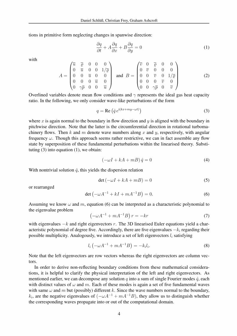
tions in primitive form neglecting changes in spanwise direction:

∂q

∂t+ A

∂q

∂x+B

∂q

∂y= 0 (1)

with

A =

u % 0 0 00 u 0 0 1/%0 0 u 0 00 0 0 u 00 γp 0 0 u

and B =

v 0 % 0 00 v 0 0 00 0 v 0 1/%0 0 0 v 00 0 γp 0 v

(2)

Overlined variables denote mean flow conditions and γ represents the ideal gas heat capacityratio. In the following, we only consider wave-like perturbations of the form

q = Re(q ei(kx+my−ωt)) (3)

where x is again normal to the boundary in flow direction and y is aligned with the boundary inpitchwise direction. Note that the latter is the circumferential direction in rotational turboma-chinery flows. Then k and m denote wave numbers along x and y, respectively, with angularfrequency ω. Though this approach seems rather restrictive, we can in fact assemble any flowstate by superposition of these fundamental perturbations within the linearised theory. Substi-tuting (3) into equation (1), we obtain:

(−ωI + kA+mB) q = 0 (4)

With nontrivial solution q, this yields the dispersion relation

det (−ωI + kA+mB) = 0 (5)or rearranged

det(−ωA−1 + kI +mA−1B

)= 0. (6)

Assuming we know ω and m, equation (6) can be interpreted as a characteristic polynomial tothe eigenvalue problem (

−ωA−1 +mA−1B)r = −kr (7)

with eigenvalues −k and right eigenvectors r. The 3D linearised Euler equations yield a char-acteristic polynomial of degree five. Accordingly, there are five eigenvalues−ki regarding theirpossible multiplicity. Analogously, we introduce a set of left eigenvectors li satisfying

li(−ωA−1 +mA−1B

)= −kili. (8)

Note that the left eigenvectors are row vectors whereas the right eigenvectors are column vec-tors.

In order to derive non-reflecting boundary conditions from these mathematical considera-tions, it is helpful to clarify the physical interpretation of the left and right eigenvectors. Asmentioned earlier, we can decompose any solution q into a sum of single Fourier modes q, eachwith distinct values of ω and m. Each of these modes is again a set of five fundamental waveswith same ω and m but (possibly) different k. Since the wave numbers normal to the boundary,ki, are the negative eigenvalues of (−ωA−1 +mA−1B), they allow us to distinguish whetherthe corresponding waves propagate into or out of the computational domain.

4


The change in primitive variables induced by such a wave is expressed by the respective righteigenvector ri. In other words, the right eigenvectors form a set of linearly independent basisvectors and every perturbation from a mean state can be decomposed into a linear combinationof right eigenvectors with weights αi :

q = Re

([5∑i=1

αirieikix

]ei(my−ωt)

)(9)

For different eigenvalues ki 6= kj , each left eigenvector li is orthogonal to rj , i.e. lirj = 0.For eigenvalues of multiplicity larger than one, the corresponding eigenvectors can be con-structed such that lirj = 0 for i 6= j. Because of this perpendicularity relation, the left eigen-vectors help us to determine the share of their corresponding right eigenvector in any arbitraryperturbation, i.e. αi = liq. So the pivotal idea for the construction of non-reflecting boundaryconditions is to decompose the flow state at a boundary and rule out the incoming waves. Thiscan be done by requiring for any combination of ω and m

liq = 0 (10)

for each li belonging to an incoming wave .Applying the above to the three-dimensional linearised Euler equations, we obtain the fol-

lowing wave numbers:

k1,2,3 =ω −mv

u(11)

k4 =(ω −mv) (aΨ− u)

a2 − u2 (12)

k5 = −(ω −mv) (aΨ + u)

a2 − u2 (13)

with speed of sound a and

Ψ =

{√∆ if ∆ > 0,

−i sign (ω −mv)√−∆ if ∆ < 0

(14)

and

∆ = 1− (a2 − u2)m2

(ω −mv)2. (15)

The wave numbers k1,2,3 are real and the group velocity normal to the boundary ∂ω∂k

= u ispositive. Thus, the respective perturbations r1,2,3 propagate convectively in flow direction. Theyare incoming waves at an inflow boundary and outgoing ones at an outflow. The calculationof k4 and k5 requires the distinction of two cases. If ∆ > 0 then Ψ is real. For flows thatare subsonic normal to the boundary it can be shown that one wave is incoming and one isoutgoing. Taking the positive branch of the root yields the wave corresponding to k4 alsopropagates in flow direction whereas the other one travels in the opposite direction. If ∆ <0, Ψ becomes complex. We choose the sign of Ψ such that Im(k4) is real and, according toequation (3), the corresponding wave propagates downstream, which is consistent with the case∆ > 0. The wave associated with k5 then again travels upstream. In the particular case of

5


∆ = 0, acoustic resonance occurs, which involves additional challenges for the construction ofboundary conditions [4, 14]. But this case is not considered in the present work.

For flows that are supersonic normal to the boundary, there is no upstream running wave.Yet, there are only very few axially supersonic turbomachinery applications and, secondly, su-personic inflow and outflow boundary conditions are rather straightforward and can be found inmany textbooks on CFD (e.g. [15]). Hence, this paper does not consider boundary conditionsfor normally supersonic flows.

To write down the eigenvectors and formulate boundary conditions based upon them, it isconvenient to define

λ =m

ω. (16)

The matrix of right eigenvectors R = (r1 r2 r3 r4 r5) is defined by:

R (λ) =

−% 0 0 %(1−(1−vλ)MaxΨ)

2(1−Max)%(1+(1−vλ)MaxΨ)

2(1+Max)

0 a uλ 0 a(1−vλ)(Ψ−Max)2(1−Max)

−a(1−vλ)(Ψ+Max)2(1+Max)

0 a (1− vλ) 0a2(1−Ma2x)λ

2(1−Max)

a2(1−Ma2x)λ2(1+Max)

0 0 a 0 0

0 0 0 % a2(1−(1−vλ)MaxΨ)2(1−Max)

% a2(1+(1−vλ)MaxΨ)2(1+Max)

(17)

with Max denoting the boundary normal Mach number. From this, the significance of eachright eigenvalue becomes apparent. As r1 only affects the density, it constitutes an entropyperturbation. The second and third eigenvectors represent vorticity disturbances in the blade-to-blade plane and in spanwise direction, respectively. Since ω−mv

uis a triple eigenvalue of the

dispersion relation (6), the determination of r1, r2 and r3 is not unique. However, choosingthem this way yields a physically vivid set of eigenvectors and their required orthogonalityis evident at once. The two remaining eigenvectors correspond to upstream and downstreamrunning acoustic perturbations, i.e. isentropic, irrotational pressure waves.

The left eigenvector matrix can be derived likewise. Another possibility to obtain the lefteigenvector matrix is to invert the right eigenvector matrix:

L =

l1l2l3l4l5

= R−1 =

−1%

0 0 0 1% a2

0 −uλa

1−vλa

0 −λ% a

0 0 0 1a

0

0 1−vλa

uλa

0 (1−vλ)Ψ

% a2

0 −1−vλa

−uλa

0 (1−vλ)Ψ

% a2

(18)

Due to the fact that there is one outgoing wave at an inflow and four outgoing waves at anoutflow, we need to extrapolate outgoing perturbations from the interior. To do so, we definecharacteristic variables c = (c1 c2 c3 c4 c5)T such that these characteristics coincide with theweights αi in equation (9) for plane waves running perpendicularly to the boundary. Note thisis the case if m = 0 or equivalently λ = 0. Hence, the forward and backward transformationsare given by

c = L1d q (19)

6


with

L1d = L(0) =

−1%

0 0 0 1% a2

0 0 1a

0 00 0 0 1

a0

0 1a

0 0 1% a2

0 − 1a

0 0 1% a2

(20)

andq = R1d c (21)

with

R1d = R(0) =

−% 0 0 %

2%2

0 0 0 a2−a

2

0 a 0 0 00 0 a 0 0

0 0 0 % a2

2% a2

2

. (22)

2.2 Steady boundary conditions

The boundary condition generally consists of two steps, i.e. mean flow conditions and cir-cumferential perturbations are treated separately. As changes in the mean flow represent planewaves at the boundary, we can directly express them by changes in the 1D characteristics. In thefollowing, we write down inflow and outflow boundary conditions by means of characteristicsin a compact form, so equations for in- and outflow boundaries are only given separately wherenecessary. For this purpose, we separate the left and right eigenvector matrices and their cor-responding characteristics depending on the direction of propagation of their associated waves.In normally subsonic flows, the first four waves propagate downstream and the fifth one runsupstream. Accordingly, we write for an inflowLin

Lout

=

l1l2l3l4l5

(23)

cin

cout

=

c1

c2

c3

c4

c5

(24)

(Rin Rout

)=

(r1 r2 r3 r4 r5

)(25)

7


and for an outflow LoutLin

=

l1l2l3l4l5

(26)

coutcin

=

c1

c2

c3

c4

c5

(27)

(Rout Rin

)=

(r1 r2 r3 r4 r5

). (28)

To meet the boundary values specified by the user, we define a residual vector for both inflowand outflow boundaries

Rbd =

p(s− sbd)

% a (v − u tan(αcirc,bd))

% a (w − u tan(αrad,bd))

%(ht − ht,bd)

for inflow boundaries

(p− pbd

)for outflow boundaries

(29)

Here, the subscript bd denotes user specified boundary values. Since for turbomachinery flows,the user commonly specifies stagnation pressure and stagnation temperature at an inflow bound-ary, the associated specific entropy s and specific stagnation enthalpy ht need to be calculatedfrom the former. The angles αcirc and αrad represent the angles between the velocity vector andthe boundary normal in pitchwise and spanwise direction. Mixing planes can be covered bydefining analogously

Rbd = Lin1d δqmp (30)

with δqmp being the difference between the flow states at each side of the mixing plane in thesame frame of reference.

To meet the boundary values specified by the user or mixing plane, the required change ofcharacteristics is obtained via a Newton-Raphson step:

Rbd +∂R

∂q

∂q

∂cinδcin = 0 (31)

Note that ∂q∂cin

is the backward transformation of the incoming characteristics, Rin1d. The deriva-

tion of the residual Jacobian ∂R∂q

can be found in [10]. For the adaption of Giles’ originalboundary condition to a cell-centred solver, where the boundary condition is applied betweentwo pseudo-time updates, we also need to modify the update of the mean charactersistics at thefaces due the pseudo-time change of the outgoing characteristics in the interior [16]. We defineanother residual

Ri = Lout1d (qf − qi) (32)

8


where subscripts i and f denote inner cell values and face values, respectively. Note that theinner values have already been updated by the pseudo-time solver whereas face values are stillabout to be updated by the boundary condition. Finally, the update of mean characteristics reads

δc = −L1d

[Rin

1d

(∂R

∂qRin

1d

)−1

Rbd +Rout1d Ri

](33)

To apply the actual non-reflecting boundary condition, we perform a Fourier decompositionof the disturbances about the mean flow along the boundary in the pitchwise direction. Thespatial transformation for any quantity φ reads

φi =1

P

∫ P

0

φ e−imi y dy. (34)

with wave numbers mi = 2πi+θP6= 0, pitch P , inter-blade phase angle θ and local deviation

from the average state φ = φ − φ. Note that θ vanishes in steady computations. Accordingly,the backward transformation is given by

φ = Re

(∞∑

i=−∞

φi eimi y

). (35)

In order to attain non-reflecting properties at the boundary, equation (10) must be satisfied forevery mode with mi 6= 0 and ω = 0. We can scale the second to fifth left eigenvectors by ω andthen set ω to zero. Consequently, the left eigenvector matrix for steady boundary conditionsreduces to

Ls =

−1%

0 0 0 1% a2

0 − ua2− va2

0 −1% a2

0 0 0 1a

0

0 − va2

ua2

0 β% a3

0 va2

− ua2

0 β% a3

(36)

with

β =

{i sign(m)

√a2 − (u2 + v2) for u2 + v2 < a,

−sign(v)√

(u2 + v2)− a for u2 + v2 > a.(37)

We can express the actual boundary condition, equation (10), in terms of characteristics whichis helpful to write the overall boundary update as a sum of mean characteristic changes andlocal changes. Note that the outgoing characteristics have to be extrapolated from the interior.

Lins q = Lins(Rin

1d Lin1d qf +Rout

1d Lout1d qi

)= Lins

(Rin

1d cinf +Rout

1d couti

)= 0 (38)

The above equation yields ideal values for the incoming characteristics as a function of theoutgoing ones. To meet the ideal values, the required changes in the characteristic at an inflowboundary is given by

δc1

δc2

δc3

δc4

δc5

=

−cf,1

−β+va+u

ci,5 − ci,2−cf,3(

β+va+u

)2ci,5 − cf,4

ci,5 − cf,5

. (39)

9


Accordingly, the outflow boundary condition readsδc1

δc2

δc3

δc4

δc5

=

ci,1 − cf,1ci,2 − cf,2ci,3 − cf,3ci,4 − cf,4

2uβ−v ci,2 −

β+vβ−v ci,4 − cf,5

. (40)

Subsequently, these characteristic changes can be transformed from the wavenumber domainback into the physical domain according to equation (35) yielding a local change of the charac-teristics δc.

For supersonic (u2+v2 > a2), but normally subsonic (u < a) flows, β andLs are independentof m according to equations (36) and (37). Hence, no Fourier transformation is required andequations (39) and (40) can be applied directly at each face substituting any c by c. Note thatthe steady, supersonic boundary conditions become local boundary conditions in this case apartfrom their dependence on averaged quantities.

Prescribing no incoming perturbations means that entropy and enthalpy are uniform alongthe inflow boundary only within the linearised theory, but second-order perturbations may stilloccur. Thus, we replace the condition for δc1 and δc4 in the physical domain and instead enforceuniform entropy and enthalpy by locally driving the following residual(

R1

R2

)=

(p s

%ht

)(41)

to zero. This can be done by means of a Newton-Raphson step(R1

R2

)+

(γRγ−1

p 0 0γγ−1

p % a v %2

(a2 + a u)

)δc1

δc2

δc4

= 0 (42)

where R denotes the specific gas constant. The resulting condition for the update of c1 and c4

reads (δc1

δc4

)=

(−γ−1

γRs

−2a(a+u)

(ht + s

γRa2 + a v δc2

)) . (43)

We further have to determine the integral change of characteristics due to circumferentialperturbations because the mean flow boundary conditions already ensure that averaged flowquantities match the boundary values specified by the user or the mixing plane. Accordingly,we have to subtract the integral change afterwards in order to guarantee the mean change ofcharacteristics is not affected by the treatment of perturbations. For this purpose we introduce

δc =1

P

∫ P

0

δc dy. (44)

Finally, the overall update of a boundary face can be written as

δq =[σRin

1d

(δcin + δcin − δcin

)+Rout

1d

(δcout + δcout − δcout

)]. (45)

The relaxation factor σ, which needs to be chosen suitably in the range of 0 to 1, is necessary toretain the well-posedness of the mathematical problem [7]. For the application in a cell-centredsolver, the updated face values have to be extrapolated appropriately to the ghost cells.

10


2.3 Approximate unsteady boundary conditions

To overcome the disadvantage of the straightforward, exact unsteady NRBC being spatiallyand temporally non-local, Giles proposes an approximate, local unsteady boundary condition[7]. This approach has been introduced by Engquist and Majda for general wave equations [9],but Giles applied it to two-dimensional linearised Euler equations in general and turbomachin-ery flows in particular.

As in steady boundary conditions, the averaged flow field and perturbations are handledseparately. The mean flow boundary condition is identical to the steady mean flow boundarycondition except that averaged quantities in the residual (29) are additionally averaged in timerather than only circumferentially. Unsteady turbomachinery flows are (within the framework ofRANS) considered to be periodic and, therefore, temporal averaging means averaging a quantityover one period in this context.

The actual approximate boundary condition, however, handles perturbations from the meanstate. The condition for a (hypothetically) perfectly non-reflecting boundary treatment has beendiscussed in section 2.1. But the universal application of equations (10) and (18) requires thedecomposition of the boundary flow field into the Fourier domain. To avoid this costly trans-formation, the central concept is to express the exact unsteady boundary condition by use ofa Taylor series expansion about the one-dimensional characteristic boundary condition. Recallfrom equation (16) that λ → 0 and from equations (15) and (14) that Ψ → 1 in the one-dimensional case due to vanishing circumferential wave numbers m. Then, the second orderapproximation of the left eigenvector matrix L reads

La = L|λ=0 + λ∂L

∂λ

∣∣∣∣λ=0

= L1d +m

ω

∂L

∂λ

∣∣∣∣λ=0

. (46)

Now the boundary condition Lina q = 0 can be rearranged starting with multiplying by ω. Com-paring equations (1) and (4), we can infer that we can replace ω by i ∂

∂tand m by −i ∂

∂yyielding

Lin1d∂q

∂t− ∂Lin

∂λ

∣∣∣∣λ=0

∂q

∂y= 0. (47)

Giles’ shows his original formulation may become ill-posed at inflows [7]. To face this ill-posedness, he proposes a modification by giving up the perfect orthogonality of l4 and r5 andthereby the condition for perfect non-reflecting behaviour. A multiple of (λ l2,1d) is added tola,4 such that la,4 r5 is minimized under the constraint of the inflow boundary condition beingwell-posed. Expressing q in terms of characteristics, we can again extrapolate the outgoingcharacteristic c5 from the interior and obtain the following inflow boundary condition

∂

∂t

c1

c2

c4

+

v 0 00 v 1

2(a+ u)

0 12

(a− u) v

∂

∂y

c1

c2

c4

+

012

(a− u)0

∂c5

∂y= 0. (48)

The outflow boundary condition is already well-posed in its original formulation and, thus,remains unchanged. It reads

∂c5

∂t+ v

∂c5

∂t+(0 1

2(a+ u) 0

) ∂∂y

c1

c2

c4

= 0. (49)

11


As the characteristic c3, representing vorticity perturbations in spanwise direction, is decoupledin this quasi-three-dimensional approach, this characteristic is treated as a convective perturba-tion and, hence, extrapolated appropriately.

The appropriate numerical method to solve these differential equations at the boundariesdepends on the solution methods for the flow equations in the interior. The solution algorithmapplied in TRACE is presented in [5]. The primitive variables at the boundary and in the ghostcells are reconstructed from the change of characteristics in the same manner as in the steadyboundary conditions.

Due to the chosen approach, to express the left eigenvector matrix by a Taylor series expan-sion of order two in λ, this boundary is only perfectly non-reflecting for planar waves impingingnormally upon the boundary. In general, the boundary conditions become more reflecting withincreasing λ. Accordingly, flows with large circumferential wave numbers and flows that aredominated by low frequency perturbations can induce spurious reflections at the boundary. Thenon-reflecting properties of the inflow boundary condition are further diminished by the mod-ification to gain well-posedness. Details on reflections coefficients can be found in [7] andapplications to two-dimensional pressure-waves in uniform mean flow assessing the reflectionproperties are presented in [17].

A first order approximation of these boundary conditions is also implemented in TRACE. Inthe application section of this paper, both boundary conditions are applied and compared to theexact approach. Note that the first order approximation can also be regarded as a characteristic,one-dimensional boundary condition.

2.4 Exact NRBC

It can be difficult to distinguish between the impact of approximate, unsteady boundary con-ditions and actual unsteady effects when comparing unsteady and steady flow simulations. Theauthors rank direct comparability of steady and unsteady computations as highly desirable inorder to asses unsteady flow phenomena in turbomachinery design and research. Therefore,we do not consider Fourier transforms in time and space to be necessarily circumvented dueto their computational effort. The fundamental concept of the exact boundary conditions isapplying condition (10) to any incoming mode of the spatially and temporally decomposedboundary flow field. For this purpose, we first determine the temporal Fourier decompositionat the boundary according to the approach He proposed in the context of his phase lag method[18]. For the implementation in TRACE, the reader is referred to [19]. The choice of consideredharmonics is analogous to the phase lag set of harmonics. From here on, we distinguish tem-porally Fourier transformed quantities, denoted by subscript ω, and circumferentially Fouriertransformed quantities, denoted by subscript m. For simplicity, this has been omitted up tothis point. The temporal Fourier coefficients qω are again expressed in terms of characteristicvariables cω = L1dqω. For each frequency in the Fourier domain, the flow can also be Fouriertransformed along the boundary according to equation (34) and the respective outgoing charac-teristics are again extrapolated from the interior characteristics cout(ω,m),i . The exact non-reflectingboundary condition for every mode, i.e. for every combination of ω and m, reads

Linq(ω,m),f = Lin(Rin

1d cin(ω,m),target +Rout

1d cout(ω,m),i

)= 0. (50)

L no longer needs to be approximated because ω andm are known in this context. The conditionfor updating the incoming modal characteristics is

δcin(ω,m) =[−(LinRin

1d

)−1LinRout

1d c(ω,m),i

]− cin(ω,m),f . (51)

12


The outgoing characteristic is modified according to

δcout(ω,m) = cout(ω,m),i − cout(ω,m),f (52)

The mean flow q0,0 is treated in the same manner as in the steady or approximate unsteadyboundary condition according to equation (33).

Transforming δc(ω,m) back into the physical domain, we obtain face-wise, harmonic charac-teristics δcω(y). The change of primitive variables at each face is relaxed again:

δqω = σR1dδcω (53)

Subsequently, the boundary states can be extrapolated to the ghost cells in the frequency do-main. Finally, the current ghost cell state is reconstructed by means of an approximate, inverseFourier transform, again exploiting the phase lag functionality in TRACE [19].

Due to its universal approach, this boundary condition is suitable and consistent for bothsteady and unsteady simulations. Beyond, this approach is perfectly consistent with the non-reflecting boundary condition for frequency domain methods, presented by Frey [20, 21], whichis rather favourable to compare unsteady time-domain computations and frequency domaincomputations. Chassaing and Gerolymos [17] demonstrate the advantageous reflection prop-erties towards Giles’ approximate boundary conditions for certain acoustic waves in uniformmean flow. Yet, they observe considerably slower convergence. This is considered by the au-thors of this paper to be due to the issue of temporal Fourier coefficients evolving rather slowlyover possibly many periods, which is a known handicap of the phase lag approach.

3 APPLICATION

To validate our implementation of the exact boundary conditions and asses their non-reflectingproperties, we show their application to two turbomachinery test cases. The behaviour of theexact NRBC is compared to steady NRBC, first and second order approximate NRBC and sim-ple, one-dimensional, steady Riemann boundary conditions. For the description of Riemannboundary conditions, the reader is referred to [15].

When discussing boundary conditions for turbomachinery flows, the appropriate definitionof a mean state is not trivial. This issue has been excluded from the theory section to stick to theactual subject of non-reflecting boundary conditions. In the following applications, however,all mean flow states are obtained by flux averaging [10] along the pitch and additionally in timefor unsteady flows.

All computations are performed on structured grids using DLR’s finite-volume 3D RANSsolver TRACE [22, 23] applying Roe’s upwind scheme [24] extended to second order accu-racy through van Leer’s MUSCL extrapolation [25] and an appropriate limiter function forconvective fluxes. Viscous fluxes are computed based on gradients obtained by a central finitedifference scheme in combination with Wilcox’s linear eddy viscosity turbulence model [26].For steady simulations a first order implicit pseudo-time marching technique is employed. Thesame pseudo-time method is used for subiterations of single time steps in unsteady computa-tions.

3.1 VKI LS89

The first test case is a two-dimensional, linear turbine cascade designed and investigated atthe von Karman Institute for Fluid Dynamics. The airfoil is typical of high pressure turbinenozzle guide vanes. A detailed description can be found in [27].

13


(a) exact NRBCsteady computation

(b) steady NRBCsteady computation

(c) 1D Riemannsteady computation

(d) exact NRBCunsteady computation

(e) 2nd order approx. BCunsteady computation

(f) exact NRBCsteady computationlong domain

(g) steady NRBCsteady computationlong domain

Figure 1: Pseudo-Schlieren images obtained by plotting density gradient magnitude (black corresponds to largegradients)

All calculations are carried out for a supercritical operating point with 415 K stagnationtemperature and 147500 Pa stagnation pressure at the inlet and 78000 Pa static pressure at theoutlet. The inflow is purely axial. Steady computations are conducted applying one-dimensionalRiemann boundary conditions, steady NRBC and exact NRBC.

Unsteady computations apply the second order approximate boundary conditions and theexact NRBC. The base frequency is set to 6100 Hz. The underlying assumption is that a down-stream rotor blade with the same pitch faces purely axial flow in its relative frame of referenceat this blade passing frequency. Therefore, this frequency is estimated to have a realistic or-der of magnitude for turbomachinery flows. One period is resolved by 64 time steps using asecond order Euler backward scheme. For every physical time step, 25 pseudo-time iterationsare performed. Though we perform unsteady computations, both solutions converge to a steadystate.

Inlet and outlet planes are located at 50 % axial chord length away from the leading and

14


training edge. The computational grid comprises 21016 cells. Furthermore, we conduct steadycomputations with axial spacing between boundaries and the blade of 300 % axial chord lengthapplying steady and exact NRBC to produce reference results. The extended grid comprises36668 cells.

In figure 1, the magnitude of the density gradients is plotted for all computations in order tomimic the Schlieren flow visualization technique. The flow around the airfoil is supercritical,characterised by a shock close to suction side trailing edge impinging upon the exit boundaryof the short computational domain. The flow field predicted employing the steady (Fig. 1b)and exact NRBC (Fig. 1a) in steady computations as well as the exact NRBC in an unsteadycomputation (Fig. 1d) agree qualitatively with the reference results obtained from steady com-putations in the long domain applying both steady (Fig. 1g) and exact NRBC (Fig. 1f). Theshock position, in particular, is well captured.

x [m]

p [P

a]

0 0.005 0.01 0.015 0.02 0.025 0.03 0.035

60000

90000

120000

150000

steady NRBC / steady exact NRBC / steadyexact NRBC / unsteady2nd order approx BC / unsteadyRiemann BC / steadysteady NRBC (long) / steadyexact NRBC (long) / steady

Figure 2: Blade pressure distribution

However, the solution obtained by Riemann boundary conditions (Fig. 1c) shifts the shockslightly upstream and diminishes its intensity. In the flow field resulting from the unsteady com-putation employing the second order approximate boundary condition (Fig. 1e), a distinct shockis not visible. This behaviour becomes more apparent in figure 2. Blade pressure distributionsof all simulations are compared. The figure shows that the approximate boundary condition“smears out” the shock leading to a different suction side pressure distribution and, thus, aero-dynamical load. Similarly, the Riemann boundary condition leads to a comparable error in thepressure distribution. The shift and weakening of the shock is evident here as well. Accord-ingly, an accurate prediction of integral forces, flow turning, performance and losses cannotbe expected for this type of flow from the approximate boundary condition and the Riemannboundary condition.

15


The pressure distributions of all other computations coincide almost perfectly. Yet, in thevery vicinity of the shock, all short domain computations deviate slightly from the referenceresults of the long domain. But among themselves, the exact and steady NRBC short domainresults agree very well.

3.2 Transonic compressor rig

The second test case is a single-stage, transonic compressor rig of the Darmstadt Universityof Technology [28]. Steady and unsteady computations are performed for the aerodynamic de-sign point. At a rotational speed of 20000 revolutions per minute the compressor achieves astagnation pressure ratio of about 1.5 for a massflow of 16.3 kg/s. In order to conduct unsteadycomputations efficiently, the stator is scaled to 32 blades per row, which enables simulationshaving two stator blades and one rotor blade (16 blades per row) with equal pitch. The compu-tational grid contains 254728 cells.

Figure 3: Computational model of the Darmstadt transonic compressor rig

Steady computations employ the mixing plane approach for blade row coupling [3], whichis conservative due to its formulation based upon flux averaged quantities. Several computa-tions are conducted applying one-dimensional Riemann boundary conditions, steady and exactNRBC. Unsteady computations utilize a conservative, non-matching interface [29] and a thirdorder implicit Runge-Kutta time discretization scheme with 64 time steps per segment passingperiod. At each time step, 25 pseudo-time iterations are performed. First and second orderapproximate boundary conditions are applied as well as steady and exact NRBC.

Figure 4 shows the impact of boundary conditions on integral flow quantities in the compres-sor. The one-dimensional Riemann boundary conditions lead to an increase in the massflow ofapproximately 0.16 % compared to all other computations and 0.03 percentage points increasein isentropic efficiency towards steady computations employing steady and exact NRBC. Thisdeviation is not huge, but significant in the context of turbomachinery performance analysis.All other solutions agree well regarding massflow and stagnation pressure ratio.

In particular, the steady and the exact NRBC predict abutting operation points and efficien-cies. The shift in efficiency from steady to unsteady calculations can be explained from theinherently different mechanisms of loss production in steady and unsteady computations. Sinceany non-uniformity is mixed out in the mixing plane, this approach is known to overestimatelosses in turbomachinery flows [30].

Considering the unsteady calculations, the influence of the chosen boundary condition on theoperating point and performance is rather small. This might lead to the conclusion that steadyboundary conditions can properly be applied in unsteady computations.

16


(a) Stagnation pressure ratio over massflow (b) Isentropic efficiency over massflow

Figure 4: Operating points for steady and unsteady computations employing different boundary conditions

x/c [-]

Re(

p) [P

a]

0 0.2 0.4 0.6 0.8 1-7500

-5000

-2500

0

2500

5000

7500steady NRBC1st order approx bc2nd order approx bcexact NRBC

(a) Real part

x/c [-]

Im(p

) [P

a]

0 0.2 0.4 0.6 0.8 1

-7500

-5000

-2500

0

2500

5000

7500

(b) Imaginery part

Figure 5: Unsteady blade pressure distribution along the 80 % relative mass flow streamsurface (complex Fouriercoefficient of first harmonic)

However, even in the case of similar integral values, like massflow or efficiency, the flow fieldmay still differ noticeably. The unsteady blade pressure distribution of the stator is depicted infigure 5. The plot shows the complex amplitude of pressure associated with the first harmonic(i.e. the segment passing frequency) along a stream surface that is defined such that 80 % of theoverall massflow run through the passage below this stream surface. Due to artificial reflectionsarising when steady boundary conditions are applied in unsteady flows, the steady NRBC leadto a significantly different unsteady pressure distribution. The Exact NRBC and approximateNRBC yield comparable, but not perfectly matching unsteady pressure distributions.

Chassaing and Gerolymos demonstrate the good non-reflecting properties of the exact NRBCapplied to unsteady flows with uniform underlying mean flow [17] whereas the derivation ofthe steady NRBC depends on the assumption of a steady flow field. Thus, it can be assumedthat the exact NRBC provide a better prediction of the unsteady pressure field than the steadyboundary conditions do. Since unsteady pressure fluctuations play a key role for aeroelasticand aeroacoustic phenomena, the inaccurate prediction of the unsteady pressure field can be

17


detrimental especially for these disciplines. Thus, the steady NRBC is not suitable for unsteadyflows.

4 CONCLUSIONS

We have implemented an exact formulation of non-reflecting boundary conditions in TRACE,which is neither limited to steady flows nor suffers from the loss in accuracy raising from theapproximation of the left eigenvectors. Thus, the presented exact NRBC represents a singlemethod for both steady and unsteady turbomachinery flow simulations. Moreover, this methodis consistent with the natural formulation of NRBC in frequency domain methods. However,the limitations arising from the linearisation of the quasi two-dimensional Euler equations stillhold.

We have demonstrated the strong non-reflecting properties of the exact NRBC in two testcases. The steady flow in a two-dimensional supercritical, highly loaded turbine cascade is cap-tured well. We observe good agreement with the non-reflecting steady NRBC as well as withreference solutions obtained on a larger domain. Moreover, the solution coincide when switch-ing to unsteady simulations. This behaviour is advantageous compared to the combination ofsteady and approximate, unsteady boundary conditions since the flow field predicted employingthe approximate unsteady NRBC varies significantly from the steady solution obtained employ-ing steady NRBC. Note that no unsteadiness is observed in the unsteady solutions. So thechange cannot be explained by unsteady effects.

The application to a transonic compressor stage showed that the exact method is capableto predict the operating point and performance in good agreement with the steady boundarycondition. In contrast, less advanced one-dimensional Riemann boundary conditions diminishthe solution quality in both test cases and are, therefore, considered inferior in turbomachineryflows.

We further demonstrated, that steady NRBC applied in unsteady computations do not neces-sarily predict significantly different integral quantities such as performance data or the operatingpoint. However, in time resolving simulations, the steady NRBC lead to reflected waves thatpropagate through the domain and, possibly, pollute the simulation of unsteady flow phenom-ena.

In summary, the exact NRBC perform very satisfactory in both test cases. However, thelagged convergence properties due to the challenging determination of temporal Fourier co-efficients may limit the range of practical applicability. Thus, investigations on this issue areneeded to further improve convergence speed and robustness.

ACKNOWLEGEMENT

Financial support by MTU Aero Engines (co-sponsorship of the first author) is gratefullyacknowledged.

REFERENCES

[1] J. D. Denton and W. N. Dawes, “Computational fluid dynamics for turbomachinery de-sign,” Proceedings of the Institution of Mechanical Engineers, Part C: Journal of Mechan-ical Engineering Science, vol. 213, no. 2, pp. 107–124, 1998.

18


[2] W. Dawes, “Turbomachinery computational fluid dynamics: asymptotes and paradigmshifts,” Philosophical Transactions of the Royal Society of London A: Mathematical, Phys-ical and Engineering Sciences, vol. 365, no. 1859, pp. 2553–2585, 2007.

[3] J. Denton and U. Singh, “Time marching methods for turbomachinery flow calculations,”VKI Lecture Series 1979-7, von Karman Institute., 1979.

[4] H.-P. Kersken, G. Ashcroft, C. Frey, N. Wolfrum, and D. Korte, “Nonreflecting boundaryconditions for aeroelastic analysis in time and frequency domain 3D RANS solvers,” inProceedings of ASME Turbo Expo 2014, 2014.

[5] G. Ashcroft and J. Schulz, “Numerical modelling of wake-jet interaction with applicationto active noise control in turbomachinery,” in Proceedings of Aeroacoustics Conferences,American Institute of Aeronautics and Astronautics, 2004.

[6] R. L. Higdon, “Initial-boundary value problems for linear hyperbolic systems,” SIAM Rev.,vol. 28, pp. 177–217, June 1986.

[7] M. B. Giles, “Non-reflecting boundary conditions for the Euler equations,” tech. rep., MITDept. of Aero. and Astr., 1988. CFDL Report 88-1.

[8] M. B. Giles, “Nonreflecting boundary conditions for Euler calculations,” AIAA Journal,vol. 28, no. 12, pp. 2050–2058, 1990.

[9] B. Engquist and A. Majda, “Absorbing boundary conditions for the numerical simulationof waves,” Math. Comp., vol. 31, pp. 629–651, May 1977.

[10] M. Giles, “UNSFLO: A numerical method for the calculation of unsteady flow in turbo-machinery,” tech. rep., Gas Turbine Laboratory Report GTL 205, MIT Dept. of Aero. andAstro., 1991.

[11] A. P. Saxer and M. B. Giles, “Quasi-three-dimensional nonreflecting boundary conditionsfor Euler equations calculations.,” Journal of Propulsion and Power, vol. 9, no. 2, pp. 263–271, 1993.

[12] T. Hagstrom, Computational Wave Propagation, ch. On High-Order Radiation BoundaryConditions, pp. 1–21. New York, NY: Springer New York, 1997.

[13] S. Henninger, P. Jeschke, G. Ashcroft, and E. Kugeler, “Time-domain implementationof higher-order non-reflecting boundary conditions for turbomachinery applications,” inProceedings of ASME Turbo Expo 2013, 2015.

[14] C. Frey and H.-P. Kersken, “On the regularisation of non-reflecting boundary conditionsnear acoustic resonance,” in Accepted for: Proceedings of ECCOMAS Congress 2016,2016.

[15] C. B. Laney, Computational gasdynamics. Cambridge University Press, 1998.

[16] S. Robens, C. Frey, P. Jeschke, E. Kugeler, A. Bosco, and T. Breuer, “Adaption of Gilesnon-local non-reflecting boundary conditions for a cell-centered solver for turbomachineryapplications,” in Proceedings of ASME Turbo Expo 2013, 2013.

19


[17] J. Chassaing and G. Gerolymos, “Time-domain implementation of nonreflectingboundary-conditions for the nonlinear euler equations,” Applied Mathematical Modelling,vol. 31, no. 10, pp. 2172 – 2188, 2007.

[18] L. He, “Method of simulating unsteady turbomachinery flows with multiple perturba-tions,” AIAA Journal, vol. 30, pp. 2730–2735, Nov. 1992.

[19] R. Schnell and D. Nurnberger, “Investigation of the tonal acoustic field of a transonicfanstage by time-domain CFD-calculation with arbitrary blade counts,” in Proceedings ofASME Turbo Expo 2004, 2004.

[20] C. Frey, G. Ashcroft, H.-P. Kersken, and C. Voigt, “A harmonic balance technique for mul-tistage turbomachinery applications,” in Proceedings of ASME Turbo Expo 2014, 2014.

[21] C. Frey, G. Ashcroft, and H.-P. Kersken, “Simulations of unsteady blade row interactionsusing linear and non-linear frequency domain methods,” in Proceedings of ASME TurboExpo 2015, 2015.

[22] K. Becker, K. Heitkamp, and E. Kugeler, “Recent progress in a hybrid-grid CFD solverfor turbomachinery flows,” in Proceedings Fifth European Conference on ComputationalFluid Dynamics ECCOMAS CFD 2010, 2010.

[23] K. Becker and G. Ashcroft, “A comparative study of gradient reconstruction methods forunstructured meshes with application to turbomachinery flows,” in 52nd AIAA AerospaceSciences Meeting, (National Harbor, MD, USA), Jan. 2014.

[24] P. L. Roe, “Approximate Riemann solvers, parameter vectors, and difference schemes,”Journal of Computational Physics, vol. 43, no. 2, pp. 357–372, 1981.

[25] B. van Leer, “Towards the ultimate conservative difference scheme. V. a second-ordersequel to Godunov’s method,” Journal of Computational Physics, vol. 32, no. 1, pp. 101–136, 1979.

[26] D. C. Wilcox, “Reassessment of the scale-determining equation for advanced turbulencemodels,” AIAA Journal, vol. 26, pp. 1299–1310, Nov. 1988.

[27] T. Arts and M. L. De Rouvroit, “Aero-thermal performance of a two dimensional highlyloaded transonic turbine nozzle guide vane: A test case for inviscid and viscous flowcomputations,” in Proceedings of ASME Turbo Expo 1990, 1990.

[28] G. Schulze, C. Blaha, D. Hennecke, and J. Henne, “The performance of a new axial singlestage transonic compressor,” in Proceedings of the 12th International Symposium on AirBreathing Engines (ISABE), 1995.

[29] H. Yang, D. Nurnberger, and H.-P. Kersken, “Towards excellence in turbomachinery com-putational fluid dynamics,” Journal of Turbomachinery, vol. 2006, no. 128, pp. 390–402,2006.

[30] G. Fritsch and M. B. Giles, “An asymptotic analysis of mixing loss,” Journal of turboma-chinery, vol. 117, p. 367, 1995.

20

Documents

CONSISTENT NON-REFLECTING BOUNDARY … · related disciplines like aeroelasticity and aeroacoustics, ... Straightforward far-ﬁeld or simple 1D characteristic boundary conditions