Embed Size (px)
Citation preview

ENGI 3424 3 – Laplace Transforms Page 3.01
3. Laplace Transforms
In some situations, a difficult problem can be transformed into an easier problem, whose
solution can be transformed back into the solution of the original problem. For example,
an integrating factor can sometimes be found to transform a non-exact first order first
degree ordinary differential equation into an exact ODE [Section 1.7]:
One type of first order ODE [not considered in this course] is the Bernoulli ODE, uy Py Ry , which, upon a transformation of the dependent variable, becomes a
linear ODE:
An initial value problem is an ordinary differential equation together with sufficient
initial conditions to determine all of the arbitrary constants of integration. A Laplace
transform will convert some initial value problems into much easier algebra problems.
The solution of the original problem is then the inverse Laplace transform of the solution
to the algebra problem.
Uses of Laplace transforms include:
1) the solution of some ordinary differential equations
2) the solution of some integro-differential equations, such as
0
ty t g t h t x y x dx .

ENGI 3424 3 – Laplace Transforms Page 3.02
Contents:
3.01 Definition, Linearity, Laplace Transforms of Polynomial Functions
3.02 Laplace Transforms of Derivatives
3.03 Review of Complex Numbers
3.04 First Shift Theorem, Transform of Exponential, Cosine and Sine Functions
3.05 Applications to Initial Value Problems
3.06 Laplace Transform of an Integral
3.07 Heaviside Function, Second Shift Theorem; Example for RC Circuit
3.08 Dirac Delta Function, Example for Mass-Spring System
3.09 Laplace Transform of Periodic Functions; Square and Sawtooth Waves
3.10 Derivative of a Laplace Transform
3.11 Convolution; Integro-Differential Equations; Circuit Example
Note: Sections 3.09, 3.10 and the latter part of 3.11 will be parts of this course only if
time permits.

ENGI 3424 3.01 – Definition; Polynomial Functions Page 3.03
3.01 Definition, Linearity, Laplace Transforms of Polynomial Functions
If f t is
defined on 0t ,
piece-wise continuous on 0t
(that is, only a finite number of finite discontinuities) and
of exponential order
[ tf t k e for all 0t and for some positive constants k and ],
then
0
limm
m
stF s e f t dt
exists for all 0s and
the Laplace transform of f t is
0
stF s e f t dt f t
L
Example 3.01.1
Find 1L .

ENGI 3424 3.01 – Definition; Polynomial Functions Page 3.04
Example 3.01.2
Find tL .
Linearity Property of Laplace Transforms
a f t b g tL (where a, b are constants):
ENGI 3424 3.01 – Definition; Polynomial Functions Page 3.05
Example 3.01.3
Find 2 3t L .
Example 3.01.4
Find ntL .
ENGI 3424 3.01 – Definition; Polynomial Functions Page 3.06
Example 3.01.5
Find 4 32 3t t L .

ENGI 3424 3.02 – Laplace Transforms of Derivatives Page 3.07
3.02 Laplace Transforms of Derivatives
0
stf t e f t dt
L
Continuing this pattern, we can deduce the Laplace transform for any higher derivative of
f t :
or
This result allows us to find the Laplace transform of an entire initial value problem.
ENGI 3424 3.02 – Laplace Transforms of Derivatives Page 3.08
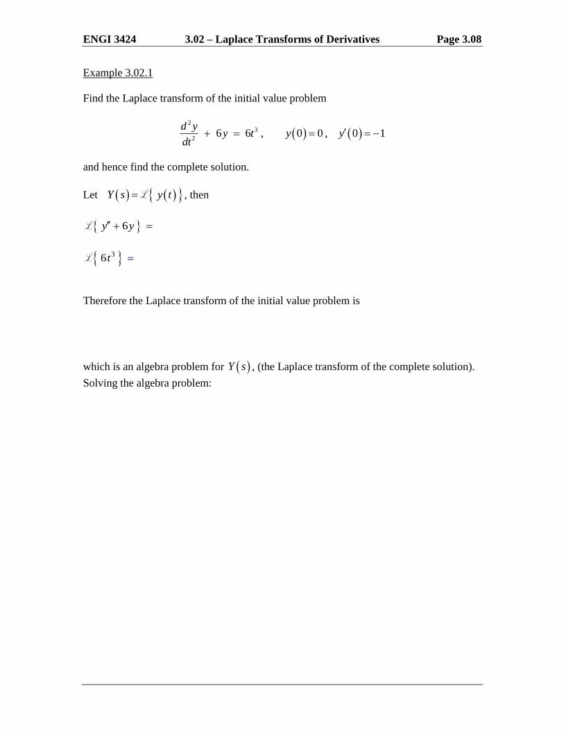
Example 3.02.1
Find the Laplace transform of the initial value problem
2
3
26 6 , 0 0 , 0 1
d yy t y y
dt
and hence find the complete solution.
Let Y s y t L , then
6y y L
36t L
Therefore the Laplace transform of the initial value problem is
which is an algebra problem for Y s , (the Laplace transform of the complete solution).
Solving the algebra problem:

ENGI 3424 3.03 – Review of Complex Numbers Page 3.09
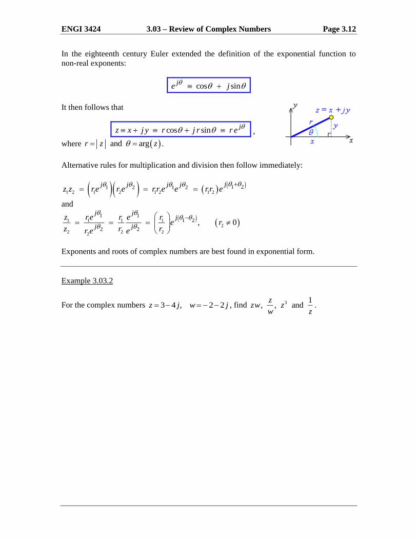
3.03 Review of Complex Numbers
Before proceeding further with Laplace transforms, some familiarity with complex
numbers is required. A very brief review of complex numbers is provided here.
The set of real numbers is closed under addition, subtraction, multiplication and (with
the exception of zero) division. However, the square root of any negative number is
not real. This generates the set of imaginary numbers, which are all real multiples of the
imaginary number 1j . For example: 49 49 1 49 1 7 j .
Imaginary and real numbers can be combined by addition to form the set of complex
numbers, which can be represented on an Argand diagram:
Example 3.03.1
Two complex numbers are defined by 3 2z j and 1 3w j :
The real parts of these numbers are Re 3z and Re 1w
The imaginary parts of these numbers are Im 2z and Im 3w
The sum (or difference) of any pair of complex numbers is calculated by taking the sum
(or difference) of the real parts and imaginary parts separately:

ENGI 3424 3.03 – Review of Complex Numbers Page 3.10
The real and imaginary parts of a complex number z x y j behave on the Argand
diagram very like the Cartesian x and y components of a vector x
y
v :
Also like vectors in 2, complex numbers can be expressed in terms of their magnitude
and direction.
The modulus (or “magnitude” or “amplitude”) of z x y j
(which is also the length of the vector x
y
v ) is 2 2z x y j x y
The argument (or “phase”) of z x y j
(which is also the angle that the vector x
y
v makes with the positive x axis) is ,
where tany
x . When Re 0z x , add or subtract radians from the inverse
tangent in order to be in the correct quadrant (2nd
or 3rd
, not 4th
or 1st).
The principal argument is usually taken to be in the range or 0 2 .
In Example 3.03.1,

ENGI 3424 3.03 – Review of Complex Numbers Page 3.11
Multiplication and Division of Complex Numbers
Example 3.03.1 (continued)
3 2 1 3zw j j
It is generally true that
zw z w and arg arg argzw z w
Also, for division (where the divisor is not zero),
zz
w w and arg arg arg
zz w
w
The argument of the product or quotient may need to be adjusted by the addition or
subtraction of 2 in order to bring it back inside the range of the principal argument.
ENGI 3424 3.03 – Review of Complex Numbers Page 3.12
In the eighteenth century Euler extended the definition of the exponential function to
non-real exponents:
cos sinj
e j
It then follows that
cos sinj
z x j y r j r r e
,
where and argr z z .
Alternative rules for multiplication and division then follow immediately:
1 2 1 2 1 2 1 21 21 2 1 2
jj j j jz z re r e rr e e rr e
and
1 1 1 1
2
2 2 22
1 11 2
2 2, 0
j jj
j j
z re r ree r
z r rr e e
Exponents and roots of complex numbers are best found in exponential form.
Example 3.03.2
For the complex numbers 3 4 , 2 2z j w j , find 3 1, , and
zzw z
w z.
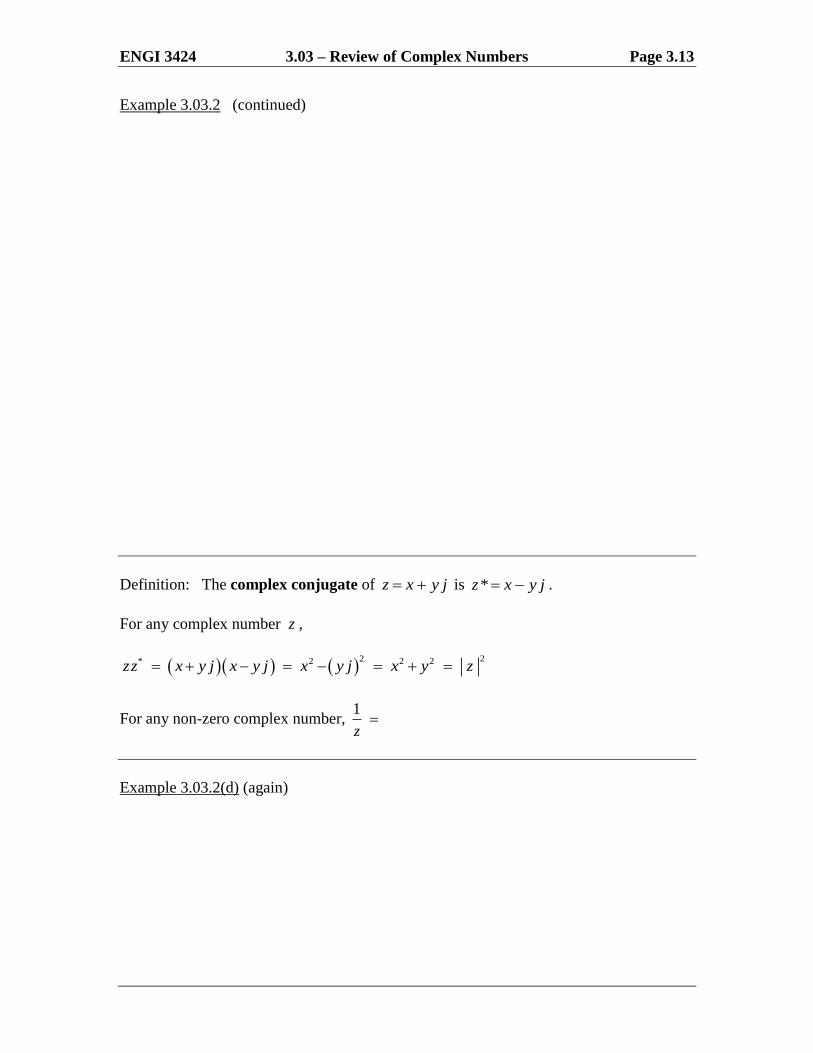
ENGI 3424 3.03 – Review of Complex Numbers Page 3.13
Example 3.03.2 (continued)
Definition: The complex conjugate of z x y j is *z x y j .
For any complex number z ,
22* 2 2 2zz x y j x y j x y j x y z
For any non-zero complex number, 1
z
Example 3.03.2(d) (again)

ENGI 3424 3.03 – Review of Complex Numbers Page 3.14
Example 3.03.3
Find all distinct cube roots of the real number 8.
The only real cube root of 8 is 2. However, there is a pair of non-real roots also.
Method 1
Let z be a cube root of 8, then 3 8z
Method 2
3 3
1/30 2 0 2 2 /3
8 2 , 2 2j n j n j n
z e n z e e
2 22cos 2 sin
3 3
n nz j
0 2cos0 2 sin0 2n z j
2 21 2cos 2 sin 1 3
3 3n z j j
2 21 2cos 2 sin 1 3
3 3n z j j
and these are the only three distinct values.
n = ..., –7, –4, 2, 5, 8, ... return the same value for z as n = –1.
n = ..., –6, –3, 3, 6, 9, ... return the same value for z as n = 0.
n = ..., –5, –2, 4, 7, 10, ... return the same value for z as n = +1.

ENGI 3424 3.03 – Review of Complex Numbers Page 3.15
Example 3.03.3 (continued)
On the Argand diagram the roots are equally spaced around a circle
of radius 2 centred on 0.
A similar graphical approach can be used to find the n distinct nth roots of any non-zero
complex number.

ENGI 3424 3.03 – Review of Complex Numbers Page 3.16
Example 3.03.4
On the Argand diagram sketch the locations of the five distinct fifth roots of the complex
number w. You may assume that the radius of the guide circle is 5 w .
Also note that cos sinj
e j
and
cos sin cos sinj
e j j
and

ENGI 3424 3.04 – First Shift Theorem, Cosine and Sine Page 3.17
3.04 First Shift Theorem, Transform of Exponential, Cosine and Sine Functions
ate f t L
The first shifting theorem then follows:
If , then atf t F s e f t F s a L L
Example 3.04.1
Find 3 5tt eL .
Example 3.04.2
Find ateL .

ENGI 3424 3.04 – First Shift Theorem, Cosine and Sine Page 3.18
Example 3.04.3
Find cos tL .
Example 3.04.4
Find sin tL .
It then follows that
1
2 2cos
st
s
L and
1
2 2
1 sin t
s
L
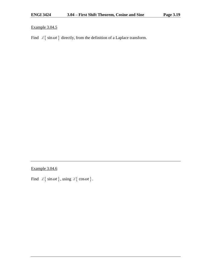
ENGI 3424 3.04 – First Shift Theorem, Cosine and Sine Page 3.19
Example 3.04.5
Find sin tL directly, from the definition of a Laplace transform.
Example 3.04.6
Find sin tL , using cos tL .

ENGI 3424 3.04 – First Shift Theorem, Cosine and Sine Page 3.20
Example 3.04.7
Find sinate tL .
Using the first shift theorem, we have, immediately,
Similarly,
2 2cosat s a
e ts a
L
Example 3.04.8
Find tan tL .
Example 3.04.9
Find sinh atL .
Similarly, 2 2cosh
sat
s a
L
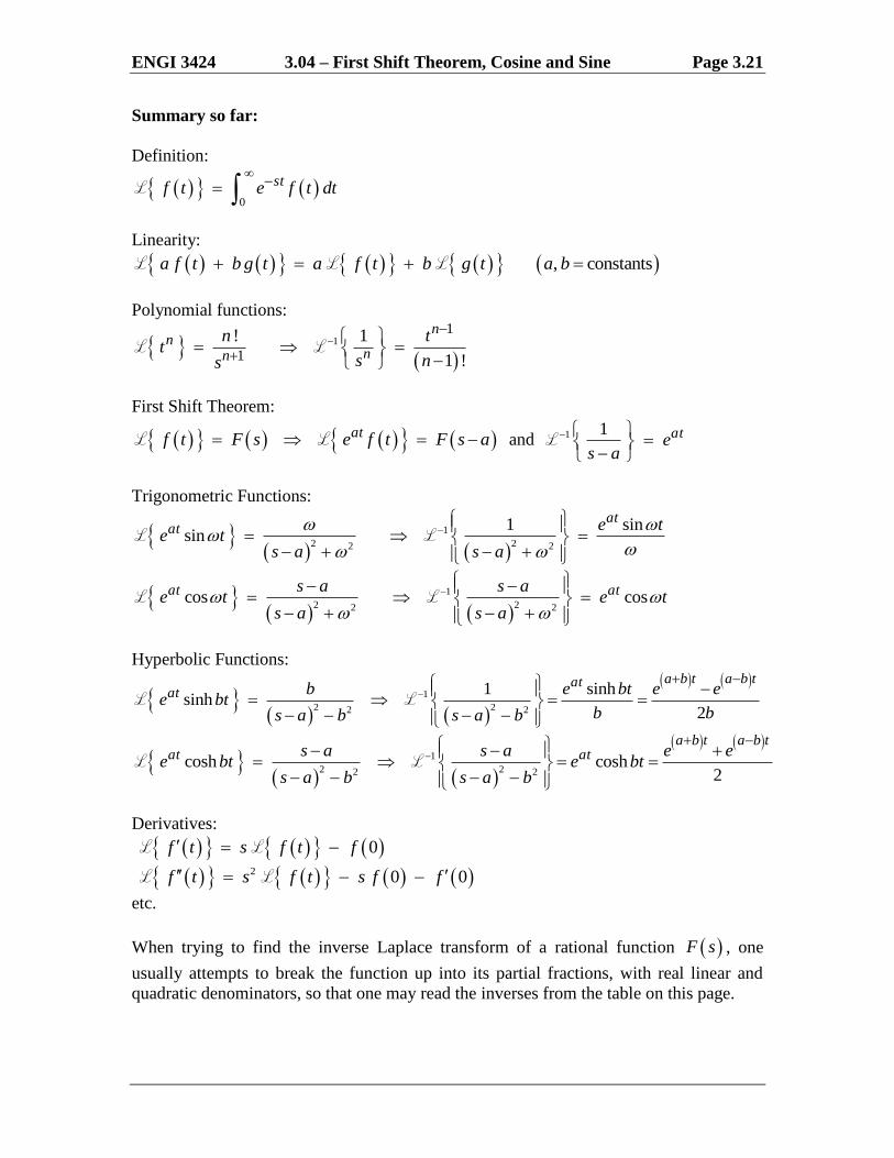
ENGI 3424 3.04 – First Shift Theorem, Cosine and Sine Page 3.21
Summary so far:
Definition:
0
stf t e f t dt
L
Linearity:
, constantsa f t b g t a f t b g t a b L L L
Polynomial functions:
11
1
! 1
1 !
nn
nn
n tt
s ns
L L
First Shift Theorem:
atf t F s e f t F s a L L and 1 1 ates a
L
Trigonometric Functions:
1
2 22 2
1 sinsin
atat e t
e ts a s a
L L
1
2 22 2cos cosat ats a s a
e t e ts a s a
L L
Hyperbolic Functions:
1
2 22 2
1 sinhsinh
2
a b t a b tatat b e bt e e
e btb bs a b s a b
L L
1
2 22 2cosh cosh
2
a b t a b tat ats a s a e e
e bt e bts a b s a b
L L
Derivatives:
0f t s f t f L L
2 0 0f t s f t s f f L L
etc.
When trying to find the inverse Laplace transform of a rational function F s , one
usually attempts to break the function up into its partial fractions, with real linear and
quadratic denominators, so that one may read the inverses from the table on this page.

ENGI 3424 3.05 – Applications to Initial Value Problems Page 3.22
3.05 Applications to Initial Value Problems
Example 3.05.1
Solve the initial value problem
5 6 0 , 0 1, 0 0y y y y y
Let Y s y t L .
y t L
y t L
Taking the Laplace transform of the entire initial value problem:
5 6 0y y y L L
Check 1:

ENGI 3424 3.05 – Applications to Initial Value Problems Page 3.23
Example 3.05.1 (continued)
Check 2:
Solution by Chapter 2 method:
5 6 0y y y
ENGI 3424 3.05 – Applications to Initial Value Problems Page 3.24
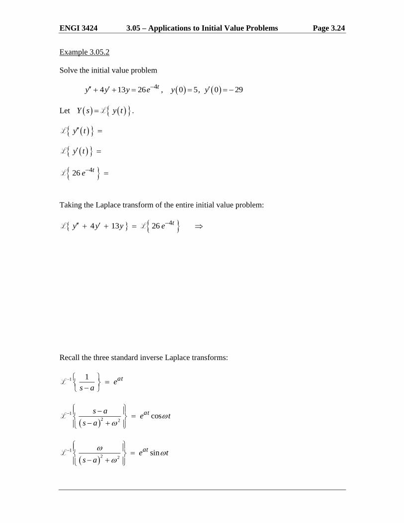
Example 3.05.2
Solve the initial value problem
44 13 26 , 0 5, 0 29ty y y e y y
Let Y s y t L .
y t L
y t L
426 te L
Taking the Laplace transform of the entire initial value problem:
44 13 26 ty y y e L L
Recall the three standard inverse Laplace transforms:
1 1 ates a
L
1
2 2cosats a
e ts a
L
1
2 2sinate t
s a
L

ENGI 3424 3.05 – Applications to Initial Value Problems Page 3.25
Example 3.05.2 (continued)
We need to express Y s in partial fractions and to complete the square in the quadratic
denominator.

ENGI 3424 3.05 – Applications to Initial Value Problems Page 3.26
Example 3.05.2 (by a Chapter 2 method)
44 13 26 , 0 5, 0 29ty y y e y y

ENGI 3424 3.06 – Laplace Transform of an Integral Page 3.27
3.06 Laplace Transform of an Integral
0
Let , thent
f t g d
Example 3.06.1
Find the function f t whose Laplace transform is 2 2
1F s
s s
.

ENGI 3424 3.06 – Laplace Transform of an Integral Page 3.28
Example 3.06.1 (Alternative solution, using partial fractions)
Example 3.06.2
Find the function f t whose Laplace transform is 2 2 2
1F s
s s
.
Alternative method, using partial fractions:

ENGI 3424 3.07 – Heaviside Function, Second Shift Theorem Page 3.29
3.07 Heaviside Function, Second Shift Theorem; Example for RC Circuit
The Heaviside function H t a (also known as the unit step function u t a ) is
defined by
00
1
t aH t a a
t a
The Laplace transform of the
Heaviside function is:
F s H t a L
If
0,
g t t af t
h t t a
then
ON OFF
f t g t h t g t H t a
[The function h t is “switched on” and g t is “switched off” at time t = a.]

ENGI 3424 3.07 – Heaviside Function, Second Shift Theorem Page 3.30
Example 3.07.1
Express the function
2 2
4 2
x xf x
x
in a single line definition.
Answer: f x
The Second Shift Theorem
The result of shifting the graph y f t (defined only for t > 0) a units to the right, is
the graph y f t a H t a :
The Laplace transform of the shifted function of t is:
0
stH t a f t a e H t a f t a dt
L
H t a f t a L
The second shift theorem (for a > 0) is
asH t a f t a e f t L L
ENGI 3424 3.07 – Heaviside Function, Second Shift Theorem Page 3.31
Another way to express the second shift theorem is:
1 1 asF s f t e F s H t a f t a L L
Example 3.07.2
Find 34 4H t t L .
34 4H t t L
Example 3.07.3
Find the function whose Laplace transform is 2
5
4
se
s
.

ENGI 3424 3.07 – Heaviside Function, Second Shift Theorem Page 3.32
Example 3.07.4
In the RC circuit shown here, there is no
charge on the capacitor and no current
flowing at the time t = 0.
The input voltage Ein is a constant Eo
during the time 1 2t t t and is zero at all
other times.
Find the output voltage Eout for this circuit.
Initial conditions:
q(0) = i(0) = 0 Note:dq
idt
o 1 2
in0 otherwise
E t t tE
inE
Equating voltage drops around the circuit with inE :
Let Q s q t L . Taking the Laplace transform of this initial value problem:

ENGI 3424 3.07 – Heaviside Function, Second Shift Theorem Page 3.33
Example 3.07.4 (continued)
Graph of the output voltage against time:

ENGI 3424 3.07 – Heaviside Function, Second Shift Theorem Page 3.34
Example 3.07.5
Find the complete solution of the initial value problem
2
2
0 0 34 ; 0 0 0 .
3
td yy f t y y
t td t
Let Y s y t L

ENGI 3424 3.07 – Heaviside Function, Second Shift Theorem Page 3.35
Example 3.07.5 (continued)

ENGI 3424 3.08 – Dirac Delta Function Page 3.36
3.08 Dirac Delta Function, Example for Mass-Spring System
1
Let
0 otherwise
a t af t
0
Area under Area of
graph rectangle
11f t dt
Also
f t
Define the Dirac delta function to be
0
limt a f t
then
f t L
t a L
Therefore for 0a
and
Also, for 0a , the total area under the graph is 1 (even in the limit as 0+), so
0
1t a dt
ENGI 3424 3.08 – Dirac Delta Function Page 3.37
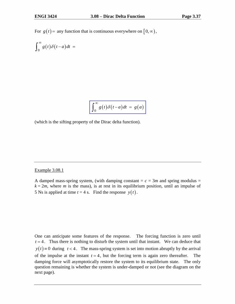
For g t any function that is continuous everywhere on 0, ,
0
g t t a dt
0
g t t a dt g a
(which is the sifting property of the Dirac delta function).
Example 3.08.1
A damped mass-spring system, (with damping constant = c = 3m and spring modulus =
k = 2m, where m is the mass), is at rest in its equilibrium position, until an impulse of
5 Ns is applied at time t = 4 s. Find the response y t .
One can anticipate some features of the response. The forcing function is zero until
4t . Thus there is nothing to disturb the system until that instant. We can deduce that
0y t during 4t . The mass-spring system is set into motion abruptly by the arrival
of the impulse at the instant 4t , but the forcing term is again zero thereafter. The
damping force will asymptotically restore the system to its equilibrium state. The only
question remaining is whether the system is under-damped or not (see the diagram on the
next page).

ENGI 3424 3.08 – Dirac Delta Function Page 3.38
Example 3.08.1 (continued)
Anticipated response:
The auxiliary equation is 2 3 2 0 . The discriminant is
Solution, using Laplace transforms:
3 2 5 4y y y t
0 0 0y y
Let Y s y t L

ENGI 3424 3.08 – Dirac Delta Function Page 3.39
Example 3.08.1 (continued)
From the first shift theorem: 1 1 ates a
L
The second shift theorem states:
1 1 asF s f t e F s f t a H t a L L
Therefore
or, equivalently,

ENGI 3424 3.09 – Periodic Functions Page 3.40
3.09 Laplace Transform of Periodic Functions; Square and Sawtooth Waves [only if time permits]
If the constant 0p and f t p f t for all 0t , then
f t is a periodic function of t, with period p.
Example of a periodic function (with one finite discontinuity in each period):
Define a new set of functions ng t , each of which captures only a single period of f t :
1
0 otherwisen
f t np t n pg t
Then 0n
nf t g t
0
Let n
stn nG s g t e g t dt
L
1 1
0 0n p n p
st stn
n p n pe g t dt e f t dt
Let F s f t L , then

ENGI 3424 3.09 – Periodic Functions Page 3.41
Therefore, for a periodic function f t with fundamental period p,
0
1
1
pst
s pf t e f t dte
L
Example 3.09.1
Use the formula above to verify the Laplace transform of sinf t t .

ENGI 3424 3.09 – Periodic Functions Page 3.42
Example 3.09.2 The Square Wave
The square wave is periodic, with fundamental period 2p a .
In the “zeroth” period 0 2t a ,
0
1 0
1 2
t af t g t
a t a
The Laplace transform F s of the square wave f t then follows.

ENGI 3424 3.09 – Periodic Functions Page 3.43
Example 3.09.3 The Saw-tooth Wave
The saw-tooth wave is periodic, with fundamental period p a .
In the “zeroth” period 0 t a ,
0
btf t g t
a
The Laplace transform F s of the saw-tooth wave f t then follows.

ENGI 3424 3.09 – Periodic Functions Page 3.44
Example 3.09.4
Find the function f t whose Laplace transform is 2
1tanh
2
asF s
s
(where a is a constant).

ENGI 3424 3.10 – Derivative of a Laplace Transform Page 3.45
3.10 Derivative of a Laplace Transform [only if time permits]
Example 3.10.1
Find cosF s t t L .
Method via an ODE:
Let cosf t t t
Then f t
and f t
Also 0f
0f
Taking the Laplace transform of this initial value problem,
0 0
st stdF s f t e f t dt F s e f t dt
ds
L
Using Leibnitz differentiation of an integral:
00
0 0 st stF s e f t dt e t f t dts
Therefore
d
f t t f tds
L L 1 1F s t F s L L
ENGI 3424 3.10 – Derivative of a Laplace Transform Page 3.46
Example 3.10.1 (again)
Find cosF s t t L .
Method via the derivative of a transform:
Let cosg t t
Example 3.10.2
Find sinF s t t L .

ENGI 3424 3.11 – Convolution Page 3.47
3.11 Convolution; Integro-Differential Equations; Circuit Example
If f t F sL
and g t G sL
then the convolution of f t and g t is denoted by f g t , is defined by
0
t
f g t f g t d
and the Laplace transform of the convolution of two functions is the product of the
separate Laplace transforms:
f g t F s G s L
An equivalent identity is
1 1 1F s G s F s G s L L L
Convolution is commutative:
0 0
t t
g f f t g d f g t d f g
Example 3.11.1
Find the inverse Laplace transform of 2 2 2
1.R s
s s

ENGI 3424 3.11 – Convolution Page 3.48
Example 3.11.1 (continued)
Note:
This inverse transform can also be found using partial fractions or the division of another
Laplace transform by s. Both of these alternatives are in example 3.06.2.

ENGI 3424 3.11 – Convolution Page 3.49
Example 3.11.2
Find
1
22 2
1.
s
L
The alternative methods that were available in example 3.11.1 are not available here.
The only obvious way to proceed is via convolution.
22 2
1Let R s
s

ENGI 3424 3.11 – Convolution Page 3.50
Some More Identities involving Convolution [only if time permits]
1 y
ENGI 3424 3.11 – Convolution Page 3.51
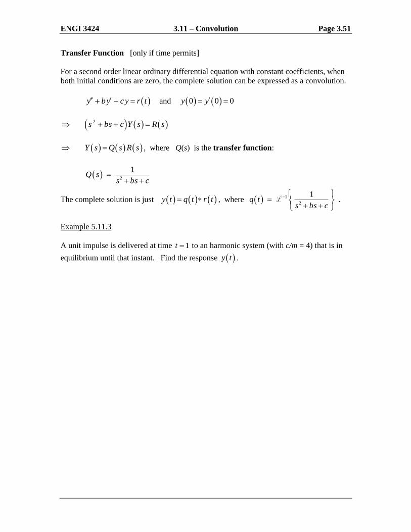
Transfer Function [only if time permits]
For a second order linear ordinary differential equation with constant coefficients, when
both initial conditions are zero, the complete solution can be expressed as a convolution.
y by cy r t and 0 0 0y y
2s bs c Y s R s
Y s Q s R s , where Q(s) is the transfer function:
2
1Q s
s bs c
The complete solution is just y t q t r t , where 1
2
1.q t
s bs c
L
Example 5.11.3
A unit impulse is delivered at time 1t to an harmonic system (with c/m = 4) that is in
equilibrium until that instant. Find the response y t .
ENGI 3424 3.11 – Convolution Page 3.52
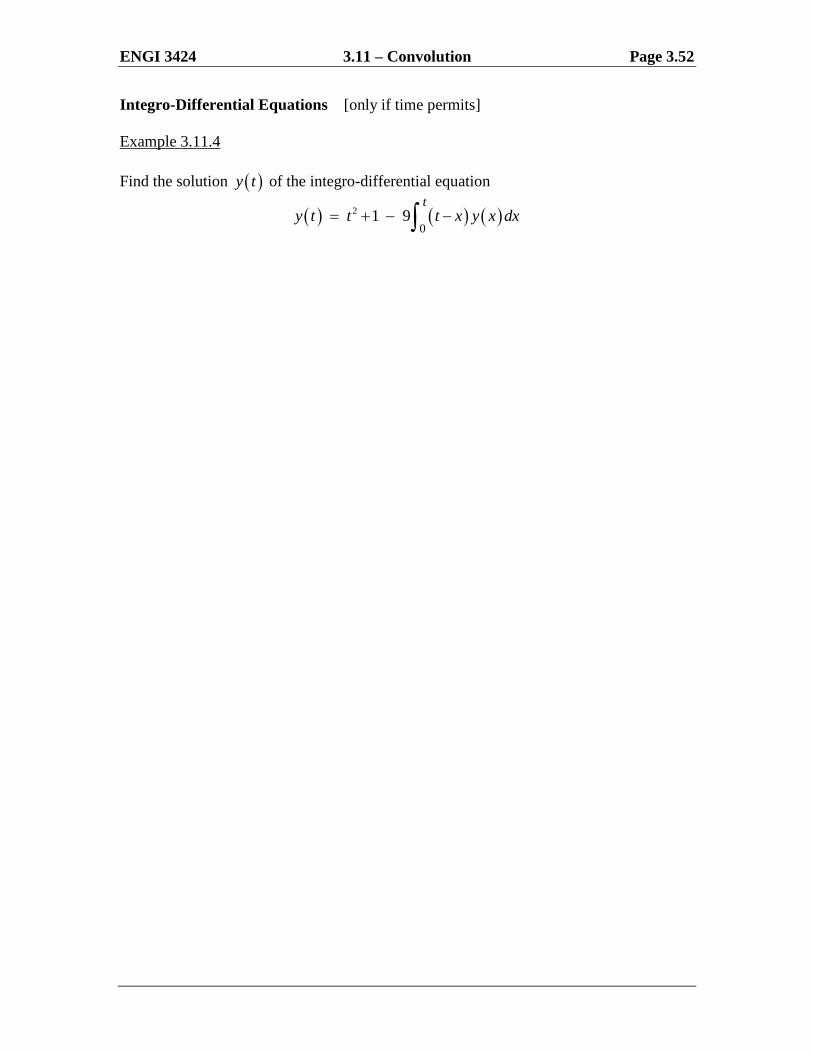
Integro-Differential Equations [only if time permits]
Example 3.11.4
Find the solution y t of the integro-differential equation
2
01 9
ty t t t x y x dx

ENGI 3424 3.11 – Convolution Page 3.53
Example 3.11.5 [only if time permits]
Solve the system of simultaneous integral equations
1 1 2
2 2 1 2
0
0 0
4 12 1
2 2
t
t t
i i i d
i i d i i d
1 1 2 2Let , .I s i t I s i t L L
Taking the Laplace transform of the entire system of integral equations,

ENGI 3424 3.11 – Convolution Page 3.54
Example 3.11.5 (continued)
These are the currents in the circuit
with initial conditions 1 2
14
0 , 0 0i i .
END OF CHAPTER 3


![Engi 5035fa05[Assignment6solution]](https://img.dokumen.tips/doc/110x75/563db840550346aa9a91fabf/engi-5035fa05assignment6solution.jpg)


