Embed Size (px)
Citation preview

Reference Manual on
Energy Recovery and Reuse
(Under Singapore Certified Energy Manager Programme)
By
Gade Pandu Rangaiah
(Department of Chemical and Biomolecular Engineering,
National University of Singapore)
and
Andrew Morrison
(September 2019)

ii
Preface
Energy Recovery and Reuse (ERR) is essential for improving not only energy efficiency but
also economic performance of many manufacturing industries and building facilities. A
course/module on ERR is one of the electives for certification under the Singapore Certified
Energy Manager (SCEM) Programme. The purpose of this programme is to equip facility
managers, engineers and others, who wish to become energy managers and professionals,
with the required technical skills and competencies to manage and improve energy-consuming
units and processes in their organisations. Full details on the SCEM programme are readily
available on the Internet.1
The major topic of ERR is recovery and reuse of thermal energy (or heat) using pinch analysis,
which has been successfully used in various industries and facilities. Other topics in ERR are
recovery of heat at low temperatures and other energy recovery techniques and technologies.
This reference manual on ERR is prepared under a project of the National Environment
Agency (NEA), Singapore. We, the authors of this reference manual, have been co-teaching
the 3-day ERR course/module for a number of years. Moreover, we have many years of
professional experience in teaching, research and/or consultancy projects in ERR and related
fields.
This reference manual on ERR has 12 chapters. The first two chapters, namely, Introduction
(Chapter 1) and Heat Exchanger Types and Principles (Chapter 2) cover the background
necessary for the remaining chapters. Chapters 3 to 8 are on basic principles and systematic
procedures in pinch analysis for heat recovery and reuse; for easy learning, each of these
chapters is focused on only one or two aspects of pinch analysis. Chapters 9 and 10 introduce
an approach to improving the energy efficiency of the overall site, including the site utility
system and the recovery of low grade heat. Chapter 11 introduces other energy recovery
techniques and technologies for common equipment items before Chapter 12 provides a case
study on how to systematically implement an energy improvement programme and how such
programmes have been successfully applied in the past.
In all chapters of this reference manual, principles and procedures are described and
illustrated with suitable examples. Many exercises are given at the end of each chapter for
readers to try and solve. These exercises include questions to test the understanding of
concepts and principles covered in the chapter. Readers can gain deeper understanding of
1 https://www.ies.org.sg/Registries/Singapore%20Certified%20Energy%20Manager%20Registry.

iii
concepts, principles and procedures in ERR by solving the exercises by themselves. The
material (i.e. description, illustrations and exercises) in each chapter have been thoughtfully
prepared based on our extensive experience in teaching ERR (e.g. considering questions
posed by participants). Many diagrams are prepared in colour to facilitate learning.
The learning outcomes of this reference manual on ERR are:
1. Describe pinch analysis and its methodologies, benefits and applications
2. Apply pinch analysis methods to find targets for heat exchanger networks
3. Apply pinch analysis methodology to design and evolve heat exchanger networks
4. Discuss other energy recovery techniques for chemical and process industries
5. Analyse and improve energy efficiency of chemical, thermal and related processes
To achieve the above learning outcomes and to master the principles and procedures in ERR,
motivated readers should study each chapter carefully, check the calculations in the solved
examples and then attempt all exercises at the end of the chapter. Many chapters in this
reference manual require concepts and principles learnt in one or more earlier chapters.
Hence, for effective learning, readers should read the chapters following the sequence in this
reference manual.
This reference manual should be useful to engineers and managers, who are interested in
energy recovery and reuse by pinch analysis and other technologies. It is also beneficial to
those taking the ERR module under the SCEM programme. Despite numerous hours required,
we enjoyed preparing the material including numerous diagrams in this reference manual on
ERR, and are pleased and satisfied with the final version. We tried our best to avoid
typographical errors, and we welcome comments for enhancing this reference manual
(including compliments and typos) from readers. These can be sent to the first author at
We are thankful to all those who have helped us in preparing this reference manual on ERR.
In particular, we thank Andy Ong of IES for his coordination and understanding, and also the
anonymous reviewer(s) of this reference manual. Finally, we are grateful to our respective
families for their deep affection and unwavering support.
Gade Pandu Rangaiah and Andrew Morrison

iv
Table of Contents
Page
Preface ii
Acronyms and Notation viii
Chapter 1 – Introduction
1.1 Overview 1
1.2 Energy Recovery, Reuse and Efficiency 1
1.3 Heat Exchanger Networks 3
1.4 Pinch Analysis 8
1.5 Scope and Outline of Chapters 10
1.6 Learning Outcomes of this Reference Manual 12
1.7 Books and References for Additional Learning 12
1.8 References 13
1.9 Exercises 14
Chapter 2 – Heat Exchangers: Types and Basic Principles
2.1 Overview 15
2.2 Heat Exchangers and their types 15
2.3 Heat Exchanger Configurations 19
2.4 Heat Exchanger Design Equations 20
2.5 Heat Transfer Coefficients 25
2.6 Heat Transfer Enhancements 27
2.7 Heat Exchanger Costs 28
2.8 Summary 30
2.9 References 31
2.10 Exercises 32
Chapter 3 – Pinch Analysis: Stream Data and Utility Targets
3.1 Overview 34
3.2 Stream Data for Heat Integration 35
3.3 Guidelines for Choosing Streams 39
3.4 Example and Energy Balance 42

v
3.5 Composite Curves and Minimum Utilities 43
3.6 Problem Table Procedure for Finding Minimum Utilities 52
3.7 Pinch and its Significance 57
3.8 Summary 61
3.9 References 61
3.10 Exercises 62
Chapter 4 – Pinch Analysis: Number of Units, Heat Transfer Area
and Supertargeting
4.1 Overview 67
4.2 Target on Number of Units 68
4.3 Total Heat Transfer Area 73
4.4 Supertargeting for Finding the Optimum (T)min 78
4.5 Summary 80
4.6 References 81
4.7 Exercises 81
Chapter 5 – Pinch Analysis: Heat Exchanger Network Design
5.1 Overview 83
5.2 Grid Representation of HEN 83
5.3 Conventional HEN Design 86
5.4 Pinch Design of HEN 88
5.5 Summary 95
5.6 References 95
5.7 Exercises 96
Chapter 6 – Pinch Analysis: Grand Composite Curve, Threshold
Problems and Multiple Utilities
6.1 Overview 98
6.2 Grand Composite Curve 99
6.3 Threshold Problems 100
6.4 HEN Design for Threshold Problems 104
6.5 Multiple Utilities 110
6.6 HEN Design for Multiple Utilities 117
6.7 Summary 121

vi
6.8 References 122
6.9 Exercises 122
Chapter 7 – Pinch Analysis: Design via Stream Splitting and Cyclic
Matching
7.1 Overview 125
7.2 Stream Splitting and Number Criterion 126
7.3 Stream Splitting for Satisfying MCp Criterion 129
7.4 Algorithm for Stream Splitting 134
7.5 Cyclic Matching 135
7.6 Design Away from the Pinch 139
7.7 Summary 139
7.8 References 140
7.9 Exercises 140
Chapter 8 – Pinch Analysis: Heat Exchanger Network Evolution
8.1 Overview 142
8.2 Purpose and Potential of HEN Evolution 143
8.3 Loops in HEN 144
8.4 Loop Breaking 146
8.5 Violation and Restoration of (∆T) 147
8.6 Another Example of Loop Breaking and Restoration of (∆T) 151
8.7 HEN Evolution in Other Situations 152
8.8 HEN for MER versus Evolved HEN 157
8.9 Summary 158
8.10 References 158
8.11 Exercises 159
Chapter 9 – Introduction to Low Grade Heat Recovery
9.1 Overview 161
9.2 Organic Rankine Cycle 162
9.3 Absorption Refrigeration 163
9.4 Desalination 166
9.5 Technology Selection 173
9.6 Summary 178
9.7 References 178

vii
9.8 Exercises 179
Chapter 10 – Site Wide Planning for Energy Improvement Strategies
10.1 Overview 180
10.2 Site Source/Sink Profiles 181
10.3 Analysing the Utility System 188
10.4 Total Site Summary 195
10.5 Total Area Analysis 196
10.6 Total Site Analysis for Low Grade Heat Recovery 197
10.7 Summary 203
10.8 References 203
10.9 Exercises 204
Chapter 11 – Other Energy Recovery Techniques and Technologies
11.1 Overview 207
11.2 Heat Exchangers 208
11.3 Power Recovery 209
11.4 Heat Pumps 212
11.5 Rotating Equipment Efficiency 217
11.6 Summary 224
11.7 References 225
11.8 Exercises 225
Chapter 12 – Industrial Applications
12.1 Overview 227
12.2 Case Study 228
12.3 Summary 237
12.4 References 237
12.5 Exercises 238

viii
Acronyms and Notation
Acronyms
BEP Best Efficiency Point
BFW Boiler Feed Water
CC Capital Cost (S$)
COP Coefficient of Performance
CS Cold Stream
CU Cold Utility (kW)
CW Cooling Water
GCC Grand Composite Curve
EDR Electrodialysis Reversal
HE Heat Exchanger
HEN Heat Exchanger Network
HP High Pressure
HPRT Hydraulic Pressure Recovery Turbine
HPS High Pressure Steam
HS Hot Stream
HU Hot Utility (kW)
IP Intermediate Pressure
IPS Intermediate (between medium and low) Pressure Steam
LGH Low Grade Heat
LNG Liquefied Natural Gas
LP Low Pressure
LPS Low Pressure Steam
MED Multi Effect Distillation
MER Maximum Energy Recovery
MP Medium Pressure
MPS Medium Pressure Steam
MSF Multi-Stage Flash
MVC Mechanical Vapour Compression
OC Operating Cost (S$/year)
ORC Organic Rankine Cycle

ix
PFD Process Flow Diagram
PTA Purified terephthalic acid
SSSP Site Source Sink Profile
RO Reverse Osmosis
TAC Total Annual Cost (S$/year)
TVC Thermal Vapour Compression
VFD Variable Frequency Drive
VHP Very High Pressure
VSD Variable Speed Drive
VVLP Very Very Low Pressure
Notation
A Heat transfer area of a heat exchanger (m2)
Cp Heat capacity (specific heat) of a stream (kJ/kg.K or kJ/kg.oC)
H Enthalpy of a stream (kW)
∆H Enthalpy change (kW)
h Film heat transfer coefficient of a stream (kW/m2.K or kW/m2.oC)
hF Fouling coefficient of a stream (kW/m2.K or kW/m2.oC)
kW Kilowatt
kWh Kilowatt-hour
M Mass flow rate of a stream (kg/s)
MCp Product of mass flow rate and heat capacity of a stream (kW/K or kW/oC)
MW Megawatt
MWh Megawatt-hour
MWhTH Megawatt-hour (of thermal energy)
nc Number of cold streams
nh Number of hot streams
ns Number of subsets for finding number of units in heat exchanger network
nu Number of utility streams
Q Heat duty of (i.e. heat transferred from one stream to another in) a heat
exchanger (kW)
T Temperature (oC or K)
u Number of units (i.e. heat exchangers, heaters and coolers in total)

x
U Overall heat transfer coefficient of a heat exchanger (kW/m2.K or
kW/m2.oC)
∆T Temperature difference (oC or K)
W Work (provided as power)
Subscripts
c Refers to cold stream
h Refers to a hot stream
i Refers to inlet or inner condition(s)
LM Log mean
MER Maximum energy recovery
min Minimum
o Refers to outlet or outer condition(s)
S Refers to supply or initial value
T Refers to target or final value
p Subscript in heat capacity (Cp)

1
Chapter 1
Introduction
By
Gade Pandu Rangaiah and Andrew Morrison
1.1 Overview
Energy recovery and reuse is essential in industries and buildings for both economic and
environmental benefits. In this introduction chapter, the potential for energy recovery and
reuse in process and related industries is described. Then, heat exchanger networks and
pinch analysis, which are important for energy recovery and reuse, are introduced. Next, the
content and learning outcomes of this reference manual are outlined. Finally, two books for
additional learning are briefly described.
The learning outcomes of this introduction chapter are as follows:
1. Describe energy recovery and reuse being achieved in process and related industries
2. Describe heat exchangers and heat integration
3. Name available technologies for energy recovery and reuse
4. Identify potential for energy recovery and reuse in learner’s workplace
1.2 Energy Recovery, Reuse and Efficiency
New plants in chemical and related process industries are being designed and set-up to meet
the market demand for their products. Perhaps, these new plants are better designed with the
latest technologies for efficient operation. On the other hand, existing plants in process and
related industries were designed and built in the past. They continue to operate with some
modifications for one reason or other. Is it possible to improve the energy efficiency of these
existing plants by energy recovery and reuse? The answer is yes because of changing
economic and environmental considerations as well as technological developments.
According to the website of Natural Resources Canada2, which oversees natural resources
and energy in the country, the potential for energy savings through process/heat integration is
10% or more in various industries such as oil refining, petrochemicals, chemicals, and food &
2 http://www.nrcan.gc.ca/energy/efficiency/industry/processes/systems-optimization/5495 (accessed
in August 2018)

2
beverages. It also suggests optimising system operation through data mining, and improving
energy efficiency through research and development in waste heat recovery and fault
diagnosis. Indeed, energy recovery and reuse techniques are widely employed in process
industries in Singapore to improve energy efficiency, as can be seen from the following
examples.
ExxonMobil uses their proprietary Global Energy Management System (GEMS) in improving
energy efficiency of their manufacturing operations.3 According to a report in The Business
Times in 2016, ExxonMobil improved energy efficiency of their Singapore refinery and
ethylene cracker by more than 17% over 12 years to the year 2014. In one of their projects4,
pinch analysis for heat integration (which is the major topic in this reference manual) was used
to identify opportunities for improving energy efficiency and to replace three existing shell-and-
tube exchangers by two welded plate heat exchangers; this project achieved annual fuel
savings of 8.7%.
GlaxoSmithKline is a well-known pharmaceutical company and has been operating its plants
in Singapore for more than 35 years. The company’s Jurong waste heat recovery project5
resulted in the generation of sufficient steam to reduce fresh fuel needed, as well as chilled
water, using absorption chiller, which lowered the cooling load on existing mechanical chillers.
All these improved the energy efficiency of the plant.
Nestlé Singapore Pte Ltd retrofitted their multi-effect evaporator with a thermo vapour re-
compressor (TVR)6; this addition permitted re-use of the compressed vapour at a higher
temperature, thus reducing the amount of fresh steam required for concentrating malt extract
and improving energy efficiency of the unit. In general, Nestlé’s target is to achieve energy
savings of 2% year-on-year.7
3 http://www.exxonmobil.com.sg/en-sg/environment/energy-efficiency/reducing-emissions/mitigating-
greehouse-gas-emissions-in-our-operations (accessed in August 2018)
4 https://www.nea.gov.sg/media/releases/news/index/winners-from-diverse-organisations-recognised-
for-reducing-energy-use (accessed in August 2018)
5 http://www.icheme.org/media_centre/news/2016/national-university-of-singapore-scoop-three-
trophies-at-chemical-engineering-awards.aspx#.WUo4IeuGOpo (accessed in August 2018)
6 https://www.nea.gov.sg/media/releases/news/index/energy-efficiency-achievements-recognised-at-
energy-efficiency-national-partnership-awards-2015 (accessed in August 2018)
7 https://www.nea.gov.sg/docs/default-source/media-files/news-releases-docs/eenp---annex.pdf
(accessed in August 2018)

3
The above applications and others available through the links at NEA’s Energy Efficiency
National Partnership webpage8, show the potential of recovering and reusing energy to
improve energy efficiency of existing plants. On average, annual improvements in the energy
efficiency of process and related industries may be modest at about 2% but this can be
significant in terms of both cost savings and reduction in CO2 emissions because of the large
amount of energy/fuel used in these industries. This is similar to improving the energy
efficiency of engines in motor vehicles by a small percentage, which translates to significant
benefits to both producers and consumers because of the millions of vehicles that are sold
and used daily.
In short, drivers for energy efficiency improvement projects are both economic benefits and
reduction in environmental impact, which in turn benefit society and lead to sustainable
industries. We are confident and happy that this reference manual will help learners to
contribute to energy efficiency improvement efforts and sustainability of their businesses and
industries.
1.3 Heat Exchanger Networks
A heat exchanger is the equipment for transferring heat (i.e. thermal energy) from a hot stream
to a cold stream, usually without mixing the two streams involved. Heat exchangers are
present in industries, offices and homes. For example, split air conditioners have typically two
heat exchangers; one is in the room unit for heat transfer from the warm air in the room to the
cold refrigerant circulating in the air conditioner, while the other is in the outdoor (condenser)
unit for heat transfer from compressed refrigerant at a higher temperature to ambient air. Heat
transfer occurs during cooking on a stove from the flame to the food in the container. Many
types of heat exchangers are used in process and related industries, and common types of
exchangers are outlined in Chapter 2 of this reference manual.
Consider a cold stream (e.g. inlet stream to a processing unit) that has to be heated from 30oC
to 125oC, and its flow rate (M) and heat capacity (Cp, also known as specific heat) are 16 kg/s
and 4 kJ/kg.K9, respectively. One possibility for this heating is the use of steam, which is the
common utility in process and related industries. In this case, the heat exchanger is referred
to as a heater, as shown in Figure 1.1. Thermal energy needed for this heating is given by:
8 http://www.e2singapore.gov.sg/Programmes/Energy_Efficiency_National_Partnership/
EENP_Awards.aspx (accessed in August 2018) 9 Since temperature change of 1oC is equal to temperature difference of 1 K, heat capacity has the
same value with dimensions of kJ/kg.oC or kJ/kg.K.

4
Q = M × Cp × ∆T = 16 (kg
s) × 4 (
kJ
kg.K) × (125 − 30) = 6080 kW (1.1)
This value is referred to as the heat duty or simply duty of the heater.
Steam entering the heater is assumed to be saturated (although it may be slightly superheated
in practice, in order to avoid condensation in the supply pipeline). It condenses in the heater,
thus releasing the latent heat, which is transferred to the cold stream for its heating. The
condensate is assumed to leave the heater as saturated liquid (i.e. at the boiling point
corresponding to the steam pressure, and no sub-cooling to a lower temperature). In effect,
energy transferred to the cold stream is just the latent heat of condensation, whose value
depends on steam temperature/pressure. Assuming the latent heat of steam is 2000 kJ/kg,
steam required to supply 6080 kW of duty is
Steam required = 6080 kW
2000 kJ/kg= 3.04
kg
s or 10.9
t
h (1.2)
Assuming cost of steam10 is S$ 25/t and 8300 h of operation, annual cost of steam for heating
the process stream from 30oC to 125oC is S$ 10.9 x 8300 x 25 = S$ 2,261,750. Obviously,
this is substantial and provides a strong incentive to reduce steam required.
Figure 1.1: Heater for heating a cold stream using steam (left plot) and cooler for cooling a
hot stream using cooling water (right plot)
Plants may have some hot streams to be cooled as part of process requirements, for sending
to storage or for discharge as wastewater. Assume that there is a hot stream to be cooled
from 115oC to 40oC, its flow rate is 20 kg/s and its heat capacity is 3.8 kJ/kg.K (right plot in
Figure 1.1). This requires removal of the following amount of energy:
Q = 20 (kg
s) × 3.8 (
kJ
kg.K) × (115 − 40) = 5700 kW (1.3)
Cooling water is often used for removing energy from process streams. Assume cooling water
is available at 30oC, and it can be heated up to 45oC, which is typical in Singapore. Taking
10 It is important to note that costs vary from one plant to another, and also with time. Values used in
this reference manual are for illustrating the procedures and calculations. For any application in
learner’s company, relevant costs must be used and not the costs used in this reference manual.

5
heat capacity of cooling water to be 4.2 kJ/kg.K, the mass flow rate of cooling water (MCW)
required is given by the following energy balance:
Q = 5700 = MCW × 4.2kJ
kg.K (45 − 30) (1.4a)
Hence, MCW = 5700
4.2×15= 90.5
kg
s= 325.7
t
h (1.4b)
Assuming the cost of cooling water is S$ 0.08/t and 8300 h of operation, annual cost of cooling
water for cooling the process stream from 115oC to 40oC is S$ 325.7 x 8300 x 0.08 = S$
216,265. Comparing this with the annual cost of steam, it is clear that annual cost of water is
significantly less than that of steam. This does not mean that minimising cooling water usage
is not important.
Is it possible to recover thermal energy from the hot stream and reuse it for heating the cold
stream? Comparing temperatures of hot and cold streams in Figure 1.1, this is possible. As
shown in Figure 1.2, some thermal energy from the hot stream is transferred to heating the
cold stream to some extent in the heat exchanger. This is the central idea of heat integration,
which lowers both steam and cooling water required, and consequently reduce the annual
operating cost. However, the number of equipment (now 3 units, namely, heater, heat
exchanger and cooler) and capital cost for them may increase. In effect, there is trade-off
between capital and operating costs, which is the case in many practical situations.
Figure 1.2: Central idea of heat integration showing heat transfer from the hot stream to the
cold stream in a heat exchanger, before using cooling water and steam, respectively
Recall that heat available from cooling the hot stream is 5700 kW, and the heat required for
heating the cold stream is 6080 kW. Is it possible to use all of 5700 kW for heating the cold
stream? Assuming this is possible, the hot stream will be cooled to the final temperature of
40oC without the need of cooling water, and the outlet temperature of the cold stream entering
the exchanger at 30oC is given by the energy balance:
Q = 16 (kg
s) × 4 (
kJ
kg.K) × (T − 30) = 5700 (1.5)

6
Solving this equation, T = 119.1oC. This is higher than hot stream inlet temperature of 115oC,
which is not possible in the heat exchanger since heat transfer can only occur from a source
at a higher temperature to a lower temperature sink (unless additional energy is used as in air
conditioning).
Further, to avoid large equipment and to cater for variations during operation, there should be
certain minimum temperature difference, (∆T)min (e.g. 10oC) between hot and cold streams for
heat transfer. This difference between hot and cold stream temperatures is the temperature
driving force for heat transfer in a heat exchanger, and it is important for design of heat
exchangers and also heat exchanger networks by pinch analysis. It is different from the
temperature change of a stream, say, from 115oC to 40oC. This is the meaning and distinction
of the two phrases: ‘temperature difference’ and ‘temperature change’ throughout this
reference manual.
Thus, not all heat available from cooling the hot stream can be reused for heating the cold
stream. Then, how much of it can be used? This can be found by assuming that the cold
stream will be heated to 105oC (= 115 – 10) to ensure (∆T)min of 10oC at the right side (hot
end) of the heat exchanger, as shown in Figure 1.3. Heat recovered from the hot stream and
reused for the cold stream as well as temperature of the hot stream leaving the exchanger can
be calculated. These values and heat duties of heater, heat exchanger and cooler are shown
in Figure 1.3. Verify the results shown in this figure using equations similar to Equations 1.1
to 1.5. The temperature difference on the left side (cold end) of the heat exchanger is 51.84 -
30 = 21.84oC, which is more than the (∆T)min of 10oC.
Figure 1.3: Heat recovered (4800 kW), hot utility (1280 kW) and cold utility (900 kW) for
(∆T)min of 10oC for heat transfer
Notice that the heater duty is reduced by 4800 kW from 6800 kW to 1280 kW, and the cooler
duty is reduced by the same amount from 5700 kW to 900 kW. This is the result of energy
balance of the entire system in Figure 1.3. Moreover, this figure shows a small heat exchanger
network (HEN) consisting of one heat exchanger, one heater and one cooler (i.e. 3 units of
exchangers). Annual cost of steam (i.e. 1280 kW) for heating is S$ 478,080, and annual cost

7
of cooling water for cooling (i.e. for removing 900 kW) is S$ 34,149. These are substantially
lower than the corresponding costs without heat integration. Reader should verify these
results.
Heat (energy) recovery achieved in Figure 1.3 is represented in the temperature-enthalpy (T-
H) plot (Figure 1.4). Here, the red and blue straight lines show variation of enthalpy with
temperature of hot and cold streams, respectively; the slope of each of these lines is equal to
1/(MCp). Heat recovery of 4800 kW occurs in the middle region where both hot and cold
streams are present; hot utility (steam) is required to supply 1280 kW at the top right for further
heating of cold stream to 125oC whereas cold utility (cooling water) is needed to remove 900
kW at the bottom left for further cooling of hot stream to 40oC. These values can be read off
from the plot in Figure 1.4 or can be calculated accurately.
Figure 1.4: Temperature-enthalpy (T-H) plot showing heat recovery in Figure 1.3 between
the hot stream (red line) and cold stream (blue line)
A very important concept in pinch analysis for heat integration is the specific point in T-H plot,
known as pinch point, where temperature driving force between hot and cold streams is the
minimum. Temperature driving force is the vertical distance between hot and cold streams in
Figure 1.4. It is clear that the minimum temperature driving force, (∆T)min occurs at the right
end of the hot stream in Figure 1.4 and so it is the pinch point for heat recovery in this example.
Pinch point and its significance using T-H plot for multiple hot and cold streams (known as
composite curves) are presented in detail in Chapter 3.
If there are only one hot stream and one cold stream, it is relatively simple to analyse heat
recovery possibility and to design the HEN for a given (∆T)min difference. In industrial
Steam to
supply
1280 kW
Cooling Water
to remove
900 kW
(∆T)min = 10oC
Energy recovery of 4800 kW

8
applications, there will be more than one hot stream and/or more than one cold stream.
Consequently, there will be many heat exchangers, heaters and coolers. For example, a crude
preheat train, as described in Section 9.2 in Kemp (2007), has 7 hot streams, 3 cold streams,
12 heat exchangers, 6 coolers and 1 heater. Hence, systematic procedures are required for
analysing the heat recovery potential of a number of hot and cold streams, and then designing
a HEN. Such procedures have been developed and are now referred to as pinch analysis,
outlined in the next section. (Before introduction of pinch analysis, such networks were
developed and operated, but practical maximum heat recovery has become possible after the
availability of techniques for systematic analysis and design).
The first industrial example of pinch analysis is the crude preheat train described in Section
9.211 in Kemp (2007). In this process, crude oil is preheated in many heat exchangers using
hot intermediate streams (for heat recovery and reuse) before final heating to a high
temperature in a furnace (fired heater), for separation in a distillation column. Pinch analysis
was applied to the crude preheat train for increasing its throughput by 25%. It produced
significant energy savings of 10% and 25% compared to the existing plant and contractor’s
design, respectively, and also showed that a new furnace (fired heater) proposed in the
contractor’s design is not needed. A new furnace requires substantial capital investment and
space in the plant. In short, pinch analysis demonstrated significant benefits and success in a
large and important application, in its first application and initial stages of its development
itself.
1.4 Pinch Analysis
Pinch analysis consists of several procedures for analysing energy recovery potential of any
number of cold and hot streams, and then for designing the HEN to meet the targets found by
the analysis. These procedures are based on fundamental principles of heat transfer and are
systematic, ingenious, simple and effective. They were developed in the late 1970’s and early
1980’s, mainly at ETH (Swiss Federal Institute of Technology in Zurich) and Leeds University
by Bodo Linnhoff and co-workers (Kemp, 2007). They were then extended to consider
pressure drop, retrofitting (also known as revamping) of existing HENs in operating plants,
and also to other areas such as wastewater minimisation (water pinch). Besides pinch
analysis, optimisation-based approaches have been proposed and studied for designing new
HENs and also for retrofitting existing HENs. See Klemes et al. (2013) for a review of studies
11 Readers should be able to understand the process description in the Sub-section 9.2.1 even without
any knowledge of pinch analysis. They should be able to understand the application of analysis
presented in Sub-sections 9.2.2 to 9.2.6 after studying the first eight chapters in this reference manual.

9
on HEN synthesis, and Sreepathi and Rangaiah (2014) for a review of papers on HEN
retrofitting.
One interesting feature of pinch analysis is finding and using targets. Traditionally, the solution
of a problem consists of two steps: (i) problem statement (i.e. description and understanding
of the problem) and (ii) solution or design (for the problem). On the other hand, pinch analysis
consists of three steps: (i) problem statement, (ii) targets and (iii) solution/design. In the middle
step, appropriate targets (e.g. the best that can be achieved within the physical principles
governing the problem) are found before proceeding to the solution. The targets provide the
impetus and valuable information for finding a good solution to the problem. They are also
useful for justifying further work, assessing to what extent the solution has achieved the targets
and the scope for further improvement, if any.
Accordingly, pinch analysis has procedures for finding the following targets for a set of hot and
cold streams, and their data (i.e. flow rate, heat capacity, initial/supply and final/target
temperatures of each stream) in the heat recovery project under consideration, and a given
(∆T)min for heat transfer.
1. Utility targets: minimum hot utility, minimum cold utility, maximum energy recovery
and pinch point
2. Minimum number of units (i.e. exchangers, heaters and coolers together)
3. Total heat transfer area for achieving utility targets based on assumed heat transfer
coefficients
From the above targets, operating cost (for utilities) and capital cost (for HEN) can be
estimated. All these results are obtained without (i.e. before) the HEN design. Note that HEN
design is more difficult, it very much depends on the hot/cold streams involved and it may
have several solutions. The estimated operating and capital costs from targets (i.e. without
HEN design) can be easily used to find the optimum of (∆T)min to minimise total annual cost
(TAC), which includes both operating and capital costs.
In pinch analysis, HEN design is performed after finding the above targets. Pinch point12, found
along with utility targets, is very useful in HEN design. At the pinch point, the temperature
difference between hot and cold streams is the lowest and equal to the given (∆T)min. Hence,
pinch point is the most constrained in terms of temperature difference for heat transfer. In
pinch analysis, HEN design begins at either side of this point and progresses away from the
pinch point. Further, pinch point divides HEN design into two sub-problems: design above the
12 See Figure 1.4 and the related description for a brief introduction of pinch point. More details on pinch
point and its significance are presented in Chapter 3.
10
pinch point (i.e. pinch temperatures) and design below the pinch point. Criteria are available
to guide development of a HEN to ensure (∆T)min and to meet utility targets. An easy-to-
understand grid diagram is used for developing and presenting HEN design.
Pinch may not be present in all applications, and such problems are known as threshold
problems. This knowledge of no pinch point is also useful for systematic design of HEN for
threshold problems. Pinch analysis procedures including finding targets, grid representation
and design of HEN are described and illustrated in the later chapters of this reference manual.
Industrial applications of pinch analysis have shown energy savings of 25% or more, for new
plants as well as for retrofitting existing plants (Kemp, 2007). Pinch analysis may decrease
both capital cost and utility cost, contrary to the conflicting nature of these two costs (i.e. capital
cost increases when utility cost decreases and vice versa). Section 8.7 in Kemp (2007)
outlines how pinch analysis can be applied in petroleum refining, bulk chemicals, specialty
chemicals, batch plants, pharmaceuticals, pulp and paper, food and beverage, consumer
products, textiles, minerals and metals, heat and power utilities, and buildings.
The prices that process industries in Singapore pay for energy and water are typically higher
than those in other countries in the region. This provides an added economic incentive to
invest in energy efficient technologies. There are also various government initiatives set-up to
provide funding subsidies for both implementation of energy improvement projects and
training of staff to drive and sustain energy recovery and reuse.
1.5 Scope and Outline of Chapters
This reference manual has 12 chapters including this introductory chapter. The contents of
Chapters 2 to 12 are outlined in this section.
Chapter 2 is on types and principles of heat exchangers. It begins with the purpose and types
of heat exchangers. Then, configurations, heat transfer principles, governing equations, sizing
and costing calculations of heat exchangers are covered. Chapter 2 is a quick review for those
with chemical engineering background. On the other hand, it is an essential and important
chapter for those with other engineering backgrounds.
Chapter 3 is on the first two steps in pinch analysis application, namely, collecting required
stream data and finding utility targets. Two techniques, namely, composite curves and problem
table procedure (also known as temperature interval analysis) for finding hot and cold utility
targets, are described with an example. Besides utility targets, both these techniques give
information on pinch point, if present, and corresponding hot/cold stream temperatures.
Significance of the pinch point is presented at the end of Chapter 3.

11
Chapter 4 describes the methods for finding number of units (i.e. exchangers including heaters
and coolers) and total heat transfer area required corresponding to the utility targets found
earlier. Both these results can then be used to estimate operating and capital costs, and
consequently TAC of HEN yet to be designed for the assumed (∆T)min. By repeating the
procedures, one can obtain TAC values for a range of (∆T)min, from which the optimum of
(∆T)min can be found. This is known as supertargeting. All these are presented in the later part
of Chapter 4.
Chapter 5 begins with a description of grid representation of HEN, which is very convenient
for HEN design. Then, principles and guidelines for HEN design to meet utility targets are
presented and illustrated with an example. The resulting HEN design is likely to meet the
target on number of units as well. These principles and guidelines for HEN design are sufficient
for certain applications. More procedures for HEN design are covered in the next two chapters.
Knowledge of and experience with all procedures in Chapters 5 to 7 are sufficient for HEN
design of any application by pinch analysis.
Chapter 6 covers two topics: Threshold problems and multiple utilities. First, threshold
problems and their types are defined, and HEN design for threshold problems is outlined and
illustrated with examples. Then, multiple utilities (for example, steam at different
pressures/temperatures as hot utilities, and cooling water and chilled water as cold utilities)
available in process industries are outlined. Appropriate selection of multiple utilities using the
grand composite curve is described.
Chapter 7 describes two additional procedures, which may be required for HEN design. One
of them is on splitting a hot or cold stream into two or more streams to facilitate HEN design
meeting targets on utilities and number of units. Stream splitting is possible and used in
industries although it requires additional piping and instrumentation. Another procedure is
cyclic matching of streams for HEN design; this is particularly useful in case stream splitting
is not allowed for some reason. However, cyclic matching increases number of units and
consequently capital cost.
Chapter 8 is on improving HEN designed using the procedures in Chapters 5 to 7 to meet
utility targets. Direction for possible improvement is to reduce capital cost by reducing number
of units; usually, this increases hot and cold utilities required. This HEN evolution involves new
concepts such as loops, loop breaking and restoring (∆T)min. All these are described and
illustrated with suitable examples in Chapter 9.
Chapter 9 introduces low grade heat (LGH) and an understanding of different types of LGH
recovery technologies. While Chapters 1 to 8 have focused on pinch analysis and the use of
direct heat recovery to reduce the use of fuel and steam, the focus of this section is on further

12
exploiting opportunities to make use of waste heat. These opportunities are particularly
relevant when the process heating requirements for the overall site (often referred to as the
site heat sink) are limited. A range of technologies are covered, and the significant benefits
they provide are compared depending on different LGH profiles.
Chapter 10 elaborates on why a long-term strategic plan is required to guide investments in
energy efficiency of existing process and utility systems. The methodology for developing Site
Source/Sink heat profiles is briefly explained and the use of a Utility Model is discussed. The
approach demonstrates that compatibility of projects must be considered, and impact of future
developments such as legislation changes should be taken into account.
Chapter 11 provides an overview of additional energy recovery techniques and technologies
that are available to practically apply pinch analysis opportunities. These include heat
exchanger technologies, power recovery from process streams, correct integration of heat
pumps and efficiency considerations for rotating equipment.
Finally, Chapter 12 looks at the changing economic drivers for energy efficiency technology
and provides a snapshot of how the techniques and technologies have been applied in
industrial applications. This chapter touches on material from Chapters 1 to 11 as it explains
how to put all the different pieces together.
1.6 Learning Outcomes of this Reference Manual
After studying the text and examples as well as solving the exercises at the end of each
chapter in this reference manual, diligent and motivated learners should be able to:
1. Describe pinch analysis and its methodologies, benefits and applications.
2. Apply pinch analysis methods to find targets for heat exchanger networks.
3. Apply pinch analysis methodology to design and evolve heat exchanger networks.
4. Discuss other energy improvement techniques for chemical and process industries.
5. Analyse and improve energy efficiency of chemical, thermal and related processes.
1.7 Books and References for Additional Learning
For more details, solved problems, exercises and case studies, the following two books are
recommended. In addition, two notable online references are: (a) pinch analysis guide by

13
Natural Resources Canada13 and (b) series of lecture notes on heat integration at
https://nptel.ac.in/courses/103107094/.
The book by Kemp (2007) is the second edition of the first-ever book on pinch analysis, titled
‘A User Guide on Process Integration for the Efficient Use of Energy’ by Linnhoff and
collaborators in 1982. Chapters 1 to 4 in Kemp (2007) cover basics and procedures of pinch
analysis for heat integration and HEN design, which are the subject of Chapters 1 to 8 in this
reference manual. Chapters 5 to 7 in Kemp (2007) are on application of pinch analysis to heat
and power systems, separation systems and batch processes. Industrial applications of pinch
analysis are described in Chapters 8 and 9 in Kemp (2007). Some of these will be of interest
to readers depending on where they want to apply pinch analysis.
Smith (2005) is a comprehensive and excellent book on process design with significant focus
on process and heat integration. It has nearly 30 chapters beginning with the nature of process
design and integration, costs and economics of processes and optimisation, and ending with
inherent safety and clean process technology. Specifically, Chapters 15 to 19 in Smith (2005)
are on heat exchangers and pinch analysis for HEN, which are covered Chapters 2 to 8 of this
reference manual.
For Chapters 9 to 11 of this reference manual, the book by Smith (2005) covers a wide range
of potential applications of process integration in an easy to read manner. Individual chapters
in Smith (2005) will be of varying relevance depending on the reader’s specific industry, but
Chapter 2 on Process Economics and Chapter 23 on Steam Systems and Cogeneration are
particularly applicable. Chapters 13, 21, 22 and 24 all elaborate further on equipment-related
topics introduced in this reference manual and provide additional details.
1.8 References
Kemp I.C., Pinch Analysis and Process Integration: A User Guide on Process Integration for
Efficient Use of Energy, 2nd Edition, Butterworth-Heinemann (2007).
Klemes, J.J., Varbanov, P.S. and Kravanja, Z., Recent developments in Process Integration.
Chemical Engineering Research & Design, vol. 91, p. 2037 (2013).
Smith R., Chemical Process Design and Integration, John Wiley (2005).
13 https://www.nrcan.gc.ca/sites/www.nrcan.gc.ca/files/canmetenergy/pdf/fichier.php/codectec/
En/2009-052/2009-052_PM-FAC_404-DEPLOI_e.pdf

14
Sreepathi B.K. and G.P. Rangaiah, Review of Heat Exchanger Network Retrofitting
Methodologies and their Applications, Industrial and Engineering Chemistry Research, vol.
53, p. 11205 (2014).
1.9 Exercises
1. Find the steam required and its cost for heating a cold stream with flow rate of 16 kg/s
and heat capacity of 4 kJ/kg.K, from 30oC to 120oC. Also, find the cooling water required
and its cost for cooling a hot stream with flow rate of 15 kg/s and heat capacity of 3.8
kJ/kg.K, from 115oC to 40oC. These streams are slightly different from those used in
Section 1.3. Use steam and water properties and prices assumed for the illustrative
example in Section 1.3.
2. Consider the two streams and heat integration shown in Figure 1.3. If the minimum
temperature difference is increased to 15oC (from 10oC), find the energy recovered,
heater duty and cooler duty. What are the changes in these quantities compared to those
in Figure 1.3? Are these changes higher or lower? Is this because of energy balance?
What is the temperature difference on the right side of the heat exchanger? Is this higher
or lower than that in Figure 1.3?
3. Analyse heat integration potential for the hot and cold streams in Exercise Question 1
for a minimum temperature difference of 10oC. Is the minimum temperature difference
on the left or right side of the heat exchanger? What is the temperature difference on
the other side of the heat exchanger? What is the energy recovered? What is the
decrease (in original dimensions and as a percent) in steam required and cooling water
required compared to those found in Exercise Question 1 without any heat integration?

15
Chapter 2
Heat Exchangers: Types and Basic Principles
By
Gade Pandu Rangaiah
2.1 Overview
A heat exchanger (HE) is the equipment for transferring heat (thermal energy) from a hot
stream to a cold stream, usually without mixing of the two streams involved. HEs are
necessary for heat recovery and reuse. Hence, this chapter describes HEs, their types and
basic principles in the following sections.
Section 2.1 Overview
Section 2.2 Heat Exchangers and their Types
Section 2.3 Heat Exchanger Configurations
Section 2.4 Heat Exchanger Design Equations
Section 2.5 Heat Transfer Coefficients
Section 2.6 Heat Transfer Enhancements
Section 2.7 Heat Exchanger Costs
Section 2.8 Summary
Section 2.9 References
Section 2.10 Exercises
Good knowledge of the above is necessary for learning subsequent topics covered in the
chapters of this reference manual. Hence, this chapter is essential and important for readers;
it may be a quick review for chemical engineers.
The following are the learning outcomes of this chapter on heat exchangers:
1. Describe the purpose, common types and configurations of heat exchangers.
2. Apply heat exchanger equations to calculate outlet temperature(s), and approach
temperature(s) and surface area for heat transfer.
3. Estimate heat exchanger cost.
2.2 Heat Exchangers and their Types
Double Pipe Heat Exchanger: A HE is the equipment wherein heat (thermal energy) from a
hot stream is transferred to a cold stream, usually without mixing of the two streams. The

16
simplest HE is the double-pipe type consisting of two concentric pipes, made of suitable
material of construction such as carbon steel (Figure 2.1). Consider that the hot stream flows
through the inner pipe whereas the cold stream passes through the annulus. Heat is
transferred from the hot stream through the inner pipe wall to the cold stream in the annulus.
Figure 2.1: Double-pipe HE with hot stream flowing in the inner pipe and cold stream flowing
in the annulus
Good design of a HE must provide suitable conditions for heat transfer including sufficient
surface area, small pressure drop (incurred by hot/cold streams flowing through it), minimise
fouling (which reduces heat transfer rate) during operation and minimise heat loss to the
surroundings. Also, a HE should be made of a material, which can withstand the stream
temperatures, pressures and corrosion due to components in the hot/cold streams. Heat
transfer area required can be small (say, a few m2) or large (several thousand m2), depending
on the application.
Moreover, good design requires capital cost (investment) for the HE to be as low as possible.
In some HEs, there is no phase change in the hot and cold streams (i.e. these streams remain
in the same liquid or gas phase throughout the HE). In some other applications, a liquid stream
has to be vapourised or a vapour stream has to be condensed (i.e. phase of the stream
changes); these usually involve large amount of heat due to latent heat of
vapourisation/condensation required for phase change. Hence, there are many types of HEs
besides the simple double-pipe type.
Shell and Tube Heat Exchanger: A double-pipe HE is not suitable for providing large heat
transfer area (more than 10 m2). The most common HE in process industries has many tubes
inside a large cylindrical shell, and it is known as shell-and-tube or tubes-in-shell HE. It can
have one or more tube passes in the shell. In case of two tube passes, the tube-side stream
flows, say, from left to right, makes a U-turn, and then flows from right to left; see the hot
stream flow pattern in Figure 2.2. The single shell pass is common, wherein shell-side fluid
flow is directed by baffles so that it flows over all tubes without short-circuiting from inlet to

17
outlet; see the cold stream flow pattern in Figure 2.2. This is called cross flow. Shell-and-tube
HE can be horizontal or vertical in orientation. It can be used as a condenser for condensing
a vapour stream or as a thermo-siphon reboiler for boiling a liquid stream. The kettle reboiler
is a particular type of shell-and-tube HE with large space for vapour-liquid separation, and
hence it costs more than a common shell-and-tube HE.
Figure 2.2: Shell-and-tube HE having single shell pass and two tube passes, with hot stream
flowing inside the tubes and cold stream flowing outside the tubes (i.e. on the shell side)
Plate Heat Exchanger: Plate (also known as plate and frame) HEs are another type. They
have been used predominantly in food and beverage industries for several decades, and are
now finding increasing applications in chemical, petroleum refining and other process
industries. A plate HE consists of a series of rectangular plates (with corrugations for achieving
turbulence and hence improve heat transfer) with a very small gap between consecutive
plates. Hot and cold streams flow in alternate channels formed by the very small gap between
two plates. The typical flow pattern in a plate HE is shown in Figure 2.3, where the gap
between two plates is relatively large for clarity; in reality, this gap is just a few mm.
Figure 2.3: Schematic of a plate HE showing flow of cold and streams through alternate
channels

18
Air-Cooled Heat Exchangers: These, as the name implies, are HEs wherein a hot stream is
cooled using ambient air. A schematic of an air-cooled HE is shown in Figure 2.4. Here, air is
forced over a bundle of tubes by a fan below the tube bundle (forced draft type). The fan can
be above the tube bundle to induce air flow through the bundle of tubes (induced draft type).
Air-cooled HEs can be compact (e.g. in the outdoor/compressor unit of residential air
conditioners) or very large (e.g. in process industries). They have fins on the outside of tubes,
as shown in Figure 2.4, for improving heat transfer since air and gas streams have poor heat
transfer characteristics. Air is typically driven by fans, and hence air-cooled heat exchangers
are also called fin-fan coolers.
Figure 2.4: Schematic of a forced draft air-cooled HE
Furnaces: Furnaces (also known as fired heaters) are another type of HEs in which fuel is
burnt in them to provide required thermal energy for heating. A typical furnace has two zones
for heat transfer: Radiant zone and convection zone (Figure 2.5). Heat from very high
temperature gases (at ~1000oC) produced by burning of fuel, is transferred to a process
stream (that needs to be heated to a high temperature) flowing inside tubes located near
furnace walls, mostly by radiation in the radiant zone. Flue gas leaving the radiant zone is at
moderate temperature, and its heat is transferred to other process streams (such as for feed
pre-heating and steam production) flowing inside tubes, mostly by convection in the
convection zone (Figure 2.5). Further, air required for fuel combustion is often pre-heated
using flue gas in the convection zone. Finally, flue gas at around 150oC exits at the furnace
top. In short, a furnace has one HE in the radiant zone, and several HEs in the convection
zone. Industrial furnaces can be of cylindrical or box types depending upon size.

19
Figure 2.5: Schematic of a furnace (fired heater)
A HE using a hot utility such as steam for heating a process stream is known as a heater
whereas a HE using a cold utility such as cooling water or ambient air for cooling a process
stream is referred to as a cooler. Except for this difference, both a heater and a cooler are
similar to HEs in terms of their features.
2.3 Heat Exchanger Configurations
The flow of hot/cold streams in a HE can be counter-current, co-current (also known as
parallel), cross flow or a mix of these. In the counter-current configuration of a double-pipe HE
(Figure 2.1), the hot stream flows from left to right and the cold stream flows in opposite
direction from right to left. These directions can be reversed but the flow directions of cold and
hot streams are opposite in counter-current configuration. The flow of hot/cold streams in the
shell-and-tube HE is a mix of counter-current, co-current and cross-flow because of two tube
passes and baffles directing the shell-side fluid flow across all tubes; carefully study flow
directions of cold and hot streams in Figure 2.2. The flow in a plate HE, similar to that in a
double-pipe HE, can be counter- or co-current.

20
Counter-current configuration is more efficient, and hence it is the most common. This is
achieved in double pipe and plate HEs (Figure 2.1). In the common shell and tube HE (Figure
2.2), flow configuration is a mix of counter-current, co-current and cross flow. Figure 2.6
illustrates profiles of hot and cold streams with fractional distance along a counter-current HE
(e.g. double-pipe HE in Figure 2.1 and plate HE). In this figure, the X-axis can be a fraction of
heat duty transferred instead of fractional distance. These profiles are assuming continuous
process at steady state and constant heat capacity of the hot/cold streams involved.
Figure 2.6: Temperature profiles of cold and hot streams with fractional distance from the hot
end of a counter-current heat exchanger
Approach temperature of a HE is the temperature difference between hot and cold streams at
each end of the equipment. It is an indication of driving force for heat transfer. In Figure 2.6,
approach temperature on the left side (also, known as hot end since temperatures here are
relatively higher) of the HE is 115 – 105 = 10oC whereas approach temperature on the right
side (cold end) is 51.84 – 30 = 21.84oC. Here, approach temperature on the right side is higher
than that on the left side. This is because the product of flow rate and heat capacity of hot
stream is higher than that of cold stream, and so hot stream temperature changes slowly
compared to cold stream temperature (i.e. slope of hot stream curve is lower than that of hot
stream). On the other hand, if the product of flow rate and heat capacity of hot stream is less
than that of cold stream, approach temperature on the left side (cold end) will be smaller.
2.4 Heat Exchanger Design Equations
Equations for preliminary design of a HE are presented in this section. These are based on
the following assumptions.
1. Continuous process

21
2. Steady state operation of the process
3. No heat loss from the HE
4. No leakage from one stream to the other or out of the HE
5. Heat capacity (also known as specific heat) of each (hot and cold) stream is constant
6. Heat transfer coefficient is constant
7. No reaction or separation in the HE
The above assumptions are valid in many applications, and are sufficient for later chapters in
this reference manual as well as for preliminary design. If some of them are not applicable
(e.g. heat capacity of a stream may change due to phase change), then the design equations
can be modified suitably. Heat transfer coefficient is perhaps new to readers without chemical
engineering background. It is the reciprocal of resistance to heat transfer, and will be further
elaborated.
A counter-current HE can be represented schematically as shown in Figure 2.7, wherein the
circle represents the HE. As in this figure, always place the hot stream at the top and the cold
stream at the bottom. This serves as a ready reminder that the hot stream temperature (e.g.
Th,I on the left side) must be higher than the cold stream temperature (e.g. Tc,o on the left side);
similarly, Th,o on the right side must be more than Tc,i on the right side. Violation of this
requirement can be recognised easily in the schematic in Figure 2.7. Note that mass flow rate
and heat capacity of a stream at the inlet are the same as those at the outlet because of
assumptions stated above; which of these assumptions is not required for this?
Figure 2.7: Schematic of a counter-current HE
Decrease in enthalpy (thermal energy) of the hot stream in the HE is given by:
MCp,h (Th,i – Th,o) (2.1)
Similarly, increase in enthalpy of the cold stream in the HE is given by:
MCp,c (Tc,o – Tc,i) (2.2)
Based on assumptions of steady state, no heat loss and no leakage, the value given by
Equation 2.1 must be equal to that of Equation 2.2.
Alternately, one can write the energy balance equation as: Enthalpy change of hot stream in
the HE + enthalpy change of cold stream in the HE = 0. Using symbols, this equation becomes:

22
MCp,h (Th,o – Th,i) + MCp,c (Tc,o – Tc,i) = 0 (2.3)
Re-arranging the above equation gives:
MCp,h (Th,i – Th,o) = MCp,c (Tc,o – Tc,i) (2.4)
The above equation means that the heat given by the hot stream is equal to the heat taken by
the cold stream, and this quantity is referred to as duty or heat duty (Q) of the HE. This gives
the following equations:
Q = MCp,h (Th,i – Th,o) (2.5)
Q = MCp,c (Tc,o – Tc,i) (2.6)
The above equations can be used to calculate one of the outlet temperatures given the other
three temperatures, mass flow rates and heat capacities.
Example 2.1: A (cold) stream having mass flow rate of 16 kg/s and heat capacity of 4 kJ/kg.K
has to be heated from 30oC to 105oC in a HE. For this, another (hot) stream having mass flow
rate of 20 kg/s and heat capacity of 3.8 kJ/kg.K is available at 115oC. Calculate HE duty and
outlet temperature of this hot stream.
Solution
Using Equation 2.6, Q = 16×4×(105 – 30) = 4,800 kW
By re-arranging Equation 2.5, Th,o = 115 – 4,800/(20×3.8) = 51.84oC
End of Example 2.1
Heat transfer rate from hot stream to cold stream in the HE is proportional to the following
quantities:
Temperature driving force (difference) between hot and cold streams
Heat transfer area
Heat transfer coefficient equivalent to reciprocal of resistance to heat transfer (similar
to resistance to current flow in an electric circuit)
This gives another important equation for HE design, which can be used for calculating heat
transfer area (A) required for transferring Q from the hot stream to the cold stream.
Q = U A (T)LM (2.7)
Here, U is the overall heat transfer coefficient (i.e. reciprocal of total resistance for heat transfer
from the hot stream to the cold stream) and (T)LM is the log mean temperature difference
(driving force) given by:

23
(T)LM = (Th,i−Tc,o)−(Th,o−Tc,i)
ln(Th,i−Tc,o
Th,o−Tc,i)
(2.8)
Here, (Th,I – Tc,o) is the approach temperature on the left side (hot end) of the HE in Figure 2.7,
and (Th,o – Tc,i) is the approach temperature on the right side (cold end) of the HE. In the
definition of (T)LM, the first term, (Th,I – Tc,o) in the numerator on the right side must be in the
numerator of the argument in the natural logarithm (ln). Note that the logarithm in the
denominator is to the base e = 2.71828 (and not 10).
(T)LM is (slightly) less than the arithmetic mean of the two approach temperatures: (Th,I – Tc,o)
and (Th,o – Tc,i). This is useful to check the calculation of (T)LM. More importantly, (T)LM is
indeterminate (i.e. 0/0) when the two approach temperatures are exactly same. In this special
case, (T)LM is exactly equal to the arithmetic mean, which can be proven by applying
L'Hôpital's rule to find the limit of (T)M.
Equation 2.7 is known as the (heat transfer) rate equation, and A is a measure of size of the
HE. Both are important in HE design.
Example 2.2: As a continuation of Example 2.1, find (T)LM and A of the HE. This requires
value of U; assume U = 0.5 kW/(m2.K).
Solution
Approach temperature on the hot end = Th,I – Tc,o = 115 – 105 = 10oC
Approach temperature on the cold end = Th,o – Tc,i = 51.84 – 30 = 21.84oC
(T)LM = 10−21.84
ln (10
21.84) = 15.16oC (compared to mean of two approach temperatures = 15.92oC)
Applying Equation 2.7: A = Q
U(∆T)LM=
4800
0.5×15.16 = 633 m2
End of Example 2.2
Required A such as 633 m2 in Example 2.2 has to be provided in the HE. Consider a double-
pipe HE with inner pipe diameter of 0.025 m and outer pipe diameter of 0.05 m. Wall thickness
of inner and outer pipes is often small and is neglected here. If the length of the inner/outer
pipes is 8 m, then the lateral surface area of the inner pipe (i.e. A for heat transfer) is π × 0.025
× 8 = 0.628 m2. Hence, a double-pipe HE cannot provide such a large heat transfer area
effectively. On the other hand, a shell-and-tube HE can provide large transfer area, A. For
example, A of 633 m2 can be achieved by placing 633/0.628 = 1008 tubes of 0.025 m inner
diameter and 8 m long in a shell of large diameter ( 1.2 m).

24
Some HEs such as the shell-and-tube type are not fully counter-current (as can be seen from
the flow of tube-side and shell-side streams in the HE in Figure 2.2). Depending on the flow
rate, 2-8 tube passes are provided in a single shell. For such HEs, rate equation (2.4) is
modified to include a correction factor, F (< 1) for (T)LM calculated assuming counter-current
configuration. The modified equation is:
Q = U A F (T)LM (2.9)
Graphs and equations are available for finding F of shell-and-tube HEs. A typical plot of F for
shell-and-tube HE with one shell pass and two tube passes, versus thermal effectiveness, P
= (Tc,i – Tc,o) / (Th,i – Tc,i) is shown in Figure 2.8; here, the parameter, R = (Th,i – Th,o) / (Tc,o –
Tc,i) is the ratio of temperature decrease of the hot stream to temperature increase of the cold
stream. This figure shows that, for a particular R, value of F decreases with increasing P, and
this decrease is very steep below 0.85.
Figure 2.8 Correction factor, F for shell-and-tube HEs with one shell pass and two tube
passes
A good design of a shell-and-tube HE typically achieves F greater than 0.85; this is to avoid
plant operation in the region of steep decrease in F in Figure 2.8. Hence, in the rest of this
reference manual, HEs are assumed to be counter-current for simplicity. However, techniques
and procedures described can be suitably modified to account for F.

25
2.5 Heat Transfer Coefficients
In a double-pipe HE, whose cross-section is shown in Figure 2.9, heat transfer from the hot
stream to the cold stream occurs by the following series of steps.
1. Heat transfer from bulk of the inner/hot stream to inner surface of the inner tube; this
is by convection.
2. Heat transfer from inner surface to the outer surface of the inner tube; this is by
conduction through the pipe material/wall.
3. Heat transfer from the outer surface of the inner pipe to the bulk of the outer/cold
stream; this is by convection.
There will be resistances to the above heat transfer (similar to resistance to current flow in a
wire), and the driving force for heat transfer is temperature (similar to voltage for current flow
in a wire). Of the three resistances stated above, wall resistance is much smaller compared to
other resistances involved, and it is neglected in this reference manual. All these are
applicable with minor modifications to all HE types including shell-and-tube HEs.
Figure 2.9: Cross-section of a double-pipe HE
In the heat transfer field, reciprocal of resistance is termed heat transfer coefficient. Heat
transfer coefficient for Step 1 is denoted by hi (i.e. inside of the inner pipe) and heat transfer
coefficient for Step 2 is denoted by ho (i.e. outside of the inner pipe). Overall heat transfer
coefficient (U) is the reciprocal of total resistance, which is the sum of resistances for Steps 1
and 3 (neglecting wall resistance). Equation relating U to hi and ho is given by:
1
U=
1
hi+
1
ho (2.10)
Note that resistances in series can be added and not heat transfer coefficients. Each heat
transfer coefficient is associated with the corresponding heat transfer area (e.g. hi is
associated with the inner surface area of the inner pipe). In Equation 2.10, however, the small
difference between inner and outer surface areas of the inner pipe is neglected.

26
New HEs will be clean but there will be some fouling (i.e. deposition of solids for one reason
or other) on the heat transfer surface during the operation. This fouling film on inner/outer
surfaces pose two additional resistances, known as fouling factors (Rd,I for inner surface and
Rd,o for outer surface), to heat transfer. Inclusion of these fouling factors in Equation 2.10
results in:
1
U=
1
hi+ Rd,i +
1
ho+ Rd,o (2.11)
U is given by either Equation 2.10 for clean HE or Equation 2.11 for fouled HE. Sometimes,
fouling factor is given as its reciprocal, namely, fouling coefficient, hF = 1/Rd, similar to heat
transfer coefficient. Then, Equation 2.11 becomes:
1
U=
1
hi+
1
hF,i+
1
ho+
1
hF,o (2.12)
Heat transfer coefficient, h and fouling coefficient, hF can be combined into one coefficient, h*
using 1
h∗=
1
h+
1
hF; then, Equation 2.11 can be employed to find U along with h*.
Equations 2.10 and 2.11 are applicable to shell-and-tube HEs, plate HEs, reboiler, air
coolers/pre-heater, HE in convection section of a furnace, etc. They need suitable modification
to account for radiative heat transfer in the radiation zone of a furnace.
Table 2.1 lists typical range of heat transfer and fouling coefficients depending on the fluid and
phase change involved; these values are taken from Smith (2005). Heat transfer coefficient is
low, and so heat transfer is difficult in case of gases compared to liquids. On the other hand,
heat transfer coefficient is high and so heat transfer is generally high in case of phase change
such as boiling and condensing of a stream. The mid-values of the ranges in Table 2.1 can
be used as rough estimates of heat transfer and fouling coefficients for the fluid or phase
change involved. This is sufficient for the examples presented in this reference manual. In
view of the wide range of values in Table 2.1, heat transfer and fouling coefficients should be
estimated more accurately for designing HE for the specific streams involved, after designing
HEN by pinch analysis.

27
Table 2.1: Range of heat transfer and fouling coefficients for different fluids and phase
changes
Fluid & Scenario h (kW/m2.K)# hF (kW/m2.K)#
Gases (no phase change) 0.01 to 0.5 5 to 11
Organic Liquid (high viscosity, no phase change) 0.1 to 1 1 to 3
Organic Liquid (low viscosity, no phase change) 1 to 3 3 to 11
Water (no phase change) 2 to 6 3 to 6
Organic Liquid Boiling (high viscosity) 0.1 to 0.5 1 to 3
Organic Liquid Boiling (low viscosity) 0.5 to 2 3 to 11
Boiling Water 2 to 10 6 to 11
Organic Vapor Condensing (high viscosity) 0.5 to 1 1 to 3
Organic Vapor Condensing (low viscosity) 1 to 2.5 3 to 11
Condensing Steam 5 to 15 5 to 11
# Since temperature difference of 1oC is equal to temperature difference of 1 K, heat transfer
and fouling coefficients have the same value in dimensions of kW/(m2.oC) or kW/(m2.K)
2.6 Heat Transfer Enhancements
As can be seen in Table 2.1, heat transfer coefficient is low for gases (including air) and highly
viscous liquids. In such situations, it is particularly useful to enhance heat transfer by
increasing heat transfer area and/or heat transfer coefficient. This can be inside and/or outside
tubes, wherever heat transfer coefficient is low. There are a number of ways to increase heat
transfer in HEs. A few ways to increase heat transfer coefficient on both inside and outside
tubes are: (a) by employing twisted (instead of straight) tubes; (b) by suitable coating on inside
and/or outside tube surface; and (c) by making inside/outside tube surface rough. Heat
transfer enhancement in HEs is generally by passive means (i.e. without requiring external
power).
Heat transfer inside tubes can be enhanced by internal fins to increase area and/or tube
inserts such as twisted tape and coiled wire. Tube inserts increase turbulence in the boundary
layer and/or bulk fluid, thus increasing heat transfer coefficient inside the tube. Simple external
fins are used for increasing heat transfer area on the outside of tubes whereas special shapes
of fins on tube outside can increase both heat transfer area and heat transfer coefficient. In
shell-and-tube HEs, heat transfer outside tubes (i.e. on shell side) can be enhanced by using
special baffles such as helical baffles (instead of conventional/segmental baffles). Heat

28
transfer enhancements on inside or outside tubes may increase pressure drop in the HE.
Sometimes, this pressure drop increase may be negated by changing flow pattern in the HE
(e.g. by decreasing number of passes thus increasing number of tubes per pass in a shell-
and-tube HE).
A good overview of heat transfer enhancement (also known as intensification) in shell-and-
tube HEs is available in Section 2 of Pan et al. (2013). Based on the review, they assumed
that heat transfer enhancement of 60% can be achieved in shell-and-tube HEs without
significant effect on pressure drop, for their study on retrofitting existing HENs.
Heat transfer enhancement is particularly relevant and useful in improving energy recovery in
existing HENs in the plant (i.e. for retrofitting or revamping HENs). Besides using fins, inserts
etc. to enhance heat transfer, heat transfer area in existing HEs can be increased by adding
tubes in the shell-and-tube HE and adding more plates in the plate HE. Potential increase by
this addition is up to 20% in case of shell-and-tube HE and much more in plate HE (subject to
space available for new plates). An alternate way to intensify heat transfer is replacing a shell-
and-tube HE by a plate type HE. All these heat transfer enhancements in conjunction with
pinch analysis are employed in retrofitting/revamping HENs in operating plants.
2.7 Heat Exchanger Costs
Purchase cost of a HE depends on many factors, which are:
Type of HE as per selection and design
Size of HE as per design
Material of construction required to withstand corrosion of streams involved
Pressure and temperature of operation
Time (e.g. now or in the future) due to inflation and technological developments
Location of the plant (e.g. Singapore or another city or country)
Based on historical data, correlations for estimating purchase cost of a HE are available in
design books (e.g. Appendix A in Turton et al. 2013). They include correlations for each type
of HE as a function of size, and correlations for material of construction and pressure factors.
Suitable cost indexes (e.g. Chemical Engineering Plant Cost Index) are also available in
design books for updating HE cost from the past to the present. Location (or investment site)
factors are given in Table 7.7 in Towler and Sinnott (2013); this table gives a location factor of
1.12 for South East Asia, which can be used along with cost data in USA. These cost sources
are adequate for preliminary estimation.

29
As noted earlier, shell-and-tube HEs are common in process industries. Purchase cost of a
shell-and-tube HE made of carbon steel (common material of construction) and operating at
near atmospheric pressure can be estimated using:
Purchase Cost = S$ 79,000 + 2,300 A0.8 (2.13)
Here, A (m2) is the heat transfer area in the HE, and 0.8 is in the power of A. Equation 2.13
gives an estimate of purchase cost in the year 2018, and it can be used for A from 10 m2 to
1000 m2.
Multiple HEs of same size will have to be assumed for costing in case the required area is
more than the upper limit for the cost correlation. Owing to the first coefficient (79,000) in
Equation 2.13, a HE with very small area (say, 10 m2) is expensive (~S$ 93,500 or
S$9,350/m2); on the other hand, because of the power (0.8), a large HE is not that expensive
(e.g. a HE with area of 1000 m2 costs ~S$ 657,000 or S$ 657/m2). This is due to economies
of scale (i.e. reduced cost per unit size that arises from increased size or scale).
It is very important to note that the purchase cost of a HE (similar to any other equipment)
varies with time, material of construction and operating pressure. In particular, pressure on
the shell side has more significant effect on the purchase cost of a HE, compared to tube-side
pressure. Purchase cost of a HE can be 2 to 4 times that given by Equation 2.13 depending
on material of construction (such as stainless steel) and operating pressure.
Apart from the purchase cost, there are additional costs in transporting the HE from its
fabrication facility to plant location, for installing the exchanger, for piping to connect it with
other equipment, for setting up required instrumentation and control facilities etc. Installed cost
of a HE is the sum of purchase cost and these additional costs. According to installation factors
in Table 7.4 in Towler and Sinnott (2013), installed cost of a HE can be 3.5 times its purchase
cost. Hence, the engineer needs to know clearly and correctly whether the given cost of a HE
refers to purchase or installed equipment, past or current or future time, plant location, required
material of construction, etc. Taking the installation factor of 3.5 and purchase cost from
Equation 2.13, installed cost of a shell-and-tube HE is:
Installed Cost = S$ 276,500 + 8,050 A0.8 (2.14)
This is the one-time capital cost or investment required for purchasing and installing a new
shell-and-tube HE in the facility.
Although Equations 2.13 and 2.14 are sufficient for calculations in this reference manual and
for preliminary estimation, accurate purchase/installed cost of any HE should be obtained (e.g.
by checking past records within the company or by soliciting quotes from vendors) for
assessing any heat integration project in the operating plant.

30
Recall a heater uses a hot utility such as steam, a cooler utilises a cold utility such as cooling
water, and both a heater and a cooler are essentially HEs. Cost of these hot and cold utilities
required for heaters and coolers is significant operating cost of HEs. Table 2.2 presents typical
unit prices of common hot and cold utilities, which are used for calculations in this reference
manual. In terms of S$/GJ, the cost of chilled water is as expensive as steam.
Table 2.2: Typical unit prices (in 2018) of common hot and cold utilities in process industries
Utility Cost
(S$/GJ)
Cost (Other
Units)
Steam at High Pressure (41 barg, 254oC, saturated) 18.75 S$ 43/ton
Steam at Medium Pressure (10 barg, 184oC, saturated) 14.50 S$ 33/ton
Steam at Low Pressure (5 barg, 160oC, saturated) 11.20 S$ 25/ton
Process stream heating to a high temperature in the
radiation zone of a furnace
20.06 S$ 19/MMBtu
Cooling Water at 30oC (to be returned at 45oC) 1.28 S$ 0.08/m3
Chilled Water at 5oC (to be returned at 15oC) 12.65 S$ 0.53/m3
Steam is generated in a boiler using the returned condensate along with some make-up boiler
feed water; cooling water is recirculated after cooling the returned/warm stream in a cooling
tower, and chilled water is obtained by cooling the returned/warm stream in a chiller. Hence,
cooling water cost in Table 2.2 refers to that being recirculated, and so it is relatively low
compared to the cost of fresh water supply. See Section 8.3 in Turton et al. (2013) for details
on utility costs and estimation of their unit prices.
It is very important to note that the unit prices of utilities given in Table 2.2 are neither fixed
nor universal. They vary substantially from one plant to another (within the same city), from
one location to another, and with time. Factors affecting unit prices include fuel cost, waste
heat availability and power generation type (such as thermal or hydroelectric).
Apart from utility costs, all HEs including heaters and coolers incur operating cost for pumping
fluids, monitoring, maintenance, etc. These costs are much lower than utility costs. Hence,
only utility costs are considered as operating cost in evaluating heat exchanger networks by
pinch analysis.
2.8 Summary
After outlining HE types in Section 2.2, the common counter-current configuration and
temperature profiles in this configuration are described, and then approach temperature is

31
defined in Section 2.3. Governing equations, namely, energy balance and rate equation for
HE design are presented. The energy balance equation can be used to find one of the 4
temperatures given the other 3 temperatures. The rate equation (Equation 2.7) is useful for
finding the heat transfer area (A), which determines size and cost of the HE. This equation
involves heat transfer and fouling coefficients via overall heat transfer coefficient (U). Heat
transfer and fouling coefficients as well as their typical values in different scenarios are
presented in Section 2.5. Equations and data given in Sections 2.4 and 2.5 are sufficient for
the examples in this reference manual. More details on heat exchangers, typical design
requirements, heat transfer coefficients and HE design with examples can be found in Chapter
19 of Towler and Sinnott (2013).
HE costing is described in Section 2.7; it includes factors affecting HE cost and also
correlation(s) for approximate purchase cost and installed cost of HEs in Singapore. Typical
utility costs are given in Table 2.2. Description, equations and data presented in this chapter
will be useful for many calculations in some later chapters of this reference manual. Therefore,
readers, particularly those not having chemical engineering background, are urged to attempt
the exercises given in Section 2.9.
2.9 References
Pan M., Bulatov I., Smith R. and Kim J.K., Optimisation for the Retrofit of Large Scale Heat
Exchanger Networks with Different Intensified Heat Transfer Techniques, Applied Thermal
Engineering, 53, p. 373-386 (2013).
Smith R., Chemical Process Design and Integration, John Wiley (2005).
Towler, G., and Sinnott, R., Chemical Engineering Design: Principles, Practice and Economics
of Plant and Process Design, 2nd Edition, Butterworth-Heinemann, Oxford (2013).
Turton, R., Bailie, R.C., Whiting, W.B., Shaeiwitz, J.A., Bhattacharyya, D., Analysis, Synthesis,
and Design of Chemical Processes, 4th Edition, Prentice Hall (2013).

32
2.10 Exercises
1. Search for heat exchanger schematics on internet, choose a few schematics for kettle
reboiler, plate HEs and air coolers, and then identify the flow path of the hot and cold
streams in each of them.
2. Calculate HE duty and outlet temperature of the hot stream if the cold stream is to be
heated to 100oC (instead of 105oC) in Example 2.1 (i.e. all other data remain the same).
What are the approach temperatures in this case? Also, find the A of the HE assuming
U = 0.5 kW/(m2.K).
3. Calculate HE duty and outlet temperature of the hot stream if the cold stream is 16.5 kg/s
(instead of 16 kg/s) in Example 2.1 (i.e. all other data remain the same). What are the
approach temperatures in this case? Also, find A of the HE assuming U = 0.5 kW/(m2.K).
4. What is the effect of increasing U to a higher value by suitable heat transfer
enhancement, on the required A of the HE? Choose the correct answer in the following.
A. No change in A
B. A increases
C. A decreases
D. Depends on other data
5. What is the effect of decreasing the minimum approach temperature on HE size and
energy recovery? Choose the correct answer in the following.
A. HE size and energy recovery decrease
B. HE size and energy recovery increase
C. HE size decreases and energy recovery increases
D. HE size increases and energy recovery decreases
E. None of the above
6. An organic liquid is being cooled in a HE using cooling water. Using mid-values of ranges
in Table 2.1, estimate the heat transfer coefficient together with the fouling coefficient
on the organic liquid side (i.e. h* just below Equation 2.12). Also, estimate the heat
transfer coefficient together with the fouling coefficient on the water side. Finally,
estimate U (including fouling coefficients) for heat transfer from the organic liquid to
cooling water. State the assumptions in all these calculations.
7. An organic liquid is being cooled using air in an air cooler. Using mid-values of ranges
in Table 2.1, estimate U (including fouling coefficients) for this HE. In this, which heat
transfer coefficient (organic liquid side or air side) is limiting heat transfer? Identify the

33
heat transfer or fouling coefficient to which estimated U is closer. For improving U, which
heat transfer coefficient(s) should be increased?
8. Find the purchase cost and installed cost of the HE in Exercise Question 2. Repeat this
for the HE in Exercise Question 3.

34
Chapter 3
Pinch Analysis: Stream Data and Utility Targets
By
Gade Pandu Rangaiah
3.1 Overview
A heat integration project for energy recovery and reuse involves a number of process
streams, whose temperatures have to be increased or decreased in order to meet the process
requirements (e.g. for feed pre-heating, reaction, separation or product storage). Some of
these will be hot streams (i.e. they have to be cooled to a lower temperature) and others will
be cold streams (i.e. they have to be heated to a higher temperature). Certain data (e.g. mass
flow rate, temperatures and heat capacity) of streams involved in the heat integration project
are required for analysis to recover and reuse energy. Section 3.2 describes the required data
(referred to as stream data from now on) and how to find them. Section 3.3 presents useful
guidelines for choosing streams and extracting their data for a heat integration project. The
example used later for illustrating procedures and its energy balance are given in Section 3.4.
After having the stream data, the first step in energy recovery and reuse by pinch analysis is
to find the minimum hot utility (HU) and minimum cold utility (CU) required to achieve the
specified final temperatures of streams. A graphical method for finding these minimum utilities
is using composite curves, and it is described with the help of an example in Section 3.5.
Composite curves provide insights into the potential for energy recovery and reuse. Another
method, known as problem table procedure and also as temperature interval analysis, is better
for accurate calculations. This is described in Section 3.6 for the same example used earlier
in Section 3.5. Both the graphical method and problem table procedure give the same results
for minimum utilities (within the accuracy of reading from the graph). They also provide the hot
and cold stream temperatures, where the minimum temperature driving force, (∆T)min occurs.
This particular point, known as pinch or heat recovery pinch, plays crucial role in pinch
analysis; hence, its significance is described in Section 3.7. Finally, a summary of this chapter
is given in Section 3.8.
Learning outcomes of this chapter on stream data and utility targets are as follows:
1. State stream data required for energy recovery and reuse
2. Find the required stream data from the process flowsheet or operating plant
3. Find the minimum utilities and pinch using composite curves

35
4. Find the minimum utilities and pinch using the problem table procedure
5. Describe the significance of pinch in pinch analysis
3.2 Stream Data for Heat Integration
A number of streams, whose temperatures have to be changed to meet the process
requirements, should be considered for studying the potential energy recovery and reuse in
the process. Streams, whose temperatures have to be increased, are known as ‘cold’ streams
whereas streams, whose temperatures have to be decreased, are referred to as ‘hot’ streams.
Note that a cold stream can be at a high temperature such as a reactor feed stream, whose
temperature has to be increased from, say, 200oC to 450oC. On the other hand, a hot stream
can be at a low temperature. For example, in air separation, air at 193 K (-80oC) has to be
further cooled to 143 K (-130oC), and hence this stream is a hot stream for heat integration
purpose.
The following data are required for each stream, be it cold or hot, involved in the heat
integration study.
Mass flow rate, M (kg/s)
Initial (also known as supply) temperature, TS (oC or K)
Final (also known as target) temperature, TT (oC or K)
Heat capacity (also known as specific heat), Cp (kJ/kg.K)
Film heat transfer coefficient, h (kW/m2.K)
Fouling coefficient, hF (kW/m2.K)
Some of the above quantities can be together; for example, film heat transfer coefficient and
fouling coefficient can be in a single coefficient (i.e. film heat transfer coefficient including
fouling coefficient, which is sometimes called dirty heat transfer coefficient as opposed to clean
heat transfer coefficient, which excludes fouling coefficient) for the stream. The product of
mass flow rate and specific heat or Heat Capacity (M x Cp)14 is sufficient for pinch analysis,
and M and Cp are not required separately. Stream pressure is not required for analysing
recovery and reuse of thermal energy. However, it is required for finding pumping
requirements after the HEN design or in advanced pinch analysis including pressure drop.
How and where to find the stream data? In practical applications, this may be difficult or time
consuming compared to performing pinch analysis itself! Stream data can be obtained from
the operating plant and/or design data of the plant. Mass flow rate and supply/target
14 Note that this product is denoted as CP in many books and references on pinch analysis. However,
it is not used in this reference manual to avoid possible confusion with the symbol for specific heat.

36
temperatures can be obtained from the plant measurements or design data. Heat capacity,
film heat transfer coefficient and fouling coefficient may or may not be readily available.
Further, they may vary with temperature and time. Finding these stream data is discussed
next by considering several examples.
Consider a stream whose temperature has to be changed without any phase change (e.g.
liquid to vapour or vice versa). The stream can be in liquid or gaseous phase. One example is
an air stream with supply temperature of 193 K (-80oC) to be cooled to 143 K (-130oC). The
heat capacity of air at these temperatures can be found to be practically constant at 1.0
kJ/kg.K, from heat transfer books or searching on the Internet. In a typical air separation plant,
air flow rate is 50 m3 (at standard conditions of 1 atm and 273 K) per second. Density of air at
these standard conditions is 1.292 kg/m3. Hence, mass flow rate of air stream is 50 m3/s
1.292 kg/m3 = 64.6 kg/s. Film heat transfer coefficient and fouling coefficients of air can be
taken as those of gases in Table 2.1; more appropriate values from heat transfer books can
also be used. In summary, this air stream is a hot stream, and its stream data are as follows:
M = 64.6 kg/s, TS = 193 K, TT = 143 K, Cp = 1.0 kJ/kg.K, h = 0.255 kW/m2.K and hF = 8
kW/m2.K. Enthalpy change of this stream is 64.61.0(143 – 193) = - 3,230 kW. The negative
sign indicates that heat has to be transferred out of the system (i.e. removed from the hot
stream).15 This air stream is shown as a straight line in the temperature-enthalpy (T-H) plot in
Figure 3.1.
Another example is pre-heating an ethanol-water stream from the fermenter in a bioethanol
plant. Typically, this stream has 10 wt% ethanol and 90% water (besides several other
components in very small quantities, which are neglected for simplicity), has flow rate of 60
kg/s, and is at 1 atm and 30oC. It has to be heated to 85oC for separation to produce pure
ethanol for use as a liquid fuel mixed with gasoline. Over this temperature change, the ethanol-
water stream remains in liquid phase. The heat capacity of this ethanol-water stream can be
found from heat capacities of pure water and pure ethanol, and using the following mixing rule
for heat capacity.
Cp of 10 wt% ethanol and 90% water = 0.1 Cp of pure ethanol + 0.9 Cp of pure water
Taking Cp of pure ethanol as 2.46 kJ/kg.K and Cp of pure water as 4.18 kJ/kg.K, Cp of 10 wt%
ethanol and 90% water mixture can be calculated to be 4.008 kJ/kg.K. Alternately, heat
capacity of this and other mixtures can be found using a process simulator. Since ethanol
content is low, h and hF of 10 wt% ethanol and 90% water mixture can be approximated as
those of water in Table 2.1. In summary, stream data of ethanol-water stream are as follows:
15 According to the classical sign convention, heat transfer to a system and work done by a system are
positive; and heat transfer from a system and work done on a system are negative.

37
M = 60 kg/s, TS = 30oC, TT = 85oC, Cp = 4.008 kJ/kg.K, h = 4 kW/m2.K and hF = 4.5 kW/m2.K.
Enthalpy change of this cold stream is 604.008(85-30) = +13,226 kW. The positive sign
means this much energy has to be transferred to the system (i.e. supplied to the cold stream).
This ethanol-water stream is also presented in Figure 3.1.
Figure 3.1: Four streams on the Temperature-Enthalpy (T-H) plot
In the above two streams, there is only temperature change and no phase change. Change in
enthalpy due to change in temperature is known as ‘sensible heat’. In some processes, there
may be streams, whose phase changes from liquid to vapour (vapourisation) or vapour to
liquid (condensation). Temperature may not change (in case of pure components such as
water condensing or boiling at 100oC and 1 atm) or may change (in case of a mixture of
components with different boiling points). Enthalpy change in these streams is mostly due to
‘latent heat’ of condensation or vapourisation, and it is usually large compared to sensible
heat.
As an example, consider 50 wt% ethanol and 50 wt% water in the vapour phase at 1.5 atm
and 105oC, which is slightly higher than the saturated vapour temperature of 103oC. It has to
be condensed/cooled to 90oC. This situation can arise in the condenser of a distillation column
for ethanol-water separation. Sensible heat change in cooling the slightly superheated vapour
to the saturation temperature is -3.5 kJ/kg, the latent heat of condensation to complete liquid
at 92.4oC is -1578 kJ/kg, and sensible heat in sub-cooling from saturated liquid to 90oC is -9.4
Water Vapourisation Stream

38
kJ/kg. It can be seen that the latent heat is much larger than sensible heat involved (both in
absolute values).
How should cooling/condensing of the above ethanol-water mixture stream from 105oC to
90oC be represented for heat integration? Since superheat is small, for conservative
approximation, the supply temperature of this stream can be taken as slightly lower at the
saturation temperature of 103oC. Further, temperature change to the final temperature of 90oC
is small. Hence, this stream data are represented by defining an equivalent Cp as follows.
Cp = 𝑇𝑜𝑡𝑎𝑙 𝐸𝑛𝑡ℎ𝑎𝑙𝑝𝑦 𝐶ℎ𝑎𝑛𝑔𝑒
𝑇𝑜𝑡𝑎𝑙 𝑇𝑒𝑚𝑝𝑒𝑟𝑎𝑡𝑢𝑟𝑒 𝐶ℎ𝑎𝑛𝑔𝑒=
(−3.5−1578−9.4) 𝑘𝐽/𝑘𝑔
(90−103) ℃ = 122.4 kJ/kg.oC (3.1)
Owing to the large latent heat and small to moderate temperature change, the above Cp is
usually very large. Note that this Cp does NOT refer to actual heat capacity of liquid or vapour.
It is a fictitious quantity so that enthalpy changes of streams with phase change can be
considered in the same way as those of streams with no phase change. Consequently, all
streams with or without phase changes can be analysed together.
Assuming the mass flow rate is 10 kg/s, the data for this example stream of 50 wt% ethanol
and 50 wt% water is: M = 10 kg/s, TS = 103oC, TT = 90oC, Cp = 122.4 kJ/kg.K, h = 1.75
kW/m2.K and hF = 7 kW/m2.K. This stream is also shown in Figure 3.1. (Is this a cold or hot
stream?) Here, h and hF are conservatively taken for organic vapour (low viscosity)
condensing in Table 2.1; this h value is much lower than that for steam condensing. The
enthalpy change of this stream is 15,912 kW, and most of this energy is available over 103oC
to 92.4oC, which is higher than TT. Hence, the above stream data is conservative and will
result in actual temperature driving forces in the HEN to be slightly larger than those in the
design; this is referred to as safe-side approximation.
If the temperature change or sensible heat is large, then a single stream may have to be
treated as two streams. For example, if the above ethanol-water vapour mixture has to be
cooled to 40oC (instead of 90oC), then sensible heat of cooling the liquid will be more, and this
stream can be considered as two as follows:
(i) one stream from the supply temperature of 103oC to saturated liquid at 92.4oC
(ii) another stream from saturated liquid at 92.4oC to subcooled liquid at 40oC
Thus, for heat integration purpose, there will be two streams instead of one stream from 103oC
to 40oC.
Let’s now consider the phase change from liquid to vapour. A liquid stream has to be
vapourised either fully or partly; e.g. a liquid stream is partly vapourised in the reboiler of a
distillation column and the remaining stream leaves as the liquid product stream. In this case,
the stream flow rate can be taken as that of vapour (and not liquid) flow rate. Consider the

39
reboiler of a distillation in recovering ethanol from ethanol-water mixture. It receives nearly
pure water (with 0.5 wt% or less ethanol) of 52.8 kg/s at 111.6oC and 1.8 atm; part of it (9
Kg/s) is vapourised and heated to 113.5oC using +20,510 kW of thermal energy provided by
utility steam. Similar to condensation (Equation 3.1), a fictitious Cp for this part vapourisation
can be defined as follows:
Cp = 𝑇ℎ𝑒𝑟𝑚𝑎𝑙 𝐸𝑛𝑒𝑟𝑔𝑦 𝑃𝑟𝑜𝑣𝑖𝑑𝑒𝑑
𝑀𝑎𝑠𝑠 𝐹𝑙𝑜𝑤 𝑅𝑎𝑡𝑒 𝑜𝑓 𝑉𝑎𝑝𝑜𝑢𝑟 ×𝑇𝑒𝑚𝑝𝑒𝑟𝑎𝑡𝑢𝑟𝑒 𝐷𝑖𝑓𝑓𝑒𝑟𝑒𝑛𝑐𝑒
= 20,510 𝑘𝑊
9 𝑘𝑔
𝑠×(113.5−111.6)𝑜𝐶
= 1199.4 kJ/kg.K (3.2)
Notice the very large value of the above Cp. In summary, stream data for this part vapourisation
stream in the reboiler are: M = 9 kg/s, TS = 111.6oC, TT = 113.5oC, Cp = 1199.4 kJ/kg.K, h =
6 kW/m2.K and hF = 8.5 kW/m2.K. Here, h and hF are for water boiling in Table 2.1. This
vapourisation stream is shown by the near horizontal line in Figure 3.1.
It is important to note that the condensing stream in the condenser of a column is a hot stream
(since its temperature is decreasing and energy has to be removed) whereas the vapourisation
in the reboiler is equivalent to a cold stream (since its temperature is increasing and energy is
to be supplied for vapourisation). However, the condenser temperature is lower than the
reboiler temperature.
Finally and very importantly, stream mass flow rates, temperatures, heat capacities and
thermal energies (e.g. heat duty of a reboiler) must be obtained as accurately as possible.
These data taken from the design data (or simulation) of the plant are very likely to be accurate
and consistent. However, flow rates and temperatures from the operating plant are subject to
measurement errors and some fluctuation. Hence, such data should be checked for internal
consistency (e.g. satisfaction of mass and energy balances) and suitably corrected (e.g.
through a systematic method such as data reconciliation), prior to heat integration.
3.3 Guidelines for Choosing Streams
Streams for heat integration should be chosen carefully. They should involve temperature
and/or phase change but no composition change. The following factors should be kept in view
while choosing process streams for heat integration.
Enthalpy change: Streams having large enthalpy change have greater potential for improving
energy recovery and reuse. Those streams with relatively small enthalpy changes can be
excluded, particularly if the process has too many cold/hot streams.

40
Phase of streams: Liquid streams and streams involving phase change have larger heat
transfer coefficients compared to gaseous streams. Hence, heat exchangers involving
cooling/heating of gaseous streams can be large, and so their capital investment can be
significant. To reduce capital investment, one may have to use larger driving force (i.e. larger
approach temperature), which reduces energy recovery.
More flexibility or fewer constraints: Fewer constraints mean more energy recovery and
reuse possibilities. In the process illustrated in Figure 3.2, feed at 30oC is pre-heated to 150oC
by heat exchange with the reactor outlet stream at 190oC and then heated further to 230oC
using HU (e.g. high pressure steam). After heat exchange with the feed stream, the reactor
outlet stream is at 110oC and it is further cooled to 40oC using CU (e.g. cooling water). Note
that heat exchangers are generally counter-current type although flow connections of the heat
exchanger in Figure 3.2 indicate cross-flow; this is to keep the process flow diagram clean and
easy to follow.
In the process in Figure 3.2, are there two hot streams (one from 190oC to 110oC and another
from 110oC to 40oC) or only one hot stream (from 190oC to 40oC)? In many situations,
intermediate temperature (110oC) is not fixed and can be changed. If so, taking as only one
hot stream from 190oC to 40oC allows more possibilities for heat integration. Similarly, should
we take as two cold streams or only one cold stream in the process in Figure 3.2? For the
same reasons stated for hot streams, it is better to take only one cold stream from 30oC to
230oC.
Figure 3.2: Schematic of a process with hot and cold streams
Consider another situation in Figure 3.3, wherein the feed at 30oC is first heated to 50oC using
a process stream, goes through Unit X (which can be a pump or storage tank) and then heated
to 120oC using HU (steam). For flexibility in heat integration, it is better to treat this as one cold
stream with supply and target temperatures of 30oC and 120oC unless the intermediate
temperature (50oC) cannot be changed.

41
Figure 3.3: Heating of a process stream in two steps with an intermediate unit
Mixing of streams at different temperatures: In a plant, two (or more) hot streams at
different temperatures may be mixed followed by cooling to a lower temperature (Figure 3.4a).
This mixing lowers S1 temperature from 170oC to 110oC, which implies lost opportunity for
energy recovery at a higher temperature. For this mixing followed by cooling process, should
we extract data as one stream (from 110oC to 40oC) shown in Figure 3.4a or as two streams
(S1 from 170oC to 40oC, and S2 from 80oC to 40oC) shown in Figure 3.4b Mixing before cooling
may not be essential. If so, to provide more flexibility, the scheme in Figure 3.4b showing two
hot streams is better for heat integration.
Figure 3.4: (a) Non-isothermal mixing of S1 and S2 streams (left plot), and (b) equivalent
scheme without mixing (right plot)
Partial Heat Integration: Partial heat integration may be present in the existing plant or new
process under study. For more flexibility for heat recovery and reuse, select process streams
for pinch analysis without considering this partial heat integration. For example, existing heat
integration shown by heat exchangers in Figures 3.2 and 3.3 (as well as mixing in Figure 3.4b)
should be ignored.
Location of streams: Streams at distant locations in the plant, if involved in heat integration,
may require installation of long pipelines for transporting such streams from one location to
another far away location. This incurs additional and sometimes significant capital investment,
and may also raise safety issues in case the stream contents are hazardous. Hence, while
choosing streams for heat integration, physical distances among process streams should be
considered, particularly, for large plants with many units.

42
Special cases: Distillation, the common separation process, has a reboiler and a condenser
with later operating at a temperature lower than reboiler temperature. A reboiler is equivalent
to a cold stream whereas a condenser is equivalent to a hot stream. Data of these hot and
cold streams should be found with care, as illustrated in the previous section.
Reactors, which may produce energy (in case of exothermic reactions) or require energy (in
case of endothermic reactions), are another special case. Although composition changes in a
reactor, a fictitious stream (with suitable temperatures and MCp) can be defined for heat
integration. In case of an exothermic reactor, heat will have to be removed and so the reactor
can be treated as a hot stream. The amount of heat released and temperature change for this
hot stream should be chosen with clear understanding of reactor operations, and then MCp
can be calculated by dividing heat released by temperature change. Recall that MCp is
sufficient for pinch analysis, and M and Cp are not required separately.
For example, consider a reactor producing cumene from benzene and propylene. Exothermic
reaction heat of 6,500 kW is removed by generating high pressure steam (which can be used
in other units of the plant). Most of this heat is released at 350oC to 3750C. This can be taken
as a hot stream with the following data: MCp = 6500
375−350 = 260 kW/oC (or kW/K), TS = 3750C and
TT = 350oC. The safe and optimal operation of reactors is crucial, so there may be restrictions
on including reactors in heat integration. These restrictions, if any, should be weighed against
the benefits from increased energy recovery and reuse.
3.4 Example and Energy Balance
The stream data available for heat integration in a large petrochemical plant is presented in
Table 3.1. These will be used to describe and illustrate the two procedures for finding utility
targets in this chapter. Practical applications may have more streams, and temperatures and
MCp may have some decimal digits. Here, only 5 streams with rounded off values for
temperatures and MCp are considered for learning procedures with simple/manual
calculations. In the stream data table such as Table 3.1, it is convenient and good to present
all hot streams first and then cold streams.
Table 3.1: Stream data for heat integration in a large petrochemical plant
Strea
m Type TS (°C) TT (°C) MCp (kW/K) Enthalpy Change (kW) h (kW/m2.K)
H1 Hot 200 50 73 -10,950 0.18
H2 Hot 140 50 39 -3,510 0.65
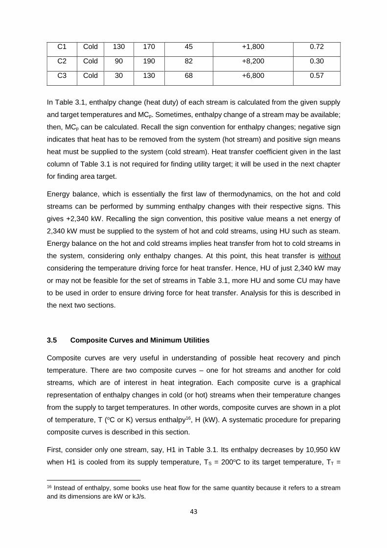
43
C1 Cold 130 170 45 +1,800 0.72
C2 Cold 90 190 82 +8,200 0.30
C3 Cold 30 130 68 +6,800 0.57
In Table 3.1, enthalpy change (heat duty) of each stream is calculated from the given supply
and target temperatures and MCp. Sometimes, enthalpy change of a stream may be available;
then, MCp can be calculated. Recall the sign convention for enthalpy changes; negative sign
indicates that heat has to be removed from the system (hot stream) and positive sign means
heat must be supplied to the system (cold stream). Heat transfer coefficient given in the last
column of Table 3.1 is not required for finding utility target; it will be used in the next chapter
for finding area target.
Energy balance, which is essentially the first law of thermodynamics, on the hot and cold
streams can be performed by summing enthalpy changes with their respective signs. This
gives +2,340 kW. Recalling the sign convention, this positive value means a net energy of
2,340 kW must be supplied to the system of hot and cold streams, using HU such as steam.
Energy balance on the hot and cold streams implies heat transfer from hot to cold streams in
the system, considering only enthalpy changes. At this point, this heat transfer is without
considering the temperature driving force for heat transfer. Hence, HU of just 2,340 kW may
or may not be feasible for the set of streams in Table 3.1, more HU and some CU may have
to be used in order to ensure driving force for heat transfer. Analysis for this is described in
the next two sections.
3.5 Composite Curves and Minimum Utilities
Composite curves are very useful in understanding of possible heat recovery and pinch
temperature. There are two composite curves – one for hot streams and another for cold
streams, which are of interest in heat integration. Each composite curve is a graphical
representation of enthalpy changes in cold (or hot) streams when their temperature changes
from the supply to target temperatures. In other words, composite curves are shown in a plot
of temperature, T (oC or K) versus enthalpy16, H (kW). A systematic procedure for preparing
composite curves is described in this section.
First, consider only one stream, say, H1 in Table 3.1. Its enthalpy decreases by 10,950 kW
when H1 is cooled from its supply temperature, TS = 200oC to its target temperature, TT =
16 Instead of enthalpy, some books use heat flow for the same quantity because it refers to a stream
and its dimensions are kW or kJ/s.

44
50oC. This change is given by ∆H = MCp (TT – TS), which can be re-arranged to (TS – TT) =
−∆H
MCp. Hence, cooling of H1 can be represented by the continuous straight line in Figure 3.5;
this is assuming MCp is constant. Left-most point of this T-H line has (x, y) coordinates of (0,
50) and right-most point has coordinates of (10,950, 200). Slope of the line for H1 stream is
1
MCp=
1
73 = 0.013699; this means slope of the line decreases as MCp increases and vice versa.
For plotting, it is more convenient to work with temperature changes and corresponding
enthalpy changes (i.e. with (x, y) coordinates of left- and right-most points).
Figure 3.5 shows two other straight lines: Dashed and dotted lines. What do they represent?
The dashed line on the right also represents cooling of H1 stream from its supply temperature,
TS = 200oC to its target temperature, TT = 50oC. Reasons for this are as follows: The dashed
line has two end points at the same temperatures as for the continuous line, and also its
enthalpy change is the same as that for the continuous line. Since enthalpy is with respect to
some reference point, enthalpy change should remain the same whereas starting and ending
enthalpy values are not fixed. Therefore, any straight line parallel to the continuous line and
within the same end temperatures represents cooling of H1 stream. In other words, the
continuous line can be shifted horizontally in the direction of x-axis. This is an important idea
in finding the utility target.
Figure 3.5: Stream H1 on temperature-enthalpy (T-H) plot
Consider the dotted line for which the two end temperatures are higher than those for H1
stream whereas the enthalpy change is the same as that for H1 stream. Does this dotted line

45
represent cooling of H1 stream? The answer is “No”, since the two end temperatures are
different (i.e. TS = 250oC and TT = 100oC in the case of the dotted line compared to TS = 200oC
and TT = 50oC in case of H1 stream). Therefore, T-H line representing any stream such as H1
can be shifted horizontally but not vertically.
For heat integration, there should be at least one hot stream and one cold stream. Figure 3.6
shows T-H lines of hot stream H1 and cold stream C2. The starting point of C2 stream at
enthalpy of 4,000 kW is arbitrary; however, enthalpy change of C2 stream is 8,200 kW, as
given in Table 3.1. Similar to the line for H1 stream in Figure 3.5, the line for C2 stream in
Figure 3.6 can be shifted horizontally (but not vertically).
In Figure 3.6, vertical distance between the red and blue lines at any x- (i.e. enthalpy) value is
the temperature driving force for heat transfer from H1 to C2 at that point. This driving force is
minimum (~15oC) at enthalpy of 4,000 kW (left vertical dashed line) and it is maximum (~25oC)
at enthalpy of 10,950 kW (right vertical dashed line). For a minimum driving force of 15oC,
thermal energy of H1 stream between the two vertical dashed lines can be transferred to C2
stream. In other words, energy of 10,950 – 4,000 = 6,950 kW can be recovered from H1 and
reused for C2. Another hot stream or HU is required for further heating of C2 beyond the right
vertical line; also, another cold stream or CU is needed for cooling H1 from ~105oC to 50oC.
Figure 3.6: Streams H1 (red line) and C2 (blue line) on temperature-enthalpy (T-H) plot
minimum temperature difference of ~15oC and heat recovery of 6,950 kW
What will be the heat recovery if the minimum temperature driving force is 10oC? For this, T-
H line for C2 stream is shifted horizontally to the left until the minimum driving force is 10oC,
Minimum Temperature Difference of
~ 15oC
Heat Recovery of 6,950 kW

46
as shown in Figure 3.7. This left-shifting widens the two vertical dashed lines and also
increases the heat recovery from H1 to C2 (to ~7,300 kW). What will be the heat recovery if
the minimum driving force is 20oC? For this, T-H line for C2 stream is shifted horizontally to
the right until the minimum driving force is 20oC; see Figure 3.8. This right-shifting reduces the
space between the two vertical dashed lines and also decreases the heat recovery from H1
to C2 (to ~6550 kW).
Owing to the limited accuracy of reading from the graph, reading values from a plot such as
that in Figures 3.6 to 3.8 will be approximate. However, accurate values can be calculated via
energy balance calculations using relevant interval and known temperatures and enthalpy
values. In any case, Figures 3.6 to 3.8 are effective in giving a visual picture of driving force
available for heat transfer, which affects heat exchanger size.
Usually, there will be more than one hot stream. How should the changes in all hot streams
be presented in the T-H plot? This can be done in the form of a hot composite curve for all hot
streams together. To learn this, consider two hot streams, H1 and H2 in Table 3.1, and perform
calculations for use in plotting the hot composite curve. These two streams together cover the
temperature range of 50oC to 200oC with both present in part of this range and only H1 present
in the remaining range of 140oC to 200oC.
Figure 3.7: Streams H1 (red line) and C2 (blue line) on temperature-enthalpy (T-H) plot -
minimum temperature difference of 10oC and heat recovery of ~7,300 kW
Minimum Temperature Difference of
10oC
Heat Recovery of ~7,300 kW

47
Figure 3.8: Streams H1 (red line) and C2 (blue line) on temperature-enthalpy (T-H) plot -
minimum temperature difference of 20oC and heat recovery of ~6,550 kW
As shown in Table 3.2, temperatures in the first column are the supply and target temperatures
of both H1 and H2, arranged in decreasing order. There are two temperature intervals: one is
from 200oC to 140oC, and another is from 140oC to 50oC. The second column shows the hot
stream(s) present in each temperature interval, and the third column has the sum of MCp of
streams present in that interval. The enthalpy change in each interval is then calculated in the
fourth column. This calculation is just for plotting the composite curve accounting for enthalpy
change in each temperature interval, and does not mean or require mixing of streams in any
interval. Enthalpy at each temperature in the last column of Table 3.2 is sum of absolute
enthalpy changes in intervals below that temperature, which means enthalpy at the lowest
temperature is zero. The data in the first and last column are used to plot the hot composite
curve, shown as red curve in Figure 3.9.
Table 3.2: Hot streams, their temperature intervals and enthalpies for plotting composite
curves
Temperature
(oC)
Streams
Present
MCp
(kW/K)
Enthalpy Change in the
Interval (kW)
Enthalpy at a
Temperature (kW)
200 14,460
H1 73 73(140-200) = -4380
140 10,080
H1, H2 73 + 39 (73+39)*(50-140) = -10,080
Minimum Temperature Difference of
20oC
Heat Recovery of ~6,550 kW

48
50 0
Figure 3.9: Hot composite curve (red curve) and cold composite curve (blue curve) for the
stream data in Table 3.1
Note that zero enthalpy at the lowest temperature leads to the starting of the hot composite
curve at x = 0.0 kW. This is a convenient option. Also, observe the arrangement of rows in
Table 3.2; this is such that temperature and enthalpy in columns 1 and 5 are in one row
followed by values in columns 2 to 4 in the next row. This facilitates not only calculations but
also their interpretation and use. This arrangement will be followed in several other tables in
this chapter.
The 2 segments of the hot composite curve in Figure 3.9 correspond to the 2 temperature
intervals in Table 3.2. In the first segment/interval of 200oC to 140oC, there is only one stream
(H1) whereas there are 2 streams (H1, H2) in the second segment/interval from 140oC to
50oC. In this way, using the composite curve and data used for plotting it, streams present in
each segment can be found. Notice the change in the slope of the line from one segment to
another.
Next, Table 3.3 shows the required data and calculations for plotting the cold composite curve
for the three cold streams in Table 3.1. With three cold streams, there are more intervals and
calculations in Table 3.3. Temperatures in the first column of this table are in increasing
Segment with only H1 stream
Segment with both H1 and H2
streams Segment with C2 and C3 streams
Segment with C1 and C2 streams
Segment with only C1 stream
Segment with only C3 stream

49
sequence, similar to increasing temperature of cold streams. Data and calculations in columns
2 to 4 are similar to those in Table 3.2 for hot streams.
Table 3.3: Cold streams, their temperature intervals and enthalpies for plotting composite
curves
Temperature
(oC)
Streams
Present
MCp
(kW/K)
Enthalpy Change in the
Interval (kW)
Enthalpy at a
Temperature (kW)
30 3,000
C3 68 68(90-30) = + 4,080
90 7,080
C2, C3 82+68 (82+68)(130-90) = +6,000
130 13,080
C1, C2 45+82 (45+82)(170-130) = +5,080
170 18,160
C2 82 82(190-170) = +1,640
190 19,800
Enthalpy calculations in the last column of Table 3.3 are starting with an arbitrary value (here,
3,000 kW) so that the cold composite curve begins on the right of the y-axis. Also, enthalpy at
a temperature is the sum of this arbitrary value and all enthalpy changes above that
temperature. The plot of temperature in the first column of Table 3.3 versus enthalpy in the
last column gives the cold composite curve, shown as blue curve in Figure 3.9. The cold
composite curve consists of 4 segments corresponding to 4 intervals in Table 3.3, and the
slope (= 1/MCp) in each segment is different.
What can be deduced from the two composite curves in Figure 3.9? Firstly, heat recovery is
in the zone between the two vertical dashed lines at 3,000 kW (starting point of cold composite
curve in Table 3.3) and 14,460 kW (ending point of hot composite curve in Table 3.2), and it
is equal to 14,460 – 3,000 = 11,460 kW. Secondly, for this heat recovery, minimum
temperature driving force, (∆T)min (difference between hot and cold streams) is ~23oC,
identified by the small vertical dashed line at enthalpy 7,080 kW (based on Table 3.3). This
particular point is known as ‘pinch’, whose significance will be discussed in the later part of
this chapter. It usually occurs at the point where the slope of a composite curve (either hot or
cold) changes.

50
Finally, towards the right end of the cold composite curve (after the vertical dashed line), HU
is required for heating and it is 5,340 kW. This value can be read approximately from Figure
3.9 or can be obtained as the difference between the largest enthalpies in Tables 3.2 and 3.3
(i.e. 19,800 – 14,460 = 5,340). CU of 3,000 kW is required for cooling hot streams to the left
of the left-most vertical dashed line.
The HU of 5,340 kW and CU of 3,000 kW are the minimum utilities required for (∆T)min of
~23oC. Is it possible to find the minimum utilities for a given (∆T)min, say, 10oC? Yes, minimum
utilities for any given (∆T)min can be found by shifting the cold composite curve in Figure 3.9.
For a lower (∆T)min, this shifting is towards left side. How far should this shifting be? For this,
starting enthalpy in Table 3.3 can be calculated based on the following: Pinch occurs at cold
stream temperature of 90oC in Figure 3.8, hot stream temperature at pinch should be 100oC
for (∆T)min = 10oC and so enthalpy of hot composite curve can be calculated, based on data in
Table 3.2, as 10,080 + (73+39)*(100-140) = 5,600. Hence, the cold composite curve should
be shifted to left by 7,080 – 5,600 = 1,480. This can be done by reducing the arbitrarily chosen
enthalpy of 3,000 kW in Table 3.3 by 1,480 to 1,520 kW, and re-plotting cold composite curve,
as shown in Figure 3.10. Obviously, these values will be different for a different example but
similar calculations can be performed for shifting the cold composite curve.
Figure 3.10: Hot composite curve (red curve) and cold composite curve (blue curve) for the
stream data in Table 3.1 and (∆T)min = 10oC
Min. HU
Min. CU
Energy Recovery
Pinch

51
In Figure 3.10 for (∆T)min = 10oC, energy recovery is 12,940 kW, which is equal to the difference
in enthalpy at the end of hot composite curve (14,460) and starting point of cold composite
curve (1,520). Pinch is at hot stream temperature of 100oC and cold stream temperature of
90oC. The minimum HU is 3,860 kW (reduced from the earlier value of 5,340 by 1,480 because
of shifting the cold composite curve to left), and minimum CU is 1,520 kW. In short, with a
lower (∆T)min, energy recovery increases and both hot and cold utilities decrease, all by the
same amount (here, by 1,480 kW).
In other words, if more CU is used for a set of process streams, then more HU is required.
This is the result of energy balance that must be satisfied by enthalpy changes in hot and cold
streams together with hot and cold utilities supplied. One way to write this energy balance is
as follows:
Energy given by hot streams + HU = Energy taken by cold streams + CU.
The difference between hot utilities and cold utilities for (∆T)min = 10oC (Figure 3.9) is 3860 –
1,520 = 2,340 kW. This value is exactly same as the difference between hot utilities and cold
utilities for (∆T)min = 23oC (Figure 3.8) is 5,340 – 3,000 = 2,340 kW. Both of these are again a
result of energy balance.
In summary, the procedure for finding minimum utilities using the composite curves is as
follows.
1. Collect stream data as in Table 3.1.
2. Prepare a table for hot streams, their temperatures, intervals and enthalpy changes (such
as Table 3.2).
3. Prepare another table for cold streams, their temperatures, intervals and enthalpy changes
(such as Table 3.3). Choose a reasonable initial enthalpy (in the first row of Table 3.3).
4. Use temperatures and enthalpies from the above two tables to plot hot and cold composite
curves. Choose range for x-axis to be much more than the maximum enthalpy in Table 3.2
since the cold composite curve is likely to extend beyond the hot composite curve.
5. Revise the initial enthalpy for the cold composite curve such that minimum temperature
difference between hot and cold streams is equal to the given (∆T)min.
6. Find the following from the composite curves: Energy recovery, pinch, minimum HU and
minimum CU.
Depending on the stream data, minimum HU can be more (as in Figure 3.10) or less (as in
Figure 3.6) than minimum CU. In a number of applications, only one utility (either hot or cold)
is required. Such problems are referred to as threshold problems, and they are discussed in
a later chapter.

52
3.6 Problem Table Procedure for Finding Minimum Utilities
Problem table procedure, also known as temperature interval analysis, is numerical alternative
to graphical method of composite curves, for finding the minimum cold and hot utilities along
with pinch and energy recovery. It does not involve iterations (i.e. shifting composite curves)
and gives accurate results (assuming no mistake in the calculations). Problem table procedure
is described in this section for the stream data in Table 3.1 used earlier for describing
composite curves.
Recall that pinch in Figure 3.10 is at hot stream temperature of 100oC and cold stream
temperature of 90oC. Thus, at any point (e.g. enthalpy in Figure 3.9), pinch analysis uses two
temperatures, namely, hot stream temperature (HST) and cold stream temperature (CST). In
addition, shifted temperature (ST) is defined as the mean of HST and CST. A few examples
of HST, ST and CST are as follows.
If HST = 100oC and CST = 90oC (which implies (∆T)min = 10oC), then ST = 95oC.
If HST = 140oC and CST = 130oC (which implies (∆T)min = 10oC), then ST = 135oC.
If HST = 80oC and CST = 60oC (which implies (∆T)min = 20oC), then ST = 70oC.
In general, ST = HST – (∆T)min
2 and also ST = CST+
(∆T)min
2; alternatively, HST = ST+
(∆T)min
2
and CST = ST – (∆T)min
2.
The stream data in Table 3.1 is repeated in Table 3.4 along with ST for each supply/target
temperature, for (∆T)min = 10oC. Figure 3.11 can now be prepared using ST values in Table
3.4 in decreasing order, to show the streams and their temperatures. Note that this figure is
schematic and does not use a scale for temperatures. In Figure 3.11, HST, ST and CST are
respectively in the left, centre and right long rectangles; the interval number is given in circle
between the two STs. Further, HST and CST at any level (i.e. dashed line) differs by (∆T)min =
10oC. This means heat from hot streams present in any interval can be transferred to cold
streams present in that interval, while ensuring (∆T)min for heat transfer. However, total heat
available in all hot streams in any interval may be more than, equal to or less than the total
heat required by all cold streams in that interval.
Table 3.4: Stream data for heat integration; shifted temperature (ST) is given in brackets
after each supply/target temperature
Stream Type TS (°C) TT (°C) MCp (kW/°C) Enthalpy Change (kW)
H1 Hot 200 (195) 50 (45) 73 -10,950

53
H2 Hot 140 (135) 50 (45) 39 -3,510
C1 Cold 130 (135) 170 (175) 45 1,800
C2 Cold 90 (95) 190 (195) 82 8,200
C3 Cold 30 (35) 130 (135) 68 6,800
Using Figure 3.11, problem table procedure is performed in Table 3.5. The first two columns
of this table are ST and interval number, the third column is temperature change in the interval
(= difference between two consecutive STs) and the fourth column contains streams present
in an interval. The difference between the sum of MCp of hot streams and the sum of MCp of
cold streams present in each interval, is calculated in the fifth column. Then, the energy in an
interval, ∆H is the product of third column (Si – Si+1) and fifth column (MCp,h - MCp,c). This is
the net energy in an interval after heat transfer among hot and cold streams present in that
interval, to satisfy the requirement of either hot or cold streams (and not both set of streams).
Figure 3.11: Schematic of, from left to right, HST, hot streams, ST, intervals, cold streams
and CST

54
Table 3.5: Problem table procedure for stream data in Table 3.4 and Figure 3.11
ST, Si
(oC)
Interval
No. i
Si –
Si+1
Streams
Present
MCp,h -
MCp,c
(kW/oC)
H
(kW)
Surplus
or
Deficit
Heat
Cascade
(kW)
Feasible Heat
Cascade
(kW)
195 0 3,860
1 20 H1, C2 73-82
= - 9
-180 D
175 -180 3,680
2 40 H1, C1,
C2
73-45-82
= - 54
-2,160 D
135 -2,340 1,520
3 40 H1, H2,
C2, C3
73+39-82-
68 = - 38
-1,520 D
95 -3,860 0
4 50 H1, H2,
C3
73+39-68
= + 44
+2,200 S
45 -1,660 2,200
5 10 C3 - 68 -680 D
35 -2,340 1,520
Net energy is positive (surplus) if the change in enthalpy of hot streams present in an interval
is more than that of cold streams present in the same interval. It is negative (deficit) if the
enthalpy change of hot streams is less than that of cold streams, in the interval. For example,
consider interval no. 2; in this interval, absolute enthalpy change of H1 present is 7340 =
2,920 kW, whereas that of C1 and C2 present is (45+82) 40 = 5,080 kW. After transferring
all heat in H1 to C1 and C2 present in the interval, C1 and C2 require energy of 5,080 – 2,920
= 2,160 kW. This gives the net energy of -2,160 kW. Note that these calculations are for
analysis only, and there is no mixing of cold (or hot) streams in any interval.
The next question in the problem table procedure is how to satisfy the deficit and surplus in
the last column of Table 3.5. One possibility is to use CU for removing the surplus heat and to
use HU for providing the deficit heat. This is not energy efficient, and there is a better strategy.
For example, the surplus in interval 4 can be used in a lower interval (i.e. at a lower
temperature). This leads to the idea of heat cascade starting with zero heat flow at the top, as

55
shown in the second last column of Table 3.5. The value in the last row (-2,340) is essentially
the algebraic sum of all ∆H in the sixth column.17
Heat cascade consists of a series of heat flows (or net heat flows), as shown in the second
last column of Table 3.5. Significance of heat cascade is as follows. Starting with zero heat
flow at the top, heat flow entering an interval from the top and H in that interval are added to
find the heat flow leaving that interval into the next interval. For example, heat flow entering
interval 2 is -180 kW and H in interval 2 is -2,160; sum of these two values is -2,340 kW,
which is the heat flow leaving interval 2 and going to interval 3.
Negative heat cascade means heat is transferred from a lower interval (temperature) to a
higher interval (temperature), which is not possible (unless additional energy is spent (as in
air conditioning). This is similar to pumping water from ground level to a higher level. On the
other hand, positive heat cascade means heat is transferred from a higher interval
(temperature), which is possible similar to water falling from a higher level to a lower level.18
Since negative heat flow is not feasible, heat cascade in the second last column of Table 3.5
is not feasible. To obtain feasible heat cascade, heat has to be supplied at the top such that
heat flow is either zero or positive throughout. In Table 3.5, this is achieved by supplying 3,860
kW of energy in the form of HU, at the top; this quantity is the smallest (most negative) heat
flow in the second last column of the table. Feasible heat cascade is in the last column of
Table 3.5; each value in this column can be obtained by adding 3,860 to the corresponding
heat flow in the (infeasible) heat cascade in the second last column.
Heat cascade diagram (i.e. diagram of net heat flow from a higher temperature to a lower
temperature) for the example data in Table 3.5 is illustrated in Figure 3.12. It presents shifted
T, net energy in each of interval, and infeasible and feasible heat cascades.
17 This value means the cold and hot streams in the problem requires external energy in order to achieve
their respective target temperatures. This is the same as that found by energy balance in Section 3.4.
This observation can be used to check calculations for problem table procedure, by comparing sum of
all ∆H with that obtained from energy balance on all cold and hot streams.
18 In Table 3.5, there is no positive heat cascade in this problem. Some positive heat cascades can be
seen in Exercise Question 4 at the end of this chapter.

56
Figure 3.12: Heat cascade diagram for the example data in Table 3.5
The following can be deduced from the feasible heat cascade in the last column of Table 3.5.
Minimum HU required is 3,860 kW, minimum CU is 1,520 kW (since heat cascade at the
bottom has to be removed using a CU), and pinch is at ST = 95oC (i.e. HST = 100oC and CST
= 90oC since (∆T)min = 10oC), where heat flow is zero. The energy recovered can be calculated
by subtracting minimum CU from the total energy given by hot streams. For the example under
study, energy given by hot streams is 10,950 + 3,510 = 14,460 kW from Table 3.1, and hence
energy recovery is 14,460 – 1520 = 12,940 kW. These results are exactly the same as those
found from the composite curves.
If more than the minimum HU (i.e. > 3,860 kW) is used, then more CU is required and there
is no pinch. This will increase the utility cost for the heat exchanger network (HEN) although
its capital cost may be lower.
Heat cascade will obviously depend on the stream data in the problem. In some problems,
there may be no negative heat flow in the second last column of Table 3.5, and pinch may be
at one end of the heat cascade. In some other problems, there may be more than one pinch.
Some of these situations can be seen in Exercise Question.4 at the end of this chapter.
In summary, the problem table procedure (also known as temperature interval analysis)
consists of column-by-column calculations starting from the left column in a table such as
Table 3.5. Figure 3.11 is useful for learning problem table procedure. After sufficient

57
experience on its application, problem table procedure can be performed without preparing
stream data as in Figure 3.11. However, observe and carefully follow the arrangement of rows
in Table 3.5; temperature (in the first column) and heat cascades (in the last two columns) are
in one row followed by the next row for values in the remaining columns. This is similar to the
row arrangement in Table 3.2.
3.7 Pinch and its Significance
Both composite curves and problem table procedure give pinch temperature (Pinch) besides
minimum utility targets. Pinch is significant with a number of implications for HEN design.
These are described in this section.
Pinch is where the driving force for heat transfer is equal to (∆T)min, and the heat flow across
the pinch is zero. When available driving force for heat transfer is small, HEN design is more
difficult; this is similar to managing limited budgets in life or at work. Thus, the region near the
pinch is more constrained. Hence, HEN should be developed starting with designs near (and
not far away from) the pinch. This is different from one conventional practice of HEN design
that starts from the high-temperature end of streams and without considering targets and
pinch.
Since heat flow across the pinch is zero, hot and cold streams above pinch temperature and
minimum HU are in energy balance. In other words, the following equation is satisfied for the
red dashed envelope in Figure 3.13: (sum of absolute enthalpy changes of hot streams
between their respective supply temperatures and pinch temperature) + minimum HU = (sum
of absolute enthalpy changes of cold streams between pinch temperature and their respective
target temperatures). Similarly, hot and cold streams below pinch temperature and minimum
CU are in energy balance (in blue dashed envelope in Figure 3.13).

58
Figure 3.13: Composite curves showing above pinch region (red dashed envelope) and
below pinch region (blue dashed envelope) for the stream data in Table 3.1 and (∆T)min =
10oC
The energy balances in the previous paragraph arising from no heat flow across the pinch (i.e.
from red envelope to blue envelope), imply HEN design above pinch and HEN design below
pinch can be carried out independently by the same or different persons. In other words, the
larger design problem of complete HEN is divided into two sub-problems of relatively smaller
HEN design. Since a larger design problem is more complex and difficult than smaller HEN
design, this division into two sub problems is useful and convenient.
Above pinch, only minimum HU and no CU should be used. If q kW of more HU is used, then
CU will increase by q kW for later removal of more HU used. Similarly, if some CU is used
above pinch, then required HU will increase by the same amount. Below pinch, only minimum
CU and no HU should be used.
In summary, at the pinch, temperature driving force for heat transfer is equal to (∆T)min and
heat flow is zero. It increases design flexibility by dividing the larger HEN problem into two
sub-problems: design above and design below pinch. Arising from the pinch and its
implications, the following are the golden rules for the HEN design by pinch analysis, covered
in later chapters.
1. No heat flow across the pinch.
2. Only HU (and no CU) above the pinch
Min.
CU
Min.
HU
Pinch

59
3. Only CU (and no HU) below the pinch.
The above golden rules are shown pictorially on the composite curves in Figure 3.14.
Figure 3.14: Composite curves with the three golden rules and minimum utilities for
maximum energy recovery
Violation of any of the above golden rules increases cold and/or hot utilities above the
minimum targets found for the given (∆T)min using composite curves or problem table
procedure. Examples of golden rule violations and corresponding penalties are (Figure 3.15):
1. a heat flow of 200 kW across pinch (say, from a hot stream above pinch to a cold
stream below pinch) increases both HU and CU by 200 kW;
2. use of 100 kW of CU above pinch increases HU by 100 kW; and
3. use of 50 kW of HU below pinch increases CU by 50 kW.
In a HEN designed without following pinch analysis, one or more golden rules may be violated.
In such a case, total penalty in utilities above the minimum targets is equal to sum of penalty
of each of violations of golden rules (Figure 3.15).
No HU
below Pinch
No CU
above Pinch
No Heat Flow
Across Pinch
Min. HU
Min. CU

60
Figure 3.15: Violation of golden rules and corresponding penalty in increasing utilities
Plus-Minus Principle: Recall the following findings from the previous section: (a) zero heat
flow across the pinch, (b) cold and hot streams present along with HU above pinch are in
energy balance, and (c) cold and hot streams along with CU below pinch are in energy
balance. These provide guidance on suitable changes in the rest of the process for reducing
cold and hot utilities.
Any process change that increases total duty of hot streams above pinch can decrease
HU.
Any process change that decreases total duty of cold streams above pinch can
decrease HU.
Any process change that increases total duty of cold streams below pinch can
decrease CU.
Any process change that decreases total duty of hot streams below pinch can
decrease CU.
The above are collectively known as plus-minus principle. They are useful in finding
appropriate changes in design and operating conditions of the rest of the process. One
example is distillation column pressure that affects temperatures of condenser and reboiler
(i.e. hot and cold streams). Increase in column pressure can shift the hot stream (condenser
HU of 50
kW below
Pinch
CU of 100 kW
above Pinch
Min. HU
+ 200 + 100
Heat Flow of 200
kW Across Pinch
Min. CU
+ 200 + 50

61
duty) from below to above pinch point whereas decrease in column pressure can shift the cold
stream (reboiler duty) from above to below pinch. For more details and applications of plus-
minus principle, see Chapters 20 to 22 in Smith (2005).
3.8 Summary
This chapter covers the first two steps in pinch analysis for heat integration. The first step is
extracting stream data from the operating plant or design of a new plant. Guidelines for
choosing cold and hot streams as well as for finding stream data for heat integration are
described with examples. For more details on these and examples, see Chapter 19 in Smith
(2005). The second step is finding the minimum cold and hot utilities along with pinch.
Systematic procedure for this consists of energy balance on all streams followed by application
of problem table procedure (for accurate values) or composite curves (for visual picture of
driving forces) to find CU, HU and pinch. Second step is illustrated using an example having
2 hot streams and 3 cold streams.
Pinch is an important concept in pinch analysis; driving force for heat transfer at pinch is equal
to (∆T)min, and the heat flow across the pinch is zero. It can be found from either problem
table procedure or composite curves. Significance of pinch is described and the consequent
golden rules for the HEN design are listed. For application of problem table procedure and
composite curves to other examples, see Chapter 2 in Kemp (2007) and Chapter 16 in Smith
(2005). Note that each of these books follows different conventions for heat transfer and/or
equations for calculations.
3.9 References
Kemp I.C., Pinch Analysis and Process Integration: A User Guide on Process Integration for
Efficient Use of Energy, 2nd Edition, Butterworth-Heinemann (2007).
Smith R., Chemical Process Design and Integration, John Wiley (2005).

62
3.10 Exercises
1. Consider condensing/cooling 10 kg/s of a vapour mixture of 50 wt% ethanol and 50 wt%
from 103oC to 40oC. It is stated that this processing step can be taken as two streams.
Based on the values given in Section 3.2, find the data of each of these two streams.
Are these hot or cold streams?
2. For the stream data in Table 3.1 and (∆T)min = 20oC, find the minimum utilities, energy
recovered and pinch using the composite curves. Confirm the results found by applying
the problem table procedure to the same data and (∆T)min = 20oC. (Answers: minimum
hot utility = 4,980 kW, minimum cold utility = 2,640 kW, energy recovered = 11,820 kW
and pinch at 110/90oC)
3. Study the following process developed by a young engineer. Is the flow sheet achieving
maximum energy recovery (i.e. using minimum utilities)? Assume the following: (a)
steam at 250oC is used in both the heaters; (b) cooling water is available at 20oC and
should be returned at 40oC; (c) heat exchangers, heaters and cooler are of counter-
current type; and (d) steady state operation. Suggested steps are: (i) find the hot utility
and cold utility used in the developed process; (ii) find the hot streams and cold streams
in the process, and their MCp, supply and target temperatures; (iii) find the approach
temperatures of each heat exchanger, heater and cooler; (iv) select minimum
temperature driving force, (∆T)min equal to the minimum approach temperature; (v) find
the hot and cold utility targets for the assumed (∆T)min; and (iv) compare the targets
with the hot and cold utilities used in the developed process. This procedure can be used
for analysing energy recovery and effectiveness of a new or existing heat exchanger
network. See also Exercise Question 5.
Feed
MCp = 3 kW/oC
1
2
Reactor
Separator
Effluent,
MCp = 6 kW/oC
Product
Recycle
MCp = 2 kW/oC
25oC 145oC 200oC 180oC
100oC 200oC
40oC
120oC
100oC 40oC

63
4. Results from the application of problem table procedure to process streams in 4 different
plants are summarised in Tables E1 to E4. For each of them, study the heat cascade in
column 3, state (∆T)min used, provide feasible cascade in column 4, and then find the
pinch and minimum utilities. Note that stream data and ∆H in each interval are not given
as they are not required for this exercise.
Table E1: Results from problem table procedure of process streams: Set A
HST
(oC)
CST
(oC)
Heat Cascade: Feasible
or Infeasible? (kW)
Feasible
Cascade (kW)
340 330 0
300 290 21.6
270 260 -16.2
200 190 -90.4
160 150 -139.2
130 120 -106.8
90 80 -22.4
80 70 -6.7
40 30 -43.9
Table E2: Results from temperature interval analysis of process streams: Set B
HST
(oC)
CST
(oC)
Heat Cascade: Feasible
or Infeasible? (kW)
Feasible
Cascade (kW)
590 570 0
533 513 135.4
471 451 364.6
450 430 475.3
420 400 585.5
400 380 544.4
320 300 189.9
300 280 183.9
220 200 -50.3
200 180 -76.8

64
170 150 -164.0
150 130 -169.6
120 100 -217.6
Table E3: Results from temperature interval analysis of process streams: Set C
HST
(oC)
CST
(oC)
Heat Cascade: Feasible
or Infeasible? (MW)
Feasible
Cascade (MW)
150 140 0
140 130 6
130 120 8
100 90 44
50 40 54
30 20 66
Table E4: Results from temperature interval analysis of process streams: Set D
HST
(oC)
CST
(oC)
Heat Cascade: Feasible
or Infeasible? (kW)
Feasible
Cascade (kW)
500 480 0
470 450 120
440 420 210
420 400 255
201 181 529
200 180 0
100 80 125
80 60 70
70 50 52.5
60 40 45
5. An existing heat exchanger network in a specialty chemical plant is shown in the figure
below. Value near each heat exchanger in this figure refers to heat load of the
exchanger/heater/cooler.

65
210 kW 50 kW
100 kW 170 kW
116 kW
S2 HU S1
S4
CU
S3
Stream data are given in the table below. Based on current economic environment,
minimum driving force of 200C is considered to be the optimum. Compared to the hot
utility target for this minimum driving force, how much more hot utility is being used in
the existing heat exchanger network?
Stream
No.
Supply
Temp. (0C)
Target
Temp. (0C)
MCp
(kW/0C)
S1 320 200 1.8
S2 480 290 2.0
S3 240 500 1.0
S4 140 320 1.5
6. Carefully study each of the following statements and state whether each of them is
correct/true or wrong/false.
(A) MCp of a stream is always based on heat capacity or specific heat of the stream.
(B) A stream may have to be taken as two streams if Cp is varying significantly or if
phase change is involved.
(C) Energy balance on all cold and hot streams in a particular application gives net
cold or hot utility required. This may or may not be achievable in practice.
(D) Hot composite curve can be shifted horizontally and vertically on the T-H plot.
(E) Cold composite curve can be shifted horizontally on the T-H plot.
(F) Shifted temperature is equal to hot stream temperature.

66
(G) Shifted temperature is more than cold stream temperature.
(H) Heat cascade involving one or more negative (heat flow) values is infeasible.
(I) A feasible heat cascade has always only one zero (heat flow) value.
(J) For maximum energy recovery, there should be no heat flow across the pinch point.
(K) There is only one pinch point in all heat integration problems.

67
Chapter 4
Pinch Analysis: Number of Units, Heat Transfer Area and
Supertargeting
By
Gade Pandu Rangaiah
4.1 Overview
The previous chapter described extraction of the required stream data from the process
flowsheet and/or operating plant, and then two methods for finding the minimum utilities and
pinch for the given minimum temperature driving force, (∆T)min. Minimum utilities is the first
target found before heat exchanger network (HEN) design. In this chapter, methods for finding
the minimum number of units and heat transfer area required, both before the HEN design,
are described in Sections 4.2 and 4.3, respectively. Here, the term ‘units’ refers to all heat
exchangers including heaters and coolers in the HEN, and not to dimensions such as kW and
m2. Also, heat transfer area refers to the total area in all units in the HEN to be designed later.
After knowing minimum utilities, number of units and total heat transfer area, operating cost
(OC) and capital cost (CC) can be estimated without HEN design. Usually, OC and CC are
conflicting (i.e OC is lower when CC is higher and vice versa). Estimates of these costs form
the basis for finding the optimum (∆T)min to minimise total annual cost (TAC), which accounts
for both OC and CC. This procedure is known as supertargeting in pinch analysis, and it is
described in Section 4.4. Summary of this chapter on finding important quantities before the
HEN design is given in Section 4.5.
The following are the learning outcomes of this chapter on number of units, heat transfer area
and supertargeting in pinch analysis.
1. Find the minimum number of units in the HEN with or without pinch point
2. Describe the procedure for the finding total heat transfer area required
3. Calculate the total heat transfer area required before the HEN design
4. Estimate OC and CC before the HEN design
5. Describe supertargeting to find the optimum (∆T)min

68
4.2 Target on Number of Units
Number of units refers to the total number of heat exchangers including heaters and coolers.
It does not refer to dimensions such as oC, kJ/s and $/year. Target on number of units means
the minimum number of units (denoted by Umin) in the HEN yet to be designed. The equation
for finding this target is simple but care should be exercised in using it. Let’s first consider
stream data in Table 3.1, reproduced as Table 4.1 for ready reference. Temperatures and
heat transfer coefficient (h) of steam (hot utility, HU) and cooling water (cold utility, CU) are
also added in Table 4.1. Note that h for each stream is the combined coefficient accounting
for both film and fouling coefficients, and h values for steam condensation and cooling water
are based on lower values in the ranges given in Table 2.1.
Table 4.1: Stream data for heat integration in a large petrochemical plant
Stream Type TS (°C) TT (°C) MCp (kW/K) Enthalpy Change (kW) h (kW/m2.K)
H1 Hot 200 50 73 -10,950 0.18
H2 Hot 140 50 39 -3,510 0.65
Steam HU 215 215 - - 2.5
Cooling
Water CU 30 45 - - 1.2
C1 Cold 130 170 45 +1,800 0.72
C2 Cold 90 190 82 +8,200 0.30
C3 Cold 30 130 68 +6,800 0.57
In the previous chapter, for the stream data in Table 4.1 and (∆T)min = 10oC, minimum HU and
minimum CU are found to be 3,860 kW and 1,520 kW, respectively. Instead of these minimum
utilities, assume 4,860 kW of HU and 2,520 kW of CU (i.e. 1,000 kW more than the minimum
of HU and CU) are to be used. (Minimum utilities case is discussed later.) These HU, CU and
enthalpy changes (without sign for simplicity) of 2 hot streams and 3 cold streams in Table 4.1
can be represented as in Figure 4.1. In case of HU and CU, enthalpy change is equal to the
utility quantity (in terms of energy units) required.
Note that, in Figure 4.1, sum of enthalpy changes of hot streams and HU (= 10,950 + 3,510 +
4,860 = 19,320 kW) is exactly equal to sum of enthalpy changes of cold streams and CU (=
1,800 + 8,200 + 6,800 and 2,520 = 19,320 kW). This is because of energy balance among all
streams and utilities involved, and the assumption of no heat loss from any stream or utility or
unit, which is reasonable for preliminary analysis.

69
Figure 4.1: Hot streams and HU (in the top row) and cold streams and CU (in the lower row)
with absolute enthalpy change in kW (in brackets)
Units (heat exchangers) are required for transferring energy from hot streams and HU to cold
streams and CU, which can be as shown in Figure 4.2. In this figure, each arc (curve
connecting from a hot stream/HU to a cold stream/CU) requires one unit, and its duty (heat
transferred) is shown in the adjacent rectangle. In total, the required number of units is 6,
which is the minimum. Other configurations of minimum number of units (besides that in Figure
4.2 are possible. One alternate configuration is presented in Figure 4.3, wherein HU and CU
are placed on the left side, purely for easy drawing of arcs. In this too, minimum number of
units is 6.
Figure 4.2: Heat transfer (value in kW shown in square boxes) from hot streams and HU to
cold streams and CU
In both Figures 4.2 and 4.3, minimum number of units is obtained by maximising the heat
transferred in each unit (as much as possible considering enthalpy change of the two streams
involved). This strategy is used in the HEN design later in the next chapter. Is a configuration

70
with 5 or fewer units possible for the streams and utilities in Figure 4.1? The answer is no.
However, more units can be used by changing/reducing heat transferred in some units and
adding more arcs.
Figure 4.3: Alternate heat transfer configuration to that shown in Figure 4.2
Minimum number of units is given by the simple equation:
Umin = nh + nc + nu - 1 (4.1)
Here, nh, nc and nu are the number of hot, cold and utility streams, respectively; nu includes
both cold and hot utilities. Proof of this equation is based on graph theory, and it is beyond the
scope of this reference manual. However, Equation 4.1 can be verified for streams In Figure
4.1, wherein nh = 2, nc = 3 and nu = 2, and so Umin = 2 + 3 + 2 – 1 = 6, as can be seen in
Figures 4.2 and 4.3.
Now, let’s decrease enthalpy change of H1 by 950 kW to 10,000 kW, and also increase
enthalpy change of H2 by 950 kW to 4,460 kW; this decrease and increase are in order to
satisfy the energy balance of all streams and utilities involved. According to Equation 4.1, Umin
for this modified scenario is still 6. On the other hand, study the configuration in Figure 4.4
with only 5 units. Is it correct? Indeed, it is possible. Modified stream data in Figure 4.4 is a
very special situation. Here, enthalpy change of H1 is exactly equal to sum of enthalpy
changes of C1 and C2; and sum of enthalpy changes of H2 and HU (= 4,460 + 4,860 = 9,320)
is equal to sum of enthalpy changes of C3 and CU (= 6,800 + 2,520 = 9,320). In this special
situation, streams involved (namely, 2 hot streams, HU, 3 cold streams and CU) can be
grouped into 2 subsets: H1, C1 and C2 form one subset, and H2, HU, C3 and CU form second
subset.
For the (original) streams in Figure 4.1, there is only one subset. Equation 4.1 is valid for such
cases where all process streams and utilities form only one subset. For more than one subset,
the constant (1) on the right side of Equation 4.1 should be replaced by number of subsets
(ns) (= 2 for streams/utilities in Figure 4.4). In other words,

71
Umin = nh + nc + nu - ns (4.2)
The above equation can be written in words as
Umin = number of streams including utilities – number of subsets (4.3)
In real problems, enthalpy changes will not be round numbers, and so more than one subset
is very unlikely.
Figure 4.4: Heat transfer configuration for the modified enthalpy changes of H1 and H2,
which result in two subsets
Stream and utility data in Figure 4.1 do not correspond to minimum utilities. As found in
Chapter 3, for the stream data in Table 4.1 and (∆T)min = 10oC, minimum HU and minimum
CU are 3,860 kW and 1,520 kW, respectively. Moreover, pinch is at hot stream temperature
of 100oC and cold stream temperature of 90oC, and it divides the HEN problem into two sub-
problems, one above the pinch and another below the pinch. Streams and their temperatures
are shown in Figure 4.5 (reproduced from Figure 3.10 for ready reference).
Figure 4.5: Schematic of hot and cold streams with their temperatures; pinch is at 100/90oC
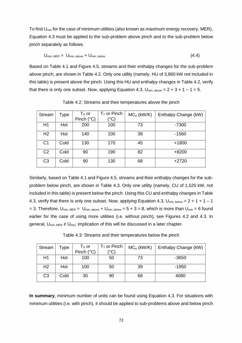
72
To find Umin for the case of minimum utilities (also known as maximum energy recovery, MER),
Equation 4.3 must be applied to the sub-problem above pinch and to the sub-problem below
pinch separately as follows.
Umin, MER = Umin, above + Umin, below (4.4)
Based on Table 4.1 and Figure 4.5, streams and their enthalpy changes for the sub-problem
above pinch, are shown in Table 4.2. Only one utility (namely, HU of 3,860 kW not included in
this table) is present above the pinch. Using this HU and enthalpy changes in Table 4.2, verify
that there is only one subset. Now, applying Equation 4.3, Umin, above = 2 + 3 + 1 – 1 = 5.
Table 4.2: Streams and their temperatures above the pinch
Stream Type TS or
Pinch (°C)
TT or Pinch
(°C) MCp (kW/K) Enthalpy Change (kW)
H1 Hot 200 100 73 -7300
H2 Hot 140 100 39 -1560
C1 Cold 130 170 45 +1800
C2 Cold 90 190 82 +8200
C3 Cold 90 130 68 +2720
Similarly, based on Table 4.1 and Figure 4.5, streams and their enthalpy changes for the sub-
problem below pinch, are shown in Table 4.3. Only one utility (namely, CU of 1,520 kW, not
included in this table) is present below the pinch. Using this CU and enthalpy changes in Table
4.3, verify that there is only one subset. Now, applying Equation 4.3, Umin, below = 2 + 1 + 1 – 1
= 3. Therefore, Umin, MER = Umin, above + Umin, below = 5 + 3 = 8, which is more than Umin = 6 found
earlier for the case of using more utilities (i.e. without pinch); see Figures 4.2 and 4.3. In
general, Umin, MER ≥ Umin; implication of this will be discussed in a later chapter.
Table 4.3: Streams and their temperatures below the pinch
Stream Type TS or
Pinch (°C)
TT or Pinch
(°C) MCp (kW/K) Enthalpy Change (kW)
H1 Hot 100 50 73 -3650
H2 Hot 100 50 39 -1950
C3 Cold 30 90 68 4080
In summary, minimum number of units can be found using Equation 4.3. For situations with
minimum utilities (i.e. with pinch), it should be applied to sub-problems above and below pinch

73
separately (Equation 4.4). Although unlikely in real applications, there may be more than one
subset (a) in the problems without pinch, (b) in the sub-problems above pinch and (c) in the
sub-problems below pinch.
4.3 Total Heat Transfer Area
Total heat transfer area is the sum of areas of all exchangers, heaters and coolers in the HEN
to be designed later for minimum utilities. Its estimate is based on composite curves described
in Section 3.5. Procedure for calculating total heat transfer area consists of the following steps:
1. Divide composite curves into segments
2. Find streams and their temperature ranges in each segment
3. Calculate required heat transfer area for each segment
4. Sum required heat transfer areas for all segments to obtain total heat transfer area
Each of the above steps is described below taking the stream data in Table 4.1 and the
corresponding composite curves in Section 3.5 as the example, for which (∆T)min = 10oC,
minimum CU = 1,520 kW, minimum HU = 3,860 kW and pinch is at 100/90oC.
In Step 1, composite curves are divided into segments; this division is such that hot and cold
streams and utilities present in a segment do not change. In other words, slope of the hot and
cold composite curves is constant in a segment, and a new segment is formed whenever a
stream and/or utility enters or leaves. Verify this for the segments shown in Figure 4.6 for the
stream data in Table 4.1. In this figure, CU (cooling water from 30oC to 45oC) is shown by blue
dotted line (in segment 7) and HU (steam at 215oC) is shown by red dotted line (in segments
1 and 2), whereas each segment is delineated by vertical dashed lines. Here, utilities have to
be considered since total heat transfer area includes that of heaters and coolers.
Number of segments (7 in Figure 4.6) is different from and usually more than the number of
intervals (5 in Figure 3.10) used in the problem table procedure in Chapter 3. More importantly,
number of segments is not the same as the number units found in the previous section, and
one segment does not mean one heat exchanger. Segmentation in Figure 4.6 is purely for
estimating the required heat transfer area for each segment.
In Step 2, streams and their temperature ranges in each segment, required for calculations in
the next step, are found. Using stream data (Table 4.1) and composite curves (Figure 4.6),
these can be compiled in a table such as Table 4.4. Some temperatures in the temperature
ranges of hot/cold streams in segments are the end/beginning of a stream or pinch
temperatures, which are known exactly. Although other temperatures can be read off
approximately from Figure 4.6, they can be found exactly via energy balance for the respective

74
segments. Exact values of these temperatures are shown in dark red in the 3rd column of
Table 4.4, and calculations for one of them are described below. The last column of Table 4.4
summarises these and other details.19
Figure 4.6: Composite curves with segments for the stream data in Table 4.1 and (∆T)min =
10oC; dotted lines are cold and hot utilities whereas vertical dashed lines delineate segments
The inlet temperature (say, T) of cold streams in segment 2 can be found exactly as follows.
HU supplied is 3,860 kW, which is used to heat (i) C1 and C2 from T to 170oC in segment 2
and (ii) C2 from 170oC from 190oC in segment 1. Energy balance for this is
45×(170 – T) + 82×(170 – T) + 82×(190 – 170) = 3,860 (4.5)
Here, 45 and 82 are MCp of C1 and C2, respectively, from Table 4.1. Solving the above
equation gives T = 152.52oC. Similar calculations can be performed for other temperatures
shown in dark red, as outlined in the last column of Table 4.4.
In Step 3, required heat transfer area for each and every segment is computed using an
equation developed from Equation 2.7 in Chapter 2. In segment 1, heat transfer is from HU
(only one hot stream) to C2 (only one cold stream). Hence, Equation 2.7 is directly applicable
and area calculations for this segment are as follows.
Q = 82×(190-170) = 1,640 kW (4.6)
19 Although temperature range for each segment is computed in Table 4.4, it can be calculated for only
one or two segments as required in the assessment/examination question.
20
40
60
80
100
120
140
160
180
200
220
0 2000 4000 6000 8000 10000 12000 14000 16000 18000 20000
Tem
pera
ture
(oC
)
Enthalpy (kW)
5
6
7
12
3
4

75
Table 4.4: Segments, streams and their temperature ranges in each segment
Segment
No. Streams
Temperature
Range (oC) Remarks (see text for one illustration)
1 Steam 210 ← 210
HU (steam) T is unchanged during
condensation
C2 170 → 190 T range is based on stream data in Table 4.1
2
Steam 210 ← 210 T of 152.52oC is calculated using HU = 3,860
kW and energy balance for segments 1 and 2
together C1, C2 152.52 → 170
3 H1 160.82 ← 200 T of 160.82oC is calculated using energy
balance for segment 3 C1, C2 130 → 152.52
4 H1 140 ← 160.82 T of 119.87oC is calculated using energy
balance for segment 4 C2, C3 119.87 → 130
5 H1, H2 100 ← 140
T’s at pinch (100/90oC) are known C2, C3 90 → 119.87
6 H1, H2 63.57 ← 100 T of 63.57oC is calculated using energy balance
for segment 6 C3 30 → 90
7
H1, H2 50 ← 63.57 CU (cooling water) temperatures of 30/45oC are
assumed or given Cooling
Water 30 → 45
Noting the heat transfer coefficient (h) for each stream in Table 4.1 includes both film and
fouling coefficients, and assuming wall resistance is negligible, U is given by
1
U=
1
2.5+
1
0.30 Or U = 0.2679 kW/m2.K (4.7)
Here, 2.5 kW/m2.K and 0.30 kW/m2.K are h value for steam condensation and C2 respectively.
Using temperature ranges for segment 1,
(T)LM = (210−170)−(210−190)
ln(210−170
210−190)
= 28.85 (4.8)
Re-arrangement of Equation 2.7 gives:
A = Q
U(∆T)LM=
1640
0.2679×28.85 = 212.2 m2 (4.9)

76
Recall that Equation 2.7 is based on counter-current configuration. If required, correction
factor, F (< 1) can be used along with (T)LM calculated in Equation 4.8 assuming counter-
current flow.20
The above calculations must be repeated for each and every segment. However, in many
segments, there will be more than one hot and/or cold stream. For example, there are 2 hot
and 2 cold streams in segment 5. These situations require a modification of Equation 2.7,
which is described next. Using Equation 2.10 along with hh for hot stream and hc for cold
stream instead of hi and ho, respectively, Equation 2.7 can be re-arranged to:21
A = Q
U(∆T)LM=
Q
∆TLM(
1
hh+
1
hc)
=1
∆TLM(
Q
hh+
Q
hc) =
1
∆TLM(
Qh
hh+
Qc
hc) (4.10)
Here, heat duty (Q) = heat transferred from hot stream (Qh) = heat transferred to cold stream
(Qc) since no heat loss is assumed.
Equation 4.10, which is valid for one hot stream and one cold stream, can be extended to
more than one hot and/or cold streams as follows:
A = 1
∆TLM[∑ (
Qh,j
hh,j)nh
j=1 + ∑ (Qc,k
hc,k)nc
k=1 ] (4.11)
Here, the first summation is for all hot streams involved, and the second summation is for all
cold streams involved. Further, Qh,j is the energy transferred from hot stream j, and Qc,k is the
energy transferred to cold stream k. Energy transferred is equal to enthalpy change of the
stream, and absolute value of energy transferred (or enthalpy change) must be used in
Equation 4.11.
Careful comparison shows that Equations 4.10 and 4.11 are identical when nh = 1 and nc =
1. Equation 4.11 and its proof were presented in a conference in Bath, a town in England, in
1984, and so it is sometimes referred to as Bath formula. Owing to the energy balance in the
segment, the following equation must be satisfied.
∑ Qh,jnhj=1 = ∑ Qc,k
nck=1 (4.12)
20 More heat transfer area will be required if the flow configuration deviates from counter-current flow.
21 Here, it does not matter whether a stream is inside or outside the tubes in a shell-and-tube heat
exchanger. It is important to use appropriate h value of a stream.

77
For segment 5, QH1 = 73×(140 - 100) = 2920 kW, QH2 = 39×(140 - 100) = 1560 kW, QC2 =
82×(119.87 - 90) = 2449 kW and QC3 = 68×(119.87 - 90) = 2031 kW; using these data, verify
Equation 4.12. Further,
(T)LM = (140−120)−(120−90)
ln(140−120
120−90)
= 24.66oC (4.13)
Using these values and h values from Table 4.1, application of Equation 4.11 gives
A = 1
24.66(
2920
0.18+
1560
0.65+
2449
0.30+
2031
0.57) = 1230 m2 (4.14)
Application of Equation 4.11 to other segments in Table 4.4 (along with stream MCp and h
values in Table 4.1), gives area of 140 m2, 608 m2, 495 m2, 1239 m2 and 393 m2 for segments
2, 3, 4, 6 and 7, respectively.
The last Step 4 is the simplest. Summing the areas of 7 segments found in the previous step
gives total area of 4,318 m2 (= 212 + 140 + 608 + 495 + 1230 + 1239 + 393).
In Summary, total heat transfer area can be found using composite curves and the four steps
described above. It is important to note that this total area target corresponds to the case of
minimum utilities for the chosen Tmin, and that the minimum number of units is given by
Equation 4.3, and not by any of the four steps for total area calculation.
Assumptions in total heat transfer area estimation are:
1. no heat loss,
2. counter-current flow of hot and cold streams,
3. negligible wall resistance for heat transfer, and
4. heat transfer from hot to cold streams within each segment (and not across adjacent
segments in Figure 4.6).
The last assumption is referred to as vertical heat transfer (i.e. vertically from hot composite
curve to cold composite curve within the segment). The above assumptions are reasonable,
and the four-step procedure gives total heat transfer area, which is within ±10% of that
obtained after the HEN design.
Although numerous calculations are involved in finding minimum utilities and total heat transfer
area, they are straightforward giving unique solution and can be automated in a computer
program. This is different from the HEN design, which can lead to a different solution
depending on engineer’s choice; this will be seen in later chapters. Hence, HEN design is
somewhat subjective and difficult to automate.

78
4.4 Supertargeting for Finding the Optimum (∆T)min
After finding the minimum utilities, minimum number of units and total heat transfer area for
the given set of process streams and (∆T)min, OC and CC can be estimated. Although OC
includes cost of utilities required and cost of pumping, the latter cost is relatively very small. In
other words, OC is almost equal to cost of utilities. Hence, OC estimation requires utilities
required, unit price of utilities and number of operating hours per year. For example, unit price
of high pressure steam at 41 barg, 254oC and saturated is S$18.75/GJ, and unit price of
cooling water at 30oC (to be returned at 45oC) is S$1.28/GJ, both from Table 2.2. Number of
operating hours is typically 8,250.
Using the above data as well as minimum CU = 1,520 kW (= kJ/s) and minimum HU = 3,860
kW found for the example in Chapter 2,
CU Cost = 1520 (kJ/s) × 3600 (s/h) × 8250 (h/a) × 10-6 (GJ/kJ) × 1.28 (S$/GJ)
= S$57,784/a (4.15)
HU Cost = 3860 (kJ/s) × 3600 (s/h) × 8250 (h/a) × 10-6 (GJ/kJ) × 18.75 (S$/GJ)
= S$2,149,538/a (4.16)
As can be seen, cost of HU is significantly more than cost of CU. Finally, OC = 57,784 +
2,149,538 = S$2,207,322/a. Cost of utilities required is generally significant in process
industries, and its reduction as much as possible is desirable.
CC is estimated using targets for minimum number of units (Umin, MER) and total heat transfer
area. CC of the HEN includes the investment cost (IC) of all heat exchangers and all pumps
required to overcome pressure drop in exchangers and associated piping. However, cost of
pumps is relatively small, and it can be neglected for CC estimation. In short, CC is assumed
to be the sum of installed cost of all heat exchangers including heaters and coolers in the
HEN, yet to be designed.
Typical correlation for installed cost of a shell-and-tube heat exchanger is given by Equation
2.14. Although Umin, MER and total heat transfer area are known for the HEN yet to be designed,
area of each heat exchanger (unit) in the HEN is not known for using this correlation. Hence,
for CC estimation, area in each of the units in the HEN is assumed to be same. For the
example in Chapter 2, as found in Sections 4.2 and 4.3, Umin, MER = 8 and total heat transfer
area = 4,318 m2. To account for deviations from true counter-current flow and for conservative
estimation, total heat transfer area is divided by 0.85 to give 5,080 m2. Here, this value will be
used for CC estimation. However, this updating of area with the factor 0.85 is optional.

79
With the assumption of same area, area of each exchanger is 5,080
8 = 635.0 m2 and installed
cost of each exchanger is:
Installed cost = 276,500 + 8,050 (635.0)0.80 = S$ 1,682,596 (4.17)
CC of Umin, MER (= 8 units) is
CC = 8 × 745,907 = S$ 13,460,765 (4.18)
TAC should account for both OC and CC. Of these, CC is one-time cost at the beginning (as
can be seen by its dimensions of S$), and it should be annualized (i.e. converted to annual
basis or S$/a) for addition to OC. This annualisation can be done by using payback period
(PBP)22, which is typically 3 to 5 years. With these, TAC is given by
TAC = OC (S$/a) + CC (S$)
PBB (years) (4.19)
For the example data and assuming PBP of 4 years, TAC = S$ 2,207,322/a + S$ 13,460,765/4
= S$ 5,572,513/a. In this example, OC contributes about 40% to TAC.
As seen in Chapter 3, (∆T)min affects minimum utilities and consequently OC. In fact, (∆T)min
affects both OC and CC as follows. Increasing (∆T)min leads to:
1. decrease in energy recovery, increase in HU and CU, and so higher OC
2. larger heaters/coolers, and so higher investment for them
3. larger driving forces for heat transfer, less heat exchange among process streams,
and so smaller exchangers for this heat exchange and lower CC (even though
investment for heaters/coolers in #2 is higher)
Owing to the conflicting effect of (∆T)min on OC (in #1) and CC (in #3), TAC is likely to decrease
first and then increase with increasing (∆T)min. Consequently, there will be an optimal value of
(∆T)min that minimises TAC.
Supertargeting refers to finding the optimal value of (∆T)min. For this, minimum utilities,
minimum number units, total heat transfer area, OC, CC and TAC must be calculated for
different values of (∆T)min, say, starting from 2oC to 30oC in steps of 1oC or larger. Then, plot
OC, annualised CC (i.e. CC/PBP) and TAC versus (∆T)min, and optimal value of (∆T)min is that
corresponding to the minimum TAC. These calculations are straight forward but they are
repetitive and numerous. Hence, a computer program is preferred for finding (∆T)min.
22 PBP is the time (i.e. years) taken to recover the investment from the revenue/profits from selling
products produced. Projects with smaller PBP are attractive and preferred for investment.

80
Figure 4.6 shows supertargeting results for the example stream data in Table 4.1; for this plot,
11 different values of (∆T)min were used, and they are not uniformly spaced but chosen to
capture trends of OC, CC/PBP and TAC. It can be seen that CC decreases quickly from a
large value at low (∆T)min and then decreases gradually whereas OC increases steadily
(almost proportionately) with increasing (∆T)min. As a result of these, TAC decreases quickly
at low (∆T)min and then changes gradually, where it continues to decrease and then increase,
with increasing (∆T)min.
Figure 4.6: Supertargeting results: variation of annualized CC (= CC/PBP), OC and TAC with
(∆T)min
Around the minimum of TAC in Figure 4.6, TAC curve is nearly flat, which means the minimum
is not sharply defined; consequently optimal (∆T)min of 15oC or some value in the range 10oC
to 20oC is acceptable for the stream data in Table 4.1. In many cases, TAC curve is nearly flat
around its minimum but the acceptable range of optimal (∆T)min will depend on the problem
under study.
4.5 Summary
This chapter describes the procedures for finding the minimum number of units and total heat
transfer area corresponding to the case of minimum utilities obtained in the previous chapter.
Equation 4.2 or 4.3 for finding the minimum number of units is simple, and it should be used
with care (e.gs above and below pinch separately, and checking for possible subsets). Total
heat transfer area is an estimate of sum of areas of all units in the HEN to be designed. It is

81
based on dividing the composite curves into segments and then applying the modified heat
transfer rate equation (Equation 4.11) to each segment for finding the required area for heat
transfer in that segment. These calculations, although many, are straight forward.
The targets for minimum utilities, number of units and heat transfer area are for one (chosen)
value of (∆T)min. They can be used to estimate OC, CC and TAC of the HEN to be designed.
By repeating all these calculations for a series of (∆T)min values, optimal (∆T)min minimising
TAC can be found, which is known as supertargeting. The repetitive and numerous
calculations in supertargeting can be performed using a suitable computer program. However,
it is important to learn the basics of targeting and supertargeting by carefully studying the
previous and current chapters, and then trying the exercises at the end of these chapters. This
will be useful in the subsequent chapters and also in industrial applications. See Chapter 3 in
Kemp (2007) and Chapter 17 in Smith (2005) for alternate description and solved exercises.
4.6 References
Kemp I.C., Pinch Analysis and Process Integration: A User Guide on Process Integration for
Efficient Use of Energy, 2nd Edition, Butterworth-Heinemann (2007).
Smith R., Chemical Process Design and Integration, John Wiley (2005).
4.7 Exercises
1. For the stream data in Figure 4.1, two alternate configurations for heat transfer are
presented in Figures 4.2 and 4.3. Develop another configuration for heat transfer, and
then state the number of units required in this configuration. Is this number less or more
than the target on number of units?
2. Verify the temperatures in red font for segments 3, 4 and 6 given in Table 4.4.
3. Apply Equation 4.11 to segments 2, 3, 4, 6 and 7 in Table 4.4 (along with stream MCp
and h values in Table 4.1), to find the required heat transfer area for each of these
segments. Check your values against those given in Section 4.3.
4. For the stream data in Table 3.1 and (∆T)min = 20oC, minimum utilities, maximum energy
recovered and pinch were found in Exercise 3.2. For this situation, find Umin, MER (i.e. with
pinch) and Umin (i.e. without pinch). Then, find the total heat transfer area, OC, CC and
TAC. Do these values and those found for (∆T)min = 10oC in Sections 4.2 to 4.5 follow
the trend of costs with (∆T)min?

82
5. For the stream data in Exercise 3.5 and minimum utilities found for minimum driving
force of 200C, find minimum number of units for maximum energy recovery.
6. Carefully study the following statements and choose the correct statement.
(A) Number of units in pinch analysis does not refer dimensions.
(B) Number of utilities in the equation for Umin, MER is 1.0 for each of the sub-problems
above and below pinch.
(C) Target on total heat transfer area is approximate using composite curves.
(D) Supertargeting means finding the optimal value of (∆T)min.
(E) All the above statements are correct.
7. Carefully study the following statements and choose the correct statement.
(A) Heat transferred in each unit is maximised for minimising number of units.
(B) Subsets are possible in each of the sub-problems above and below pinch.
(C) Total heat transfer area includes heat transfer area in the coolers and heaters.
(D) All the above statements are correct.
8. Carefully study the following statements and choose the correct statement.
(A) Number of units is equal to number of segments in the composite curves.
(B) Subsets are very likely in industrial applications.
(C) There are no assumptions in calculating total heat transfer area in HEN yet to be
designed.
(D) Plot of TAC versus (∆T)min is always sharp near the optimum.
(E) All the above statements are wrong.
9. Carefully study the following statements and choose the correct statement.
(A) Number of utilities in the equation for Umin (i.e. without pinch) is always 1.0.
(B) Number of segments in finding area target is always equal to number of intervals
in the problem table procedure.
(C) Total heat transfer area refers to area in all exchangers excluding heaters and
coolers.
(D) All the above statements are wrong.
83
Chapter 5
Pinch Analysis: Heat Exchanger Network Design
By
Gade Pandu Rangaiah
5.1 Overview
The previous two chapters described the procedures for finding targets for minimum utilities,
minimum number of units and total heat transfer area as well as for finding optimal (∆T)min to
minimise total annual cost (TAC). All of them are using only stream data and without designing
heat exchanger network (HEN). This chapter is on HEN design, after finding the targets,
according to pinch analysis.
First, grid representation of HEN, which facilitates HEN design, is introduced in Section 5.2.
Then, one conventional procedure for HEN design is presented in Section 5.3; the resulting
HEN is very likely to use more than the minimum utilities. Finally, HEN design procedure for
minimum utilities (i.e. maximum energy recovery, MER) as well as minimum number of units
(Umin, MER) is described in Section 5.4. The design procedures are illustrated using the example
stream data used and targets found in Chapters 3 and 4. Summary of this chapter on the HEN
design and its applicability are given in Section 5.5.
Learning outcomes of this chapter on HEN design are as follows.
1. Describe grid representation of HEN
2. Extract HEN from a process flow diagram and show it on grid representation
3. Design HEN using minimum utilities (MER) and minimum number of units (Umin, MER)
5.2 Grid Representation of HEN
Stream data, minimum utilities, pinch temperatures and minimum number of units are
conveniently shown in the grid representation. They will be useful in designing HEN, which is
also shown in the grid representation. Figure 5.1 shows grid representation, initially without
HEN, for the example stream data from and targets found in Chapters 3 and 4. In this figure,
hot streams are shown as (red) horizontal straight lines in the top half. Temperature of each
hot stream, shown just above the straight line, decreases from supply to target temperatures
as one goes from left to right, which is also implied by the arrow direction at the right end. On
the other hand, cold streams are shown as (blue) horizontal straight lines in the bottom half.

84
Temperature of each cold stream, shown just above the straight line, increases from supply
to target temperatures as one goes from right to left, which is also implied by the arrow
direction at the left end. Why are hot and cold streams represented in opposite directions?
Think before seeing the footnote.23
Instead of horizontal straight lines, some books/references use vertical straight lines
(downwards for hot streams and upwards for cold streams) for grid representation. These lines
for hot/cold streams are schematic and not according to scale. However, it is desirable to draw
long or short lines roughly according to supply and target temperatures of each stream, as
shown in Figure 5.1. Furthermore, all hot streams are together in the top half and all cold
streams are together in the bottom half (instead of mixing the lines for cold and hot streams).
As will be seen later, all these are helpful in designing and verifying HEN.
Figure 5.1: Stream data, targets and enthalpy changes on the grid representation for HEN
Pinch and its temperatures are shown by a vertical dotted line in dark red in Figure 5.1, roughly
near the middle of horizontal lines for streams or according to pinch temperatures. Above
pinch refers to the region where stream temperatures are higher than the pinch temperature,
which is to the left of pinch in Figure 5.1. On other hand, below pinch is the region where
stream temperatures are lower than the pinch temperature (i.e. right of pinch). Stream name,
MCp and absolute enthalpy change (above and below pinch) are shown on the left side of
horizontal lines. In the header row above, minimum HU together with Umin, above and minimum
23 The reason is: Counter-current configuration of heat exchangers, commonly employed in industries,
is stated to be more efficient. In Fig 2.3 above, if flow is co-current, there is possibility of temperature cross which limits possible amount of heat transfer. It is better to explain this more clearly as many students are found to be not clear about this concept and LMTD.

85
CU together with Umin, below are placed on, respectively, left and right side of pinch. Having all
these data together is very handy for designing and verifying HEN.
Grid representation in Figure 5.1 is employed in this reference manual. Dimensions, not shown
for brevity, are consistent (i.e. temperatures in °C, MCp in kW/K, enthalpy change, H without
sign in kW and heat exchanger duty, Q in kW). Data shown and their placement in grid
representation are not standard and vary in different books/references. For example, minimum
utilities and number of units targets are not required for designing but needed for verifying the
design, and hence these data need not be given in the grid diagram. In general, grid diagrams
such as those in this chapter should be drawn as large as possible so that all quantities can
be clearly seen and HEN can be designed correctly (without errors in calculations).
Heat exchangers/heaters/coolers are not shown in Figure 5.1. They will be placed during the
HEN design. After completing the design according to pinch analysis (described in Section
5.4), HEN on grid diagram will be as shown in Figure 5.2. In this figure, two circles with the
same Arabic number (1, 2, 3 or 4) together represent one heat exchanger between a hot
stream and a cold stream. Heat duty of this unit is shown below the bottom circle; e.g. 7,300
kW inside the plaque is the duty of exchanger 3.
Figure 5.2: Grid representation of HEN designed for minimum utilities and minimum number
of units
There are 4 heat exchangers (between process streams) in Figure 5.2. A single circle with H
inside it is a heater using HU (which is usually not explicitly shown in the grid diagram), and
its duty is right below the circle. In Figure 5.2, there are 3 heaters, each with duty of 1,800 kW,
900 kW and 1,160 kW. The circle with C inside it is a cooler using CU (which is usually not

86
shown in the grid diagram) and its duty is just below inside the plaque (e.g. 1,520 kW in Figure
5.2). Other problems may have more than one cooler and/or only one heater.
Stream inlet and outlet temperatures of each exchanger/heater/cooler are given in Figure 5.2.
These are required and/or calculated as part of HEN design. Some of them are stream
supply/target temperatures or pinch temperatures. Several others (with two digits) are
calculated from the chosen exchanger duty and energy balance on the unit. For example,
outlet temperature of C3 from exchanger 4 is found from energy balance on this unit:
T = 90 + 1560/68 = 112.9412°C (5.1)
It is sufficient to give this value with one or two decimal digits, in the grid diagram (Figure 5.2)
for clarity. Similarly, outlet temperature of H2 from exchanger 2 is given by:
T = 100 – 430/39 = 88.97°C (5.2)
In the above calculations, remember that the temperature of a hot stream decreases from left
to right whereas that of a cold stream increases from right to left. Duty of the cooler is:
Q = 39 × (88.97 – 50) = 1519.83 1520 kW (5.3)
As above, duty (in kW) of a heat exchanger/cooler/heater is often rounded off to the nearest
integer because temperatures are shown with only one or two decimal digits.
The above calculations require stream data, and so having them on the left side of the grid
diagram is very convenient for HEN design as well as verification. Many such calculations are
required for HEN design. Hence, readers, particularly with limited background in heat transfer
calculations, are urged to verify temperatures with two digits and duties of all units in Figure
5.2.
5.3 Conventional HEN Design
Conventional HEN design begins with the stream data and schematic shown in Figure 5.3,
which has no results whatsoever from the targeting procedures (described in Chapters 3 and
4). Two possible HEN designs are shown in Figures 5.4 and 5.5. Both of them are designed
for (∆T)min = 10°C, for fair comparison with the HEN designed using targets and pinch,
described in the next section. Designs in Figures 5.4 and 5.5 begin from the high temperature
end (from the extreme left) with a view to reduce the expensive HU.
HU may be required for one or more cold streams. In particular, the highest temperature of
cold streams is the target temperature (190°C) of C2. Hence, this stream may require HU.
Hence, to reduce HU, one possibility for heating C2 to its target temperature is to use the

87
hottest hot stream (H1). This is in exchanger 1 in Figure 5.4, whose approach temperature on
the right side is lower compared to that on the left side because MCp of H1 is less than that of
C2. Exchanger 1 is placed keeping this in view and its duty is chosen to transfer maximum
heat possible.
Figure 5.3: Schematic with stream data for conventional HEN design
Similar to exchanger 1, exchanger 2 is placed between H2 and C3 since C1 supply
temperature is high at 130°C and H2 can’t be used for heating C1. Finally, three heaters and
one cooler are placed, as required. HEN in Figure 5.4 has 6 units, as given by Equation 4.2.
It uses more HU (1800+900+3290 = 5,990 kW) compared to the minimum HU of 3860 kW,
and more CU (3,650 kW) compared to the minimum CU of 1,520 kW. Increase in HU is equal
to increase in CU (= 2,130 kW), as necessary by energy balance.
Figure 5.4: HEN without targeting and pinch: one possible solution

88
In the HEN in Figure 5.5, H1 is used to heat C1 (instead of C2 in Figure 5.4) in exchanger 1,
and its duty is 1,800 kW to satisfy the full requirement of C1. H1 leaving exchanger 1 at
175.34°C is then used in Exchanger 2, to heat C3 from its supply to target temperature. Next,
H2 stream is used to heat C2 from 90°C to 109.02°C, in exchanger 3. Finally, one heater and
two coolers are placed as required. In deciding the duty of an exchanger/heater/ cooler, MCp
and enthalpy change on the left side of the grid diagram are useful. HEN in Figure 5.5 also
has 6 units but it uses more utilities (by 6640-3860 = 2,780 kW) than the targets for minimum
HC and CU. In fact, it uses more utilities than the design in Figure 5.4.
Figure 5.5: HEN without targeting and pinch: another possible solution
HEN designs in Figures 5.4 and 5.5 can be improved to reduce utilities required, based on the
engineer’s expertise. In effect, conventional HEN design depends on experience, probably
involves some trial and error, and is not systematic. Moreover, it is not clear whether the HEN
developed is the best or can be improved. Pinch analysis procedure for HEN design is
systematic, meets the targets found for minimum utilities and minimum number of units, and
less dependent on experience. It is described in the next section.
5.4 Pinch Design of HEN
Pinch design of HEN refers to the procedure in pinch analysis for HEN design after finding the
targets for minimum utilities, pinch temperatures and Umin, MER. Steps/procedures for this HEN
design for MER are described and illustrated in this section.
First, prepare the grid diagram (Figure 5.1) with all stream data, enthalpy changes, targets
and pinch temperatures.

89
Recall from Chapter 3 that pinch divides the HEN design into two sub-problems: above pinch
and below pinch. Hence, HEN can be designed for either of these sub-problems first and then
for the other sub-problem. It is better to design first for the simpler sub-problem (e.g. with fewer
number of streams), particularly in any assessment.
For HEN design for either sub-problem, recall the following golden rules from Section 3.7.
No heat flow across the pinch
Only HU (and no CU) above the pinch
Only CU (and no HU) below the pinch
Violation of any of the above will lead to a design that requires more than the minimum utilities.
Hence, MER design must satisfy all of them for MER.
Since CU can’t be used above the pinch, hot streams above the pinch will have to be cooled
to the pinch temperature using cold streams only (i.e. less flexibility). So, in the HEN design
above the pinch, cooling of hot streams to the pinch temperature must be considered first.
Similarly, cold streams below the pinch will have to be heated to the pinch temperature using
hot streams only since HU is not allowed below the pinch. So, in the HEN design below the
pinch, heating of cold streams to the pinch must be considered first.
In each sub-problem, matching or pairing of a hot stream with a cold stream for heat transfer
between them begins from the pinch and then proceeds away towards the left (in case of
above pinch) or right (in case of below pinch).24 As can be recalled from composite curves in
Figure 3.9, temperature driving force in the region near the pinch will be low at equal to or
slightly above (∆T)min. This means HEN design near the pinch is more difficult (like trying to
manage with a small budget in personal life or work). In effect, in pinch design, HEN design in
the more difficult region (i.e. the more difficult problem) is tackled first.
A match implies a heat exchanger, and so match and exchanger are synonymous in pinch
design. Approach temperatures (i.e. temperature driving force between hot and cold streams)
on both sides of each match in the HEN must be at least (∆T)min (e.g. 10°C in Figure 5.2). This
requirement must be satisfied for a feasible match/exchanger.
A pinch match refers to the exchanger having both hot and cold stream temperatures on left
or right side equal to pinch temperatures. In Figure 5.2, exchangers 3 and 4 are pinch matches
since hot and cold stream temperatures on their right side are pinch temperatures; also,
exchanger 1 is a pinch match since hot and cold stream temperatures on its left side are pinch
temperatures. Some matches in a HEN may not be pinch matches. For example, exchanger
24 For heat transfer, a hot stream should not be matched with another hot stream, and a cold stream
must not be matched with another cold stream.

90
2 in Figure 5.2 is NOT a pinch match since cold stream temperature on its left side (namely,
36.32°C) is not pinch temperature even though hot stream temperature on its left side is the
pinch temperature. Thus, for a pinch match, both hot and cold stream temperatures on one
(can be left or right) side must be pinch temperatures.
A feasible pinch match must satisfy the following criterion in order for its approach
temperatures to be at least (∆T)min:
MCp,h ≤ MCp,c for above pinch (5.4)
MCp,h ≥ MCp,c for below pinch (5.5)
Hereafter, the above is referred to as MCp criterion for pinch matches. For example, this
criterion is satisfied for pinch matches 3 and 4 above pinch as well as for pinch match 1 below
pinch in Figure 5.2.
What happens if MCp criterion is not satisfied? Figure 5.6 shows two pinch matches, where
Equation 5.4 is not met for match k above pinch and Equation 5.5 is not satisfied for match n
below pinch. Duty of match k is chosen to satisfy the enthalpy change requirement of C3
above pinch whereas duty of match n is chosen to be the enthalpy change of H2 below pinch.
Approach temperature on the left side of match k is 137.3 – 130 = 7.3°C, which is less than
(∆T)min = 10°C whereas approach temperature on the right side of match n is 50 - 61.3 = -
11.3°C (i.e. negative and heat transfer is impossible). Hence, both matches k and n are
infeasible.
Figure 5.6: Two infeasible pinch matches, one above and another below the pinch

91
The chosen (∆T)min = 10°C will not be satisfied even if the duty of matches k and n in Figure
5.6 is small, say, 100 kW; reader should verify this by calculating approach temperatures on
both sides of each match. Note that, in this case, enthalpy change requirement of both hot
and cold streams involved will not be satisfied, and so temperatures of both hot and cold
streams on the left side of match k and right side of match n will have to be calculated.
In summary, MCp criterion (Equations 5.4 and 5.5) can be used for choosing hot/cold streams
to be matched for ensuring feasible pinch matches (and rejecting infeasible pinch matches).
However, it need not be satisfied for non-pinch matches because temperature driving forces
will generally be more in regions away from the pinch (as can be seen in composite curves in
Figure 3.9). One such example is match 2 in Figure 5.2; approach temperature on the left and
right side of this match are respectively 63.68°C (= 100 – 36.32) and 58.97°C (= 88.97 – 30).
In general, approach temperatures on the left and right sides of each and every
match/exchanger in the HEN must be at least (∆T)min.
After choosing the hot/cold streams to be matched, duty of the exchanger is chosen as large
as possible, meeting the enthalpy change requirements of the hot/cold streams involved. This
heuristic or guideline on the exchanger duty is to achieve minimum number of units, and it is
similar to that stated in Chapter 4. If it is not followed, number of units increases. For pinch
matches, this will be the minimum of the enthalpy change requirements of the hot/cold
streams. For other matches, duty may be lower than the minimum of the enthalpy change
requirements in case some of it is already satisfied by an earlier match on that stream.
Let’s apply the above steps/procedures to the example stream data from and targets found
in Chapters 3 and 4. Grid diagram for this is shown in Figure 5.1. Below pinch has only 3
streams compared to 5 streams in above pinch. Hence, below pinch design is tackled first.
This sub-problem has 2 hot streams and 1 cold stream at the pinch. Possible matches are:
H1 with C3, and H2 with C3; of these, only H1-C3 satisfies the MCp criterion (i.e. MCp of H1 =
73 is more than MCp of C3 = 68). Hence, H1-C3 match (match 1 in Figure 5.7) is chosen and
its duty is chosen to be 3,650 kW (i.e. minimum of 3,650 kW for H1 and 4,080 kW for C3).
With match 1 decided, H1 requirement from pinch temperature to its target temperature is fully
satisfied whereas C3 requirement below pinch is partially satisfied and it still requires 430 kW
of heat (Figure 5.7). C3 temperature at inlet of match 1 is calculated by energy balance as
follows.
68 × (90 – T) = 3650 (5.6)
Upon solving, T = 36.32°C. Note that this calculation is working away from pinch temperature
of 90°C, which is due to the design starting from pinch and then proceeding away from pinch.

92
Figure 5.7: Development of matches/exchangers above and below the pinch
Since HU is not allowed below pinch, heating of C3 from 30°C to 36.32°C must be with a hot
stream. There is now only H2 available. For this, matching of H2 with C3 need not satisfy MCp
criterion (why?); however, its approach temperatures must satisfy (∆T)min = 10°C. This is match
2 with duty of 430 kW in Figure 5.7; with this C3 requirement below pinch is fully met. H2
temperature at outlet of match 2 is calculated to be 88.97°C by energy balance.
Finally, only cooling of H2 stream from 88.97°C to its target temperature is remaining, and CU
of 39×(88.97-50) 1,520 kW is used in cooler C as shown in Figure 5.2. HEN design below
pinch is now complete. It should then be checked against minimum CU target of 1,520 kW
(same as the cooler, C duty) and Umin, below = 3 (i.e. 2 heat exchangers and one cooler) in
Figure 5.2. Also, approach temperature on either side of each match in HEN should be
checked for meeting the required (∆T)min = 10°C.
The sub-problem of HEN design above pinch is now described. Referring to Figure 5.1, are
there 4 or 5 streams just above the pinch? Think before continuing to read. Stream C1 starts
well above the pinch, and so it should not be counted in the number of streams near the pinch.
Thus, there are 2 hot streams (H1 and H2) and 2 cold streams (C2 and C3) just above the
pinch. Possible pinch matches to cool streams H1 and H2 to pinch temperature are: H1 with
C2, H1 with C3, H2 with C2 and H2 with C3. Of these, based on MCp criterion and no CU
above pinch, match between H1 and C3 is not feasible, and pinch match between H1 and C2
(match 3 in Figure 5.7) is essential to cool H1 to pinch temperature. With stream C2 being
used for cooling H1 to pinch temperature, another feasible pinch match for cooling H2 stream
is between H2 and C3 (match 4 in Figure 5.7).

93
Duty of match 3 is chosen to satisfy H1 requirement, and C2 temperature at match 3 outlet is
calculated as 179.02°C from the following energy balance:
82 × (T - 90) = 7300 (5.7)
As before, this calculation is away from pinch temperature. Similarly, duty of match 4 and C3
temperature at match 4 outlet are found. Figure 5.7 shows HEN above design at this point.
Cooling of both the hot streams (H1 and H2) from their supply to pinch temperature is taken
care of by matches 3 and 4. The ‘remaining problem’ is the heating of (i) C1 from its supply
temperature, (ii) C2 from 179.02°C and (iii) C3 from 112.94°C, to their respective target
temperature. All these three require HU, which in total is 1800+900+1160 = 3,860 kW. Final
HEN is shown in Figure 5.2. As for HEN design below pinch, HEN design above pinch should
also be checked for HU used (target of 3,860 kW), number of units (target of 5) and meeting
the required (∆T)min = 10°C by approach temperature on either side of each match.
Final HEN in Figure 5.2 does not explicitly show utilities used. Grid diagram with utilities is
referred to as ‘balanced grid diagram’. Figure 5.8 shows the final HEN with utilities, namely,
steam and cooling water given in Table 4.1; for clarity of balanced grid diagram, cooling water
(CU) is often shown at the top of the diagram whereas steam (HU) is shown at the bottom,
and MCp and H of utilities are not given. Note that steam temperature is constant at 215°C
based on the assumption of condensation of saturated vapour to saturated liquid, whereas
cooling water temperature increases from 30°C to 45°C. Furthermore, the three heaters are
differentiated using a suffix (i.e. Ha, Hb and Hc).
Balanced grid diagram in Figure 5.8 has more details than the grid diagram in Figure 5.2. The
former is useful for sizing heaters and coolers, design between pinches (described in Chapter
6) and loop identification (presented in Chapter 8). Except for these purposes, additional
details in the balanced grid diagram are not required for HEN design. Hence, grid diagram in
Figure 5.2 is simpler, sufficient and recommended for HEN design.
In summary, key features of pinch design of HEN are: (a) targets and pinch before design,
(b) division of HEN design into two sub-problems, (c) design below and above pinch
separately, (d) golden rules for HEN design, (e) MCp criterion for feasible pinch matches, and
(f) maximising duty on each match. All these should be used carefully and met for achieving
HEN design, which uses minimum utilities and Umin, MER.
If any of the golden rules is not satisfied, then there will be penalty in terms of more utilities
than the minimum target. Proposed HEN design by some procedure or a vendor/engineer as
well as HEN in the current plant can be analysed for violation of golden rules. Findings of this
analysis will be useful in improving energy efficiency of the process.

94
Figure 5.8: Final HEN on the balanced grid
For example, consider the design in Figure 5.4 by conventional procedure without using
targets and pinch. Knowing the pinch is at 100/90°C from utility targeting, it can be seen that
heaters on C1 and C2 as well as match 1 are above pinch, and cooler is below pinch; these
placements satisfy the golden rules. However, heater on C3 is partly below pinch temperature
of 90°C; its duty from pinch temperature to 81.62°C is 68×(90-81.62) = 570 kW, which will be
the HU used below pinch and will increase both hot and cold utilities by 570 kW each. Further,
match 2 is across the pinch, leading to heat flow across pinch = 39×(140-100) = 1,560 kW,
which violates one of the golden rules.
Hence, total penalty from these two violations is 570+1,560 = 2,130 kW. In other words, HU
in Figure 5.4 will be 2,130 kW more than the minimum HU (target) of 3,860 kW (i.e.
2,130+3,860 = 5,990 equal to 1,800+900+3,290 in Figure 5.4), and CU will also be 2,130 kW
more than the minimum CU of 1,520 kW (i.e. 2,130+1,520 = 3,650 kW of cooler duty in Figure
5.4). Similar analysis can be performed for the HEN design in Figure 5.5.
Reader may be thinking of several questions regarding the above HEN design. Can the pinch
design be applied to all problems? Can it be applied to problems with large number of
streams? Can it be applied to problems with no pinch or more than one pinch (as seen in
Exercise 3.4)? The answer is yes to all these questions. However, procedures learnt in this
chapter are not sufficient for these different situations that can occur in practice, and more
procedures for HEN design will be presented in the subsequent chapters. With stream splitting

95
described later in Chapter 7, HEN achieving minimum utilities and minimum number of units
can be designed for any problem. Not surprisingly, HEN design for problems with large number
of streams becomes more complicated, and hence more expertise and experience are
required for HEN design of such problems.
The example stream data used in this chapter has only one solution for HEN design meeting
the targets. Will this be so for all problems? The answer is no, and there can be multiple
solutions for HEN design depending on the problem. More than one solution is possible even
if the number of streams is not large. This is similar to multiple solutions for any design. Multiple
solutions, if present, will have to be assessed in terms of relevant criteria such as cost,
operability, potential for further improvement etc. for selection and implementation.
5.5 Summary
HEN design is described and illustrated in this chapter. First, two designs by conventional
procedure without considering targets are presented. Then, pinch design of HEN using targets
and pinch found earlier is described. It tackles the design in two sub-problems: above and
below pinch. In each sub-problem, design starts at pinch and uses golden rules. MCp criterion
is employed to choose hot/cold streams for feasible pinch matches, and duty on each match
is maximised for minimising number of units. Each and every match in HEN must have an
approach temperature of at least (∆T)min.
Pinch design of HEN described in this chapter is sufficient for some problems having one
pinch. See Section 2.3 in Kemp (2007) and Section 18.1 in Smith (2005) for alternate
description and solved exercises. Other problems and situations (e.g. no pinch or more than
one pinch) require procedures such as stream splitting, which is covered later in Chapter 7.
5.6 References
Kemp I.C., Pinch Analysis and Process Integration: A User Guide on Process Integration for
Efficient Use of Energy, 2nd Edition, Butterworth-Heinemann (2007).
Smith R., Chemical Process Design and Integration, John Wiley (2005).

96
5.7 Exercises
1. Analyse HEN design in Figure 5.5 utilising the pinch already found for the stream data,
to find the golden rules that are satisfied and the golden rules that are violated in this
HEN.
2. Represent the HEN in the following process flowsheet (used earlier in Exercise 3.3) on
the grid diagram. Then, using the targets and pinch found in Exercise 3.3, analyse the
HEN to find the golden rules satisfied and the golden rules violated by the HEN in the
following process flowsheet.
3. For the stream data in Table 3.1 and (∆T)min = 20°C, minimum utilities, energy recovered
and pinch were found in Exercise 3.2, and Umin, MER was found in Exercise 4.5. Design a
HEN, which uses minimum utilities and minimum number of units. Verify that the
approach temperature on either side of each exchanger in the designed HEN is at least
(T)min = 20°C.
4. As a continuation of exercise 4.5, apply pinch design to develop a HEN using minimum
utilities and minimum number of units. Verify that the approach temperature on either
side of each exchanger in the designed HEN is at least (T)min = 20°C.
5. Carefully study the following statements and choose the correct statement.
(A) In the grid diagram of a HEN, hot and cold streams are drawn in opposite directions
(B) Pinch, if present, need not be shown in the grid diagram of a HEN
(C) Conventional HEN design is systematic and does not depend on engineer’s
experience
Feed
MCp = 3 kW/°C
1
2
Reactor
Separator
Effluent,
MCp = 6 kW/°C
Product
Recycle
MCp = 2 kW/°C
25°C 145°C 200°C 180°C
100°C 200°C
40°C
120°C
100°C 40°C

97
(D) MCp criterion must be satisfied for each and every pinch match in a HEN
(E) MCp criterion must be satisfied for each and every match in a HEN
(F) For maximum energy recovery in the HEN, only cold utilities can be used below
pinch
(G) For maximum energy recovery, only hot utilities can be used above and also below
pinch
(H) Maximum energy recovery can be achieved in the HEN even if there is heat flow
across pinch
(I) Minimum number of units can be achieved in the HEN even if the duty on each
match is chosen arbitrarily
(J) Only pinch matches must satisfy (T)min requirement
(K) Approach temperature of each match in the HEN must be equal to or more than
the specified minimum temperature difference (T)min for heat transfer
(L) Only one cooler and only one heater is expected in all HEN designs
(M) Number of heaters can be one or more if HU target is more than zero
(N) There will be at least one cooler if CU target is more than zero

98
Chapter 6
Pinch Analysis: Grand Composite Curve, Threshold Problems and
Multiple Utilities
By
Gade Pandu Rangaiah
6.1 Overview
Composite curves are described and used for finding targets in Chapter 3. Another diagram,
known as grand composite curve (GCC) is useful in understanding threshold problems and in
the analysis for multiple utilities. Hence, GCC is first introduced in Section 6.2.
Pinch analysis procedure for heat exchanger network (HEN) design, described in the previous
chapter, is directly applicable for problems with one pinch, which require both hot utility (HU)
and cold utility (CU). However, heat integration problems (i.e. stream data) in some industrial
applications require only one utility, either HU or CU; e.g. see Exercise 3.4. Such problems,
known as threshold problems, are introduced in Section 6.3. HEN design of threshold
problems is described with two examples in Section 6.4.
For reducing operating cost, industries use multiple hot utilities such as low pressure steam
(LPS), medium pressure steam (MPS) and high pressure steam (HPS) and/or multiple cold
utilities such as cooling water and chilled water. In this connection, use of GCC in determining
the appropriate utilities and representation of utilities on GCC plot are covered in Section 6.5.
Then, HEN design for multiple utilities is described in Section 6.6. Contents of this chapter are
summarised in Section 6.7.
Learning outcomes of this chapter on threshold problems and multiples utilities are as follows.
1. Describe GCC and its use
2. Define and identify threshold problems
3. Design HEN for threshold problems
4. Choose appropriate utilities using GCC for the application
5. Design HEN between pinches for multiple utilities

99
6.2 Grand Composite Curve
Recall the stream data in Table 3.4 for the example employed in Chapter 3, and results of
problem table procedure (also known as temperature interval analysis) in Table 3.5. GCC is a
plot of shifted temperature in the first column of Table 3.5 (on the y-axis) versus net heat flow
in the last column of Table 5 (on the x-axis), as shown in Figure 6.1. In terms of dimensions,
it is also °C or K (temperature) versus kW or MW (net heat flow), similar to composite curves.
However, the significance of quantities on axes is different in the two plots. In some
books/references, GCC is a plot of hot (or cold) stream temperature (instead of shifted
temperature) versus net heat flow. Instead of kW in Figure 3.9 for composite curves, MW is
used in GCC in Figure 6.1, to avoid many digits in x-axis values.
It is very important to recall the significance of net heat flow, which is the amount of heat
flowing down at the corresponding shifted temperature to the interval/region below at a lower
temperature. For example, at shifted temperature of 195°C, 135°C and 35°C, net heat flow is
3.86 MW, 1.52 MW and 1.52 MW respectively; these values are from the table in Figure 6.1.
If required, heat flow at any shifted temperature (e.g. 160°C) can be read off from the plot (e.g.
2.8 MW) or calculated exactly using relevant MCp values.
Figure 6.1: Data used (table) and grand composite curve (plot) for the example problem and
(∆T)min = 10°C
Net Heat
Flow
(MW)
Shifted
Temperature
(oC)
3.86 195
3.68 175
1.52 135
0.00 95
2.20 45
1.52 35

100
For the example GCC in Figure 6.1, pinch is at shifted temperature of 95°C, HU is required to
supply 3.86 MW of energy deficit above the pinch, and CU is needed to remove 1.52 MW of
surplus energy below the pinch. Part of HU supplied will be used in different intervals above
pinch leading to zero heat flow at the pinch. Conversely, excess energy in different intervals
below pinch will be removed using CU. GCC is employed in the subsequent sections of this
chapter.
6.3 Threshold Problems
As discussed in Chapter 3, minimum HU and CU increase with increasing (∆T)min. In some
problems, only one utility (either HU or CU) is required and it remains the same below certain
(∆T)min. Stream data in Table 3.1 are slightly modified to those in Table 6.1 for illustrating
threshold problems. Variation of HU and CU with (∆T)min for the modified data is shown in
Figure 6.2. Both CU and HU are required, and pinch problems occur for (∆T)min ≥ 19.4°C.
Table 6.1: Stream data for illustrating threshold problems: modified values (compared to
those in Table 3.1) are given in red colour
Stream Type TS (°C) TT (°C) MCp (kW/K) Enthalpy Change (kW)
H1 Hot 210 50 73 -11,680
H2 Hot 140 50 39 -3,510
C1 Cold 130 150 45 +900
C2 Cold 90 150 82 +4,920
C3 Cold 30 130 68 +6,800
Figure 6.2: Variation of HU and CU with (∆T)min for the modified stream data

101
In Figure 6.2, only CU of 2.57 MW is required and HU is zero for (∆T)min ≤ 19,4°C; this upper
limit of (∆T)min is referred to as threshold (∆T)min. Heat integration problems below threshold
(∆T)min are referred to as threshold problems whereas those above threshold (∆T)min are pinch
problems. Characteristics of threshold problems are: only one type of utility (either CU or HU)
is required, and minimum utility is constant for (∆T)min below threshold (∆T)min.
Composite curves and GCC for the modified stream data in Table 6.1 and (∆T)min = 10°C are
presented in Figure 6.3. Is HU required at the right end of composite curves? Note that hot
composite curve goes beyond the cold composite curve on the right side. This means CU of
1.05 MW (and not HU) is required even at the right end of composite curve. In other words,
CU is required at both ends of composite curves in this case, and total CU is 2.57 MW.
Figure 6.3: Composite curves (left plot) and GCC (right plot) for the modified stream data in
Table 6.1 and (∆T)min = 10°C
The cold composite curve in Figure 6.3 can be shifted towards right until its right end coincides
with the right end of hot composite curve, as shown in Figure 6.4; then all CU is required at
the left end of composite curve. Minimum driving force in Figure 6.4 is more at 19.4°C. In
the GCC plot in both Figures 6.3 and 6.4, zero HU is evident from GCC beginning at zero heat
flow at the top. This point of zero heat flow is a pinch but it does not have much effect on HEN
design (as in the previous chapter). Hence, this pinch is often neither stated nor shown in this
chapter.
In the composite curves (Figures 6.3 and 6.4) for the modified stream data (Table 6.1), the
lowest driving force is at some point between left and right ends of composite curves; this

102
point, known as near pinch (because heat flow is not zero), is at 100/90°C in Figure 6.3 and
at 109.4/90°C in Figure 6.4. Net heat flow at this point is 1.05 MW and almost zero in GCC
plot in Figures 6.3 and 6.4, respectively. Heat flow across the point where the driving force is
the lowest, approaches zero as (∆T)min increases towards the threshold value, becoming pinch
problem at and above threshold (∆T)min value. Threshold problems having the lowest driving
force between left and right ends of composites curves is one type; they have a near pinch,
and HEN design can be divided into two sub-problems.
Figure 6.4: Composite curves in Figure 6.3 with cold composite curve shifted to right (as far
as possible without requiring HU) and the corresponding GCC
In another type of threshold problems, the lowest driving force occurs at either left or right end
(and not in between) of the composite curves. Stream data from a chemical plant (Table 6.2)
are used for illustrating this type of threshold problems. Composite curves and GCC for (T)min
= 20°C are presented in Figure 6.5. The least temperature driving force for heat transfer in the
composite curves is at the left end, and it is equal to 66 – 38 = 28°C or more than 20°C. Net
heat flow is zero at this point (i.e. at the bottom of GCC), which means no CU is required. HU
is 6,375 kW. CU and HU remain at zero and 6,375 kW, respectively, until (T)min = 28°C, and

103
then begin increasing with (T)min.25 Compare GCC in Figure 6.5 with that in Figure 6.3, where
no HU is required and top point of GCC touches y-axis.
Table 6.2 Stream data from a chemical plant
Stream
Name
Supply Temperature
(°C)
Target Temperature
(°C)
MCp (kW/°C) Enthalpy Change
(kW)
C1 93 204 84 9324
C2 38 220 90 16380
C3 150 204 218 11772
C4 66 135 138 9522
H1 310 204 125 -13250
H2 244 93 83 -12533
H3 278 66 70 -14840
Figure 6.5: Composite curves and GCC for the stream data in Table 6.2 and (T)min = 20°C
In Summary, threshold problems are characterised by the requirement of either CU or HU
and minimum utility remains constant until (T)min increases beyond its threshold value; both
these must be met for a threshold problem. There are two types of threshold problems: one
type (near pinch type, Figure 6.3) has the least temperature driving force between the two
ends of composite curves, and another type has the least temperature driving force at one
25 Visualise shifting of cold composite curve in Figure 6.5 for increasing (T)min. Will this be to left or
right? At what (T)min value, will CU be required?

104
end (left or right) of composite curves (Figure 6.5). HEN design for both these types of
threshold problems is described in the next section.
6.4 HEN Design for Threshold Problems
HEN design for the first type of threshold problems and then for the second type of threshold
problems are illustrated in this section. For the modified stream data in Table 6.1, one can
consider the case of (T)min = 10°C (Figure 6.3) or (T)min 19.4°C (threshold value, Figure
6.4). In both cases, minimum utility (only CU) is the same but driving forces in the first case
will be lower than those in the second case. HEN design for the second case of threshold
(T)min is similar to that for problems with pinch described in Chapter 5 except that only CU or
HU is required (e.g. HU is not required for the modified stream data in Table 6.1). Hence, HEN
design for the first case is described in the following.
As before, HEN design for the first case begins with the stream data, enthalpy changes and
targets on the grid diagram. Figure 6.6 is for the example data (Table 6.1) and (∆T)min = 10°C
(whose composite curves are in Figure 6.1). In Figure 6.6, note the following points: (a)
enthalpy changes are in kW, (b) min HU is zero, ‘near pinch’ and not pinch, (c) no HU above
near pinch, (d) some CU (1,050 kW) can be used above near pinch and the remaining CU
(1,520 kW) is below near pinch, and (e) pinch at right end (highest temperature) owing to no
heat flow is not shown as it does not affect HEN design.
Figure 6.6: Stream data, targets and enthalpy changes on the grid representation for HEN
design

105
HEN design proceeds as for pinch problems described in the previous chapter except for no
HU and CU of 1,050 kW above pinch. As before, near pinch divides HEN design into two sub-
problems, design starts from the near pinch and then proceeds away, golden rules should be
satisfied (except for some CU above near pinch), and MCp criterion should be satisfied for
near-pinch matches.
Sub-problem below the near pinch has fewer streams, and HEN design for it is performed first.
As shown in Figure 6.7, this design is same as that in Chapter 5. Above the near pinch,
matches 3 and 4 are chosen to satisfy MCp criterion. Match 3 duty is selected to satisfy C2
requirement fully (different from Figure 5.2) and match 4 duty is chosen to satisfy H2
requirement fully (same as in Figure 5.2). Temperature of H1 at match 3 inlet and of C3 at
match 4 outlet are calculated and shown in Figure 6.7.
Figure 6.7: HEN design below the near pinch and two pinch matches above the near pinch
Remaining problem above the near pinch is H1 cooling from 210°C to 167.40°C, C1 heating
from its supply to target temperatures (well above near pinch), and C3 heating from 112.94°C
to it target temperature. Since HU is not allowed, heating of C1 and C3 is using H1 stream in
series. Accordingly, H1 stream is first matched with C3 (since its heating is at relatively lower
temperatures) and then with C1 (since its heating is at higher temperatures). These are
matches 5 and 6 in Figure 6.8; vertical line is slanted for match 5 and H1 temperature between
matches 5 and 6 is slightly above, both for clarity of the diagram and values.
Duty of matches 5 and 6 is selected to satisfy the requirement of C3 and C1, respectively, and
then H1 temperature at inlet of matches 5 and 6 is computed. After matches 5 and 6, H1 needs

106
to be cooled from 210°C to 195.62°C, which is using CU of 1,050 kW. Complete HEN in Figure
6.8 satisfies the minimum utilities target (i.e. no HU and total CU of 2,570 kW). It also satisfies
minimum number of units below near pinch (Umin, below = 3+1-1 = 3) and above near pinch (Umin,
above = 5+1-1 = 5 assuming CU above near pinch is different from that below near pinch26).
Figure 6.8: Complete HEN design for the stream data in Table 6.1 and (T)min = 10oC
HEN in Figure 6.8 has relatively lower temperature driving forces (compare composite curves
in Figures 6.3 and 6.4) and two coolers (Ca and Cb) for CU. However, energy removed in Cb
above near pinch is at a high temperature of around 200°C, and it can be utilised to produce
(and not consume) MPS for use elsewhere in the plant. Hence, this energy removal brings
credit to the plant. Alternately, HEN in Figure 6.8 can be ‘evolved’ to increase temperature
driving forces and reduce number of units by one.
In the evolved HEN in Figure 6.9, entire CU is used below near pinch, thus eliminating the
cooler above near pinch. This is achieved by transferring heat load of 1,050 kW (used above
near pinch in Figure 6.8) via matches 5 and 4. See the changes in the heat load of matches 5
and 4 as well as of cooler (Ca) in Figure 4.9. These changes are systematically carried out
using the ‘path’ concept to be discussed later as part of HEN evolution in Chapter 8. For the
present, check that enthalpy change requirements of H1, H2 and C3 are met, and approach
temperatures of each match is (T)min = 10°C or more.
26 In this problem, energy removed above near pinch can be used for steam production whereas energy
removed below near pinch is using cooling water. Thus, there are two cold utilities.

107
The evolved HEN in Figure 6.9 is better than HEN in Figure 6.8 in terms of fewer number of
units and larger approach temperatures of matches 2, 4, 5 and 6 as well as Ca. On the other
hand, HEN design in Figure 6.8 is better in using the surplus energy at a higher temperature
to produce valuable steam. Economic analysis of both HENs in Figure 6.8 and 6.9 is
necessary for selecting one of them.
Figure 6.9: Evolved HEN for the modified stream data in Table 6.1 and (T)min = 10°C
HEN design for the second type of threshold problems is illustrated for the stream data in
Table 6.2 and composite curves in Figure 6.5 for (T)min = 20°C. To begin, stream data, HU
target of 6,375 kW and CU target of zero are placed on the grid diagram (Figure 6.10). In this
figure, hot streams are placed at the top although they are at the bottom of Table 6.2, enthalpy
change (in kW) of each stream is from the respective supply to target temperatures (since the
pinch is at the left end) and pinch is not shown as it does not affect HEN design.

108
Figure 6.10: Stream data, targets and enthalpy changes on the grid representation for HEN
design
Matching of streams for HEN design begins at the right end where (i) CU is zero, (ii) pinch
occurs and (iii) driving forces are relatively lower (as can be seen on the left side of composite
curves in Figure 6.5). In other words, matching of streams begins at the most constrained
point. Since CU cannot be used, cooling of H3 to the lowest target temperature (among all hot
streams in the problem) will have fewer choices, and so it should be considered first. In Figure
6.10, this can be achieved using only C2 (and not C1, C3 or C4; think of the reason before
seeing the footnote27). This pairing of H3 with C2 is match 1 in Figure 6.11, its duty is 14,840
kW to meet H3 requirement, and C2 temperature at match 1 outlet is calculated accordingly.
27 Matching with C1, C3 or C4 does not meet (T)min = 20°C.

109
Figure 6.11: HEN for the stream data in Table 6.2 and for (T)min = 20°C, after the first 3
matches
Similarly, match 2 is essential to cool stream H2 to its target temperature of 93°C using C4;
its load is selected to satisfy C4 enthalpy change of 9,522 kW. There are several possibilities
for subsequent pairings (e.g. H2 with C1 chosen for match 3 in Figure 6.11, and H1 with C1).
Note that approach temperatures on both sides of each match must satisfy (T)min = 20°C for
feasibility. Match 3 load of 3,011 kW is equal to the difference of H2 enthalpy change and
match 2 duty; accordingly, C1 temperature at match 3 outlet is computed to be 128.85°C
(Figure 6.11).
After the first 3 matches in Figure 6.11, match 4 is chosen to heat C1 from 128.85°C to its
target temperature using H1. Then, match 5 is to transfer the remaining enthalpy change of
H1 (after match 4) to C3. Since H1 temperature is high and it is cheaper to use HU at a lower
temperature, match 5 is placed to heat C3 stream to its target temperature from 172.18°C and
heater (Hb) to heat C3 from its supply temperature to 172.18°C. Another heater (Ha) is for
heating C2 from 202.89°C to its target temperature. Sum of duties of Ha (1,540) and Hb (4,835
kW) is equal to HU target of 6,375 kW, thus confirming HEN design for maximum energy
recovery. Number of units in the final HEN (Figure 6.12) is 7 (= 5 exchangers and 2 heaters),
meeting Umin, MER = 7+1-1 = 7 by equation 4.3.
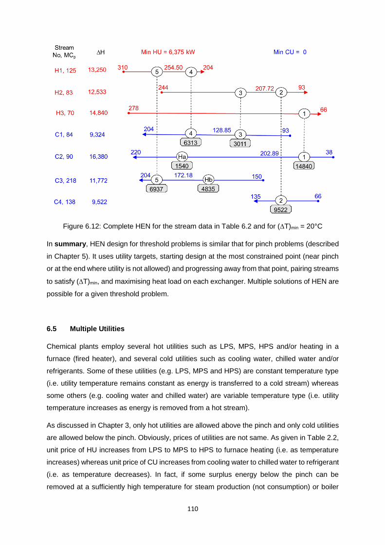
110
Figure 6.12: Complete HEN for the stream data in Table 6.2 and for (T)min = 20°C
In summary, HEN design for threshold problems is similar that for pinch problems (described
in Chapter 5). It uses utility targets, starting design at the most constrained point (near pinch
or at the end where utility is not allowed) and progressing away from that point, pairing streams
to satisfy (T)min, and maximising heat load on each exchanger. Multiple solutions of HEN are
possible for a given threshold problem.
6.5 Multiple Utilities
Chemical plants employ several hot utilities such as LPS, MPS, HPS and/or heating in a
furnace (fired heater), and several cold utilities such as cooling water, chilled water and/or
refrigerants. Some of these utilities (e.g. LPS, MPS and HPS) are constant temperature type
(i.e. utility temperature remains constant as energy is transferred to a cold stream) whereas
some others (e.g. cooling water and chilled water) are variable temperature type (i.e. utility
temperature increases as energy is removed from a hot stream).
As discussed in Chapter 3, only hot utilities are allowed above the pinch and only cold utilities
are allowed below the pinch. Obviously, prices of utilities are not same. As given in Table 2.2,
unit price of HU increases from LPS to MPS to HPS to furnace heating (i.e. as temperature
increases) whereas unit price of CU increases from cooling water to chilled water to refrigerant
(i.e. as temperature decreases). In fact, if some surplus energy below the pinch can be
removed at a sufficiently high temperature for steam production (not consumption) or boiler

111
feed water heating, then it can result in credit (i.e. revenue) instead of cost. Therefore, the use
of available utilities in the plant should be optimised for cost reduction, which also contributes
to reducing fuel used in the plant.
GCC can be used to choose and optimise the use of utilities available in the plant. Obviously,
cheaper utilities should be used as much as possible. This will decrease operating cost but,
as will be seen later, it will also increase number of units and capital cost. For the example
problem and (∆T)min = 10°C, whose GCC is given in Figure 6.1, HU target is 3.86 MW. For
this, should we use steam at 215°C (denoted as IPS from now on) given in Table 4.1 alone or
along with LPS at 160°C? And, how much of each of them should be used? Answers to these
questions can be found from GCC.
Noting (∆T)min = 10°C and HU is equivalent to a hot stream, shifted temperatures
corresponding to steam temperatures of 160°C and 215°C are 155°C and 210°C, respectively.
Figure 6.13 show LPS and IPS as horizontal lines at shifted temperatures of 155°C and 210°C,
respectively; IPS is the red dashed line at the top whereas LPS is the dark red dashed line
closer to the pinch. Both these are above the pinch and hence they can be used as HUs in
the example problem. Specifically, IPS line is well above GCC, and so it can be used to supply
the entire HU target of 3.86 MW.
Alternately, can we use the cheaper LPS to provide the entire HU target of 3.86 MW? LPS
line is crossing GCC; this means some of the enthalpy deficit (i.e. HU requirement) is above
LPS temperature, and so it cannot be satisfied by LPS (because of negative temperature
driving force). In other words, LPS can be used until its line from y-axis touches GCC, which
is shown by diamond symbol in Figure 6.13. Net heat flow at this point can be read
approximately from the plot or calculated accurately by interpolation of the relevant segment
of GCC (i.e. straight line of GCC passing through this point). Thus, LPS up to 2.6 MW can be
used. Since HU target (3.86 MW) is more than this, rest of HU required (= 3.86 – 2.6 = 1.26
MW) will have to be supplied by the relatively more expensive IPS.

112
Figure 6.13: GCC with two hot utilities: IPS and LPS
In summary, two possibilities of supplying HU target are: (i) use IPS of 3.86 MW, and (ii) use
LPS of 2.6 MW and IPS of 1.26 MW. Since IPS is more expensive than LPS, operating cost
of using LPS and IPS combination (shown in Figure 6.14) will be lower than that of using IPS
totally. Is there any adverse effect of using LPS and IPS combination on capital cost? Indeed,
capital cost will be more. Reasons are elaborated below with reference to Figure 6.14.
Figure 6.14: GCC with HU target satisfied by LPS (2.6 MW) and IPS (1.26 MW)
IPS
LPS
Utility Pinch
Process Pinch

113
IPS of 1.26 MW satisfies energy deficit of cold streams (after transfer of energy from hot
streams) in the shifted temperature range from 195°C to 155°C. LPS of 2.6 MW meets the
energy deficit of cold streams in the shifted temperature range from 155°C to 95°C (pinch).
This means, net heat flow immediately above 155°C (i.e. 155+) is zero, and temperature
driving force between LPS and cold stream(s) at 155°C is (∆T)min (= 10°C). Both these imply
there is a pinch whenever the utility line touches GCC. In case LPS used is less than 2.6 MW
(say, 2.4 MW), then the utility line does not touch GCC and there is no pinch at 155°C.
Pinch formed by touching of the utility line with GCC is referred to as utility pinch whereas the
pinch described in Chapter 4 is known as process pinch since it is due to the set of process
streams involved. Significance of both pinches is the same. Similar to process pinch, utility
pinch divides HEN design above the process pinch (at 95°C in Figure 6.14) into two sub-
problems: above and below utility pinch (besides the sub-problem before the process pinch).
Temperature driving force for heat transfer near utility pinch will be at or slightly more than
(∆T)min. Further, utility pinch often increases number of units. HEN design above and below
utility pinch is similar to that above and below process pinch. This is described in the next
section.
Vertical distance between utility lines and GCC in Figure 6.13 is more than that in Figure 6.14.
This indicates driving force for heat transfer will be more and HEN design will be relatively
easier if only IPS (single utility) is used. Hence, use of two utilities (LPS and IPS in the
example) may lead to a utility pinch, more number of units, lower driving forces for heat transfer
and complex HEN, all of which increase capital cost. Operating cost decrease from use of two
utilities often outweighs capital cost increase. Hence, use of multiple utilities should be
investigated for potential total cost reduction.
Generally, different levels of steam are used for several reasons: (1) steam generation is more
efficient at high pressure; (2) site power generation is possible; (3) some of the critical or large
equipment are driven by steam turbines; which naturally makes steam available at different
levels; (4) using very high pressure and temperature steam for colder services makes
equipment design difficult and increases capital cost; and (5) some process streams are not
tolerant to extreme temperatures.
Instead of IPS and LPS, consider flue gas at, say, 225°C (or shifted temperature of 220°C)
from a furnace. This assumed flue gas temperature is well above pinch and GCC also, and so
it can be used as HU. The 3 straight lines in Figure 6.15 correspond to different options for
using flue gas available at 225°C. Slope of each straight line is equal to reciprocal of MCp of
flue gas. As heat is transferred from flue gas to cold streams, flue gas temperature decreases;
this decrease is more if MCp (i.e. flow rate) of flue gas is low, and vice versa.

114
First option for flue gas use in Figure 6.15 is the continuous red line, which is well above GCC
and pinch, and so it is feasible. Here, the line is inclined since flue gas is a variable temperature
utility, whose temperature decreases as it supplies heat to the process stream. On the other
hand, steam is a constant temperature utility and so its line is horizontal, i.e. parallel to x-axis,
as in Figure 6.14. Second option is dashed red line touching (but not crossing) GCC at pinch;
this is also feasible but driving force for heat transfer is less than that in the first option. The
third option is the black dotted line crossing GCC and so it is not feasible. In other words, a
utility (flue gas) line just touching (at any point) or above GCC is feasible.
Figure 6.15: GCC with three options (shown by straight lines) for using flue gas at 225°C to
provide HU target
If the utility line touches, then there will be a utility pinch, lower driving force for heat transfer
and higher capital cost but operating cost will be lower since flue gas flow rate (MCp) will be
lower. On the other hand, if the utility line is above GCC, there will be no utility pinch, higher
driving force and lower capital cost but operating cost will be higher since flue gas flow rate
will be more. Note that flue gas line depends on its starting temperature and flow rate, and
they in turn affect operating and capital costs. Final choices for flue gas temperature and flow
rate depend on availability in the plant and economics. Note that final flue gas temperature is
also limited by acid dew point, and hence slope of the line will be limited.
Another common hot utility in industry is hot oil, which is used in a closed circuit (i.e. hot oil is
obtained from a furnace, used for heating in the process and then returned to the furnace for
re-heating). Maximum temperature of hot oil depends on its material. Similar to flue gas, hot

115
oil temperature decreases when it is used for heating in the process. Hence, flue gas and hot
oil are variable temperature utilities. Hot oil temperature change during heating of a process
stream can be represented as an inclined straight line (similar to flue gas lines in Figure 6.15).
Energy balance can be used to find the required MCp of flue gas or hot oil. Consider the flue
gas usage from 225oC (shifted T of 220oC) to 100oC (shifted T of 95oC at the pinch), which is
shown by dashed red line in Figure 6.15. As stated, this is feasible and required lower MCp.
This flue gas has to supply the entire HU requirement of 3.86 MW. By energy balance,
MCp of flue gas = 3.86 / (225 – 100) = 0.03088 MW/oC = 30.88 kW/oC (6.1)
Heat capacity (specific heat) of flue gas depends on its composition and temperature. For
example, it can vary from 1.1 to 1.3 kJ/(kg.oC). Taking an average value of 1.2 kJ/(kg.oC),
mass flow rate of flue gas is 30.88 /1.2 = 25.73 kg/s. This is the minimum flow rate of flue gas
for the example data in Figure 6.15. If it is lower than this minimum, flue gas line crosses GCC
(black dotted line in Figure 6.15), which is not feasible.
Now, let’s turn our attention to CU requirement below the process pinch. See the ‘pocket’ or
triangle in Figure 6.16 formed by GCC and the added dashed vertical line. This is because of
enthalpy deficit in the interval from 45°C to 35°C. It is best to satisfy this deficit by excess
enthalpy in the interval(s) just above it. In other words, heat exchange in the pocket is between
hot and cold streams, and no utility (CU in case the pocket is below pinch and HU in case the
pocket is above pinch) is allowed inside the pocket.
CU for the example problem is cooling water from 30°C to 45°C in Table 4.1. It is represented
by the dashed blue line from shifted temperature of 35°C to 50°C in Figure 6.16.28 Referring
to the table in Figure 6.1, energy removed by cooling water is 1.52 MW or 1,520 kW. If
required, cooling water flow rate can be found using Equation 1.4. Cooling water line touches
GCC at 30°C, as shown in Figure 6.16, and so temperature driving force will be at a minimum
and net heat flow will be zero at this point. This leads to a utility pinch at 30°C but its effect on
HEN design is not much as it is at one end of GCC.
28 Note that CU is equivalent to a cold stream.

116
Figure 6.16: GCC below pinch with two options: cooling water (blue dashed line) and boiler
feed water (blue thin line), for satisfying CU target of 1.52 MW below pinch
Since energy to be removed is from pinch at 95°C to 60°C in Figure 6.16, it is possible to
use this energy to pre-heat boiler feed water from 55°C (shifted temperature of 60°C) to, say,
85°C (shifted temperature of 90°C), instead of cooling water from 30°C to 45°C. This alternate
of using boiler feed water is shown by blue thin line in Figure 6.16. Boiler feed water line
touches GCC at 60°C, and so temperature driving force will be minimum and net het flow will
be zero at this point. This leads to a utility pinch at 60°C, which affects HEN design since there
are streams above and below it.
What are the relative merits of using cooling water or boiler feed water as CU in Figure 6.16?
Cooling water usage incurs operating cost but temperature driving force below pinch will be
relatively more leading to smaller exchangers/coolers and lower capital cost. On the other
hand, boiler feed water usage does not incur operating cost and even save energy used for
pre-heating boiler feed water but there will be a utility pinch and temperature driving force will
be just above (∆T)min leading to more units, larger exchangers/coolers and consequently
higher capital cost. Hence, economics of using energy removed from process streams should
be explored in industrial applications.GCC for another set of streams (see Exercise 6.1 at the
end of this chapter) is shown in Figure 6.17. Here, (T)min = 20°C, pinch is at shifted
temperature of 250°C (260/240°C), minimum HU is 5,940 kW, minimum CU is 8,440 kW and
GCC has pcokets above and below pinch. Since pinch temperature is high, it is possible to
use surplus energy below pinch for steam production. This is shown in Figure 6.17 by CU line
at shifted temperature of 135°C; note that this line does not go into the pocket and so surplus
energy to be removed is 8,440 kW. Assuming boiler feed water is available at 125°C and
Boiler Feed
Water
Cooling
Water

117
noting latent heat of vaporisation of water at this temperature is 2,188 kJ/kg, this surplus
energy can produce 8,440/2,188 = 3.857 kg/s of steam at 125°C.
Figure 6.17: GCC with pockets above and below pinch, and use of CU for steam production
at shifted temperature of 135°C
Referring to Figure 6.17, steam production at 125°C (shifted temperature of 135°C) will result
in zero net heat flow and a utility pinch at shifted temperature of 75°C (and not at 135°C). This
utility pinch is not important in HEN design as there are no process streams below it. In fact,
same amount of steam can be produced at temperature more than 125°C until 198°C (shifted
temperature of 208°C, where the vertical black line touches GCC). If steam is produced (i.e.
CU is used) at 198°C, there will be zero net heat flow and two utility pinches at shifted
temperatures of 208°C and 75°C. Of these, utility pinch at the higher temperature affects HEN
design because of streams above and below it.
6.6 HEN Design for Multiple Utilities
In the previous section, use of two utilities (namely, IPS and LPS) is discussed for the stream
data in Table 3.4 for the example employed in Chapter 3; see GCC in Figure 6.14 and the
related discussion in the previous section. HU target of 3.86 MW can be provided by 2.6 MW
of LPS and 1.26 MW of IPS, which will result in a utility pinch at 155°C (160/150°C). To begin

118
HEN design for this case of two hot utilities, stream data, enthalpy changes and targets are
compiled in Figure 6.18, which has more data compared to grid diagrams in Chapter 5, as
follows. First, enthalpy change is given for 3 zones: above utility pinch, between utility and
process pinches, and below process pinch. Second, there are two pinches: utility and process
pinches. Third, LPS is shown at the top of hot streams, its temperature remains unchanged at
160°C and so its MCp is infinity; this is to facilitate HEN design between two pinches whereas
IPS (used above the utility pinch) is not shown for simplicity.
Figure 6.18: Grid diagram showing stream data, enthalpy changes and targets for using two
hot utilities; enthalpy changes and utilities are in kW
Since the 3 zones are separate sub-problems, HEN in each of them can be designed
independent of each other. Here, HEN is designed starting from below the process pinch, then
between process and utility pinches, and finally above the utility pinch. Each of them follows
the procedure used in Chapter 5 (i.e. design starting from pinch and then progressing away,
satisfying golden rules, pinch matches meeting MCp criterion and maximising heat load on
each match). HEN design below the process pinch is same as that in Chapter 5; see this in
Figure 6.19 and compare it with that in Figure 5.2.
For HEN design between two pinches, MCp criterion for pinch matches above a pinch is
opposite to that for pinch matches below a pinch (Equation 5.4 versus Equation 5.5). In other
words, the two are conflicting. Common-sense approach is employed for satisfying applicable
MCp criterion. For this, list all feasible pinch matches between utility and process pinches; in
Figure 6.17, they are as follows.
Above Process Pinch: H1 with C2; and H2 with C3

119
Below Utility Pinch: H1 with C1; LPS with C1; and LPS with C2
In the above, there is choice for pairing LPS with either C1 or C2, and all other pairings are
compulsory. Hence, first pair those streams where there is no choice. These are H1 with C2
(match 3) and H2 with C3 (match 4) in Figure 6.19; their duties are selected to satisfy enthalpy
changes of streams H1 and H2, respectively. Since H1 requirement is fully met by match 3,
LPS is paired with C2 below utility pinch (match 5). Instead of pairing H1 with C2 above
process pinch, match of H1 with C1 below utility pinch can be chosen. Then, a slightly different
HEN will be obtained between utility and process pinches. Readers are urged to develop this.
Figure 6.19: HEN for multiple utilities: after design below process pinch and some matches
between utility and pinch matches
The remaining design problem between pinches in Figure 6.19 is heating of C1 from its supply
temperature to utility pinch, heating of C3 from 112.94°C to its target temperature, and LPS
can be used where required. Readers are asked to think about the matches needed to satisfy
these as well as HEN design above the utility pinch before seeing the complete HEN in Figure
6.20. Further, in this figure, verify all calculated temperatures with two decimal digits and
hot/cold utilities used against their targets.

120
Figure 6.20: Complete HEN design for multiple utilities
Does the complete HEN in Figure 6.20 use minimum number of units in each zone? Minimum
number of units by Equation 4.3 is as follows:
Above Utility Pinch: 4 – 1 = 3
Between Utility and Process Pinches: 6 – 1 = 5
Below Process Pinch: 4 – 1 = 3
Clearly, HEN in Figure 6.19 is using the minimum number units for each sub-problem.
If there is no utility pinch but still using some LPS (i.e. less than the target of 2,600 kW),
minimum number units above process pinch is 6 (= 5 process streams + 2 hot utilities – 1),
which is 2 units less than the design in Figure 6.20. One possible solution with no utility pinch
and LPS < 2,600 kW is shown in Figure 6.21. To obtain this solution from Figure 6.20, match
5 duty is transferred to heater Hb and match 8 duty is combined with that of match 3, thus
matches 5 and 8 are eliminated.
In the HEN in Figure 6.21, check calculated temperatures, approach temperatures satisfying
(∆T)min = 10°C and total HU against target. In this alternate solution, LPS used is 2,060 kW
(instead of maximum possible 2,600 kW) but the advantage is 2 fewer units and so lower
capital cost. Again, total annual cost and operability should be considered to choose the
solution in Figure 6.20 or Figure 6.21.

121
Figure 6.21: HEN using two hot utilities but without utility pinch
6.7 Summary
This chapter describes GCC, threshold problems and multiple cold/hot utilities. GCC is a plot
of shifted temperature versus net heat flow in the feasible heat cascade, and it is useful for
analysing threshold problems and finding hot/cold utilities that can be used. Threshold
problems require only one utility (either HU or Cu) and the minimum utility remains constant
(i.e. does not vary with (∆T)min) until certain threshold value. Minimum temperature difference
for heat transfer among process streams can occur between the two ends of composite curves
(first type of threshold problems) or at one end of composite curves (second type of threshold
problems).
Use of more than one cold or hot utility leads to a utility pinch; this is in addition to a process
pinch. It can reduce operating cost at the expense of some increase in capital cost for HEN.
HEN design procedure described in Chapter 5 can be adopted for designing HEN for both
types of threshold problems and for the use of multiple utilities. This is described with the help
of several examples in Sections 6.4 and 6.6. For alternate description and solved exercises
on threshold problems, use of multiple utilities and HEN design for them, see Sections 3.3,
3.4, 4.5 and 4.6 in Kemp (2007) and/or Sections 16.3, 16.7, 18.3 and 18.4 in Smith (2005).

122
6.8 References
Kemp I.C., Pinch Analysis and Process Integration: A User Guide on Process Integration for
Efficient Use of Energy, 2nd Edition, Butterworth-Heinemann (2007).
Smith R., Chemical Process Design and Integration, John Wiley (2005).
6.9 Exercises
1. A chemical process has the following streams.
Stream Supply
Temperature (°C)
Target
Temperature (°C)
Flow Rate Heat
Capacity (kW/°C)
S1 350 115 95
S2 260 150 312
S3 65 310 207
S4 100 170 49
It is proposed to produce steam from the excess heat in the above process streams.
Analysis for (T)min = 20°C gave the following heat cascade results.
Shifted
Temperature (°C)
Heat Cascade
(kW)
340 5940
320 7840
250 0
180 14000
140 20040
110 15210
105 14650
75 8440
Two steam pressures with saturation temperatures of 215°C and 125°C, are available
for steam production in the plant. How much steam (in kW and kg/s) can be produced
at each of these temperatures? Assume that only one type of steam is produced at a
time and boiler feed water is available in liquid phase at saturation temperature. Hint:
recall that the utility line should not go into the pocket and obtain the required latent heat
of vaporisation from steam tables or internet.

123
2. For the stream data in Table 3.1 and (∆T)min = 20°C, minimum utilities, energy recovered
and pinch were found in Exercise 3.2, and Umin, MER was found in Exercise 4.5. Prepare
GCC for this set of stream data and (∆T)min = 20°C. Is LPS at 160°C alone sufficient to
provide the entire HU target? If not, how much LPS can be used and how much HPS at
254°C is required? State the utility pinches, if any, resulting from the use of LPS.
3. As a continuation of Exercise 6.1, value of steam that can be produced at the higher
pressure (i.e. saturation temperature) is 1.4 times that of steam at the lower pressure
(i.e. saturation temperature). For maximum revenue, what pressure steam (only one)
should be produced and how much? For this, develop a HEN meeting the targets.
4. As a continuation of Exercise 6.2, design HEN for the use of LPS and HPS combination
to satisfy the HU target.
5. A petroleum refining process has streams given in the following table. These streams
can be considered for energy recovery and reuse among them. For a minimum driving
force of 15°C, minimum hot utility is zero and cold utility is 18.56 MW. Design a HEN
using minimum utilities (i.e. for maximum energy recovery). Is the HEN designed using
the minimum number of units or more number of units?
Stream Number
and Name
Supply
Temperature (°C)
Target
Temperature (°C)
Flow rate Heat
Capacity (MW/°C)
S1: Feed-1 38 121 0.443
S2: Feed-2 121 193 0.517
S3: Feed-3 193 282 0.527
S4: Reflux-1 127 71 0.348
S5: Reflux-2 193 149 0.338
S6: Reflux-3 316 227 0.469
S7: Kerosene 160 110 0.105
S8: Diesel 271 143 0.116
S9: Residue 354 149 0.211
6. Study the following statements carefully and choose the correct statement.
(A) In the plot of grand composite curve, y-axis can be shifted temperature or hot
stream temperature or cold stream temperature.
(B) In the plot of composite curves, minimum temperature difference can occur at the
left end, between the two ends and/or at the right end.
(C) Some threshold problems have near pinch, where there is some net heat flow.

124
(D) Multiple utilities refer to use of more than one type of cold utility.
(E) In case of utility pinch, there will more sub-problems in HEN design.
(F) All the above statements are correct.
7. Study the following statements carefully and choose the correct statement.
(A) Grand composite curve is useful in choosing cold and hot utilities to be used.
(B) Threshold problems require either hot utility or cold utility, and not both.
(C) In case of HEN for near pinch problems, there can be a cooler above near pinch
or a heater below near pinch.
(D) Utility pinch occurs whenever the utility line touches GCC.
(E) Multiple utilities refer to use of more than one type of hot utility.
(F) All the above statements are correct.
8. Study the following statements carefully and choose the correct statement.
(A) Grand composite curve is useful for threshold problems and not for pinch problems.
(B) Threshold problems are of only one type.
(C) In HEN design for threshold problems, MCp criterion must be satisfied for each and
every match.
(D) Multiple utilities refer to use of one cold utility and one hot utility.
(E) Utility pinch does not affect the number and size of units.
(F) All the above statements are wrong.
9. Study the following statements carefully and choose the correct statement.
(A) Grand composite curve does not show process pinch even if it is present.
(B) In threshold problems, utility target increases with (∆T)min.
(C) HEN design for threshold problems is very different from that for pinch problems.
(D) Utility pinch has no effect on capital cost.
(E) MCp criterion below the utility pinch is the same as that above the process pinch.
(F) All the above statements are wrong.

125
Chapter 7
Pinch Analysis: Design via Stream Splitting and Cyclic Matching
By
Gade Pandu Rangaiah
7.1 Overview
Recall heat exchanger network (HEN) design described in Chapter 5. There, the design uses
grid representation, golden rules, definition of a pinch match and MCp criterion for pinch
matches. Many of these are also employed in Chapter 6 for HEN design of threshold problems
and for design between two pinch points. Although the concepts and procedures used in
Chapters 5 and 6 are effective, they are not sufficient for HEN design of all problems
encountered in industrial practice.
In this chapter, the concept of splitting a cold or hot stream into two or more (sub-)streams or
branches for HEN design is introduced and illustrated in Sections 7.2 and 7.3. This also brings
another criterion, known as number criterion (similar to MCp criterion) for pinch matches. Note
that stream splitting into two or more (sub-)streams is possible and used in industrial practice.
Algorithm for stream splitting is described in Section 7.4. With stream splitting, HEN design of
any problem (i.e. any number of cold/hot streams, (∆T)min, and pinch or threshold type) using
minimum number of units (found by the equation described in Chapter 4) is possible.
In case stream splitting is not allowed or possible, the alternate strategy is cyclic matching,
which is introduced and illustrated in Section 7.5. The drawback of cyclic matching is the need
for more units than the minimum target. HEN design away from the pinch is outlined in Section
7.6. Finally, contents of this chapter are summarised in Section 7.7.
The learning outcomes of this chapter on HEN design via stream splitting and cyclic matching,
are as follows:
1. Describe stream splitting and the need for it
2. Explain number criterion and the need for it
3. Apply stream splitting to HEN design
4. Describe cyclic matching
5. Design HEN with cyclic matching
6. Perform HEN design away from the pinch

126
7.2 Stream Splitting and Number Criterion
Stream splitting refers to splitting or dividing a cold (or hot) stream into two or more (sub-
)streams or branches for heat exchange with hot (or cold) streams for designing a feasible
HEN.29 After heat exchange, split streams will be mixed, and there will be only one cold (or
hot) stream, which may need further heating (or cooling). In other words, stream splitting will
not affect the streams leaving HEN (i.e. after heat integration in HEN). Stream splitting requires
additional piping and instrumentation for implementing and maintaining the desired split
ratio/fraction, and hence additional capital and operating costs. However, these additional
costs are not substantial and stream splitting, where required, is practiced in industries.
Considering the additional costs, why is stream splitting required? Reason for stream splitting
at the pinch can be one or both of the following:
(i) streams at the pinch do not satisfy MCp criterion for feasible pinch matches30
(ii) number of cold (or hot) streams at the pinch is not sufficient for pinch matches above (or
below) the pinch
Stream splitting may also be required for matching streams away from the pinch. Let’s
understand each of the above reasons with a suitable example.
Consider the stream data from the process flowsheet given earlier in Exercise 3.3 These data
along with the targets found for (∆T)min = 20°C are presented in the grid diagram in Figure 7.1.
HEN design above pinch is simple as there are only two cold streams and no hot stream. It
requires two heaters, as shown in Figure 7.1.
Below pinch, there are two cold streams that have to be heated to pinch temperature (160°C)
using only hot streams since HU cannot be used. However, there is only one hot stream
(namely, Effluent), which by itself is not sufficient to heat two cold streams. This leads to the
following number criterion, similar to MCp criterion, for feasible pinch matches.
nh ≤ nc for above pinch (7.1)
nh ≥ nc for below pinch (7.2)
Here, nh and nc are respectively the number of hot and cold streams at the pinch. In counting
nh and nc, only the hot/cold streams at the pinch (i.e. involving pinch temperature) are
29 In this and other sentences, the alternate possibility is given in brackets.
30 A pinch match refers to the exchanger having both hot and cold stream temperatures on left or right
side of the match equal to pinch temperatures. Revisit Chapter 5 for more details.

127
considered whereas hot/cold streams away from the pinch must be excluded. For example,
C1 stream in Figure 7.5 (given later) is not counted in nc for above pinch.
Figure 7.1: Stream data and HEN above pinch for the process flowsheet in Exercise 3.3
In the problem in Figure 7.1, Equation 7.2 is not satisfied below pinch. Therefore, the single
hot stream is split into two branches or (sub-)streams for matching with the two cold streams.
How should the hot (Effluent) stream be split – equally or some other ratio? There are many
feasible solutions to this splitting. However, stream splitting should satisfy MCp criterion for all
required pinch matches. One suggestion is to split the hot (cold) stream in proportion to MCp
of cold (hot) streams involved, which provides more uniform driving forces in the HEN.
In the example (Figure 7.1), MCp of the two cold streams is 3 kW/°C and 2 kW/°C; hence, the
hot (Effluent) steam with MCp of 6 kW/°C is split into two branches having MCp of 63/(3+2) =
3.6 kW/°C and 62/(3+2) = 2.4 kW/°C; these MCp values are shown inside the ‘chord’ box
near each branch stream in Figure 7.2. Now, the two branch or (sub-)streams can be matched
with the two cold streams satisfying MCp criterion for pinch matches, as shown in Figure 7.2.
As in Chapter 5, duty of matches 1 and 2 is maximised, and the temperature of each branch
stream after each match is calculated away from the pinch temperature towards the right (i.e.
decreasing temperature). Confirm duties of matches 1 and 2 as well as calculated
temperatures in Figure 7.2.
The two branch streams after heat exchange in matches 1 and 2 are at 67.5°C and 80°C.
They are now mixed to obtain the original Effluent stream, and its temperature is calculated
by energy balance at the mixing point (adiabatic without any heat loss). This temperature can
be obtained from the following equation arising from energy balance:
T (after mixing) = 3.6×67.5 + 2.4×80
3.6 + 2.4 = 72.5°C (7.3)

128
The hot Effluent stream has to be cooled subsequently from 72.5°C to its target temperature
of 40°C using CU in a cooler. Complete HEN with stream splitting below pinch for the stream
data in the process flowsheet in Exercise 3.3, is in Figure 7.3.
Figure 7.2: Stream splitting below pinch and matching of split/hot streams with cold streams
Figure 7.3: HEN with stream splitting below pinch for the stream data in the process
flowsheet in Exercise 3.3
It is very important to note that the target for minimum number of units (Equations 4.2 to 4.4)
is based on the original number of streams (i.e. without counting split branches). For example,
in Figure 7.3, Umin, below = 1 hot stream + 2 cold streams + 1 cold utility – 1 = 3. Despite stream
splitting for the purpose of matching, HEN design below pinch in Figure 7.3 meets this target
on number of units.
Another HEN design for the stream data in the process flowsheet in Exercise 3 is given in
Figure 7.4. Reader is urged to check this design, which is based on splitting the Effluent stream

129
(MCp = 6 kW/°C) into two branches with the same MCp (= 3 kW/°C). The right-side approach
temperature31 of matches 1 and 2 are respectively 20°C and 60°C, which are significantly
different. On the other hand, they are 42.5°C and 40°C in the HEN design in Figure 7.3, which
are comparable and likely to require less heat transfer area for matches 1 and 2 together
compared to the matches 1 and 2 in Figure 7.4. Hence, it is better to split the hot (cold) stream
in proportion to MCp of cold (hot) streams involved, which provides more uniform driving forces
in the HEN. However, stream splitting in any fraction is acceptable as long as it can lead to
feasible pinch matches.
Figure 7.4: HEN with stream splitting below pinch for the stream data in the process
flowsheet in Exercise 3.3: design for the case of splitting the Effluent stream into two
branches with equal MCp
7.3 Stream Splitting for Satisfying MCp Criterion
As mentioned in the previous section, stream splitting may be required for meeting MCp
criterion for the required pinch matches. This is illustrated for HEN design of stream data in
Table 7.1, which are very similar to that considered earlier in Table 3.1. The only difference is
the increase in MCp of H1 stream from 73 kW/K to 86 kW/K. Targets for the stream data in
Table 7.1 and (∆T)min = 10°C, are minimum HU of 2560 kW, minimum CU of 2170 kW and
pinch at 100/90°C. Grid diagram with HEN design below pinch is presented in Figure 7.5.
Reader is urged to confirm the below-pinch design in this figure.
31 Recall from Chapter 2 that approach temperature is the difference in temperatures of hot and cold
streams on one side of a heat exchanger.

130
Table 7.1: Stream data for illustrating stream splitting: modified value (compared to those in
Table 3.1) is identified in red colour
Stream Type TS (°C) TT (°C) MCp (kW/K) Enthalpy Change (kW)
H1 Hot 200 50 86 -12,900
H2 Hot 140 50 39 -3,510
C1 Cold 130 170 45 +1,800
C2 Cold 90 190 82 +8,200
C3 Cold 30 130 68 +6,800
Figure 7.5: Grid diagram with HEN below pinch for the stream data in Table 7.1
For pinch matches above pinch, there are 2 hot streams (H1 and H2) and 2 cold streams (C2
and C3); C1 stream is not counted as it is away from pinch temperature (i.e. its supply
temperature of 130°C is higher than pinch temperature of 90°C). Thus, number criterion
(Equation 7.1) is satisfied. Matching of H2 with C2 or C3 satisfies MCp criterion of MCp,h ≤
MCp,c (Equation 5.4), and so H2 can be cooled to pinch temperature using either C2 or C3.
Next, can H1 with MCp of 86 kW/K be paired with C2 (MCp = 82 kW/K) or C3 (MCp = 68 kW/K)
for cooling H1 to pinch temperature? Both these pairings violate MCp criterion.
In order to satisfy MCp criterion, H1 stream has to be split into 2 (sub-)streams, to reduce its
MCp.32 This results in 3 hot streams, namely, 2 branches of H1 and H2, and violates number
of criterion (Equation 7.1) since there are only 2 cold streams for pinch matches. Therefore,
32 Note that MCp of any stream cannot be increased since mixing of given streams is not allowed.
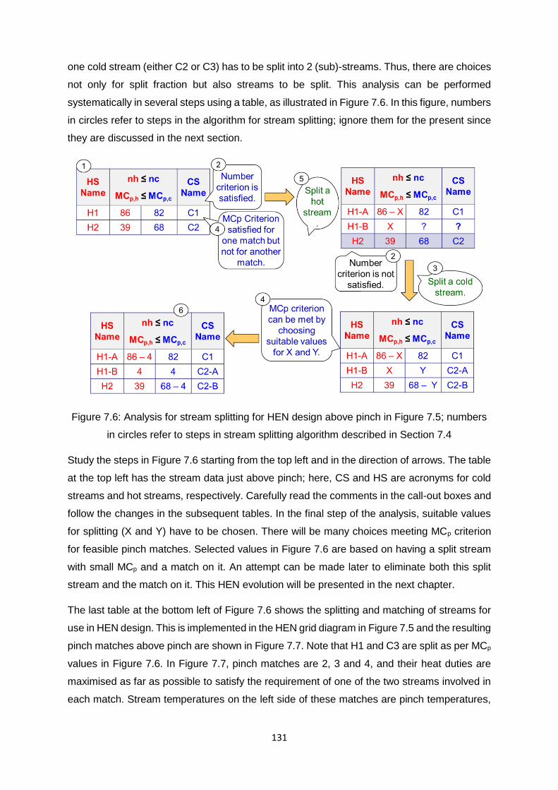
131
one cold stream (either C2 or C3) has to be split into 2 (sub)-streams. Thus, there are choices
not only for split fraction but also streams to be split. This analysis can be performed
systematically in several steps using a table, as illustrated in Figure 7.6. In this figure, numbers
in circles refer to steps in the algorithm for stream splitting; ignore them for the present since
they are discussed in the next section.
Figure 7.6: Analysis for stream splitting for HEN design above pinch in Figure 7.5; numbers
in circles refer to steps in stream splitting algorithm described in Section 7.4
Study the steps in Figure 7.6 starting from the top left and in the direction of arrows. The table
at the top left has the stream data just above pinch; here, CS and HS are acronyms for cold
streams and hot streams, respectively. Carefully read the comments in the call-out boxes and
follow the changes in the subsequent tables. In the final step of the analysis, suitable values
for splitting (X and Y) have to be chosen. There will be many choices meeting MCp criterion
for feasible pinch matches. Selected values in Figure 7.6 are based on having a split stream
with small MCp and a match on it. An attempt can be made later to eliminate both this split
stream and the match on it. This HEN evolution will be presented in the next chapter.
The last table at the bottom left of Figure 7.6 shows the splitting and matching of streams for
use in HEN design. This is implemented in the HEN grid diagram in Figure 7.5 and the resulting
pinch matches above pinch are shown in Figure 7.7. Note that H1 and C3 are split as per MCp
values in Figure 7.6. In Figure 7.7, pinch matches are 2, 3 and 4, and their heat duties are
maximised as far as possible to satisfy the requirement of one of the two streams involved in
each match. Stream temperatures on the left side of these matches are pinch temperatures,

132
and stream temperatures on the right side are calculated (i.e. stream temperatures are
calculated away from the pinch and are higher). The two branch streams of C3 on the right
side of matches 3 and 4 are at different temperatures (namely, 114.38°C and 130°C); they are
mixed and the resulting mixed stream is at 115.3°C.
Figure 7.7: Stream splitting and pinch matches above pinch, and HEN below pinch for the
stream data in Table 7.1
The remaining problem above pinch in Figure 7.7 is (i) cooling of H1 branch with MCp of 4
kW/K from 200°C to 140°C, (ii) heating of C1 from 130°C to 170°C, and (iii) heating of C3
stream from 115.3°C to 130°C. These can be achieved by (i) matching H1 branch with C1, (ii)
placing one heater on C1, and (iii) placing another heater on C3, as shown in Figure 7.8.
Complete HEN in this figure satisfies minimum HU, minimum CU and Umin, below but it requires
one more unit than Umin, above target.
Is it possible to reduce the number of units above pinch? Indeed, it is possible by transferring
heat duty of match 5 (namely, 240 kW) to match 3 (on the hot stream side) and Ha (on the
cold stream side). This increases heat duty of match 3 from 160 kW to 400 kW and of Ha from
1560 kW to 1800 kW (both by 240 kW), as shown in Figure 7.9. These changes still satisfy
required enthalpy changes of H1 split branch and C1. In order to keep outlet temperature of
C3 branch from match 3 comparable to that of C3 branch from match 4, C3 split is changed –
MCp of split streams are updated to 54 and 14 in Figure 7.9 instead of 64 and 4 in Figure 7.8.
The updated HEN in Figure 7.9 meets targets for minimum utilities and minimum number of
units above and below pinch. Reader should check all temperatures (particularly, C3

133
temperatures before and after mixing), heat duty and approach temperatures of each match
above pinch in Figure 7.9.
Figure 7.8: Complete HEN with stream splitting above pinch, for stream data in Table 7.1
Figure 7.9: Improved HEN for stream data in Table 7.1: after elimination of match 5 and
adjustment of heat duties of match 3, heaters Ha and Hb as well as C3 splitting

134
Is it possible to choose the better way of C3 splitting in Figure 7.9 (which leads to fewer number
of units) earlier while doing the analysis in Figure 7.7? Indeed, it is possible with experience
and noting enthalpy changes of split streams based on their supply/target and pinch
temperatures. Alternately, one can go through two steps: develop a feasible HEN as in Figure
7.8 and then improve it to meet the target number of units as in Figure 7.9.
7.4 Algorithm for Stream Splitting
Stream splitting and its illustration in Sections 7.2 and 7.3 reveal that both number and MCp
criteria should be considered for stream splitting. Steps for stream splitting above pinch, if
required, similar to those in Figure 7.6, are as follows.
1. Collect stream data, i.e. number and MCp of cold and process streams, at the
pinch (and not those streams that are away from the pinch).
2. Check whether the number criterion (nh ≤ nc) is satisfied by the number of cold
and process streams at the pinch. (For this, split streams, if any, should also be
counted in nh and nc.) If satisfied, proceed to step 4; else, continue to the next
step.
3. Since there are more hot streams than cold streams, split a cold stream into 2 or
more (sub-)streams to satisfy the number criterion.
4. Analyse for feasible pinch matches (each satisfying MCp,h ≤ MCp,c criterion) for
cooling all hot streams (including sub-streams) to the pinch temperature using
cold streams (since no CU is allowed above pinch). If the required pinch matches
are all feasible, then proceed to step 6; else, continue to the next step.
5. Since one or more pinch matches do not satisfy MCp,h ≤ MCp,c criterion, split a hot
stream (usually with a large MCp in order to satisfy this criterion) into 2 (sub-
)streams. Proceed to Step 2 to check the number criterion since a hot stream is
split into 2 (sub-)streams.
6. Choose suitable split fraction/ratio values to satisfy MCp criterion for each of the
pinch matches.
For the stream data above pinch in Figure 7.5, application of the above steps is presented in
Figure 7.6, where numbers in circles refer to step number in the above algorithm. Note that
stream splitting and more than the required number of split branches should be avoided as
they will increase costs and complexity of HEN.
The above steps 1 to 6 are also applicable for stream splitting, if required, below pinch with
the following minor modifications: (a) number criterion should be nh ≥ nc in step 2; (b) a hot
(and not a cold) stream should be split in step 3; (c) MCp criterion should be MCp,h ≥ MCp,c in

135
step 4; and (d) a cold (and not a hot) stream should be split in step 5. With these modifications,
algorithm for stream splitting below pinch is presented in the form of flowchart in Figure 7.10.
Figure 7.10: Flowchart for stream splitting below pinch
Stream splitting algorithm in Figure 7.10 is now applied to stream data below pinch in Figure
7.1. Here, there are 2 cold streams (Feed and Recycle with MCp of 3 kW/K and 2 kW/K,
respectively) and one hot stream (Effluent with MCp of 6 kW/K). According to the first decision
box in Figure 7.10, number criterion is not met and so the hot stream has to be split into two
branches to satisfy this criterion. Then, proceeding to the second decision box in Figure 7.10,
MCp criterion can be met by choosing MCp of one branch of hot/Effluent stream between 2
and 4 kW/K (and MCp of the other branch will then be between 4 and 2 kW/K). Obviously,
there are many choices; as stated and illustrated earlier in Section 7.2, it is better to choose
MCp of branch streams proportional to MCp of (cold) streams being paired. With this, pinch
matches can be placed and the algorithm can be terminated.
7.5 Cyclic Matching
Cyclic matching of streams is a possibility for HEN design in some problems. This is illustrated
for the stream data below pinch in Figure 7.11. Here, the focus is on HEN design below pinch
and hence stream data above pinch are not shown in this figure. There are two cold streams
(C1 with MCp = 1.0 kW/K and C2 with MCp = 1.0 kW/K) and one hot stream (H1 with MCp =

136
4.0 kW/K). Note that stream data are chosen so that required duty and temperature
calculations can be performed mentally without a calculator; this facilitates understanding the
procedure and cyclic matching. For (∆T)min = 10°C, pinch is at 350/340°C and minimum cold
utility is 440 kW. Data above pinch including minimum hot utility are not required for HEN
design below pinch, and hence they are not given.
Figure 7.11: Stream data below pinch for illustrating cyclic matching
At the pinch in Figure 7.11, there is one hot stream (H1 with MCp = 2.0 kW/K) and one cold
stream (C1 with MCp = 1.0 kW/K), and C2 is away from the pinch. Hence, H1 and C1 meet
the criteria for a pinch match and can be paired for heat exchange. Using the heuristic of
maximising heat duty on a match, match 1’s heat duty is 310 kW to meet its heating
requirement, as shown in Figure 7.11, and this results in H1 outlet temperature of 272.5°C.
Remaining problem in Figure 7.11 is H1 cooling from 272.5°C to 90°C and heating of C2 from
30°C to 320°C; these have to be achieved using only CU and not HU. However, H1 at 272.5°C
cannot be used for C2 heating to 320°C. One solution is to reduce the heat duty on match 1
such that that the outlet temperature of H1 is 330°C (= 320+10 to satisfy (∆T)min = 10°C for
heating C2 to 320°C). Match 1’s heat duty is then 4(350 – 330) = 80 kW, as shown in Figure
7.12.
Remaining problem in Figure 7.12 is H1 cooling from 330°C to 90°C and heating of C1 and
C2 from 30°C to 260°C and 320°C, respectively. Of these, C2 has to be heated to 320°C
(more than 260°C for C1 heating), and should be given higher priority. So, C2 is paired with
H1 in match 2 as shown in Figure 7.13. As in case of match 1, heat duty of match 2 cannot be
maximised; it is limited by outlet temperature of H1 of 270°C (= 260+10 to satisfy (∆T)min =
10°C for heating C1 to 260°C), and corresponding match 2 heat duty is 240 kW (Figure 7.13).

137
Figure 7.12: HEN design below pinch: match 1 with H1 outlet temperature of 330°C for later
heating of C2 to 320°C
Figure 7.13: HEN design below pinch: match 2 with H1 outlet temperature of 270°C for later
heating of C1 to 260°C
Remaining problem in Figure 7.13 is H1 cooling from 270°C to 90°C and heating of C1 and
C2 from 30°C to 260°C and 80°C, respectively. Of these, heating of C1 to 260°C is priority
and so C1 is paired with H1 in match 3, as shown in Figure 7.14. Here, heat duty of match 3
can be maximised, and it is equal to energy required for C1 heating from 30°C to 260°C (=
230 kW). With this, H1 is available at 212.5°C, more than sufficient for heating C2 from 30°C
to 80°C.
Remaining problem in Figure 7.14 is H1 cooling from 212.5°C to 90°C and heating of C2 from
30°C to 80°C. This problem requires match 4 and cooler, as shown in Figure 7.15. Reader is
asked to verify duties/temperatures of these units. In Figure 7.15, observe that matches 1 and
3 involve the same cold and hot streams (namely, C1 and H1), and matches 2 and 4 involve
the same cold and hot streams (namely, C2 and H1). In other words, streams paired for
matches 1 and 2 are repeated later for matches 3 and 4 (albeit with different temperatures
and duties). This repetition of stream pairing and matches is known as cyclic matching.

138
Figure 7.14: HEN design below pinch: match 3 with maximum heat duty possible
Figure 7.15: Cyclic matching in the complete HEN design below pinch
Figure 7.16: HEN design below pinch with stream splitting and meeting target on number of
units
Minimum number of units below pinch for streams in Figure 7.15 is just 3 (= 3 process streams
+ 1 cold utility – 1). On the other hand, below-pinch HEN in this figure has 5 units. Thus, cyclic
matching leads to more units and consequently higher capital cost. In other words, target on

139
number of units will not be achieved in case of cyclic matching. Is there a way to design HEN
meeting the target on number of units? It is possible with stream splitting, as shown in Figure
7.16. Design of this HEN is similar to the example illustrated in Section 7.2, and so it is given
as an exercise at the end of this chapter.
7.6 Design Away from the Pinch
In pinch analysis, HEN design starts at the pinch and proceeds away from it. Design at the
pinch is guided by the number and MCp criteria, and it gives pinch matches. In addition to
these matches, HEN is very likely to require other units including heaters (above pinch) and
coolers (below pinch). All these have to be designed to meet the applicable (∆T)min; this is
sometimes referred to as ‘remaining problem analysis’. Although number and MCp criteria
need not be satisfied, they can also guide HEN design away from the pinch.
Design away from the pinch (or remaining problem analysis) is performed in the problems
illustrated in the earlier sections of this chapter. See (i) matches 5, Ha and Hb in Figure 7.8,
(ii) Ha and Hb in Figure 7.9, (iii) matches 2 to 4 and C in Figure 7.14, and (iv) C in Figure 7.15.
Note that stream splitting is not required for pinch matches, as in Figure 7.11. However, it
avoids cyclic matching (in Figure 7.15) and results in simpler HEN, as in Figure 7.16. One
reason for stream splitting in Figure 7.16 is because C2 target temperature of 320°C is close
to (although not at) pinch at 340°C.
7.7 Summary
Besides the golden rules and other guidelines used in Chapter 5, HEN design above and
below pinch in pinch problems, as well as HEN design in threshold problems may require
stream splitting or cyclic matching. Stream splitting is described and illustrated in Sections 7.2
and 7.3; in this context, number criterion (besides MCp criterion described in Chapter 5) and
its necessity are presented in Section 7.2. Then, an algorithm for stream splitting above pinch
(algorithm in the form of steps) and below pinch (algorithm in the form of flowchart) is
presented in Section 7.4.
Cyclic matching, which refers repeated pattern of matches between the same two streams,
may be required for HEN design away from the pinch. It leads to more units and so increases
costs. Instead of cyclic matching, stream splitting can be used to design HEN with fewer units.
In general, stream splitting is a powerful strategy that can provide a feasible HEN for almost
all problems. For alternate description and examples on stream splitting and cyclic matching,
see Section 4.3 in Kemp (2007) and/or Sections 18.3 and 18.5 in Smith (2005).

140
Recall that the number and MCp criteria for above pinch (i.e. nh ≤ nc and MCp,h ≤ MCp,c) are
different from those for below pinch (i.e. nh ≥ nc and MCp,h ≥ MCp,c) in the inequality direction.
One simple strategy to remember these is by relating them to the golden rules, i.e. only HU
above pinch (which means total energy in cooling all hot streams is less than that for heating
all cold streams) and only CU below pinch (which means total energy in cooling all hot streams
is more than that for heating all cold streams).
7.8 References
Kemp I.C., Pinch Analysis and Process Integration: A User Guide on Process Integration for
Efficient Use of Energy, 2nd Edition, Butterworth-Heinemann (2007).
Smith R., Chemical Process Design and Integration, John Wiley (2005).
7.9 Exercises
1. For the stream data below pinch in Figure 7.11, develop HEN with stream splitting. The
solution depends on split fraction; one possible solution is presented in Figure 7.15.
2. The targets for the stream data in Table 7.1 and (∆T)min = 20°C (instead of 10°C used
in Section 7.3), are: minimum HU = 3,810 kW, minimum CU = 3,420 kW and pinch at
110/90°C. What is the minimum number of units below pinch and above pinch?
Develop HEN for this problem meeting the above targets on utilities and also number
of units. The solution will be similar to the example in Section 7.3.
3. Streams and targets below pinch are given in the following diagram. How many
streams are there, what are MCp of streams, and what is (∆T)min used? Stream splitting
is not allowed for HEN design. Carry out HEN design below pinch in the grid diagram
below. Your design should not require more than the minimum CU target. Cyclic
matching can be used, if required. Does your design meet the target on number of
units? If not, how many more units than the target are present in the HEN designed?

141
4. Study each of the following statements carefully and state whether each of them is
correct/true.
(A) Stream splitting is always required for meeting the number criterion in all HEN
design problems.
(B) Stream splitting may be required for meeting the number and/or MCp criterion
during the design of HEN.
(C) Stream splitting and number of splits should be minimised as far as possible.
(D) A stream is always split into 2 branches or (sub-)streams.
(E) In some problems, cyclic matching is an alternative strategy to stream splitting.
(F) Target on minimum number of units can be met even with stream splitting.
(G) Target on minimum number of units can be met even with cyclic matching.
(H) Stream splitting may be required for designing pinch matches.
(I) Stream splitting may be required for HEN design away from the pinch.
(J) Stream splitting may be required for HEN design in the case of pinch problems
whereas it is not required in the case of threshold problems.
(K) Cyclic matching may be required for HEN design in the case of pinch problems
and also threshold problems.

142
Chapter 8
Pinch Analysis: Heat Exchanger Network Evolution
By
Gade Pandu Rangaiah
8.1 Overview
Design of a heat exchanger network (HEN) is described and illustrated for pinch problems and
threshold problems in the previous three chapters. The resulting HEN meets the target on
minimum hot and cold utilities, and achieves maximum energy recovery (MER) for the given
(∆T)min. Since almost all of the operating cost (OC) of a HEN is for hot and cold utilities, HEN
designed in the previous three chapters has the lowest OC for the chosen (∆T)min, and so it
cannot be improved in terms of OC.
HEN evolution or improvement (also referred to as HEN relaxation) is an attempt to reduce
CC by decreasing the number of units. It may increase cold and hot utilities above the target
on minimum utilities, thus relaxing the achievement of minimum utilities. This evolution
involves new concepts and procedures such as loop in a HEN, loop breaking, (∆T)min violation,
path in a HEN and (∆T)min restoration. These are described in the present chapter; HENs used
for illustration in this chapter are examples from Chapters 5 to 7.
Aim of HEN evolution is outlined in Section 8.2. Loop and loop breaking to decrease number
of units are described with examples in Sections 8.3 and 8.4. Restoration of (∆T)min, if it is
violated, using the path is presented in Section 8.5. Loop breaking and restoration of (∆T)mi
are illustrated for a slightly more complicated situation, in Section 8.6. Presentation and
illustration in Sections 8.3 to 8.6 are mostly on pinch problems with a single (process) pinch.
HEN evolution in case of threshold problems, multiple pinches and stream splitting situation
is covered in Section 8.7. Relative merits of HEN for MER and evolved HEN, and selection of
one of them are outlined in Section 8.8. Finally, contents of this chapter are summarised in
Section 8.9.
The learning outcomes of this chapter on HEN evolution are as follows:
1. Outline the purpose of HEN evolution
2. Explain a loop and a path in HEN
3. Identify and break a loop in HEN
4. Find (∆T)min violation and restore it using a path
5. Analyse HEN for MER and evolved HEN for choosing one of them

143
8.2 Purpose and Potential of HEN Evolution
HENs designed in Chapters 5 to 7 meet the target on minimum amount of cold and hot utilities
allowed for the chosen (∆T)min, and so they cannot be improved in terms of utility consumption.
OC of a HEN is mainly due to utilities,33 and so it cannot be improved too. The only possibility
for improving or evolving HENs designed in the previous three chapters is to reduce the
number of units, which affects investment (CC) required for HEN.
Consider the HEN for MER in Figure 5.2, reproduced below as Figure 8.1. In this, Umin, MER =
Umin, above + Umin, below = 5 + 3 = 8, which is more than Umin = 6 (without pinch) found in Chapter
4. This means 2 units can be reduced if pinch is not considered in this HEN design. In other
words, the difference, Umin, MER – Umin indicates the scope for reducing the number of units in
the HEN for MER and consequently CC. However, this may decrease energy recovery and
consequently increase both hot and cold utilities (by the same quantity because of energy
balance). This will be seen in the subsequent sections of this chapter.
What is the effect of decreasing the number of units on CC? Recall total heat transfer area
estimate of 5,080 m2 in Section 4.4. With the assumption of same area in each unit, area of
each exchanger is 5,080
8 = 635 m2, and installed cost of each of 8 (= Umin, MER) exchangers in
HEN is S$1,682,596 and CC of HEN is S$13,460,765 (as per Equations 4.17 and 4.18). In
case the number of units is decreased to 6 (= Umin) and total heat transfer area remains
unaffected34, area of each exchanger is then 5,080
6 = 846.7 m2, and its installed cost is:
Installed cost = 276,500 + 8,050 (846.7)0.8 = S$2,046,526 (8.1)
CC of Umin (= 6) units is
CC = 6 × 2,046,470 = S$12,279,153 (8.2)
Thus, decreasing the number of units from 8 (for HEN with pinch) to 6 (for HEN without pinch)
decreases CC from S$13,460,765 to S$12,279,153 or by 8.8%. This is the potential gain of
evolving HEN but it may be negated partially or fully or more by increase in OC due to the
increase in cold and hot utilities required. Selection between HEN for MER and evolved HEN
is discussed later in Section 8.8. Before that, let’s learn the concepts and procedures for
evolving HEN for MER, in the following sections.
33 Besides cost of utilities, other operating costs of HEN are for pumping, maintenance etc. and they are
much lower than the cost of utilities.
34 Note that the total heat transfer area is likely to change somewhat but its effect on CC is ignored for
the discussion here.

144
Figure 8.1: HEN designed for minimum utilities and minimum number of units; see Section
5.4 for details on this HEN design
8.3 Loops in a HEN
A loop in a HEN is defined as the closed route starting from certain point in the HEN and
returning back to the same point, by following streams and going through units in the HEN.
Direction of the route and of stream is not important. In other words, the closed route can be
clockwise or anti-clockwise, and a stream can be followed in the direction of its temperature
decease or increase. Study Figure 8.1 carefully and identify a loop (i.e. closed route) in Figure
8.1. Try to find the loop first and then continue reading.
One loop in the HEN in Figure 8.1 is shown in Figure 8.2; it is identified with green dashed
lines, and involves matches 2 and 4, and streams H2 and C3. The closed route in this loop
can be interpreted as follows: starting from match 4 on stream C3, one can travel up through
match 4, follow stream H2 to the right, travel down match 2 and finally follow stream C3 to the
left to the starting point. It can also be interpreted in the opposite (i.e. anti-clockwise) direction.
Further, the closed route can start at any point in the loop but it must end at the starting point.
The loop shown in Figure 8.2 is labelled as M2-M4 loop (i.e. based on matches involved in it).
There is also another loop in the HEN in Figure 8.1; compared to the loop in Figure 8.2, it is
slightly complicated and different in involving two heaters (Ha and Hb). This second loop
(Figure 8.3, wherein the three heaters are differentiated by labelling Ha, Hb and Hc) involves
matches 1 and 3, heaters Hb and Hc, and streams C2, C3 and H1 (i.e. 4 units and 3 streams).
Reader may be wondering how can one jump from one heater (Hb) to another (Hc). This is
possible because both Hb and Hc have the same hot utility stream on one side. This can be

145
seen in the HEN drawn on the balanced grid (i.e. including cold and hot utility lines), as shown
in Figure 8.4. Thus, the slightly complicated loop involves hot utility as well; in other words, it
actually involves 4 units and 4 streams including the utility stream. This loop is labelled as M1-
M3-Hb-Hc loop.
Figure 8.2: M2-M4 loop (identified by dashed green lines) in the HEN
Figure 8.3: M1-M3-Hb-Hc loop (identified by dashed green lines) in the HEN; this is in
addition to that in Figure 8.2

146
Figure 8.4: The loop shown in Figure 8.3 on the balanced grid, which includes lines for cold
and hot utilities
Generally, HEN for MER has one or more loops. Minimum number of loops35 in the HEN for
MER is given by the difference, Umin, MER – Umin, which is also the number of units than can be
eliminated (i.e. reduced in the HEN for MER). The loops can be simple (involving 2 units and
2 streams as in Figure 8.2) or complicated (involving more number of units and streams as
well as heaters and coolers, as in Figure 8.3). A loop involves even number of units and also
even number of streams (including utility streams).
8.4 Loop Breaking
A loop in a HEN provides a way to transfer some heat duty from one match to another while
meeting the heating/cooling requirements of all cold and hot streams in the HEN. Heat duty
chosen for transfer can be such that heat duty of one of the matches becomes zero, thus
eliminating that match. Usually, a match with smaller heat duty is eliminated. With the
elimination of a match, the loop under analysis is broken.
The procedure for loop breaking is illustrated on the HEN in Figure 8.1. As described in the
previous section, it has two loops (Figures 8.3 and 8.4). In this HEN, match 2 has the smallest
35 In case of two or more loops, one may identify more loops than the minimum number but each of
such loops is a combination of some or all loops already found.

147
heat duty of 430 kW. An attempt is made to eliminate this match. The M2-M4 loop shown in
Figure 8.2 (and not that in Figure 8.3) involves match 2. Heat duty for match 2 can be reduced
to zero by transferring all of it to match 4 (whose load will increase by 430 kW), as shown in
Figure 8.5. With this, cooling/heating requirements of streams H2/C3 from their supply to
target temperatures are still met. However, some intermediate temperatures of these streams
are affected. These are calculated and highlighted in Figure 8.5. Since match 2 has zero heat
duty (i.e. this match is eliminated or not required), H2 temperature before and after match 2 is
the same; this is also valid in case of C3 temperature. Note that match 1 is not in the loop, and
so its heat duty is unaffected; however, C3 inlet/outlet temperatures at match 1 are different.
Figure 8.5: HEN after breaking M2-M4 loop and updating stream temperatures (highlighted
in yellow)
Without using M2-M4 loop, heat duty of match 2 can be eliminated by transferring its heat duty
of 430 kW to cooler (on H2 side) and to heater (on C3 side). Some intermediate temperatures
of C3 and H2 will change. HEN with these changes is shown in Figure 8.6. Reader is asked
to check approach temperatures on both sides of each match; they should be at least (∆T)min
= 10°C. This way of eliminating match 2 increases utilities more than that possible by using a
loop and breaking it. Hence, it is not recommended. This is further emphasised at the end of
the next section.
8.5 Violation and Restoration of (∆T)min
After loop breaking and updating temperatures, as in Figure 8.5, approach temperatures on
both sides of each exchanger in the HEN must be checked. Is (∆T)min = 10°C satisfied by these

148
approach temperatures in the HEN in Figure 8.5? For this, Figure 8.5 without match 2 and
M2-M4 loop is shown in Figure 8.7. One approach temperature is less than (∆T)min = 10°C. It
is on the right side of match 4 with approach temperature of 88.97 – 83.68 = 5.29°C. This
means match 4 is still feasible but it will require more heat transfer area.
Figure 8.6: HEN after eliminating match 2 by transferring its heat duty of 430 kW to cooler, C
on H2 and to heater, Hc on C3
Figure 8.7: HEN without match 2 for identifying violation of (∆T)min = 10°C, if any
If (∆T)min = 10°C has to be met by all approach temperatures in the HEN in Figure 8.7, then
the violation on the right side of match 4 has to be increased from 5.29°C to 10°C. One
possibility is decreasing C3 temperature at the inlet of match 4. But this will reduce match 1

149
heat duty and also will increase H1 temperature at the exit of match 1 to above H1 target
temperature. This will then require placing a cooler on H1 stream on the right side of match 1.
In effect, number of units will increase by one and defeats the aim of HEN evolution to reduce
number of units. Hence, decreasing C3 temperature at the inlet of match 4 is not appropriate.
The other possibility is to increase H1 temperature on the right side of match 4 from 88.97°C
to 93.68°C (i.e. by 4.71°C). This will require decreasing heat duty of match 4 and increasing
duty of both cooler, C and heater Hc by the same amount = 39(93.68 – 88.97) 184 kW.
These changes are reflected in Figure 8.8. Reader should compare them with the values in
Figure 8.7. Violation of (∆T)min = 10°C on the right side of match 4 in Figure 8.7 is now restored,
and HEN in Figure 8.8 meets the requirement of (∆T)min = 10°C. This restoration of driving
force increased the utilities compared to the target.
Figure 8.8: HEN after restoration of (∆T)min = 10°C and with changes highlighted in yellow
Restoration of (∆T)min = 10°C presented in the above paragraph is possible because the
temperature that needs to be changed (i.e. H2 temperature at the exit of match 4) is on a path.
What is a path? It is an open route (and not a closed route as in a loop) from a heater, H to a
cooler, C (or from a cooler to a heater). In Figure 8.7, this path is from Hc to C via stream C3,
match 4 and stream H2. It involves one unit (excluding heater and cooler) and two streams.
Since a path is from one utility to another, it is also known as a utility path.
A path can involve more units and streams. This can be seen in Figure 6.21, which is
reproduced here as Figure 8.9.36 The paths in this figure are:
36 HEN in Figure 8.9 is used for illustrating more complicated paths later in this chapter. It has no driving
force violation. Hence, other values in this figure are not relevant for discussion of paths.

150
Ha - C1 - Match 6 – LPS - Match 7 – C3 – Match 4 – H2 – C
Hb – C2 - Match 3 – H1 – Match 1 – C3 – Match 2 – H2 – C
Each of the above two paths involves 3 matches (excluding heater and cooler) and 4 streams.
If HEN has several paths, then one of them has to be chosen for driving force restoration.
Which one should be selected? Choose the path that goes through the stream and position,
whose temperature needs to be changed for restoring (∆T)min.
Figure 8.9: HEN with two paths: one from Ha to C and another from Hb to C
Now, compare HEN in Figures 8.6 and 8.8, which are obtained by eliminating match 2 without
and with using loop, loop breaking and driving force restoration, respectively. Both HENs meet
the requirement of (∆T)min = 10°C. However, HEN in Figure 8.6 requires HU and CU of 1,590
kW and 1,950 kW, respectively; these are higher than HU and CU of 1,344 kW and 1,704 kW,
respectively, by the HEN in Figure 8.8. In terms of the expensive HU, HEN in Figure 8.6
requires 18% [= 100(1590 – 1344)/1344] more HU. Hence, follow systematic procedure using
a loop, loop breaking and driving force restoration using a path, for reducing number of units
in an effort to evolve HEN.
In some problems, however, restoration of (∆T)min may not be possible due to the absence of
an appropriate path. In such a situation, one will have to choose one of the HENs in earlier
steps (e.g. HEN for MER or HEN with some (∆T)min violation, if it is feasible).

151
8.6 Another Example of Loop Breaking and Restoration of (∆T)min
This section illustrates loop breaking and restoration of (∆T)min for a slightly more complicated
situation. Recall M1-M3-Hb-Hc loop in Figure 8.3; it is still present in the HEN in Figure 8.8
after evolution to eliminate match 2 by breaking the simpler M2-M4 loop. So, HEN in Figure
8.8 can be analysed to eliminate another match. Heater, Hb on C2 has the smallest heat duty
(of 900 kW) compared to other units in this HEN.
Heater Hb can be eliminated by reducing its heat duty by 900 kW to zero, increasing match 3
heat duty by 900 kW, decreasing match 1 heat duty by 900 kW, and finally increasing Hc heat
duty by 900 kW, as shown in Figure 8.10. Note that these changes should be performed
systematically along the loop, and they follow the alternating pattern of decrease and increase
in heat duty of a match. Furthermore, match 4 is not in the loop and so its head load is
unaffected. Some intermediate temperatures, affected by M1-M3-Hb-Hc loop breaking to
eliminate heater Hb, are highlighted and updated in Figure 8.10. Is (∆T)min = 10°C satisfied in
the evolved HEN in this figure? Look for driving force violations in Figure 8.10 before
proceeding to the next paragraph.
Figure 8.10: M1-M3-Hb-Hc loop breaking to eliminate heater Hb; heat duties and affected
temperatures are updated and highlighted in yellow
A close scrutiny of Figure 8.10 shows that approach temperature on the right side of match 3
is 87.67 – 90 = –2.33°C (i.e. negative); therefore, match 3 and consequently this HEN are
infeasible. For restoring this driving force violation, C2 temperature at the inlet of match 3 is
C2 supply temperature, and so it cannot be changed. The only option is to make H1 outlet
temperature at match 3 to 100°C. For this, is there a path from Hc to C passing through H1

152
outlet temperature at match 3? Path from heater, Ha is not possible since there is no other
match on stream C1.
Noting Hb with zero heat duty is absent now, there is no path from Hc to C passing through
H1 outlet temperature at match 3. Without a path going through it, H1 outlet temperature at
match 3 cannot be restored. Without restoring driving force violation, HEN in Figure 8.10 is
not feasible. Therefore, breaking of the second loop (i.e. further evolution of HEN in Figure
8.8) to eliminate one more unit (namely, heater, Hb) is not possible. This situation may be
encountered in some heat integration applications.
Similar to elimination of match 2 in Figure 8.6 without considering loop and loop breaking,
match 4 in Figure 8.8 can be eliminated by transferring its heat load of 1806 kW to cooler, C
and heater, Hc. However, this increases both hot and cold utilities, and consequently OC
substantially (by about 100%), and so elimination of match 4 is unlikely to be economical.
8.7 HEN Evolution in Other Situations
Recall HEN design for threshold problems and between two pinches described in Chapter 6.
Such HENs can also be analysed for improvement. In the near-pinch HEN in Figure 6.8, there
are 2 coolers: Ca and Cb. It can be improved or evolved by transferring heat duty of Cb (above
pinch) to Ca (below pinch). This is possible because of the path from Cb to Ca;37 this path is
via stream H1, match 5, stream C3, match 4 and stream H2.38 As can be seen in Figure 6.9,
heat duties of Cb, matches 5 and 4, and Ca are decreased or increased by 1050 kW, similar
to that in loop breaking. Then, affected stream temperatures are calculated. In the evolved
HEN in Figure 6.9, these changes did not lead to any driving force violation; one reason for
this is, during evolution, heat removal at a higher temperature (in Cb) is shifted to heat removal
at a lower temperature (in Ca).
For an example of evolving HEN with multiple pinches, consider the complete HEN in Figure
6.20. The focus here is on HEN above and below the utility pinch at 160/150°C. Above the
process pinch at 100/90°C, there are 8 units in total whereas the target for minimum number
of units in the absence of utility pinch is 6 (= 5 process streams + 2 hot utilities – 1). This
37 This path is slightly different in that it is from one cooler (at a higher temperature) to another cooler
(at a lower temperature).
38 An alternate path from Cb to Ca in Figure 6.8 is via stream H1, match 1, stream C3, match 2 and
stream H2. This cannot be used as match 2 heat load of 430 kW and decreasing it by 1050 kW leads
to negative heat load, which is not possible.

153
indicates the presence of 2 (= 8 – 6) loops across the utility pinch. Reader is asked to identify
them in Figure 6.20, before seeing the footnote.39
Since there are 2 loops in Figure 6.20, it is possible evolve the HEN to eliminate two units by
breaking one loop at a time (and not simultaneously). It is desirable to break the loop involving
a unit with the smallest heat duty, which is heater, Hb with duty of 360 kW. Hence, Hb should
be eliminated using the loop involving it. Accordingly, the first loop to break is Ha-M6-M5-Hb
(defined in the footnote). Procedure for breaking the 2 loops in Figure 6.20 is similar to the
description and examples in Sections 8.3 to 8.6. Hence, this is given as an exercise at the end
of this chapter.
Evolution of HENs involving stream splitting is similar to the procedures in Sections 8.3 to 8.6.
For illustration, consider the HEN in Figure 7.9, reproduced in Figure 8.11. For the stream data
in this HEN, Umin (without pinch) is 6 (5 process streams40 + one HU + one CU – 1). Since Umin,
MER = 8, the HEN has two loops; they are:
M1-M3 Loop: match 1 – stream H1 – match 3 – stream C3 (shown by thinner green
dashed lines)
Ca-M4-M3-Cb Loop: cooler Ca – stream H2 – match 4 – stream C3 – match 3 –
stream H1 – cooler Cb (shown by thicker green dashed lines)41
Thus, both loops involve match 3 and stream C3. Further, the second loop, as shown in
Figure 8.11, goes from one split stream to another on C3.
39 One loop is: match 3, stream H1, match 8 and stream C2, which is labelled M3-M8 loop. Another
loop is: Ha, stream C1, match 6, LPS, match 5, stream C2 and Hb (i.e. Ha-M6-M5-Hb loop). 40 Recall that split streams/branches must not be counted here.
41 Instead of Ca-M4-M3-Cb Loop, the second loop can be taken as Ca-M4-M1-Cb.

154
Figure 8.11: HEN with stream splitting and two loops
In the HEN in Figure 8.11, cooler, Cb has the smallest heat load of 220 kW. Hence, it is
eliminated using Ca-M4-M3-Cb Loop. For this, required changes in heat load of these units
and some intermediate temperatures are highlighted in Figure 8.12. Checking for driving force
violations show the following: (i) approach temperature of 7.44°C on the left side of match 1
and (ii) -45°C (and so infeasible) approach temperature on the right side of match 3. However,
right-side approach temperature of match 4 is increased to 15.64°C from 10°C in the HEN for
MER in Figure 8.11. How can the two violations be restored to (∆T)min = 10°C? A close scrutiny
of Figure 8.12 and noting that Cb is now absent, give that there is no path going through H1
on the right side of match 3 (i.e. the position where temperature is 45°C) from a heater (either
Ha or Hb) to cooler, Ca. Although the required path is not available, there are two possibilities
to make match 3 feasible but (∆T)min = 10°C may not be met.

155
Figure 8.12: HEN evolution – breaking of Ca-M4-M3-Cb loop to eliminate cooler, Ca with
changes highlighted in yellow
Approach temperature of 7.44°C may be acceptable since it is feasible and not far from (∆T)min
= 10°C. In such a case, split fraction of H1 can be adjusted to make approach temperature on
the right side of match 3 equal to 7.44°C. For this, MCp of the two branches of H1 is revised
to 79.95 and 6.05, as shown in Figure 8.13. Consequently, H1 temperature at the outlet of
match 2 becomes 97.44. In other words, approach temperature on the right side of match 2
also becomes 7.44°C, and (∆T)min = 10°C is slightly violated on the right side of both matches
2 and 3. This slight violation increases required heat transfer area in both matches 2 and 3,
and consequently their cost. Furthermore, left-side approach temperature of match 1 is also
7.44°C, which leads to increased area and cost of match 1. Even then, the evolved HEN in
Figure 8.13 may be acceptable.

156
Figure 8.13: HEN evolution – making match 3 feasible by changing split ratio of stream H1
Figure 8.14: HEN evolution – making match 3 feasible by shifting some heat load from
match 3 to match 1 using M1-M3 loop (changes highlighted in yellow)
Another possibility is to transfer some heat load of match 3 to match 1 using M1-M3 loop. This
evolution is presented in Figure 8.14, wherein only the latest changes are highlighted and

157
loops are not marked for simplicity. Is (∆T)min = 10°C satisfied? If not, where is one or more
driving force violations? Are all exchangers and HEN in Figure 8.14 feasible? Answers to these
questions require checking approach temperatures on each of the matches, particularly those
with changes in heat loads. In Figure 8.14, driving force violations are left-side approach
temperature of matches 1 and 3 at 6.76°C. Left-side approach temperature of match 4 is now
12.4°C, more than the minimum. In short, evolved HEN in Figure 8.13 is feasible although
(∆T)min = 10°C is not met at matches 1 and 3.
8.8 HEN for MER versus Evolved HEN
From the evolution described in the previous sections, it is clear that there will be several
alternate HENs (e.g. for MER and at different stages of evolution) for selecting one of them
for implementation. For example, one can choose the HEN in Figure 8.1 (for MER) or Figure
8.7 (with slight violation of minimum driving force) or Figure 8.8 (after restoring driving force
violation). Similarly, HEN in Figure 8.11 (for MER) or Figure 8.13 (with slight violation of
minimum driving force) or Figure 8.14 (with slight violation of minimum driving force) can be
selected for implementation. In these alternates, HEN for MER uses minimum utilities and
relatively more number of units, and so it has the lowest OC and relatively high CC. The
evolved HENs use more utilities but with lower number of units, and so they have higher OC
but lower CC.
What factors should be considered for selecting one of HEN alternates? First factor is the
specified (∆T)min; if this has to be met strictly, then the choice is between the HEN for MER
and the HEN after restoring driving force violation, if any. The second consideration is OC (i.e.
cost of utilities), CC of all units (including heater and cooler) in the HEN and total annual cost
(TAC). These cost calculations have to be performed for each HEN under comparison. They
are similar to those presented in Section 4.4 with one major difference. In Section 4.4, CC is
based on total area target and the assumption of same area in each unit. Now, HEN and its
details are available, and its CC should be estimated as accurately as possible. This requires
finding area of each unit in the HEN and its cost using the equations and data given in Chapter
2.
Third consideration is operability of the HEN. For example, a HEN is easier to control if the
temperatures, which have to be maintained at their set points during operation, are outlet
temperatures of heaters or coolers. Fourth factor is the physical distances among the units in
the HEN; piping costs increase with these distances and can become substantial. Also, safety
issues may arise if a hazardous stream has to be transported through pipelines over longer

158
distances and/or across roads for heat integration purpose. Fifth consideration is the site (i.e.
plot) space available for installing the units in HEN.
There may be other factors to be considered (e.g. current availability of HU and CU). In
summary, selection between HEN for MER and evolved HENs should consider all applicable
factors in the plant.
8.9 Summary
Evolution of HEN designed for MER using the principles and procedures described in
Chapters 5 to 7, is presented in this chapter. Cold and hot utilities in such HENs for MER are
at the minimum for the specified (∆T)min; hence, they and consequently OC of the HEN cannot
be decreased. Therefore, improvement or evolution of HEN for MER is to reduce CC, if
possible, via reducing number of units. For this, the required concepts and procedures,
namely, loops, loop breaking, paths, driving force violations and their restoration, are
presented and illustrated with several example HENs, in this chapter.
Often, HEN evolution is started to eliminate the unit with smaller heat load. Loop breaking for
this usually leads to driving force violation. It may be possible to restore this violation using a
path but it will increase both cold and hot utilities. In some cases, appropriate path for restoring
driving force violation may not be present; then, restoration of driving force is not possible.
Compared to HEN for MER, evolved HEN generally has lower CC but higher OC due to
increased utilities. Selection between HEN for MER and one of the evolved HENs is based on
many factors including (∆T)min requirement, costs, operability, physical distances between
units, and available site/plot space and utilities in the plant.
Although principles and procedures are as described in this chapter, HEN evolution varies
from one problem to another, and one may obtain one or more evolved HENs. Hence, readers
should gain experience by solving exercises at the end of this chapter and by studying
examples in Section 4.4 in Kemp (2007) and Section 18.6 in Smith (2005).
8.10 References
Kemp I.C., Pinch Analysis and Process Integration: A User Guide on Process Integration for
Efficient Use of Energy, 2nd Edition, Butterworth-Heinemann (2007).
Smith R., Chemical Process Design and Integration, John Wiley (2005).

159
8.11 Exercises
1. HEN in Figure 6.20 has one process pinch and one utility pinch. Moreover, there are two
loops owing to the utility pinch; both these are above the process pinch. Identify these
two loops, break one loop to reduce one unit and restore driving force violation, if any.
If the resulting HEN is feasible, break the second loop to eliminate one more unit and
restore driving force violation, if any.42
2. In the HEN in Figure 6.21, it is desired to remove heater, Hb. For this, identify the
relevant loop, break it to eliminate Hb and restore driving force violation, if any. Discuss
the relative merits of HEN in Figure 6.21 and your evolved HEN. This can be qualitatively
in terms of number of units, required HU and its temperature level; no need to calculate
total annual cost for this discussion.
3. Study the HEN in Figure 7.3, and then perform analysis to evolve. This analysis will include
the following: checking for loops, identify the loop, finding a unit with the smallest heat
duty and eliminating it by breaking the loop, examining for driving force violation and
restoring it, if possible.
4. In Section 8.7, HEN in Figure 8.11 is evolved by eliminating cooler Cb using Ca-M4-M3-
Cb Loop. Instead of this loop, perform analysis to eliminate cooler Cb in the HEN in
Figure 8.11 using the Ca-M4-M1-Cb loop. This analysis is similar to that presented in
Section 8.7.
5. Analyse the evolution of HEN for MER in Figure 8.11 by eliminating match 3 using M1-
M3 loop. Although match 3 has higher load of 400 kW than Cb with heat load of 220 kW,
eliminating match 3 first has the advantage of avoiding stream splitting of both H1 and
C3. This analysis should include checking for any driving force violations and restoring
them as far as possible.
6. Study each of the following statements carefully and state whether which of them is
correct/true.
(A) A loop in a HEN is the closed route going through the streams and units in the
network.
(B) A loop involves even number of units, which can be heaters and coolers.
(C) A path in a HEN is the closed route going through the streams and units in the
network.
(D) A path involves even number of units, which can be heaters and coolers.
42 There is no need to evolve the loop (involving matches 2 and 4) across the process pinch in Figure
6.20. Similar loop is already evolved in Sections 8.3 to 8.5.

160
(E) Steps in HEN evolution are: finding scope for reducing number of units, identifying
a suitable loop and breaking it, checking driving force violations, if any, and
restoring them as far as possible.
(F) Loop breaking may lead to violating the minimum driving force requirement at one
or more matches in the HEN.
(G) Loop breaking will always lead to an infeasible HEN.
(H) There will always be a path for restoring driving force violation in the HEN.
(I) Restoring driving force violation increases hot utility and not cold utility.
(J) Restoring driving force violation increases cold utility and not hot utility.

161
Chapter 9
Introduction to Low Grade Heat Recovery
By
Andrew Morrison
9.1 Overview
Direct heat recovery, through the use of heat exchangers, is commonly utilised in industry to
reduce the need for utilities. Recovering heat between two streams is technically simple to
implement and can provide significant value by reducing the amount of hot utility (e.g. steam
or fuel) and cold utility (e.g. cooling water or chilled water) required by the process. However,
direct heat recovery is limited by the process Heat Sink, and Pinch Analysis can be used to
identify the maximum amount of Process to Process heat recovery that is feasible.
In most processes there will be excess waste heat remaining once the heat sink is fully
exploited, and attention should turn to considering other options for recovering value from the
available heat. Typically recovering additional heat requires more technically complex
equipment and interactions with the site utility system.
This chapter introduces the concept of Low Grade Heat (LGH) recovery in the following
sections.
Section 9.1 Overview
Section 9.2 Organic Rankine Cycle
Section 9.3 Absorption Refrigeration
Section 9.4 Desalination
Section 9.5 Technology Selection
Section 9.6 Summary
Section 9.7 References
Section 9.8 Exercises
This chapter provides context to the following chapter on Site Wide Planning for energy
improvement strategies, where utility systems will be covered in greater depth and the concept
of Total Site Pinch Analysis will be introduced.
Learning outcomes of this chapter on LGH recovery are:
1. Gain an understanding of the different types of LGH recovery technology, such as:
Organic Rankine Cycle

162
Absorption Refrigeration
Desalination Technologies
2. Understand how to choose a technology to best match a given situation, taking in to
consideration:
Relative Value
Preferred Technology Maps
9.2 Organic Rankine Cycle
An Organic Rankine Cycle (ORC) can be used to generate power from LGH. It generates
power through a turbine like a steam cycle, but utilises a different working fluid.
When the temperature of the heat source is high enough it is easier to simply generate steam
and use a turbine to convert the energy to power. As the temperature of the heat source
reduces it becomes more difficult to generate steam and below 100°C a vacuum is required.
Saturated steam will begin to condense in a turbine, so the practical limit is typically higher
than 110°C.
Figure 9.1 below shows a simple schematic of an ORC. The working fluid temperature
increases, and the stream is vaporised as energy is recovered from the LGH. Power is
generated in the turbine or expander, and the working fluid is then condensed using a cooling
utility. Finally, a pump is used to increase the pressure of the working fluid and complete the
cycle. Ammonia, butane and propane are all possible working fluids.
Figure 9.1: Organic Rankine Cycle schematic
The temperature of the LGH and the temperature of the cooling utility both have a strong
impact on output and efficiency as they affect the pressure ratio of the cycle operation. Figure

163
9.2 below displays example values for the net power produced by an ORC for a range of LGH
temperatures.
Figure 9.2: Organic Rankine Cycle net power generation
In reality ORC systems are quite complex and generally require a significant capital
investment. They need to be relatively large as small expanders are less efficient and not very
cost effective. Most industrial ORC systems will generate at least 1 MW of power, which
requires 5 – 10 MW of LGH.
ORC technology is becoming more common, particularly in regions where water supplies are
limited.
9.3 Absorption Refrigeration
Absorption Refrigeration, also known as absorption chilling, can be compared to the more
commonly known Mechanical Refrigeration. Mechanical refrigeration, or more specifically
Vapour-Compression Refrigeration, uses high value power to make heat flow from cold to hot.
Figure 9.3 shows a general schematic of mechanical refrigeration.
0
100
200
300
400
500
600
700
0102030405060708090100
Net
Po
wer
Pro
du
ced
(kW
)
Cooling Water Temperature (°C)
Net Power Produced by an ORC
125°C 105°C
85°C 65°C

164
Figure 9.3: Mechanical Refrigeration schematic
Alternatively, absorption refrigeration uses low value waste heat to make heat flow from cold
to hot. Figure 9.4 below provides a schematic of an Absorption Refrigeration system and there
are numerous online resources that provide animated explanations for each step of the
process. The absorption refrigeration cycle has three main phases:
Evaporation of the refrigerant (liquid) in a low partial pressure environment
Absorption of the refrigerant (gaseous) by the salt solution (liquid)
Regeneration of the process. The liquid is heated, and the refrigerant evaporates and
is then passed through a heat exchanger where it condenses, ready for the
Evaporation phase.

165
Figure 9.4: Absorption Refrigeration schematic
Note that a heat pump works on the same principle where power is used to upgrade low
temperature heat so that it can be used elsewhere in the process to heat another stream.
The capacity and efficiency of an absorption refrigeration unit is reduced as the temperature
of the cooling water is increased. The temperature of the LGH stream has a strong impact on
capacity but has less impact on the efficiency of the unit.
The temperature of the chilled water stream can only be cooled to a minimum of approximately
6°C using a LiBr solution. It is possible to obtain a colder temperature using an ammonia
solution, however a higher LGH temperature is also required. The chilled water temperature
is not strongly affected by the temperatures of the cooling water and LGH streams, however
it will deteriorate if the unit is not correctly maintained.
There is a wide array of possible applications where absorption refrigeration can be utilised to
recover waste heat. In the refining and chemicals industry waste heat from product streams
or excess low value utility streams can be used to generate chilled water for process needs or
even to provide cooled air for administration buildings. Similar opportunities often exist in other
heavy industries and in combined heat and power plants. Examples include the recovery of
heat from cooking or cleaning streams in the brewing industry, or the recovery of heat from
hot air in drying processes or kilns. The palm oil production process provides numerous

166
opportunities across the production chain (preheating, refining, drying) to use absorption
chilling.
As renewable and sustainable processes become more prevalent, the opportunities for
absorption refrigeration continue to grow. Modern incineration processes, the capture of
landfill gases and biogas processes are all potential applications. Likewise, geothermal and
solar power production both involve the recovery of energy that can be coupled with the use
of absorption refrigeration.
Table 9.1 provides a summary of the key advantages and disadvantages between absorption
refrigeration and mechanical refrigeration.
Table 9.1: Comparison between Absorption and Mechanical Refrigeration
Technology Advantages Disadvantages
Absorption Refrigeration
Uses low value heat and a salt/ammonia solution to chill a fluid
• Can utilise LGH
• Low cost components (exchangers, pipes, pumps)
• Common in industry
• Fairly complex
• Limited cooling temperature
• Large footprint
Mechanical Refrigeration
Uses high value power to chill a fluid
• Can cool to any temperature
• Very common in industry
• Uses high value power
• Fairly complex
• Compressor can be expensive
Absorption refrigeration can certainly be an attractive option for using available LGH, but
only if the chilling is required somewhere else on the site. Potential options for using the
chilled water include:
Process requirements at cold temperatures
Offloading the use of air conditioning for offices/warehouses
Pre-chilling compressor feed streams to debottleneck or save power
9.4 Desalination
One possible use for LGH that is recovered from the process is to use it for thermal
desalination. This option is particularly relevant in water-stressed regions such as Singapore.

167
Desalination technology can broadly be split in to two categories, under each of which sit a
number of individual technologies:
Thermal Desalination Technology
o Multi Effect Distillation (MED)
o Multi-Stage Flash (MSF)
o Thermal Vapour Compression (TVC)
o Mechanical Vapour Compression (MVC)
Membrane-Based Desalination Technology
o Reverse Osmosis (RO)
o Electrodialysis Reversal (EDR)
There are also several new and recently developed desalination technologies, some of which
are now commercially viable. This section will provide a brief overview and comparison of
selected common desalination technologies.
Thermal Desalination Technology
MED, as shown in Figure 9.5, is a desalination process that involves multiple stages (up to 15
stages, which are more commonly known as “effects”). The number of stages is determined
by the temperature difference between the heat source and the cooling water, with more
stages leading to a higher efficiency but also a higher capital cost.
Figure 9.5: Multi-Effect Distillation desalination schematic
The feed enters the first stage where it is heated by the hot stream in tubes. A portion of the
water is evaporated and flows to the next stage, which is at a slightly lower temperature and

168
pressure. This steam then evaporates more water, hence energy is constantly recovered and
reused between effects.
Figure 9.6 below displays a basic schematic for an MSF desalination system. Historically these
are the most commonly utilised type of thermal desalination system, and they are still used to
produce over 50% of global desalinated water.
Figure 9.6: Multi-Stage Flash desalination schematic
Similar to MED, the process involves multiple stages where a portion of water flashed in to
steam in one stage is used to drive the process in the next stage. The MSF process typically
only recovers ~15% of the feed as pure water product, and pumping costs from circulating all
the water can be very high.
The efficiency of desalination processes can be increased by utilising a mechanical or thermal
compressor as shown in Figure 9.7 below.
Figure 9.7: Vapour Compression Distillation desalination schematic

169
The vapour from the last stage is partially recycled, and a small amount of higher-grade energy
is used to “upgrade” the vapour, so it can be reused to heat the first stage. This option is
particularly attractive when the higher-grade energy is available as waste heat from another
process.
Table 9.2 below contains a summary of the three thermal desalination technologies covered
in this section, including the advantages and disadvantages of each technology.
Table 9.2: Comparison of Thermal Desalination technologies
Technology Advantages Disadvantages
MED
A sequence of
evaporators that re-use
heat energy in turn
• Overall highest efficiency
of thermal desalination
technologies
• Suitable for LGH at a
temperature of < 70°C
• Very low power demand
• Can use any heat source
• Substantial heat
exchangers prone to
fouling
• Higher capital cost than
alternative thermal
desalination technologies
MSF
Water is sequentially
flashed at decreasing
temperature/pressure
• Can use any heat source
• Low capital cost
• Reliable
• Historically the most
prevalent thermal
desalination option
• Significant pumping power
required
• Lower thermal efficiency
TVC and MVC
A compressor (mechanical
or thermal) allows
evaporation at low
pressure
• Intermediate capital cost
• Low scaling propensity
due to low temperatures
• Use of power to drive
compressor significantly
adds to operating costs
• Use of steam to provide
compression requires
“high” grade heat
• Relatively inefficient
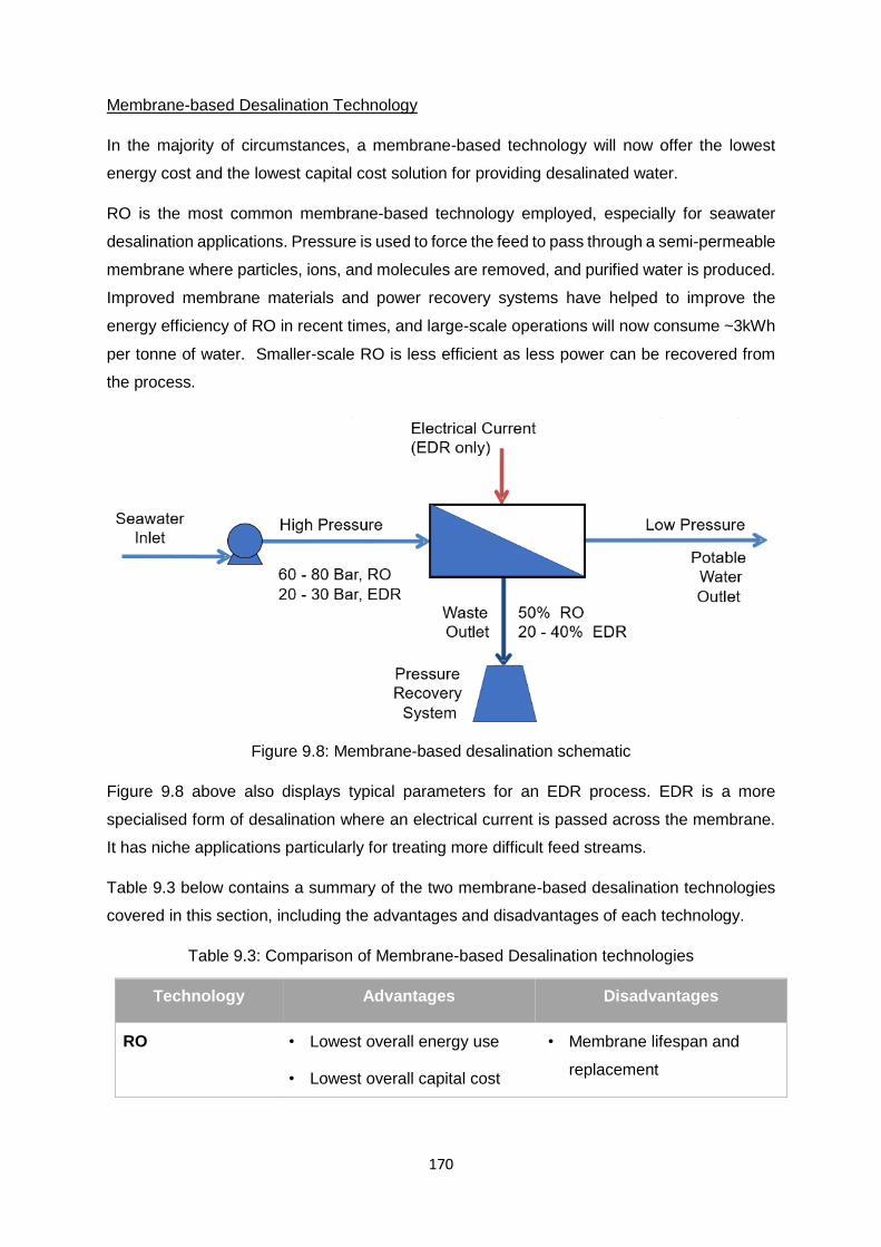
170
Membrane-based Desalination Technology
In the majority of circumstances, a membrane-based technology will now offer the lowest
energy cost and the lowest capital cost solution for providing desalinated water.
RO is the most common membrane-based technology employed, especially for seawater
desalination applications. Pressure is used to force the feed to pass through a semi-permeable
membrane where particles, ions, and molecules are removed, and purified water is produced.
Improved membrane materials and power recovery systems have helped to improve the
energy efficiency of RO in recent times, and large-scale operations will now consume ~3kWh
per tonne of water. Smaller-scale RO is less efficient as less power can be recovered from
the process.
Figure 9.8: Membrane-based desalination schematic
Figure 9.8 above also displays typical parameters for an EDR process. EDR is a more
specialised form of desalination where an electrical current is passed across the membrane.
It has niche applications particularly for treating more difficult feed streams.
Table 9.3 below contains a summary of the two membrane-based desalination technologies
covered in this section, including the advantages and disadvantages of each technology.
Table 9.3: Comparison of Membrane-based Desalination technologies
Technology Advantages Disadvantages
RO • Lowest overall energy use
• Lowest overall capital cost
• Membrane lifespan and
replacement

171
Uses high pressure
membrane to
exclude salts
• De-facto standard for new
desalination installations
worldwide
• Easily fouled – needs good
pre-treatment and equipment
care
• Cannot be cleaned using
chlorine-based biocides
• Uses power, not directly
LGH, to drive the process
EDR
Uses membrane and
electrical current to
exclude salts
• Less sensitive than RO to
silicates and particulates
• More robust – can use harsh
cleaning chemicals
• Can be used for specialist ion
recovery
• Higher capital and operating
costs than equivalent RO for
“routine” duties
Future Technology
There are a number of desalination technologies that have been developed in recent times
and have the potential to dramatically change the industry norms.
High Temperature Reverse Osmosis is one such technology that is commercially available
already and has demonstrated significant benefits compared to traditional technology. When
operated at 70°C the pressure drop across the unit is approximately only 30% of the pressure
drop when the unit is running at 25°C. If LGH can be used to increase the temperature of the
feed, it results in a direct saving in high value power.
Another promising technology as shown in Figure 9.9 below is Forward Osmosis.

172
Figure 9.9: Forward Osmosis desalination schematic
In a Forward Osmosis system it is the water, not the salts, which is absorbed into an Ammonia
/ Carbon Dioxide solution. LGH, at a very low temperature, can then be used to boil off the
solution leaving pure water as the product. This technology is now commercially viable, and a
number of pilot plants have been operating successfully, with claims of much lower specific
energy use when compared to traditional technology.
Desalination Summary
While desalination is one means of using waste LGH that is available, there are many
technologies that need to be considered. Based on energy efficiency, the preferable option is
to use LGH (if available in the range of 70°C to 150°C) to generate power, and then to use the
power to operate a RO desalination unit. For very low-grade waste heat (< 70°C) thermal
desalination is often the only practical use for the heat. In this situation MED is recommended
as it is generally the most efficient and best suited to low temperature heat sources.
In the future other technologies, such as Forward Osmosis, may become the technology of
choice for thermal desalination as they show promise for providing even more energy efficient
recovery of LGH.

173
9.5 Technology Selection
There is no standard definition or measurement for what is considered Low Grade Heat. In
some industries (for example smelting) there can be significant amounts of waste heat that
exist at temperatures exceeding 200°C. In other industries (for example food and beverage)
waste heat is regularly captured and utilised at temperatures of 50°C or less. The definition of
LGH is very industry dependent, but for the remaining sections of the chapter we will consider
waste heat below 150°C to be LGH. This is a typical value that is used in a number of energy
intensive industries such as refining and petrochemicals.
Below 150°C LGH can be further split in to smaller temperature ranges depending on the
quality of the heat, and therefore the potential uses for the waste heat:
Below 150°C it is typically not economically viable to recover LGH to generate LP
steam for the site header system,
Below 110°C it is typically not economically viable to recover LGH to generate LP
steam at atmospheric conditions,
Below 90°C it is typically not economically viable to recover LGH to drive an absorption
chiller,
Below 30°C LGH streams typically approach the temperature of the site cooling water
system.
The diagram in Figure 9.10 visually displays the nominal ranges of LGH that will be used in
the following sections.
Figure 9.10: Definition of Low Grade Heat
There are various options for recovering the energy from LGH – each option relies on different
technologies, and results in different outputs as shown in Figure 9.11. In order to reach the

174
best outcome for an individual site it is necessary to carefully evaluate the alternative LGH
recovery options based on a number of criteria:
Technical potential for LGH recovery at various temperature levels,
Economic value of useful output (heat, chilling, water),
Capital cost of the various recovery routes.
Figure 9.11: Energy inter-change
The alternative options will now be considered for each temperature range from Figure 9.11.
Waste Heat in the 110°C – 150°C range:
The most valuable use for LGH in the range of 110° to 150°C is process heating.
Implementation is easy and low cost as only simple heat exchangers are typically required.
However, the main limitation is the demand for LGH, otherwise known as the heat sink, as
explained in earlier chapters.
The possible uses for 1 MWh of waste heat are quantified and compared in Figure 9.12 below.
A number of economic assumptions have been made for the background calculations,
however the high-level comparison should be valid across a range of industry operating costs.

175
Figure 9.12: Comparing possible uses for 1 MWHth of heat in 150 oC to 110 oC Range
If process heating is not viable, the next best option for utilising the LGH is to generate power
using a condensing turbine as shown below in Figure 9.13.
Figure 9.13: LGH for Power Generation
There are three different ways in which the power can be utilised, and they all have similar
values:
To reduce site power import (or to export to the grid)
To produce desalinated water
To produce chilled water
The capital costs for implementing these projects will be high due to the multiple energy
conversions that are required. The economic viability will depend on the cost of power import.

176
Instead of using mechanical chilling to produce chilled water (via steam and power) from waste
heat, it is also possible to generate chilled water more directly using absorption chilling as
shown in Figure 9.14.
Figure 9.14: LGH for Chilled Water using Absorption Chilling
Given the same amount of waste heat, the performance of the two methods for generating
chilled water is quite similar:
The mechanical chilling system can produce 700 kW of chilling duty from 1 MW of
heat, whereas the absorption chilling system can produce 650 – 700 kW of chilling
duty,
The capital cost of absorption chillers is lower,
Absorption chillers are less flexible as power has many applications,
Typically, absorption chillers are preferred if a consistent demand for chilling duty
exists.
Waste Heat in the 90°C – 110°C range:
Once the temperature of the LGH drops below 110°C generating steam becomes much
more difficult or expensive, and below 100°C a vacuum is required. Saturated steam will
condense in turbines and therefore a certain level of superheating is required before steam
is provided to the header system.
The possible uses for 1 MWh of waste heat at 90°C – 110°C are quantified and compared in
Figure 9.15.
Figure 9.15: Value of 1 MWHth of heat at 90°C – 110°C

177
Once again, process heating is the best use of the LGH if a heat sink exists, and its value
remains unchanged at 0.48 MM US$/y. It may be possible to generate hot water as a heat
transfer medium if the heat supplier and the heat user are located a long distance from each
other.
Absorption chilling is still possible, however power can no longer be generated using
condensing turbines. Instead power would need to be generated using an Organic Rankine
Cycle with an efficiency of only 8 – 9%. If the site has a chilled water demand it is likely that
absorption chilling will be more economical than ORC due to the lower capital costs.
Thermal desalination remains the lowest value option.
Waste Heat in the 30°C – 90°C range:
Below 90°C it becomes much more difficult to economically utilise LGH. Absorption chilling is
no longer an option as the waste heat is not hot enough to boil the brine solution.
The possible uses for 1 MWh of waste heat at 30°C – 90°C are quantified and compared in
Figure 9.16 below.
Figure 9.16: Value of 1 MWHth of heat at < 90°C
Recovering the LGH for process heating is now significantly the best option, and still has the
same economic value. However, it is likely that the process heat sink will be much smaller
than the supply of waste heat.
At the higher end of the temperature range an ORC is still feasible for power generation. Using
LGH at 70°C the ORC will have an efficiency of around 4%, and the returns diminish rapidly
as the waste heat temperature drops further.
Thermal desalination is the only viable remaining option for LGH below 70°C.

178
9.6 Summary
There are numerous technologies that are available for recovering energy from LGH. All the
technologies mentioned here are commercially proven, and in a high energy cost location
such as Singapore, many of them may prove to be economical. Figure 9.17 below provides
a Preferred Technology Map for the technologies discussed in this chapter.
Figure 9.17: Preferred Technology Map
As every site is different, a detailed energy strategy is required to identify the optimal use of
LGH, taking in to account the heat supply and demand profiles as well as local economic
criteria. This strategy can often include simulation and modelling, pinch analysis (to maximise
the implementation of direct heat transfer) and TotalSite Pinch (to fit the LGH solution with the
site wide utility system). The next chapter will elaborate on these topics further and
demonstrate that significant benefits can be achieved.
9.7 References
Selected material included in this chapter has been sourced from KBC (A Yokogawa
Company).

179
9.8 Exercises
1. Discuss Low Grade Heat (LGH) recovery.
a) What temperature range can be considered LGH?
b) What are the most appropriate forms of recovery?
c) How is pinch analysis used to quantify the site demand for LGH and utilities?
d) Describe the main processes.
e) How do capital costs compare for the various recovery technologies?
f) How do operating costs/efficiencies compare?

180
Chapter 10
Site Wide Planning for Energy Improvement Strategies
By
Andrew Morrison
10.1 Overview
Many energy improvement opportunities are not entirely confined within the bounds of an
individual process unit. Instead, they rely on interactions and modifications across multiple
process units and the site utility system. A structured approach is required to ensure that
individual projects do not conflict, and to ensure that the best overall strategy is selected for
the site.
This chapter describes an approach for improving energy performance across an overall site,
or in fact multiple sites, in the following sections.
Section 10.1 Overview
Section 10.2 Site Source/Sink Profiles
Section 10.3 Analysing the Utility System
Section 10.4 Total Site Summary
Section 10.5 Total Area Analysis
Section 10.6 Total Site Analysis for Low Grade Heat Recovery
Section 10.7 Summary
Section 10.8 References
Section 10.9 Exercises
This chapter continues to build on some of the techniques introduced in Chapters 3 to 8,
including the use of Composite Curves and Grand Composite Curves. A basic understanding
of these principles is required and assumed prior to commencing this chapter.
The content in this chapter also links strongly to the concept of LGH recovery that was
introduced in Chapter 9, and the case study further demonstrates the importance of fully
understanding the impact that various potential projects could have on the site utility system.
The learning outcomes of this chapter on Site Wide Planning for Energy Improvement
Strategies are:
1. Understand the need for a long-term strategic plan to improve energy performance
across multiple process units

181
2. Describe a structured approach for modelling and analysing heat integration of a total
site including the utility system
3. Recognise that the concept can be further extended to multiple sites
10.2 Site Source/Sink Profiles
Most operating sites have some form of process utility requirement that is provided either by
an external party or by the site utility system. Common forms of utility include:
Fuel (for direct process heating in furnaces, or to generate steam in boilers)
Steam (for direct consumption or process heating)
Electricity
Cooling water
Figure 10.1 displays a simple schematic of a typical utility system. By analysing the diagram,
we can immediately obtain a high-level understanding on the site’s utility requirements:
The site has 3 processes that consume and generate utilities:
o Process A consumes LP steam and cooling water and generates both MP and
HP steam. Process A also includes a furnace that consumes fuel.
o Process B consumes HP steam, LP steam and cooling water.
o Process C consumes HP steam and MP steam, and generates LP steam.
Process C has no cooling water demand.
A multi-extraction steam turbine generates the HP and LP steam that is required by
the process units:
o There is no need to generate MP steam for Process C as it is currently
generated by Process A.
o The steam turbine also condenses a portion of the steam to generate more
power.
Power generated by the steam turbine can be consumed by the process units:
o The arrows suggest that power can also be imported or exported, depending
on the site’s power balance.
Fuel is consumed in the furnace in Process A and also in the boilers that generate the
steam for the multi-extraction steam turbine.

182
Figure 10.1: Utility system of a typical site
Figure 10.1 is a very simple representation and additional information can be displayed on the
same diagram to provide further details. This includes further information on the utility system
configuration (steam header let-downs, condensate recovery system, etc.), or quantitative
information (steam header pressures, flow rates, etc.).
If modifications are made to any one of the process units it will result in a new overall utility
demand profile for the site, which may not be possible to meet using the existing utility system.
There are different ways to meet the new individual process utilities demands. Investing in the
utilities systems may be more cost-effective in the short term, whereas investing in the process
heat recovery system may eventually result in greater savings when, for example, the
installation of a new boiler can be avoided.
The aim of a typical Total Site study is to provide a “roadmap”, or prioritised plan for multiple
projects, to lay out in what order potential site improvements should be made.
A long-term strategic plan or roadmap is required to:
Guide financial investments in energy efficiency of the existing processes and utility
system
Ensure compatibility of future initiatives (e.g. expansion or debottlenecking studies)
Take into account future events such as changes to environmental legislation, planned
shutdowns, etc.

183
Review all possible options and strategies instead of progressing in the direction of a
non-optimal outcome.
The basic approach for setting up a Total Site model is to begin by choosing the
thermodynamic representation for each process unit. Each process unit is categorised into
one of three different options:
‘Black’ Box – for process units that are small energy users and where no investment
is planned for modifying the unit.
‘Grey’ Box – for process units where the intention is only to investigate improvements
to the process/utility interface.
‘White’ Box – for process units where a full Pinch Analysis will be completed to find the
scope for heat recovery improvements within the process unit.
Careful consideration is required when deciding which processes will be “white-boxed” and
“grey-boxed”. There are no definitive rules, but the overall results can differ greatly if it is
assumed that individual process units can first be brought to a high level of efficiency before
improving the site-wide utility system. Experience and rational assumptions should guide the
engineer in the first instance.
Individual models will be generated for each process unit using a specific methodology
depending on how the process unit was categorised. The models are then combined to
produce Site Source/Sink cooling and heating profiles.
Black Box Processes
Units are treated as “Black Boxes” if it is decided that their internal configuration and operation
will not be optimised by implementing new energy recovery projects. Their existing utility
loads and levels (for example, pressure of steam demand) are kept constant for the Total
Site analysis.
Figure 10.2 displays Process A that has been categorised as a Black Box process. Process
A requires both 3-bar steam and cooling water, and both these requirements can be
represented on a Temperature – Enthalpy plot.

184
Figure 10.2: Black Box Processes
To model the fact that existing utilities must be used, the utility sinks and sources are specified
at temperatures that would allow this to happen. For instance, the heat sink above is defined
at the condensing temperature of 3-bar steam minus a suitable minimum ∆T, to force the
choice of that utility, regardless of the actual process temperatures that are achieved by
heating with that steam.
All process-to-process matches are excluded from the analysis.
Grey Box Processes
Units are treated as “grey boxes” if it is decided that changes will only be allowed in the choice
of utility for one or more of their existing duties. The existing utility loads are kept constant for
the Total Site analysis, but the levels (i.e. temperatures) of utilities can be optimised. This
could mean that an existing MP steam user is switched to a new IP steam level, if this is found
to be more economical from the analysis.
Figure 10.3 displays a process unit that has been categorised as a Grey Box process. Similar
to Process A, it currently has a demand for both 3 bar steam and cooling water, however this
time the requirements are represented differently on the Temperature – Enthalpy plot.

185
Figure 10.3: Grey Box Processes
The process stream data for the existing utility consumers are plotted at the actual process
temperatures. For example, one of the streams is process air that is being heated by steam
from 10°C to 80°C. These temperatures are used to produce the composite curve.
All process-to-process matches are still excluded from the analysis.
White Box Processes
“White box processes” are considered to have the potential for improving energy recovery
within the process unit, prior to investigating site wide energy improvement opportunities.
Therefore, they are first optimised using traditional pinch analysis techniques as covered in
the earlier chapters of this reference manual. This additional step minimises both the existing
loads and the levels of the utilities required by the process unit before adding their
contribution to the Total Site Analysis.
Figure 10.4 displays a process unit that has been categorised as a White Box process. The
Composite Curves have been generated for the process unit, as has the Grand Composite
Curve. The Heat Sink and Heat Source portions of the Grand Composite Curve are then
extracted from the Temperature – Enthalpy plot.

186
Figure 10.4: White Box Processes
This approach makes the assumption that heat recovery optimisation is implemented to
achieve the pinch analysis targets before any utility system improvement is carried out.
Therefore, only the ideal utility demands from White Box processes are included in the overall
Total Site analysis.
Total Site Profiles
The individual white, grey and black box utility demands are combined to construct the ideal
Site Source/Sink curves as shown in Figure 10.5.

187
Figure 10.5: Total Site Profiles
The Site Heat Source Profile is created from the compilation of three separate streams:
The Heat Source from the Black Box Process (fixed utility data)
The Overheads stream from the Grey Box Process, and
The Heat Source portion of the GCC from the White Box Process
Likewise, the Site Heat Sink Profile is compiled from three streams:
The Heat Sink from the Black Box Process (fixed utility data)
The Process Air stream from the Grey Box Process, and
The Heat Sink portion of the GCC from the White Box Process.
In the example above there is only 1 Black Box process, 1 Grey Box process and 1 White Box
process included; however, on many sites, there will be several of each type of process.
Obviously, additional process units increase the complexity of the Total Site model as the
various individual composite curves begin to overlap. While this process can be carried out
manually, it is more common to employ specialised software to carry out Total Site analysis.
The Site Source / Sink curves are both plotted so they just touch the vertical axis of the chart.
Because the curves are not allowed to overlap, there is no implied integration between the
individual process units. All heat transfer is therefore via the site utility systems; hence the
autonomy of the individual processes is recognised.

188
10.3 Analysing the Utility System
The Site Source / Sink Curves are a very useful tool for analysing the overall site utility system
and understanding where opportunities from heat recovery projects may exist.
It is usually possible to create (a lot of) LP steam from process waste heat. However, this low-
level steam will only end up being vented if there are no heat sinks where the energy can be
utilised elsewhere on the site. The Site Source / Sink curves identify the ideal quantities of
steam to be generated at specific temperature levels. Beyond these quantities there is no
value in generating steam and it makes economic sense to cool the process against cooling
water and not against more expensive boiler feed water.
Figure 10.6: Analysing the Utility System using Source / Sink curves
Figure 10.6 displays the Site Source / Sink Curves from an example site. The Site Source
Curve is displayed on the left and below the curve the ideal steam generation targets have
been included, while the Site Sink Curve is displayed on the right and above the curve the
ideal steam consumption targets are shown.

189
The enthalpy scale on the horizontal axis can be utilised to calculate the steam generation or
consumption targets at any given temperature level. Ideally, the Source / Sink curves and their
respective targets are as close together as possible.
A Real Life Example
As mentioned previously, the first step is to identify the key process units and to define the
Black Box, Grey Box and White Box processes. It is common for over 70% of potential savings
to come from just 30% of the process units. Table 10.1 provides a typical breakdown of the
scope for energy reductions from a selection of process units.
Table 10.1: Energy Use of individual Process Units
Some process units will have a large savings potential from energy recovery projects that can
be implemented entirely within the bounds of the individual unit. Other process units can be
“black-boxed” immediately as it is clear that there is no value in exploring improvement
opportunities. Thus, some units will be marked for improvement, whilst others will be kept
running at existing conditions for as long as possible. There is some judgement in deciding
how to represent the individual process units, and if time permits it may even be necessary to
create the Site Source / Sink profiles under multiple assumptions to arrive at a conclusion.
Figure 10.7 displays a schematic of the existing utility system from the example site. There
are four steam headers (HP, MP, IP and LP) and the various flow rates have been shown.

190
Figure 10.7: Existing Site – Utility System
In this example, the existing steam turbo generator is the key bottleneck for the utility system.
There is a 60 t/h surplus of LP steam, which mainly arises as pass-out from the driver turbines.
Of the total surplus LP steam only 40 t/h can be passed out through the condensing stage of
the turbo generator. Therefore, 20 t/h of LP steam must be vented.
The Site Source / Sink Profiles for the existing example site are displayed in Figure 10.8.
Boiler

191
Figure 10.8: Existing Site – Site Source / Sink Profiles
The first thing that is evident is that there are “gaps” between the Existing Steam Generation
Profile and the steam generation targets curve. This indicates that compared to the existing
operation, additional steam can be generated at higher temperature levels. There are also
“gaps” between the Existing Steam Consumption Profile and the steam consumption targets
curve. Again, this indicates that improvements are possible. In this case it implies that it should
be possible to consume more steam at lower temperature levels.
The utility system schematic identified that the steam turbo generator was the key bottleneck.
The steam consumption targets show that much more steam can be consumed at the LP level,
with reduced demand for MP and HP steam. These changes would result in the turbo
generator passing out LP steam instead of taking it in.

192
Figure 10.9: Improved Site – Site Source / Sink Profiles
Figure 10.9 displays the Site Source / Sink Profiles for the example site if improvements were
made to the individual process units. There are two general rules that should be followed:
Maximise steam generation pressures
Minimise steam consumption pressures
The impact of the steam generation and consumption targets can be simulated and checked
using the site utility system model. Figure 10.10 displays a schematic of the utility system for
the improved example site.

193
Figure 10.10: Improved Site – Utility System
The changes to the steam targets that would result from improving the individual process units
have a significant effect on the site utility system:
More steam is consumed at the LP and IP levels, and less steam is consumed at the
MP level.
The LP vent is eliminated and there is now a pass-out flow from the steam turbo
generator.
A new steam turbo generator produces additional power to help reduce the overall site
import.
More HP steam is generated in the process units and the HP steam demand from the
site boilers is significantly reduced.
Table 10.2 summarises the changes in process steam consumption and generation for this
example.
Boiler

194
Table 10.2: Comparison of Existing and Improved scenarios
The last column in the table shows the saving in net steam demand from the site utility system
– a negative value implies an increase in steam demand. The significant shift from HP and
MP steam demand to IP and LP steam demand is quite typical. The steam saving at the HP
level is the major factor in reducing the total costs.
While every site is different, a number of the improvement opportunities that were identified
during this example project are commonly found:
1. New process heat exchangers to recover additional heat and therefore reduce utility
consumption.
2. Optimised distillation column feed conditions to reduce reboiler load.
3. Maximum use of steam at the cheapest pressure levels.
4. Heat recovery to preheat deaerator feed water to reduce deaeration steam.
5. Optimised operation of the utility system.
It is interesting to consider how each of these general opportunities are identified. The
improvement opportunities listed in items 1 and 2 will only be identified in process units that
are categorised as White Box processes. Altering the levels of steam use will be found for
process units that are categorised as Grey Box processes. Changes to the utility system
operation will normally be derived from an analysis of the separate steam system model.
The utility system model is an important tool when carrying out an energy improvement project
across the overall site. Practical and feasible steam savings are dependent on the site steam
balance and must account for factors such as driver demands / exhausts, steam vents and
system operating constraints. The model also allows realistic co-generation options to be
evaluated and the savings from individual (or combinations of) projects to be verified. The
steam savings can be accurately converted to fuel and power changes for the actual site

195
operating conditions and constraints, thus avoiding the use of inaccurate (or incorrect)
marginal steam costs.
The overall results from the example improvement study showed large energy savings while
simultaneously providing improvements in operating flexibility:
Boiler steam generation and utility operating costs were both reduced by 35%.
Electricity produced by cogeneration increased by 7%.
The steam turbo generator was debottlenecked and the LP steam vent was eliminated.
1 site boiler could be shutdown.
10.4 Total Site Summary
The proposed approach for Total Site energy improvement projects is summarised in the
diagram in Figure 10.11.
Figure 10.11: Total Site Summary
Initially in Phase 1, a larger number of the process units may be categorised as White Box or
Grey Box processes. After the preliminary analyses, a decision may be made that some
should be downgraded to Grey Box or Black Box processes instead. This reduces the number
of process units where a detailed pinch analysis study is required, which in turn reduces the
duration of the overall study.

196
Projects within individual process units that are identified as part of the White Box analysis
can be developed in parallel with the definition of the utility systems projects. They are then
combined in the site roadmap, an example of which is provided in Figure 10.12.
Figure 10.12: Example roadmap
The full derivation of the roadmap is a manual procedure typically based on multiple software
runs and will not be explained in depth in this manual.
There are many benefits of the structured Total Site methodology as explained in this chapter.
The systematic approach ensures that all opportunities are identified and it allows various
alternatives to be compared at a high level without the need to complete a full detailed
analysis. The optimum configuration can be selected and verified using the site utility system
model.
10.5 Total Area Analysis
The Total Site techniques explained in sections 10.2 – 10.4 can also be utilised to analyse
opportunities for heat sharing between companies. Known as Total Area Analysis, these
studies were first performed at Rotterdam in the Netherlands. Over 80 participating companies
were involved in the study and >1,000 MW of heat was found to be available at temperatures

197
exceeding 100°C. The study estimated that 15 – 25% of the available heat recovery
opportunities would be implementable.
Total Area Analysis is typically carried out in 2 phases:
Phase 1: Study of energy supply and demand
o Total Site analysis is carried out for each individual company, and the energy
patterns (e.g. seasonal or daily variations) are investigated.
o The analysis is extended to include clusters of companies.
o The overall Total Area Analysis is carried out including all companies.
Phase 2: Identification and definition of project opportunities
o Detailed project development of opportunities identified within individual sites.
o Detailed project development of selected key opportunities that span multiple
companies to define the heat sharing economics.
o Capital cost estimating and detailed engineering.
10.6 Total Site Analysis for Low Grade Heat Recovery
In Chapter 9 Low Grade Heat Recovery was introduced, and a priority for utilising available
waste heat sources was established:
1. Process Heat Recovery
2. Generate Steam (if temperature permits)
3. Absorption Chilling
4. Organic Rankine Cycle
5. Thermal Desalination
We can now use the Site Source / Sink Profiles to evaluate the potential for each type of LGH
recovery. Figure 10.13 displays Site Source / Sink curves for an example petrochemical
complex that will be used to explain this concept.

198
Figure 10.13: Site Composites – Petrochemical Complex
The Site Heat Source curve is displayed on the left, and both the Target Cold Utility and
Existing Cold Utility have been plotted below. On the right is the Site Heat Sink curve, with the
Target Hot Utility and Existing Hot Utility also plotted.
By evaluating the gaps between the “Target” and “Existing” plots, initial conclusions can be
drawn, such as:
There is an existing demand for chilled water (below ambient conditions), some of
which might be possible to switch to cooling water.
There is potential to generate steam at higher levels.
There is potential to consume steam at lower levels.
However, even if all of the opportunities above are optimised there will still be a significant
amount of waste heat (>500 Gcal/h currently matched with cooling water) that cannot be
utilised elsewhere in the site. To further improve the overall energy efficiency possible, new
utilities can be explored.

199
Figure 10.14: Define possible new utilities
Figure 10.14 highlights three new utilities that could be considered in this example:
Very Very Low Pressure (VVLP) steam could be generated at a pressure of
approximately 0.5 bar. This steam could then be utilised to drive an absorption chiller
or a steam turbine.
Hot Water at a temperature high enough to drive an absorption chiller.
Hot Water for process heating.
Figure 10.15 displays the Site Source / Sink Profiles after the new utilities have been included.
A portion of the VVLP steam and Hot Water can be supplied to the Site Heat Sink.
Hot Water
VVLP Steam
Hot Water for
chilling

200
Figure 10.15: Site Composites after new utilities addition
It is observed in this example, and in fact in most cases, that the potential for low temperature
utility generation far exceeds the process heat demand.
Table 10.3 summarises the new utilities that were proposed for this petrochemical complex.
Table 10.3: New utilities proposed for complex
New Utilities Generation
(Gcal/h) Process Use
(Gcal/h) Surplus (Gcal/h)
Comments
VVLP Steam 67.4 2.6 64.8 Surplus available for steam
turbine or to drive chiller
Hot Water (> 90oC)
28.9 3.9 25.0 Surplus available for chilled water generation
Low Grade Hot Water (70 - 90oC)
76.2 19.0 57.2 Surplus available to drive ORC
The overall savings for the petrochemical complex identified in this example are as follows:
10 MM US$/y in reduced process heat demand,

201
5 MM US$/y in VVLP steam turbine power generation, and
2 MM US$/y in reduced refrigeration system power requirements.
This example demonstrates that an overall utility model is not just a valuable tool for day-to-
day operations of the site, but it is also a valuable tool for engineering planning. Carrying out
a “big picture” analysis by combining Pinch Analysis, Utility Optimisation and an understanding
of the present and future constraints of the site avoids a situation where sub-optimal
technologies or solutions are pursued too early in the study. For example, it does not make
sense to build a new cogeneration plant based on today’s steam demands before assessing
how much steam can be saved across the site. Likewise, smaller heat recovery projects
should be reviewed in the site-wide context to ensure they are the best option based on overall
hot and cold utility demands.
Heat sharing or utility integration with neighbours should also be considered. The
petrochemical case study from above is expanded to now consider multiple complexes.
Figure 10.16 provides an overview of the total area.
Figure 10.16: Total Site Analysis of Multiple Complexes

202
The total area is made up of 3 separate complexes that share a common utilities system.
Each complex has utility demands that are met by the common system. By looking closer at
two of the complexes it is possible to identify opportunities for further energy savings:
The Site Source / Sink curves for Complex 1 are shown in the top right of Figure 10.16.
o There is potential to generate VLP steam and Hot Water.
o There is limited potential for using these generated utilities within the Complex.
The Site Source / Sink curves for Complex 2 are shown in the bottom right of Figure
10.16.
o There is a large demand for low temperature utilities.
o There are insufficient heat sources available within the Complex.
Recovering heat from one complex to another has the potential to save a large amount of heat
worth approximately US$17 MM/y. The heat recovery project would also reduce the size of
the required cooling water system.
In the example of the three Complexes there were also further Low Grade Heat recovery
opportunities identified:
Additional process to process recovery via a Hot Water Loop
Additional VLP Steam recovery to generate 22 MW of power
Complex 2 was designed to include a heat pump.
o This was a rational design in isolation as Complex 2 has a heat deficit and can
use the heat pump to recover energy from a condenser.
o However, in a total area integrated design utilising hot water from other units
saves the capital costs of a new compressor as well as the operating costs of
power to drive the heat pump compressor.
Additional heat recovery to utilities by preheating feed water to the deaerator.
Likewise, other opportunities to increase the efficiency of the common utility system were
identified as part of the study.
Replacing planned furnaces with steam heaters increased the cogeneration heat
demand, which improved the overall cycle efficiency by approximately 5%.
Reduced steam header pressures also improved the overall utility system efficiency.

203
The overall benefits identified in this example study were calculated to be a reduction in
required capital costs of over USD100 MM and a reduction in operating costs of approximately
USD200 MM/y.
10.7 Summary
There are numerous ways to improve energy efficiency in an operating site and a strategic
plan is required to consider all the various options and to ensure that the optimum strategy for
the overall site is identified and implemented. Typically, this strategy will include multiple
individual opportunities that interact directly or via the site utility system.
A methodology introduced in this chapter is one such approach for considering the total site.
The example case study demonstrated that following the methodology and utilising a utility
system model to verify project savings can result in significant improvements and economic
benefits.
The same Total Site approach can be extended to multiple sites using Total Area Analysis.
10.8 References
Selected material included in this chapter has been sourced from KBC (A Yokogawa
Company).

204
10.9 Exercises
1. Consider the diagram of a utility system shown below, with particular focus on the
aspects highlighted in yellow.
Pinch analysis identifies 1 process pinch at a temperature between IP and MP steam. It also
identifies 4 utility pinches:
HP – MP
MP – IP
IP – LP
LP – Cooling Water
There is cross-pinch heat transfer occurring at each of these pinch temperatures. How
significant is the economic impact of the cross-pinch heat transfer?

205
A) Process Pinch
A. Very significant
B. Not significant
C. Not enough information to calculate
B) Pinch: HP - MP
A. Very significant
B. Not significant
C. Not enough information to calculate
C) Pinch: MP - IP
A. Very significant
B. Not significant
C. Not enough information to calculate
D) Pinch: IP - LP
A. Very significant
B. Not significant
C. Not enough information to calculate
E) Pinch: LP – Cooling Water
A. Very significant
B. Not significant
C. Not enough information to calculate
HINT: Think about what happens if demand decreases above the pinch and demand
increases below the pinch. For example, the process previously required 1 t/h of HP steam
but now it uses 1 t/h of MP steam. Will this change reduce costs?

206
2. Consider the diagram below.
The diagram shows a Site Source Sink Profile (SSSP) that was generated during a Total Site
pinch analysis.
Briefly explain how the SSSP is generated.
What opportunities for improvement exist?
What do each of the circles highlight?

207
Chapter 11
Other Energy Recovery Techniques and Technologies
By
Andrew Morrison
11.1 Overview
Pinch Analysis often recommends that new heat exchangers are installed or that the area of
existing exchangers is increased to allow additional heat recovery. Implementing these
modifications can often be challenging due to factors such as space constraints, economic
feasibilities or available downtime. Advanced exchanger technologies can help to overcome
these challenges.
There are many items of equipment commonly found in industry that have an impact on the
amount of energy consumed by the process. A basic understanding of how these equipment
items work, as well as the factors that impact energy efficiency of the equipment, is valuable
when carrying out an energy improvement study.
This chapter provides an introduction to Energy Recovery Techniques and Technologies in
the following sections:
Section 11.1 Overview
Section 11.2 Heat Exchangers
Section 11.3 Power Recovery
Section 11.4 Heat Pumps
Section 11.5 Rotating Equipment Efficiency
Section 11.6 Summary
Section 11.7 References
Section 11.8 Exercises
This chapter is designed to provide a general awareness of each of the topics listed above.
Readers should have no problems locating more detailed information online for topics relevant
to their specific situation.
Learning outcomes of this chapter on Energy Recovery Techniques and Technologies are:
1. Gain an understanding of the technologies available to put pinch opportunities into
practice:
a. Heat Exchanger Enhancements

208
b. Advanced Exchanger Technologies
2. Gain an understanding of other energy recovery techniques and technologies:
a. Power Recovery
i. From Liquids
ii. From Gasses
b. Heat Pumps
c. Rotating Equipment Efficiency
11.2 Heat Exchangers
Heat exchangers were introduced in Chapter 2 of this manual and a range of different heat
exchanger (HE) types and configurations were discussed.
A shell-and-tube HE is still the most conventional type found throughout the process
industries. When pinch analysis recommends increasing the area of an existing shell-and-tube
HE, the most basic way to add heat transfer area is through the introduction of a new shell.
However, this may not be practically viable due to factors such as space constraints.
Therefore, another option is to enhance the heat transfer coefficient of the existing HE as
discussed in section 2.6 of this manual.
Heat transfer enhancements can be classified as either shellside (baffles, finned tubes) or
tubeside (tube inserts, twisted tubes) and improve the heat transfer performance of existing
HEs without requiring additional space and at a reduced cost compared to replacing existing
HEs.
For each of the enhancements there can be various options and configurations to further
consider. As an example, commonly utilised baffles include:
Segmented baffles
Rod baffles
Expanded metal baffles
Helical baffles
There are also many other types of baffles, and each individual design provides a different
flow pattern within the HE that should be considered during the selection process.
Another option for increasing HE area while minimising space requirements is to utilise
compact heat exchangers. The most common example is the simple plate exchanger as
introduced in Chapter 2 and various multi-pass arrangements can be employed. There are
also many different types of plate exchangers:

209
Gasketed plate heat exchangers
Brazed plate heat exchangers
Welded plate heat exchangers
Various vendor-specific compact heat exchangers, such as Compabloc, Packinox and
Ziepack, are also available on the market, and readers are encouraged to investigate the
available options based on their process stream characteristics.
Chapter 2 briefly introduced pipe heat exchangers and furnaces, but in reality, many other
types of HE also exist. These range from large rotary HEs that are utilised in the process
industries for heating air from furnace stack gasses, through to tiny printed-circuit HEs with
stacked etched plates and diffusion bonding in the electronics industry.
11.3 Power Recovery
Power can be recovered from the pressure drop as a high pressure stream is reduced in
pressure to a low pressure stream. Power recovery extracts internal energy and cools the fluid
and a greater amount of energy recovery is possible from gasses when compared to liquids.
If a high-pressure stream reduces in pressure across a valve, as shown in the left of Figure
11.1 below, the result is isenthalpic in that the enthalpy of the stream does not change. Liquid
streams will incur a small temperature drop while gas streams will experience cooling as work
is carried out to expand the gas.
Figure 11.1: Power recovery from pressure drop
The diagram in the right of Figure 11.1 above displays an alternative scenario where the high-
pressure stream reduces in pressure across a Power Recovery Device. In this situation shaft
work (more commonly referred to simply as work) is extracted and the enthalpy of the stream
is reduced. Liquid streams will still experience a relatively small temperature drop while gas
streams will experience significant cooling as both work is carried out to expand the gas and
additional energy is extracted.

210
Hydraulic Pressure Recovery Turbines
To recover power from liquids an equipment item called a hydraulic pressure recovery turbine
(HPRT) is used. An HPRT can be thought of as a backward running pump:
A pump consumes work (power) to convert the low pressure inlet fluid to a high
pressure outlet fluid
An HPRT generates work (power) as a high pressure inlet fluid is converted to a low
pressure outlet fluid
Various reciprocating and centrifugal designs can be employed to improve efficiency based
on the process streams.
Common applications for HPRTs include, but are not limited to:
High pressure membrane reject streams
High pressure reactor outlet streams
Rich solvent streams in absorber or stripper systems
There are some reliability challenges that should be investigated when considering HPRTs.
Light components dissolved in the fluid tend to vaporise as the pressure of the stream drops.
The resulting bubbles can cause vibration and reduce the reliability of the equipment. To avoid
this issue, consider reducing the amount of pressure drop or cooling the process stream before
the HPRT. It should be noted that both of these options will result in reduced power recovery
efficiency.
Expanders
To recover power from gasses an equipment item called an expander is used. An expander
works in the same way as a steam turbine but utilises a different fluid. The high pressure gas
enters the expander where work is extracted, and a lower pressure gas exits at the outlet.
Common applications for expanders include, but are not limited to:
Gas turbines and steam turbines
Cryogenic systems such as those found in ethylene cracking
Specific processes such as PTA

211
Again, there are some reliability challenges that should be investigated when considering
expanders. Heavy components within the process stream may condense as the temperature
reduces. This can cause erosion, vibration and sometimes corrosion, all of which reduce the
reliability of the equipment. To avoid these issues, consider preheating or inter-stage heating,
which has the added benefit of increasing the overall efficiency of the expander.
Two Phase Expanders
Two phase expanders were developed in the mid-2000’s to overcome some of the issues with
expanding potentially multi-phase process streams. The equipment has a turbine type
geometry at the top, with a pump impeller type geometry at the bottom.
Common applications for two phase expanders include LNG liquefaction. As extra energy is
extracted as power the LNG is cooled further, hence the two phase expander can assist in
increasing production at the same time.
Generally, two phase expanders are reasonably reliable as they can handle both liquid and
vapour streams. However, it is important that the vapour fraction remains close to the design
conditions.
Once the shaft work is extracted, whether it be from an HPRT, expander or two phase
expanders, it must be exploited to provide value. There are typically two ways this can be
carried out.
The first option is to generate electrical power that is transferred to the site electrical grid. This
is the best option from a reliability point-of-view as if the power recovery device trips the
shortfall of electrical energy can be made up with increased power import. However,
traditionally this option was not popular in the process industries as there was a high cost
associated with frequency synchronizing equipment to send energy from small generators
back into the site grid. In the last 10 – 15 years the costs have dramatically reduced, and this
is now the preferred option in most scenarios.
The second option is to directly couple the power recovery device with a pump or compressor.
The pump or compressor power requirement can be topped up using a motor when required.
Reliability issues related to power trips need to be addressed through the installation of spare
equipment (for example, multiple pumps) leading to additional costs.

212
11.4 Heat Pumps
A heat pump, also known as a heat engine, works like a refrigeration system.
In a refrigeration system power is required to drive the compressor that converts a low-
pressure gas to a high-pressure gas. The high-pressure gas releases heat as it is condensed
in the condenser, and then a control device reduces the pressure of the liquid further resulting
in a low-pressure liquid / gas stream. This stream passes through the cooler where it absorbs
heat (providing the refrigeration) and is converted to a low-pressure gas to complete the cycle.
So high value power has been used to drive cooling at a lower temperature.
Figure 11.2 provides an overview of a heat pump.
Figure 11.2: Heat pump overview
The heat pump uses high value power (W) to upgrade an amount of heat (Q) from a lower
temperature source to a higher temperature sink. The total amount of heat transferred to the
heat sink is equivalent to (Q + W).
A decision must be made as to how a heat pump should be integrated into a process,
specifically with respect to the pinch point.
One option is above the pinch as shown in Figure 11.3.

213
Figure 11.3: Heat pump integration above the pinch
In Figure 11.3, Q units of heat from the process above the pinch are upgraded using power to
(Q + W) units of heat, also above the pinch. As a result, the hot utility consumption of the
process is reduced by W units, whilst the power consumption is increased by W units. In
effect, the power consumption has been increased to reduce the heat demand by the same
amount, which is usually not economical as power prices are higher on an energy basis.
Another option for integrating the heat pump into the process is below the pinch as shown in
Figure 11.4.
Figure 11.4: Heat pump integration below the pinch

214
In Figure 11.4, W units of power are being added to what was already a heat source. This
additional expensive electricity will eventually be rejected to cooling utility, which will most
certainly not be an economically attractive outcome.
In summary, integrating heat pumps entirely above or below the pinch is not appropriate.
Instead heat pumps should be integrated across the pinch point as shown in Figure 11.5.
Figure 11.5: Heat pump integration across the pinch
If the heat pump is integrated across the pinch it simultaneously reduces the hot utility
consumption by (Q+W) units and reduces the cold utility consumption by (Q) units. As a golden
rule, the appropriate placement of a heat pump is therefore always across the pinch.
The readers may note that integrating a heat pump across the pinch can be considered an
example of the Plus-Minus Principle that was introduced in Section 3.7 of this manual. The
total duty of hot streams above the pinch is increased, which leads to a reduction in hot utility
required by the process. At the same time, the total duty of cold streams below the pinch in
decreased, which leads to a reduction in cold utility required by the process.
To target the thermal design, it is possible to use the Grand Composite Curve (GCC) and treat
the heat pump as if it is two utility streams. This is shown in Figure 11.6.

215
Figure 11.6: Heat pump placement using the GCC
With the GCC, determining the levels for heat pump placement is relatively straightforward.
The cold part of the heat pump is equivalent to a cold utility, whilst the hot part of the heat
pump is equivalent to a hot utility.
The calculation of the duty can be a bit more difficult. In the example shown in Figure 11.6,
the duty on the hot side (Q2) is known. By enthalpy balance, Q1 = (Q2 – W). However, W is a
function of the temperature at the cold side, which is also unknown. Therefore, the cold side
temperature needs to be determined by iteration.
Similarly, if the cold side of the heat pump is limiting, the temperature at the hot side must be
determined by iteration. In Figure 11.6 the hot side of heat pump is limiting as Q2 touches the
GCC.
Note that as well as operating across a process pinch point, a heat pump can also operate
across a utility pinch as shown in Figure 11.7.
Figure 11.7: Heat pump placement across a utility pinch

216
In this example MP steam is reduced at the expense of additional LP steam.
Heat Pump Coefficient of Performance
As power is an expensive utility, the aim should be to minimise the work input to a heat pump,
and in practical applications the amount of power required will determine whether the heat
pump is economically viable.
The heat pump coefficient of performance (COP) can be calculated as a ratio of the useful
heat provided for each unit of work required.
COP = Q+W
W= 𝑓(T)
A higher COP results in lower operating costs for the heat pump. As shown by the COP
formula above, the COP is also a function of the temperature difference between the cold side
and the hot side of the heat pump.
Figure 11.8 displays two heat pumps that transfer the same amount of heat across the pinch
but with different COPs.
Figure 11.8: Heat pump COP
The heat pump on the right has a much higher COP and the operating costs compared to the
heat pump on the left would be significantly lower. In all cases, the aim should be to use heat
pumps across small temperature differences.
It should be noted that when a heat pump is installed the driving forces in the process are
reduced. Generally, this results in an increase in the capital cost of the heat exchanger

217
network. Heat pumps should generally be considered when both of the following conditions
apply:
The GCC displays a sharp “nose” at the pinch point
The operating temperature of the heat pump is below ~150°C
It is possible to make the GCC “nose” sharper by adjusting the process conditions and altering
the conditions of the process streams.
Common applications for heat pumps in process industries include Propane / Propylene
splitters and dryer vapour compression.
11.5 Rotating Equipment Efficiency
This section provides an overview of the efficient operation of rotating equipment commonly
found in the process industries. Reliability aspects are also briefly mentioned, but for more
detailed information readers should carry out further investigations and consult the equipment
providers.
There are two main categories of rotating equipment:
Energy Extractors
o Turbines (gas or steam)
Energy Users
o Compressors
o Pumps
o Fans and Blowers
Compressors increase the pressure of compressible gas, while pumps move fluid streams
and fans and blowers move gaseous streams.
Steam Turbines
The energy efficient operation of steam turbines depends on several parameters.
A small deviation in condenser vacuum from the optimum can produce a significant change in
power output. There are a number of reasons why the condenser vacuum may be poor:

218
The cooling water inlet temperature is high. This can be caused by high ambient
temperatures or humidity.
The cooling water flow rate to the condenser is insufficient.
The condenser tubes are fouled, damaged or some are blocked. Cleaning the
condenser can often help to overcome this problem
Air leaks into the condenser are occurring.
If the steam temperature and pressure at the turbine inlet are reduced, the turbine will produce
less power.
This parameter affects both condensing and backpressure turbines.
“Slow-rolling" is a commonly used technique where steam is constantly passed through the
turbine even when it is not generating power. It is used to keep turbines in hot stand-by
condition in case they are required to start-up quickly.
Slow rolling can consume up to 15% of the turbine’s nominal steam rate.
This practice is typically unnecessary with modern design turbines as they can start-
up from cold stand-by without any issues.
The use of hand valves, also known as overload valves, should be optimised especially when
the turbine is operating at part load.
Pumps
Pumping systems account for nearly 20% of the world’s electrical energy demand and range
from 25 - 50% of the energy usage in certain process industry operations.
Pump performance parameters change with its rotating speed following so called “Affinity
Laws”.
Flowrate is proportional to rotating speed
Head is proportional to the square of rotating speed
Power is proportional to the cube of rotating speed
Therefore, doubling the rotating speed of a pump increases power consumption by 8 times.
Conversely, a reduction in the rotating speed will greatly assist in reducing power
consumption. Flow control by speed regulation is always more efficient than using a control
valve because valves reduce flow, but not the amount of energy consumed.

219
There are several parameters that should be considered to ensure energy efficient operation
of pumps.
It is important to begin by selecting the right pump for the process conditions.
Pump efficiency peaks at a certain operating point, and the pump operation is less
efficient either side of these conditions.
However, given the design margin (and sometimes additional margins), pumps are
often oversized and tend to operate at a sub-optimal point.
Installation of VSDs, two-speed drives, lower rpm motors or smaller / trimmed impellers
can all help to improve the efficiency.
It is possible to control the flow rate of the pump by speed variation. A commonly used device
for reducing pump speed is a Variable Speed Drive (VSD) with continuous speed adjustments.
Mechanical VSDs have hydraulic clutches, fluid couplings, and adjustable belts and
pulleys.
Electrical VSDs are designed with eddy current clutches, wound-rotor motor
controllers, and variable frequency drives (VFDs).
o VFDs are the most popular option and adjust the electrical frequency of the
power supplied to a motor to change the motor’s rotational speed.
o VFDs have improved markedly in cost and reliability in recent years.
The major advantages of VSDs include:
o Improved process control, as VSDs can correct small variations in flow faster
that other methods.
o Improved system reliability, because the wear on pumps, bearings and seals
are reduced.
o Reduction of both capital and maintenance costs because control valves, by-
pass lines, and conventional starters are no longer needed.
o Soft starter capability, as VSDs allow the motor to have a lower startup current.
Another option is to install multiple pumps in parallel to meet the varying overall demand of
the process.
As an example, operating two pumps in parallel and turning one off when the demand
is lower, can save energy.

220
Pumps providing different flow rates can be used – it is not necessary for all pumps to
be the same size.
Elimination of by-pass control will improve the efficiency of the overall system.
Flow is sometimes controlled by recycling part of the pump discharge back to the pump
suction. This is clearly a waste of energy as the same fluid is pumped multiple times.
When a pump is oversized for the expected operating conditions a low capital cost option to
improve energy efficiency is to consider impeller trimming.
Changing the impeller diameter alters the impeller’s peripheral velocity.
Similar to the pump affinity laws, the performance of the pump is proportional to
impeller diameter:
o Flowrate is proportional to the cube of the impeller diameter
o Head is proportional to the square of the impeller diameter
o Power is proportional to the fifth power of the impeller diameter
It should be noted that the impeller should not be trimmed below 75% of its original
size, otherwise there is a risk of vibration due to cavitation.
Finally, a simple and reasonably energy-efficient way to reduce the flow rate is by starting and
stopping the pump, provided that this does not happen too frequently. An example where this
option can be applied is when a pump is used to fill a storage tank from which the fluid flows
to the process at a steady rate. In this system, controllers are installed at the minimum and
maximum levels inside the tank to start and stop the pump. Some companies use this method
to reduce peak power demand by only pumping during no-peak hours.
Compressors
There are two main types of compressors:
Positive displacement
Dynamic
In positive displacement compressors energy is added periodically to increase gas pressure,
and thereby reduce the volume of the stream. Positive displacement compressors generally
only handle lower flowrates, but they are able to achieve higher pressure ratios compared to
dynamic compressors. Common examples of positive displacement compressors include
reciprocating compressors and rotary screw compressors.

221
In dynamic compressors energy is added continuously to increase the gas velocities within
the compressor. Dynamic compressors use multi-staging to achieve higher compression
ratios. Common examples of dynamic compressors include centrifugal compressors and axial
compressors.
Compressor efficiency depends on the level of intercooling that takes place within the
compressor system. Compression can be:
Adiabatic (isentropic) if there is no intercooling
Isothermal if sufficient cooling is carried out such that the temperature of the fluid is
the same at the inlet and the discharge.
As isothermal compression requires less work input, most compressors involve some
intercooling but do not achieve the full isothermal ideal.
There are several parameters that should be considered to ensure energy efficient operation
of compressors.
The compressor inlet temperature should be minimised to reduce compression power.
Compressors consumes less power if the intake gas is colder. If the inlet temperature
increases from 15°C to 21°C, the compressor power requirement will increase by
approximately 1.5%.
Altitude has a direct impact on air compressor efficiency as compression efficiency is
affected by the pressure ratio.
The pressure settings of the compressor should be carefully monitored and optimised.
The discharge pressure should be kept as low as possible to satisfy the process
requirements. If the discharge pressure is reduced by 1 bar it can often reduce
compression power by 5 – 10%.
Inter and after-coolers should be maximised where possible.
Intercooling steers compression towards isothermal, therefore increasing the efficiency
of the compression system.
Compressor recycling should be avoided, but recycling may be due to compressor oversizing
during the design phase of the project.
Compressors often run with a recycle or blow-off, typically when the machine is
oversized.

222
Sometimes operators use recycle flow to control throughput instead of reducing the
speed or closing the inlet valve or guide vanes.
Proper design or modification of the control system can help.
Regular maintenance and cleaning of the compressor will help to maintain efficient operation.
Fouling reduces compressor efficiency, so washing helps to remove deposits and to
restore the aerodynamic profile and compressor efficiency.
Cleaning can be carried out either online or offline. On-line cleaning is not as efficient
as off-line - eventually all compressors will require an off-line wash to restore efficiency.
The interval between washes is site-dependent and varies depending on the fouling
rate and the resulting power / capacity loss. Water-based fluids or chemicals are
generally used.
Fans and Blowers
Fans and blowers increase the velocity of a gas, which is accomplished through an increase
in pressure. “Fans” operate with a low increase in pressure (typically a pressure ratio of up to
1.1), while “blowers” work with a moderate increase in pressure (a pressure ratio of 1.1 to 1.2).
Compressors operate with a pressure ratio that exceeds 1.2.
Blowers may be dynamic or positive displacement, whereas fans are generally dynamic. In
the following section both fans and blowers will be referred to as fans.
Fan efficiency depends on the type of fan and impeller. As the flow increases, the efficiency
increases to a maximum value (often referred to as peak efficiency) and then decreases. This
relationship is shown in Figure 11.9 below.

223
Figure 11.9: Fan curve
In addition to the fan efficiency, the fan power is also affected by the belt efficiency and motor
efficiency.
There are several parameters that should be considered to ensure energy efficient operation
of fans and blowers. Firstly, ensure the correct fan is selected for the process operating
conditions.
The system resistance should be reduced through proper design.
The system resistance is the sum of all the static pressure losses that are found in the
system.
The total pressure determining fan power is the sum of the system resistance and the
velocity pressure.
System resistance is a function of the configuration of ducts, pickups, elbows and the
pressure drop across equipment such as back- filters or cyclones.
The fan should always be operated close to the best efficiency point (BEP).
Fan efficiency has a maximum point at a certain flow, which is known as the BEP.
Normally the BEP matches the rated capacity of the fan at a particular design speed
and system resistance.
Deviation from the BEP will result in increased loss and inefficiency.
Fans need to be maintained regularly to retain efficiency.

224
Periodic inspection of all system components, bearings lubrication, belt tightening, and
fan cleaning should be carried out. Replacement belts and motors will periodically be
required.
Normally, fans operate at a constant speed. However, in some situations changes to the speed
may be required. For example, more airflow may be needed from the fan when a new run of
duct is added, or less air flow may be needed if the fan is oversized.
Figure 11.10: Fan performance
There are several ways to reduce or control the airflow of fans as displayed in Figure 11.10.
The efficiency profile of each airflow control mechanism is compared to the ideal Fan Law.
11.6 Summary
Heat exchanger enhancements and non-conventional exchanger designs can be used to
economically provide additional heat recovery area as required by pinch analysis
recommendations.
Power recovery devices, such as HPRTs and expanders, allow work to be recovered from
high-pressure streams and then converted to electrical power. When integrated correctly
across the pinch, heat pumps use power to upgrade heat from below the pinch to above the
pinch, resulting in savings of both hot and cold utilities.
The efficient operation of rotating equipment is another factor that must be considered as part
of optimising the overall process system. Turbines, compressors, pumps, fans and blowers
are all common items of equipment that should be efficiently operated and carefully
maintained.

225
11.7 References
Selected material included in this chapter has been sourced from KBC (A Yokogawa
Company).
11.8 Exercises
1. What are the advantages of shell and tube exchangers versus plate exchangers?
(please select all correct answers)
A. Higher heat transfer coefficient
B. Smaller footprint
C. More robust design
D. Easier cleaning and maintenance
E. All of the above
F. None of the above
2. Taking in to account the Grand Composite Curve, how should a heat pump be
integrated with a process? (please select all correct answers)
A. Above the process pinch
B. Across the process pinch
C. Below the process pinch
D. Above the utility pinch
E. Across the utility pinch
F. Below the utility pinch
3. A shell and tube exchanger uses steam (shell side) to heat up a viscous oil (tube side).
A pinch analysis study has suggested that the performance of the existing exchanger
should be improved. Which exchanger enhancements should be considered? (please
select all correct answers)
HINT: Which side of the exchanger is likely to be limited?
A. Tube inserts
B. Helical baffles
C. Twisted tubes
D. Finned tubes
E. All of the above
F. None of the above
4. What occurrence is most likely to lead to reliability issues with Hydraulic Pressure
Recovery Turbines? (please select all correct answers)

226
A. Frequent starting and stopping
B. Problems with vacuum pressure
C. Evaporation of the liquids being expanded
D. Fluctuations in steam pressure
E. All of the above
F. None of the above

227
Chapter 12
Industrial Applications
By
Andrew Morrison
12.1 Overview
Energy often represents the largest operating cost for a process plant and therefore it is
strategically important for companies to reduce energy costs to remain competitive. As energy
costs have risen relative to capital costs in recent years, the payback period for energy savings
projects has typically reduced, providing a greater incentive for energy improvement.
The energy performance of process plants can be benchmarked against best-in-class peers,
or against a Best Technology standard. The advantage of benchmarking against a technology
standard is that it allows a rigorous breakdown of the energy performance gap to be
developed. This in turn allows economically justified energy improvement measures to be
systematically identified using techniques such as pinch analysis.
As an example, the best-in-class refineries today consume 20 to 30 per cent less energy than
an average refinery. Yet the best-in-class refineries still consume 20 to 30 per cent more
energy than a Best Technology refinery. There are opportunities to improve the energy
performance of all process plants.
This chapter presents a relevant case study from Singapore in the following sections.
Section 12.1 Overview
Section 12.2 Case Study
Section 12.3 Summary
Section 12.4 References
Section 12.5 Exercises
This chapter does not aim to present entirely new information, but instead reinforces the
importance of energy efficiency and provides a high-level overview of how energy
improvement projects can be systematically implemented.
Learning outcomes of this chapter on Industrial Applications are:
Understand the changing economic drivers for energy improvement.
Review an example of how a large-scale energy improvement programme has been
applied:

228
o Opportunity identification
o Utility modelling and roadmap development
o Energy savings and emissions reductions
12.2 Case Study
The case study presented in this section is the Jurong Island V2 Energy and Water Pilot Study.
The project was carried out in 2011 by KBC Advanced Technology Pte Ltd with support and
funding from the Singapore Economic Development Board and was originally presented at the
Singapore National Energy Efficiency Conference (2012) under the title “Unlocking Energy &
Water Synergies in Petrochemical Clusters”.
Methodology
The study commenced by optimising each individual process plant, before being expanded to
include the optimisation of the system-level interactions of all the process plants within the
overall complex. The process plants share an integrated utility system that was modelled in
detail as part of the study.
Figure 12.1: Energy + Water Optimisation Project
A systematic process including multiple methodologies was utilised to carry out the plant level
analysis. Detailed process stream conditions and other relevant plant operating data was

229
collected to allow mass and energy balances to be generated, while economic information
was also compiled for opportunity analysis. The data, as well as the existing operating
strategies and constraints, was reviewed with the site engineers and operators.
Figure 12.2: Plant Level Analysis
As shown in Figure 12.2, the Plant Level Analysis was categorised in to three distinct subsets:
Energy, Water and Management. Several different tools were utilised to as part of the plant
level analysis. The Plant Utility Model provided the mass and energy balance for the energy
analysis, but it was also used to assist the Water analysis. Pinch Analysis was utilised to
identify opportunities for increasing heat recovery between process streams. R-Curve
Analysis is a methodology for calculating the maximum achievable co-generation efficiency
based on the site steam-to-power ratio, and it was utilised to calculate the optimum power
requirements under each operating scenario.
The following tasks were completed as part of the Energy analysis:
Benchmarking
Gap Analysis
Energy Targeting
Equipment Analysis
Heat Integration
Project Idea Generation
The following tasks were completed as part of the Water analysis:
Gap Analysis

230
Water Targeting
Project Idea Generation
The following tasks were completed as part of the Management analysis:
Benchmarking
Gap Analysis
An interim review meeting was held to review the outcomes before progressing to the System
Level Analysis.
Figure 12.3: System Level Analysis
As shown in Figure 12.3, the System Level Analysis was developed based on the outcomes
from the Plant Level Analysis. The existing Plant Utility Models were integrated to generate
an Area Wide Utility Model for the overall complex. Additional tools such as Total Site Pinch
Analysis and Water Pinch Analysis were also utilised as the project evolved to consider all
interactions at a System Level.
The Energy analysis was expanded to include:
Low Grade Heat Recovery
Total Site Analysis
Shaft-work Optimisation
Operability Considerations
The water balances and targeting were also extended to full Area Wide Water Analysis and
combined with the outcomes from the System Level Energy analysis.

231
Finally, a strategic investment roadmap was developed for the overall complex and future
optimisation opportunities were highlighted. Further details of these outcomes are included in
the subsequent sections of this chapter.
Identified Energy Performance Gap
Benchmarking against Best Technology (defined by a grassroots facility with all economic
energy efficient features) was used to establish the energy consumption complex for the site.
The overall target was generated based on individual benchmarks for each of the individual
process plants.
Figure 12.4: Identified Performance Gap
Gap Analysis allowed the energy performance gap to be broken down in to categories. For a
single site it is typical to use four categories, but for this larger complex a total of seven
categories were appropriate as shown in Figure 12.4:
Heat Integration (Plant Level)
Complex Wide Heat Sharing
Utilities & Power (Plant Level)
Complex Wide Steam & Power
Process Configurations (Plant Level)
Furnace Performance (Plant Level)
Complex Wide Chilled Water

232
It is worth highlighting that Complex Wide Synergies accounted for approximately 50% of the
overall energy performance gap.
There are always many constraints that limit how much of the energy performance gap can
be closed. These constraints occur for a range of reasons. In isolation a given project may be
viable, but in combination with other projects it may lead to barriers in the system as a whole.
Potential barriers include competition for heat sources/sinks or other resources (e.g. space
constraints), or the cumulative impact of several small projects may exceed key thresholds.
In many energy improvement studies, including this case study, a key constraint is boiler
minimum turndown. The large steam savings from the compounded benefit of multiple energy
improvement opportunities result in the site utility boilers reaching minimum load. It is not
possible to switch a boiler off because peak capacity must be maintained for safety during
plant failures. This constraint needed to be addressed in the roadmap.
There were other constraints that also needed to be addressed during the project selection
and roadmap development. In this complex wide case study, some of the process plants
became net power exporters as a result of implementing the energy saving projects. It was
perceived that exporting power could be a difficulty and required further investigations.
Likewise, the operability of integrated systems needed to be carefully considered.
Project Selection and Screening
A systematic approach was followed to screen and select the opportunities to be included in
the roadmap.
The initial list of ideas contained 158 opportunities, which had been generated from a range
of sources such as the benchmarking results, utility and process modelling and the process
plant PFD reviews. The ideas were technically screened to determine whether they were
practically feasible, and at this stage some of the opportunities were rejected (not practical) or
modified (changes required to be practical). This stage was followed by economic screening
where the likely financial outcomes of the opportunity were considered. Selected projects
were rejected (poor estimated rate of return) and the resulting list of remaining projects was
prioritised based on payback time.
Figure 12.5 demonstrates how the number of opportunities reduced at each stage of the
roadmap generation.

233
Figure 12.5: Project Screening
Different project ideas of all shapes and sizes were generated during the energy and water
pilot study. They ranged in investment from zero-cost projects (Optimising the deaerator
pressure resulted in approximately $1 million of annual operational savings without the need
for investment) to projects with very large capital expenditure requirements. For example, a
new co-generation facility was identified as a possible project but would have likely cost >$50
million to implement.
Some of the projects were simple and relied on well-established techniques and basic
engineering. These included new piping to allow cheaper steam and water to be recovered
and new heat exchangers to recover energy from waste heat streams. Other projects were
much more complex, such as absorption chillers and cold-water loops spanning multiple
process plants.
Approximately 90% of the identified projects were fully within the battery limits of individual
sites. This made them easier to implement with fewer stakeholders and complexities involved.
The final 52 projects included in the roadmap all met the agreed criteria for practicality and
economic returns.
Example Projects
An overview of two of the projects included in the roadmap is provided in this section. The
first project involved reducing the deaerator pressure, which resulted in a reduction in the BFW
temperature. The BFW from the deaerator was preheated in the economiser section of the

234
ethylene furnaces, therefore the reduced temperature led to a reduced stack temperature in
the furnaces. There were several impacts on different parts of the system:
Reduced VHP steam generation in the furnace convection section.
Reduced LP steam consumption in the deaerator.
More steam used in condensing turbines and the BFW preheater.
Requirement to operate deaerator preheater eliminated (saving MP steam).
The overall impacts were combined and evaluated using the site utility model and while less
steam was generated, the overall system gained efficiency. Test runs were carried out to verify
the impacts, and a fuel saving of $0.95 million per year was validated. This project required
zero capital expenditure.
Another example project involved redesigning the existing fractionator configuration as shown
in Figure 12.6 to improve heat recovery.
Figure 12.6: Existing Fractionator Configuration.
The process stream data was extracted, and various improvement opportunities were
identified using pinch analysis techniques. The projects ranged in capital requirements, and
included modifications such as re-piping, new heat exchangers, and changes to utility use.

235
The proposed improved configuration that was chosen for implementation is displayed in
Figure 12.7. The total steam savings were calculated to be valued at $0.27 million per year.
Figure 12.7: Proposed Improved Configuration
These projects demonstrate that improvements in energy performance can be found in both
the utilities section of the site and within the individual process units themselves. Both example
projects included in this section were economically and technically feasible and resulted in
significant energy savings and emissions reductions.
Roadmap Strategy
A roadmap is a tool to manage the system-level constraints by illustrating the synergies, and
potentially the conflicts, of implementing multiple individual projects. The roadmap can assist
in prioritising the various projects for implementation and can also help to devise strategies to
overcome the constraints in the system.
Figure 12.8 displays a summary of the roadmap for the example case study.

236
Figure 12.8: Roadmap Strategy
In this study, the Base Case was followed by a “Level Zero” that considered the projects that
were already scheduled to be implemented in the upcoming turnaround. The utility model
allowed the combined impact of these projects to be quantified.
Next, the independent projects were included in the roadmap. Together they saved a large
amount of steam and this resulted in the boiler turndown limitations forming a barrier to further
project implementation. Various major projects, such as boiler modifications and the
installation of new co-generation or process plants, could be considered as future strategies
to further improve energy efficiency.
Conclusions
The final roadmap and results from the example case study clearly demonstrated the potential
for significant savings in energy consumption, carbon emissions, and water use:
12% saving in energy operating costs
9% reduction in carbon emissions (with a switch to natural gas potentially
saving a further 6%)
15% saving in water use

237
12.3 Summary
Even world-class plants have significant scope to reduce their energy consumption by carrying
out a comprehensive analysis of process (energy demand), utilities (energy supply), and heat
recovery systems. Some of the key elements that are typically included in an energy
improvement programme are:
Benchmarking – comparison of energy performance ideally based on a technology
standard to allow rigorous gap analysis to be quantified in terms of both energy and
financial value.
An investment roadmap – strategic investment plan consisting of projects and
initiatives ranging from no/low cost items through to large investment projects. The
plan lays out the implications of different investment decisions such as installing a new
cogeneration plant.
Utility system modelling - offline planning mode to determine the optimal use of the
utility system equipment for various operating scenarios and evaluation of potential
projects. It may also be worth considering an online utility optimisation tool.
An energy improvement programme can be applied to individual process units, individual sites
or at corporate level. In all cases, most organisations will already have some elements of a
best practice energy management system in place. The programme should therefore be
tailored to each specific situation and an initial high-level energy assessment can be useful to
evaluate energy performance in all areas and avoid expending effort where it is not required.
Further synergies and energy improvements are often possible by integrating between
neighbouring plants.
12.4 References
Unlocking Energy & Water Synergies in Petrochemical Clusters, presented at National
Energy Efficiency Conference, Singapore (2012).

238
12.5 Exercises
1. Which of the following statements are TRUE when relating to new designs (please
select all correct answers)
A. Pinch analysis will reduce energy cost but increase capital cost
B. Pinch analysis will increase energy cost but reduce capital cost
C. Pinch analysis can help reduce both energy cost and capital cost
D. Pinch analysis is only used for retrofits or existing processes
E. All of the above
F. None of the above
2. A roadmap considers the cumulative effect of multiple projects. Which of the
challenges below can a roadmap help overcome? (please select all correct
answers)
A. Two separate pinch opportunities may not be compatible
B. Many (>20) pinch opportunities need to be prioritised
C. There are constraints in the operation of the site utility system
D. Future site plans will alter the site utility balances
E. All of the above
F. None of the above
3. Which of the statements below best describes the economics of energy efficiency
improvement projects?
A. Energy efficient technologies have become economic due to increased
energy prices, especially in Singapore
B. Singapore’s energy costs are quite low, so less focus is needed
compared to other countries
C. There are many ways to improve energy efficiency, but due to the high
cost of labour in Singapore, any improvements will have only a small
impact on the site profitability
D. Energy efficiency has a big impact on the site profitability, but it is difficult
for Singapore companies to make much improvement
E. It is not economically attractive to retrofit existing sites – energy
efficiency is only important at the design stage