ENERGY EFFICIENT RESOURCE ALLOCATION FOR VIRTUAL NETWORK …

ENERGY EFFICIENT RESOURCE ALLOCATION FOR VIRTUAL NETWORK

SERVICES WITH DYNAMIC WORKLOAD IN CLOUD DATA CENTERS

A DissertationIN

Telecommunications and Computer Networkingand

Computer Science

Presented to the Faculty of the Universityof Missouri–Kansas City in partial fulfillment of

the requirements for the degree

DOCTOR OF PHILOSOPHY

byXINJIE GUAN

M. S., University of Missouri-Kansas City, Missouri, USA, 2014B. S., Southeast University, Jiangsu, China, 2006

Kansas City, Missouri2015

c⃝ 2015

XINJIE GUAN

ALL RIGHTS RESERVED

ENERGY EFFICIENT RESOURCE ALLOCATION FOR VIRTUAL NETWORK

SERVICES WITH DYNAMIC WORKLOAD IN CLOUD DATA CENTERS

Xinjie Guan, Candidate for the Doctor of Philosophy Degree

University of Missouri–Kansas City, 2015

ABSTRACT

With the rapid proliferation of cloud computing, more and more network services and

applications are deployed on cloud data centers. Their energy consumption and green

house gas emissions have significantly increased. Some efforts have been made to control

and lower energy consumption of data centers such as, proportional energy consuming

hardware, dynamic provisioning, and virtualization machine techniques. However, it is

still common that many servers and network resources are often underutilized, and idle

servers spend a large portion of their peak power consumption.

Network virtualization and resource sharing have been employed to improve ener-

gy efficiency of data centers by aggregating workload to a few physical nodes and switch

the idle nodes to sleep mode. Especially, with the advent of live migration, a virtual node

can be moved from one physical node to another physical node without service disrup-

tion. It is possible to save more energy by shrinking virtual nodes to a small set of physical

iii

nodes and turning the idle nodes to sleep mode when the service workload is low, and ex-

panding virtual nodes to a large set of physical nodes to satisfy QoS requirements when

the service workload is high. When the service provider explicates the desired virtual

network including a specific topology, and a set of virtual nodes with certain resource

demands, the infrastructure provider computes how the given virtual network is embed-

ded to its operated data centers with minimum energy consumption. When the service

provider only gives some description about the network service and the desired QoS re-

quirements, the infrastructure provider has more freedom on how to allocate resources for

the network service.

For the first problem, we consider the evolving workload of the virtual networks

or virtual applications and residual resources in data centers, and build a novel model of

energy efficient virtual network embedding (EE-VNE) in order to minimize energy usage

in the physical network consists of multiple data centers. In this model, both operation

cost for executing network services’ task and migration cost for the live migrations of

virtual nodes are counted toward the total energy consumption. In addition, rather than

random generated physical network topology, we use practical assumption about physical

network topology in our model.

Due to the NP-hardness of the proposed model, we develop a heuristic algorithm

for virtual network scheduling and mapping. In doing so, we specifically take the expected

energy consumption at different times, virtual network operation and future migration

iv

costs, and a data center architecture into consideration. Our extensive evaluation results

show that our algorithm could reduce energy consumption up to 40% and take up to a 57%

higher number of virtual network requests over other existing virtual mapping schemes.

However, through comparison with CPLEX based exact algorithm, we identify

that there is still a gap between the heuristic solution and the optimal solution. Therefore,

after investigation other solutions, we convert the origin EE-VNE problem to an Ant

Colony Optimization (ACO) problem by building the construction model and presenting

the transition probability formula. Then, ACO based algorithm has been adapted to solve

the ACO-EE-VNE problem. In addition, we reduce the space complexity of ACO-EE-

VNE by developing a novel way to track and update the pheromone.

For the second problem, we design a framework to dynamically allocate resources

for a network service by employing container based virtual nodes. In the framework, each

network service would have a pallet container and a set of execution containers. The pal-

let container requests resource based on certain strategy, creates execution containers with

assigned resources and manage the life cycle of the containers; while the execution con-

tainers execute the assigned job for the network service. Formulations are presented to

optimize resource usage efficiency and save energy consumption for network services

with dynamic workload, and a heuristic algorithm is proposed to solve the optimization

problem. Our numerical results show that container based resource allocation provides

v

more flexible and saves more cost than virtual service deployment with fixed virtual ma-

chines and demands.

In addition, we study the content distribution problem with joint optimization goal

and varied size of contents in cloud storage. Previous research on content distribution

mainly focuses on reducing latency experienced by content customers. A few recent s-

tudies address the issue of bandwidth usage in CDNs, as the bandwidth consumption is

an important issue due to its relevance to the cost of content providers. However, few

researches consider both bandwidth consumption and delay performance for the content

providers that use cloud storages with limited budgets, which is the focus of this study. We

develop an efficient light-weight approximation algorithm toward the joint optimization

problem of content placement. We also conduct the analysis of its theoretical complex-

ities. The performance bound of the proposed approximation algorithm exhibits a much

better worst case than those in previous studies. We further extend the approximate al-

gorithm into a distributed version that allows it to promptly react to dynamic changes in

users’ interests. The extensive results from both simulations and Planetlab experiments

exhibit that the performance is near optimal for most of the practical conditions.

vi

APPROVAL PAGE

The faculty listed below, appointed by the Dean of the School of Graduate Studies, have

examined a dissertation titled “Energy Efficient Resource Allocation for Virtual Network

Services with Dynamic Workload in Cloud Data Centers,” presented by Xinjie Guan,

candidate for the Doctor of Philosophy degree, and hereby certify that in their opinion it

is worthy of acceptance.

Supervisory Committee

Baek-Young Choi, Ph.D., Committee ChairDepartment of Computer Science & Electrical Engineering

Cory Beard, Ph.D.Department of Computer Science & Electrical Engineering

Deepankar Medhi, Ph.D.Department of Computer Science & Electrical Engineering

Ghulam Chaudhry, Ph.D.Department of Computer Science & Electrical Engineering

Sejun Song, Ph.D.Department of Computer Science & Electrical Engineering

Xiaojun Shen, Ph.D.Department of Computer Science & Electrical Engineering

vii

CONTENTS

ABSTRACT . . . . . . . . . . . . . . . . . . . . . . . . . . . . . . . . . . . . . . iii

ILLUSTRATIONS . . . . . . . . . . . . . . . . . . . . . . . . . . . . . . . . . . xi

TABLES . . . . . . . . . . . . . . . . . . . . . . . . . . . . . . . . . . . . . . . . xiv

ACKNOWLEDGEMENTS . . . . . . . . . . . . . . . . . . . . . . . . . . . . . . xv

Chapter

1 INTRODUCTION . . . . . . . . . . . . . . . . . . . . . . . . . . . . . . . . . 1

1.1 Data Centers Energy Efficiency . . . . . . . . . . . . . . . . . . . . . . . 2

1.2 Server Power Usage . . . . . . . . . . . . . . . . . . . . . . . . . . . . . 4

1.3 Network Service Workload Variance . . . . . . . . . . . . . . . . . . . . 5

1.4 Virtualization Techniques . . . . . . . . . . . . . . . . . . . . . . . . . . 6

1.5 Network Virtualization . . . . . . . . . . . . . . . . . . . . . . . . . . . 9

1.6 Scope and Contribution of this Dissertation . . . . . . . . . . . . . . . . 11

1.7 Organization . . . . . . . . . . . . . . . . . . . . . . . . . . . . . . . . . 13

2 RELATED WORK . . . . . . . . . . . . . . . . . . . . . . . . . . . . . . . . 15

2.1 Virtual Network Embedding (VNE) . . . . . . . . . . . . . . . . . . . . 16

2.2 Meta-Heuristic Algorithms in VNE Optimization . . . . . . . . . . . . . 19

2.3 Resource Allocation . . . . . . . . . . . . . . . . . . . . . . . . . . . . . 22

2.4 Optimal Content Distribution . . . . . . . . . . . . . . . . . . . . . . . . 23

viii

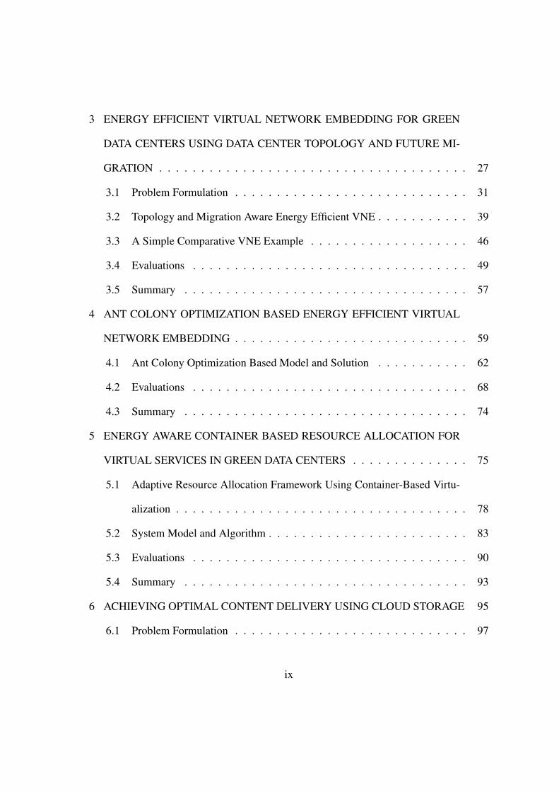
3 ENERGY EFFICIENT VIRTUAL NETWORK EMBEDDING FOR GREEN

DATA CENTERS USING DATA CENTER TOPOLOGY AND FUTURE MI-

GRATION . . . . . . . . . . . . . . . . . . . . . . . . . . . . . . . . . . . . . 27

3.1 Problem Formulation . . . . . . . . . . . . . . . . . . . . . . . . . . . . 31

3.2 Topology and Migration Aware Energy Efficient VNE . . . . . . . . . . . 39

3.3 A Simple Comparative VNE Example . . . . . . . . . . . . . . . . . . . 46

3.4 Evaluations . . . . . . . . . . . . . . . . . . . . . . . . . . . . . . . . . 49

3.5 Summary . . . . . . . . . . . . . . . . . . . . . . . . . . . . . . . . . . 57

4 ANT COLONY OPTIMIZATION BASED ENERGY EFFICIENT VIRTUAL

NETWORK EMBEDDING . . . . . . . . . . . . . . . . . . . . . . . . . . . . 59

4.1 Ant Colony Optimization Based Model and Solution . . . . . . . . . . . 62

4.2 Evaluations . . . . . . . . . . . . . . . . . . . . . . . . . . . . . . . . . 68

4.3 Summary . . . . . . . . . . . . . . . . . . . . . . . . . . . . . . . . . . 74

5 ENERGY AWARE CONTAINER BASED RESOURCE ALLOCATION FOR

VIRTUAL SERVICES IN GREEN DATA CENTERS . . . . . . . . . . . . . . 75

5.1 Adaptive Resource Allocation Framework Using Container-Based Virtu-

alization . . . . . . . . . . . . . . . . . . . . . . . . . . . . . . . . . . . 78

5.2 System Model and Algorithm . . . . . . . . . . . . . . . . . . . . . . . . 83

5.3 Evaluations . . . . . . . . . . . . . . . . . . . . . . . . . . . . . . . . . 90

5.4 Summary . . . . . . . . . . . . . . . . . . . . . . . . . . . . . . . . . . 93

6 ACHIEVING OPTIMAL CONTENT DELIVERY USING CLOUD STORAGE 95

6.1 Problem Formulation . . . . . . . . . . . . . . . . . . . . . . . . . . . . 97

ix

6.2 Approximation Algorithm . . . . . . . . . . . . . . . . . . . . . . . . . 107

6.3 Evaluations . . . . . . . . . . . . . . . . . . . . . . . . . . . . . . . . . 115

6.4 Summary . . . . . . . . . . . . . . . . . . . . . . . . . . . . . . . . . . 122

7 CONCLUSIONS AND FUTURE WORK . . . . . . . . . . . . . . . . . . . . 124

REFERENCE LIST . . . . . . . . . . . . . . . . . . . . . . . . . . . . . . . . . . 126

VITA . . . . . . . . . . . . . . . . . . . . . . . . . . . . . . . . . . . . . . . . . 143

x

ILLUSTRATIONS

Figure Page

1 PUE data for all large-scale Google data centers [116] . . . . . . . . . . . 2

2 Power consumption elements considered by Google in their power mea-

surement [116] . . . . . . . . . . . . . . . . . . . . . . . . . . . . . . . 3

3 Architecture of three types of virtualization techniques . . . . . . . . . . 8

4 An example of VNE for green DCs . . . . . . . . . . . . . . . . . . . . . 28

5 A typical hierarchical fat tree data center architecture . . . . . . . . . . . 29

6 Topology awareness reduces energy consumption (right) . . . . . . . . . 29

7 Topology Aware VNE (TA-VNE): no feasible embedding available . . . . 47

8 Migration Aware VNE (MA-VNE): total energy cost 86 units . . . . . . . 47

9 Topology and Migration-Aware Energy Efficient VNE (TMAE-VNE): to-

tal energy cost: 52 units . . . . . . . . . . . . . . . . . . . . . . . . . . . 48

10 Comparison with optimal solution . . . . . . . . . . . . . . . . . . . . . 52

11 Comparison for varied resource usage ratio . . . . . . . . . . . . . . . . 53

12 Comparison for varied number of DCs . . . . . . . . . . . . . . . . . . . 54

13 Comparison for varied number of DCs under B4 topology . . . . . . . . . 56

14 Construction graph for ACO model . . . . . . . . . . . . . . . . . . . . . 62

xi

15 A tuple (i, i′, u) in the ACO construction graph represents a mapping in

the EE-VNE problem that virtual node u is assigned to physical node i at

time t and physical node i′ at time t+ 1. . . . . . . . . . . . . . . . . . . 64

16 Comparison with optimal solution . . . . . . . . . . . . . . . . . . . . . 69

17 Comparison for varied number of DCs . . . . . . . . . . . . . . . . . . . 70

18 Impact of parameters in ACO . . . . . . . . . . . . . . . . . . . . . . . . 73

19 Hypervisor based virtual machines cannot be embedded due to resource

limitation . . . . . . . . . . . . . . . . . . . . . . . . . . . . . . . . . . 77

20 Container based virtural machines have been successfully allocated with

available resources . . . . . . . . . . . . . . . . . . . . . . . . . . . . . 78

21 Overview of adaptive resource allocation framework . . . . . . . . . . . 79

22 Components in a physical machine . . . . . . . . . . . . . . . . . . . . . 81

23 Work flow of adaptive resource allocation for activating an application . . 82

24 Comparison for varied number of physical machines . . . . . . . . . . . 92

25 Comparison for varied number of virtual machines . . . . . . . . . . . . 93

26 Push vs. pull: The origin server pushes some objects to proxy servers.

Content user queries objects from the proxy server. A proxy server will

pull from the origin server or another cooperative proxy server if it doesn’t

have the requested objects. . . . . . . . . . . . . . . . . . . . . . . . . . 97

27 ri1 = 1.33; ri2 = 1; ri3 = 0.94. Pushing object 1 and 2 with the lowest

ratio ri1 and ri2(case (a)) is worse than pushing object 3 (case (b)). . . . . 108

xii

28 In TLM, either object 1, . . . , L− 1, (L > 1) or object L can be pushed to

a proxy server. . . . . . . . . . . . . . . . . . . . . . . . . . . . . . . . . 111

29 The upper bound of optimal solution . . . . . . . . . . . . . . . . . . . . 111

30 Comparison for varied number of objects (simulation with real object sizes)116

31 Comparison for varied standard deviation of object sizes (simulation with

synthetic object sizes) . . . . . . . . . . . . . . . . . . . . . . . . . . . . 118

32 Comparison for varied balance parameter α (simulation with real object

sizes) . . . . . . . . . . . . . . . . . . . . . . . . . . . . . . . . . . . . 118

33 Locations for the origin server and proxy servers: the mark in the circle

indicates the location for the origin server; and the remain sites are all

proxy servers. Each proxy server is connected to origin server and its

cooperative proxy servers. Proxy servers may pull objects from the origin

server or a closer proxy server. . . . . . . . . . . . . . . . . . . . . . . . 120

34 Comparison for varied number of objects (Planetlab experiments with real

object sizes) . . . . . . . . . . . . . . . . . . . . . . . . . . . . . . . . . 121

35 Comparison for varied standard deviation of object sizes (Planetlab ex-

periments with synthetic object sizes) . . . . . . . . . . . . . . . . . . . 121

36 Comparison for varied balance parameter α (Planetlab experiments with

real object sizes) . . . . . . . . . . . . . . . . . . . . . . . . . . . . . . 122

xiii

TABLES

Tables Page

1 Component Peak Power Breakdown for a Typical Server [43] . . . . . . . 4

2 Network Virtualization Implementation Techniques Comparison . . . . . 10

3 Comparison of VNE Studies . . . . . . . . . . . . . . . . . . . . . . . . 20

4 Notations Used . . . . . . . . . . . . . . . . . . . . . . . . . . . . . . . 31

5 Algorithms Comparison . . . . . . . . . . . . . . . . . . . . . . . . . . . 49

6 Parameter Setting . . . . . . . . . . . . . . . . . . . . . . . . . . . . . . 51

7 Notations Used . . . . . . . . . . . . . . . . . . . . . . . . . . . . . . . 63



10 Notation Used . . . . . . . . . . . . . . . . . . . . . . . . . . . . . . . . 98

11 Parameter Setting for Simulations . . . . . . . . . . . . . . . . . . . . . 116

12 Parameter Setting for Planetlab Experiments . . . . . . . . . . . . . . . . 119

xiv

ACKNOWLEDGEMENTS

I would like to express my deepest gratitude to my advisor, Dr. Baek-Young

Choi, for her guidance, understanding, patience and full support during my Ph.D. study at

University of Missouri-Kansas City. Not only gives many helpful advises on my research

work, she also provides many invaluable opportunities and suggestions towards my long-

term career goals. She is willing to share her experiences and always encourages me to

grow as an independent researcher.

I would like to sincerely thank Dr. Sejun Song, for his inspiring guidance, tutoring

and financial support. His insights and comments were significant supports for me to un-

derstand software defined networks and to clarify and improve the cost efficient resource

allocations work presented in this dissertation.

I am grateful to other committee members of my dissertation, Dr. Cory Beard,

Dr. Deep Medhi, Dr. Ghulam Chaudhry, and Dr. Xiaojun Shen for their assistances and

suggestions. When I am facing questions, they are always open for discussion.

I would like to thank Dr. Hiroshi Saito, Dr. Ryoichi Kawahara for their mentoring

during my internship at NTT Service Integration Laboratories. I would also like to thank

my mentors Dr. Xin Wang, Dr. Jiafeng Zhu, Dr. Guoqiang Wang, and Dr. Ravi Ravindran

for their great help and suggestions during my internships at Futurewei Technologies Inc.

I also would like to thank my lab mates, Daehee Kim, Hyungbae Park, Sunae Shin

and Kaustubh Dhondge for the friendship and their suggestions for my research.

Last and most importantly, I would like to say thank you for my husband, Xili

Wan for his unconditional love, understanding, accompanying and support for my Ph.D.

study. Thanks also go to my parents and my son for their encouragement for pursuing my

Ph.D. degree.

xvi

CHAPTER 1

INTRODUCTION

As the supporting infrastructure of cloud computing services, data centers are

rapidly proliferate in recent years. Nowadays, these data centers (DC) are used to deploy

large portion of network services and provide large volumes of cost-efficient resources,

such as virtual storage (Amazon S3 [5], Dropbox [37]), virtual platform and development

tools (Microsoft Azure [100], Google Cloud Platform [91], Amazon EC2 [39]), business

applications (Salesforce [97], Workday [121]). It is reported that there were more than

500,000 DCs around the world as of December 2011 [104].

With the fast growth of DCs and services deployed on them, more and more energy

has been consumed for DC operating and maintainable. In 2010, between 1.1% and 1.5%

of the worldwide total electricity usage was consumed by DCs [70], and their energy

costs in the US doubled from 28 billion kWh to 61 billion kWh in six years, according

to [1]. In addition, the large energy consumption of DCs not only increases the cost of DC

operators, but also impacts our environment through carbon dioxide emission. In 2008,

the carbon dioxide emission by global DCs took up to 0.3% of global carbon dioxide

emission that was more than some countries, such as Argentina and Netherland [68].

This number is expected to be double in 2020 [117].

Efforts have been made for reducing DC carbon footprint from various aspects

in order to save cost and protect environments. Companies, e.g., Google and Facebook

1

Figure 1: PUE data for all large-scale Google data centers [116]

are greening their DCs through reducing power usage for cooling and other facilities

and utilizing renewable energy [51, 83]. Now their DCs have a relatively small Power

Utilization Effectiveness (PUE), approximately 1.12 [51,83]. Figure 1 [116] presents that

Google improves the PUE of all their large scale data centers. On the other hand, the low

PUE means most energy is used for computing that drives us to control computing energy

consumption as well.

1.1 Data Centers Energy Efficiency

The power consumed for DCs mainly from three components, the computing pow-

er usage, e.g., servers, switches, storage, supporting power usage, e.g., cooling, lighting,

office use, and power transfer losses. Figure 2 [116] shows the power consumption ele-

ments that are considered in Google PUE measurement.

To describe the energy efficiency of DCs, power usage effectiveness is measured

2

Figure 2: Power consumption elements considered by Google in their power measurement[116]

by:

PUE =Total DC Power Consumption

IT Equipment Power Consumption(1.1)

The global average self-reported DC PUE is approximate 1.7, according to Uptime Insti-

tute’s 2014 Data Center Survey [106]. Compared with private DCs, public DCs usually

have a low PUE. Four approaches suggested by Google [51] to improve PUE include

managing airflow [16, 81], adjusting the thermostat [14, 64], using free cooling [73, 131],

and optimizing power distribution [95]. Through these approaches, Google improves their

3

PUE from 1.23 in 2008 to 1.12 in 2015 [116]. Now, computing energy consumption in

DCs overweight energy consumption by all the other DC components. In this disserta-

tion, we focus on minimizing the power consumption for computing, especially the CPU

power consumption and network link power consumption.

1.2 Server Power Usage

Table 1: Component Peak Power Breakdown for a Typical Server [43]Component Peak Power Count Total

CPU 40 W 2 80 WMemory 9 W 4 36 W

Disk 12 W 1 12 WPCI slots 25 W 2 50 W

Motherboard 25W 1 25 WFan 10 W 1 10 W

System Total 213 W

Servers power consumption comes from multiple components such as CPU, mem-

ory, disk and so on. Fan et al. analyzed the power usages of a server in [43]. As shown in

Table 1 [43], server power utilization is dominated by CPU and memory power usage, but

power consumed by miscellaneous items, e.g., PCI slots, motherboard becomes signifi-

cant when the workload of the server drops. With energy proportional computing [49],

voltage or frequency can be adjusted according to a CPU workload, so that machines with

less jobs consume less energy. Then, power management techniques can control power

assignments to ensure that machines with light loads consume less power, while machines

with heavy loads obtain enough power. However, when a server is completely idle without

4

doing any work, it may still consume up to 50% to 70% of its peak power [13, 127]. This

’baseline power’ cannot be eliminated unless the server is turned off [27]. ’Operation

cost’ and ’operation energy consumption’ are used to describe the power consumption

for real utilization. The operation cost is approximately linear increased as the workload

rises [13, 127]. On the other hand, majority servers in DCs is under utilization. Servers

in DCs typically operate at 10% ∼ 50% of their maximum capacity most of time [43].

These large amount of under utilized servers decrease the energy efficiency because of

the baseline power consumption.

1.3 Network Service Workload Variance

Traffic and workload of most network services are highly fluctuated related to

human activities [8,50,69]. The huge differences between the peak workload and the off-

peak workload of network services add the difficulties to provision resources for the ser-

vice in advance. To guarantee Service Level Agreement (SLA), the provisioned resources

should be enough to support the peak workload of the service. When the resources are

statically provisioned based on the peak workload, a portion of resources would be idle

when the workload of the service becomes low. As stated in Section 1.2, servers under

utilization waste large amounts of energy.

A good news is that some traffic and workload are with patterns and could be

predicted in a large time scale, such as day/night and weekday/weekend [89, 92, 98]. For

example, both daily pattern and weekly pattern have been identified for PhoneFactor ser-

vice in [92] and Youtube in [50]. In these studies, day time and weekdays have more

5

traffic and heavier workload compared with midnight to early morning and weekends.

Driven by the observations, resource could be dynamic provisioned based on the pred-

icated demand workload at a planned time, so that the idle resources can be shared by

other services or switched to sleep mode.

1.4 Virtualization Techniques

As the main enabling technology for cloud computing, virtualization support-

s multi-tenant users to share computing, storage, and networking resources. Focusing

on sizeable data centers (DCs), traditional virtualization technologies are mainly for com-

puting and storage resources. However, as DCs for cloud computing rapidly grow in

numbers and geographically dispersed DCs are interconnected, network resource virtual-

ization technology becomes one of the most promising technologies for leveraging the full

potential of cloud computing. Using virtual servers and sharing the same physical servers

significantly cut off the operation cost, power consumption, carbon emission compared

with locally hosted dedicated servers [9]. Also, live migration of virtual machines [115]

allows for demanded virtual resources to be consolidated in a physical network conserv-

ing DC energy consumption.

To enable resource sharing without impacting other virtual servers sitting in the

same physical server, various virtualization techniques are developed for different pur-

poses. Basically, currently used virtualization techniques could be categorized as: full

virtualization, paravirtualization, hardware-assested virtualization and OS-level virtual-

ization.

6

Full virtualization fully simulates the underlaying hardware. In full virtualization,

binary translation is used to trap and to virtualize instructions between the virtual hard-

ware and the host computer’s hardware. Binary translation incurs a large overhead, so

that the performance of full virtualization may not be good. However, guest OS could be

directly embedded without any modification. Examples of full virtualization are VMWare

ESXi [40] and Microsoft Virtual Server [99].

Paravirtualization cannot directly embedded a guest OS without any modification.

A thin layer named Hypervisor provides API for the communication between the guest

OS and hardware. Compared with full virtualization, paravirtualization has a better per-

formance with a lower overhead, but is harder to be implemented since the guest OS need

to be tailored to run on the Hypervisor. Example of paravirtualization is Xen [85].

Hardware-assested virtualization is a type of full virtualization. In stead of binary

translation and paravirtualization, hardware handles privileged and sensitive calls that

automatically trapped to Hypervisor. Examples of hardware-assested virtualization are

Linux KVM [79], VirtualBox [20].

OS-level virtualization or container-based virtualization is an alternative to Hy-

pervisor based virtualization techniques. They are based on Linux container [102] and

provide superior system efficiency and isolation. Unlike Hypervisor based virtualization,

container based virtualization does not need to simulate the entire guest OS, but works as

a thread. Therefore, container based VMs are light weighted, and could be fast deployed

and migrated between different locations. One of management tool of container based

virtualization, named Docker [35] is widely recognized and adopted in many companies

7

as well. The advent of container based virtualization and the related management tool-

s offer a great opportunity to further improve energy efficiency and reduce cost in data

centers.

(a) Bare-metal Virtualization (b) Hosted Virtualization

(c) Container-based Virtualization

Figure 3: Architecture of three types of virtualization techniques

As shown in Figures 3, container-based virtualization does not build the guest OS,

but only adds necessary bins and libraries to support the applications, while guest OS

8

is deployed for Hypervisor based OS. In addition, in container-based virtualization, an

engine is used to coordinate among multiple containers, while Hypervisor is employed

for isolation and resource mapping.

1.5 Network Virtualization

Besides vitualization of servers, network virtualization has been studied and de-

veloped for different purposes. For example, virtual networks are utilized to adopt new

protocols or techniques for academic usage. In addition, they are employed to support

multi-tenant environments for cloud computing and widely spread data centers. By al-

lowing resource sharing, virtual networks saves a lot for service providers comparing

with traditional dedicated DCs.

Various techniques have been developed to provision virtual resources, create and

maintain virtual networks, including Virtual Local Area Networks(VLAN), Virtual Pri-

vate Networks(VPN), Overlay Networks, and Programmable Networks.

VLAN partitions ports on switches so that network traffic through tagging pack-

ets on hosts. It enables host grouping even if the hosts are not under the same switch.

Furthermore, it is flexible to migrate one host from one virtual network to another one by

simply changing its VLAN identifier.

VPN assists the construction of logical private networks over public network in-

frastructure by establishing virtual end-to-end connections using tunnelling. VPN can

be implemented at different network layer (layer 1, layer 2 and layer 3) using various

techniques.

9

Overlay networks are built on top of other networks. In overlay networks, hosts

are connected through logical links or tunnels, e.g., GRE tunnels, L2TP tunnels. Overlay

networks typically are implemented at the application layer. Examples of overlay net-

works applications include most peer to peer protocols, such as Gnutella, Tor, content

delivery networks, and real time media flow protocol. Note that VPNs can be categorized

as overlay networks.

Programmable networks are networks in which their network devices behavior

and flow control are handled independently by software rather than network hardware.

Especially software defined networks separate data plane and control plane through mov-

ing routing function from network router to controllers. By using SDN infrastructures,

network operators have a freedom in choosing the optimal physical servers and physical

paths to support virtual nodes and virtual links without interfering other network services

or functions.

Existing work, such as [38] that built FlowN, a VNE prototype on NOX OpenFlow

controller, and [96] that proposed VNE architecture using BGP configurations and Open-

Flow 1.3 switches, gives some guideline in implementing VNE using SDN architecture

and infrastructures.

Table 2: Network Virtualization Implementation Techniques ComparisonTechnique Name Implementation Layer

VLAN Link layerVPN Physical layer, link layer, network layer

Overlay networks Application layerProgrammable networks Network layer

10

1.6 Scope and Contribution of this Dissertation

This dissertation focuses improving the efficiency of cloud data centers by devel-

oping resource allocation algorithms for two different service requirements. When the

service provider explicates the desired virtual network including a specific topology, and

a set of virtual nodes with certain resource demands, the infrastructure provider computes

how the given virtual network is embedded to its operated data centers with minimum

energy consumption. We consider the evolving workload of the virtual networks or virtu-

al applications and residual resources in data centers, and build a novel model of energy

efficient virtual network embedding (EE-VNE) in order to minimize energy usage in the

physical network consists of multiple data centers. In this model, both operation cost

for executing network services’ task and migration cost for the live migrations of virtual

nodes are counted toward the total energy consumption. Two algorithms are developed

towards this optimization problem.

The other is when the service provider only gives some description about the net-

work service and the desired QoS requirements, the infrastructure provider has more free-

dom on how to allocate resources for the network service. We design a framework to

dynamically allocate resources for a network service by employing container based vir-

tual nodes. In the framework, each network service would have a pallet container and

a set of execution containers. The pallet container requests resource based on certain s-

trategy, creates execution containers with assigned resources and manage the life cycle of

the containers; while the execution containers execute the assigned job for the network

service.

11

In addition, the joint optimization for content placement problem has been studied

to minimize the traffic from content to the final content users without increasing their

experienced latency.

The main contributions of this dissertation are summarized as follows:

1) We formulate the problem of virtual network embedding that incorporates energy

costs of operation and migration for nodes and links that is non-linear. To solve this

problem, we introduce a technique to transform it to a linear programming problem

with additional constraints. After proving the NP-hardness of this problem, we de-

velop a heuristic algorithm named Topology and Migration-Aware Energy Efficient

Virtual Network Embedding (TMAE-VNE) to minimize the energy consumption

caused by both operation and future migration. This work is initially published

in [56], and later extended to a journal paper [58].

2) To achieve a better solution of EE-VNE problem, we propose a novel ACO based

topology migration-aware EE-VNE algorithm (ACO-EE-VNE) to minimize the en-

ergy consumption caused by both operation and migration. We develop a novel

pheromone update and track scheme in the ACO algorithm, so that the space com-

plexity of the ACO algorithm is substantially reduced. This work has been pub-

lished in [59]

3) We introduce the framework for container based dynamic resource allocation mech-

anism. In this framework, service providers specify their demands from service

12

level rather than infrastructure level. Physical resources would be dynamically pro-

visioned based on current workload of each network service/application. We for-

mulate the dynamic resource allocation problem as an optimization problem and

convert it as a linear programming problem and develop an efficient and scalable

algorithm to solve the dynamic resource allocation problem that could be applied

to large scale resource pools.

4) We formulate the joint traffic-latency optimization problem, and prove its NP-

completeness. We then develop an efficient light-weight approximation algorithm,

named Traffic-Latency-Minimization (TLM) algorithm, to solve the optimization

problem with theoretical provable upper bound for its performance. To limit the

frequency of updates to the origin server with local changes such as users interest-

s shift, we also extend our TLM algorithm in a distributed manner. We provide

the theoretical analysis for time complexity and space complexity of the TLM al-

gorithm. This work is initially published in [54], and extended to a journal paper

in [55].

1.7 Organization

The remainder of this dissertation is structured as follows. In Chapter 2, we review

related work about optimization in virtual network embedding and resource allocation in

cloud data centers. Chapter 3 addresses the energy efficient virtual network embedding

13

problem with evolving demands and physical resources. Chapter 4 presents how an Ant-

Colony-Optimization based algorithm is developed and applied to solve the energy effi-

cient virtual network embedding problem. Chapter 5 proposes a container based resource

allocation framework with a scalable resource allocation algorithm. In Chapter 6, we i-

dentify traffic-latency optimization problem in content delivery networks and solve it with

practical solutions. Finally, we summarize and conclude the dissertation and introduce the

future work in chapter 7.

14

CHAPTER 2

RELATED WORK

With network virtualization techniques, adopting a new technique or protocol is

much easier [32]. Vendors or infrastructure providers (InPs) do not need to purchase new

equipment to update or deploy new techniques or protocols. An existing network could be

flexibly expanded without involving much configuration work. In addition, network vir-

tualization allows a physical network to be shared and divided into several isolated virtual

networks (VNs) that consist of virtual machines (VMs) and their specified connectivities.

Each VN serves a different group of users with different requirements of computing, stor-

age, and network resources. Small institutions could have an economic option by renting

VNs from an infrastructure provider rather than building and maintaining their private

networks. Therefore, due to its benefits, network virtualization has been highlighted and

studied from many aspects, such as resource discovery [53], admission control [94], re-

source scheduling [12], security issues [82], and resource allocation that is also known as

virtual network embedding (VNE) [31, 66, 77, 130, 132].

In this chapter, we first investigate existing work about network virtualization, and

resource allocation, then we briefly discuss about content distribution optimization that

assigns storage resources to content delivery services and determines content placement

in cloud.

15

2.1 Virtual Network Embedding (VNE)

Network virtualization allows physical nodes and links to be shared by multiple

VNs. It improves the physical resource usage efficiency, reduces the cost for service

providers, and simplifies the update and deployment of new techniques or protocols [32].

As one of the essential problems in the network virtualization area, VNE has been wide-

ly studied to achieve different goals [47]. It maps VNs coming over time to a physical

network. In a real application, an InP receives a set of VN requests from the Service

Providers (SP). Each VN asks for slices of resources, including computational and net-

work resources, to provide value-added services, such as video on demand and voice-

over-IP. By properly embedding the VNs, certain optimization goals are expected to be

achieved without violating resource limitations.

Various VNE models have been proposed with different optimization goals or

constraints. Many schemes aim to increase the VN acceptance ratio that is the number

of successfully mapped VN requests to the number of total VN requests [33], or balance

the workload on physical nodes or links [132]. [33] modeled the VNE problem with a

specified location preference of the virtual nodes as a mixed integer programming prob-

lem and presented a deterministic algorithm as well as a random algorithm to solve the

problem. [132] designed an algorithm that identifies the physical node or links with max

stress and balances the workload of those nodes or links through reconfiguration.

In all of the above mentioned research, VNE has been completed in two stages.

In the first stage, all the virtual nodes have been mapped to physical nodes that satisfy

the desired demands; while in the second stage, the algorithms compute a proper physical

16

path for each virtual link in the virtual network. It is possible that a feasible mapping

cannot be found for a virtual link, since the link capacities are not considered during

the mapping of the virtual nodes. In this case, the above mentioned algorithms have to

be backtracked to the first stage and map the virtual node again, which could be time

consuming.

To improve the mapping efficiency, one-stage VNE algorithms have been pro-

posed where the related virtual links are mapped right after mapping a virtual node

[29, 62, 77, 87, 111]. In [62], constraints on delay, routing, and location were taken into

consideration in the VNE problem, and the multicommodity flow integer linear program

is used to solve the improved model. Trinh, T. et al. [111] tried to increase the profit of the

infrastructure provider and save the cost of subscribers by applying a careful overbook-

ing concept. The topology of the physical networks and virtual networks are modeled

as a directed graph in [77], and the authors present a heuristic VNE algorithm that maps

nodes and links at the same stage based on the subgraph isomorphism. [29] is inspired

by Google’s PageRank algorithm. It argued that virtual network topologies and virtual

nodes’ positions have a significant impact on VNE’s efficiency and acceptance ratio. Vir-

tual optical networks mapping to an optical network substrate was studied in [87]. The

authors formulated the problem as integer linear programming formulations and designed

a greedy randomized algorithm to solve it. [48] proposed a pre-cluster method to parti-

tion a virtual network into clusters. In this method, multiple virtual nodes within one VN

are mapped to the same physical node if there are enough available resources, so that the

traffic inside a VN could be minimized.

17

In [124], evolving VNs and physical networks are investigated. The authors also

suggested migrating embedded virtual nodes or virtual links to accommodate more VN

requests. Driven by this observation, [22] tried to minimize the VNE cost when the sub-

strate network evolves. They compared the cost differences between re-embedding the

virtual nodes or virtual links and migrating them. They solved the proposed problem with

a heuristic algorithm. The purpose of [42] is to minimize the reconfiguration cost and bal-

ancing the physical link workload. A virtual node or link lying on a congestion physical

link would be migrated to another physical node or link. The evolvement or changes of a

virtual network are random and unexpected in [22, 42, 124].

In practice, however, many changes of VN workloads are periodic due to day/night

time zone effects or weekend effects [109, 120, 128] and can be fairly well predicted [89,

98]. Meanwhile, making the data center energy efficient and protecting the environment

attracts much attention. VNE targeting energy efficiency has been recognized and studied

in [6,19,46]. Botero, J.F. et al. [19] saved the energy consumption by reducing the number

of inactive physical nodes and physical links. Fischer, A. et al. [46] described the way

to modify existing VNE algorithms towards energy efficiency without maintaining their

other performance by considering energy as a factor when mapping. Energy efficiency is

also considered in [6] that partitions and embeds virtual DCs to the substrate network that

consists of multiple DCs, so that the inter DC traffic can be reduced and DCs with relative

low PUE are used. The migration of virtual nodes and links have not been performed in

[6, 19, 46], which would lead to a lower acceptance ratio compared with VNE algorithms

that allow migration. In addition, in both [19] and [46], multiple virtual nodes from the

18

same VN could be consolidated on the same physical node to save energy; however, this

may impact the resilience of the virtual networks. On the other hand, in our model, virtual

nodes in the same VN are ensured to be mapped to different physical nodes for resilience

consideration.

The above mentioned existing work has been summarized and compared in Ta-

ble 3. All of the aforementioned work only targets a snapshot optimization where the

resource limitations and demand requirements are considered at one time. Differing from

these existing VNE solutions, our work is unique in that we holistically aim to optimize

the energy efficiency of VNE over the entire life cycle of virtual networks. We achieve

this goal by not only considering the embedding for the current moment but also schedul-

ing possible migrations for the future at the time we map a virtual network. Thus, we

can successfully minimize operation energy costs as well as possible migration costs. In

addition, most previous work models the physical network as a graph with an arbitrary

topology. This is not precise to describe intra DC networks that are usually organized in a

hierarchical topology. We consider the practical topology of physical networks in the real

world. In our model, a physical network may consist of multiple DCs, and the network

inside each DC is hierarchical.

2.2 Meta-Heuristic Algorithms in VNE Optimization

In the above mentioned work, heuristic algorithms are developed in [6, 46] to-

wards different optimization objectives, while [19] utilized CPLEX or GPLK based exact

algorithms to solve their proposed optimization problems. CPLEX or GPLK based exact

19

Table 3: Comparison of VNE Studies

Stage Static orDynamic

Objective Algorithm

[33] Two Static Increase acceptance ratio Heuristic[132] Two Dynamic Balance load Heuristic[62] One Static Minimize cost MILP

[111] One Static Increase profit and reduce cost MILP[77] One Static Minimize cost Heuristic[29] One Static Maximize revenue Heuristic[87] One Static Minimize cost Heuristic

[124] Two Dynamic Increase profit and reduce cost Heuristic[22] One Dynamic Minimize cost Heuristic[42] One Dynamic Minimize reconfiguration cost and

balance workloadHeuristic

[19] Two Static Minimize energy consumption Heuristic[46] One or Two Static Minimize energy consumption Heuristic[6] One Static Minimize energy consumption Heuristic

algorithms are expected to achieve the optimal solutions for the small scale of the prob-

lem. However, the time consumed by these exact algorithms increase significantly as the

problem size grows. On the other hand, heuristic algorithms run in polynomial time, but

can only search in a very limited solution space, resulting in a relative low quality of the

solution compared with the solutions obtained by the exact algorithms.

Heuristic algorithms are developed in [6,46] towards different optimization objec-

tives, while Botero [19] utilized a mixed integer programmer solver based exact algorithm

to solve their proposed optimization problems. Exact algorithms can achieve the optimal

solutions in small scales but are time consuming, especially when the problem size ex-

pands; while heuristic algorithms run in polynomial time but cannot approach the optimal

20

solutions in large scale problems.

Meta-heuristic algorithm offers new methods of solving large scale NP-hard op-

timization problems. It is usually inspired by natural biological behavior and includes

probabilistic global searching based on evolutions and iterative operations. As a repre-

sentative meta-heuristic algorithm, ACO has been utilized in various large scale NP-hard

combinatorial optimization problems, e.g., [114]. In [23,41], ACO has been applied to the

VNE problem to minimize the cost of VNE. They proved that the ACO based algorithm

achieve a better performance than some existing heuristic algorithms. Chang et al. [26]

aimed to minimize the energy consumption of migration using ACO based algorithm.

However, they only considered the energy consumption in one time snapshot while we

minimize the energy consumption in the VN’s entire life cycle. However, [41] focuses

on reducing the cost of physical links, while we want to improve the energy efficiency

considering both the node energy consumption as well as link energy consumption. In

addition, we minimize the energy efficiency of the entire life cycle of virtual network

requests rather than in different time snapshots as in [6, 19, 46]. By doing this, the total

energy consumption could be further saved; however, the hardness and the scale of the

problem is increased as well. In our previous work [56], a heuristic algorithm was pro-

posed that reduced the energy consumption and improved the acceptance ratio compared

with the existing algorithms. However, as most other heuristic algorithms, it has a low

approximation ratio and is inadequate in facing a large solution space.

21

2.3 Resource Allocation

To save the cost on building and maintaining a private data center, service provider-

s move their service and data to cloud infrastructure providers. To further save cost and

improve efficiency, dynamic scaling of resource management for web application and

big data computing have been studied, such as [78, 118]. Jobs are dispatched to specific

servers with web application or hadoop running in that system. Applications are organized

in a multi-tier structure and tasks are distributed through a front-end dispatcher [122].

To provider more complicated services/applications, e.g. game hosting, resources

are required to be allocated in application level. [122] targeted energy efficient resource

allocation at VM level. By embedding and migration the entire VMs, [122] improve

energy efficiency for applications that require specific environment setting. In addition,

VN level resource allocation has been studied for different objectives, such as increasing

acceptance ratio, improving energy efficiency [57,58]. In these virtual machine or virtual

network embedding studies, they all based on VM technologies that isolate VMs at the

hardware abstraction layer, e.g., using Hypervisor based virtualization.

As an alternative of hypervisor based virtualization, container based virtualization

has been proposed in [102], and attracts many attentions in recent years. As a management

tool of container based virtualization, [35] has been recognized and widely used to deploy

many network services. [91, 100] also start to support container based virtualization in

their cloud services. Due to its light weight size, prompt deployment and shipping [44],

with container based VM, it is possible to have an application level adaptive resource

allocation mechanism.

22

However, current hypervisor VM placement models and mechanisms assume 1)

physical resources are strictly allocated for each VM, 2) the amount of VM and capacity

of VM are static. While, in container based virtualization, 1) resource could be shared

based on their priority, e.g. in docker [35], 2) dynamic change the number and capac-

ity of containers, 3) the size of containers could be different based on environments of

physical machines. Considering the different requirements, a novel framework and theo-

retical model are necessary for building an adaptive resource allocation mechanism using

container based virtualiztion techniques.

2.4 Optimal Content Distribution

Content distribution algorithms aim to optimize the system performance with lim-

ited resources expressed in various metrics. It is worth noting that those content distribu-

tion techniques can be based on a P2P structure as well as on a server/client structure. [60]

investigated content distribution techniques in both CDNs and P2P networks that are u-

tilized to decrease the traffic load in backbone networks or to optimize content users’

experience by shorter end-to-end paths and delays. The motivations of existing content

distribution techniques based on CDNs or P2P networks range from improving final user-

s’ experience to compressing access cost such as link traffic. Based on the differences

on the motivations, most of the content distribution algorithms could be categorized as

’Latency-Minimization’ (LM) and ’Traffic-Minimization’ (TM).

LM algorithms mainly focus on the optimization of the total communication delay

23

from servers to clients, which is the performance perceived by clients. The average num-

ber of autonomous systems (ASes) has been utilized to indicate latency incurred in CDNs

in [67]. The authors of [67] also proposed heuristic algorithms to minimize the average

number of ASes traveled for requests. [10,11,71] attempted to reduce clients’ access costs

for retrieving contents from peers or within the access network. The access cost is related

to the distance between content users and replicas [10, 71], or it can be a general concept

involving all the costs to complete content transmissions [11]. In addition to the commu-

nication and access latency, the computational cost is studied and reduced using clustering

algorithms in [28]. The authors in [30] studied the download latency under a competitive

P2P environment, where source peers have a limited capacity of parallel connections.

They attempted to achieve minimum download time by dynamically changing the source

set of peers under a pull-based model. Similar schemes are employed in grid computing

including where distributed resources are shared through a high speed network. In [15],

data are replicated in nearby caches to final user rather than distant source to reduce data

transmission time. In [110], LSAM proxy multicast push web pages to affinity groups

for aggregated requests to offload the central server and backbone networks. Moreover,

efficient prefetching algorithms are designed in [34,93] to indicate the most probable disk

blocks and push those blocks to user nodes in advance in order to speed up data access.

TM algorithms are designed to lower the traffic volume consumed for contents

delivery, so to cut down the expenditure for cloud services. In [4], the authors saved the

traffic cost through considering the router level and AS level topologies and utilizing mul-

ticast streams. Recently, [18] addressed the issue of reducing the traffic volume for large

24

videos in CDNs. They developed heuristic algorithms for specific topologies by using

cache clusters, assuming many system parameters were constant. The study in [61] adopt-

ed various forms of local connectivity and storage for multimedia delivery in a neighbor

assisted system to reduce access link traffic. [65] studied the influence of server alloca-

tion in ISP-operated CDNs to the transmission bandwidth consumption and suggested the

properties of nodes’ topological locations that impact cache placement effectiveness in

multiple network topologies. Unified linear programming is utilized to optimal content

placement under multiple constraints in [74]. A matrix based k-means clustering strategy

is proposed in [125] to reduce total data movement in scientific cloud workflows. This

is where the replication and distribution are constrained by enforcement policies, such as

some scientific data are restricted from moving.

Other than the LM and TM algorithms, a few recent works focus on content

delivery problems over cloud-based storage. [119] decreased the storage cost by calcu-

lating and maintaining a minimal number of replicas under certain availability require-

ments. [24, 101] tried to optimize the content providers’ investment by content delivery

over multiple cloud storage providers. [21, 76] designed and implemented frameworks

to assist replica placement over cloud storage services, in order to make it possible to

optimal content delivery over cloud under diversity requirements.

Our work differs from the previous LM and TM algorithms that we collectively

consider content providers’ expenditures on traffic volume over cloud storage and content

users’ experiences. Our aim is to address the optimization problem of traffic consumption

25

and latency for large and diverse sizes of contents by a push-pull hybrid content distri-

bution strategy, where push means replicating objects on certain servers in advance, and

pull means only delivering contents that are requested by the content users.

The push-pull strategy has been implemented for content distribution earlier. [129]

analyzed a P2P pull-based streaming protocol to understand the fundamental limitations

and design an effective protocol to achieve better throughput. [45] investigated theoretic

bounds for pull-based protocol under a mesh network and explained the performance

gap. The push-pull strategy is also utilized in data aggregation fields to minimize global

communication cost in [25]. However, those push and pull hybrid protocols are designed

for P2P networks or sensor networks without considering the storage of nodes. Therefore,

they are not suitable for content distribution over cloud storage where the storage space

impacts the content providers investment.

We focus on the environments of cloud based content delivery where the content

placement can be actively controlled considering traffic volume while the latency can be

controlled under storage constraints. We develop an efficient light-weight approximation

algorithm with a provable performance bound, and time and space complexity analy-

sis. We further design a distributed version of the algorithm in which proxy servers can

determine object distribution by exchanging local information without requiring global

knowledge.

26

CHAPTER 3

ENERGY EFFICIENT VIRTUAL NETWORK EMBEDDING FOR GREEN DATA

CENTERS USING DATA CENTER TOPOLOGY AND FUTURE MIGRATION

In this Chapter, we study energy efficient virtual network embedding considering

practical DC topologies and future migration. Unlike existing work, we focus on improv-

ing energy efficiency of virtual network embedding through planning future migration as

well as initial embedding.

By migrating some virtual nodes or links to other physical nodes or links at a

planned time based on predicated VN workloads, idle servers and network elements can

be turned off to save energy. Figure 4 depicts an example where two VNs from cloud

customers A and B are embedded onto two physical DCs during the day time due to

their resource needs. At night, however, the smaller workloads permit the infrastructure

provider to combine them onto one DC or rack saving the operating costs of servers

and switches. For example, web servers could run on multiple physical servers during

the busy hours to ensure the performance but aggregated to a less number of physical

servers at night so that some idle physical servers could be turned off to save energy. This

motivates us to design a VNE scheme that saves energy and supports energy efficient DCs

by aggregating the workload to a less number of servers and turning off idle servers.

Furthermore, in most existing VNE schemes, the physical networks to embed VN

requests are modeled with random graphs. DCs are, however, typically organized in a

hierarchical fat tree architecture, as depicted in Figure 5. We consider this hierarchical

27

(a) A VNE in Green DC during day time

(b) A VNE in Green DC during night time

Figure 4: An example of VNE for green DCs

structure when modeling the VNE problem, so that VN embedding can minimize the en-

ergy consumption used by intermediate switches as well as servers, as shown in Figure 6.

We build a novel model of virtual network embedding in order to minimize energy usage

in data centers for both computing and network resources by taking practical factors into

consideration.

The main contributions of the chapter are as follows.

28

Figure 5: A typical hierarchical fat tree data center architecture

Figure 6: Topology awareness reduces energy consumption (right)

• We formulate the problem of virtual network embedding that incorporates energy

costs of operation and migration for nodes and links that is non-linear. To solve this

problem, we introduce a technique to transform it to a linear programming problem

with additional constraints.

• After proving the NP-hardness of this problem, we develop a heuristic algorithm

29

named Topology and Migration-Aware Energy Efficient Virtual Network Embed-

ding (TMAE-VNE) to minimize the energy consumption caused by both operation

and future migration. To the best of our knowledge, this work is the first to opti-

mize energy consumption over the VN’s entire life cycle, considering time varying

resource demands of virtual network requirements. In addition, we consider a prac-

tical intra-DC architecture to further improve energy efficiency.

• We conduct extensive evaluations and comparisons with two state-of-the-art algo-

rithms using various inter-DC topologies. The results show that the proposed algo-

rithm substantially saves energy consumption and allows high acceptance ratios.

The remainder of this chapter is organized as follows. We formally model the

VNE problem with dynamic VN requests, physical nodes with sleep/awake modes, and

realistic DC network topologies in Section 3.1. The proposed algorithm is described

in Section 3.2. A motivating example is discussed in Section 3.3. The performance

evaluations and comparisons of the proposed algorithm with existing algorithms using

multiple DC topologies are presented in Section 3.4. The concluding remarks of this

chapter are given in Section 3.5.

30

3.1 Problem Formulation

Table 4: Notations UsedNotation Explanation

Gp(Np, Lp) A physical network with a set of physical nodes Np

and a set of physical links Lp

Gv(N v, Lv) A virtual network with a set of virtual nodes N v and

a set of virtual links Lv

Gpinter A physical network that connects data centers

Lpinter A set of inter-DC physical links

D The number of DCs

cp(i) Total computational resources of a physical node i

cp(i, t) Available computational resources of a physical node i

at time t

cv(u, t) The desired computational resources to embed the

virtual node u at time t

wp(i, j) weight of physical link (i, j)

bp(i, j) Total bandwidth resources of the physical link

between i and j

bp(i, j, t) Available bandwidth resources of the physical link

between i and j at time t

bv(u,w, t) Desired bandwidth to map the virtual link between u

and w at time t

Ebase(i) Baseline energy consumption of the physical node i

Copr Total operation energy consumption for embedding VN

requests

Cmgr Total energy consumption of necessary migrations for

embedded VN requests

s(u, t) State information of virtual node u

at time t

x(i, u, t) Binary variable if virtual node u is embedded to physical

node i at t or not

Sstatus(i, t) Sleep or awake status of physical node i at time t

f(i, j, u, w, t) If virtual flow between virtual node u and w goes

through the link between physical node i and j at time t

31

We model the energy efficient VNE problem as an optimization problem aiming

to minimize the energy consumed for embedding VN requests. Specifically, the total

energy consumption consists of the energy consumed for operation and migration under

a group of constraints, including computational and network resource limitations, binary

limitations, and flow constraints. We further transform the proposed VNE problem to a

linear program problem by introducing two auxiliary variables.

3.1.1 Notations

In this section, we model the VNE problem that minimizes the energy consump-

tion with practical DC topologies and migration awareness. Notations used in the Chapter

3 are listed in Table 4.

Assume a physical network Gp(Np, Lp) consists of multiple DCs Gp1(N

p1 , L

p1),

Gp2(N

p2 , L

p2), · · · , Gp

D(NpD, Lp

D). Here, D is the number of DCs in a physical network. A

DC d includes a group of physical nodes Npd and physical links Lp

d. We have

Gp = Gp1

∪Gp

2

∪· · ·

∪Gp

D

∪Gp

inter

Np = Np1

∪Np

2

∪· · ·

∪Np

D

Lp = Lp1

∪Lp2

∪· · ·

∪Lp

D

∪Lpinter

where Gpinter is the network that connects DCs, and Lp

inter is the set of all inter DC links.

Each physical node i ∈ Np is equipped with limited computational resources cp(i)1, while

each physical link between two adjacent physical nodes i and j has limited bandwidth

bp(i, j).1Here, we consider a general computational resources. In real applications, it could be CPU capacity or

available storage size

32

An infrastructure provider receives VN requests and assigns proper computational

and network resources satisfying the specific demands of each VN request. In detail, a

VN request can be modeled as a weighted graph Gv(N v, Lv), where N v and Lv are the

sets of virtual nodes and virtual links, respectively.

Based on the observation that users’ workloads often change predictably with

time, such as day and night times [128], we assume VN resource workloads are differ-

ent in the time intervals. We denote the minimal desired computational resource at time

t for a virtual node u ∈ N v as cv(u, t), and the minimal desired bandwidth resource at

time t for a virtual link in Lv as bv(u,w, t). For the simplicity of our discussion, we only

consider demands of two different times (t and t + 1 for day and night times, respective-

ly, for example) for each VN request in the illustrating example and evaluation sections.

However, the idea of scheduling and mapping can be naturally extended to handle more

time intervals. For a certain virtual node u of VN request v, its requested computational

resource cv(u, ·) is specified for the day and night times as shown below.

cv(u, ·) =

{cv(u, t), during day time

cv(u, t+ 1), during night time(3.1)

The requested bandwidth between virtual nodes u and w, bv(u,w, ·) is specified for the

day and night times as:

bv(u,w, ·) =

{bv(u,w, t), during day time

bv(u,w, t+ 1), during night time(3.2)

After embedding some VN requests, the available computational resources of a

physical node i are the residual computational resources after reserving resources for

33

already embedded VN requests:

cp(i, t) = cp(i)−∑∀v↑i

cv(u, t) (3.3)

Here, v ↑ i indicates that virtual node v is embedded on physical node i. Due to the

different demands of VN requests for day and night times, the available resources change

over time too.

Similarly, the available bandwidth of a physical link between two adjacent physi-

cal nodes i and j is defined as:

bp(i, j, t) = bp(i, j)−∑

∀(u,w)↑(i,j)

bv(u,w, t) (3.4)

Here, (u,w) ↑ (i, j) indicates that the virtual link between virtual node u and w passes

through the physical link between physical nodes i and j.

Our goal is to embed a group of VN requests with minimal energy consumption

that consists of operational energy cost Copr, and migration energy cost Cmgr under re-

source limitations, which is defined as follows;

min∑t

(Copr(t) + Cmgr(t)) (3.5)

In addition, we assume that physical nodes support the sleep and awake mode in

the physical network. Especially, there is no energy consumption if a physical node is

turned to the sleep mode. For an awake node, a baseline energy is consumed for main-

taining basic functions [127], while for each newly embedded virtual node, an additional

power is consumed for performing the work on this virtual node.

34

3.1.2 Operation Energy Consumption

We model the operational energy consumption including energy costs for nodes

and links as:

Copr(t) = Energy cost for nodes + Energy cost for link bandwidths

=∑i

∑u

∑t=0

[αo1Ebase(i)Sstatus(i, t) + αo2cv(u, t)]x(i, u, t)

+αo3

∑i,j

∑u,w,u>w

∑t=0

wp(i, j)bv(u,w, t)f(i, j, u, w, t)

(3.6)

Here, a binary variable x(i, u, t) is used to indicate whether or not a virtual node

u is embedded to physical node i at time t.

x(i, u, t) =

{1, if virtual node u is assigned to physical node i at time t

0, otherwise(3.7)

The operation cost of embedding a virtual node u to physical node i at time t

consists of a possible baseline energy consumption Ebase(i) for waking up node i if its

status Sstatus(i, t − 1) at time t − 1 is asleep and an operation cost for executing virtual

node u’s tasks cv(u, t) at time t.

Sstatus(i, t) =

{1, if physical node i is asleep at the beginning of time t

0, otherwise(3.8)

On the other hand, link operation cost is determined by traffic volume, bv(u,w, t)

on the virtual link (u,w) at time t, and the weight, wp(i, j) of the physical links (i, j) that

is different for inter or intra DC links. We use network flow f(i, j, u, w, t) to determine

whether a physical link (i, j) is used to embed a virtual link u,w. When f(i, j, u, w, t)

35

is equal to 1, virtual link (u,w) passes through the physical link (i, j). Otherwise,

f(i, j, u, w, t) is equal to 0. Coefficients αo1 , αo2 , and αo3 are used to balance the weight

among different parts of the operation cost.

3.1.3 Migration Energy Consumption

Even though migrating embedded virtual nodes could save energy, it may intro-

duce additional overhead, such as the cost for moving system resources and maintaining

additional links when the migration is processed. [115] describes the processes of the vir-

tual router’s live migration and its related overhead. We model the migration energy cost

at time t as shown below.

Cmgr(t) = Cost due to size of system resource + Cost due to bandwidth usage

= αm1

∑i1,i2,i1 =i2

∑u

∑t=1

s(u, t)Elen(i1, i2)x(i1, u, t− 1)x(i2, u, t)

+ αm2

∑i1,i2,i1 =i2

∑a,b

∑u,w,u>w

∑t=1

bv(u,w, t− 1)x(i1, u, t− 1)x(i2, u, t)

f(a, b, u, w, t− 1)wp(a, b))

(3.9)

Here, we formulate the migration cost as the summation of duplicating the virtual nodes’

status and maintaining duplicated links before migration is completed. In Equations (3.9),

s(u, t) is the coefficient indicating the cost of duplicating execution status for virtual node

u at time t. Elen(i1, i2) is the weight of a physical path between physical nodes i1 and i2.

The product of x(i1, u, t−1) and x(i2, u, t) indicates that the virtual node u was embedded

on physical node i1 at time t−1 and migrated to physical node i2 at time t. bv(u,w, t−1)

36

is the coefficient for maintaining the physical link (a, b) that is used for embedding the

virtual link (u,w). Coefficients αm1 , αm2 , and αm3 are used to balance the weight among

different parts of the migration cost.

3.1.4 Transformation of the Optimization Objective

Due to the existence of the products of variables, such as x(i1, u, t− 1)x(i2, u, t),

the objective function is a non-linear problem that is hard to solve. We transform it to a

linear program problem by introducing two auxiliary binary variables: m(i1, i2, u, t− 1)

and g(i1, i2, a, b, u, w, t). Here we replace x(i1, u, t− 1)x(i2, u, t) with m(i1, i2, u, t− 1)

and replace x(i1, u, t−1)x(i2, u, t)f(a, b, u, w, t−1) with g(i1, i2, a, b, u, w, t). Intuitive-

ly, m(i1, i2, u, t − 1) indicates if a virtual node u has migrated from physical node i1 to

i2 at time t; while g(i1, i2, a, b, u, w, t) represents if a physical link (a, b) belongs to the

physical path that embedding virtual link (u,w), and one end of the virtual link has mi-

grated from physical node i1 to i2 at time t. Constraints (3.12) and (3.13) are added to

ensure the converted problem is equivalent with the original one.

The original objective function is as follows:

min (∑i

∑u

∑t=0


+αo3

∑i,j

∑u,w,u>w

∑t=0


+αm1

∑i1,i2,i1 =i2

∑u

∑t=1

s(u, t)wp(i1, i2)x(i1, u, t− 1)x(i2, u, t)

+αm2

∑i1,i2,i1 =i2

∑a,b

∑u,w,u>w

∑t=1

bv(u,w, t− 1)x(i1, u, t− 1)x(i2, u, t)

f(a, b, u, w, t− 1)))wp(i, j) (3.10)

37

The transformed objective function is as follows:

min (∑i

∑u

∑t=0


+αo3

∑i,j

∑u,w,u>w

∑t=0


+αm1

∑i1,i2,i1 =i2

∑u

∑t=1

s(u, t)wp(i1, i2)m(i1, i2, u, t)

+αm2

∑i1,i2,i1 =i2

∑a,b

∑u,w,u>w

∑t=1

bv(u,w, t− 1)g(i1, i2, a, b, u, w, t)

wp(i, j))) (3.11)

The following two constraints are introduced to ensure the equivalence of the con-

verted problem and the origin problem.

0 ≤ x(i1, u, t− 1) + x(i2, u, t)− 2m(i1, i2, u, t) ≤ 1 (3.12)

0 ≤ m(i1, i2, u, t) + f(a, b, u, w, t− 1)− 2g(i1, i2, j, a, b, u, w, t) ≤ 1 (3.13)

3.1.5 Constraints

The optimization goal is subjected to the constraints on computational and net-

work resources. ∑u

cv(u, t)x(i, u, t) ≤ cp(i, t), ∀i, t (3.14)

∑u,w

f(i, j, u, w, t)bv(u,w, t) ≤ bp(i, j, t),∀i, j, t (3.15)

Constraint (3.14) ensures that for each physical node i at any time t, the total

required computational resources of virtual nodes that mapped to i would not exceed the

available computational resources on i. Constraint (3.15) guarantees that for each physical

38

link (i, j), the total amount of bandwidth required by the virtual links would not exceed

the available bandwidth on (i, j).

Constraint (3.16) is employed to ensure that each virtual node u must be embedded

to a physical node i. ∑i

x(i, u, t) = 1,∀u, t (3.16)

Considering the resilience as in an existing VNE work, it is not allowed that two

virtual nodes from the same VN are embedded to the same physical node. Therefore, we

have ∑u

x(i, u, t) ≤ 1, ∀i, t (3.17)

Finally, flow conservation is used to make sure that the net flow of a physical node

must be zero except for the physical node that embeds a virtual node.∑j

f(i, j, u, w, t)−∑j

f(j, i, u, w, t) = x(i, u, t)− x(i, w, t), ∀i, u, w, t (3.18)

Through solving the transformed optimization problem (3.11) under a group of

constraints (3.12)-(3.18), we could obtain the optimal solution of the topology and mi-

gration aware energy efficient VNE by using IBM ILOG CPLEX or other math tools for

linear programming problems. However, due to the large solution space, time spent to

solve the problem grows exponentially when the size of the problem increases. Thus, an

efficient algorithm is necessary for computing the optimal embedding for VN requests.

3.2 Topology and Migration Aware Energy Efficient VNE

We first study the complexity of the formulated optimization problem, and prove

the NP-hardness of the TMAE-VNE problem. We next propose a heuristic algorithm

39

to determine scheduling to maximally save the total energy consumption in a scalable

manner.

3.2.1 Hardness of TMAE VNE problem

The optimization problem formulated in Section 3.1 can be shown to be NP-hard,

as a standard VNE problem which is known to be NP-hard [7] can be reduced to this in

polynomial time. A standard VNE problem is defined as below.

Standard VNE problem: Given an undirected graph Gp = (Np, Lp), a set of ver-

tices i ∈ Np and a set of edges (i, j) ∈ Lp, where i, j ∈ Np has been assigned a value

cp(i) or bp(i, j), respectively. Given another undirected graph Gv = (N v, Lv), a set of

vertices u ∈ N v and a set of edge (u,w) ∈ Lv, where u,w ∈ N v has been assigned a

value cv(i) or bv(i, j), respectively.

The problem is to determine whether or not we can find a set of valid mappings

from Lv to Lp. In each mapping from edge (u,w) ∈ Lv to (i, j) ∈ Lp, two conditions are

satisfied 1) cp(i) ≥ cv(u), and cp(j) ≥ cv(w); 2) bp(i, j) ≥ bv(i, j).

We convert our TMAE-VNE problem to a decision problem and restate it as below.

Later we demonstrate that the standard VNE problem could be reduced to this problem.

TMAE-VNE problem: Given an undirected weighted graph Gp that consists of

a set of subgraphs Gp1(N

p1 , Lp

1),Gp2(Np

2 , Lp2),· · · , Gp

D(NpD, Lp

D) and a set of edges Lpinter

connecting subgraphs. Each vertex i ∈ Npd and each edge (i, j) ∈ Lp

d

∪Lp

inter, where

i, j ∈∪

dNpd has been assigned a value cp(i, t) or bp(i, j, t), respectively at time t. Given

another undirected graph Gv = (N v, Lv). Each vertex u ∈ N v and each edge (u,w) ∈

40

Lv, where u,w ∈ N v has been assigned a value cv(i, t) or bv(i, j, t), respectively at time

t.

In addition, an embedding to a node i ∈∪

dNpd brings additional cost Copr(i, t);

and embedding on a edge (i, j) ∈ Lpd

∪Lpinter products additional cost Copr(i, j, t). Mi-

grations between nodes and edges result in additional costs Cmig(i, t) and Cmig(i, j, t),

respectively. The total energy cost could be computed according to Equations [3.5], [3.6],

and [3.9].

A valid one-to-one mapping for each node u ∈ N v to a i ∈ Np and each (u,w) ∈

Lv to (i, j) ∈ Lp should satisfy two conditions: 1) cp(i, t) ≥ cv(u, t), and cp(j, t) ≥

cv(w, t); 2) bp(i, j, t) ≥ bv(i, j, t). The problem is to determine whether or not we can

find a set of valid mappings with a cost smaller than a constant value κ.

The standard VNE could be reduced to a TMAE-VNE problem, by setting cp(i) =

cp(i, t), bp(i, j) = bp(i, j, t), cv(i) = cv(i, t), and bv(i, j) = bv(i, j, t) for all t. In addition,

let Copr(i, t) = Copr(i, j, t) = 1 and κ = n + l, where n is the size of N v and l is the

number of the edges in Gp. The reduction can be completed in polynomial time. After

this reduction, if we could find a solution for a standard VNE, it would be also a solution

for the TMAE-VNE problem and vice versa. In addition, a mapping could be validated in

polynomial time if it is a solution for the TMAE-VNE problem. Thus, the TMAE-VNE

problem is NP-complete.

41

3.2.2 The Proposed Heuristic Algorithm

We use a type of a single phase algorithm where for each virtual node, its DC

and a physical node are assigned followed by its corresponding virtual link embedding.

We first determine the set of DCs to place a virtual node at each time phase t. We then

look into these DCs and find the most proper physical nodes to embed the virtual node

in each time phase. Since the number of DCs are much less than the number of physical

nodes, we could check all the set of DCs with enough resources, and finally, find a best set

that consumes the least energy. On the other hand, the energy cost of inter DC migrations

significantly overweighs that of intra DC migrations. Therefore, we first check sets of DCs

with enough available resources and determine optimal embedding in the DC granularity,

then we look into each physical node in the selected DCs.

We next consider the order of embedding each virtual node to reduce energy con-

sumption. Due to the limitation of available resources, a physical node may not embed

multiple virtual nodes. In addition, different virtual nodes cost different amounts of ener-

gy due to different connectivities and the network workload. Thus, the order of embed-

ding virtual nodes impacts total energy consumption. We determine the embedding order

for each virtual node based on the possible saved energy if this virtual node is embedded

first. For each virtual node u, we pick two embeddings with the least and the second least

energy costs. The cost difference δu between these two costs indicates possible energy

saving if the virtual node u’s embedding with the least cost is applied. Thus, we prefer to

first embed the virtual node with the largest cost difference.

The detailed algorithm is shown in Algorithm 1. For simplicity, we only consider

42

two time phases, time tday and tnight in the algorithm. In each of these time phases, the

workloads of the physical networks and VNs are different. However, our algorithm could

be easily extended for multiple time phases.

Algorithm 1 Topology and Migration-Aware Energy Efficient VNE (TMAE-VNE)Input: physical network available resources [Gp(Np, Lp), {cpi , i ∈ Np}, {bpij, i, j ∈ Np}];VN requested resources [Gv(N v, Lv), {cvu : u ∈ N v}, {bvuw : u,w ∈ N v}]Output: VNE for Gv at [t, t+ 1]

1: while there is at least one unembedded virtual node do

2: for each unembedded virtual node u do

3: ListuDC := FindFeasibleDCSets(DC, u)

4: for each element [DCd, DCd′ ] in ListuDC do

5: Estimate the total energy consumption if embedding u to DCd at time t and

DCd′ at time t+1 according to Equations (3.5), (3.6) and (3.9) based on usage,

distance to embedded virtual node and other factors

6: Record the energy consumption as Cu(DCd, DCd′)}7: end for

8: Compute δu := SecondMin{Cu} −Min{Cu}9: end for

10: virtual node w:= maxu{δu}11: Find Min{Cw} and corresponding [DCd, DCd′ ] with minimal energy consumption

in Cw(DCd, DCd′)

12: Assign w to a physical node i ∈ DCd during time t according to first fit police

while considering topology

13: Assign w to a physical nodes j ∈ DCd′ during time t+ 1 that first fit w

14: Assign virtual links whose two ends have both embedded using shortest path that

satisfy the bandwidth constraints

15: Update available resources in Gp

16: end while

43

Algorithm 2 Find Feasible DC Sets: FindFeasibleDCSets()Input: physical network available resources [Gp(Np, Lp), {cpi , i ∈ Np}, {bpij, i, j ∈ Np}],a virtual node and requested resources [u, cvu, b

vu]

Output: ListuDC

1: for each DCd, d ∈ {1, 2, . . . , D} do

2: Count DCd{np(saw, t), np(sas, t), v

p(saw, t}3: end for

4: for each time interval t for embedding do

5: for each DCd, d ∈ {1, 2, . . . , D} do

6: if np(saw, t) > 0 and vp(saw, t) ≥ cv(u, t) then

7: ListawakeDC (t) := Listawake

DC (t).append(DCd)

8: else if np(sas, t) > 0 then

9: ListasleepDC (t) := ListasleepDC (t).append(DCd)

10: end if

11: end for

12: end for

13: Ut = (ListawakeDC (t))

∪(ListasleepDC (t))

14: Ut+1 = (ListawakeDC (t+ 1))

∪(ListasleepDC (t+ 1))

15: for each DCd in Ut do

16: for each DC ′d in Ut+1 do

17: ListuDC=ListuDC .append(DCd, DC ′d)

18: end for

19: end for

As demonstrated in Algorithm 1, the physical network, the VNs along with their

topologies and available/required resources are listed as input. In steps 1-3, we count

np(saw, t) and np(sas, t), the number of physical nodes that are awake or asleep, respec-

tively, and vp(saw, t), the maximum available resources on a single awake physical node.

44

This information will help to quickly filter out DCs without enough resources. Then for

each unmapped virtual node u, we call FindFeasibleDCSets(DC,u) to calculate and

return all feasible DCs for u, ListuDC satisfying the computational resource requirements.

In the function FindFeasibleDCSets, as presented in Algorithm 2, we check

each DCd for each time phase t to see 1) if DCd has any awake physical node at time

t; 2) if vp(saw, t) is larger than the required resources of the virtual node at time t; 3)

if DCd has any asleep physical node at time t. If conditions 1) and 2) stand, d will

be added into ListawakeDC (t); or if 3) stands but not 1) or 2), DCd will be appended into

ListasleepDC (t). The union Ut of ListawakeDC (t) and ListasleepDC (t) contains all the DCs that have

enough computational resources to embed u at time t. The Cartesian product of set Ut

and Ut+1 contains all the feasible DC sets that u could be embedded into without violating

computational resource limitations.

For each element (DCd, DCd′) in ListuDC , we could roughly estimate the ener-

gy consumption Cu(DCd, DCd′) by embedding u in DCd at time t and in DCd′ at time

t + 1 using Equations (3.6) and (3.9). Each virtual node u may have multiple feasible

DC sets with different estimates of energy consumption. We pick the two DC sets with

the smallest estimated energy consumption and compute the difference δu between their

consumptions. Virtual nodes are embedded based on δ and the virtual node w with largest

δw will be embedded first. Different policies could be employed, e.g., first fit, load bal-

ance, or threshold, when embedding virtual nodes to physical nodes. After embedding

w, each virtual link connecting w and its embedded virtual neighbors will be embedded

to a physical link with the shortest path under resource constraints. Finally, the resources

45

usage is updated before embedding the next virtual node.

By calling Algorithm 2 whose time complexity is O(m), where m is the number

of physical nodes, the time complexity of Algorithm 1 is O(n2m), where n is the number

of virtual nodes in the virtual network. It is because we need to go through each phys-

ical node for the amount of available resources. However, since the number of virtual

nodes are quite small compared with the number of physical nodes, e.g., only 12 DCs are

involved in B4 [63], this algorithm is efficient and reasonable in practice.

3.3 A Simple Comparative VNE Example

In this section, we discuss an example that compares the proposed TMAE-VNE

with other existing schemes such as Topology Aware VNE (TA-VNE) [29] and Migration

Aware VNE (MA-VNE) [22]. TA-VNE embeds virtual nodes based on the static rank

that is determined by available resources and network topology. MA-VNE and TMAE-

VNE are also topology-aware as they consider the distance between physical nodes while

embedding or migrating virtual nodes or links. TMAE-VNE, on the other hand, schedules

migrations according to predictable changes of physical networks or the workload of VNs

before embedding VN requests. Therefore, migrations over an unnecessary long distance

could be avoidable. In addition, TMAE-VNE could recognize the different energy usage

between inter and intra DC links. Thus, it is especially suitable for networks of multiple

DCs. TMAE-VNE also explores an efficient DC architecture and is aware of switch

usage. The comparison of the three algorithms is summarized in Table 5.

We compare the algorithms with a simple VNE example shown in Figures 7, 8,

46

Figure 7: Topology Aware VNE (TA-VNE): no feasible embedding available

Figure 8: Migration Aware VNE (MA-VNE): total energy cost 86 units

and 9. We want to embed a VN request (with virtual nodes a and b) to a physical network

that consists of two DCs. Each DC has a gateway switch, labeled as ’SW’ and is connected

to three physical nodes. We use a pair of numbers [cp(tday), cp(tnight)] to indicate the

’available’ resource of a physical node or link during time tday and tnight. For a VN request

shown on the top, we specify the amount of ’required’ resources of the virtual node (or

link) at time tday and tnight by [cv(tday), cv(tnight)]. We assume that the operation energy

consumption for a physical link between two DCs is 10 units, while energy consumption

for a link within a single DC is 5 units. We also assume that the baseline energy for waking

47

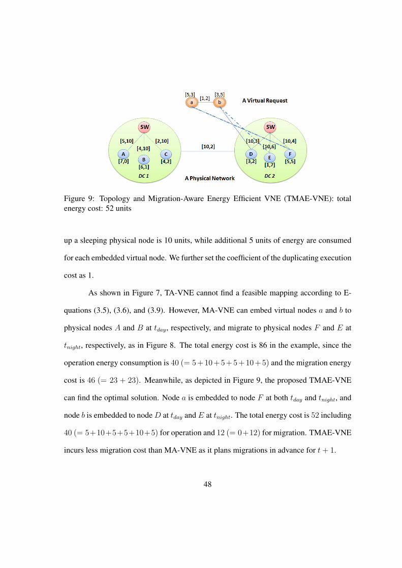
Figure 9: Topology and Migration-Aware Energy Efficient VNE (TMAE-VNE): totalenergy cost: 52 units

up a sleeping physical node is 10 units, while additional 5 units of energy are consumed

for each embedded virtual node. We further set the coefficient of the duplicating execution

cost as 1.

As shown in Figure 7, TA-VNE cannot find a feasible mapping according to E-

quations (3.5), (3.6), and (3.9). However, MA-VNE can embed virtual nodes a and b to

physical nodes A and B at tday, respectively, and migrate to physical nodes F and E at

tnight, respectively, as in Figure 8. The total energy cost is 86 in the example, since the

operation energy consumption is 40 (= 5+10+5+5+10+5) and the migration energy

cost is 46 (= 23 + 23). Meanwhile, as depicted in Figure 9, the proposed TMAE-VNE

can find the optimal solution. Node a is embedded to node F at both tday and tnight, and

node b is embedded to node D at tday and E at tnight. The total energy cost is 52 including

40 (= 5+10+5+5+10+5) for operation and 12 (= 0+12) for migration. TMAE-VNE

incurs less migration cost than MA-VNE as it plans migrations in advance for t+ 1.

48

Table 5: Algorithms ComparisonTopology Migration DC Multiple

Consideration Consideration Architecture DCs

TA Node rank # # #MA Migration When physical

distance network evolves # #TMAE Inter/Intra Physical/virtual

DC topology workload changes ! !

3.4 Evaluations

We compare the performance of TMAE-VNE with two existing algorithms, the

Topology Aware VNE (TA-VNE) [29] and Migration Aware VNE (MA-VNE) [22], with

respect to energy consumption and acceptance ratio using various parameter settings.

3.4.1 Setting

We generate a physical network that consists of DCs and links between DCs. The

inter-DC network is randomly generated using NetworkX [86], and the DCs are highly

connected through this inter-DC network. Networks within a DC are generated in a hierar-

chical architecture. Since we are focusing on VNE, we use the simplest DC architecture;

however, TMAE-VNE could be easily extended for more complicated architectures, such

as [3] to improve the scalability. A root switch connects with all aggravate switches.

Each aggregate switch is connected with a group of edge switches, and each edge switch

is connected with a group of physical nodes. The number of physical nodes in a DC is

randomly determined.

49

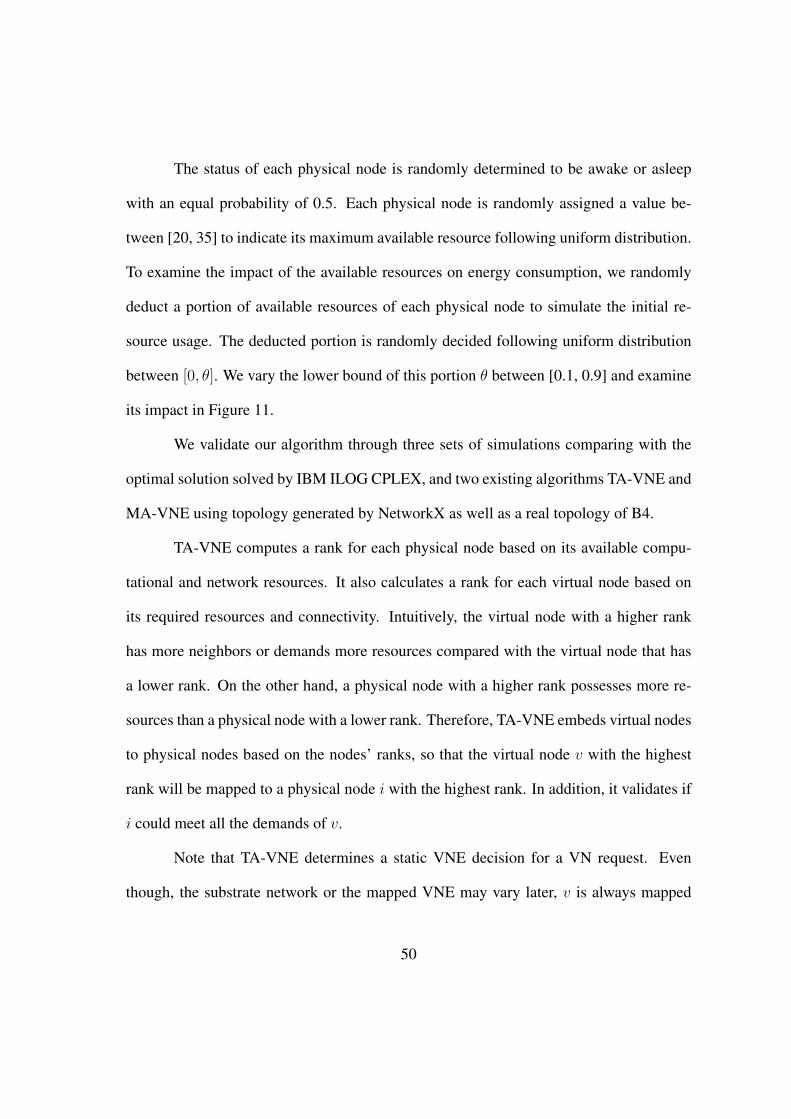
The status of each physical node is randomly determined to be awake or asleep

with an equal probability of 0.5. Each physical node is randomly assigned a value be-

tween [20, 35] to indicate its maximum available resource following uniform distribution.

To examine the impact of the available resources on energy consumption, we randomly

deduct a portion of available resources of each physical node to simulate the initial re-

source usage. The deducted portion is randomly decided following uniform distribution

between [0, θ]. We vary the lower bound of this portion θ between [0.1, 0.9] and examine

its impact in Figure 11.

We validate our algorithm through three sets of simulations comparing with the

optimal solution solved by IBM ILOG CPLEX, and two existing algorithms TA-VNE and

MA-VNE using topology generated by NetworkX as well as a real topology of B4.

TA-VNE computes a rank for each physical node based on its available compu-

tational and network resources. It also calculates a rank for each virtual node based on

its required resources and connectivity. Intuitively, the virtual node with a higher rank

has more neighbors or demands more resources compared with the virtual node that has

a lower rank. On the other hand, a physical node with a higher rank possesses more re-

sources than a physical node with a lower rank. Therefore, TA-VNE embeds virtual nodes

to physical nodes based on the nodes’ ranks, so that the virtual node v with the highest

rank will be mapped to a physical node i with the highest rank. In addition, it validates if

i could meet all the demands of v.

Note that TA-VNE determines a static VNE decision for a VN request. Even

though, the substrate network or the mapped VNE may vary later, v is always mapped

50

to i. As illustrated in Section 3.1, static VNE methods may not find the most efficient

solution or even a feasible solution. Unlike TA-VNE, MA-VNE provides a dynamic VNE

solution. When the substrate network evolves, MA-VNE may migrate a virtual node v

from a physical node i to another physical node j to save costs and increase the acceptance

ratio. In addition, delays are considered, so that v will be migrated to j only if the delay

between i and j satisfies some constraints.

We summarize the parameters used in this chapter in Table 6.

Table 6: Parameter SettingParameter Values

Probability of sleep/awake status 0.5Range for physical capacity [25, 30]

Portion of available physical resources [0.1, 0.9]Number of DCs [2, 5] or [1, 13]Size of each DC [3,6] or [5,10]

Number of hierarchy layers in each DC 3Size of VNs [3,6] or [3,10]

Amount of virtual resource request [3,5]

3.4.2 Comparison with the Optimal Solution

We first validate our algorithm by comparing it with the optimal solution solved by

IBM ILOG CPLEX. Due to the hardness of the problem, we use small physical networks

and VN requests. The number of DCs in this set of evaluations changes from 2 to 5,

while the number of physical nodes in a DC is randomly decided between 3 to 6. We also

use NetworkX to generate a random topology for each VN request. The number of virtual

nodes in each VN request is randomly selected from 3 to 6 following uniform distribution.

51

2 3 4 50

500

1000

Number of Data Centers

Com

putin

g T

ime

(s)

TA−VNEMA−VNETMAE−VNEoptimal

2 3 4 5

100

200

300

400


Tot

al E

nerg

y C

ost


2 3 4 50

50

100


Acc

epta

nce

Rat

io(%

)


(a) Execution time (b) Total energy cost (c) Acceptance ratio

Figure 10: Comparison with optimal solution

Each virtual node requires a random amount of resources between [3,5].

As presented in Figure 16(a), the average computing time of embedding each VN

by using CPLEX increases exponentially from 7.8 s to 985.03 s when the number of

DCs in the physical network rises from 2 to 5, while the computing time of TA-VNE,

MA-VNE, and the proposed TMAE-VNE are stable around 0.01 s even when the size of

the problem increases. Although there is some distance between the proposed TMAE-

VNE and the optimal solution in the total cost (Figure 16(b)) and the acceptance ratio

(Figure 16(c)), TMAE-VNE always outperforms TA-VNE and MA-VNE. As the problem

size increases, the distance between the total costs computed by the optimal solution and

that computed by the heuristic algorithms becomes larger as shown in Figure 16(b). In

addition, as shown in Figure 16(c), when the physical network expands, the acceptance

ratios of all the four methods increase as there are more available resources.

52

0.1 0.3 0.5 0.7 0.9200

250

300

350

400

Average Resource Usage

Tot

al E

nerg

y C

ost

TA−VNEMA−VNETMAE−VNE

0.1 0.3 0.5 0.7 0.90

100

200

300

400


Ope

ratio

n E

nerg

y C

ost


(a) Total energy cost (b) Operation energy cost

0.1 0.3 0.5 0.7 0.90

20

40

60


Mig

ratio

n E

nerg

y C

ost


0.1 0.3 0.5 0.7 0.90

50

100


Acc

epta

nce

Rat

io(%

)


(c) Migration energy cost (d) Acceptance ratio

Figure 11: Comparison for varied resource usage ratio

3.4.3 Comparison with Two Existing Algorithms

Using larger scale DCs, we compare our TMAE-VNE algorithm with two existing

algorithms. The number of physical nodes in a DC is randomly decided between 5 and

10, and the number of virtual nodes in each VN request is randomly selected from 3 to 10

following uniform distribution.

We examine the impact of the initial usage rate of each physical node in Figure 11

53

1 3 5 7 9 11 13

200

400

600

800


Tot

al E

nerg

y C

ost TA−VNE

MA−VNETMAE−VNE

1 3 5 7 9 11 13

200

400

600

800


Ope

ratio

n E

nerg

y C

ost



1 3 5 7 9 11 130

20

40

60


Mig

ratio

n E

nerg

y C

ost


1 3 5 7 9 11 130

50

100


Acc

epta

nce

Rat

io(%

)



Figure 12: Comparison for varied number of DCs

on the total energy cost, operation energy cost, migration energy cost, and VNE accep-

tance ratio. The average initial usage rate varies between [0.1, 0.9]. A smaller rate means

more available resources on a single physical node.

As demonstrated in Figure 11, TMAE-VNE achieves the largest acceptance ratio

and the smallest total energy consumption. When the initial usage rate increases from

0.1 to 0.9, the acceptance ratio of TMAE-VNE drops from 97.6% to 71.9%. However,

it is still 33.2% or 57% higher than TA-VNE (only 37.1%) or MA-VNE (only 14.9%),

54

respectively. The migration energy cost and operation energy cost slightly increase when

the initial usage rate grows. Since the initial usage rate is larger, physical nodes with suffi-

cient available resources are spread around the physical network. However, TMAE-VNE

always consumes the least cost. It even cuts up to 40% energy consumption compared to

MA-VNE.

We also check the impact of the number of DCs in the physical network in Figure

17. Here, the number of DCs varies from 1 to 13. When the number of DCs increase,

the total number of physical nodes that are possible to have enough capacity rises too.

However, since the network expands, the length of a physical path that embeds a virtual

link may become longer. Therefore, the total energy consumption increases when the

number of DCs increases from 1 to 3. When the physical network grows from 3 to 13, the

available resources become even more, so that TMAE-VNE could always find mappings

consuming less energy. This leads to the stable energy usage when the number of DCs is

from 3 to 13 or even a little drop from 9 to 11.

As shown in Figure 17, the acceptance ratio rises when the number of DCs in-

creases as there are more physical nodes in the entire physical network. At the same

time, migration energy costs and operation energy costs rise when the number of DCs

increases from 1 to 5 and keep stable when there are more than 7 DCs. TMAE-VNE still

consumes the least energy all the time. The acceptance ratio of TMAE-VNE is slightly

lower than MA-VNE when the number of DCs is less than 7, but it grows quickly when

there are more DCs in a physical network. This is because we determine the order for

each virtual node based on energy savings, while MA-VNE determines the order based

55

0.1 0.3 0.5 0.7 0.9300

400

500

600

700


Tot

al E

nerg

y C

ost


0.1 0.3 0.5 0.7 0.9300

400

500

600

700


Ope

ratio

n E

nerg

y C

ost



0.1 0.3 0.5 0.7 0.90

20

40

60


Mig

ratio

n E

nerg

y C

ost


0.1 0.3 0.5 0.7 0.960

70

80

90

100


Acc

epta

nce

Rat

io(%

)



Figure 13: Comparison for varied number of DCs under B4 topology

on the required resources of a virtual node. When the number of available physical nodes

is small, MA-VNE ensures the virtual nodes that require more resources are mapped first,

then it embeds the virtual nodes with a small requirement to fill the gap. However, our

TMAE-VNE could always achieve minimal energy consumption and a high acceptance

ratio as the physical network expands.

We also validate the efficiency of the TMAE-VNE algorithm using a real topology

of B4 that is a globally-deployed software defined network operated by Google [63]. B4

56

has 12 DCs covering 3 continents.

We checked the impact of the initial resource usage rate in the B4 network in Fig-

ure 13. As shown in Figure 13(a) TMAE could reduce up to 44% of the total energy

consumption compared with TA-VNE by finding a good balance between the operation

energy cost and the migration energy cost. In addition, TMAE also increases the accep-

tance ratio up to 33%. In addition, MA-VNE has the lowest acceptance ratio when the

available resources in the physical network is relative low. This is because that MA-VNE

only migrates the virtual nodes or links when their embedded physical nodes or links do

not have enough physical resources, and MA-VNE puts some limitations on the migration

distance. However, when the available resources in the physical network are extremely

(0.9), the acceptance ratio is around 90% that is better than the case that the initial resource

usage is relative low (0.7). It is because, when the available resources are extremely low,

most virtual nodes have to be migrated, and the constraint cover set would be larger.

3.5 Summary

We have modeled and proposed an efficient and practical virtual network em-

bedding algorithm (TMAE-VNE) that takes energy consumption, future migration, and

practical intra/inter DC topologies into consideration to minimize the energy consumption

caused by both operation and migration of virtual networks. Since computing and network

demands of a virtual network change over time and are often predictable (such as during

day/night times and weekday/weekends), by considering future resource migration at the

time when the different resource amounts are demanded, we have shown more physical

57

nodes and links can be put into a sleep mode leading to greater energy savings. Under-

standing hierarchical fat tree DC architectures further allows us to optimize the network

resource usages. We have performed extensive comparisons with prior VNE algorithms

using practical intra and inter-DC topologies, and we have validated that the proposed

algorithm significantly saves energy consumption, while achieving high acceptance ratios

under various scenarios.

58

CHAPTER 4

ANT COLONY OPTIMIZATION BASED ENERGY EFFICIENT VIRTUAL

NETWORK EMBEDDING

Efforts have been done to lower energy consumption by data centers, such as, pro-

portional energy consumption hardware, dynamic provisioning, and virtualization tech-

niques. Especially, Energy efficient virtual network embedding (EE-VNE) has been stud-

ied to improve the utilization of network resources and save energy consumption in data

centers in Chapter 3. However, the problem has been proved to be NP-hard. Especially,

when considering multiple data centers with evolving virtual network resources require-

ments, it becomes much more challenging to approach an optimal solution in a reasonable

amount of time.

Exact optimization algorithms with CPLEX/GLPK have been adapted to solve the

EE-VNE problem, e.g., [19]. However, as the size of the problem increases, their compu-

tation time increases dramatically. In Chapter 3, we proposed a topology and migration

aware energy efficient VNE model that aims to maximize energy savings for virtual net-

work requests during their entire life cycle rather than a time snapshot. Considering the

entire life cycle of virtual network requests further reduces the energy consumption in

VNE. However, it significantly expands the solution space compared with existing VNE

problems and leads to exponential increasing execution time. A heuristic algorithm has

been developed to solve the energy efficient VNE problem. It outperforms existing al-

gorithms in energy savings and acceptance ratios, but still cannot achieve the optimal

59

solution as we examined with simulations in Section 4.2.

A meta-heuristic method is a sophisticated tool to solve a wide group of hard

problems [17]. It provides us an alternative way to obtain near optimal solutions in a

reasonable time, especially for NP-hard problems. It has been applied to a wide group

of difficult problems [17]. Compared to heuristic algorithms and exact algorithms, meta-

heuristic algorithms could obtain high quality solutions of difficult optimization problems

in a reasonable time [108]. Driven by this, we propose an Ant Colony Optimization (A-

CO) based algorithm to solve the EE-VNE problem to minimize the energy consumption

of virtual networks during their entire life cycle rather than a time snapshot. In our mod-

el, we consider large scale physical networks and evolved virtual network requests, and

include both the operation cost and migration cost for embedded nodes and links.

In addition, we design an efficient method to track and update the pheromone to

tackle the EE-VNE problem on a large scale. Specifically, we only track and update the

pheromone on the trails that are touched by the ants. This way, the space complexity of

tracking and updating the pheromone is reduced from O(n4m2) to O(m2nantnit) where

n is the number of physical nodes; m is the number of virtual nodes; nant is the number

of ants; and nit is the number of maximum iterations. Our extensive evaluation results

show that our ACO-EE-VNE could reduce energy consumption up to 52% and double the

acceptance ratio compared with existing virtual network embedding algorithms.

The contributions achieved in Chapter 4 are as follows.

60

• We propose a novel ACO based topology migration-aware EE-VNE algorithm (ACO-

EE-VNE) to minimize the energy consumption caused by both operation and mi-

gration that provides high quality solutions without taking too much time. In doing

so, we consider data center network topologies and dynamic resource demand over

time.

• We develop a novel pheromone update and track scheme in the ACO algorithm, so

that the space complexity of the ACO algorithm is substantially reduced.

• We conduct extensive comparisons with three state-of-the-art algorithms as well as

an exact optimization algorithm using CPLEX with various inter-DC topologies.

The results prove that the proposed algorithm significantly saves energy consump-

tion and allows high acceptance ratios within a reasonable amount of execution

time.

The remainder of this chapter is organized as follows. We convert the EE-VNE

problem presented in Section 3.1 to an ACO construction graph and propose the ACO

based topology migration-aware EE-VNE algorithm in Section 4.1. We validate the per-

formance of ACO-EE-VNE algorithm through evaluations and comparisons with existing

algorithms in Section 4.2, and present the concluding remarks of this chapter in Sec-

tion 4.3.

61

Figure 14: Construction graph for ACO model

4.1 Ant Colony Optimization Based Model and Solution

In this section, we establish a construction graph similar to [36] to model our EE-

VNE problem as an ACO problem. We then design the strategies for the pheromone and

heuristic factor assignment on the tuples and links in the graph. Based on the construction

graph, and heuristic and pheromone strategies, we develop an ACO based EE-VNE algo-

rithm. Furthermore, to deal with the large scale EE-VNE problem, we propose a novel

way to track and update the pheromone on the links in the graph. Notations used in this

section are listed in Table 7.

4.1.1 ACO Model

In order to map the VNE problem to a problem that could be solved by ACO,

we build a construction graph GACO(NACO, LACO). In the graph, the embedding from

virtual nodes to physical nodes at different times are represented as tuples in the graph.

62

Table 7: Notations UsedNotation Explanation

GACO(NACO, LACO) ACO Construction graph with a set ofvertices NACO and a set of linksLACO

(i, i′, u) A vertex in ACO graph indicating thatvirtual node u is embedded to physical nodei at time t and i′ at time t+ 1

τi,i′,u,j,j′,v Pheromone on the trail between ACOvertices (i, i′, u) and (j, j′, v)

τ0 Initial pheromone that is identicalfor every trail

τi,i′,u Pheromone factor of a vertex (i, i′, u)ξ Pheromone evaporation coefficient∆k

τ Amount of pheromone laid by the kth antgbest Energy consumption of the global best

solutiongk Energy consumption of the solution found

by the kth antρki,i′,u Transition probability of ant k travels to

vertices (i, i′, u) when it has a particalsolution Sk

Ci,i′,u Total energy consumption of the assignment(i, i′, u)

The link between any two tuples A and B indicates the likelihood that an artificial ant

would move toward the tuple B when it is standing at tuple A. This likelihood is computed

based on both heuristic factor and a historical factor, pheromone. Pheromone would be

updated based on the energy consumption of solutions in previous iterations, and it would

eventually evaporate in time.

Construction graph: The vertex set NACO of GACO consists of the tuple vertex

63

Figure 15: A tuple (i, i′, u) in the ACO construction graph represents a mapping in theEE-VNE problem that virtual node u is assigned to physical node i at time t and physicalnode i′ at time t+ 1.

(i, i′, u), the nest of ants denoted by Start vertex, and the food denoted by end vertex as

shown in Figure 14. Each tuple (i, i′, u) represents a mapping from a virtual node u to

physical nodes i, i′ at different time snapshots as presented in Figure 15. Each vertex in

NACO is associated with a cost that corresponds to the energy consumption of the node

mapping including the node operation energy cost and the node migration energy cost.

LACO is the edge set of the complete graph on NACO. A link in LACO that connects

vertices (i, i′, u) and (j, j′, v) is associated with a cost that corresponds to the link energy

consumption including the link operation cost and link migration cost. If virtual nodes

u and v are not directly connected in a VN request, the cost of the link between vertices

(i, i′, u) and (j, j′, v) is set to infinite.

A trail from the nest Start to the food end corresponds to a feasible solution to

the EE-VNE problem. In this graph, ants want to find a trail from the nest start to the

food end with the minimum total cost that corresponds to the energy consumption of

64

embedding a virtual network.

Constraints: Each virtual node must be exactly mapped to one physical node at

each time slot, and each physical node cannot embed more than one virtual node for a sin-

gle VN request at any time. In addition, the mapping is subjected to resource limitations

on physical nodes and links.

Pheromone trails: The pheromone trail between any two vertices (i, i′, u) and

(j, j′, v) refers to the desirability of embedding virtual node u to physical nodes (i, i′)

while virtual node v is embedded to physical nodes (j, j′), or vice versa. The initial value

of pheromone τ0 on each trail is identical when constructing the graph. Each iteration,

pheromone on each trail evaporates as:

τi,i′,u,j,j′,v = max{τ0, (1− ξ)τi,i′,u,j,j′,v} (4.1)

where ξ is the evaporation coefficient. Meanwhile, ant k lays pheromone on the trails

between any pair of vertices in its corresponding as

τi,i′,u,j,j′,v = τi,i′,u,j,j′,v + ξ∆kτ (4.2)

∆kτ is the amount of pheromone laid by the kth ant. Here, we model ∆k

τ as the ratio be-

tween the energy consumption of the global best solution gbest to the energy consumption

of the solution gk found by the kth ant.

∆kτ =

gbestgk

(4.3)

We denote the set of already traveled vertices by the kth ant as partial solution Sk.

For the kth ant, the pheromone factor τi,i′,u of a vertex (i, i′, u) depends on the quantity of

65

pheromone on the edges between the vertex (i, i′, u) and the vertices in Sk:

τi,i′,u =∑

(j,j′,v)∈Sk

τi,i′,u,j,j′,v (4.4)

Heuristic information: The ratio between the minimum possible node energy con-

sumption 2χop to the energy consumption Ci,i′,u of mapping the virtual node u are utilized

as the heuristic factor ηi,i′,u

ηi,i′,u =χopr

Ci,i′,u(4.5)

χopr =∑t

αo2cv(u, t) (4.6)

We use the operation power consumption χopr of a physical node multiply the length of

the operation time duration 2, as the minimum possible node embedding energy consump-

tion, and compute the energy consumption Ci,i′,u as the sum of node operation energy

consumption Copr(i, i′, u), defined in Equ. (3.6) and node migration energy consumption

Cmgr(i, i′, u), defined in Equ. (3.9).

Ci,i′,u = Copr(i, i′, u) + Cmgr(i, i

′, u) (4.7)

Based on the heuristic factor ηi,i′,u and pheromone factor τi,i′,u of each vertex,

each ant selects vertices randomly within the candidate set with respect to the transition

probability ρi,i′,u when the kth ant has a partial solution Sk, i.e.,

ρki,i′,u =[ηi,i′,u]

α[τi,i′,u]β∑

(j,j′,v)∈Scand[ηj,j′,v]α[τj,j′,v]β

(4.8)

4.1.2 ACO-VNE

Based on the model described in Section 4.1.1, a trail from the nest start to

the food end corresponds to a solution of the EE-VNE problem. Each ant moves from

66

Algorithm 3 Ant Colony Optimization based EE-VNE (ACO-EE-VNE)

1: Build the construction graph [Gaco(Naco, Laco)], initialize the global best solutiongglobal = +∞

2: Compute the heuristic factor for each node in Naco

3: while the maximum number of iteration is not reached do4: Initialize a group of nant ants5: for Each ant do6: Call Algorithm 4 to compute the mapping results gant7: Update the pheromone matrix on the trails that have been touched using Eq.

(4.2)8: end for9: Compute the local best solution glocal in this iteration

10: if glocal < gglobal then11: Update global best solution gglobal = glocal12: end if13: Evaporate pheromone using Eq. (4.1)14: end while

one vertex to another vertex using a decision policy based on the heuristic factor and

pheromone until it eventually arrives at the food. In order to converge toward the opti-

mal solution, the algorithm runs for multiple iterations and in each iteration, multiple ants

move independently toward the food. The ants in previous iterations lay pheromone for

ants in later iterations, while the pheromone laid on each link evaporates in each iteration.

The detailed procedure of the ACO algorithm is presented in Algorithm 3 and Algorithm

4.

Note that in ACO, the pheromone on links between any two vertices are kept for

computing transition probability. The space complexity of tracking the pheromone is

O(n4m2), where n is the number of physical nodes, and m is the number of virtual nodes.

This consumes huge amounts of memory for large scale physical networks. Actually,

ants only visit a portion of the graph, and most of the links in the graph are not touched.

67

Algorithm 4 Ant Colony Optimization based EE-VNE - Solver1: Randomly choose a start vertex based on the transition probability matrix2: Put the selected vertex into trail, label corresponding physical node and virtual node

as mapped3: Put the virtual nodes that are not embedded and adjacent to the mapped virtual node

in set Sneighbor

4: for Virtual node in Sneighbor do5: Find the candidate vertices and compute their transition probability6: Select a vertex based on Roulette algorithm7: if The mapping is not valid then8: Continue9: end if

10: Put the selected vertex into Strail, label corresponding physical node and virtualnode as mapped

11: Update Sneigbhor by removing embedded virtual node and adding its unmappedneighbors

12: end for13: return the solution of embedding trail

Therefore, we do not need to track the pheromone on every link, but only the portion of

links that were touched by the ants, as shown in Algorithm 3. When computing the tran-

sition probability matrix (Algorithm 4) which includes untouched links, the pheromone

of these untouched links are the initial value assigned in the Algorithm’s input. The s-

pace complexity of only tracking the pheromone of touched links has been reduced to

O(m2nantnit), where nant is the number of ants in each iteration and nit is the number of

iterations.

4.2 Evaluations

To validate the performance of the ACO-EE-VNE algorithm, we compare it with

three existing algorithms, the Topology Aware VNE (TA-VNE) [29], Migration Aware

68

2 3 4 50

500

1000


Com

putin

g T

ime

(s)


2 3 4 5

100

200

300

400

500


Tot

al E

nerg

y C

ost

TA−VNEMA−VNETMAE−VNEOptimalACO−EE−VNE

2 3 4 50

20

40

60

80

100


Acc

epta

nce

Rat

io(%

)

TA−VNEMA−VNETMAE−VNEOptimalACO−EE−VNE

(a) Execution time (b) Total energy cost (c) Acceptance ratio

Figure 16: Comparison with optimal solution

VNE (MA-VNE) [22], and topology and migration aware energy efficient VNE (TMAE-

VNE), and CPLEX based exact algorithm with respect to energy consumption and accep-

tance ratio using various parameter settings.

TA-VNE [29] calculates the rank for each physical node and each virtual node

based on its available computational and network resources, or required resources and

connectivity, respectively. Later, the physical node with the highest rank would be utilized

to embed the virtual node with the highest rank if the physical node could meet all the

demands of the virtual node.

Note that TA-VNE embeds virtual nodes based on their demands on peak work-

loads and makes a static VNE decision for each VN request. MA-VNE and TMAE-VNE,

may embed a virtual node to different physical nodes at different times to save costs and

increase the acceptance ratio. MA-VNE migrates virtual nodes when the physical net-

work evolves and the physical node cannot serve the virtual node embedded on it due to

resource limitations. TMAE-VNE schedules possible migrations for the future as well as

the embedding for the current moment while mapping a virtual network.

69

1 3 5 7 9 11 13

200

400

600

800

1000


Tot

al E

nerg

y C

ost

TA−VNEMA−VNETMAE−VNEACO−EE−VNE

1 3 5 7 9 11 13

200

400

600

800

1000


Ope

ratio

n E

nerg

y C

ost



1 3 5 7 9 11 130

50

100

150


Mig

ratio

n E

nerg

y C

ost


1 3 5 7 9 11 130

20

40

60

80

100


Acc

epta

nce

Rat

io(%

)



Figure 17: Comparison for varied number of DCs

We follow the similar setting used in Chapter 3.4. The topologies of inter-DC net-

work and virtual networks are generated by NetworkX [86], while the intra-DC topologies

are generated in a hierarchial architecture. We randomly determined the status of each

physical node to be awake or asleep with an equal probability of 0.5, and the maximum

available resource of each physical node is randomly assigned between [20, 35] following

uniform distribution. The parameters used in this chapter are summarized in Table 8.

70



Portion of available physical resources [0.1, 0.9]Number of DCs [2, 5] or [1, 13]Size of each DC [3,6] or [5,10]

Number of hierarchy layers in each DC 3Size of VNs [3,6] or [3,10]

Amount of virtual resource request [3,5]

4.2.1 Comparison with the Optimal Solution

We first investigate the performance of heuristic algorithms and our proposed

ACO-based meta-heuristic algorithm through comparisons with the exact algorithm based

on IBM ILOG CPLEX. In the case of small scale problem, CPLEX-based algorithm can

give the optimal solution. We use it as the baseline in the comparison. However, its search

time grows exponentially as the problem scale increases. Therefore, we use small physi-

cal networks and VN requests in this simulation. Here, the number of DCs changes from

2 to 5, while the number of physical nodes in a DC is randomly selected between 3 to 6.

As presented in Figures 16(a) and (b), the heuristic algorithms cannot achieve the

optimal solution in the total cost and the acceptance ratio. Especially, when the problem

size increases, the distances between the optimal solution and the heuristic algorithms be-

come larger. The proposed ACO based algorithm outperforms three heuristic algorithms,

and is quite near the optimal solutions obtained by the CPLEX based algorithm. On the

other hand, the average time for computing VNE of using CPLEX raises exponentially

71

from 7 s to 985 s when the number of DCs increases from 2 to 5 as shown in Figure 16.

The computing time of the ACO based algorithm only slightly increases to 233 s, which

is around 23.65% of the execution time of the CPLEX based algorithm. From the obser-

vation in Figure 16, ACO based algorithm could obtain the near optimal solution within

a limited time.

4.2.2 Comparison with three Existing Algorithms

We also compare our ACO based algorithm with three existing heuristic algo-

rithms on the total energy cost, operation energy cost, migration energy cost, and VNE

acceptance ratio with varied problem size in Figure 17. The number of physical nodes in

a DC is randomly decided between 5 and 10, and the number of virtual nodes in each VN

request is randomly selected from 3 to 10 following the setting in [56].

As shown in Figure 17(d), the acceptance ratio rises as the number of DCs in-

creases from 1 to 13 for all four algorithm. ACO-EE-VNE always achieves the highest

acceptance ratio and the smallest total energy consumption. When the number of DCs ris-

es from 1 to 5, the acceptance ratio of the ACO based VNE increases from 40% to 100%.

It is almost double the acceptance ratio of the three heuristic algorithms. On the other

hand, when the physical network expands, a longer physical path may be used to embed a

virtual link. In Figure 17(a)(b)(c), the total energy consumption increases as the number

of DCs rises from 1 to 3. However, when the physical network grows even larger from 3

to 13, the energy usage of all the four algorithms is relatively stable. ACO-EE-VNE could

also find a good trade-off between the operation cost in Figure 17(b) and the migration

72

10 15 20 25215

220

225

Number of Ants

Tot

al E

nerg

y C

ost

10 15 20 250

100

200

Exc

utio

n T

ime

Total Energy CostExcution Time

30 50 70 90190

200

210

Number of Iterations

Tot

al E

nerg

y C

ost

40 60 800

50

100

Exc

utio

n T

ime

Total Energy CostExcution Time

(a) Impact of number of ants (b) Impact of iteration times

Figure 18: Impact of parameters in ACO

cost in Figure 17(c). As demonstrated in Figure 17(a), during each VN request’s entire

life time including its initial embedding and migrations in different times, ACO-EE-VNE

cuts up to 52% total energy consumption compared with TA-VNE and MA-VNE, and

saves up to 32% total energy consumption compared with TMAE-VNE.

We further check the impact of the number of ants in each iteration on the energy

saving and execution time in Figure 18(a) and the impact of the number of iterations in

Figure 18(b). Figure 18(a) shows that the more ants, the better the solution the ACO

algorithm could reach. However, the execution time increases from 77 s to 191 s when

running with a single thread. Figure 18 demonstrates that running the ACO for iterations

could improve the quality of the solution, but adds more execution time.

73

4.3 Summary

We investigated energy efficient virtual network embedding considering both op-

eration and migration energy consumption. Driven by the motivation that heuristic al-

gorithms usually have a low approximation ratio and the time complexity of an exac-

t algorithm increases exponentially as the problem scales, we designed an ACO based

meta-heuristic algorithm to minimize the energy consumption of the entire life cycle of

virtual networks within a limited execution time.

We built a construction graph to model the energy efficient problem into an ACO

problem. We formulated a proper heuristic factor and pheromone trail specifically for our

energy efficient ACO problem. Due to the extremely large scale of the VNE problem, we

improved the way that tracks and updates pheromone trails in the constructed graph, so

that the execution memory consumption could be saved from O(n4m2) to O(m2nant∗nit),

where nant is the number of ants in each iteration and nit is the number of iterations.

Extensive comparisons with prior heuristic VNE algorithms and a CPLEX based exact

algorithm have been performed. Through these comparisons, it was validated that the

proposed ACO based algorithm achieved a near optimal solution within an acceptable

execution time under various scenarios.

74

CHAPTER 5

ENERGY AWARE CONTAINER BASED RESOURCE ALLOCATION FOR

VIRTUAL SERVICES IN GREEN DATA CENTERS

Recently, an alternative to Hypervisor based virtualization techniques attracts many

attentions from industry. These techniques based on Linux container [102] provide supe-

rior system efficiency and isolation. The container based VMs are light-weight, so that

could be promptly deployed and migrated between different physical machines. In addi-

tion, Docker [35] that is a management tool for Linux container based virtualization, has

been invented recently. It enables layering of network application libraries and bins that

improves the memory efficiency of containers by sharing the libraries between multiple

network services. Due to its benefits, Docker has been widely recognized in industry and

adopted by many big companies, such as Groupon, Paypal [84].

Deploying a network service through embedding Hypervisor based VMs with

fixed numbers and fixed capacities has a less success rate when the available physical

resources are less and in fragments. An illustration example is presented in Figures 19

and 20. A network service is going to be deployed with the physical resources in a data

center with 5 physical machines. Each physical machine only has a small amount (4 unit-

s) of available resources. However, a cloud user has no idea about data center usage and

asks for 4 VMs with 5 units of resources to deploy certain network application as drawn

in Figure 19. In this example, this VM placement request cannot be satisfied, since the

remaining resources on each physical machine are not enough to embed any VM.

75

On the other hand, considering the usage status in the data center, we can divide

the application workload and assign the workload to 5 containers. Each container is al-

located 4 units resources to satisfy the QoS requirements of the application. Then these

containers can be fitted into the physical machines and the application is successfully

deployed as shown in Figure 20.

Driven by this motivation, we aim to design a dynamic resource allocation frame-

work. Unlike tradition VM based resource provisioning, service providers do not need to

specify or dedicate a fixed amount of VMs to deploy an application using the proposed

framework. Based on the workload of the application and resource usage status in the

physical networks, The number of container based-VMs and the demands of each VMs

could be dynamically determined to minimize the deployment cost and improve the ac-

ceptance ratio. In addition, we consider using Docker like container management tool, to

layer application supporting libraries and bins to improve memory efficiency.

The contributions of this chapter are as follows:

• we introduce the framework for container based dynamic resource allocation mech-

anism. In this framework, service providers specify their demands from service

level rather than infrastructure level. Physical resources would be dynamically pro-

visioned based on current workload of each network service/application. Based on

our knowledge, we are the first one to study resource allocation mechanism using

container based virtualization techniques.

• To save cost for service providers, and improve resource usage efficiency, we for-

mulate the dynamic resource allocation problem as an optimization problem and

76

Figure 19: Hypervisor based virtual machines cannot be embedded due to resource limi-tation

develop an efficient and scalable algorithm to solve the dynamic resource alloca-

tion problem that could be applied to large scale resource pools. The benefits of the

proposed framework and algorithm are validated through evaluations.

The rest of this chapter is organized as follows. Section 5.1 presents the details

of the framework for container based dynamic resource allocation. In Section 5.2, we

formulate the dynamic resource allocation problem and propose an efficient algorithm

to solve the problem. Evaluations are shown in Section 5.3. Finally, we conclude this

chapter in Section 5.4.

77

Figure 20: Container based virtural machines have been successfully allocated with avail-able resources

5.1 Adaptive Resource Allocation Framework Using Container-Based

Virtualization

We present our framework of adaptive distributed resource allocation mechanis-

m using container-based VMs. In our framework, we introduce a new scheduler and two

kinds of containers, pallet container and execution container, which decouple the resource

management and task execution for each application. Unlike Hypervisor based VM place-

ment, the number of execution containers and their demands on physical resources are

dynamically determined based on not only the applications’ workload but also resource

usage status in the data center.

78

Figure 21: Overview of adaptive resource allocation framework

Figure 21 illustrates the overview for adaptive distributed resource allocation frame-

work using container based virtualization. As shown in Figure 21, when deploying an ap-

plication or service in the DC, resources are allocated to the application or service as con-

tainers distributed on multiple physical machines. Especially, each application or service

has a pallet container and one or multiple execution containers. A pallet container has

four main functions including making resource allocation decisions, requesting resources

for execution containers, tracking task status on execution containers, and managing the

life cycle of execution containers. Execution containers complete all the tasks of the

application.

When activated by a scheduler, pallet containers analyze the amount of resources

79

needed to serve current workload without violating SLA. Based on the estimated amount

of resources, it gradually queries and requests available resources from a small scale to

large scales. Then it starts execution containers and dispatchs tasks to each container.

Based on diversity requirements of different applications, the aim of allocating resources

and building execution containers could be load balancing, or reducing latency. Driv-

ing by these aims, pallet containers determine the number of execution containers, the

demands of each execution container on physical resource, and the amount of tasks dis-

patched to them. We discuss the detail of these algorithms in Section 5.2,.

Execution containers work mainly on completing the assigned tasks. It also report-

s to pallet container about the status of task execution comparing with expected status. If

it is behind schedule, pallet container could try to allocate more resources for this contain-

er, or balance its workload among active execution containers or migrate this container to

another physical machine with enough resources.

Both pallet container and execution containers are located on physical machines.

Figure 22 depicts the architecture in a physical machine. As shown in this figure, on a bare

physical machine, a host operation system is installed and configured. Upon the host OS,

a container engine is running for resource isolation and security of the containers running

simultaneously on the host OS. The container engine maintains the operating environment

for containers, assists the execution of commands to build, run containers and preserves

the isolation between containers. In the container engine, a scheduler is used to manage

pallet containers life cycle. When receives a service request, the scheduler creates a pallet

container and assigns resources to the pallet container based on the service’s requirements

80

Figure 22: Components in a physical machine

and the resource usage status. It may forward the application activate request to other

schedulers, if the application’s demands on resources cannot be satisfied with resources

on this physical machine.

Some common supporting libraries and bins are installed in advance and shared

by the containers that need these functions. In addition, the libraries and bins can be built

in layers to save the time and memory space of embedding containers using those libraries

and bins.

Figure 23 illustrates a main work flow of deploying an application in a data center.

When the request of deploying a new application or active an inactive application (step (1)

and (2)), the container scheduler of this service initiates a pallet container for the appli-

cation and assigns some resources for the pallet container (step (3)). The pallet container

analyzes requirements of the application, makes resource allocation decisions. The pallet

81

Figure 23: Work flow of adaptive resource allocation for activating an application

container requests resources on local or other physical machines for containers based on

the decision (step (4)). If the request has been approved by the scheduler, resources are

provisioned and execution containers are created (step (5) and (6)). Tasks are assigned

to the execution containers according to the resource allocation decisions. Later, execu-

tion containers work on the tasks and update execution status to the pallet container (step

(7)). Based on real time workload of the application, the pallet container may dynamical-

ly adjust the number, location and assigned resources of execution containers. When the

application is deactivated, pallet container is terminated and its used resources would be

collected by the scheduler.

82

Using this framework, the allocated resources for each application could be shrank

or expend based on the application’s requirements, real time workload and the status of

available resources in the data center. The resource allocation decision is made by each

pallet container in a distributed manner to be scalable. Besides the demands on scalable,

the resource usage efficiency over the entire data center is desired to be improved too.

To achieve the goal, we model resource allocation strategy on pallet containers as an

optimization problem and present a solution to the problem in Section 5.2.

5.2 System Model and Algorithm

5.2.1 System model

We model the adaptive container based resource allocation problem as an opti-

mization problem aiming to increase the efficiency of physical resource utilization while

satisfying QoS requirements from applications.

We consider a physical network that consists of multiple regions based on their

geographic locations and connectivity. For example, a rack could be defined as a re-

gion, or a data center could be defined as a region. Physical nodes1 in the same regain

are connected with physical links and could reach each other in a limited number of

hops. We use Gp(Np) to denote the physical network that consists of a set of regions

Gp1(N

p1 ), G

p2(N

p2 ), · · · , G

pD(N

pD). Here, D is the number of regions in the physical net-

work. A region d contains a group of physical nodes Npd . We have

Gp = Gp1

∪Gp

2

∪· · ·

∪Gp

D

1Here, we consider a general physical node. In real applications, it could be a physical machine or acomponent offering certain physical resource utilized in cloud applicants.

83

Each physical node j ∈ Np is equipped with limited available resources cpj . Here, we use

computational resources as an example to model resource allocation problem. We further

assume that physical nodes are identical in capacity and price in the physical network.

However, they may equip with different libraries or bins in advance to support different

applications.

As described in Section 5.1, various applications, e.g., big data type computing,

online video, and other applications are deployed in the physical network and share the

same physical resources in cloud. Some basic image, database and other necessary ser-

vice data are replicated in specific physical nodes in advance. As explained in Section

5.1, the pallet container creates and manages execution containers for the requested job.

The requested job could be further divided into independent tasks, each of which are exe-

cuted in a executive containers. The pallet containers request physical resources to build

executive containers for tasks. These assignments of physical resources respect specific

demands of each request including job integrity, time limitation and priority.

In detail, we model each application as a tuple Gvi (αi, wi, Ti). Since we assume

physical nodes are identical in a data center, we use wi to represent the total workload

that is the time that the job i could be completed by dedicating 1 unit of resource on a

single physical node. We further assume that the time is inverse proportional reduced

when increase the amount of physical resources used to execute the task. αi denotes the

ratio that the workload of an atomic operation for the job i to the total workload of i.

Considering atomic operation, a job cannot be arbitrary divided. Integrity requirements

are used to make sure that a task is not smaller than an atomic operation. Therefore, each

84

execution container should be assigned the task with workload larger than wi ∗ αi. Ti

specifies the latency requirement of the job i. Assume all the containers are started and

terminated at the same time, to ensure the job i finished within required time latency, the

minimum required capacity for the resource should be at least Cvi .

Cvi =

wi

Ti

(5.1)

We use the widely accepted energy consumption model used in existing work.

Total energy consumption for a physical node j consists of baseline power Ps and oper-

ation power Po. The operation power is proportional to the workload Wj assigned to the

physical node j.

Ps + Po ∗Wj (5.2)

Even when a physical node is completely idle, it still consumes certain amount of baseline

power up to 70% of its peak power for maintaining memory, disk and other basic oper-

ations [126]. Using awake physical machines could save energy by avoiding additional

baseline power consumption.

When some virtual applications have been deployed in a data center, the remaining

physical resources on physical nodes are chopped into fragments. The size of containers

can be dynamically adjusted based on available resources that makes it more possible to fit

into the physical machines with limited resources than Hypervisor based VMs. However,

to deploy each execution container, additional energy and physical resources2 are con-

sumed for embedding necessary bins/libraries. Therefore, it is possible that using many

2Note that the energy and resources consumed by maintaining containers’ bins/libraries are much small-er than maintaining Hypervisor based VMs [88].

85

active physical machines consumes more energy than waking up a few inactive physical

machines. In addition, we consider existing libraries and bins on the physical machines

and library layering of containers to further save memory space and energy consumption.

Pallet containers request physical resources independently to minimize the total

energy consumption for their individual service or application. Here, the total energy

consumption includes execution energy consumption and communication energy con-

sumption between the pallet container and execution containers.

Uexe + Ucom (5.3)

Uexe represents the execution energy consumption that consists of the baseline

power consumption for waking up an inactive physical node, the container maintenance

consumption, e.g. building and maintaining the supporting bins/libraries, and the actually

power spent for executing assigned tasks.

Uexe =∑j

((Ps ∗ sj + Po ∗ cbij) ∗ xij + Po ∗ pij ∗ wi) (5.4)

sj indicates the sleep/awake status of a physical machine j. cbij is the power con-

sumption for building a container for application i on physical machine j. We use a binary

variable xij (Equation (5.5)) to represent if a container for the service/application i is em-

bedded on a physical server j. pij is the portion of job i assigned to the physical machine

j, and wi is the total workload of job i.

xij =

1, if a container for the service i is assigned to

physical node j

0, otherwise

(5.5)

86

The communication energy consumption Ucom describes the energy consumed for

data exchanges between the pallet container and each execution container, and is propor-

tional to the distance between two containers. We model the communication cost for a

service/application as:

Ucom =∑j

ljk ∗ fjk (5.6)

ljk is the length of the overlay link between k and j if fjk amount of traffic passes through

this overlay link. Note the amount of total received traffic of the pallet container k is the

sum of fjk

We want to minimize the utility function Equation (5.3) by determining where

to place the containers xij and how much workload pij to be executed on the container.

When requesting the physical resources, the pallet container aims to minimize the utility

function:

Min{Uexe + Ucom}

= Min{∑j

((Ps ∗ sj + Po ∗ cbij) ∗ xij + Po ∗ pij ∗ wi) +∑j

∑k

ljk ∗ fjk} (5.7)

while satisfying a set of constraints as followings:

∀j ∈ Np : pij ∗ wi < cpj (5.8)

∀j ∈ Np : fjk < bpjk (5.9)

∀j ∈ Np :∑j

pij = 1 (5.10)

∀i ∈ Gvi , j ∈ Np : 0 ≤ pij ≤ 1 (5.11)

∀i ∈ Gvi , j ∈ Np : |pij ∗ wi − αi| ≥ 0 (5.12)

87

∀i ∈ Gvi :

∑j

pij ∗ wi ≥ Cvi (5.13)

∀i ∈ Gvi , j ∈ Np : xij ≥ pij (5.14)∑

j

fjk −∑j

fkj =∑j

pij ∗ bij −∑j

yij ∗ bij; (5.15)

Constraint (5.8) guarantees that the assigned resources will not exceed the available re-

sources on a physical node j. Constraint (5.10) ensures every portion of the task has been

allocated. Constraint (5.11) checks the lower bound and upper bound of partitions. Con-

straint (5.13) exams if the minimum required resources are allocated to the job i so that i

could be completed within desired time. Constraint (5.14) builds the relationship between

variable xij and pij . Flow conservation (5.15) checks flow balance on each link. Here bij

is the amount of traffic between the execution container on physical node j and the pallet

container for application i. We assume bij proportional to the amount of workload pij on

physical node j.

5.2.2 Algorithm

When a large number of services/applications with varying workloads and de-

mands are deployed in a data center, a centralized manager that takes charge of all the

resource allocation and container management work may have some problem in scalabil-

ity and security. To deal with this problem, pallet container for each service/application

would compute in distributed manner to acquire resources and manage containers. They

do not have a comprehensive global view about the data center. They only try to minimize

its own energy consumption based on their limited knowledge. However, through the u-

tility function Equation 5.7, the number of fragments is expected to be reduced and the

88

global resource utilization could be improved. In addition, the pallet container start with

searching its local region, and incrementally extend the searching area to nearby regions.

The distributed resource allocation algorithm is shown in Algorithm 5.

Algorithm 5 Energy Efficient Container Placement (EE-CP)Input: physical network topology in region(s) Gp

r(Npr ); Resource allocation request

Gvi (c

vi , w

vi , ti); A set of neighbor region IDs setn

Output: Allocation decision xij , pij for job i

1: query physical nodes in Npr for current available resources and workload Cj

2: solve the objective function (5.7) under constraints (5.10) - (5.15)3: if there is a feasible solution {xij, pij} then4: for physical node j that xij == 1 do5: send a resource request to physical node j for the amount of pij ∗ cvi resources6: receive response from physical node j, and record the results xr

ij in setr7: end for8: for every result resultj in setr do9: if resultj is accept then

10: build an execution container on physical node j, and a connection between jand the pallet container

11: record xij and pij into directoryi12: Np

r = Npr − j,Cj − pij ∗ cvi

13: else14: record pij into setu15: Np

r = Npr − j

16: end if17: end for18: end if19: if setr is not null, and setu is not null then20: Np

r = Npr

∪setn, setn =

∪setn’s neighbors

21: call EE-CP(Npr , G

vi , setn)

22: end if

As shown in Algorithm 5, a pallet container only checks physical nodes in the re-

gion that it is located about their available resources, and solves the optimization problem

based on the physical nodes’ available resources and the workload of this application.

89

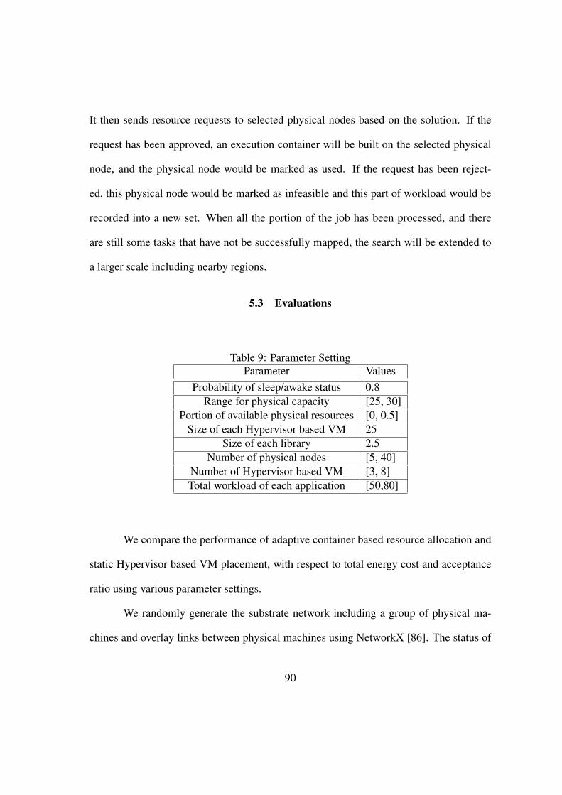
It then sends resource requests to selected physical nodes based on the solution. If the

request has been approved, an execution container will be built on the selected physical

node, and the physical node would be marked as used. If the request has been reject-

ed, this physical node would be marked as infeasible and this part of workload would be

recorded into a new set. When all the portion of the job has been processed, and there

are still some tasks that have not be successfully mapped, the search will be extended to

a larger scale including nearby regions.

5.3 Evaluations



Portion of available physical resources [0, 0.5]Size of each Hypervisor based VM 25

Size of each library 2.5Number of physical nodes [5, 40]

Number of Hypervisor based VM [3, 8]Total workload of each application [50,80]

We compare the performance of adaptive container based resource allocation and

static Hypervisor based VM placement, with respect to total energy cost and acceptance

ratio using various parameter settings.

We randomly generate the substrate network including a group of physical ma-

chines and overlay links between physical machines using NetworkX [86]. The status of

90

each physical node is randomly determined to be awake with an probability of 0.8. Each

physical node is randomly assigned a value between [20, 35] to indicate its maximum

available resource following uniform distribution. To examine the impact of the available

resources on energy consumption, we randomly deduct a portion of available resources

of each physical node to simulate the initial resource usage. The deducted portion is

randomly decided following uniform distribution between [0, θ]. Here we set θ as 0.5.

In addition, we randomly set the type for each physical server. The type of the server

indicates of the differences between available libraries of the physical machines and the

required libraries of the application. When the type of physical server and the type of

the application is n, the necessary libraries that need to be deployed for the container is

n ∗ average size of each library. We assume the average size of each library is 2.5, and

the size of a VM is 25. Parameters used in this chapter is summarized in Table 9.

We first validate our algorithm by comparing it with the optimal solution of VM

placement. The number of physical nodes in this set of evaluations changes from 5 to 40,

while the number of virtual nodes to be embedded is fixed to 5. The total workload of

each application is randomly determined between [50,80].

As presented in Figure [24](a), the VM with fixed requirements on computational

and network may not be able to be embedded into the physical network when the num-

ber of available physical nodes is small, while container based resource allocation could

always properly allocates enough resources for the application. The container based re-

source allocation also outperforms VM placement in total cost as shown in Figure [24](b).

91

10 20 30 40200

300

400

500

Number of Physical Machines

Res

ourc

e P

rovi

sion

ing

Cos

t

VM PlacementEE−CP

10 20 30 400.2

0.4

0.6

0.8

1

Number of Physical Machines

Acc

epta

nce

Rat

io

VM PlacementEE−CP

(a) Total energy cost (b) Acceptance ratio

Figure 24: Comparison for varied number of physical machines

The total cost of provisioning resources for VMs is around 450, while the cost for con-

tainer based resource allocation is around than 250. This cost saving mainly comes from

the memory size savings.

We also examine the impact of the number of VMs in Figure [25](a) and (b).

Here, we vary the number of VMs from 3 to 8. The more VMs to be embedded for the

application, the more redundant memory to be used for building the guest OS, and the

more total cost for the VM embedding. As presented in Figure [25](a), when the number

of VMs increases from 3 to 8, the total cost increases from 376 to 612. However, when to

satisfy the QoS requirement of the same application but with a smaller number of VMs,

each VMs would demand more physical resources. This would increase the difficulties

to embed the VMs, especially when the physical resources are limited. Figure [25](b)

draws when the number of VMs is 3, the acceptance ratio is only 45%. To ensure the

acceptance ratio more than 95%, this work should be spread to at least 5 VMs. Container

92

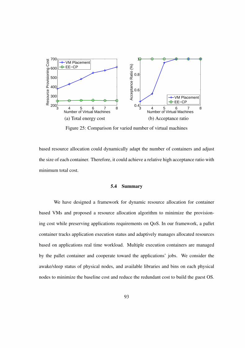
3 4 5 6 7 8200

300

400

500

600

700

Number of Virtual Machines

Res

ourc

e P

rovi

sion

ing

Cos

t

VM PlacementEE−CP

3 4 5 6 7 80.4

0.6

0.8

1

Number of Virtual Machines

Acc

epta

nce

Rat

io (

%)

VM PlacementEE−CP

(a) Total energy cost (b) Acceptance ratio

Figure 25: Comparison for varied number of virtual machines

based resource allocation could dynamically adapt the number of containers and adjust

the size of each container. Therefore, it could achieve a relative high acceptance ratio with

minimum total cost.

5.4 Summary

We have designed a framework for dynamic resource allocation for container

based VMs and proposed a resource allocation algorithm to minimize the provision-

ing cost while preserving applications requirements on QoS. In our framework, a pallet

container tracks application execution status and adaptively manages allocated resources

based on applications real time workload. Multiple execution containers are managed

by the pallet container and cooperate toward the applications’ jobs. We consider the

awake/sleep status of physical nodes, and available libraries and bins on each physical

nodes to minimize the baseline cost and reduce the redundant cost to build the guest OS.

93

Comparisons with static Hypervisor based VM placement shows that the dynamic con-

tainer based VMs has a smaller cost with a higher acceptance ratio.

94

CHAPTER 6

ACHIEVING OPTIMAL CONTENT DELIVERY USING CLOUD STORAGE

While traditional Content Distribution Networks (CDNs), such as Akamai [2]

and Limelight Networks [75], can be expensive for moderate-size content providers, and

building and managing a CDN infrastructure is becoming increasingly difficult [21], the

advent of cloud-based content storage and delivery services provides an economical alter-

native for those content providers. By outsourcing the tasks of maintaining and delivering

a large number of contents to cloud storage providers, content providers, who are also

the cloud users, can significantly cut down their expenditures on building and managing

a storage infrastructure ( [5, 21, 52]). This economic variation of content placement and

delivery attracts a renewed interest on content distribution strategies.

As with traditional CDNs, content providers that use cloud storage are committed

to satisfy content users’ demands within a reasonable response time. In order to reduce

this latency, content providers can disseminate objects on cloud storage servers dispersed

in a network near their users. On the other hand, while emphasizing the content users’ ex-

perience as an overriding concern, content providers also need to consider the expenditure

of cloud storage services that is charged on the occupied storage space and traffic volume

according to cloud storage providers’ polices, such as Amazon Simple Storage Service

(S3) [5] and Google Cloud Storage [52]. While replicating objects on cloud servers can

lower the cost caused by content delivery traffic by cutting down repetitive transmissions,

95

it, however, raises the cost of additional storage space on cloud servers. This opens a new

challenge to design algorithms that could optimize latency as well as cloud storage cost

through replicating contents on proper locations.

Various algorithms have been proposed to optimize content delivery that can be

mainly categorized as Latency-Minimization (LM) algorithms and Traffic-Minimization

(TM) algorithms, according to their optimization aims. The LM algorithms focus on the

optimization of latency; while the TM algorithms concern on the optimization of traffic

consumed by the delivery of contents in backbone networks.

In Chapter 6, we argue that considering the traffic volume together with latency

performance under the constraint on storage cost is crucial for economic and efficient

content delivery service for content providers using cloud services. We have first formu-

lated the joint traffic-latency optimization problem, and proved its NP-completeness. We

then develop an efficient light-weight approximation algorithm, named Traffic-Latency-

Minimization (TLM) algorithm, to solve the optimization problem with theoretical prov-

able upper bound for its performance. To limit the frequency of updates to the origin

server with local changes such as users interests shift, we also extend our TLM algorith-

m in a distributed manner. We provide the theoretical analysis for time complexity and

space complexity of the TLM algorithm, that are O(mnlog(n)), and O(mn) respectively,

where m is the number of proxy servers and n is the number of objects. Unlike most

previous works, our algorithm employs fixable and practical conditions that relax many

assumptions on parameters such as object size, object request probability, the storage ca-

pacity, and the number of requests. Simulation results and experiments show that the

96

performance is near optimal for most of the practical conditions.

The remainder of the chapter is organized as follows. We formulate our network

model and traffic-latency optimization problem, and prove the hardness of the problem in

Section 6.1. We describe our proposed approximation algorithm TLM in both a central-

ized and a distributed manners, as well as its analysis in Section 6.2. The performance

evaluations and comparisons of TLM with prior algorithms are presented in Section 6.3.

The concluding remarks are given in Section 6.4.

6.1 Problem Formulation

Origin serverO

O

Origin serverO

P Proxy serverC

Q P h C ClientQuery Push

PPull

Response

P

P

P

Query Pull (Cooperation)

Query

Response

Response

C C

p

C

Figure 26: Push vs. pull: The origin server pushes some objects to proxy servers. Contentuser queries objects from the proxy server. A proxy server will pull from the origin serveror another cooperative proxy server if it doesn’t have the requested objects.

97

Table 10: Notation UsedNotation Explanation

m The number of proxy serversn The number of objectsi Index of proxy servers, also indicates the service area for

server i, i = 1, 2, . . . ,mci The maximum storage space on proxy server ij Index of objects, j = 1, 2, . . . , ndij The distance from proxy server i to its nearest replica of

object jλi Total number of requests in area ipij Probability that object j will be queried in area isj Size of object jxij Decision variable for pushing object i to proxy server jα Coefficient to balance the weight for latency and data trafficκij Cost for pulling object j to respond the requests for object j

in area i∆mn Total cost for a simple pull strategy with m proxy servers and

n objects, ∆mn =∑m

i=1

∑nj=1 κij

fij Cost saved by pushing object j to proxy server i. fij could bepositive or negative

Fmn Total cost for push-pull strategy with m proxy servers and nobjects, including latency and data traffic cost

As a traditional content distribution network consists of a central origin server and

multiple proxy servers, a content distribution network over a cloud storage is comprised

of an origin server and multiple proxy servers on a cloud network. The proxy servers are

connected with the origin server and/or other proxy servers, as illustrated in Figure 26.

In order to shorten the latency experienced by the final content users, some objects are

replicated on a proxy server, also called a replica, in advance near the users. Moreover,

in order to improve the content users’ experience, proxy servers may cooperate with each

98

other so that they can download objects from others rather than from the origin server.

The proxy servers that are connected by a direct overlay link can communicate with each

other, called neighbors. We assume that the origin server has a sufficient capacity to store

all n objects whose sizes are s1, s2, . . . , sn. However, the storage capacity on each proxy

server i (i = 1, 2, . . . ,m) is limited due to the cost on the cloud storage space, which

makes it impossible to replicate all n objects on each proxy server i, (i = 1, 2, . . . ,m).

Thus, we need a salient distribution strategy to decide if it is better to replicate object j

on proxy server i in advance. Notations used in Sections 6.1 and 6.2 are summarized in

Table 10.

6.1.1 The Push-Pull Model

In our model, each proxy server takes charge of one area of service, which can

be assigned according to geographic locations or domains as in [123]. Content users in

area i will directly request and download objects from the proxy server i. For simplicity

of our discussion, we denote a proxy as if there is only one proxy server per one area. In

practice, an origin server may be a server farm, and more than one proxy server may be in

charge of one area. In such a case, the sum of proxy servers’ storage space for area i can

be used as ci. Notice that cloud storage requires multiple replication based on predefined

replication factor. The available storage space will be the actual storage size divided by

the replication factor. Here, we assume that the same replication factor will be applied for

all the contents, and use ci as the available storage space for distinct contents. The issue of

necessary number of proxy servers in an area has been studied in [112,113]. Additionally,

99

servers in a data center are typically clustered and situated in a close location, resulting in

little difference in delay to a user from any of the servers in a farm.

In satisfying content users’ requests, two typical schemes can be considered for

content distribution, a push-based scheme and a pull-based scheme. In a push-based

scheme, objects are replicated into proxy servers prior to requests until a proxy server’s

storage limitation is reached. This distribution procedure is referred to as a push. When

requests arise for those pushed objects, a proxy server will directly serve the content users

without involving other cloud servers. On the other hand, no object is replicated into the

proxy servers in advance under a pull-based scheme. When proxy servers receive queries

for the un-pushed objects, they will forward the query and download the requested objects

from the nearest source that could be either the origin server or another cooperative proxy

server. This procedure is specified as a pull. By disseminating objects in advance, a push-

based scheme shortens the retrieval latency of object j; while a pull-based scheme reduces

traffic volume by eliminating object downloads that would never be requested. In order to

optimize both latency cost and traffic cost, we consider a content delivery scheme that is

the combination of a push-based scheme and a pull-based scheme. This push-pull scheme

is expected to properly determine which objects should be pushed and which should be

pulled, so that both the push-based scheme and pull-based scheme are used to their best

advantages. We formulate the push-pull scheme in Section 6.1.2 as an optimization prob-

lem and solve it with our Traffic-Latency-Minimization (TLM) algorithm in Section 6.2.

100

6.1.2 The Push-Pull Optimization Problem

We point out that we focus on the performance within a distribution cloud network

and do not compute the latency and traffic costs between a proxy server and the final con-

tent users. In fact, those costs will not be impacted by the content distribution strategies,

since each content user is directly served by a fixed proxy server according to the users’

location. Therefore, our problem is to minimize the total cost, that includes the latency

cost and the traffic cost between cloud servers, to satisfy all the requests from content

users.

From the content providers’ point of view, the overriding concerning is to ensure

the content users’ experience; however, it is also significant to reduce costs for maintain-

ing and delivering contents. Therefore, the costs for content delivery over cloud storage

should include latency cost, which is related to the experience of final content users, and

the traffic cost that is the main characteristic to estimate the expenditure for cloud service.

The latency in area i to obtain object j corresponds with the distance dij between

proxy server i and its nearest replica of j. dij could be either spacial, such as the number

of hops as used in [67, 71] or temporal, such as the average round trip time that can be

predicted with the methods proposed in [80, 105]. The latency from a proxy server to

different users may vary depending on a user’s access network and the path. However, in

this chapter, we focus on the latency from the location of a requested objects to the proxy

server that directly serve a final user, and omit the latency from this proxy server to the

final user. The related discussion about latency from proxy servers to final users can be

found in [65].

101

When a request is raised for object j in area i, if j has already been pushed into

the proxy server i, proxy server i can respond immediately without involving any extra

latency. However, if object j has not been replicated on proxy server i in advance, proxy

server i needs to pull object j from either the origin server or another cooperative proxy

server that results in an additional latency cost dij for each request for object j in area i.

Assume the total number of requests for object j in area i is the product of λi, which is

the total number of requests in area i, and pij , which is the probability that object j will

be queried in area i, then the expectation of the total latency cost in area i is dijpijλi for

un-pushed object j. We highlight that the request patterns are heterogeneous depending

on the area, which means we introduce various λi and pij in a different service area i. It

is more practical than the assumption of a fixed request pattern used in previous studies

such as [10, 67].

On the other hand, sj that is the size of object j is utilized to estimate the traffic

cost. Furthermore, if object j has been pushed to the proxy servers, the amount of sj is

appended to the traffic cost for each replica of object j. Otherwise, the amount of sj is

added for each query for object j.

We use a matrix X to present an allocation of replicas with the push-pull strategy,

and each element xij in X indicates whether object j should be pushed to a proxy server

i or not.

xij =

{1, Object j is pushed on proxy server i

0, Object j is not pushed on proxy server i(6.1)

Now, the expectation of accumulated latency in a cloud storage networks using

102

the push-pull strategy can be represented as:

m∑i=1

n∑j=1

(1− xij)dijλipij (6.2)

and the total traffic volume for this network can be formulated as:

m∑i=1

n∑j=1

(xijsj + (1− xij)sjλipij) (6.3)

As we consider the costs of both latency and traffic, we use a coefficient α to

balance the influence of latency and traffic costs to satisfy various application and per-

formance requirements. Then, our objective is to minimize this weighted total cost of

latency and traffic for this network when using the push-pull strategy under the storage

constraints.

m∑i=1

n∑j=1

(1− xij)dijλipij + α

m∑i=1

n∑j=1

(xijsj + (1− xij)sjλipij) (6.4)

subject to storage constraints:

n∑j=1

xijsj ≤ ci, i = 1, 2, . . . ,m (6.5)

To solve this optimization problem, we simplify Eq. (6.4) and obtain

min(m∑i=1

n∑j=1

(dijλipij + αsjλipij − xij(dijλipij + αsjλipij − αsj))) (6.6)

Eq. (6.6) can be further derived as:

minm∑i=1

n∑j=1

(κij − xijfij) (6.7)

where κij = dijλipij + αsjλipij and fij = dijλipij + αsjλipij − αsj . Note that κij

denotes the weighted total cost for un-pushed object j in area i, and fij represents the

relative saved cost by pushing object j to proxy server i.

103

When λi that is the number of requests in area i, popularity pij for object j in

area i, distance dij from the nearest replica of object j to the proxy i and size sj for

object j are determined, the weighted total cost of the simple pull strategy by which no

object is replicated on the proxy server in advance, will not be impacted by the replica

allocation. Therefore we denote ∆mn =∑m

i=1

∑nj=1 κij as the weighted total cost for a

simple pull cloud storage network with m proxy servers and n objects when every request

is responded to by pulling. Then, the optimization problem described in Eq. (6.4) is

equivalent to

maxm∑i=1

n∑j=1

(xijfij) (6.8)

subject to storage constraints:n∑

j=1

xijsj ≤ ci, i = 1, 2, . . . ,m (6.9)

where fij is utilized to signify the cost saving by pushing object j to proxy server i. In

addition, fij could be positive or negative. fij > 0 means that pushing object j to proxy

server i can reduce the weighted total cost, while fij < 0 suggests that pushing object j

to proxy server i will increase the cost. When fij = 0, pushing object j to proxy server i

cannot save the weighted total cost, but takes up additional storage space on proxy server

i that results in increased cloud storage cost. Thus, we only consider the object j with a

positive fij as a candidate to be pushed on proxy server j.

Consider the special cases of Eq. (6.4). When α is set to 0, it is reduced to a

simple latency minimization problem when α is set to 0. It is reduced to a simple traffic

minimization problem, when α is set to a large number, such as 100 or 1000, assuming

that latency cost and traffic cost are with the same order of magnitude.

104

6.1.3 Hardness of the Problem

As we presented in Section 6.1.2, our aim is to optimize the weighted total cost

of latency and traffic under the storage constraints by solving the optimization problem

Eq. (6.4) subject to Eq. (6.5), named the push-pull optimization problem. As we illustrated

in Section 6.1.2, Eq. (6.4) is equivalent to Eq. (6.8) that we named the push-pull equivalent

problem. We demonstrate the NP-completeness of the push-pull equivalent problem by

using the well-know Knapsack problem and considering a special case of the push-pull

equivalent problem, so that we prove the hardness of the push-pull optimization problem.

Before we present the NP-completeness of the push-pull equivalent problem, we first re-

state this push-pull equivalent problem as well as the push-pull optimization problem and

the Knapsack problem.

Push-pull optimization problem: Given a set of n objects with varying sizes s1, s2, . . . , sn,

varying locations and the probability that they will be queried, the problem is to figure out

whether there is any allocation X , with which the weighted total cost of a push-pull s-

trategy over cloud storage is less than a constant value F , and the total size of the objects

pushed to proxy server i is smaller than ci, i = 1, 2, . . . ,m as in Eq. (6.5) or not.

Push-pull equivalent problem: Given a set of n objects with varying sizes s1, s2, . . . , sn,

varying locations and the probability that they will be queried, the problem is to figure out

if there is a group of object j, by pushing which to certain proxy server i, the amount of

the weighted total cost of a simple pull network over cloud storage can be saved more

than a constant value F −∆mn, and the total size of objects pushed to the proxy server i

is smaller than ci, i = 1, 2, . . . ,m as in Eq. (6.9), where ∆mn is the weighted total cost

105

of the simple pull network with m proxy servers and n objects.

Knapsack problem: Assume a set of n items with varying weights w1, w2, . . . , wn,

and values v1, v2, . . . , vn. The problem is to determine whether or not there is any subset

of these n items so that the total weight of this subset is no more than a given limit W

while the total value is larger than V .

We consider a special case of the push-pull equivalent problem, where we have

only one proxy server 1 with the storage capacity c1. We need to determine the group of

objects to be pushed on the proxy server 1 so that the weighted total cost can be saved

more than a constant F − ∆mn. Because the original push-pull problem equivalent is

more complex than this special case, if the special case is proved to be NP-complete,

the original problem is NP-complete, and the original push-pull optimization problem is

NP-complete as well.

First, it is easy to prove that the special case of the push-pull equivalent problem

belongs to NP. Any object allocation can be examined if it is a feasible solution that the

weighted total cost is saved more than F − ∆mn and it meets the storage constraint in

polynomial time. Next, we prove that the Knapsack problem, that is a well known NP-

complete problem, can be reduced to the special case of the push-pull equivalent problem

in polynomial time. By letting weight wj correspond to size sj of object j and value

vj correspond to the cost saving f1j of pushing object j to proxy server 1, this means

wj = sj and vj = f1j . Let the weight limitation W correspond to storage constraint

c1 while the value limitation V corresponds to the weighted total cost saved by pushing

object (F −∆mn), where W = c1 and V = (F −∆mn), the Knapsack problem is reduced

106

to our push-pull problem. Therefore, if the solution of the Knapsack problem is known,

the corresponding set of objects is a solution of the push-pull equivalent problem as well

as the solution for the push-pull optimization problem.

6.2 Approximation Algorithm

In this section, we develop an approximation algorithm toward an optimal solu-

tion of the push-pull optimization problem, and then we establish a theoretical efficiency

bound and produce a performance analysis for this approximation algorithm.

As we demonstrated in Section 6.1.2, the weighted total cost of a push-pull net-

work over cloud storage is equal to the weighted total cost of a simple pull network sub-

tracting the cost saved by pushing a group of objects. Thus, we can solve the push-pull

optimization problem by determining a group of objects, so that the weight total cost

saved can be maximized by pushing them to proxy servers in advance.

One naıve heuristic algorithm could be choosing the objects in the decreasing

order of fij , which is the amount of saved weighted total cost for pushing object j to

proxy server i. However, this does not best utilize the storage toward the maximum saved

weighted total cost in Eq. (6.8), or in other words, the minimum weighted total cost in

Eq. (6.4).

Instead, we design an approximation algorithm that selects objects that can max-

imize saving the weighted total cost while occupying a small storage space. We first

compute

rij = fij/sj (6.10)

107

Storage capacity : c1 = 8

Object 1: s1 = 3, fi1= 4(a) Object 2: s2 = 3, fi2= 3

Object 3: s3 = 8, fi3 = 7.5(b) j 3 , i3(b)

Figure 27: ri1 = 1.33; ri2 = 1; ri3 = 0.94. Pushing object 1 and 2 with the lowest ratiori1 and ri2(case (a)) is worse than pushing object 3 (case (b)).

, which is the ratio of the push-pull cost saved for pushing object j to proxy server i and

the size of object j. Then, the objects with the highest ratio will be pushed to proxy server

i while the space is allowed within the storage constraint as in Eq. (6.5).

We observe that using only the ratio rij to determine whether pushing object j to

proxy server i may not be a good solution in some scenarios, as illustrated in Figure 27.

In this occasion, a proxy server i has an available storage amount of ci = 8, and there

are three objects, (object 1,2, and 3) with decreased rij (ri1 = 1.33, ri2 = 1, ri3 = 0.94).

Proxy server i cannot replicate all the three objects due to the storage limitation. There-

fore, the problem turns into the selection of objects to be replicated. Suppose the sizes

and the push-pull cost differences for objects 1, 2, and 3 are (s1 = 3, fi1 = 4), (s2 =

3, fi2 = 3), and (s3 = 8, fi3 = 7.5), respectively. If we push objects according to the

ratio of push-pull cost differences to the size, object 1 and object 2 will be replicated to

proxy server i in advance. However, under this case, 2 units of spare room in the cache

108

will be left, which is not enough for other objects to be replicated in this proxy server.

Therefore, the weighted total cost is ∆mn − 7 according to Eq. (6.8) and Eq. (6.10),

where ∆mn =∑3

j=1 κij . On the other hand, if object 3 is chosen to be pushed, all the

space has been efficiently used, and the weighted total cost is ∆mn − 7.5 that is smaller

than pushing object 1 and object 2.

This problem can be addressed by comparing the weighted total cost of objects

with the highest rij that can be pushed, subject to a storage constraint with the cost of

the first object that cannot be pushed. By adding this comparison, the weighted total

cost of the modified algorithm will be bounded less than ∆mn − 12

∑j∈OptSet fij , while

the optimal total cost is ∆mn −∑

j∈OptSet fij . Based on this observation, we propose an

approximation algorithm, named the Traffic-Latency-Minimization (TLM) algorithm as

depicted in Algorithm 6.

As described in Algorithm 6, we first calculate fij , the saved weighted cost by

pushing object j to proxy server i and rij , the ratio of fij and the object size sj for each

object j. We further compute the weighted total cost for a simple pull network over

cloud storage with these m proxy servers and n objects. Then, we sort the objects in

descending order according to their rij and push the objects with positive rij until the

storage limitation of proxy server j has been reached. When there is not enough space for

object j in proxy server i, we compare the saved weighted total cost of all already pushed

objects with the possible saved cost of pushing object j, if pushing object j can save more,

we remove pushed objects on proxy server i until there is enough space to replicate object

j; otherwise, we do nothing and move to the next object.

109

Algorithm 6 TLM approximation algorithm - runs on origin server

for every proxy server i ∈ {1, 2, . . . ,m}Calculate fij and rij for each object j ∈ {1, 2, . . . , n};Sort rij in descending order and record corresponding indices in arrayh;Calculate total cost of system TotalCost = TotalCost+

∑nj=1 κij;

Keep a record of the weighted total cost for a simple pull system∆mn = ∆mn +

∑nj=1 κij;

for index ∈ {1, 2, . . . , n}j = h[index];if (rij > 0 AND sj ≤ available storage on i)

Put j into PushSeti;TotalCost = TotalCost− fij;

else if (rij > 0 AND sj > available storage on i)if (∆mn − fij < TotalCost AND sj ≤ ci)

Keep removing the last element in PushSeti till thereis enough room for j;Update TotalCost;Put j into PushSeti;

end ifelse if rij ≤ 0

Break;end if

end forend for

Next, we prove the bounded quality of our approximation algorithm.

Theorem 1. The upper bound of the TLM approximation algorithm is ∆mn−12

∑j∈OptSet fij ,

if the optimal total cost is ∆mn −∑

j∈OptSet fij .

Proof. Suppose a list of objects j, j = 1, 2, . . . , n are sorted in a descending order ac-

cording to rij the ratio of fij , saved weighted total costs if pushing object j on proxy

server i and object size sj . In the list, object 1 has the largest ratio ri1, which means

110

Object 1 Object 2 Object (L!1)…(a)

Object L(b)

Figure 28: In TLM, either object 1, . . . , L − 1, (L > 1) or object L can be pushed to aproxy server.

Object L

Obj 1 Obj 2 Obj (L 1)Object 1 Object 2 Object (L!1)…

Figure 29: The upper bound of optimal solution

pushing object 1 to proxy server i reduces the most cost per bit up to s1 bits; while object

n has the smallest ratio rin, which indicates pushing object n reduces the least of the cost

per bit when taking up to sn bits space. Without loss of generality, we only consider the

objects with ratios rij larger than 0, which means the optimal solution is to push all of

these objects in order to minimize total weighted cost of the system. However, the total

size of those objects can be larger than the storage space in the proxy server. Therefore,

we push objects one by one according to the sorted order until the storage constraint of

111

proxy server i is reached.

As is shown in figure 28, we assume that object L is the first object that cannot be

pushed into proxy server i subjected to a storage constraint of i. If objects can be divided

into pieces, pushing {object 1, object 2,. . . , object (L−1)} and a fraction of object L will

provide the smallest total cost

∆mn −L−1∑j=1

fij −ci −

∑L−1j=1 sj

sLfiL (6.11)

which is described in Figure 29. However, objects cannot be partitioned in our push-

pull optimization problem. Thus, the optimum result of our optimization problem cannot

surpass that of the fractional optimization problem. Suppose OptSet is the object set of

the optimal solution for non-fractional optimization problem, the weighted total cost of

this set is

∆mn −∑

j∈OptSet

fij (6.12)

that will not be smaller than the cost in Eq. (6.11).

According to our algorithm, if∑L−1

j=1 fij ≥ fiL, object 1, object 2,. . . , object (L−

1) will be pushed into the proxy server i; otherwise, object L will be pushed into the proxy

server i. Then, we have either∑L−1

j=1 fij ≥ 12

∑j∈OptSet fij or fiL ≥ ci−

∑L−1j=1 sj

sLfiL ≥

12

∑j∈OptSet fij Therefore, the weighted total cost of our algorithm is

min{∆mn −L−1∑j=1

fij,∆mn − fiL} (6.13)

from which the upper bound of our algorithm can be derived as

∆mn −1

2

∑j∈OptSet

fij (6.14)

112

We now discuss the time and space complexity of the proposed algorithm. The

algorithm computes PushSeti for each proxy server i ∈ 1, 2, . . . ,m. In each iteration,

ratios rij are sorted in O(nlog(n)) time. Therefore, the total time complexity of the

approximation algorithm is O(mnlog(n)).

On the other hand, O(n) storage space is needed in order to sort the ratios and

record the PushSeti for each proxy server i ∈ 1, 2, . . . ,m. However, because iterations

are executed serially, the O(n) storage space for sorting can be reclaimed in each iteration.

Meanwhile, considering m proxy servers, the space required for m PushSeti is O(mn).

Thus, the total space complexity of the proposed approximation algorithm is O(mn).

Note that the approximation algorithm can be further improved with the upper bound as

∆mn − (1 − ε)∑

j∈OptSet fij , where ε > 0, but with an increased time complexity of

O(mnlog(1ε) + m 1

ε4), and an increased space complexity of O(mn + m 1

ε3) as proved

in [72].

Finally, driven by the requirement of offloading the work of origin server and

backbone networks, the proposed approximation algorithm can be implemented in a dis-

tributed manner as depicted in Algorithm 7. The Distributed Traffic-Latency-Minimization

(DTLM) algorithm is running on each proxy server to enable proxy servers to dynamical-

ly adjust the distribution of replica so that economically and efficiently server the content

users’ requirements without burdening the origin server.

As presented in Algorithm 7, each proxy server i first calculates the PushSeti

that includes the objects to be pushed on proxy server i, based on the assumption that the

113

Algorithm 7 DTLM approximation algorithm - runs on each proxy server

Initialize the distance dij for each object j as the distance from originserver to local;Initialize the location of each object j as origin server;Calculate the fij and rij for each object j;Sort rij in descending order and record corresponding indices in array h;Calculate the PushSeti according to rij and current dij;Update the location for objects in PushSeti as local;Inform cooperative-proxy server about current PushSeti;While (receive PushSeti′ from cooperative proxy server i′)

For each objects k in received cooperate-proxy server’s PushSeti′;If distance from proxy server i′ to local is nearer than dij;

update dij as the distance from proxy server i′ to local;record the location of object k as proxy server i′;

End ifEnd forFor each objects j

If (Location is proxy server i′) AND (Not in PushSet′i)Update the distance dij as the distance from origin serverto local;Update the location of object j as origin server;

End ifEnd forRecalculate the fij and rij for each object j;Recalculate the PushSeti according to updated rij and current dij;Inform cooperate-proxy server updated PushSeti;

End while

114

nearest replica is on the origin server. After that, proxy server i informs its cooperative

proxy servers about PushSeti and meanwhile notified by its cooperative proxy servers

about their PushSet′i. Then proxy server i may update the distance dij between the n-

earest replica of object j and proxy server i if j is in PushSet′i, and recomputes a new

PushSeti by using updated distance dij . By continuously exchanging the PushSeti with

the cooperative proxy server and recompute the PushSeti based on PushSet′i received

from cooperative proxy server, proxy server i can gradually approach the optimal solution

that has a minimum weighted total cost of the push-pull network. The space complexity

of DTLM is O(n) on each proxy server. Limited rounds of control messages are ex-

changed only among neighbors with their lists of objects. Upon receiving messages from

neighbors, O(nlog(n)) of the time complexity is spent.

6.3 Evaluations

In this section, we conduct extensive performance evaluations of our proposed ap-

proximation algorithms, TLM, and its distributed version, DTLM, using both simulations

with parameters from practices and experiments on a real network.

6.3.1 Simulations

We first describe the parameters used for simulations. In our simulation, a proxy

server i is randomly endowed with a different storage capacity ci, the mean of which is

set to 25% of the total object size to obtain an ideal CDN utility and hit ratio [103]. Also,

each object is associated with a size sj that is retrieved from real .avi files, which range

from 1.28 MB to 41.8 GB. Each object has its probability of being requested in each area,

115

Table 11: Parameter Setting for SimulationsParameter Values

m Number of proxy servers, m = 10ci ∼ normal distribution N(0.25 ∗ jGB, 1GB2)n Varies in the range of [100, 200, . . . , 1000]sj Sizes of real media files, range in [1.28MB 41.800GB]pij ∼ Zipf distribution Z(1, n)α 0.5dij ∼ normal distribution N(10 hops, 5 hops2). 15 ms per hop.λi ∼ normal distribution N(200 requests, 100 requests2)

200 400 600 800 10000

5

10

15

Number of Objects

Tot

al C

ost (

105 )

TLMDTLMTMLM

200 400 600 800 10000

1

2

3

Number of Objects

Tra

ffic

Vol

ume

(106 M

b) TLMDTLMTMLM

200 400 600 800 10000

1

2

3

Number of Objects

Late

ncy

(105 m

s)

TLMDTLMTMLM

(a) Total cost (b) Traffic overhead (c) Latency overhead

Figure 30: Comparison for varied number of objects (simulation with real object sizes)

following a Zipf distribution. In particular, the probability of object j to be demanded

in area i is 1/kijHn,1

.1 The cost coefficient α in (6.4) is set to balance the traffic volume and

latency requirements. In Figures 30 and 31, we set α as 0.5 so that the requirements of

traffic volume and latency are of equal weights. We then show how α can be used for

different requirements in Figure 32. The parameters used in this simulation are described

in Table 11.1k is the rank of the decreasing probability list of objects, out of [1, n], where n is the number of objects.

Hn,1 is the nth harmonic number. Hn,1 = 1 + 1/2 + 1/3 + ...+ 1/n.

116

We compare the performance of the proposed algorithm with other existing algo-

rithms that minimize traffic volume – referred to as the Traffic-Minimization (TM) algo-

rithm – as in [18], and that minimize latency – referred to as the Latency-Minimization

(LM) algorithm – as in [67], respectively. In [18], the objects are replaced dynamically

with the highest global utility in the proxy servers that can be referred to as a pull-based

scheme; meanwhile, in a push-based scheme such as [67], the objects are replicated ac-

cording to their popularity and transmission distance.

Figures 30 (a), (b) and (c) compare the total cost of the traffic overhead and the

latency overhead of three algorithms, respectively, as the number of objects increases. We

have varied the total number of objects ranging from 100 to 1000 as in [65, 67, 74, 107].

In Figure 30 (a), we observe the total cost of the proposed algorithm, TLM, and

the compared algorithms, BM and LM. It shows that the proposed TLM and DTLM uses

the lowest cost, and outperforms BM and LM algorithms that consider traffic volume

or latency individually, especially as the demand increases. When we investigate the

individual performance of traffic and latency, the proposed TLM and DTLM algorithm

achieves a good tradeoff between traffic volume and latency, and is closer to the lowest,

as shown in Figures 30 (b) and (c). We observe that, TLM performs slightly better than

DTLM. That is because the origin server has the complete knowledge of the placements of

each object’s replica; while proxy servers in DTLM only have limited knowledge shared

from neighbors. On the other hand, there is no significant improvement of TLM, since

network issues such as packet loss and queueing delay are not captured in the simulations.

Therefore, we further examine the performance of TLM and DTLM in a real test platform,

117

0 500 10006

8

10

12

14

16

Standard Deviation

Tot

al C

ost (

105 )

TLMDTLMTMLM

0 500 10001

1.5

2

2.5

3

Standard Deviation

Tra

ffic

Vol

ume

(106 M

b)

TLMDTLMTMLM

0 500 1000

0.5

1

1.5

Standard Deviation

Late

ncy

(105 m

s) TLMDTLMTMLM


Figure 31: Comparison for varied standard deviation of object sizes (simulation withsynthetic object sizes)

0 0.05 0.1 0.5 1 10 1000

1

2

3

α

Tot

al C

ost (

108 )

TLMDTLMTMLM

0 0.05 0.1 0.5 1 10 1000

1

2

3

α

Tra

ffic

Vol

ume

(106 M

b)

TLMDTLMTMLM

0 0.05 0.1 0.5 1 10 1000

0.5

1

1.5

2

α

Late

ncy

(105 m

s)

TLMDTLMTMLM


Figure 32: Comparison for varied balance parameter α (simulation with real object sizes)

Planetlab.

We further investigate the impact of the variance of object size in Figures 31 (a),

(b), and (c). Object sizes in this group of experiments are randomly selected from a normal

distribution N(1 GB, V a MB2), where V a varies from [0, 1000]. As observed in Figure

31 (c), when the standard deviation increases, latency cost by LM steadily increases. This

poses less impact on TLM and DTLM.

In addition, the impact of balance parameter α is presented in Figures 32 (a), (b)

118

Table 12: Parameter Setting for Planetlab ExperimentsParameter Values

m Number of proxy servers, m = 10ci ∼ normal distribution N(0.25 ∗ jGB, 1GB2)n Varies in the range of (100, 200, . . . , 1000)sj Size of real media files, range in [1.28MB 41.800GB]pij ∼ Zipf distribution Z(1, n)α 0.05dij Real distances between Planetlab sitesλi ∼ normal distribution N(200 requests, 100 requests2)

and (c). As exhibited in Figures 32 (b) and (c), when α is set to 0, TLM and DTLM

are reduced to simply minimize latency while when α is approaching infinite, TLM and

DTLM will simply minimize traffic volume. However, the weighted total costs of TLM

and DTLM are always the least compared with BM and LM.

6.3.2 Experiments

In order to validate the efficiency and effectiveness under a more realistic environ-

ment, we also evaluate our algorithm on Planetlab testbed [90]. Furthermore, for realistic

purpose, we employ real object sizes instead of randomly assigning them as we do in the

simulation portion. Object sizes are obtained from a search engine by searching media

objects. As in simulations, the experiments are implemented with 1 origin server and 10

proxy servers, and the network topology is presented in Figure 33. The distance between

servers are derived from real RTT times between these 11 Planetlab sites. The other pa-

rameter settings, such as proxy servers’ storage ability, popularity and request number in

each area are the same with those in the simulations.

119

Figure 33: Locations for the origin server and proxy servers: the mark in the circle indi-cates the location for the origin server; and the remain sites are all proxy servers. Eachproxy server is connected to origin server and its cooperative proxy servers. Proxy serversmay pull objects from the origin server or a closer proxy server.

As in the evaluation with simulations, we have studied the total cost, the traffic

overhead, and the latency overhead of three algorithms in Figures 34 (a), (b) and (c), re-

spectively, as the number of objects increases from 100 to 1000. The balanced coefficient

α is set to 0.05 to enforce the traffic volume and latency work in the same order. We

summarize the parameters in experiments in Table 12.

As shown in Figure 34 (a), both TLM and DTLM outperform LM and BM algo-

rithms in the total cost that considers both traffic volume and latency. DTLM performs

a little worse than TLM, since it may not find the most proper replica location for ev-

ery object. Furthermore, as depicted in Figures 34 (b) and (c), we find that our TLM

and DTLM algorithms can find a good tradeoff between latency and traffic volume con-

sumption, which conforms to the observations we have made from the simulations. The

differences in the values of total cost, traffic, and latency consumption in simulation and

120

200 400 600 800 10000

5

10

15

Number of Objects

Tot

al C

ost (

104 )

TLMDTLMTMLM

200 400 600 800 10000

1

2

3

Number of Objects

Tra

ffic

Vol

ume

(106 M

b) TLMDTLMTMLM

200 400 600 800 10000

5

10

Number of Objects

Late

ncy

(104 m

s)

TLMDTLMTMLM


Figure 34: Comparison for varied number of objects (Planetlab experiments with realobject sizes)

0 500 1000

1

1.5

2

2.5

Standard Deviation

Tot

al C

ost (

105 )

TLMDTLMTMLM

0 500 10001

2

3

4

5

Standard Deviation

Tra

ffic

Vol

ume

(106 M

b) TLMDTLMTMLM

0 500 1000

2

4

6

8

10

12

Standard Deviation

Late

ncy

(104 m

s)

TLMDTLMTMLM


Figure 35: Comparison for varied standard deviation of object sizes (Planetlab experi-ments with synthetic object sizes)

experiments come from the object sizes and distance settings.

The impact of size variance is also examined on Planetlab as presented in Figures

35 (a), (b) and (c). The number of objects is 1000 as used in [65, 67, 74, 107], and the

storage limitation for each proxy server is 250 GB. The size of objects follows normal

distribution with mean 1 GB, and standard deviation varies from 0 to 1 GB2. As shown

in Figure 35 (c), as standard deviation varies, the latency consumed by the LM algorithm

increases, while the latency of the other three algorithms stays stable.

121

0 0.05 0.1 0.5 1 10 1000

0.5

1

1.5

2

2.5

α

Tot

al C

ost (

108 )

TLMDTLMTMLM

0 0.05 0.1 0.5 1 10 100

1

2

3

4

α

Tra

ffic

Vol

ume

(106 M

b) TLMDTLMTMLM

0 0.05 0.1 0.5 1 10 1000

0.5

1

α

Late

ncy

(105 m

s)

TLMDTLMTMLM


Figure 36: Comparison for varied balance parameter α (Planetlab experiments with realobject sizes)

We further investigate the impact of balance parameter α in Figures 36 (a), (b)

and (c). As presented in Figures 36 (a), (b) and (c), α can be used to balance the impact

of latency and traffic volume requirements. Especially, TLM and DTLM can be reduced

to simply minimize latency or traffic volume by setting α to 0 or a very large value (e.g.

100), respectively.

6.4 Summary

We have studied the problem of content placements that determines which objects

should be pushed to which proxy servers and which should be pulled on demand for an

optimal content delivery over cloud storage. To the best of our knowledge, our work is

the first to consider both bandwidth usage in the network and latency for the optimization

of content delivery using cloud storage services. We have modeled and formulated this

122

push-pull content delivery problem, and proved that it is NP-complete using the Knap-

sack problem. We have developed an approximation algorithm named Traffic-Latency-

Minimization (TLM) for our push-pull optimization problem. Theoretical analysis indi-

cates that the upper bound of the TLM algorithm is ∆mn − 12

∑j∈OptSet fij comparing

that the optimal solution can achieve ∆mn −∑

j∈OptSet fij , where ∆mn is the weighted

total cost for a simple pull strategy and fij denotes the saved cost by pushing object j to

proxy server i. The time complexity of our TLM algorithm is Θ(mnlog(n)), while the

space complexity is O(mn). In our model, we have made system parameters such as the

storage capacity, the number of requests, object request probability, and object size to be

dynamic rather than constant. We have further implemented a distributed algorithm for

our TLM algorithm named DTLM and compared our TLM and DTLM algorithms with

other existing algorithms with simulations and experiments. We have also shown that

our approximation algorithm, both in a centralized and a distributed manners outperforms

them, reaching near the minimum cost of both latency and bandwidth.

Several related challenges need to be addressed before deploying into a real con-

tent distribution system. Relevant future work would include developing an accurate on-

the-fly estimation scheme for the demands, the methods for short and long-term optimal

cache dimensioning and placements, and content delivery based on different Service Lev-

el Agreements.

123

CHAPTER 7

CONCLUSIONS AND FUTURE WORK

This dissertation focus on energy efficient resource allocation for virtual network

service in cloud data centers. New models are proposed and studied to minimize the

cost in resource allocation for virtual networks, virtual machines and cloud storage ser-

vices while persevering QoS requirements of network services. We consider practical

constraints and demands, such as time evolving workload of virtual services and avail-

able physical resources, practical DC topologies. In addition,green physical nodes that

enables sleep/awake mode are employed to improve energy efficiency in data centers.

For the energy efficient virtual network embedding, we plan possible future migra-

tion in advance, and minimize the total energy consumption including both operation cost

and potential future migration cost. An efficient and practical virtual network embedding

algorithm (TMAE-VNE) and an Ant Colony Optimization based memory efficiency al-

gorithm have been developed to determine the initial embedding and future migration for

a virtual networks considering its predictable demands. Extensive comparisons with ex-

isting VNE algorithms validated the improvements of the proposed algorithms in energy

saving and acceptance ratio under various scenarios.

In addition, container based virtual machine embedding and resource allocation

attracts more attentions as its light weight and efficiency. Driven by the advantages of

124

container based VM, we proposed a novel framework to provision resources for virtu-

al network services utilizing container based VM. In our framework, we separated the

resource management and job execution for the network services into two kinds of con-

tainers named as pallet container and execution container. We further designed a cost

efficiency resource allocation model and corresponding algorithm to solve this problem.

Compared with static Hypervisor based VM placement, evaluations validated that con-

tainer based resource allocation improves the acceptance ratio and cost efficiency.

Finally, we studied content placement problem with the optimization goal to mini-

mize the bandwidth usage in the network and latency experienced by final users. We mod-

eled the push-pull content delivery problem and proved its hardness. Later an approximate

algorithm has been designed and developed with guaranteed bound. We implemented the

algorithm in a distributed manner as well as a centralized manner and compared them

with existing algorithms through simulations and experiments on planetlab.

Resource allocation is one of the most essential problem in cloud computing. As

the development of cloud computing and the advent of new techniques, such as the uti-

lization of fiber optic in data centers, multi-regional electricity markets, edge cloud and

mobile cloud, new challenges and new opportunities would be brought to resource alloca-

tion problem. These new scenarios will be further explored and taken into consideration

in the future.

125

REFERENCE LIST

[1] 15% Growth Forecast for North America Colocation Market 2014.

http://www.datacenterdynamics.com/focus/archive/2014/01/15-growth-forecast-

north-america-colocation-market-2014-0.

[2] Akamai. http://www.akamai.com/.

[3] Al-Fares, M., Loukissas, A., and Vahdat, A. A scalable, commodity data center

network architecture. In Proceedings of the ACM SIGCOMM 2008 conference on

Data communication (New York, NY, USA, 2008), SIGCOMM ’08, ACM, pp. 63–

74.

[4] Almeida, J. M., Eager, D. L., Vernon, M. K., and Wright, S. J. Minimizing delivery

cost in scalable streaming content distribution systems. IEEE Trans. Multimedia 6,

2 (2004), 356–365.

[5] Amazon Simple Storage Service (Amazon S3). http://aws.amazon.com/s3/.

[6] Amokrane, A., Zhani, M., Langar, R., Boutaba, R., and Pujolle, G. Greenhead: Vir-

tual Data Center Embedding across Distributed Infrastructures. Cloud Computing,

IEEE Transactions on 1, 1 (Jan 2013), 36–49.

[7] Andersen, D. G. Theoretical approaches to node assignment. Computer Science

Department (2002), 86.

126

[8] Arlitt, M. Characterizing web user sessions. ACM SIGMETRICS Performance

Evaluation Review 28, 2 (2000), 50–63.

[9] at Scale, G. G. C. E. https://static.googleusercontent.com/media/www.google.com/en//green/pdfs/google-

green-computing.pdf.

[10] Baev, I., Rajaraman, R., and Swamy, C. Approximation algorithms for data place-

ment problems. SIAM J. Computing 38, 4 (2008), 1411–1429.

[11] Baev, I. D., and Rajaraman, R. Approximation al-

gorithms for data placement in arbitrary networks.

Proc. 12th Annu. ACM-SIAM Symp. Discrete algorithms (SODA) (2001),

661–670.

[12] Barham, P., Dragovic, B., Fraser, K., Hand, S., Harris, T., Ho, A., Neugebauer, R.,

Pratt, I., and Warfield, A. Xen and the Art of Virtualization. SIGOPS Oper. Syst.

Rev. 37, 5 (Oct. 2003), 164–177.

[13] Barroso, L. A., and Holzle, U. The case for energy-proportional computing. IEEE

computer 40, 12 (2007), 33–37.

[14] Bash, C. E., Patel, C. D., and Sharma, R. K. Dynamic thermal management of air

cooled data centers. In Thermal and Thermomechanical Phenomena in Electronics

Systems, 2006. ITHERM’06. The Tenth Intersociety Conference on (2006), IEEE,

pp. 8–pp.

127

[15] Beck, M., Moore, T., and Plank, J. S. An End-to-end Approach to Globally Scal-

able Network Storage. In ACM SIGCOMM Computer Communication Review

(2002), vol. 32, ACM, pp. 339–346.

[16] Bednarcik, E., Tresh, M., and Jackson, B. Data Center Air Routing System, Oct. 26

2009. US Patent App. 12/605,992.

[17] Blum, C., and Roli, A. Metaheuristics in Combinatorial Optimization: Overview

and Conceptual Comparison. ACM Comput. Surv. 35, 3 (Sept. 2003), 268–308.

[18] Borst, S., Gupta, V., and Walid, A. Distributed caching algorithms for content

distribution networks. Proc. IEEE INFOCOM (2010), 1–9.

[19] Botero, J., Hesselbach, X., Duelli, M., Schlosser, D., Fischer, A., and de Meer, H.

Energy Efficient Virtual Network Embedding. Communications Letters, IEEE 16,

5 (May 2012), 756–759.

[20] Box, V. https://www.virtualbox.org/wiki/Downloads.

[21] Broberg, J., Buyya, R., and Tari, Z. MetaCDN: Harnessing ’Storage Clouds’ for

high performance content delivery. J. Network and Computer Applications 32, 5

(2009), 1012–1022.

[22] Cai, Z., Liu, F., Xiao, N., Liu, Q., and Wang, Z. Virtual Network Embedding for

Evolving Networks. In IEEE Global Tele. Conf. (GLOBECOM) (2010), pp. 1–5.

[23] Cao, W., Wang, H., and Liu, L. An Ant Colony Optimization Algorithm for Virtual

Network Embedding. In Algorithms and Architectures for Parallel Processing,

128

vol. 8630 of Lecture Notes in Computer Science. Springer International Publishing,

2014, pp. 299–309.

[24] Chaisiri, S., Lee, B., and Niyato, D. Optimal virtual machine placement across

multiple cloud providers. IEEE Asia-Pacific Services Computing Conf. (2009),

103–110.

[25] Chakinala, R., Kumarasubramanian, A., Laing, K., Manokaran,

R., Rangan, C., and Rajaraman, R. Playing push vs pull: mod-

els and algorithms for disseminating dynamic data in networks.

Proc. 8th Annu. ACM Symp. Parallelism in algorithms and architectures (2006),

244–253.

[26] Chang, X., Wang, B., Liu, J., Wang, W., and Muppala, J. Green Cloud Virtual

Network Provisioning Based Ant Colony Optimization. In Proceedings of the

15th Annual Conference Companion on Genetic and Evolutionary Computation

(New York, NY, USA, 2013), GECCO ’13 Companion, ACM, pp. 1553–1560.

[27] Chen, G., He, W., Liu, J., Nath, S., Rigas, L., Xiao, L., and Zhao, F. Energy-

aware server provisioning and load dispatching for connection-intensive internet

services. In Proceedings of the 5th USENIX Symposium on Networked Systems

Design and Implementation (2008), USENIX Association, pp. 337–350.

[28] Chen, Y., Qiu, L., Chen, W., L.Nguyen, and R.H.Katz. Efficient and adaptive web

replication using content clustering. IEEE J. Selected Areas in Communications

21, 6 (2003), 979–994.

129

[29] Cheng, X., Su, S., Zhang, Z., Wang, H., Yang, F., Luo, Y., and Wang, J. Vir-

tual Network Embedding Through Topology-aware Node Ranking. SIGCOMM

Comput. Commun. Rev. 41, 2 (Apr. 2011), 38–47.

[30] Chiu, Y., and Eun, D. On the Performance of Content Delivery un-

der Competition in a Stochastic Unstructured Peer-to-Peer Network.

IEEE Trans. Parallel and Distributed Systems 21, 10 (2010), 1487–1500.

[31] Chowdhury, M., Rahman, M. R., and Boutaba, R. ViNEYard: virtual network

embedding algorithms with coordinated node and link mapping. IEEE/ACM Trans.

Netw. 20, 1 (Feb. 2012), 206–219.

[32] Chowdhury, N. M. K., and Boutaba, R. A survey of network virtualization.

Computer Networks 54, 5 (2010), 862 – 876.

[33] Chowdhury, N. M. K., Rahman, M. R., and Boutaba, R. Virtual network embed-

ding with coordinated node and link mapping. In INFOCOM 2009, IEEE (2009),

IEEE, pp. 783–791.

[34] Chu, R., Xiao, N., Chen, L., and Lu, X. A Push-based Prefetching for Coopera-

tive Caching RAM Grid. In Parallel and Distributed Systems, 2007 International

Conference on (2007), vol. 2, IEEE, pp. 1–8.

[35] Docker. https://www.docker.com/.

[36] Dorigo, M., and Stutzle, T. Ant Colony Optimization. Bradford Company, Scituate,

MA, USA, 2004.

130

[37] Dropbox. https://www.dropbox.com/.

[38] Drutskoy, D., Keller, E., and Rexford, J. Scalable network virtualization in

software-defined networks. Internet Computing, IEEE 17, 2 (2013), 20–27.

[39] EC2, A. http://aws.amazon.com/ec2/.

[40] ESXi, V. https://www.vmware.com/products/esxi-and-esx/overview.

[41] Fajjari, I., Aitsaadi, N., Pujolle, G., and Zimmermann, H. VNE-AC: Vir-

tual Network Embedding Algorithm Based on Ant Colony Metaheuristic. In

Communications (ICC), 2011 IEEE International Conference on (June 2011), p-

p. 1–6.

[42] Fajjari, I., Aitsaadi, N., Pujolle, G., and Zimmermann, H. VNR Algorithm: A

Greedy Approach for Virtual Networks Reconfigurations. In Global Tele. Conf.

(GLOBECOM), 2011 IEEE (2011), pp. 1–6.

[43] Fan, X., Weber, W.-D., and Barroso, L. A. Power provisioning for a warehouse-

sized computer. In ACM SIGARCH Computer Architecture News (2007), vol. 35,

ACM, pp. 13–23.

[44] Felter, W., Ferreira, A., Rajamony, R., and Rubio, J. An updated performance

comparison of virtual machines and linux containers. technology 28 (2014), 32.

[45] Feng, C., Li, B., and Li, B. Understanding the performance gap between pull-based

mesh streaming protocols and fundamental limits. Proc. IEEE INFOCOM (2009).

131

[46] Fischer, A., Beck, M., and de Meer, H. An approach to energy-efficient virtu-

al network embeddings. In Integrated Network Management (IM 2013), 2013

IFIP/IEEE International Symposium on (May 2013), pp. 1142–1147.

[47] Fischer, A., Botero, J., Beck, M., De Meer, H., and Hesselbach, X. Virtual Network

Embedding: A Survey. Communications Surveys Tutorials, IEEE PP, 99 (2013),

1–19.

[48] Fuerst, C., Schmid, S., and Feldmann, A. Virtual network embedding with col-

location: benefits and limitations of pre-clustering. In 2nd IEEE International

Conference on Cloud Networking (2013), IEEE.

[49] Ge, C., Sun, Z., and Wang, N. A survey of power-saving techniques on data centers

and content delivery networks. Communications Surveys & Tutorials, IEEE 15, 3

(2013), 1334–1354.

[50] Gill, P., Arlitt, M., Li, Z., and Mahanti, A. Youtube traffic characterization: a view

from the edge. In Proceedings of the 7th ACM SIGCOMM conference on Internet

measurement (2007), ACM, pp. 15–28.

[51] Google. http://www.google.com/green/bigpicture/references.html.

[52] Google Cloud Storage. https://developers.google.com/storage/.

[53] Greenberg, A., Hjalmtysson, G., Maltz, D. A., Myers, A., Rexford, J., Xie, G.,

Yan, H., Zhan, J., and Zhang, H. A Clean Slate 4D Approach to Network Control

and Management. SIGCOMM Comput. Commun. Rev. 35, 5 (Oct. 2005), 41–54.

132

[54] Guan, X., and Choi, B.-Y. Push or Pull?: Toward Optimal Content Delivery. In

Communications (ICC), 2011 IEEE International Conference on (2011), IEEE, p-

p. 1–5.

[55] Guan, X., and Choi, B.-Y. Push or pull? Toward optimal content delivery using

cloud storage. Journal of Network and Computer Applications 40 (2014), 234–

243.

[56] Guan, X., Choi, B.-Y., and Song, S. Topology and migration-aware energy efficient

virtual network embedding for green data centers. In Computer Communication

and Networks (ICCCN), 2014 23rd International Conference on (Aug 2014), pp. 1–

8.

[57] Guan, X., Choi, B.-Y., and Song, S. Topology and migration-aware energy efficient

virtual network embedding for green data centers. In Computer Communication

and Networks (ICCCN), 2014 23rd International Conference on (2014), IEEE, p-

p. 1–8.

[58] Guan, X., Choi, B.-Y., and Song, S. Energy Efficient Virtual Network Embed-

ding for Green Data Centers using Data Center Topology and Future Migration.

Computer Communications (2015).

[59] Guan, X., Wan, X., Choi, B.-Y., and Song, S. Ant Colony Optimization Based

Energy Efficient Virtual Network Embedding.

133

[60] Haβinger, G., and Hartleb, F. Content delivery and caching from a network

provider’s perspective. Computer Networks 55, 18 (2011), 3991 – 4006.

[61] Han, D., Andersen, D., Kaminsky, M., Papagiannaki, D., and Seshan, S. An Access

Network Architecture for Neighborhood-scale Multimedia Delivery. Tech. rep.,

Tech. Rep. CMU-CS-10-128, Carnegie Mellon University, School of Computer

Science, 2010.

[62] Infuhr, J., and Raidl, G. R. Introducing the virtual network mapping problem with

delay, routing and location constraints. In Network Optimization. Springer, 2011,

pp. 105–117.

[63] Jain, S., Kumar, A., Mandal, S., Ong, J., Poutievski, L., Singh, A., Venkata, S.,

Wanderer, J., Zhou, J., Zhu, M., Zolla, J., Holzle, U., Stuart, S., and Vahdat, A.

B4: Experience with a Globally-deployed Software Defined WAN. SIGCOMM

Comput. Commun. Rev. 43, 4 (Aug. 2013), 3–14.

[64] Joshi, Y., and Kumar, P. Energy efficient thermal management of data centers.

Springer Science & Business Media, 2012.

[65] Kamiyama, N., Mori, T., Kawahara, R., Harada, S., and Hasegawa, H.

Analyzing influence of network topology on designing ISP-operated CDN.

Telecommun Systems (Sep. 2011), 1–6.

134

[66] Kanagavelu, R., Lee, B.-S., Le, N. T. D., Mingjie, L. N., and Aung, K. M. M.

Virtual machine placement with two-path traffic routing for reduced congestion in

data center networks. Computer Communications 53 (2014), 1–12.

[67] Kangasharju, J., Roberts, J., and Ross, K. W. Object replication strategies in con-

tent distribution networks. Computer Communications 25, 4 (2002), 376–383.

[68] Kaplan, J. M., Forrest, W., and Kindler, N. Revolutionizing data center energy

efficiency. Tech. rep., Technical report, McKinsey & Company, 2008.

[69] Khan, A., Yan, X., Tao, S., and Anerousis, N. Workload characterization and

prediction in the cloud: A multiple time series approach. In Network Operations

and Management Symposium (NOMS), 2012 IEEE (2012), IEEE, pp. 1287–1294.

[70] Koomey, J. Growth in data center electricity use 2005 to 2010. The New York

Times 49, 3 (2011).

[71] Korupolu, M. R., Plaxton, C. G., and Rajaraman, R.

Placement algorithms for hierarchical cooperative caching.

Proc. 10th Annu. ACM-SIAM Symp. Discrete algorithms (SODA) (1999),

586–595.

[72] Lawler, E. Fast approximation algorithms for knapsack problems.

18th Annu. Symp. Foundations of Computer Science (1977), 206–213.

135

[73] Lee, K.-P., and Chen, H.-L. Analysis of energy saving potential of air-side free

cooling for data centers in worldwide climate zones. Energy and Buildings 64

(2013), 103–112.

[74] Leong, D., Ho, T., and Cathey, R. Optimal content delivery with network cod-

ing. 43rd Annu. Conf. Information Sciences and Systems (CISS) (Mar. 2009),

414–419.

[75] Limelight. http://www.limelight.com/.

[76] Lin, C., Leu, M., Chang, C., and Yuan, S.

The study and methods for cloud based CDN.

IEEE Int. Conf. Cyber-Enabled Distributed Computing and Knowledge Discovery

(2011), 469–475.

[77] Lischka, J., and Karl, H. A virtual network mapping algorithm based on subgraph

isomorphism detection. In Proc. 1st ACM workshop on Virtualized infrastructure

systems and architectures (New York, NY, USA, 2009), VISA ’09, ACM, pp. 81–

88.

[78] Liu, Z., Zhang, Q., Zhani, M. F., Boutaba, R., Liu, Y., and Gong, Z. DREAM-

S: Dynamic resource allocation for MapReduce with data skew. In Integrated

Network Management (IM), 2015 IFIP/IEEE International Symposium on (2015),

IEEE, pp. 18–26.

[79] Machine, K. K. V. http://www.linux-kvm.org/page/Main Page.

136

[80] Madhyastha, H., Anderson, T., Krishnamurthy, A., Spring, N., and

Venkataramani, A. A structural approach to latency prediction.

Proc. 6th ACM Internet Measurement Conf. (IMC) (2006), 99–104.

[81] Malone, C. G. Airflow distribution control system for usage in a raised-floor data

center, May 8 2007. US Patent 7,214,131.

[82] Natarajan, S., and Wolf, T. Security issues in network virtualization for the fu-

ture Internet. In Computing, Networking and Communications (ICNC), 2012

International Conference on (Jan 2012), pp. 537–543.

[83] Open Compute Project. Energy efficiency. http://opencompute.org/about/energy-

efficiency, 2011.

[84] our customers, D. https://www.docker.com/customers.

[85] Overview, X. P. S. http://wiki.xen.org/wiki/Xen Project Software Overview.

[86] Overview-NetworkX. http://networkx.github.io/.

[87] Pages, A., Perello, J., Spadaro, S., and Junyent, G. Strategies for Virtual Optical

Network Allocation. Communications Letters, IEEE 16, 2 (2012), 268–271.

[88] pantheon. Energy Efficiency Are containers the electric cars of computing.

https://pantheon.io/platform/energy-efficiency.

[89] Papagiannaki, K., Taft, N., Zhang, Z.-L., and Diot, C. Long-term forecasting

of Internet backbone traffic: observations and initial models. In INFOCOM

137

2003. Twenty-Second Annual Joint Conference of the IEEE Computer and

Communications. IEEE Societies (2003), vol. 2, pp. 1178–1188 vol.2.

[90] Planetlab. http://www.planet-lab.org/.

[91] Platform, G. C. https://cloud.google.com/products/.

[92] Qian, H., Surapaneni, C. S., Dispensa, S., and Medhi, D. Service managemen-

t architecture and system capacity design for PhoneFactor¡aA two-factor authen-

tication service. In Integrated Network Management, 2009. IM’09. IFIP/IEEE

International Symposium on (2009), IEEE, pp. 73–80.

[93] Radha, S., Saira Bhanu, S., and Gopalan, N. P. Remote Memory Management

and Prefetching Techniques for Jobs in Grid. In Semantics, Knowledge and Grid,

2006. SKG ’06. Second International Conference on (Nov.), pp. 24–24.

[94] Raghavan, B., Vishwanath, K., Ramabhadran, S., Yocum, K., and Snoeren, A. C.

Cloud Control with Distributed Rate Limiting. SIGCOMM Comput. Commun.

Rev. 37, 4 (Aug. 2007), 337–348.

[95] Raghavendra, R., Ranganathan, P., Talwar, V., Wang, Z., and Zhu, X. No power

struggles: Coordinated multi-level power management for the data center. In ACM

SIGARCH Computer Architecture News (2008), vol. 36, ACM, pp. 48–59.

[96] Rosa, R., Esteve Rothenberg, C., and Madeira, E. Virtual data center networks

embedding through Software Defined Networking. In Network Operations and

Management Symposium (NOMS), 2014 IEEE (May 2014), pp. 1–5.

138

[97] Salesforce. http://www.salesforce.com/.

[98] Sang, A., and qi Li, S. A predictability analysis of network traffic. Computer

Networks 39, 4 (2002), 329 – 345.

[99] Server, M. V. http://www.microsoft.com/windowsserversystem/virtualserver/.

[100] Services, M. A. C. C. P. . https://azure.microsoft.com/.

[101] Simarro, J., Moreno-Vozmediano, R., Montero, R., and Llorente, I. Dynamic

placement of virtual machines for cost optimization in multi-cloud environments.

IEEE Int. Conf. High Performance Computing and Simulation (HPCS) (2011), 1–

7.

[102] Soltesz, S., Potzl, H., Fiuczynski, M. E., Bavier, A., and Peterson, L. Container-

based operating system virtualization: a scalable, high-performance alternative to

hypervisors. In ACM SIGOPS Operating Systems Review (2007), vol. 41, ACM,

pp. 275–287.

[103] Stamos, K., Pallis, G., Vakali, A., and Dikaiakos,

M. D. Evaluating the utility of content delivery networks.

ACM Proc. 4th edition of the UPGRADE-CN Workshop on Use of P2P, GRID and agents for the development of content networks (UPGRADE-CN)

(2009), 11–20.

[104] State of the Data Center 2011. http://www.emersonnetworkpower.com/en-

US/About/NewsRoom/Pages/2011DataCenterState.aspx.

139

[105] Su, A., Choffnes, D., Bustamante, F., and Kuzmanovic,

A. Relative network positioning via CDN redirections.

Int. Conf. Distributed Computing Systems (ICDCS) (2008), 377–386.

[106] Survey, . D. C. I. https://journal.uptimeinstitute.com/2014-data-center-industry-

survey/.

[107] Tan, B., and Massoulie, L. Optimal Content Placement for Peer-to-Peer Video-on-

Demand Systems. Networking, IEEE/ACM Transactions on (2012), 14.

[108] Tao, F., Zhang, L., and Laili, Y. Configurable Intelligent Optimization Algorithm:

Design and Practice in Manufacturing. Springer Publishing Company, Incorporat-

ed, 2014.

[109] Thompson, K., Miller, G., and Wilder, R. Wide-area Internet traffic patterns and

characteristics. Network, IEEE 11, 6 (1997), 10–23.

[110] Touch, J. The lsam Proxy Cache - A Multicast Distributed Virtual Cache. In

Computer Networks and ISDN Systems (1998).

[111] Trinh, T., Esaki, H., and Aswakul, C. Quality of service using careful

overbooking for optimal virtual network resource allocation. In Electrical

Engineering/Electronics, Computer, Telecommunications and Information

Technology (ECTI-CON), 2011 8th International Conference on (2011), pp. 296–

299.

140

[112] Triukose, S., Wen, Z., and Rabinovich, M. Content delivery networks: how big is

big enough? ACM SIGMETRICS 37 (Oct. 2009), 59–60.

[113] Triukose, S., Wen, Z., and Rabinovich, M. Measuring a commercial content deliv-

ery network. ACM Proc. 20th Int. Conf. World Wide Web (WWW) (2011), 467–

476.

[114] Wang, J.-B., Chen, M., Wan, X., and Wei, C. Ant-Colony-Optimization-

Based Scheduling Algorithm for Uplink CDMA Nonreal-Time Data. Vehicular

Technology, IEEE Transactions on 58, 1 (Jan 2009), 231–241.

[115] Wang, Y., Keller, E., Biskeborn, B., van der Merwe, J., and Rexford, J. Virtual

routers on the move: live router migration as a network-management primitive. In

ACM SIGCOMM Comp. Commun. Rev. (2008), vol. 38, ACM, pp. 231–242.

[116] we do it, G. D. C. E. H. https://www.google.com/about/datacenters/efficiency/internal/.

[117] Webb, M., et al. SMART 2020: Enabling the low carbon economy in the informa-

tion age. The Climate Group. London 1, 1 (2008), 1–1.

[118] Wei, G., Vasilakos, A. V., Zheng, Y., and Xiong, N. A game-theoretic

method of fair resource allocation for cloud computing services. The journal of

supercomputing 54, 2 (2010), 252–269.

[119] Wei, Q., Veeravalli, B., Gong, B., Zeng, L., and Feng, D. CDRM: A cost-

effective dynamic replication management scheme for cloud storage cluster.

IEEE Int. Conf. Cluster Computing (CLUSTER) (2010), 188–196.

141

[120] Willinger, W., Paxson, V., and Taqqu, M. S. Self-similarity and heavy tails: Struc-

tural modeling of network traffic. A practical guide to heavy tails: statistical

techniques and applications 23 (1998), 27–53.

[121] Workday. http://www.workday.com/.

[122] Xiao, Z., Song, W., and Chen, Q. Dynamic resource allocation using virtual ma-

chines for cloud computing environment. Parallel and Distributed Systems, IEEE

Transactions on 24, 6 (2013), 1107–1117.

[123] Xu, D., Kulkarni, S. S., Rosenberg, C., and Chai, H.-K. Analysis of a CDN–P2P

Hybrid Architecture for Cost-effective Streaming Media Distribution. Multimedia

Systems 11, 4 (2006), 383–399.

[124] Yu, M., Yi, Y., Rexford, J., and Chiang, M. Rethinking virtual network embedding:

substrate support for path splitting and migration. SIGCOMM Comput. Commun.

Rev. 38, 2 (Mar. 2008), 17–29.

[125] Yuan, D., Yang, Y., Liu, X., and Chen, J. A data placement strategy in scientific

cloud workflows. Future Generation Computer Systems 26, 8 (2010), 1200 – 1214.

[126] Zelkowitz, M. Advances in Computers. Academic Press, 2005.

[127] Zelkowitz, M. V. Advances in Computers. vol. 82. Elsevier, 2011.

[128] Zhang, B., Kreitz, G., Isaksson, M., Ubillos, J., Urdaneta, G., Pouwelse, J. A., and

Epema, D. Understanding user behavior in spotify. In IEEE INFOCOM (2013).

142

[129] Zhang, M., Zhang, Q., Sun, L., and Yang, S. Understanding the power of pull-based

streaming protocol: Can we do better? IEEE J. Selected Areas in Communications

25, 9 (2007), 1678.

[130] Zhang, X., Chen, X., and Phillips, C. Achieving effective resilience for QoS-aware

application mapping. Computer Networks 56, 14 (2012), 3179 – 3191.

[131] Zhou, R., Wang, Z., McReynolds, A., Bash, C. E., Christian, T. W., and Shih, R.

Optimization and control of cooling microgrids for data centers. In Thermal and

Thermomechanical Phenomena in Electronic Systems (ITherm), 2012 13th IEEE

Intersociety Conference on (2012), IEEE, pp. 338–343.

[132] Zhu, Y., and Ammar, M. H. Algorithms for Assigning Substrate Network Re-

sources to Virtual Network Components. In INFOCOM (2006), pp. 1–12.

VITA

Xinjie Guan received her B.S. degrees from Southeast University in 2006. In Au-

gust 2009, she joined the Ph.D. program in University of Missouri-Kansas City (UMKC)

with Telecommunications and Computer Networking (TCN) as her coordinating disci-

pline, and Computer Science as her co-discipline. Her got her M.S. degrees from UMKC

in 2014. Her research interests include network optimization, network traffic measure-

ment, analysis and modeling, cloud computing and software defined networks. During

her Ph.D. study, she interned at the Service Integration Lab of NTT in Japan and Huawei

Innovation Center in USA for researches on large scale traffic measurement, and future

network architecture, respectively. She received a fellowship from NSF/GENI to attend

the first GENI summer camp at RIT, June 2012 and received a GENI travel grant for

GEC16, 2013. She was the winner of Grace Hopper MINK WIC Poster contest, and re-

ceived an ACM-W travel grant to attend the 2014 Grace Hopper Celebration of Women in

Computing, 2013. She has received UMKC Women’s Council Graduate Assistance Fund

Scholarship, 2014 and 2015, respectively. One of her paper was selected as the track best

paper of ICCCN 2014, and fast track to Elsevier Computer Communications.

144

Documents

ENERGY EFFICIENT RESOURCE ALLOCATION FOR VIRTUAL NETWORK …