Embed Size (px)
Citation preview

Endogenous Network Formation:
Theory and Application
Allison Oldham Luedtke
October 29, 2017
Abstract
Economic networks have become a popular modeling tool. However most of the currentliterature on economic networks takes the networks themselves as given. This paper presentsa model of endogenous network formation and an application of this model. In the model,individual economic agents choose to form relationships with one another, thereby forming thelinks of a network. I describe an application of this model in the context of firms choosinginput suppliers and thus forming a production network and analyze the outcome of a singlefirm losing its equilibrium input supplier. I show that when one of these firms loses its inputsupplier, aggregate output may actually increase. Simulations of the model indicate, on average,that when a firm loses its input supplier, the drop in output is smaller when: (1) the firm whichloses its input supplier has a larger number of alternative suppliers to choose from and (2)the original equilibrium network is less connected. In the absence of this endogenous networkformation, the answers to some economic questions may not only be quantitatively incorrectbut qualitatively incorrect.
Keywords: Networks, Production, Network Equilibrium, Aggregate Output
JEL Classifications: C67, D85, E23.

1. Introduction
When the US automobile industry was failing, the president of Ford supported the bailout of his
competitors, General Motors and Chrysler. He did this because if GM and Chrysler failed, their
upstream input suppliers would fail, and Ford would no longer have access to those suppliers.
Recent economic literature has begun investigating how the interconnectedness of agents determine
aggregate outcomes. Acemoglu et al. (2012) explore how the sector level input-output network leads
to aggregate fluctuations. di Giovanni, Levchenko, and Mejean (2014) analyze what percentage of
aggregate volatility can be attributed to network linkages between firms. Networks are being used
as powerful modeling tools in economics. However, most of the existing literature on economic
networks takes the networks themselves as given. When faced with an economic shock, economic
agents adapt. They act to mitigate their losses or to improve their outcomes. Their decisions, and
thus the links of the economic network, change. As a result, for some economic questions it is
necessary to model the formation of the network. This paper describes a model that does this.
I present a model of endogenous network formation wherein a finite set of individual economic
agents choose to form relationships with one another and thereby form the links of an equilibrium
economic network. This model allows me to ask and answer new questions. The endogeneity of the
network formation allows for individual agents to react to economic shocks and for these reactions
to determine a new, resulting network. The finite set of agents allows me to investigate the decisions
of large firms and their effect on the network. I apply this model to the context of individual firms
choosing intermediate input suppliers and thereby forming an equilibrium production network.
Then, I use it to find the effect on the production network when an individual firm loses its
equilibrium input supplier. Furthermore, I analyze how the changes to the production network
affect aggregate output. This effect will determine the change in aggregate output produced by all
the firms in the network.
In the model, each agent chooses whether to form a relationship with a set of available other
agents, thereby forming the links of an equilibrium network. I define three network allocations:
a solution to the planner’s problem, a pairwise-stable equilibrium, and a new refinement of the
pairwise-stable equilibrium, a coordination-proof equilibrium. The planner considers all feasible
networks and chooses the one that maximizes a measure of consumer welfare. The solution to the
planner’s problem is used to provide a baseline comparison for the efficiency of the equilibrium
network definitions. The equilibrium definition used prominently in the literature, a pairwise-stable
1

equilibrium, is a network in which no possible pair of potentially-related firms would be made
better off by deviating to a network in which that relationship is chosen. This is a needlessly
restrictive definition; it does not allow for the consideration of more than one agent deviating to
a different potential relationship at a time. As such, I define a coordination-proof equilibrium as
a network such that no set of potentially-related pairs can be made better off by a multi-lateral
deviation to a different network. That is, considering all possible combinations of agents - of size
1, 2, up to the entire set of agents and each of their alternative relationships not in use - no set
of potentially-related pairs would be made better off by switching to the network in which those
relationships are in use.
In this paper, I describe the model in the context of firms choosing intermediate input suppliers.
That is, the agents are firms and the relationships being chosen are the use of one firm’s product
by another firm in production. I analyze the effect of a firm losing its equilibrium input supplier
on the network as a whole and on the aggregate output produced by the firms that make up the
network. Note that the model is more general than this particular contextualization.
We have evidence that firm choices are driven by the production network in which they are
placed. As in the case of Ford, GM, and Chrysler, the links between a firm and its suppliers, as
well as the links between other firms, play a role in the choices of firms. Furthermore, firms may
lose input suppliers in many ways. It may be the result of a natural disaster, as in the case of
American Toyota factories, when an earthquake in Japan prevented the factories from getting
necessary parts for production. It may be the result of a cyberattack, in the case of many Ukranian
businesses when the Ukranian shipping infrastructure was shut down due to a ransomware attack.
It may even be policy driven. Protectionist trade policies may prevent the use of oil from Saudi
Arabia or avocados from Mexico. Health and safety regulations lead to the loss of asbestos as a
major construction input. Finally, these changes at the firm level do affect the macroeconomy. di
Giovanni, Levchenko and Mejean find that a majority of aggregate volatility is driven by changes
at the firm level and that this percentage is growing over time.
I show that, contrary to results of existing models, when a firm loses its equilibrium input
supplier, aggregate output may actually increase. In the solution to the planner’s problem, output
will always decrease when a firm loses an input supplier. However, I show that there exist parameters
of the model such that when an edge is deleted from a pairwise-stable equilibrium, it is possible
for output to be greater in the new pairwise-stable equilibrium. In fact, this result survives in the
coordination-proof equilibrium.
2

I simulate the model and the results of this simulation suggest network characteristics which
might lead to increased output. The level of connectivity in an economic network can affect the
outcomes of that network. Acemoglu et al. (2015) analyzes the role of connectivity in the fragility
of financial networks, for example. I measure the connectivity of a given equilibrium network using
the average shortest path of the network. This is the average distance of the shortest directed path
from each node of the network to every other node. The results of the simulations indicate that, on
average, the less connected the original equilibrium network is, the higher output will be after a
firm loses its input supplier. The intuition for this result is that the more connected a network is,
the more directly each firm will be hit by the negative shock because there will be shorter distances
between nodes. So the less connected the network is, the more isolated each firm will be from the
shock.
In addition to investigating the role of the connectivity of the network as a whole, I also do
this for the connectivity of the individual firm that loses its input supplier. Specifically, I ask how
the number of alternative suppliers available to a firm affects the change in output when that firm
loses its equilibrium input supplier. Intuitively, a larger number of alternative suppliers should
be associated with a smaller drop in output because the firm has more suppliers to choose from
to mitigate the loss of its equilibrium supplier. The results of the simulation suggest that this is
indeed true on average; the more alternative suppliers available to the firm that loses its input
supplier, the higher output will be after that firm loses its input suppliers.
2. Network Model
The input suppliers available to each firm define a potential production network. The potential
network is made up of a finite set J of firms and directed edges between them. There is an edge
pointing from firm a to firm b in the potential network if firm a’s output can be used by firm b in
production. When an equilibrium network is determined, the set of firms will remain the same, but
the set of edges will be a subset of the edges in the potential network. An edge from a to b in an
equilibrium network will mean that firm a’s output is used in firm b’s production.
Each firm j ∈ J produces a single good. This good can be consumed in two ways: either as an
input in another firm’s production as described by the potential network or as a final consumption
good by a representative consumer. That is, if yj is the amount of good j which firm j produces,
3
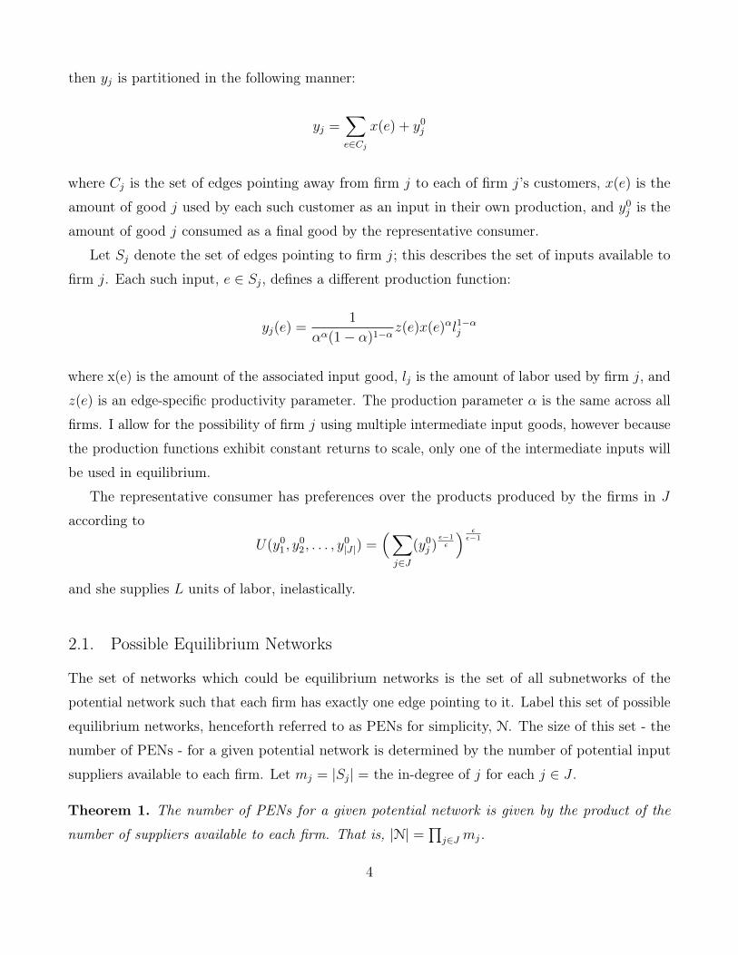
then yj is partitioned in the following manner:
yj =∑e∈Cj
x(e) + y0j
where Cj is the set of edges pointing away from firm j to each of firm j’s customers, x(e) is the
amount of good j used by each such customer as an input in their own production, and y0j is the
amount of good j consumed as a final good by the representative consumer.
Let Sj denote the set of edges pointing to firm j; this describes the set of inputs available to
firm j. Each such input, e ∈ Sj, defines a different production function:
yj(e) =1
αα(1− α)1−αz(e)x(e)αl1−αj
where x(e) is the amount of the associated input good, lj is the amount of labor used by firm j, and
z(e) is an edge-specific productivity parameter. The production parameter α is the same across all
firms. I allow for the possibility of firm j using multiple intermediate input goods, however because
the production functions exhibit constant returns to scale, only one of the intermediate inputs will
be used in equilibrium.
The representative consumer has preferences over the products produced by the firms in J
according to
U(y01, y02, . . . , y
0|J |) =
(∑j∈J
(y0j )ε−1ε
) εε−1
and she supplies L units of labor, inelastically.
2.1. Possible Equilibrium Networks
The set of networks which could be equilibrium networks is the set of all subnetworks of the
potential network such that each firm has exactly one edge pointing to it. Label this set of possible
equilibrium networks, henceforth referred to as PENs for simplicity, N. The size of this set - the
number of PENs - for a given potential network is determined by the number of potential input
suppliers available to each firm. Let mj = |Sj| = the in-degree of j for each j ∈ J .
Theorem 1. The number of PENs for a given potential network is given by the product of the
number of suppliers available to each firm. That is, |N| =∏
j∈J mj.
4
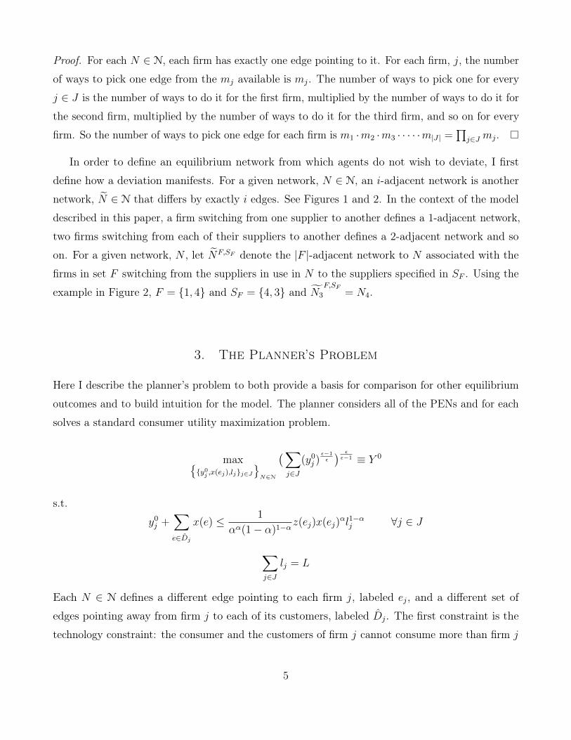
Proof. For each N ∈ N, each firm has exactly one edge pointing to it. For each firm, j, the number
of ways to pick one edge from the mj available is mj. The number of ways to pick one for every
j ∈ J is the number of ways to do it for the first firm, multiplied by the number of ways to do it for
the second firm, multiplied by the number of ways to do it for the third firm, and so on for every
firm. So the number of ways to pick one edge for each firm is m1 ·m2 ·m3 · · · · ·m|J | =∏
j∈J mj .
In order to define an equilibrium network from which agents do not wish to deviate, I first
define how a deviation manifests. For a given network, N ∈ N, an i-adjacent network is another
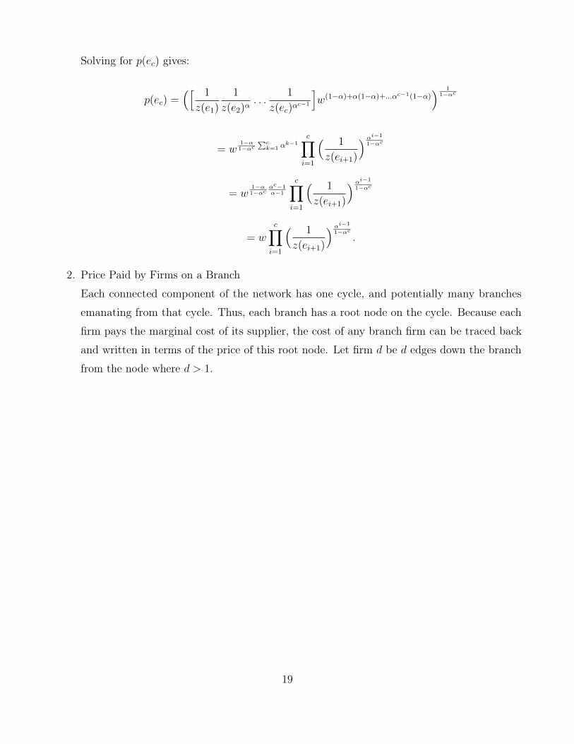
network, N ∈ N that differs by exactly i edges. See Figures 1 and 2. In the context of the model
described in this paper, a firm switching from one supplier to another defines a 1-adjacent network,
two firms switching from each of their suppliers to another defines a 2-adjacent network and so
on. For a given network, N , let NF,SF denote the |F |-adjacent network to N associated with the
firms in set F switching from the suppliers in use in N to the suppliers specified in SF . Using the
example in Figure 2, F = {1, 4} and SF = {4, 3} and N3
F,SF= N4.
3. The Planner’s Problem
Here I describe the planner’s problem to both provide a basis for comparison for other equilibrium
outcomes and to build intuition for the model. The planner considers all of the PENs and for each
solves a standard consumer utility maximization problem.
max{{y0j ,x(ej),lj}j∈J
}N∈N
(∑j∈J
(y0j )ε−1ε
) εε−1 ≡ Y 0
s.t.
y0j +∑e∈Dj
x(e) ≤ 1
αα(1− α)1−αz(ej)x(ej)
αl1−αj ∀j ∈ J
∑j∈J
lj = L
Each N ∈ N defines a different edge pointing to each firm j, labeled ej, and a different set of
edges pointing away from firm j to each of its customers, labeled Dj. The first constraint is the
technology constraint: the consumer and the customers of firm j cannot consume more than firm j
5
produces using the input defined by N . The second constraint is the labor constraint: all of the
firms in J use only the labor supplied by the representative consumer.
Each of the PENs in N defines a different maximization problem across {y0j , x(ej), lj}j∈J , each of
which the planner solves. The planner then selects the network and choice variables corresponding
to the largest Y 0. The Lagrangian for each PEN is:
L = Y 0 +∑j∈J
λj[ 1
αα(1− α)1−αz(ej)x(ej)
αl1−αj − y0j −∑e∈Dj
x(e)]+ µ[L−
∑j∈J
lj].
Define the individual efficiency of each firm, qj ≡ µλj. This will be useful in characterizing individual
and aggregate outcomes, as defined in the following theorems.
Theorem 2. In the solution to the planner’s problem the efficiency of a given firm is a function of
the efficiency of the input supplier of that firm. That is, qj = z(ej)qαs(ej)
, where s(ej) is the identity
of the input supplier used by j.
Proof. The technology constraint gives
λj =1
z(ej)λαs(ej)µ
1−α.
Using the definition of qj and then rearranging,
µ
qj=
1
z(ej)
( µ
qs(ej)
)αµ1−α
qj = µ(z(ej)
(qs(ej)µ
)α 1
µ1−α
)qj = z(ej)q
αs(ej)
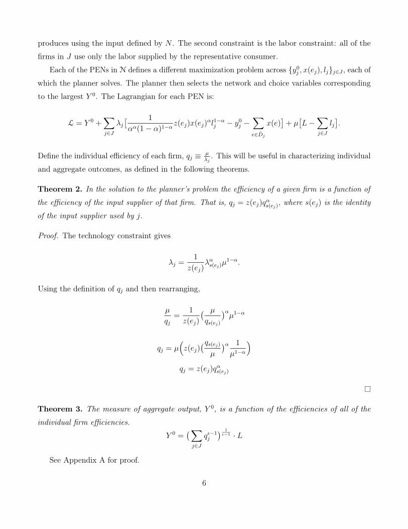
Theorem 3. The measure of aggregate output, Y 0, is a function of the efficiencies of all of the
individual firm efficiencies.
Y 0 =(∑j∈J
qε−1j
) 1ε−1 · L
See Appendix A for proof.
6

4. Equilibrium Definitions
Here I define a pairwise-stable equilibrium network and a refinement of it, a coordination-proof
equilibrium network. The definition of these require a list of payoffs for each firm for each PEN,{{π}j∈J
}N∈N. The optimal derivation of these will be described in the following section. A pairwise-
stable network is a network, N ∈ N, such that no firm j, along with any potential supplier of j,
would be made better off by moving to the 1-adjacent network defined by j and the potential supplier.
Formally, it is a network{N ∈ N : ∀j,∀k ∈ Sj \ {iNj },¬∃(j, k) s.t. πN
j,k
j > πNj and πNj,k
k > πNk},
where iNj is the supplier of firm j in N . Note that this restricts the potential firm deviations
considered. It does not allow for the individual firms to consider the possibility of the other firms
simultaneously deviating in their decision. A pairwise-stable equilibrium network merely needs to
be better than a 1-adjacent network for one pair of firms at a time. Next I define an equilibrium
network that needs to be better than i-adjacent network for i firms at a time.
A coordination-proof equilibrium network is a network, N ∈ N, such that not only no one pair
of firm and alternate supplier would be made better off by moving to the 1-adjacent network defined
by the pair, but no two pairs would be made better off, no three pairs, and so on up to the number
of firms. Let CiJ be the set of all combinations of size i of the firms in J . E.g., if J = {1, 2, 3, 4}, then
C2J =
{{1, 2}, {1, 3}, {1, 4}, {2, 3}, {2, 4}, {3, 4}
}. Let CJ =
{CiJ
}|J |i=1
. Formally, a coordination-
proof network is a network{N ∈ N : ∀Ci
J ∈ CJ ,∀j ∈ CiJ ,∀k ∈ Sj \ {iNj },¬∃(j, k) s.t. πN
j,k
j >
πNj and πNj,k
k > πNk}. Any coordination-proof network is also pairwise-stable but not necessarily
vice-versa. Therefore, the number of coordination-proof networks will be less than or equal to the
number of pairwise-stable networks.
5. Prices and Profit Maximization
When exactly one edge is pointing to each firm, there are only two possible network shapes that
can make up each connected component of the entire network. These are cycles and branches. A
cycle is a set of nodes such that the in-degree and out-degree of each node is exactly one. A branch
is a set of nodes such that the in-degree of each node is one but the out-degree is unrestricted.
See Figure 3. Any connected component must contain exactly one cycle and any branch in that
7

connected component must have its root on the cycle.1 These two shapes are critical in calculating
the prices.
Firms set prices for both the portion of their output consumed by the representative consumer
and the portion consumed by each of their network customers - the other firms which use their
good as an input. Label the price of y0j as p0j . For each network customer of firm j, j charges a
two-part tariff. That is, j sets {p(e), τ(e)}e∈Dj , for each Dj defined by each N ∈ N. Here τ(e) is
fixed fee and p(e) is a price per unit of product j.
Theorem 4. The per-unit price, p(e), that firm j charges the customer to which edge e points is
firm j’s marginal cost of production.
See Appendix C for proof. As a result of this, the per-unit price firm j charges is a function of
the marginal cost of the input supplier used by firm j, p(e) =MCj =1
z(ej)MCs(ej)w
1−α, where w is
the price of labor to all firms. Because the price charged by each firm can be written in terms of
the supplier’s marginal cost, all of these prices can be calculated using only the network structure
and z(ej)’s. The price charged by any firm on a cycle can be traced back through each supplier
until it is expressed in terms of itself, thus there is a closed form solution for any price on a cycle.
The price charged by any firm on a branch can be traced up to the root node of the cycle, which
must be on a cycle, thus any such price can be calculated. See Appendix C for formal derivation.
The profit maximization problem each firm j solves is
maxp0j ,y
0j ,x(ej),lj
p0jy0j +
∑e∈Dj
[p(e)x(e) + τ(e)]− [p(ej)x(ej) + τ(ej)]− wlj
s.t.
y0j +∑e∈Dj
x(e) ≤ 1
αα(1− α)1−αz(ej)x(ej)
αl1−αj
and all firms are jointly subject to the labor constraint,∑
j∈J lj = L.
Each N ∈ N defines a different profit maximization problem for each firm and the solutions to
these produce a set of payoffs for each firm for each PEN. These payoffs are what determine the
pairwise-stable and the coordination-proof equilibria, as defined in the previous section.
Just as the efficiency of an individual firm in the planner’s problem is defined as the ratio of the1If it had no cycle then there would need to exist one node with no supplier and if there was more than one cycle
then there would exist some node with more that one supplier.
8
two shadow costs µ and λj, define the efficiency of the individual firms in this case as, qj ≡ wMCj
.
As in the case of the planner’s problem, this can be written in terms of the efficiency of firm j’s
input supplier.
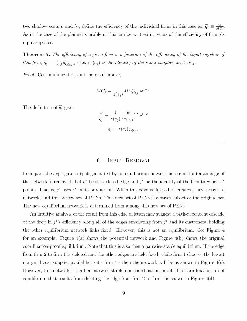
Theorem 5. The efficiency of a given firm is a function of the efficiency of the input supplier of
that firm, qj = z(ej)qαs(ej)
, where s(ej) is the identity of the input supplier used by j.
Proof. Cost minimization and the result above,
MCj =1
z(ej)MCα
s(ej)w1−α.
The definition of qj gives,w
qj=
1
z(ej)
( w
qs(ej)
)αw1−α
qj = z(ej)qs(ej).
6. Input Removal
I compare the aggregate output generated by an equilibrium network before and after an edge of
the network is removed. Let e∗ be the deleted edge and j∗ be the identity of the firm to which e∗
points. That is, j∗ uses e∗ in its production. When this edge is deleted, it creates a new potential
network, and thus a new set of PENs. This new set of PENs is a strict subset of the original set.
The new equilibrium network is determined from among this new set of PENs.
An intuitive analysis of the result from this edge deletion may suggest a path-dependent cascade
of the drop in j∗’s efficiency along all of the edges emanating from j∗ and its customers, holding
the other equilibrium network links fixed. However, this is not an equilibrium. See Figure 4
for an example. Figure 4(a) shows the potential network and Figure 4(b) shows the original
coordination-proof equilibrium. Note that this is also then a pairwise-stable equilibrium. If the edge
from firm 2 to firm 1 is deleted and the other edges are held fixed, while firm 1 chooses the lowest
marginal cost supplier available to it - firm 4 - then the network will be as shown in Figure 4(c).
However, this network is neither pairwise-stable nor coordination-proof. The coordination-proof
equilibrium that results from deleting the edge from firm 2 to firm 1 is shown in Figure 4(d).
9

While in the case of a solution to the planner’s problem, the new output will be lower than the
original output, this is not necessarily true in the case of a new pairwise-stable equilibrium, and, in
fact, this result survives the equilibrium refinement of the coordination-proof equilibrium.
Result 1. There exist parameters of the model such that the output produced by a pairwise-stable
equilibrium or by a coordination-proof equilibrium increases when an edge is deleted and a new
equilibrium of the same type is determined.
See Figure 5 for an example. Figure 5(a) shows the potential network and Figure 5(b) shows
the original coordination-proof (and pairwise-stable equilibrium) network in which output is 0.0371.
When the edge from firm 4 to firm 3 is deleted, the new equilibrium is shown in Figure 5(c) in
which output is 0.2921.
6.1. Network Connectivity and Firm Centrality
To avoid overly cumbersome phrasing, I restrict my focus to the situation in which output falls
when an edge is deleted. These results hold in the case that output rises, as well. The connectivity
of the equilibrium network as a whole plays a roll in how far aggregate output falls after an edge
is deleted. The intuitive relationship may be that the more connected an equilibrium production
network is, the harder each firm will be hit when j∗ loses its input supplier and has to choose
a different one, and this aggregate output will drop by more when a network is more connected.
While the simulations described in the next section show that on average this is the case, the
opposite may also occur.
Result 2. There exist parameters of the model such that higher connectivity in an original equilib-
rium network can lead to a smaller decrease in aggregate output.
See Figures 6 and 7 for an example. In the first potential network, shown in Figure 6(a), firm
2 has two available suppliers and in the second potential network, Figure 6(b), firm 2 has three
available suppliers. Figure 6(c) shows the coordination-proof equilibrium they have in common, in
which output is 0.1430. When the edge from firm 4 to firm 2 is deleted from both of them, the
resulting new coordination-proof equilibria are shown in Figure 7(a) and Figure 7(b), respectively.
The output in the first one is 0.0371, while the output in the second one is 0.0356.
Just as the connectivity of the network as a whole affects the drop in output, the level of
connectedness, or centrality, of j∗ in the potential network, as measured by the number of alternative
10
suppliers available to j∗, plays a roll as well. As one might expect, the average outcome is that if
j∗ has more alternative suppliers to choose from when it looses its equilibrium input supplier, the
drop in aggregate output will be smaller than if j∗ had fewer alternative suppliers. However, the
opposite effect is possible.
Result 3. There exist parameters of the model such that a higher number of alternative suppliers
for j∗ can lead to a larger drop in aggregate output.
See Figures 8 and 9 for an example. The network in Figure 8(a) is less connected than the
network in Figure 8(b); however when the edge from firm 4 to firm 2 is deleted from both of them,
the output in the less connected network decreases more.
7. Simulation Results
I simulate this model by generating potential production networks and then finding a solution to
the planner’s problem, a pairwise-stable equilibrium, and a coordination proof equilibrium. I create
the potential network by drawing a number of possible input suppliers for each from a Poisson(3)
distribution. The identity of each supplier is drawn uniformly with replacement from the other firms.
The productivity parameter, z(e), for each edge e is drawn from a Pareto(0.2,−1.8) distribution.This parameterization is motivated by the Carvalho (2012) survey on Input-Output analysis. Note
that drawing the supplier identities with replacement allows for multiple edges from a given firm.
However, because the productivity parameters are realizations of continuous random variables, the
edge with the higher z will always be chosen. These simulations consisted of the creation of 1, 000
potential networks, in 512 of which a solution to all three problems was found.
7.1. Removal of an Input Supplier
For each successful solution to the planner’s problem, pairwise-stable equilibrium, and coordination-
proof equilibrium determination, I delete each edge in use in equilibrium. I do this by removing
that edge from the potential network and then find a new solution of each type. In 2, 536 of these
edge deletion experiments, a new solution to all three allocations is found. I take the ratio of output
after the edge is deleted to output before the edge is deleted. Label this relative output for each
allocation: planner, pairwise-stable, and coordination-proof.
I measure the connectivity of each original equilibrium using the average shortest path distance.
11
I do this by calculating the length of the directed path from each node to every other node and
taking the average across all such paths. A larger average shortest path distance corresponds
to a less connected network and a shorter average shortest path distance corresponds to a more
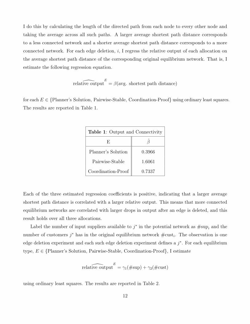
connected network. For each edge deletion, i, I regress the relative output of each allocation on
the average shortest path distance of the corresponding original equilibrium network. That is, I
estimate the following regression equation.
relative outputE= β(avg. shortest path distance)
for each E ∈ {Planner’s Solution, Pairwise-Stable, Coordination-Proof} using ordinary least squares.
The results are reported in Table 1.
Table 1: Output and Connectivity
E β
Planner’s Solution 0.3966
Pairwise-Stable 1.6061
Coordination-Proof 0.7337
Each of the three estimated regression coefficients is positive, indicating that a larger average
shortest path distance is correlated with a larger relative output. This means that more connected
equilibrium networks are correlated with larger drops in output after an edge is deleted, and this
result holds over all three allocations.
Label the number of input suppliers available to j∗ in the potential network as #supi and the
number of customers j∗ has in the original equilibrium network #custi. The observation is one
edge deletion experiment and each such edge deletion experiment defines a j∗. For each equilibrium
type, E ∈ {Planner’s Solution, Pairwise-Stable, Coordination-Proof}, I estimate
relative outputE= γ1(#sup) + γ2(#cust)
using ordinary least squares. The results are reported in Table 2.
12

Table 2: Output and Centrality
E γ1 γ2
Planner’s Solution 0.2626 0.0382
Pairwise-Stable 0.9249 0.4786
Coordination-Proof 0.4728 0.0998
The estimated regression coefficients on the number of available suppliers are positive for all three
equilibrium definitions. This indicates that a larger number of available input suppliers is correlated
with a smaller drop in output after an edge is deleted.
The estimated regression coefficients on the number of customers in the original equilibrium
network are all positive as well, indicating the more customers j∗ has when it loses its input supplier,
the higher output will be afterwards. However, in the case of the coordination-proof equilibrium
the confidence interval of γ2 includes zero, and this was true for every size of simulation. While it
may be the case that in the planner’s problem and in pairwise-stable networks, a larger number
of customers is correlated with a smaller drop in aggregate output, this cannot be concluded for
coordination-proof networks.
8. Conclusion
The key contributions of this paper are a new network model which features a finite number of firms
and endogenous network determination, a refinement of the standard network equilibrium, and a
better understanding of the role network connectivity and firm centrality play in the determination
of aggregate outcomes. Simulation results indicate the following. First, on average, the more
connected a production network is, the smaller the decrease in aggregate output will be when a
firm loses an input supplier. Second, on average, the more alternative suppliers that firm has, the
smaller the drop in output will be when that firm loses its input supplier.
References
[Acemoglu et al., 2012] Acemoglu, Daron, Carvalho, Vasco M., Ozdaglar, Asuman, and Tahbaz-
Salehi, Alireza. (2012). The Network Origins of Aggregate Fluctuations. Econometrica. Vol.
13

80 No. 5
[Baqaee, David Rezza, 2013] Baqaee, David Rezza. (2013). Cascading Failures in Production
Networks. London School of Economics and Political Science.
[Carvalho and Voigtländer, 2015] Carvalho, Vasco M. and Voigtländer, Nico. (2015). Input Diffu-
sion and the Evolution of Production Networks. Economic Working Papers 1418
[Chartrand, 1977] Chartrand, Gary. (1977). Introductory Graph Theory. Dover Publication. New
York, NY.
[Dalal et al., 2008] Dalal, Ishaan L., Stefan, Deian, and Harwayne-Gidansky, Jared. (2008). Low
Discrepancy Sequences for Monte Carlo Simulations on Reconfigurable Patters. Application-
Specific Systems, Architectures and Processors, 2008. ASAP 2008. International Conference
on. IEEE, 2008
[di Giovanni et al., 2014] di Giovanni, Julian, Levchenko, Andrei A., and Mejean, Isabelle. (2014).
Firms, Destinations, and Aggregate Fluctuations. Econometrica. Vol. 82 No. 4
[Dupor, 1999] Dupor, Bill. (1999). Aggregation and Irrelevance In Multi-Sector Models. Journal
of Monetary Economics Vol. 43 Issue 2
[Hildenbrand and Kirman, 1988] Hildenbrand, W. and Kirman, A.P. (1988). Equilibrium Analysis.
Elsevier Science Publishers B.V. Princeton, NJ.
[Herman, 2006] Herman, Charles. (2006). Katrina’s Economic Impact: One Year Later. ABC
News.
[Horvath, 1998] Horvath, Michael. (1998). Cyclicality and Sectoral Linkages: Aggregate Fluc-
tuations from Independent Sectoral Shocks. Review of Economic Dynamics. Vol. 1 Issue
4
[Jackson, 1988] Jackson, Matthew O. (2008). Social and Economic Networks. Princeton University
Press. Amsterdam, The Netherlands
[Oberfield, 2013] Oberfield, Ezra. (2013). Business Networks, Production Chains, and Productivity:
A Theory of Input-Output Architecture. Working Paper Series Federal Reserve Bank of
Chicago, WP-2011-12.
14
[PBS Newshour] “How a sophisticated malware attack is wreaking havoc on Ukraine." PBS
Newshour, PBS. WETA, Washington, D.C. 28 June 2017. Television.
[Tucker, 2007] Tucker, Alan. (2007). Applied Combinatorics. John Wiley and Sons. Hoboken, NJ.
9. Appendix A: The Planner’s Problem
9.1. Proof of Theorem 3: Aggregate Output and Efficiency
Each firm j uses a number of supply chains in the production process. A supply chain is a string of
firms, each producing intermediate goods for the next firm in the chain. Label the set of supply
chains which lead to firm j as Sj. Partition firm j’s final output, y0j , by final output produced by
each supply chain, s ∈ Sj. That is,∑
s∈Sj y0j (s) = y0j . To make y0j (s), firm j uses labor l0j (s) ≤ lj
and intermediate input x0j(s) ≤ xj. This x0j(s) is produced by firm j’s supplier using l1j (s) and
x1j(s), this x1j(s) is produced using l2j (s) and x2j(s), and so on up the supply chain. In general, I
write lk+1j (s) and xk+1
j (s) are the labor and intermediate input amounts used to make xkj (s), along
supply chain s to make firm j’s output for final consumption. The lower subscript describes the
good at the end of the supply chain and the superscript describes the step up the supply chain,
Let λ0j(s) be the marginal social cost of producing x0j(s) and let µ be the marginal social cost of
labor, following the earlier notation. The optimal choices of x0j(s) and l0j (s) give:
λkj (s)xkj (s)
α=wlkj (s)
1− α
λk+1j (s)xk+1
j (s)
α=wlk+1
j (s)
1− α.
Using the technological constraint,
λj =1
z(ej)λαs(ej)µ
1−α
where s(ej) is the supplier of edge ej . This means that the marginal social cost of producing product
j is determined by the marginal social cost of firm j’s supplier. This will be necessary for connecting
efficiency across the entire network. The network structure gives λk+1j (s)xk+1
j (s) = αλkj (s)xkj (s), so
15
the optimality condition for the (k + 1)th step up the supply chain becomes λkj (s)xkj (s) =wlk+1j (s)
1−α .
Substituting this into the optimality condition for the kth step gives lk+1j (s) = αlkj (s). That is, the
labor used in each step along the supply chain to make intermediate goods for y0j (s) is a constant
share of the labor used in the previous step.
Let lj(s) be the total labor used along supply chain s to make y0j (s) such that lj(s) =∑∞
k=1 lkj (s) =∑∞
k=1 αkl0j (s) =
l0j (s)
1−α . From the optimality condition for the final step in the supply chain,
λjy0j (s) =
wl0j (s)
1− α= wlj(s).
Finally, write y0j =∑
s∈Sj y0j (s) =
∑s∈Sj
wλjlj(s) =
wλj
∑s∈Sj lj(s) =
wλjlj. From the definition of qj,
I can now write y0j = qjlj.
From here, I use the solution to this planner’s problem to show that Y 0 = L[∑J
j=1 qε−1j
] 1ε−1 . Let[∑Jt
j=1 qε−1j
] 1ε−1 ≡ Q. First, the first order condition with respect to firm y0j is
(Y 0) 1ε (y0j )
− 1ε = λj.
Rearranging this gives λj =(y0jY 0
)− 1ε . This expression can be used to show that
∑Jtj=1 λ
1−εj = 1.
Rewriting the definition of firm efficiency for qj allows me to write∑Jt
j=1
(wqj
)1−ε= 1. Then,
using the definitions of qj and Q, I can write y0jY 0 =
(qjQ
)ε.
Finally, I use the labor constraint to show L =∑Jt
j=1
(lj
)=∑Jt
j=1
(y0jqj
)= Y 0Q−ε
∑Jtj=1 q
ε−1j =
Y 0Q−εQε−1 = Y 0
Q. Rewritten, this is the expression I need: Y 0 = QL.
10. Appendix B: Equilibrium
10.1. Existence of a Solution to Each Agents’ Problem
I use the Theorem of the Maximum to show that the individual agents’ problems each have a
solution. Recall that the optimization process proceeds as follows: taking the set of inputs that are
used and their associated two-part prices as given, firms maximize profits by choosing the price for
final output, poj , the amount of final output, yoj , the amount of the intermediate good they use, xj,
and the labor they use, lj. Then the firms choose their optimal input and the two-part prices they
charge their potential customers, that is, the set of edges that are used in the production network,
E, and prices for each edge, {p(e), τ(e)}e∈E.The objective function is certainly continuous, so I focus here on the compactness and continuity
16

of the constraint correspondence. Each firm must choose prices for each technique for which they
are a supplier. These prices are drawn from compact and continuous sets. These prices in turn
continuously determine the budget sets for the firms. Note that for each possible input choice,
there is a set of four choice variables, poj , yoj , xj , and lj , each of which is chosen from a compact and
continuous correspondence determined by the budget sets.
The constraint correspondence is therefore the finite Cartesian product of compact and continu-
ous correspondences and is therefore compact and continuous. Thus, the Theorem of the Maximum
applies and each agent’s problem has a solution.
Given that each agent has a solution to her maximization problem, and that in each time period
there is a finite number of agents, Kakutani’s Fixed Point Theorem applies and there exists a Mixed
Strategy Nash Equilibrium in each time period.
11. Appendix C: Prices
11.1. Pricing at Marginal Cost
Proposition: The per-unit price, p(e), that firm j charges to firm i along edge e is the marginal
cost of firm j, MCj.
Proof: Following Oberfield (2013), suppose for the purpose of contradiction that firm j charges
some other price, p(e) = p 6=MCj. Label the associated contract (p, τ).
Consider the deviation from (p, τ), p(e) = p = MCj and τ(e) = τ = τ + (p−MCj)x(e) +K,
where
K =1
2
{(p0i − ci)y0i − (p0i − ci)y0i +
∑e∈Di
(p(e)− ci)[xb(e)(y0i )− xb(e)(y0i )]}
and ci = 1z(e)
MCαj w
1−α, the marginal cost of i given the deviation. I will show that both firm j
and firm i are made better off by this deviation and thus (p, τ) is not optimal.
First, πj − πj = K > 0.
Next, πi − πi = p0i y0i − p0i y0i +
∑e∈Di p(e)[xb(e)(y
0i )− xb(e)(y0i )]− [ciyi − ciyi]− [τ − τ ]. By using,
(i) p(e)x(e) = αciyi and (ii) cici=(p(e)cj
)α, I can write:
πi − πi =
17

(p0i − ci)y0i − (p0i − ci)y0i +∑e∈Di
(p(e)− ci)[xb(e)(y0i )− xb(e)(y0i )]−K
+[((1− α) + MCj
p(e)α)( p(e)MCj
)α − 1]ciyi.
By the definition of K, the first line of the equation is positive. Jensen’s Inequality gives that
[(1− α) + xα]x−α ≥ 1 for α ∈ [0, 1]. Applying this to the second line of the equation gives that
[(1− α) + MCjp(e)
α](p(e)/MCj)α ≥ 1, so the second line of the equation is non-negative. As a result,
πi − πi is postive and both firm i and firm j are made better off by firm j charging MCj.
11.2. Derivation of Price Expressions
Both of the following derivations are driven by the fact that the price that each firm pays for each
unit of the input they use is the marginal cost of the supplier of that input, as proved above.
1. Price Paid by Firms on a Cycle
For a cycle of length c, there are c firms and c edges. Label these firms 1, . . . , c. Without loss
of generality, we find the price of firm c and label the supplier c uses as 1, the supplier 1 uses
as 2 and so on.
1
2
3
c
z(ec)z(e1)
z(e2) z(e3)
The price that c pays for its input is p(ec) = 1z(e1)
p(e1)αw1−α, where p(e1) is the price firm
1 pays for its input. This price is p(e1) = 1z(e2)
p(e2)αw1−α, where p(e2) is the price firm 2
pays for its input. Continuing in this way I can write the price that firm c − 1 pays as
p(ec−1) =1
z(ec)p(ec)
αw1−α. Substituting each price expression into the previous one gives:
p(ec) = p(ec)αc[ 1
z(e1)
1
z(e2)α. . .
1
z(ec)αc−1
]w(1−α)+α(1−α)+...αc−1(1−α).
18
Solving for p(ec) gives:
p(ec) =([ 1
z(e1)
1
z(e2)α. . .
1
z(ec)αc−1
]w(1−α)+α(1−α)+...αc−1(1−α)
) 11−αc
= w1−α1−αc
∑ck=1 α
k−1c∏i=1
( 1
z(ei+1)
) αi−1
1−αc
= w1−α1−αc
αc−1α−1
c∏i=1
( 1
z(ei+1)
) αi−1
1−αc
= w
c∏i=1
( 1
z(ei+1)
) αi−1
1−αc.
2. Price Paid by Firms on a Branch
Each connected component of the network has one cycle, and potentially many branches
emanating from that cycle. Thus, each branch has a root node on the cycle. Because each
firm pays the marginal cost of its supplier, the cost of any branch firm can be traced back
and written in terms of the price of this root node. Let firm d be d edges down the branch
from the node where d > 1.
19

2
3
c
1
b1
b2
d b3
z(e1)z(e2)
z(e3) z(ec)
z(eb1)
z(eb2)
z(eb3)
z(ed)
The price that d pays for its input is the marginal cost of its supplier. The price the supplier
pays is the marginal cost of his supplier and so on up to the root node, whose price was found
in the above derivation. Label MCr =1
z(er)pαrw
1−α. Then the price that firm d pays is
p(ed) =MCαd−1
r
[ d−1∏i=1
1
z(ebi)αd−i−1
]w(1−α)
∑d−2k=0 α
k
=MCαd−1
r
[ d−1∏i=1
1
z(ebi)αd−i−1
]w(1−α)α
d−1α−1
=MCαd−1
r
[ d−1∏i=1
1
z(ebi)αd−i−1
]w1−αd .
For a firm that is only one edge away, for example firm b1 in the figure, the price that firm
pays is the marginal cost of the root node, MCr.
20

12. Figures
Figure 1: Network N1 is 1-adjacent to N2 and vice versa.
1 2
3 4(a) N1
1 2
3 4(b) N2
21
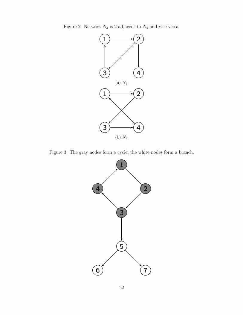
Figure 2: Network N3 is 2-adjacent to N4 and vice versa.
1 2
3 4(a) N3
1 2
3 4(b) N4
Figure 3: The gray nodes form a cycle; the white nodes form a branch.
1
2
3
4
5
6 7
22

Figure 4: Deleting an edge and holding the other edges fixed is not neccessarily an equilibrium
1 2
3 4
0.17
8.49
2.93
0.51
0.68
0.25
1.19
0.10
(a) Potential Network
1 2
3 4
8.49
0.51
0.680.10
(b) Original Equilibrium Network
1 2
3 4
0.51
0.680.10
0.25
(c) Holding other edges fixed
1 2
3 4
2.93
0.68
1.190.25
(d) The equilibrium network when the edge is deleted
23

Figure 5: Output increases when the edge from firm 4 to firm 3 is deleted.
1 2
3 4
0.17
8.49
2.93
0.51
0.68
0.25
1.19
0.10
(a) Potential Network
1 2
3 4
8.49
0.51
0.680.10
(b) Original Equilibrium Network, Output = 0.0371
1 2
3 4
8.49
2.93
0.51
0.68
(c) New Equilibrium, Output= 0.2921
24

Figure 6: Output goes down by more when firm 2 has more alternative suppliers.
1 2
3 4
0.17
8.49
2.93
0.51
0.68
0.25
1.19
0.10
(a) Potential Network #1, Firm 2 has two available suppliers.
1 2
3 4
0.17
0.83
8.49
2.93
0.51
0.68
0.25
1.19
0.10
(b) Potential Network #2, Firm 2 has three available suppliers.
1 2
3 4
2.93
0.68
1.190.25
(c) Original Equilibrium Network, Output = 0.1430
25

Figure 7: Output goes down by more when firm 2 has more alternative suppliers.
1 2
3 4
8.49
0.51
0.680.10
(a) New Equilibrium for Potential Network #1,Output= 0.0371
1 2
3 4
0.83
0.172.93
0.25
(b) New Equilibrium for Potential Network #2,Output= 0.0356
Figure 8: Output goes down less for the more connected network.
1 2
3 4
8.49
0.68
1.19
0.10
(a) Original Equilibrium #1, Output= 0.0452, Avg.Path Distance= 1.6875
1 2
3 40.68
8.49 1.19
0.10
(b) Original Equilibrium #2, Output= 0.0445, Avg.Path Distance= 1.5
Figure 9: Output goes down less for the more connected network.
1 2
3 4
8.49
0.51
0.680.10
(a) New Equilibrium #1, Output= 0.0371
1 2
3 4
0.17
2.938.49
0.51
(b) New Equilibrium #2, Output= 0.1854
26