Employment Industry and Occupational Continuity in …ftp.iza.org/dp8372.pdf · Employment Industry and Occupational Continuity in Germany: ... Miracle (Wirtschaftswunder). This comparison

DI

SC

US

SI

ON

P

AP

ER

S

ER

IE

S

Forschungsinstitut zur Zukunft der ArbeitInstitute for the Study of Labor

Employment Industry and Occupational Continuity in Germany: From the Nazi Regime to thePost-War Economic Miracle

IZA DP No. 8372

August 2014

Patrick A. Puhani

Employment Industry and Occupational Continuity in Germany: From the Nazi

Regime to the Post-War Economic Miracle

Patrick A. Puhani Leibniz University of Hannover,

SEW, University of St. Gallen and IZA

Discussion Paper No. 8372 August 2014

IZA

P.O. Box 7240 53072 Bonn

Germany

Phone: +49-228-3894-0 Fax: +49-228-3894-180

E-mail: [email protected]

Any opinions expressed here are those of the author(s) and not those of IZA. Research published in this series may include views on policy, but the institute itself takes no institutional policy positions. The IZA research network is committed to the IZA Guiding Principles of Research Integrity. The Institute for the Study of Labor (IZA) in Bonn is a local and virtual international research center and a place of communication between science, politics and business. IZA is an independent nonprofit organization supported by Deutsche Post Foundation. The center is associated with the University of Bonn and offers a stimulating research environment through its international network, workshops and conferences, data service, project support, research visits and doctoral program. IZA engages in (i) original and internationally competitive research in all fields of labor economics, (ii) development of policy concepts, and (iii) dissemination of research results and concepts to the interested public. IZA Discussion Papers often represent preliminary work and are circulated to encourage discussion. Citation of such a paper should account for its provisional character. A revised version may be available directly from the author.

mailto:[email protected]

IZA Discussion Paper No. 8372 August 2014

ABSTRACT

Employment Industry and Occupational Continuity in Germany: From the Nazi Regime to the Post-War Economic Miracle*

Using retrospective survey data that covers 1939, 1950, 1960, and 1971, I compare individual-level changes in employment industry and occupational status in Germany from the beginning of World War II to the post-war reconstruction era dubbed the Economic Miracle (Wirtschaftswunder). This comparison reveals that, with only a few exceptions, labor allocation developments remained relatively stable even in the face of huge political and macroeconomic change. JEL Classification: N34, J01 Keywords: employment, evolution, regime change, revolution, Germany, Arab Spring,

Iraq Corresponding author: Patrick A. Puhani Leibniz Universität Hannover Institut für Arbeitsökonomik Königsworther Platz 1 D-30167 Hannover Germany E-mail: [email protected]

* I thank Knut Gerlach, Olaf Hübler, Bernhard Schimpl-Neimanns, Alexander Straub, Stephan Thomsen, and Reinhard Weisser for helpful comments and GESIS Mannheim for providing access to the Mikrozensus 1971 data set.

mailto:[email protected]

1

1 Introduction After every major regime change, be it the fall of communism or the Arab Spring, the

new regime must decide on the extent to which it should replace major and minor players in

both public administration and the private sector. Germany presents a particularly interesting

case for studying this phenomenon because after a war that left the country morally and

economically devastated, the post-war reconstruction in its western part (the Federal

Republic) is generally seen as both a political and economic success. I thus investigate the

issue of post-regime changes phenomenon by comparing individual career paths during two

historical periods: WWII and the post-war reconstruction era. Specifically, using person-level

data from a 1971 retrospective survey, I derive measures of association for employment

industry (the worker’s sector of employment) and occupational status for the same

individuals at the beginning and end of the 1939–1950 decade (which includes WWII) and

the 1950–1960 and 1960–1971 post-war decades in democratic West Germany. I then

perform a comparative analysis that documents a high degree of continuity in the German

labor market before and after World War II; that is, changes in individual careers in the

WWII era greatly resemble those in the post-war decades.

Even during WWII, when the Nazi regime restricted personal and economic freedoms

considerably or removed them completely, some elements of a market economy still

persisted in Germany. The stock exchange, for example, remained open, although the regime

froze stock prices at the beginning of 1943 and often “outsourced” state enterprise (including

racially or politically motivated expropriations) to private businesses (Aly, 2011). Not that

advice was lacking on the benefits of competition (Schmölders, 1942): even after the Soviets

had defeated the German Sixth Army at Stalingrad (generally seen as a turning point of

WWII), German economist Günter Schmölders (1943) expressed concern about changes in

the tax system not sufficiently rewarding entrepreneurial success.

In fact, the German war economy relied heavily on resources (including food and

forced labor) drawn from occupied territories (Aly, 2011), meaning that toward the end of the

war and during the years immediately following it, economic breakdown occurred. As

Hirshleifer (1963) notes, “[t]ransportation had generally stopped, and with it practically all

industrial production” (p. 84). Immediately after the war, the German economy still faced

price restraints implemented in the pre-war period to address excess money supply, as well as

a division into four occupation zones (with trade restrictions between them), loss of territory

east of the Oder-Neisse line, a housing and refugee problem, and the temporary cessation of

regular foreign trade. Beginning in 1948, however, currency reform, the return of about 1

2

million remaining prisoners of war from the western Allied powers (Hirshleifer, 1963), and

the establishment of support and cooperation between these powers and the new West

Germany initiated a period of economic growth that Germans still refer to as the Economic

Miracle (Wirtschaftswunder).

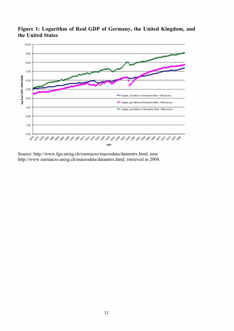
To put these developments into a macroeconomic perspective, Figure 1 displays the

log of GDP for (West) Germany, the UK and the U.S. from 1870 (the year before German

unification under Bismarck) until 1989 (the year the Berlin Wall was toppled and one year

before German reunification). As the figure shows, all three economies recovered from the

two world wars and the Great Depression along a steady growth path, and all were

characterized by significant long-term growth. In fact, a projection of pre-1914 growth trends

into the future shows that not only for the U.S. but also for Germany, the country that lost

both world wars, GDP seems to have caught up to its pre-WWI trend. Yet even beyond this

exceptionally high growth rate in the aftermath of WWII, what is probably most remarkable

about Germany’s Economic Miracle is that the country not only made up for wartime GDP

losses but also shot back up to a GDP growth trajectory that could have been expected in

1914. In other words, despite the damage to GDP growth inflicted by WWII, WWI, and the

Great Depression (ranked in order of perceived seriousness), the country’s economy bounced

back almost as though these disasters had never happened (see also Brakman, Garretsen, and

Schramm, 2004; Davis and Weinstein 2002; and Miguel and Roland, 2011 on bombing and

recovery of Germany, Japan, and Vietnam, respectively).

What, then, can account for the Economic Miracle? First, as Hirshleifer (1963) points

out, the destruction of productive physical capital was lower than suggested by pictures of

destroyed inner cities: post-war industrial capacity was actually only 20 percent below its

pre-war level. Second, as both Hirshleifer (1963) and Waldinger (2012) stress, even in the

face of the housing crisis and loss of life, the human capital brought to West Germany by the

survivors, including the 8–10 million German refugees from Eastern Europe (Ritschl, 2005,

p.152), was more important than physical capital. That is, despite Nazi destruction of life and

human capital—begun even before the war with, for example, the racially or politically

motivated expulsion of talent from the universities (Waldinger, 2010)—and the war’s own

toll on human capital through reduced education for specific birth cohorts (Ichino and

Winter-Ebmer, 2004), human capital played a major role in the recovery. Most particularly,

as shown in this note, for the cohorts less affected by active military service, the years

between 1939 and 1950 are marked by a large degree of individual-level continuity in terms

of employment industry and occupational status.

3

2 Data and Cohorts Unfortunately, individual data from the pre-WWII period in Germany were lost when

the census punch cards were destroyed. However, the 1971 West German Labor Force

Survey (Mikrozensus) asks retrospective questions on employment industry and occupational

status during 1939, 1950, 1960, and 19711 that enable the tracking of individual employment

industry and occupational status dynamics for over 30 years. The purpose of this note,

therefore, is to draw on this person-level data to document individuals’ employment industry

and occupational status just before and shortly after WWII (i.e., from 1939 to 1950) and

compare it to that in two decades of comparatively high economic and political stability (i.e.,

1950–1960 and 1960–1971). To control for younger cohorts whose lives and careers were

massively perturbed (if not lost) during the war, the comparison focuses on birth cohorts who

already had some work experience at the outbreak of war and were thus less affected by the

draft. That is, even though age groups 18 to 45 were subject to conscription and heavily

recruited early in the war (Absolon, 1960, p. 153), men older than 30 found it easier to obtain

“indispensable” (unabkömmlich) status (e.g., as war industry workers, administrators, and in

some cases, even as celebrities), which allowed them to continue in their civil jobs.2 For these

men, this status was granted for at least 3 months and had to be actively renounced by the

recruitment office, whereas for younger men, the maximum “indispensable” period was only

3 months (Absolon, 1960, p. 142).3

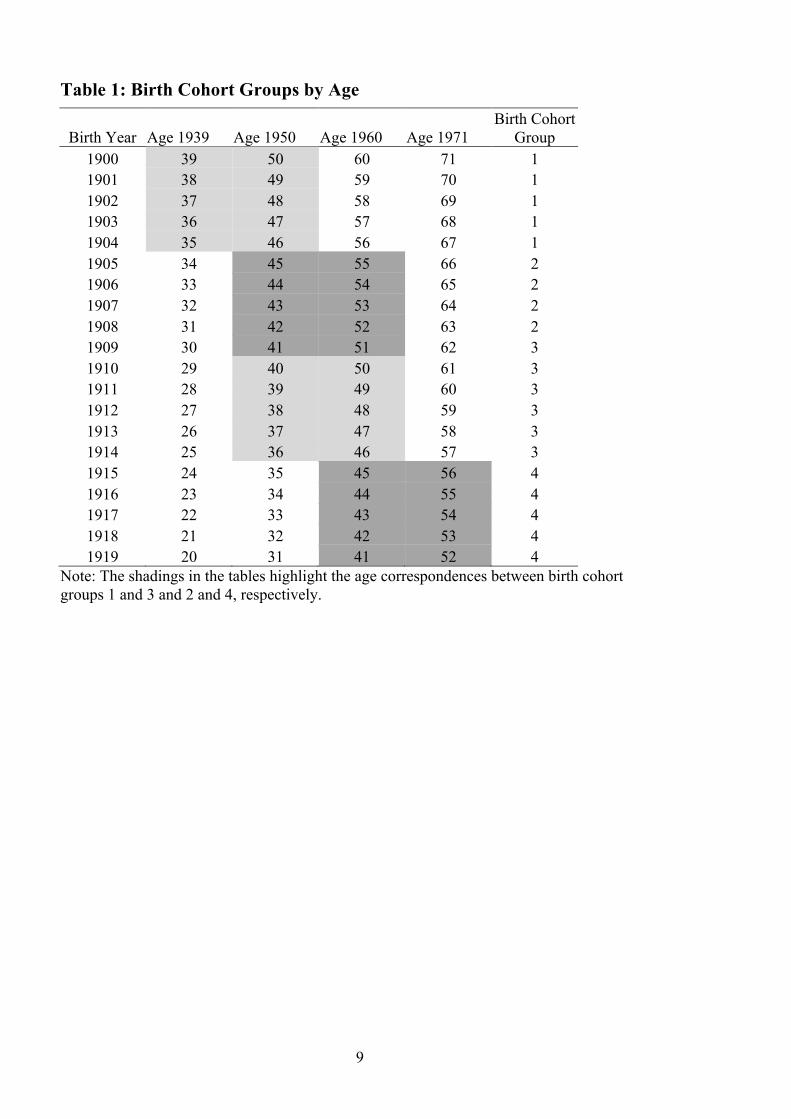
Table 1 defines the four birth cohort groups used in this analysis and shows their

respective ages in the observation years 1939 to 1971. Correspondence between the groups is

generated by the age range observed for each pair of two birth cohort groups. For example,

Group 1, born between 1900 and 1904, transits from being between 35 and 39 years old to

being between 46 and 50 years old between 1939 and 1950, while Group 3, born between

1910 and 1914, experiences (almost) these exact ages a decade later, between 1950 and 1960.

Likewise, Group 2, born between 1905 and 1909, is aged between 30 and 34 (41 and 45) in

1 The data source is documented in http://www.gesis.org/missy/missy-home/auswahl-

datensatz/mz-zusatzerhebung-1971/ 2 In October 1944, conscription into the National Militia (Volkssturm) was extended to age

groups 16 to 60 (source: http://de.wikipedia.org/wiki/Volkssturm). 3 Absolon (1960) does not stipulate which share of the male population was able to obtain

“indispensable” status. However, Abolon (1960) reports that as of November 7 1943 (after the battle of Stalingrad), the German army had deployed 7,228,300 people at a front length of 15,250 km in Europe. Compare that to a population of 79,375,281 reported in the census of 1939 (which included Austria and parts of Czechoslovakia; source: http://de.wikipedia.org/wiki/Liste_der_Volkszählungen_in_Deutschland).

4

1939 (1950) and between 41 and 45 (51 and 55) in 1950 (1960), while Group 4, born

between 1915 and 1919, experiences these age ranges a decade later, in 1950 (1960) and

1960 (1971), respectively.

Using these correspondences, I am able to compare the employment industry and

occupational status structures of same age (30- to 55-year-old) German cohorts who

experienced very different economic environments during the main years of their working

lives. Classifying these cohorts by employment industry and occupational status is

particularly helpful in that the categories remain constant for all years of measurement (i.e.,

are the same in 1939 as in 1971). Nonetheless, although good for cross-sectional comparison,

the categories do not separately identify occupations in the respective eras, such as service in

the army or full-time activity in Nazi organizations (e.g., the defense industry is subsumed

under “Administration, Defense, Social Insurance”).

3 Employment Industry and Occupational Status: Nazi Germany

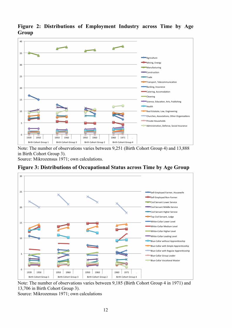
versus the Pre-Oil Crisis Post-War Period Figures 2 and 3 show the distributions of employment industry and occupational

status for the age groups 35–40 and 46–50 between 1939 and 1960 (birth cohort Groups 1

and 3) and the age groups 41–45 and 51–56 between 1950 and 1971 (birth cohort Groups 2

and 4). They thus clearly illustrate the distributional changes for prime-aged workers of

different birth cohorts within about a 10-year period, beginning immediately before WWII

and ending in 1950, 5 years after the war. The other decades considered, 1950–1960 and

1960–1971 represent post-war reconstruction up to the first oil crisis.

It is immediately obvious from Figure 2 that nothing spectacular happened to the

employment industry distributions for the defined birth cohort groups between 1939 and

1950, although manufacturing employment declined slightly between 1939 (WWII) and 1950

(early reconstruction). According to a difference-in-differences estimate, however, this

decline, from 35 to 34 percent for birth cohort Group 1, equals only about 2 percentage

points. Moreover, during subsequent decades (i.e., for birth cohort Groups 2 to 4), it

increased by about the same amount (one percentage point). This pattern is mirrored by a

similar change in the share of construction employment, which was positive between 1939

5

and 1950 but negative in the subsequent decades. Given the dramatic events in Europe during

WWII, these changes in employment structure seem small.4

One interesting observation that supports the claim of considerable continuity is the

constant share of employment in the “Administration, Defense, Social Insurance” category,

which shows virtually no decrease between 1939 and 1950. This finding suggests that, with a

few exceptions at the top (and apart from cohort turnover), the personnel of the

administration of the Third Reich were still in place in 1950.5 It is also significant that these

data refer to the same individuals asked about their jobs in 1939 and 1950. In fact, between

1950 and 1960, employment in this sector expanded because of a build-up of the welfare

state and, to a lesser extent for the cohorts considered here, the re-creation in 1955 of a West

German army.

The employment distributions by occupational status (see Figure 3) also reflect the

comparative smoothness of changes in the German labor market from 1939 to 1971: not one

element of the 1939–1950 period stands out as having a particularly high level of change.

One notable feature is the discernible increase (2 percentage points) in the share of non-

farming self-employed workers in contrast to the roughly equivalent decrease in the share of

workers with regular apprenticeships. A similar development is observable for birth cohort

Group 2 during the 1950–1960 period, although the increase in non-farming self-employment

is not quite as pronounced.

To represent the relations between employment industry (and occupational status) at

the beginning and end of each decade, I use two alternative measures of association (Agresti,

1984, p. 23f.; Freund and Wilson, 1997, p. 578): Pearson’s contingency coefficient

P = χ 2

n+ χ 2

and Cramér’s V

V = χ 2

n k −1( ) .

4 Another development, the comparatively strong decline in agriculture, seems to be a long-

term trend because it is observed for the entire1939–1971 period. 5 For example, Ludwig Erhard, who is regarded as the architect of the post-war Economic

Miracle, was already working on post-war economic planning at the end of 1942 (Ritschl, 2005; http://de.wikipedia.org/wiki/Ludwig_Erhard).

6

where χ2 is the χ

2 -statistic of the χ2 independence test and only valid if the number of

expected observations in each cell is at least 5. To ensure this latter, I reduce the number of

employment industry/occupational status categories from 15 to 10.

Tables 2 and 3 report the measures of association for employment industry and

occupational status, respectively. Table A1 (Table A2) in the Appendix shows the

distributions of employment industry in 1950 (1960) given employment industry in 1939

(1950). The measures of association in Tables 2 and 3 are based on the corresponding

absolute numbers in the cells of cross tables like Tables A1 and A2. Here only men are

included in the samples, but the results for men and women combined are almost numerically

identical, as shown in Tables A3 and A4 in the Appendix. I consider all workers first (the left

panels of the tables) before restricting the sample to German refugee workers, defined as

persons who lived in Central and Eastern Europe, including Eastern Germany, in 1939 (the

right panels of the tables). Although the Pearson’s contingency coefficient is generally larger

than Cramér’s V, the empirical results from both associational measures point to a similarly

large degree of stability for both employment industry and occupational status for all birth

cohorts in all three decades: 1939 to 1950, which covers WWII, 1950 to 1960, the first

decade of the Economic Miracle, and 1960 to 1971, the last decade before the oil crises

began. Nor does the Pearson’s contingency coefficient vary much between variables, time

periods, or birth cohorts, falling always between 0.91 and 0.93. Cramér’s V, on the other

hand, is more variable, but it too fails to show a lower degree of association in German

workers’ employment industry and occupational status between the 1939–1950 period and

later periods (1950–1960 or 1960–1971). Such a lower association would be expected if the

war had in fact altered careers in the German labor market considerably. Instead, although

somewhat smaller for the 1939–1950 period (the period covering WWII and early

reconstruction) than for the post-war periods, Cramér’s V is still of similar magnitude (0.76

versus 0.83, 078, and 0.80 in the shaded fields of Table 3, for example). For German refugee

workers, who by definition left their 1939 residence, the measures of association are

generally smaller, especially during the period covering WWII (1939-1950), but also for the

post-war periods (0.61 versus 0.71, 0.68, and 0.78 in the shaded fields of Table 3, for

example). Although it may be unsurprising that refugee German workers exhibit lower

measures of association than the average German worker, it is interesting to see that they

remain more mobile even in the post-war periods. This finding echoes similar results for

Finnish workers who left the territory that was transferred from Finland’s to the Soviet

Union’s rule after WWII (Sarvimäki, Uusitalo, and Jäntti, 2009).

7

4 Conclusions The overall finding of relatively stable employment by industry and occupational

status despite the WWII experience is interesting both historically and for its relevance to

today’s revolutions or military interventions. Historically, the observation that most German

workers retained the same employment industry and occupational status before and after the

war, with any changes differing little from corresponding dynamics during peace time, can

help explain the Economic Miracle (Wirtschaftswunder) in post-war Germany. It also

complements other studies that stress elements of continuity in Germany despite the war,

including Hirshleifer (1963), who emphasizes that only about 20 percent of industrial

capacity was destroyed, and Ritschl (2005), who identifies elements of continuity in the

regulatory economic framework of the mid-1930s and post-war period in Germany.

The finding is also relevant for the political and military interventions currently

occurring in other countries, especially in light of frequent allusions (e.g., during the Iraq

war) to Germany as a role model that transited from dictatorship to a democratic market

economy. It should be borne in mind, however, that this seemingly enormous political

transition occurred with a high degree of continuity not only in the allocation of labor but

also along other dimensions, such as laws pertaining to the economy. Hence, recent and

future regimes, such as those generated by the Arab Spring, might want to consider carefully

which parts of their economy and administration to build from scratch and which (select

elements) to exchange.

References

Absolon, R., 1960. Wehrgesetz und Wehrdienst 1935–1945, Das Personalwesen in der Wehrmacht [Military Law and Military Service: The Personnel Matters of the German Military 1935–1945], Harald Bold Verlag, Boppard am Rhein.

Agresti, A., 1984. Analysis of Ordinal Categorical Data, John Wiley & Sons, New York.

Aly, G., 2011. Hitlers Volksstaat, Raub, Rassenkrieg und nationaler Sozialismus, 2. Auflage, Fischer Taschenbuch Verlag, Frankfurt a.M. [first edition available in English as: Aly, G., 2007. Hitler’s Beneficiaries, How the Nazis Bought the German People, Verso].

Brakman, S., Garretsen, H., and Schramm, M. 2004. The Strategic Bombing of German Cities During World War II and Its Impact on City Growth, Journal of Economic Geography 4, 201–218.

8

Davis, D.R., and Weinstein, D.E. 2002. Bones, Bombs, and Break Points: The Geography of Economic Activity, American Economic Review 92, 1269–1289.

Freund, R.J., and Wilson, W.J. 1997. Statistical Methods, Revised Edition, Academic Press, San Diego, CA.

Hirshleifer, J., 1963. Disaster and Recovery: A Historical Survey, Memorandum RM–3079–PR, prepared for the United States Air Force Project, RAND.

Ichino, A., and Winter-Ebmer, R. 2004. The Long-Run Educational Cost of World War II, Journal of Labor Economics 22, 57–86.

Miguel, E., and Roland, G. 2011. The Long-run Impact of Bombing of Vietnam, Journal of Development Economics 96, 1–15.

Ritschl, A., 2005. Der späte Fluch des Dritten Reichs: Pfadabhängigkeiten in der Entstehung der bundesdeutschen Wirtschaftsordnung [The Late Curse of the Third Reich: Path Dependence in the Formation of the Economic System of the Federal Republic of Germany], Perspektiven der Wirtschaftspolitik 6, 151–170.

Särvimäki, M., Uusitalo, R. and M. Jäntti (2009). Long-Term Effects of Forced Migration, IZA Discussion Paper No. 4003, Bonn.

Schmölders, G. 1942. Der Wettbewerb als Mittel volkswirtschaftlicher Leistungssteigerung und Leistungsauslese [Competition as a Means to Economic Performance Increase and to Performance-Based Selection], Duncker & Humblot, Berlin.

Schmölders, G. 1943. Steuerumbau als Aufgabe für heute [Reorganization of Taxation as a Task for Today], Finanzarchiv 9, 246–272.

Waldinger, F., 2010. Quality Matters: The Expulsion of Professors and the Consequences for the PhD Student Outcomes in Nazi Germany, Journal of Political Economy 118, 787–831.

Waldinger, F., 2012. Bombs, Brains, and Science, The Role of Human and Physical Capital for the Creation of Scientific Knowledge, paper presented at the Society of Labor Economists (SOLE) Annual Meetings, Chicago, May 2012.

9

Table 1: Birth Cohort Groups by Age

Birth Year Age 1939 Age 1950 Age 1960 Age 1971 Birth Cohort

Group 1900 39 50 60 71 1 1901 38 49 59 70 1 1902 37 48 58 69 1 1903 36 47 57 68 1 1904 35 46 56 67 1 1905 34 45 55 66 2 1906 33 44 54 65 2 1907 32 43 53 64 2 1908 31 42 52 63 2 1909 30 41 51 62 3 1910 29 40 50 61 3 1911 28 39 49 60 3 1912 27 38 48 59 3 1913 26 37 47 58 3 1914 25 36 46 57 3 1915 24 35 45 56 4 1916 23 34 44 55 4 1917 22 33 43 54 4 1918 21 32 42 53 4 1919 20 31 41 52 4

Note: The shadings in the tables highlight the age correspondences between birth cohort groups 1 and 3 and 2 and 4, respectively.

10

Table 2: Measures of Association: Employment Industry–Men

Age Group/ Time Period

All Workers

German Refugee Workers

1939-1950

1950-1960

1960-1971

1939-1950

1950-1960

1960-1971

Pearson’s Contingency Index Birth Cohort Group 1 (Born 1900/04) 0.92

0.88

Birth Cohort Group 2 (Born 1905/09) 0.91 0.92

0.88 0.91 Birth Cohort Group 3 (Born 1910/14)

0.92

0.91

Birth Cohort Group 4 (Born 1915/19)

0.91 0.91 0.90 0.90 Cramér’s V

Birth Cohort Group 1 (Born 1900/04) 0.78 0.61 Birth Cohort Group 2 (Born 1905/09) 0.73 0.83 0.61 0.73 Birth Cohort Group 3 (Born 1910/14) 0.81 0.73 Birth Cohort Group 4 (Born 1915/19) 0.76 0.73 0.68 0.70

Note: Measures of Association are calculated based on cross tabulations of employment industry for the same persons at the start and end years of the corresponding time interval. For all workers, sample sizes vary from 8,886 to 13,888, for German refugee workers, sample sizes vary from 2,158 to 3,210. Source: Mikrozensus 1971; retrospective person-level data; male workers only; own calculations.

Table 3: Measures of Association: Occupational Status–Men


All Workers


1939-1950

1950-1960

1960-1971

1939-1950

1950-1960

1960-1971


0.88



0.92

0.90


0.91 0.92 0.89 0.92 Cramér’s V


Note: Measures of Association are calculated based on cross tabulations of occupational status for the same persons at the start and end years of the corresponding time interval. For all workers, sample sizes vary from 8,699 to 13,706, for German refugee workers, sample sizes vary from 2,145 to 3,194. Source: Mikrozensus 1971; retrospective person-level data; male workers only; own calculations.

11

Figure 1: Logarithm of Real GDP of Germany, the United Kingdom, and the United States

Source: http://www.fgn.unisg.ch/eurmacro/macrodata/datamtrx.html, now http://www.eurmacro.unisg.ch/macrodata/datamtrx.html; retrieved in 2004.

12

Figure 2: Distributions of Employment Industry across Time by Age Group

Note: The number of observations varies between 9,251 (Birth Cohort Group 4) and 13,888 in Birth Cohort Group 3). Source: Mikrozensus 1971; own calculations.

Figure 3: Distributions of Occupational Status across Time by Age Group

Note: The number of observations varies between 9,185 (Birth Cohort Group 4 in 1971) and 13,706 in Birth Cohort Group 3). Source: Mikrozensus 1971; own calculations

1

App

endi

x T

able

A1:

Em

ploy

men

t Ind

ustr

y D

istr

ibut

ion

in 1

950

(Col

umn

Perc

enta

ges)

by

Em

ploy

men

t Ind

ustr

y in

193

9–M

en o

f B

irth

Coh

ort G

roup

1 (B

orn

in 1

900-

1904

)

19

39

1 2

3 4

5 6

7 8

9 10

11

12

13

14

15

A

ll

1950

1 A

gric

ultu

re

80

1 2

4 3

2 1

3 0

1 0

0 0

17

2 15

2 M

inin

g, E

nerg

y 1

89

2 2

1 0

3 1

1 0

0 0

0 0

1 7

3 Man

ufac

turi

ng

9 5

83

7 7

6 6

11

12

6 4

8 4

33

10

34

4 Con

stru

ctio

n 6

1 3

78

2 2

3 1

1 1

2 1

0 0

4 11

5 T

rade

1

1 2

1 77

1

5 6

1 2

3 4

1 0

4 7

6 Tra

nspo

rt, T

elec

omm

unic

atio

n 1

1 2

3 1

85

2 1

1 1

2 0

0 0

2 8

7 Ban

king

, Ins

uran

ce

0 0

0 0

1 0

76

1 0

0 0

0 6

0 1

1 8 C

ater

ing,

Acc

omm

odat

ion

0 0

0 0

0 0

0 68

0

0 0

0 0

0 1

1 9 C

lean

ing

0 0

0 0

0 0

1 1

78

1 1

0 0

0 0

1 10

Sci

ence

, Edu

catio

n, A

rts,

Publ

ishi

ng

0 0

1 0

0 0

0 1

1 84

1

0 0

0 2

3 11

Hea

lth

0 0

0 0

1 0

0 0

0 0

87

0 0

0 0

1 12

Rea

l Est

ate,

Law

, Eng

inee

ring

0

0 0

0 0

1 0

1 0

1 0

83

0 0

2 1

13 C

hurc

hes,

Ass

ocia

tions

, Oth

er

Org

anis

atio

ns

0 0

0 0

0 0

0 1

0 1

0 0

82

0 1

1

14 P

riva

te H

ouse

hold

s 0

0 0

0 0

0 0

0 0

0 0

0 0

50

0 0

15 A

dmin

istr

atio

n, D

efen

se, S

ocia

l Ins

uran

ce

2 2

4 3

6 3

4 5

3 3

1 4

6 0

71

10

Su

m o

f Col

umn

Perc

enta

ges

100

100

100

100

100

100

100

100

100

100

100

100

100

100

100

100

Not

e: T

he e

ntrie

s in

the

tabl

e in

dica

te th

e pe

rcen

tage

of w

orke

rs w

ho w

orke

d in

indu

stry

“ro

w”

in 1

950

amon

g al

l wor

kers

who

wor

ked

in in

dust

ry

“col

umn”

in 1

939.

For

exa

mpl

e, th

e fir

st e

ntry

sta

tes

that

80

perc

ent o

f wor

kers

who

wor

ked

in a

gric

ultu

re in

193

9 w

ere

still

wor

king

in a

gric

ultu

re

in 1

950.

The

tabl

e is

bas

ed o

n 11

,264

obs

erva

tions

. So

urce

: Mik

roze

nsus

197

1; re

trosp

ectiv

e pe

rson

-leve

l dat

a; m

ale

wor

kers

onl

y; o

wn

calc

ulat

ions

.

2

Tab

le A

2: E

mpl

oym

ent I

ndus

try

Dis

trib

utio

n in

196

0 (C

olum

n Pe

rcen

tage

s) b

y E

mpl

oym

ent I

ndus

try

in 1

950–

Men

of

Bir

th C

ohor

t Gro

up 3

(Bor

n in

191

0-19

14)

19

50

1 2

3 4

5 6

7 8

9 10

11

12

13

14

15

A

ll

1960

1 Agr

icul

ture

77

1

1 1

1 0

0 0

0 0

0 0

0 0

0 9

2 Min

ing,

Ene

rgy

1 85

1

1 0

0 0

0 1

0 0

1 0

0 1

5 3 M

anuf

actu

ring

10

6

87

12

9 5

3 10

6

5 4

6 4

0 7

36

4 Con

stru

ctio

n 6

2 2

75

2 1

0 0

1 1

0 1

0 0

1 10

5 T

rade

1

0 3

1 77

1

2 3

1 2

2 2

2 0

1 8

6 Tra

nspo

rt, T

elec

omm

unic

atio

n 1

1 2

3 2

89

1 1

1 1

0 1

2 13

2

10

7 Ban

king

, Ins

uran

ce

0 0

0 0

2 0

89

1 0

1 0

0 0

0 1

2 8 C

ater

ing,

Acc

omm

odat

ion

0 0

0 0

1 0

0 82

1

1 0

1 2

0 0

1 9 C

lean

ing

0 0

0 0

0 0

0 0

86

0 0

1 0

0 0

1 10

Sci

ence

, Edu

catio

n, A

rts,

Publ

ishi

ng

0 0

0 0

1 0

1 0

0 86

0

2 3

0 1

2 11

Hea

lth

0 0

0 0

0 0

0 0

0 0

89

0 0

13

0 2

12 R

eal E

stat

e, L

aw, E

ngin

eeri

ng

0 0

0 0

0 0

1 0

1 0

0 79

1

0 1

1 13

Chu

rche

s, A

ssoc

iatio

ns, O

ther

O

rgan

isat

ions

0

0 0

0 0

0 0

0 1

1 0

1 87

0

0 1

14 P

riva

te H

ouse

hold

s 0

0 0

0 0

0 0

0 0

0 0

0 0

63

0 0

15 A

dmin

istr

atio

n, D

efen

se, S

ocia

l Ins

uran

ce

2 3

3 4

5 2

4 4

2 3

4 5

1 13

84

11

S

um o

f Col

umn

Perc

enta

ges

100

100

100

100

100

100

100

100

100

100

100

100

100

100

100

100

Not

e: T

he e

ntrie

s in

the

tabl

e in

dica

te th

e pe

rcen

tage

of w

orke

rs w

ho w

orke

d in

indu

stry

“ro

w”

in 1

960

amon

g al

l wor

kers

who

wor

ked

in in

dust

ry

“col

umn”

in 1

950.

For

exa

mpl

e, th

e fir

st e

ntry

sta

tes

that

77

perc

ent o

f wor

kers

who

wor

ked

in a

gric

ultu

re in

195

0 w

ere

still

wor

king

in a

gric

ultu

re

in 1

960.

The

tabl

e is

bas

ed o

n 13

,888

obs

erva

tions

. So

urce

: Mik

roze

nsus

197

1; re

trosp

ectiv

e pe

rson

-leve

l dat

a; m

ale

wor

kers

onl

y; o

wn

calc

ulat

ions

.

18

Table A3: Measures of Association: Employment Industry–Men and Women


All Workers


1939-1950

1950-1960

1960-1971

1939-1950

1950-1960

1960-1971


0.88



0.93

0.91


0.92 0.91 0.89 0.90 Cramér’s V


Note: Measures of Association are calculated based on cross tabulations of employment industry for the same persons at the start and end years of the corresponding time interval. For all workers, sample sizes vary from 13,046 to 19,901, for German refugee workers, sample sizes vary from 3,016 to 4,430. Source: Mikrozensus 1971; retrospective person-level data; own calculations.

Table A4: Measures of Association: Occupational Status–Men and Women


All Workers


1939-1950

1950-1960

1960-1971

1939-1950

1950-1960

1960-1971


0.88



0.92

0.90


0.91 0.92 0.90 0.92 Cramér’s V


Note: Measures of Association are calculated based on cross tabulations of occupational status for the same persons at the start and end years of the corresponding time interval. For all workers, sample sizes vary from 11,823 to 18,194, for German refugee workers, sample sizes vary from 2,973 to 4,305. Source: Mikrozensus 1971; retrospective person-level data; own calculations.

Documents

Employment Industry and Occupational Continuity in …ftp.iza.org/dp8372.pdf · Employment Industry and Occupational Continuity in Germany: ... Miracle (Wirtschaftswunder). This comparison