IZA DP No. 3688

Employment and Wage Effects of Privatization:Evidence from Hungary, Romania, Russia, andUkraine

J. David BrownJohn S. EarleÁlmos Telegdy

DI

SC

US

SI

ON

PA

PE

R S

ER

IE

S

Forschungsinstitutzur Zukunft der ArbeitInstitute for the Studyof Labor

September 2008

Employment and Wage Effects of

Privatization: Evidence from Hungary, Romania, Russia, and Ukraine

J. David Brown Heriot-Watt University

and IZA

John S. Earle Upjohn Institute for Employment Research,

CEU and IZA

Álmos Telegdy CEU, Hungarian Academy of Sciences

and IZA

Discussion Paper No. 3688 September 2008

IZA

P.O. Box 7240 53072 Bonn

Germany

Phone: +49-228-3894-0 Fax: +49-228-3894-180

E-mail: iza@iza.org

Any opinions expressed here are those of the author(s) and not those of IZA. Research published in this series may include views on policy, but the institute itself takes no institutional policy positions. The Institute for the Study of Labor (IZA) in Bonn is a local and virtual international research center and a place of communication between science, politics and business. IZA is an independent nonprofit organization supported by Deutsche Post World Net. The center is associated with the University of Bonn and offers a stimulating research environment through its international network, workshops and conferences, data service, project support, research visits and doctoral program. IZA engages in (i) original and internationally competitive research in all fields of labor economics, (ii) development of policy concepts, and (iii) dissemination of research results and concepts to the interested public. IZA Discussion Papers often represent preliminary work and are circulated to encourage discussion. Citation of such a paper should account for its provisional character. A revised version may be available directly from the author.

IZA Discussion Paper No. 3688 September 2008

ABSTRACT

Employment and Wage Effects of Privatization: Evidence from Hungary, Romania, Russia, and Ukraine*

We use longitudinal methods and universal panel data on 30,000 initially state-owned manufacturing firms in four transition economies to estimate the impacts of privatization on employment and wages. The results in all four countries consistently reject job losses and they never imply large wage cuts from privatization to either foreign or domestic owners. The domestic privatization estimates are close to zero for employment, while for wages they are negative but small in magnitude; estimated foreign privatization effects are nearly always positive and sometimes large for both outcome variables. We find that the negligible consequences of domestic privatization result from effects on scale, productivity, and costs that are large but offsetting in Hungary and Romania, and from small effects of all types in Russia and Ukraine. The positive employment outcome of foreign ownership results from a substantial scale-expansion effect that dominates the productivity-improvement effect, and the positive wage outcome from productivity improvement dominating the cost-reduction effect. JEL Classification: D21, G34, J23, J31, L33, P31 Keywords: privatization, employment, wages, foreign ownership, Hungary, Romania,

Russia, Ukraine Corresponding author: J. David Brown Heriot-Watt University School of Management and Languages Edinburgh EH14 4AS United Kingdom E-mail: J.D.Brown@hw.ac.uk

* This research was supported by the National Council for East European and Eurasian Research. We thank Joanne Lowery for editorial assistance, Philipp Jonas, Gábor Kézdi, and Mark Schaffer for econometric help and advice, and Tom Coupé, Vladimir Gimpelson, Rostislav Kapeliushnikov, and participants at presentations at the Upjohn Institute, Central European University, EERC-Kiev, Center for Labor Studies at the Higher School of Economics, University of Maryland, CUNY Graduate Center, CAED, SOLE, and AEA meetings for helpful comments. Assembling and preparing the data for this project involved large teams of collaborators, and we are grateful for conscientious work by Anna Horváth, Anna Lovász, Béla Személy, and Ágnes Törőcsik on the Hungarian data; Ioana Dan, Victor Kaznovsky, Catalin Pauna, Irina Vantu, and Ruxandra Visan on the Romanian data; and Natalia Akhmina, Tatiana Andreyeva, Serhiy Biletsky, Ivan Maryanchyk, Alexander Scherbakov, and Vladimir Vakhitov on the Ukrainian data. We are also grateful to the Hungarian National Bank for cooperation and data support on the Hungarian analysis, and to EROC (Economic Research and Outreach Center at the Kyiv-Mohyla School of Economics) for support of Ukrainian data collection and preparation.

1. Introduction An extensive theoretical and empirical literature has examined the effects of privatization

on firm performance. The theoretical papers describe mechanisms and conditions under which the performance effect may be positive, and the empirical studies attempt to estimate the magnitude of the effect for a variety of performance measures, with a particular focus on productivity. Most studies do find a positive effect, although it may vary across countries, measures, specifications, and new types of owners. In a comprehensive survey of research in the 1990s on privatization and performance, for instance, Megginson and Netter (2001) conclude that privatized firms “almost always become more efficient” (p. 381). In a meta-analysis of studies in transition economies, Djankov and Murrell (2002) conclude that “privatization is strongly associated with more enterprise restructuring...[but] statistically insignificant in the Commonwealth of Independent States (CIS)” (p. 740). More recently, Brown et al. (2006), using longer panel data than were available to previous researchers, find strongly positive effects of privatization on productivity in Hungary and Romania, a weak positive effect in Ukraine, and a slight negative effect in Russia; in all four countries, the effects of privatization to foreign investors are positive and larger than privatization to domestic owners.

Do the firm performance gains from privatization come at the expense of the jobs and earnings of employees? And in cases when privatization fails to improve performance are employment and wages of workers less likely to suffer, while more successful privatization implies bigger employment and wage declines? Many workers and policymakers seem to believe so.1 And many economists seem to agree: standard economic models of privatization imply that effective new owners raise productivity and lower costs, leading to job losses and wage cuts for workers.2 The tradeoff may be intuitive, but does it correspond with systematic empirical observation?

Our paper addresses these questions. Contrary to conventional views, we argue that the employment and wage effects of privatization are theoretically ambiguous, depending on underlying effects on productivity, scale, and cost efficiency that may work in opposing directions. An implicit assumption in the standard models, for example, is that output remains constant after privatization, in which case an increase in labor productivity necessarily implies a fall in employment. But if lower costs lead to an increase in quantity demanded or if the new owners are more entrepreneurial in expanding and entering markets (Frydman et al., 1999), then output may rise. This scale effect tends to increase employment, thus offsetting the productivity effect, and if the former dominates, the net result would be an employment rise. Similarly, the effect of privatization on wages may be negative if new private owners expropriate worker rents, as in hostile takeovers (Shleifer and Summers, 1988; Gokhale, Groshen, and Neumark, 1995). But the cost-reduction effect may be smaller if privatized firms pay more to attract new workers, elicit more effort, or share higher rents; in general, productivity improvements imply higher

1 Workers’ fears of privatization are well-documented through surveys in the UK (Nelson, Cooper, and Jackson, 1995), Poland (Rożnowski, Jochnowicz, and Marczuk 2003), and the US (Fernandez and Smith, 2005). López-de-Silanes, Shleifer, and Vishny (1997, p. 53) argue that public sector employees expect privatization “will lead to lower wages and loss of employment.” Druk-Gal and Yaari (2006) provide examples of employee opposition from Costa Rica, Egypt, Nicaragua, and Panama. Concerning policymakers, Megginson (2005, p. 389) writes that “all governments fear lay-offs resulting from privatization,” and Kay and Thompson (1986, p. 19) note that a possible goal of privatization could be “disciplining the power of public sector trade unions.” 2 See Vickers and Yarrow (1991), Boycko, Shleifer, and Vishny (1996), and Aghion and Blanchard (1998). For recent statements, see Kornai (2008): “If unemployment is rife...[t]his may mean putting off or slowing down a privatization where the new owner would immediately dismiss much of the work force” (p. 168); and, in a discussion of layoffs (p. 169): “Privatization serves first of all to enhance economic efficiency. But that has political and ethical implications which may come into conflict with the efficiency criteria.”

1

wages for given unit labor costs. Depending on the relative strength of these mechanisms, wages may either rise or fall as a result of privatization.

Not only does theoretical analysis fail to provide definitive predictions on the employment and wage effects of privatization, but also the existing empirical evidence is limited.3 Research has been hampered by small sample sizes, short time series, and difficulties in defining a comparison group of firms – limitations that both reduce the generality of the results and constrain the use of methods to account for selection bias in the privatization process. For example, in the first systematic study of the effects of privatization on employment and wages (albeit one with a focus as much theoretical as empirical), Haskel and Szymanski (1993) analyze 14 British publicly owned companies, of which four were privatized and the others were deregulated. Bhaskar and Khan (1995) use data for 2 years to estimate employment effects in 62 Bangladeshi jute mills, half of which were privatized. La Porta and López-de-Silanes (1999) analyze 170 privatized firms in Mexico, with post-privatization information limited to a single year.4 Other studies have sometimes included employment as one of several indicators of firm performance, but not the focus of analysis.5 Overall, the results from this small body of previous research are inconclusive, containing both negative and positive estimates.

In this paper, we report our empirical analysis of the effects of privatization on manufacturing firm employment and wages in Hungary, Romania, Russia, and Ukraine. These four countries span the range of approaches to privatization methods and reform experiences among transition economies, with Hungary considered one of the most successful, Russia and Ukraine among the least successful, and Romania in the middle.6 The data contain comparable annual information on relevant variables, particularly ownership data allowing us to distinguish state, domestic private, and foreign ownership types in each year. The variation in privatization methods and ownership structures permits an assessment of the tradeoff between the performance outcomes for firms and the wage and employment prospects for workers.

The coverage of the data is quite comprehensive, including nearly the universe of manufacturing firms inherited from central planning, both those eventually privatized and those remaining under state ownership in each country. The time series runs from the Communist and immediate post-Communist period, when all the firms were state-owned, through 2005 or 2006, well after most had been privatized. Unfortunately, the data do not contain measures of other potential outcomes, such as worker turnover and composition. A complete welfare analysis is therefore not possible, but the data are well suited for investigating the effects of privatization on a firm’s employment and average wage, essential issues in such an evaluation.

Our basic aim is to provide consistent estimates of these effects using much larger samples and longer panels than were available in earlier studies. The data provide comparison groups of state-owned firms operating in the same industries as those privatized, and the long

3 According to Megginson and Netter (2001, p. 381), “The question of whether privatization generally costs at least some SOE workers their jobs is still unresolved.” Anticipating part of our approach in this paper, they go on to suggest that “[t]he answer is ultimately based on whether sales increase faster than productivity in privatized firms.” 4 López-de-Silanes and Chong (2003) summarize the results from several studies of privatization in some Latin American countries. Kikeri (1998) and Birdsall and Nellis (2003) survey a number of case studies and small sample surveys of privatization and labor in several developing economies. Chong and López-de-Silanes (2002) study pre-privatization retrenchment programs. 5 Studies of firm performance with employment estimates include Megginson, Nash, and van Randenborgh (1994), Boubakri and Cosset (1998), D’Souza and Megginson (1999), Frydman et al. (1999), Claessens and Djankov (2002), and Lizal and Svejnar (2002); two of these find a positive effect of privatization on employment, three no effect, and one a negative effect. 6 The World Bank’s (1996) four-group classification of 26 transition economies, for example, puts Hungary in the first group of leading reformers, Romania in the second, Russia in the third, and Ukraine in the last. Similarly, the EBRD’s annual indicators of “progress in transition” invariably place Hungary at or close to the top of all transition economies; according to overall “institutional performance” in EBRD (2000), Hungary is ranked first, with a score of 3.5, while Romania is awarded 2.3, Russia 1.9, and Ukraine 2.1.

2

time series permit us to apply econometric methods developed for dealing with selection bias in labor market program evaluations. We consider a variety of specification and estimation approaches, including OLS, firm fixed effects, difference-in-difference matching, and random trend models. The last of these control not only for fixed differences across firms but also differing trend growth rates that may affect the probability of privatization and whether the new owners are domestic or foreign investors. We compare alternative estimators by examining the conditional difference in the dependent variable in the pre-privatization period.

We find no evidence of large negative impacts of privatization on either employment or wages. The domestic employment effects are rarely both negative and statistically significant, while for the wage rate they are negative but small in magnitude (-2 to -7 percent). By contrast, the estimated coefficients on foreign ownership are nearly always positive and frequently large for both dependent variables in all countries. These results are robust not only to choice of econometric specification but also to inclusion of exiting firms and to simple controls for spillovers. The dynamics of employment and wages around the privatization date reveal only minor fluctuations in event time, implying that preprivatization restructuring and spillovers to the state sector were insubstantial in these economies.

Therefore, while the data provide evidence of positive impacts of foreign privatization on employment and wages, the results for domestic privatization imply little changes in these variables, relative to the state-owned comparison group. Does the lack of domestic effects imply that this form of privatization makes little difference for firm behavior? To examine this question, we return to the underlying productivity, scale, and cost mechanisms. We decompose the estimated employment impact into a productivity-improvement effect that tends to lower employment (for given output) and a scale-expansion effect that tends to raise it (holding productivity constant); and we decompose the wage impact of privatization into cost-reduction and productivity-improvement effects, with expected negative and positive signs, respectively. The results imply that domestic privatization produces gains in both scale and productivity that offset each other in their employment outcomes, and it produces cost reductions and productivity improvements that have offsetting effects on wages. In Hungary and Romania, the scale, cost, and productivity effects of domestic privatization have all been large, while in Russia and Ukraine they have all been small. In all four countries, foreign privatization has resulted in still much larger scale, productivity, and cost effects, but the scale effects dominate the productivity effects, which in turn dominate the cost effects, resulting in the increased relative employment and wages in foreign firms that we observe after privatization.

The next section describes our data for each of the four countries, and Section 3 discusses their privatization programs. Section 4 explains the estimation procedures, and Section 5 presents the results. Conclusions are summarized in Section 6.

2. Data Our analysis draws upon annual unbalanced panel data for most of the manufacturing firms inherited from the socialist period in each of the four countries we study.7 The sources and variables are quite similar across countries. The State Committees for Statistics in Russia and Ukraine (Goskomstat in Russia and Derzhkomstat in Ukraine) are the successors to the branches

7 The data are similar to those in Brown et al. (2006), except for some earlier years in Russia, when the wage variable is unavailable, and the later period in all countries, when we have extended the time series for several additional years, as we describe below. We have also used additional information to recode the ownership variables and to repair some broken longitudinal links. Despite these differences, our results for productivity in this paper are quite similar to those reported by Brown et al. (2006).

3

of the corresponding Soviet State Committee. They compile the basic databases for our analysis in these countries, the annual industrial enterprise registries. These are supplemented by joint venture registries that are available in Russia and a database from the State Property Committee in Ukraine, which we have linked across years. The industrial registries are supposed to include all industrial firms with more than 100 employees plus those that are more than 25 percent owned by the state and/or by legal entities themselves included in the registry. In fact, the practice seems to be that once firms enter the registries, they continue to report even if the original conditions for inclusion are no longer satisfied. The data may therefore be taken as corresponding to the “old” sector of firms (and their successors) that were inherited from the Soviet system. Certainly with respect to this set of firms, the databases are quite comprehensive.

The Russian database includes the years 1985-2004 and 2006, and the Ukrainian database covers 1989 and 1992-2006. Russian wage data, however, are available only in 1989, 1992-2004, and 2006. Employment in Russia in all years and in Ukraine from 1989 to 1996 is defined as the average number of registered employees in industrial production divisions of the enterprise; this definition includes non-production and supervisory workers but excludes employees in “nonindustrial divisions.” Although information on the exact size of these divisions is scant, by all accounts they tend to be very small fractions of total firm employment. In Ukraine, the available employment variable includes employees in all divisions in the years 1997-2006. The wage variable in Russia in all years and in Ukraine for 1989 and 1992-1996 refers to the annual wage bill for registered employees of industrial divisions, including both monetary and in-kind accrued payments (the latter valued at “market prices”), divided by average employment. Wages are deflated by consumer price indices. The Hungarian and Romanian data tend to be more similar to each other than to those in the Soviet successor states. The basic data sources are the National Tax Authority in Hungary and the Ministry of Finance in Romania, which provide data for all legal entities engaged in double-sided bookkeeping. In addition, the Romanian data are supplemented by the National Institute for Statistics’ enterprise registry and the State Ownership Fund’s portfolio data. The Hungarian data are available for 1986-2005, the Romanian for 1992-2006. The employment definitions in both cases refer to average number of employees over a year, and wages are defined as the annual wage bill (including monetary and non-monetary benefits) for all employees divided by average employment and again deflated by consumer prices.

In order to make the samples comparable across countries, some truncation of the Hungarian and Romanian data was necessary. Firms are included if at first observation they operate in an industrial sector, because the Russian and Ukrainian data exclude non-industrial firms as well as industrial firms that were classified as non-industrial when they first appeared. In all four countries, the data are restricted to manufacturing (NACE 15-36) because some of the nonmanufacturing industrial sectors (chiefly mining) are defined noncomparably in the Russian and Ukrainian classification system (OKONKh).8 We include only “old” firms, those existing prior to 1992 (1990 in Hungary) or state-owned at first observation, because de novo firms are not at risk of privatization. In addition, privatized firms are included only if they are majority state in their first observation in the regressions, so that the base category consists exclusively of state firms.9

8 Recycling (NACE 37) is also excluded because of noncomparability with the OKONKh classification system. 9 In Russia and Ukraine, formal privatization started only after 1992, so firms in our data before this year must be state-owned. Romanian privatization was very gradual, starting with only a few firms in 1992 and 1993, so the state entry sample is little reduced by the lack of data in earlier years.

4

These data have been extensively cleaned to remove inconsistencies and to improve longitudinal linkages that may have been broken due to change of firm identifier from one year to the next (associated with reorganizations and changes of legal form, for instance). The inconsistencies were evaluated using information from multiple sources (including not only separate data providers, but also previous year information available in Romanian balance sheets and Russian and Ukrainian registries). Observations on variables showing highly volatile fluctuations were removed if they met any of the following criteria: increasing by a factor greater than five then declining by a factor greater than five, increasing by a factor greater than 10 in the year after entry, or decreasing by a factor of 10 in the final year of observation.10

Table 1 contains the numbers of observations for the employment and wage regressions by ownership and country.11 Numbers of observations for privatized firms are also shown for the pre- and post-privatization periods separately, and on both a total and average per-firm basis. We are able to study an average of 3.7 Hungarian, 5.8 Romanian, 6.8 Russian, and 4.7 Ukrainian observations per firm prior to domestic privatization in the employment regressions, and 7.4 Hungarian, 7.4 Romanian, 6.8 Russian, and 7.0 Ukrainian observations per firm are included post-domestic privatization. The total number of foreign privatizations is smaller, though the average number of observations per firm pre- and post-privatization are similar to domestic privatization. The number of observations for wages is only slightly smaller, except in Russia, where wages are unavailable in 1985-1988 and 1990-1991. Otherwise, missing values for particular variables do not reduce the sample much, and the unbalanced nature of the data is due rather to entry and exit. Table 2 provides summary statistics for employment and wages for the regression samples. The data imply that average employment for these manufacturing firms is substantial in each country. Average wages vary considerably across countries, being highest in Hungary and lowest in Ukraine. Two types of measurement error merit further discussion. The first concerns under-reporting of wages to avoid taxes and social security contributions. Our discussions with knowledgeable observers in these countries suggest that while under-reporting is common in small service sector firms, it is unlikely to be very serious in our samples of large manufacturers because of the difficulty of secretly paying many employees. The observers also indicate that to the extent wage under-reporting in these firms does occur, it is most likely to happen in those privatized to domestic owners; state-owned firms are subject to tight controls and have fewer incentives to avoid taxes, while foreign-owned firms are less likely to hide wages. This implies that our estimates of the wage effects of domestic privatization will be negatively biased, so that an estimated effect of zero (or slightly negative) might reflect a true effect that is positive. A second type of measurement error, especially in Russia and Ukraine, could arise from wage arrears. The wage variable in our data represents accrued obligations to employees, and systematic differences in arrears across ownership types could create biases relative to actually paid wage differentials. Arrears appear to be slighly lower in domestic privatized firms relative to state-owned enterprises (e.g., Earle and Sabirianova, 2002), resulting in relatively understated paid wages and thus a negative bias on estimates of the domestic wage premium. The limited evidence on foreign-owned employers suggests they have much lower arrears, implying that the estimated foreign wage effect would be still more negatively biased. We consider these and 10 These cleaning rules result in the loss of less than 0.3 percent of the observations of any regression sample, and they have negligible effects on the results. 11 The total number of firms and firm-year observations in the regression samples are shown in Table 4 and its notes. The precise definitions of domestic and foreign ownership in privatized firms are provided in the next section.

5

other sources of possible measurement error in discussing our results.

3. Privatization Policies and Their Implications The process of privatizing large enterprises took many years in most countries, and the

methods and tempos differed quite significantly across the four countries we study in this paper. Hungary got off to an early start in ownership transformation and maintained a consistent emphasis on case-by-case sales throughout the transition. At the very beginning, transactions tended to be “spontaneous,” initiated by managers, sometimes in combination with foreign or other investors (Voszka, 1993). From 1991, the sales process became more regularized, generally relying upon competitive tenders open to foreign participation, although management usually retained significant control. Unlike elsewhere, there were no significant preferences given to workers to acquire shares in their companies nor a mass distribution of shares aided by vouchers. Hungarian privatization thus resulted in very little worker ownership (involving only about 250 firms), very little dispersed ownership, and instead significant managerial ownership and highly concentrated blockholdings, many of them foreign (Frydman et al., 1993a). Although the process appeared at times to be slow and gradual, in fact it was completed earlier than in most other East European countries.

In Romania, by contrast, the early attempts to mimic voucher programs and to sell individual firms produced few results, and after a few “pilots” privatization began in earnest only in late 1993, first with the program of Management and Employee Buyouts, and secondly with the mass privatization of 1995-96 (Earle and Telegdy, 2002). The consequences of these programs were large-scale employee ownership and dispersed shareholding by the general population, with little foreign involvement. Beginning in 1997, foreign investors became more involved, and blocks of shares were sold to both foreigners and domestic entities. The result was a mixture of several types of ownership and a moderate speed compared to Hungary.

Russia and Ukraine’s earliest privatization experiences have some similarities to the “spontaneous” period in Hungary, as the central planning system dissolved in the late 1980s and decision-making power devolved to managers and work collectives (Frydman et al., 1993b). The provisions for leasing enterprise assets (with eventual buyout) represented the first organized transactions in 1990-1992, but the big impetus for most industrial enterprise privatization in Russia was the mass privatization from October 1992 to June 1994, when most shares were transferred primarily to managers and other employees who received large price discounts (Boycko, Shleifer, and Vishny, 1995). Some shares (generally 29 percent) were reserved for open voucher auctions, and these resulted in a variety of ownership structures, from dispersed outsiders holding shares through voucher investment funds to domestic investors acquiring significant blocks; but there were few cases of foreign investment. Blockholding and foreign ownership became more significant through later sales of blocks of shares and through secondary trading. Ukraine used somewhat different mechanisms but in general followed Russia’s pattern at a somewhat slower pace. In both countries, the initial consequence was large-scale ownership by insiders and some blockholding by domestic entities, while concentration and foreign ownership subsequently increased.

These general patterns are reflected in Table 3, which contains the percentage of firms privatized to domestic and foreign owners, based on our regression samples in each country.12

12 Ownership is measured at the end of each calendar year, and privatization is measured as a change in ownership type from the end of one year to the end of the next. We define a firm as private if more than 50 percent of the shares are privately held; it is domestic if it is private and more shares are held by domestic than by foreign owners; it is foreign if it is private but not domestic. Nearly all foreign

6

As of late 1992, 43.6 percent of the Hungarian firms had already been privatized, while privatization of the manufacturing firms in our database had not yet started in Romania, Russia, and Ukraine. By the end of the period, most firms had been privatized in all four countries, although enough state-owned firms remain in each country to serve as a comparison group in our estimations.13 The percentage of firms majority privatized to foreigners is by far the highest in Hungary, reaching nearly 17 percent of all entities by 2004. In Romania, the percentage reaches 6.7 percent, 1.2 percent in Russia, and 1.0 percent in Ukraine. Given our sample sizes, these are sufficient to estimate coefficients.14

The cross-country differences in privatization policy design could affect the extent of selection bias in the privatization process as well as the measured impact of privatization on employment and wages. Privatization through competitive sales (auctions or tender) to outside investors implies that the buyers fully assess the firm’s operating and financial performance as well as its potential for growth.15 Such thorough assessments are less common under giveaway privatization methods, where the buyer’s own capital is not put at risk. Privatization leading to highly dispersed ownership structures also provides little incentive for any single acquirer to gather such information. Relative to foreigners, domestic investors may have extra information on the extent of overstaffing and excessive wages, and thus the potential for restructuring. If these differences across firms tend to be fixed, then they will be removed by firm fixed effects, and if they tend to grow at a constant rate they will be removed by firm-specific trends.16

In predicting the consequences of alternative privatization methods, we consider the underlying productivity, cost, and scale mechanisms through which privatization may impact employment and wages. Worker-owners are likely to oppose wage cuts and labor-saving restructuring, and they are unlikely to have incentives or resources to expand. Outside blockholders should favor productivity improvement and cost reduction, and they are also more likely to respond to opportunities for expansion. Among outside owners, foreign investors with superior management skills, new technologies, knowledge of markets, and access to finance seem likely to be the most successful at raising productivity, scale, and cost efficiency. Outsiders with small shareholdings may also benefit from efficiency improvements and scale expansion, but they are less likely to influence the firm’s behavior. Therefore, the productivity, cost, and scale effects of privatization are likely to be smallest for domestic owners in countries where insider and mass privatization predominated, larger in cases where domestic outsiders acquired blocks of shares, and largest for privatization to foreign investors. Because these mechanisms tend to be offsetting, however, their net effects on employment and wages are a priori ambiguous. The next section describes our methods for estimating the effects empirically.

privatized firms by this definition are majority foreign-owned. The Russian data do not contain an ownership variable before 1993, nor do they provide percentage shareholding. But virtually all the privatizations in our data are mass privatizations, so the earliest they could take place was October 1992, and nearly all led to majority private ownership (see, e.g., Boycko, Shleifer, and Vishny, 1995). 13 We assume a single ownership change and recode cases of multiple switches to the modal category after the first change (ties are decided in favor of private and foreign). In Hungary there are 71 such cases, in Romania 15, Russia 2,918, and in Ukraine 6. Many Russian firms were reclassified as state in 2000 or 2001, when ownership codes changed; such mass renationalization did not occur, so our recoding corrects this problem. The nonmonotonicity of percent privatized in Table 4 is due to split-ups of state firms. 14 See Table 1 for sample sizes. The Russian registries contain codes for state, domestic, joint ventures, and 100 percent foreign firms, but foreign shares are available only for a subset of firms in four years. We classify all joint ventures as foreign, but the results are very similar if we include only those foreign firms with a majority foreign share in at least one of the four years. 15 For legal entities buying state-owned companies or assets, some assessments may be legally required as “due diligence.” 16 See Gupta, Ham, and Svejnar (2000) for a study of selection bias in privatization sequencing. Appendix A contains a brief analysis of the preprivatization characteristics of firms later privatized as possible indicators of selection bias in the privatization process.

7

4. Empirical Strategy We follow the broader literature on the effects of privatization in estimating reduced form

equations, while trying to account for heterogeneity and simultaneity bias (Djankov and Murrell, 2002; Megginson and Netter, 2001). A first potential estimation problem is the possibility of aggregate shocks correlated with employment, wages, and ownership. Studies that estimate a privatization effect as the difference between pre- and post-privatization levels for a sample of privatized firms (e.g., Megginson, Nash, and van Randenborgh, 1994) are unable to distinguish the effect of privatization from such aggregate fluctuations. Moreover, shocks may be industry-specific, and available deflators may not perfectly capture price changes. Most studies have too few observations at their disposal to be able to account for industry-specific fluctuations, yet if these are correlated with privatization, the estimates may be biased. Taking advantage of the large samples in our data, our regressions compare the performance of privatized firms with state-owned control firms in the same industry-years.17 Unlike most previous studies, these data contain firms that remain in state ownership throughout the period of observation.

A second estimation problem involves ambiguities in timing, both in the precise date of privatization (sometime in the year between observation dates) and in how long it takes for any effects to emerge. We address these issues by investigating the dynamics of the effect before and after the privatization year. Examining the immediate pre-privatization dynamics provides information on whether firms were restructuring in anticipation of ownership change.18 Examining the earlier pre-privatization dynamics is useful for assessing selection bias appearing as conditional differences in the dependent variable prior to ownership change. Finally, the dynamic specification sheds light on the possibility of general equilibrium effects resulting from labor market competition among employers. If foreign-owned firms tend to pay higher wages, for instance, then others may respond by raising their own wages in order to compete for workers, and our estimates of the foreign coefficient will be an understatement of the true effect. A complete general equilibrium analysis is beyond the scope of this paper, but if the spillovers are not instantaneous, they should be reflected in the dynamics of the effects: large initially but diminishing as domestic firms “catch up” to the foreign practice.19

Perhaps the most difficult problem is the possibility of selection bias in the privatization process. Politicians, employees, and investors may all influence whether a firm is privatized and whether the new owners are domestic or foreign. Politicians concerned with unemployment may prefer to retain firms with the worst prospects in state ownership in order to protect workers from layoffs and wage cuts, and employees themselves may try to prevent privatization in such cases. Potential owners are also likely to be most interested in purchasing firms with better prospects, and foreign investors may be better (or, conceivably, worse) at “cherry-picking.”

In principle, several alternative strategies could be employed to address selection bias. One is to use instrumental variables. As is commonly the case (but see Hanousek, Kocenda, and Svejnar, 2005), our data do not contain instruments that are both important determinants of the privatization choice and orthogonal to the error terms in the employment and wage equations. A 17 We use 2-digit NACE industries, combining food and beverages (15) with tobacco (16), coke, refined petroleum products and nuclear fuel (23) with basic chemicals (24), and office machinery and computers (30) with radio, television, and communications equipment and apparatus (32) due to small numbers of observations in sectors 16, 23, and 30 in some countries. 18 Aghion, Blanchard, and Burgess (1994) argue that anticipatory behavior is likely to be negative if the expectation of post-privatization loss of control – or of job – leads to increased asset stripping by managers; but Roland and Sekkat (2000) argue that good managers restructure their companies prior to privatization. La Porta and López-de-Silanes (1999) find negative anticipatory effects in their study of Mexico. 19 As a further check on possible spillover effects, in one specification we also control for the regional proportions of firms privatized to domestic and foreign owners, respectively. Variations in sectoral proportions are absorbed by the industry-year interaction dummies.

8

second approach is to include lagged dependent variables and estimate dynamic GMM models. But the need for a long lag structure precludes firms with few years of data, introducing sample selection bias, and it rules out tracing the dynamics of the privatization effects. Dynamic GMM model results can also be quite sensitive to small changes in specification where the dependent variables exhibit a high degree of persistence, the case with employment and wages.

A third strategy is to use a matching estimator that pairs each privatized firm with one always remaining state-owned, the most similar based on observable pre-privatization characteristics. To address remaining pre-privatization differences, matching can be combined with difference-in-differences in panel data (e.g., Arnold and Smarzynska Javorcik, 2005; Gong et al., 2006). A drawback is that the focus on differences between treated firms and never treated firms ignores potentially relevant information on firms to be treated sometime in the future. Our data contain thousands of observations for not-yet-privatized firms that could be useful – and likely more similar – controls for privatized firms in the same industry-years. With an unbalanced panel, additional problems arise from selection bias due to differences in time series lengths and exit rates. Requiring information from several years before privatization can severely restrict the sample, as many firms do not have long pre-privatization histories, but variables measured just before privatization may be contaminated by anticipatory effects. A matched sample is also affected by differential exit rates; if either the treated or matched untreated firm exits, the pair drops out of the regression in all subsequent years. If firms are matched within industries, it is possible that the privatized firm’s success causes the always state firm to exit, so pairs with particularly unequal post-treatment performance are most likely to disappear. This also implies that some important longer-run effects will not be captured.

Rather than matching each privatized firm to a single always state-owned firm, one could instead use all non-privatized firms in the same industry-year as the comparison group in a panel regression approach. Observations on privatized firms can contribute to identifying the estimates if at least one non-privatized firm remains in the same industry-year, reducing the exit bias problem.20 The panel regressions incorporate all available pre-privatization information when controlling for differences between the treated and non-treated groups, rather than imposing assumptions about particular years for matching. Important forms of selection bias can be handled with firm fixed effects (FE) for time-invariant differences, and by adding firm-specific trends (FE&FT) to control for the possibility of selection for privatization (or foreign versus domestic ownership) based on growth opportunities.21 The main drawback of using all available non-privatized firms in the industry-year as the comparison group relative to using only the matched never privatized (state-owned) firm is the possibility that the former control group may be less similar to the treated firm prior to treatment. On the other hand, firms just undergoing privatization may well be more similar to not yet privatized firms than to never privatized firms. To investigate the robustness of our results, we estimate the effects using each approach.

The panel regression model takes the following form for each country separately: yit = Djtγjt + wtαi + θitδ + uit, (1)

20 This bias may be large, because matching greatly reduces the post-privatization sample. For example, the average number of post-privatization domestic ownership observations per firm in the panel regressions for employment is 7.4 in Hungary, 7.4 in Romania, 6.8 in Russia, and 7.0 in Ukraine (see Table 2), while for nearest neighbor matching it is drastically reduced to 1.6 on average in Hungary, 4.2 in Romania, 4.6 in Russia, and 4.4 in Ukraine. The differences are similar for foreign ownership and for the wage samples. A complete set of numbers analogous to those in Table 2, but for the single-firm matched sample, is available upon request. 21 Though the inclusion of firm-specific trends has the advantage of controlling for pre-privatization trends, this may also capture some of the privatization effect, especially when most of a firm’s observations in the data are post-privatization.

9

where i indexes firms from 1 to N, j indexes industries from 1 to J, and t indexes time periods (years) from 1 to T.22 In alternative specifications, yit is the natural logarithm of the firm’s employment (e) and average wage rate per worker (w). Djt is a 1 x JT vector of industry-year interaction dummies; γjt is the associated JT x 1 vector of coefficients; and uit is an idiosyncratic error.23 The dimensions of the other terms in the equation vary across specifications: wt is a vector of aggregate time variables, αi is the vector of associated individual-specific slopes, θit is the vector of ownership measures, and δ are the ownership effects of interest in this paper. In the OLS regressions wt ≡ 0. In the FE regressions wt ≡ 1, so that αi ≡ αi is the unobserved effect. The FE&FT model specifies wt ≡ (1, t), so that αi ≡ (α1i, α2i), where α1i is a fixed unobserved effect and α2i is the random trend for firm i. In practice, the FE&FT model is estimated in two steps, the first detrending all variables for each firm separately and the second estimating the model on the detrended data.

We investigate two alternative specifications of the ownership variables θit. The simplest uses two post-program dummies, where θit ≡ (Domesticit-1, Foreignit-1), and δ ≡ (δd , δf ) are the parameters of interest.24 Foreignit-1 is defined = 1 if the firm is majority foreign owned at the end of the previous year, and Domesticit-1 = 1 if the firm is majority privately owned at the end of the previous year, but not majority foreign owned. The coefficients of interest (δd , δf) are then the mean within-country-industry-year difference in the dependent variable between domestic privatized firms and majority state-owned and between firms majority foreign and majority state-owned, respectively. We also estimate dynamic specifications, where dummy variables for the years before and after privatization are interacted with indicators for whether the firm is ever domestically privatized or foreign privatized. Designating τ as the index of event time, the number of years since privatization, so that τ < 0 in the pre-privatization years, τ = 0 in the year in which ownership change occurs, and τ > 0 in the post-privatization years, then θit ≡ (Domesticitτ, Foreignitτ), δ ≡ (δτd, δτf), and τ = -5-, -4, -3, -2, -1, 0, 1, 2, 3, 4, 5+, where -5- is five and more years before privatization, and 5+ is five and more years after privatization. The privatization year 0 is the omitted category in the regressions.

The matching method is implemented by first estimating a multinomial logit regression with three outcomes (remaining state, privatized to domestic owners, and privatized to foreign owners) as a function of log employment, squared log employment, log wage, squared log wage, log ratio of capital stock to employment, and multifactor productivity, all measured in the year prior to privatization, as well as 19 sector dummies and year dummies. 25 Log of employment in the year prior to privatization minus its value two years before privatization is also included to control for pre-privatization trends. The sample consists of privatized firms in the year of privatization and always state-owned (never privatized) firms in industry-year cells containing at least one privatization. Based on the propensity scores for the domestic and foreign privatization

22 J=19. T varies by country and dependent variable: 20 for Hungary, 15 for Romania, 20 for Russian employment, 14 for Russian wage, and 16 for Ukraine. 23 Our estimates permit general within-firm correlation of residuals using Arellano’s (1987) clustering method. The standard errors of all our test statistics are robust to both serial correlation and heteroskedasticity. 24 We infer privatization when a firm changes status from state to private between the end of one year and the next. This implies that the date the new owners acquire formal authority (e.g., the first post-privatization shareholders’ meeting) varies across firms, with some early in the final pre-privatization year. Some assumption on the first “post” year is necessary in this analysis, but as our estimates of the dynamics of the effect suggest, the results are not at all sensitive to this assumption. 25 Imbens (2000) suggests a multinomial regression in cases of multiple treatments. Our use of this method takes into account possible differences in the selection into domestic and foreign private ownership, and indeed we find significant differences between the coefficients explaining domestic versus foreign privatization in the multinomial logits. Multifactor productivity is the residual from an industry-specific Cobb-Douglas production function in capital and labor (using 19 sectors).

10

outcomes from this regression, we match each privatized firm to the nearest always state-owned firm in the same industry-year cell.26 We then estimate the following outcome regression: yit – ymt = αi + θitδ + uit, (2) where m denotes the matched control firm, and the other variables are defined as in equation (1). All available pre- and post-privatization observations for the matched pairs are included in these regressions. The inclusion of firm fixed effects removes time-invariant differences between the privatized firms and matched controls.

We use dynamic ownership specifications to implement specification tests that help determine the extent to which the alternative specifications deal with selection bias. Our method generalizes the Heckman and Hotz (1989) “pre-program test” of the conditional difference in the outcome for treated and control groups in one pre-treatment period. The assumption is that, once the test is satisfied, the only cause of differences between the two groups after treatment is the treatment itself. Using a similar dynamic specification of ownership effects as described above, but with five and more years before privatization as the omitted category, we carry out t tests of τ = -4, -3, and -2, as well as F tests for the joint significance of these dummies. Examining the t tests for several years addresses Heckman, LaLonde, and Smith’s (1999) concern about sensitivity to the choice of pre-treatment period. Studying each available pre-privatization year avoids this “alignment fallacy.” In addition to the pre-program test, we conduct F tests on the joint probability that all FEs = 0, and on the joint probability that all FTs = 0 in regressions with a single post-dummy for privatization. Finally, we conduct Hausman-type specification tests of the differences in the entire vector of coefficients resulting from adding FEs to the OLS specification, and from adding FTs to the FE specification.

To shed light on the economic mechanisms underlying the estimated impacts of privatization on employment and wages, we decompose each of these into two further effects: scale and productivity effects for employment, and productivity and cost effects for the wage. For the employment decomposition, we estimate versions of equation (1) where the dependent variables yit are the natural logarithms of output (x) and labor productivity (lp = x – e, with e = ln[employment]). The decomposition follows from the basic identity: e ≡ x – (x – e) ≡ x – lp. (3) Linearity of the estimators of the privatization effect with these dependent variables implies that the estimated coefficients can also be decomposed. We estimate the equations with consistent samples and the ownership specification θit ≡ (Domesticit-1, Foreignit-1), so that δ ≡ (δd , δf ). Thus δe = δx – δlp, where superscripts represent the dependent variable in each equation. We similarly decompose wage effects by estimating equations with the natural logarithm of unit labor cost (ulc = w + e - x) and productivity (lp), relying on the identity: w ≡ (w + e – x) + (x – e) ≡ ulc + lp. (4) The estimated wage effect of privatization is therefore equal to the unit labor cost effect plus the productivity effect: δw = δulc + δlp. Since the unit labor cost effect is expected to be negative, the cost and productivity effects may work in opposite directions on wages. In these regressions, FE and FE&FT models are estimated, and industry-year effects are included as controls.

The final estimation issue, which is relevant to all of these methods and all previous research on this topic, concerns the use of information only on reporting firms. A difficult problem is how to handle exit because, as discussed in Section 2, the permanent disappearance of

26 The matching is with replacement – i.e., a never privatized firm could potentially serve as the control firm for more than one privatized firm. If replacement were not allowed, many privatized firms could not be matched, as the data contain more firms that are privatized than never privatized, creating even worse sample selection problems.

11

a firm from the data may represent a genuine shutdown or merely a change in name or legal form. In the former case, it would be desirable to count these as job losses, while in the latter, it would not. Despite extensive cleaning of the longitudinal linkages, we can distinguish shut-downs from simple reregistrations only imperfectly. To assess the potential of exits to influence our results, however, we estimate specifications of equation (1) with the dependent variable transformed as the ratio to the firm average and set to zero in the first year after exit. We also estimate probit equations for exit as a function of ownership and industry and year dummies. The next section reports the results.

5. Results The results from estimating relation (1) by OLS, fixed firm effects (FE), and firm-

specific trends (FE&FT) are displayed in Table 4.27 The OLS estimates of the employment effects of domestic privatization illustrate the pitfalls of simple cross-sectional comparisons, with coefficients ranging widely from -0.49 in Hungary to +1.00 in Russia. Both of these become tiny and statistically insignificant when FE are added, while the Romanian estimate jumps to 0.16 and the Ukrainian falls to -0.06. The differences between OLS and FE estimates of the domestic wage effects are smaller, except for Russia with OLS and FE coefficients of 0.19 and -0.03, respectively. All FE estimates of the domestic wage coefficients are negative and statistically significant, but small in magnitude: 2-5 percent. The FE&FT estimate of domestic privatization on employment in Romania is insignificant, while the coefficient in Russia is larger and significant. The domestic wage effects remain negative, statistically significant, and small, Russia having the largest magnitude (-0.07). Thus, the domestic results generally imply effects close to zero for both dependent variables in all countries. The estimated wage impacts are small and negative, but there is some reason to believe that the wage coefficients may be negatively biased by measurement error, as we discuss shortly.28

By contrast with the generally small to negligible domestic results, the effects of privatization to foreign investors are estimated to be positive for both employment and wages in every country, with the exception of Romanian employment, where inclusion of firm-level trends generates a negative and insignificant coefficient. The magnitudes are usually large and highly statistically significant. The attenuation of the foreign results when including firm-specific trends could be due to the application of a less efficient estimator to a relatively small number of foreign observations. Nevertheless, these results do not suggest that foreign privatization has reduced employment or wages.

Because the matching approach has several disadvantages compared with these panel regressions and the findings are in any case qualitatively similar, we report the matching results in Appendices. Appendix B1 shows results using the single comparison firm matching approach, which implies effects quite similar to the FE results in Table 4. The main exceptions are the significantly larger domestic and foreign coefficients for Romanian employment, which appear to result from the fact that the matching approach uses only always state firms as the

27 The sample observations do not vary across specifications when adding FEs and FTs. Note, however, that once FEs are added, firms with a single observation no longer meaningfully contribute to the regression, and firms with one or two observations do not contribute to FE&FT regressions. To check whether this leads to sample bias, we have run separate OLS regressions without firms with single observations, and also ones without firms with one or two observations, as well as FE regressions without firms with one or two observations. The OLS coefficients move slightly downward, while the FE coefficients are virtually unaffected by the sample change. 28 Wage impacts of minus 2–7 percent are small relative to the fluctuations of wages in these countries during this period, and also compared with other types of effects estimated by economists. Standard estimates of the union relative wage effect, for example, generally lie in the range from 15 to 20 percent (e.g., Card’s (1996) estimates range from 0.14 to 0.21).

12

benchmark rather than also including pre-privatized firms.29 Appendix B2 shows results from single comparison firm matching where pre-privatization employment trends are omitted from the multinomial logit regression. There are differences compared to Appendix B1: the domestic privatization effect on employment becomes positive in Hungary, and the foreign coefficients in Ukraine become smaller, illustrating the sensitivity of point estimates to small changes in the matching method.30 All the methods nevertheless suggest the same general conclusions: domestic privatization effects are usually close to zero, and foreign privatization effects are nearly always positive, statistically significant, and large in magnitude.

To see how well each of these specifications handles selection bias, in the sense of observable differences in pre-privatization outcomes, we report variants of the Heckman-Hotz (1989) “pre-program test.” As shown in Appendix C, the OLS specifications result in large and highly statistically significant differences two to four years prior to either type of privatization compared to those five or more years before privatization, suggesting the presence of serious selection bias. Adding FEs significantly reduces the coefficients, but some substantial and statistically significant differences remain in some cases: Romanian pre-domestic and pre-foreign firms show clear positive trends, Russian and Ukrainian pre-domestic firms have negative employment trends, and Romanian pre-foreign and Russian pre-domestic and pre-foreign firms exhibit positive wage trends. The FE&FT specification removes each of these trends, with the only remaining visible pre-privatization trend a negative one in Hungarian pre-foreign employment. As discussed below, this trend sharply reverses in the year before privatization, however, suggesting that this should not pose a problem for estimating the privatization effect. The results corresponding to the matching specification in Appendix B1 show large, statistically significant domestic coefficients for employment in Hungary in all three pre-privatization years, in Romania in τ-2, for foreign privatization in Ukraine in τ-2, and negative coefficients for domestic effects on wages in Hungary (τ-4 and τ-3) and Ukraine (τ-3 and τ-2). Although the specific patterns vary across specifications, the FE&FT results show by far the smallest pre-privatization effects, while the matching and FE methods are similar.

We have also carried out F tests on the joint probability that the FEs are all zero and on the joint probability that the FTs are all zero. For each country and each dependent variable, these tests are rejected at the 0.0001 level. Finally, we have conducted Hausman-type tests of differences in the vectors of estimated coefficients from each of the models. Again, these always reject equality between the OLS and FE coefficients, and between the FE and FE&FT coefficients.

Next we investigate whether the estimates from Table 4 may be biased due to nonrandom exit. As discussed in Section 2 above, it is difficult to distinguish genuine from spurious exits in our data, as in most firm-level panel data. As a check, however, we estimate panel regressions similar to those in Equation 1, defining the dependent variable as the ratio of employment or wages to its firm-specific mean (to maintain the proportional interpretation of the coefficient) and including observations with the dependent variable set to zero in the first year after exit and ownership and industry set to their values in the previous year. Table 5 includes results with firm FE, showing for comparison purposes the results with and without the zeroes in the exit year. Qualitatively, the results are very similar to what we have seen before. In every case where there is a significant difference between the results excluding and including the exit year 29 The Romanian domestic and foreign employment coefficients in FE specifications are -0.104 and 0.115, respectively, when excluding always state firms. 30 A third matching exercise uses the Appendix B1 approach but restricts matches to those with propensity score differences not greater than five percent. The results, shown in Appendix B3, are quite similar to those in Appendix B1.

13

zeroes, the inclusion raises the coefficient, sometimes substantially. For instance, the point estimates of the wage effects of domestic privatization in Hungary and Romania both become positive. In Appendix D, we also report estimates of privatization effects on exit probabilities, and the estimated coefficients are negative and statistically significant, with the exception of the Russian domestic coefficient, which is tiny and insignificant.31 Thus, the probability of exit is no higher for privatized than state-owned firms, and sometimes it is much lower.

How might various types of potential measurement error affect the conclusions about the employment and wage effects? There are several types that should be considered. First, as discussed in Section 2, wages may be systematically under-reported to avoid taxes. If the magnitude of under-reporting is correlated with privatization, then our estimates may be biased. However, as we noted earlier, knowledgeable local observers report that wage under-reporting is most common in small start-up firms that are not included in our sample; among the firms of the old sector we study, the practice is most common in firms acquired by domestic investors, while it is unusual in the state sector (where controls are tight) and among foreign firms (especially larger ones, like those in our sample). Therefore, our estimates of the effects of foreign privatization on wages are unlikely to be biased, while the domestic privatization effects could be downward biased. This implies that the small negative coefficients on domestic privatization that we receive might be due to this under-reporting phenomenon, and it further supports the conclusion that privatization has not had a substantial negative effect on workers in these countries. Second, delays in wage payments (arrears), which have been common in Russia and Ukraine (although not in Hungary and Romania), create another type of measurement error in accrued wage obligations; however, they appear to be uncorrelated with domestic privatization and negatively associated with foreign ownership (e.g., Earle and Sabirianova, 2002). This would imply that the foreign wage effect is understated, again strengthening the case that foreign owners benefit workers, at least on this measure. Third, there may be measurement error in employment associated with unpaid leaves, which result in employment being overstated since the workers are still officially employed. Again, however, the incidence of such absences does not seem to differ much between state-owned and domestic privatized firms, while it seems to be lower under foreign ownership. This implies that our estimated employment effects of foreign privatization may be understated. Finally, the privatization variables may also be measured with error, although our cleaning procedures paid particular attention to consistency in these measures, as discussed in Section 2. Moreover, the problem is less severe when there are substantial numbers of observations on “switchers,” as we have for domestic privatization in our data, and our treatment of privatization as an absorbing state reduces measurement error associated with period-by-period misclassification. The privatization measurement issue could play a bigger role for foreign privatization, especially in Ukraine where the number of observations are smaller (although still comprehensively covering the manufacturing sector), and it could explain why we observe substantial attenuation of the coefficients as FEs and particularly FTs are added to the equations. In any case, it again implies that the estimated foreign effects are if anything understated.

Next, we turn to the results from permitting the privatization effects to vary around the privatization year. The estimated coefficients from the dynamic FE and FE&FT specifications for employment and the wage rate are plotted in Figures 1-4.32 Consistent with the average 31 Overall, the exit rates from the data (also shown in Appendix D) are very low. The Hungarian coefficients are substantial, at -0.04, but the Hungarian coefficient should be interpreted in light of a higher exit rate, which may be partially caused by the bankruptcy law of 1992 that included a trigger mechanism for liquidation if the firm did not pay its obligations within a strict time limit (Earle et al., 1994). 32 To save space, the graphs report only coefficient estimates. The full set of FE and FE&FT results, including standard errors, are

14

effects reported in Table 4, the domestic privatization effects are generally small (less than 10 percent in magnitude) in both the pre- and post-privatization periods, except for Romanian employment. The domestic privatization effects exhibit negative trends only for wages in Hungary and Russia, but the coefficients are statistically insignificant in Russia, and they are small in both countries (again, for instance, compared to a standard union relative wage effect). The graphs also show some pre-privatization increase of wages, which may reflect anticipatory effects of domestic privatization or some form of selection bias, but the magnitudes are small. Romanian employment has a strong positive pre-privatization trend, which continues with a similar trajectory post-privatization. With FE&FT, however, Romania’s post-privatization employment coefficients are close to zero until five and more years after privatization, consistent with the corresponding insignificant FE&FT coefficient in Table 4.

The dynamics of the foreign privatization effects show larger changes compared to the domestic effects, again consistent with the results in Table 4. These changes emerge only gradually, however, not as one-time jumps just after privatization occurs. Starting from the privatization year, τ = 0, the foreign effects – for both employment and wages and for all four countries – generally trend upwards, and most of the coefficients are statistically significant.

These dynamic specifications are useful for assessing possible general equilibrium effects associated with ownership change. One possibility, for example, is that foreign investors enter with a policy of paying higher wages than the current norm, but domestic owners (state and privatized) respond by increasing wages to compete with the foreign owners on the labor market. This would imply that the positive foreign effects we have estimated may be understated, at least in the long run. To take another example, if foreign investors enter with the goal of expanding their businesses by hiring additional labor, then the spillover may be negative as workers move. If domestic private owners tend to pay lower wages and cut employment relative to the state, then these effects may work in the opposite direction. In either case, however, it stands to reason that the spillover effects may take time to manifest themselves: initially, privatization could produce a difference in employment or wage behavior, but the difference would fall as state firms adjust. However, the graphs in Figures 1-4 and results in Appendix E do not exhibit such patterns, and where the estimated effect of ownership is substantial, it tends to grow with the length of time since privatization. The steady widening of the foreign gap in a number of countries and specifications implies that any “catch-up” that may be occurring is dominated by the ownership difference, and that the evidence of positive impacts of foreign ownership on employment and wages represents long-run effects.33

We next exploit the decompositions implied by the identities (3) and (4) to explore the economic mechanisms that underlie the estimated impacts of privatization on employment and wages. Our finding of only small employment effects of domestic privatization in three of the four countries, for example, could result from new private owners failing to improve productivity, or it could be due to scale expansion that offsets the productivity effect of private ownership. To address these questions, Figure 5 shows the results from estimating Equation (1) with yit representing e = ln(employment), x = ln(output), and lp = ln(labor productivity) in turn, and wt ≡ (1, t) – the FE&FT model.34 All regressions for a given country-decomposition use the

reported in Appendix E. 33 As suggested by an anonymous referee, we have also tested whether the estimated privatization effects are influenced by general equilibrium effects by running regressions like those in Table 4, but also controlling for the proportions of firms in the region privatized to domestic and foreign owners. The results for the ownership coefficients (δd and δf ) are virtually identical to those in Table 4. 34 Appendices F and G contain the coefficient estimates and standard errors corresponding to the FE&FT estimates in Figures 5 and 6, as well as tests for differences between domestic and foreign effects and the analogous sets of results for otherwise similar FE models.

15

same samples. We specify θit ≡ (Domesticit-1, Foreignit-1), so that δ ≡ (δd , δf ) and, as a result of identity (3), δe = δx – δlp, where superscripts denote the relevant dependent variables. The bars for each country and owner-type show the coefficients δe followed by δx and δlp, respectively.

In all four countries, the decomposition of the employment impact in Figure 5 shows scale and productivity effects that are much larger under foreign than domestic ownership. The foreign scale effect dominates the productivity effect, resulting in a net positive employment impact, except in Romania where it is negative and insignificant. In contrast, the domestic privatization scale effect is generally small. Both domestic and foreign privatization raise productivity in Hungary and Romania, but only foreign privatization does so in Russia and Ukraine, and even those effects are imprecisely measured in the FE&FT specifications.35 These differences may result from the different privatization policies discussed in Section 3.

Next we consider the wage decomposition. Is the positive wage impact of foreign privatization simply due to foreign owners replacing low-skilled, low-wage workers with high-skilled, high-wage workers? Such a compositional change would be associated with a positive labor productivity effect, but if workers are paid their marginal products it should have no effect on unit labor costs. Figure 6 sheds light on this, showing the results of estimating Equation (1) with yit representing w = ln(wage), ulc = ln(unit labor cost), and lp = ln(labor productivity) in turn, so that δw = δulc + δlp, as shown in identity (4). The negative wage impacts of domestic privatization in Hungary and Romania result from (negative) unit labor cost effects that dominate the (positive) effects on labor productivity. In contrast, Russia and Ukraine’s domestic labor productivity coefficients are negative.36 The foreign effects tend to be larger than the domestic effects in Hungary, Romania, and Ukraine, but Russia’s foreign results are quite different, with a positive though insignificant unit labor cost effect and a labor productivity effect of about zero. New foreign owners in Hungary, Romania, and Ukraine tend to reduce costs and raise productivity more than private domestic owners. The effects work in opposite directions on wages, and the net impact is positive for foreign ownership but negative and small under domestic ownership. The positive wage impact of foreign ownership therefore occurs in spite of greater success in reducing costs, likely reflecting new technologies or incentives that raise productivity and wages rather than just replacement of low- with high-skilled workers.

6. Conclusion Although economic analyses of the effects of privatization have largely focused on firm

performance, the greatest political and social controversies have usually concerned the consequences for the firm’s employees. It is frequently assumed that the employment and wage effects are negative, and workers all around the world have reacted to the prospect of privatization, especially when foreign owners may become involved, with protests and strikes. Yet there have been very few systematic studies of the relationship between privatization and outcomes for the firm’s workers, and previous research has been hampered by small sample sizes, short time series, and little ability to control for selection bias. It has therefore remained unclear whether workers’ and policymakers’ fears of privatization are in fact warranted.

In this paper, we have analyzed the effects of privatization on the firm’s workers using comprehensive data on manufacturing firms in four economies, with long time series of annual observations both before and after privatization. The data contain similar measurement concepts for the key variables, and we have applied consistent econometric procedures to obtain 35 We have also estimated a number of variants of total factor productivity, with similar results to those displayed for labor productivity. 36 The small differences in the labor productivity estimates in Figure 6 compared with Figure 5 are due to differences in the samples.

16

comparable estimates across countries. In particular, we have exploited the longitudinal strength of our data and adopted methods from the program evaluation literature to assess and control for selection bias.

Our results provide no evidence for strong negative effects of any form of privatization on either employment or wages. Except for some simple OLS comparisons, which are contaminated by selection bias, the estimated effects in all other specifications are never both negative and large in magnitude. Moreover, the estimated coefficients on foreign privatization are almost always positive for all countries and both dependent variables. The estimated dynamic effects around the privatization year show only minor fluctuations in the domestic effects before and after privatization, while most of the foreign effects tend to grow steadily from the privatization year onwards. Our analyses of possible measurement errors, spillover effects, and sample selection bias all bolster the conclusion rejecting any substantial negative impact of privatization on either employment or wages.

We explore possible explanations for these findings by considering the productivity, cost, and scale mechanisms through which privatization may affect outcomes for workers. The analysis shows that domestic privatization has tended to produce gains in both scale and productivity that have offset each other in their consequences for employment, while cost reductions and productivity improvements have had offsetting effects on wages. In Hungary and Romania, the scale, cost, and productivity effects of domestic ownership have all been large, while in Russia and Ukraine they have all been small. Foreign privatization has resulted in still much larger scale, productivity, and cost effects in all four countries, but the scale effects dominate the productivity effects, which in turn dominate the cost effects. The consequences are the increased relative employment and wages in foreign firms that we observe after privatization.

These cross-country and domestic versus foreign patterns are inconsistent with the simple trade-off in privatization between efficiency and worker welfare that has been assumed by many observers. Efficiency-enhancing owners frequently appear to be good for workers, at least in terms of average employment and wage levels. Greater efficiency helps firms expand sales, reducing the likelihood of severe distress and raising labor demand. We find that workers’ employment and wage prospects are never substantially diminished by privatization, and in some cases – particularly with foreign ownership – they actually brighten.

Can these results be extrapolated outside our samples? Maybe privatization in other sectors and settings tends to produce negative consequences for workers that we do not observe in the manufacturing industries of the four transition countries we study. We cannot rule out this possibility entirely, but it seems to us that the opposite is more likely to be true. From the beginning of the transition process, the manufacturing sectors of these economies have always been expected to shed large numbers of employees, because they were the most bloated, heavily subsidized parts of the socialist economies, notorious for employing excess labor to meet plan targets and for paying disproportionately high wages to their workers. One might expect to find the largest negative employment and wage effects of privatization in just this setting. But in no case do we find large negative effects. It seems less likely that such effects would appear in nonmanufacturing, especially in services that have expanded rapidly during the transition, and still less so in market economies where a variety of disciplinary devices other than active owners (such as market competition and good governance) may prevent state-owned firms from hoarding labor and paying excess wages to the same extent as occurred under state socialism.

Moreover, the absence of large negative effects of privatization holds consistently across all four of the countries, which span the distribution of reform experiences. If we had found

17

large negative effects in Russia and Ukraine, towards one end of the spectrum, then we might be able to infer that other less-developed economies, perhaps those in Central Asia, would face similar problems. Or if we had found large negative effects in Hungary, the Eastern European economy closest to a developed market economy at the beginning of the privatization process, then we might deduce that such effects are, contrary to expectation, largest where the deviation from market outcomes is the least. We do not find any such patterns, however; rather, our findings reject the hypothesis of large negative consequences for employment and wages in all four countries. Our results, therefore, carry no implication that privatization would be more likely to reduce employment and wages in other contexts. On the contrary, the results suggest that in contexts where state-owned firms are relatively well-disciplined, where privatization produces effective control by outside investors, and where growth opportunities abound, it seems most plausible that the effects would be similar to what we observe after privatization to foreign investors in Hungary and Romania – a positive impact on both employment and wages.

18

References Aghion, Philippe, and Olivier Blanchard, “On Privatization Methods in Eastern Europe and Their Implications.” Economics of Transition, Vol. 6(1), 87–99, 1998.

Aghion, Philippe, Olivier Blanchard, and Robin Burgess, “The Behaviour of Firms in Eastern Europe, Pre-Privatization.” European Economic Review, Vol. 38(6), 1327–1349, 1994.

Arellano, Manuel, “Computing Robust Standard Errors for Within-Groups Estimators.” Oxford Bulletin of Economics and Statistics, Vol. 49(4), 431–434, November 1987.

Arnold, Jens Matthias, and Beata Smarzynska Javorcik, “Gifted Kids or Pushy Parents? Foreign Acquisitions and Plant Performance in Indonesia.” World Bank Policy Research Working Paper No. 3597, May 2005.

Bhaskar, V., and Mushtaq Khan, “Privatization and Employment: A Study of the Jute Industry in Bangladesh.” American Economic Review, Vol. 85(1), 267–273, 1995.

Birdsall, Nancy, and John Nellis, “Winners and Losers: Assessing the Distributional Impact of Privatization.” World Development, Vol. 31(1), 1617–1633, 2003.

Boubakri, Narjess, and Jean-Claude Cosset, “The Financial and Operating Performance of Newly Privatized Firms: Evidence from Developing Countries.” Journal of Finance, Vol. 53(3), 1081–1110, June 1998.

Boycko, Maxim, Andrei Shleifer, and Robert W. Vishny, Privatizing Russia. Cambridge, MA: MIT Press, 1995.

Boycko, Maxim, Andrei Shleifer, and Robert W. Vishny, “A Theory of Privatization.” Economic Journal, Vol. 106(435), 306–319, March 1996.

Brown, J. David, John S. Earle, and Álmos Telegdy, “The Productivity Effects of Privatization: Longitudinal Estimates from Hungary, Romania, Russia, and Ukraine.” Journal of Political Economy, Vol. 114(1), 61–99, February 2006.

Card, David, “The Effect of Unions on the Structure of Wages: A Longitudinal Analysis.” Econometrica, Vol. 64(4), 957–979, July 1996.

Chong, Alberto, and Florencio López-de-Silanes, “Privatization and Labor Force Restructuring Around the World.” World Bank Policy Research Working Paper No. 2884, September 2002.

Claessens, Stijn, and Simeon Djankov, “Privatization Benefits in Eastern Europe.” Journal of Public Economics, Vol. 83(3), 307–324, 2002.

Djankov, Simeon, and Peter Murrell, “Enterprise Restructuring in Transition: A Quantitative Survey.” Journal of Economic Literature, Vol. XL(3), 739–792, September 2002.

D’Souza, Juliet, and William L. Megginson, “The Financial and Operating Performance of Privatized Firms during the 1990s.” Journal of Finance, Vol. 54(4), 1397–1438, August 1999.

Druk-Gal, Bat-Sheva, and Varda Yaari, “Incumbent Employees’ Resistance to Implementing Privatization Policy.” Journal of Economic Behavior and Organization, Vol. 59, 374–405, 2006.

19

Earle, John S., Roman Frydman, Andrzej Rapaczynski, and Joel Turkewitz, Small Privatization: The Transformation of Retail Trade and Consumer Services in the Czech Republic, Hungary, and Poland. Budapest: CEU Press, 1994.

Earle, John S., and Klara Z. Sabirianova, “How Late to Pay? Understanding Wage Arrears in Russia.” Journal of Labor Economics, Vol. 20(3), 661–707, July 2002.

Earle, John S., and Álmos Telegdy, “Privatization Methods and Productivity Effects in Romanian Industrial Enterprises.” Journal of Comparative Economics, Vol. 30(4), 657–682, 2002.

European Bank for Reconstruction and Development, Transition Report. London: EBRD, 2000.

Fernandez, Sergio, and Craig R. Smith, “Looking for Evidence in Public Employee Opposition to Privatization: An Empirical Study with Implications for Practice.” Review of Public Personnel Administration, Vol. 26(4), 356–381, 2005.

Frydman, Roman, Cheryl W. Gray, Marek Hessel, and Andrzej Rapaczynski, “When Does Privatization Work? The Impact of Private Ownership on Corporate Performance in the Transition Economies.” Quarterly Journal of Economics, Vol. 114(4), 1153–1192, November 1999.

Frydman, Roman, Andrzej Rapaczynski, John S. Earle, et al., The Privatization Process in Central Europe. London: CEU Press, 1993a.

Frydman, Roman, Andrzej Rapaczynski, John S. Earle, et al., The Privatization Process in Russia, Ukraine, and the Baltic States. London: CEU Press, 1993b.

Gokhale, Jagadeesh, Erica L. Groshen, and David Neumark, “Do Hostile Takeovers Reduce Extramarginal Wage Payments?” Review of Economics and Statistics, Vol. 77(3), 470–485, August 1995.

Gong, Yundan, Holger Görg, and Sara Maioli, “Employment Effects of Privatisation and Foreign Acquisition of Chinese State-Owned Enterprises.” IZA Discussion Paper 2453, November 2006.

Gupta, Nandini, John C. Ham, and Jan Svejnar, “Priorities and Sequencing in Privatization: Theory and Evidence from the Czech Republic.” WDI Working Paper 323, 2000.

Hanousek, Jan, Evzen Kocenda, and Jan Svejnar, “Origin and Concentration: Corporate Ownership, Control and Performance in Firms after Privatization.” CERGE-EI Working Paper 259, 2005.

Haskel, Jonathan, and Stefan Szymanski, “Privatization, Liberalization, Wages and Employment: Theory and Evidence for the UK.” Economica, Vol. 60(238), 161–182, 1993.

Heckman, James, and Joseph V. Hotz, “Choosing among Alternative Nonexperimental Methods for Estimating the Impact of Social Programs: The Case of Manpower Training.” Journal of the American Statistical Association, Vol. 84(408), 862–874, December 1989.

Heckman, James J., Robert J. LaLonde, and Jeffrey Smith, “The Economics and Econometrics of Active Labor Market Programs.” In Orley Ashenfelter and David Card, eds., Handbook of Labor Economics, Volume 3A. Amsterdam: Elsevier, 1999.

Imbens, Guido W., “The Role of the Propensity Score in Estimating Dose-Response Functions.” Biometrika, Vol. 87(3), 706–710, 2000.

20

Kay, J.A., and D.J. Thompson, “Privatisation: A Policy in Search of a Rationale.” The Economic Journal, Vol. 96(381), 18–32, March 1986.

Kikeri, Sunita, “Privatization and Labor: What Happens to Workers When Governments Divest.” World Bank Technical Paper No. 396, 1998.

Kornai, Janos, From Socialism to Capitalism: Eight Essays. Budapest: CEU Press, 2008.

La Porta, Rafael, and Florencio López-de-Silanes, “The Benefits of Privatization: Evidence from Mexico.” Quarterly Journal of Economics, Vol. 114(4), 1193–1242, November 1999.

Lizal, Lubomir, and Jan Svejnar, “Privatization Revisited: The Effects of Foreign and Domestic Owners on Corporate Performance.” CERGE-EI Discussion Paper No. 2002–89, June 2002.

López-de-Silanes, Florencio, and Alberto Chong, “The Truth about Privatization in Latin America.” Yale ICF Working Paper No. 03–29, October 2003.

López-de-Silanes, Florencio, Andrei Shleifer, and Robert W. Vishny, “Privatization in the United States.” RAND Journal of Economics, Vol. 28(3), 447–471, 1997.

Megginson, William L., The Financial Economics of Privatization. New York: Oxford University Press, 2005.

Megginson, William L., Robert C. Nash, and Matthias van Randenborgh, “The Financial and Operating Performance of Newly Privatized Firms: An International Empirical Analysis.” Journal of Finance, Vol. 49(2), 403–452, June 1994.

Megginson, William L., and Jeffry M. Netter, “From State to Market: A Survey of Empirical Studies on Privatization.” Journal of Economic Literature, Vol. 39(2), 321–389, June 2001.

Nelson, Adrian, Cary L. Cooper, and Paul R. Jackson, “Uncertainty Amidst Change: The Impact of Privatization on Employee Job Satisfaction and Well-being.” Journal of Occupational and Organizational Psychology, Vol. 68(1), 54–71, March 1995.

Roland, Gerard, and Khalid Sekkat, “Managerial Career Concerns, Privatization and Restructuring in Transition Economies.” European Economic Review, Vol. 44(10), 1857–1872, 2000.

Rożnowski, Bohdan, Adam Juchnowicz, and Marcin Marczuk, “Job-Related Employee Attitudes in the Prospect of a Company’s Privatization.” Journal of Mental Changes, Vol. 9(1–2), 123–168, 2003.

Shleifer, Andrei, and Lawrence H. Summers, “Breach of Trust in Hostile Takeovers.” In Alan Auerback, ed., Corporate Takeovers: Causes and Consequences. Chicago: University of Chicago Press, 1988.

Vickers, John, and George Yarrow, “Economic Perspectives on Privatization.” Journal of Economic Perspectives, Vol. 5(2), 111–132, Spring 1991.

Voszka, Eva, “Spontaneous Privatization in Hungary.” In John S. Earle, Roman Frydman, and Andrzej Rapaczynski, eds., Privatization in the Transition to a Market Economy: Studies of Preconditions and Policies in Eastern Europe, pp. 89–107. London: Pinter Publishers, and New York: St. Martin’s Press, 1993.

World Bank, From Plan to Market: World Development Report 1996. Oxford: Oxford University Press, 1996.

21

Figure 1: Dynamics of the Employment Effects – FE Estimates

-1

-.5

0

.5

1

-1

-.5

0

.5

1

-5- -4 -3 -2 -1 0 1 2 3 4 5+

Domestic

Foreign

Hungary Romania Russia Ukraine

Notes: The graphs present regression coefficients on interactions between dummies for years before and after privatization and indicators for whether the firm is ever domestically or foreign privatized. The privatization year (the omitted category) is “0,” “-5-” = 5 or more years before privatization, and “5+” = 5 or more years after. Full sets of unrestricted industry-year dummies and FE (firm fixed effects) are included in each regression. The regression results are reported in Appendix D.

22

Figure 2: Dynamics of the Wage Effects – FE Estimates

-.4

-.2

0

.2

.4

-.4

-.2

0

.2

.4

-5- -4 -3 -2 -1 0 1 2 3 4 5+

Domestic

Foreign

Hungary Romania Russia Ukraine

Notes: The graphs present regression coefficients on interactions between dummies for years before and after privatization and indicators for whether the firm is ever domestically or foreign privatized. The privatization year (the omitted category) is “0,” “-5-” = 5 or more years before privatization, and “5+” = 5 or more years after. Full sets of unrestricted industry-year dummies and FE (firm fixed effects) are included in each regression. The regression results are reported in Appendix D.

23

Figure 3: Dynamics of the Employment Effects – FE&FT Estimates

-.2

-.1

0

.1

.2

-.2

-.1

0

.1

.2

-5- -4 -3 -2 -1 0 1 2 3 4 5+

Domestic

Foreign

Hungary Romania Russia Ukraine

Notes: The graphs present regression coefficients on interactions between dummies for years before and after privatization and indicators for whether the firm is ever domestically or foreign privatized. The privatization year (the omitted category) is “0,” “-5-” = 5 or more years before privatization, and “5+” = 5 or more years after. Full sets of unrestricted industry-year dummies and FE&FT (firm fixed effects and firm-specific trends) are included in each regression. The regression results are reported in Appendix D.

24

Figure 4: Dynamics of the Wage Effects – FE&FT Estimates

-.2

-.1

0

.1

.2

.3

-.2

-.1

0

.1

.2

.3

-5- -4 -3 -2 -1 0 1 2 3 4 5+

Domestic

Foreign

Hungary Romania Russia Ukraine

Notes: The graphs present regression coefficients on interactions between dummies for years before and after privatization and indicators for whether the firm is ever domestically or foreign privatized. The privatization year (the omitted category) is “0,” “-5-” = 5 or more years before privatization, and “5+” = 5 or more years after. Full sets of unrestricted industry-year dummies and FE&FT (firm fixed effects and firm-specific trends) are included in each regression. The regression results are reported in Appendix D.

25

Figure 5: Decomposition of the Employment Effectinto Scale and Productivity Effects

Domestic Foreign

-10

-5

0

5

10

15

20

25

30

35

40

Hungary Romania Russia Ukraine Hungary Romania Russia Ukraine

Perc

ent

Employment Output Labor Productivity

Notes: The graph presents coefficients estimated separately by country from regressions of the natural log of employment, output, and labor productivity on indicator variables for domestic and foreign privatization, firm fixed effects, firm-specific trends, and full sets of unrestricted industry-year dummies. Coefficients and standard errors for the estimates (and also for fixed effects specifications without trends) are shown in Appendix F.

26

Figure 6: Decomposition of the Wage Effect into Cost and Productivity Effects

Domestic Foreign

-20

-15

-10

-5

0

5

10

15

20

25

30

Hungary Romania Russia Ukraine Hungary Romania Russia Ukraine

Wage Unit Labor Cost Labor Productivity

Notes: These are estimated coefficients estimated separately by country from regressions of the natural log of the wage, unit labor cost, and labor productivity on indicator variables for domestic and foreign privatization, firm fixed effects, firm-specific trends, and full sets of unrestricted industry-year dummies. Coefficients and standard errors for the estimates (and also for fixed effects specifications without trends) are shown in Appendix G.

27

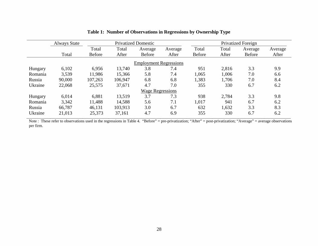
Table 1: Number of Observations in Regressions by Ownership Type

Always State Pri tic Pr gn vatized Domes ivatized Forei Average Average Average Average

Total Total

Before Total After Before After

Total Before

Total After Before After

Employment RegressionsHungary 6,102 6,956 13,740 7.4 951 2,816 3.3 9.9

nia 3,539 5.8 7.4 1,065 1,006 7.0 90 10 6.8 6.8 1,383 1,706

ne 2 4.7 7.0 6.7 W e Regressio

3.8 Roma 11,986 15,366 6.6Russia ,000 107,263 6,947 7.0 8.4Ukrai 2,068 25,575 37,671 355 330 6.2

ag nsHungary 6,014 6,881 7.3 938 2,784 3.3 9.8 Romania 3,342 11,488 14,588 7.1 1,017 941 6.7 6.2

66 46,131 10 3.0 6.7 6 1,632 e 21 4.7 6.9 355 3 6.7

13,519 3.7 5.6

Russia ,787 3,913 32 3.3 8.3Ukrain ,013 25,373 37,161 30 6.2Note : per firm

These refer to vations used regressio able 4. “B ore” = pre-pri ization; “After post-privatiz n; “Avera = average ob vations .

obser in the ns in T ef vat ” = atio ge” ser

28

Table 2: Mean Employment and Wage

Employment Wage (2004 US$)

327 9,809 Hungary (861) (8,421)

614 3,276 Romania (1,468) (14,051)

574 2,507 Russia (2,062) (4,224)

464 718 Ukraine (1,552) (3,654) Notes: Precise definitions and sources are given in Section 2. Standard deviations are shown in parentheses.

Table 3: Percentage of Firms Privatized – Majority Domestic Private and Majority Foreign

1992 1994 2004 Hungary Domestic 36.3 62.5 74.7 Foreign 6.6 11.7 16.5 Romania Domestic 0.0 10.8 86.4 Foreign 0.0 0.1 6.7 Russia Domestic 0.0 74.5 58.0 Foreign 0.0 0.9 1.2 Ukraine Domestic 0.1 13.0 74.0 Foreign 0.0 0.1 1.0

Notes: “Foreign” refers to privatized firms with more than 50% foreign-owned shares at the end of the year. “Domestic” consists of privatized firms that are not majority foreign; most of these are majority-owned by domestic private owners, but some of them also have minority foreign ownership.

29

Table 4: Estimated Employment and Wage Effects of Privatization

Hungary Romania Russia Ukraine OLS Employment δ̂ d -0.493** 0.063 1.001** 0.194** (0.064) (0.059) (0.017) (0.032) δ̂ f 0.555** 0.765** 1.708** 1.620** (0.109) (0.134) (0.099) (0.174) Pr( δ̂ f = δ̂ d ) 0.000 0.000 0.000 0.000 FE δ̂ d -0.045 0.157** 0.010 -0.062** (0.032) (0.029) (0.009) (0.017) δ̂ f 0.441** 0.376** 0.236** 0.330** (0.068) (0.091) (0.050) (0.128) Pr( δ̂ f = δ̂ d ) 0.000 0.017 0.000 0.002 FE&FT δ̂ d -0.020 -0.015 0.051** -0.004 (0.019) (0.016) (0.006) (0.012) δ̂ f 0.110** -0.071 0.137** 0.108 (0.041) (0.062) (0.039) (0.110) Pr( δ̂ f = δ̂ d ) 0.003 0.383 0.029 0.312 N 30,565 32,962 307,299 85,999 OLS Wage δ̂ d -0.023 0.018 0.194** -0.038* (0.018) (0.017) (0.011) (0.015) δ̂ f 0.482** 0.322** 0.615** 0.716** (0.030) (0.048) (0.054) (0.107) Pr( δ̂ f = δ̂ d ) 0.000 0.000 0.000 0.000 FE δ̂ d -0.045** -0.019* -0.034** -0.050** (0.014) (0.010) (0.008) (0.010) δ̂ f 0.283** 0.196** 0.315** 0.388** (0.027) (0.047) (0.045) (0.085) Pr( δ̂ f = δ̂ d ) 0.000 0.000 0.000 0.000 FE&FT δ̂ d -0.037** -0.021* -0.071** -0.025* (0.012) (0.008) (0.007) (0.011) δ̂ f 0.129** 0.093* 0.072 0.220* (0.025) (0.038) (0.041) (0.096) Pr( δ̂ f = δ̂ d ) 0.000 0.003 0.000 0.011 N 30,136 31,376 219,095 84,232

Notes: Number of firms in the employment (wage) regressions are 3,718 (3,639) Hungarian, 2,711 (2,627) Romanian, 26,402 (25,835) Russian, and 8,688 (8,437) Ukrainian firms. FE=firm fixed effects; FT=firm-specific trends. Standard errors (corrected for firm clustering) are shown in parentheses. The P values for the F test on the difference between the Foreign and Domestic coefficients are reported below the foreign standard errors. * = significant at 5-percent level. ** = significant at 1-percent level.

30

Table 5: Regressions with Zeros Imputed for Exiting Firms

Hungary Romania Russia Ukraine Employment δ̂ d -0.124** 0.075** 0.029** -0.047** (0.021) (0.015) (0.007) (0.011) δ̂ f 0.247** 0.225** 0.207** 0.214** (0.048) (0.054) (0.037) (0.062) Pr( δ̂ f = δ̂ d ) 0.000 0.007 0.000 0.000 N 30,565 32,962 307,299 85,999 Employment, exit year = 0 δ̂ d -0.063** 0.083** 0.021** -0.043** (0.020) (0.015) (0.007) (0.011) δ̂ f 0.323** 0.233** 0.232** 0.229** (0.048) (0.053) (0.037) (0.065) Pr( δ̂ f = δ̂ d ) 0.000 0.006 0.000 0.000 N 33,234 33,941 322,030 88,105 Wage δ̂ d -0.069** -0.033** -0.039** -0.050** (0.014) (0.010) (0.007) (0.009) δ̂ f 0.228** 0.155** 0.310** 0.293** (0.026) (0.035) (0.042) (0.067) Pr( δ̂ f = δ̂ d ) 0.000 0.000 0.000 0.000 N 30,136 31,376 219,095 84,232 Wage, exit year = 0 δ̂ d 0.022 0.008 -0.050** -0.042** (0.014) (0.010) (0.007) (0.009) δ̂ f 0.360** 0.198** 0.349** 0.323** (0.029) (0.035) (0.043) (0.068) Pr( δ̂ f = δ̂ d ) 0.000 0.000 0.000 0.000 N 32,823 32,355 235,387 86,423

Notes: The dependent variables are not logged, and they are divided by the firms’ means. The regressions include firm fixed effects and industry-year dummies. Standard errors (corrected for firm clustering) are shown in parentheses. Foreign = 1 if the majority of shares are foreign-owned at the beginning of year t. Domestic = 1 if private, but not majority-owned by foreigners, in the beginning of year t. The P values for the F test on the difference between the Foreign and Domestic coefficients are reported below the foreign standard errors. * = significant at 5-percent level. ** = significant at 1-percent level.

31

Appendix A: Preprivatization Characteristics of Firms Later Privatized

To provide diagnostic information about possible selection bias in the data, we estimate variants of equation (1) where the sample is restricted to state-owned firms (either never or not yet privatized, so that the single post dummy variable Privateit-1 = 0). We set wt ≡ 0, and θit ≡ (Pre-Domesticit, Pre-Foreignit). We retain the full set of industry-year interactions, Djt, so that all effects are measured within industry-year cells. Under these assumptions, employment and wage differences between firms never privatized and those privatized in the future can be estimated from the equation yit = Djtγjt + θitδ + uit. (A1) The table shows that the estimated differences vary greatly across countries, ownership types, and dependent variables. Hungarian firms domestically privatized by the end of the period tend to have much smaller employment and somewhat lower wages than the average always state-owned firm, but the pre-domestic effect on employment and wages is positive elsewhere. The foreign results are more consistent, as firms that will be foreign-owned have higher employment and wages than either pre-domestic firms or always state firms in all four countries.

Hungary Romania Russia Ukraine Employment Pre-Domestic -0.436** 0.614** 0.693** 0.205** (0.057) (0.095) (0.019) (0.039) Pre-Foreign 0.501** 1.133** 1.324** 1.327** (0.129) (0.159) (0.088) (0.168) Pr( δ̂ f = δ̂ d ) 0.000 0.000 0.000 0.000 N 14,009 16,590 198,646 47,998 Wage Pre-Domestic -0.045** 0.104** 0.123** 0.024 (0.014) (0.023) (0.012) (0.015) Pre-Foreign 0.092** 0.253** 0.251** 0.223** (0.029) (0.034) (0.037) (0.072) Pr( δ̂ f = δ̂ d ) 0.000 0.000 0.000 0.005 N 13,833 15,847 113,550 46,741 Notes: All regressions include industry-year effects. Estimates of Equation (A1). Standard errors (corrected for firm clustering) are shown in parentheses. The P values for the F test on the difference between the Foreign and Domestic coefficients are reported below the foreign standard errors. * = significant at 5-percent level. ** = significant at 1-percent level.

32

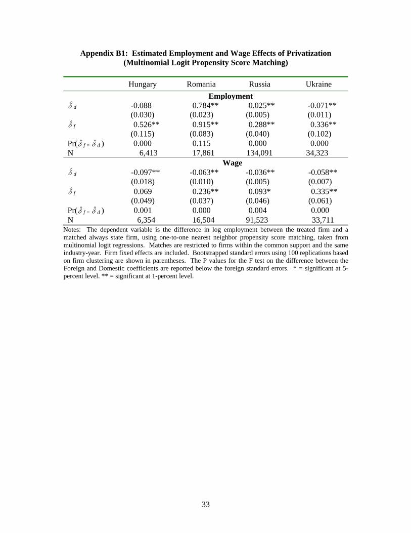
Appendix B1: Estimated Employment and Wage Effects of Privatization (Multinomial Logit Propensity Score Matching)

Hungary Romania Russia Ukraine

Employment δ̂ d -0.088 0.784** 0.025** -0.071** (0.030) (0.023) (0.005) (0.011) δ̂ f 0.526** 0.915** 0.288** 0.336** (0.115) (0.083) (0.040) (0.102) Pr( δ̂ f = δ̂ d ) 0.000 0.115 0.000 0.000 N 6,413 17,861 134,091 34,323 Wage δ̂ d -0.097** -0.063** -0.036** -0.058** (0.018) (0.010) (0.005) (0.007) δ̂ f 0.069 0.236** 0.093* 0.335** (0.049) (0.037) (0.046) (0.061) Pr( δ̂ f = δ̂ d ) 0.001 0.000 0.004 0.000 N 6,354 16,504 91,523 33,711

Notes: The dependent variable is the difference in log employment between the treated firm and a matched always state firm, using one-to-one nearest neighbor propensity score matching, taken from multinomial logit regressions. Matches are restricted to firms within the common support and the same industry-year. Firm fixed effects are included. Bootstrapped standard errors using 100 replications based on firm clustering are shown in parentheses. The P values for the F test on the difference between the Foreign and Domestic coefficients are reported below the foreign standard errors. * = significant at 5-percent level. ** = significant at 1-percent level.

33

Appendix B2: Estimated Employment and Wage Effects of Privatization (Multinomial Logit Propensity Score Matching without Trends)

Hungary Romania Russia Ukraine

Employment δ̂ d 0.080* 0.902** 0.001 -0.023* (0.034) (0.024) (0.004) (0.010) δ̂ f 0.468** 1.064** 0.276** 0.073 (0.128) (0.079) (0.051) (0.111) Pr( δ̂ f = δ̂ d ) 0.003 0.056 0.000 0.326 N 6,498 18,710 136,804 35,371 Wage δ̂ d -0.103** -0.047** -0.058** -0.057** (0.015) (0.011) (0.005) (0.008) δ̂ f 0.147** 0.169** 0.084 0.150* (0.047) (0.037) (0.046) (0.073) Pr( δ̂ f = δ̂ d ) 0.000 0.000 0.000 0.007 N 6,417 17,198 100,382 34,724

Notes: The dependent variable is the difference in log employment between the treated firm and a matched always state firm, using one-to-one nearest neighbor propensity score matching, taken from multinomial logit regressions. Matches are restricted to firms within the common support and the same industry-year. Firm fixed effects are included. Bootstrapped standard errors using 100 replications based on firm clustering are shown in parentheses. The P values for the F test on the difference between the Foreign and Domestic coefficients are reported below the foreign standard errors. * = significant at 5-percent level. ** = significant at 1-percent level.

34

Appendix B3: Estimated Employment and Wage Effects of Privatization (Multinomial Logit Propensity Score Matching

with Propensity Score Differences <=0.05)

Hungary Romania Russia Ukraine Employment δ̂ d -0.077* 0.750** 0.023** -0.071** (0.031) (0.026) (0.004) (0.011) δ̂ f 0.527** 0.877** 0.292** 0.336** (0.145) (0.086) (0.043) (0.105) Pr( δ̂ f = δ̂ d ) 0.000 0.162 0.000 0.000 N 5,789 14,565 133,308 34,224 Wage δ̂ d -0.105** -0.045** -0.042** -0.057** (0.014) (0.011) (0.005) (0.007) δ̂ f -0.029 0.284** 0.079 0.335** (0.053) (0.047) (0.046) (0.062) Pr( δ̂ f = δ̂ d ) 0.206 0.000 0.005 0.000 N 5,738 13,530 90,948 33,615 Notes: The dependent variable is the difference in log employment between the treated firm and a matched always state firm, using one-to-one nearest neighbor propensity score matching, taken from multinomial logit regressions. Matches are restricted to firms within the common support, the same industry-year, and differences in propensity scores of no more than 0.05. Firm fixed effects are included. Bootstrapped standard errors using 100 replications based on firm clustering are shown in parentheses. The P values for the F test on the difference between the Foreign and Domestic coefficients are reported below the foreign standard errors. * = significant at 5-percent level. ** = significant at 1-percent level.

35

Appendix C: Pre-Privatization Coefficients

Hungary Romania Russia Ukraine OLS Employment

-0.612** 0.173** 0.439** 0.081**δ̂ d τ-4(0.064) (0.050) (0.014) (0.030) -0.567** 0.200** 0.549** 0.121**δ̂ d τ-3(0.062) (0.053) (0.018) (0.030) -0.606** 0.148** 0.566** 0.136**δ̂ d τ-2(0.061) (0.058) (0.018) (0.030) 39.00 8.31 369.58 8.66 Domestic F test (0.000) (0.000) (0.000) (0.000) 0.524** 0.713** 1.233** 1.232**δ̂ f τ-4

(0.193) (0.138) (0.097) (0.224) 0.335 0.675** 1.311** 1.279**δ̂ fτ-3

(0.179) (0.142) (0.095) (0.208) 0.396* 0.755** 1.195** 1.274**δ̂ f τ-2

(0.159) (0.139) (0.104) (0.191) 3.32 15.20 66.02 16.35 Foreign F test

(0.019) (0.000) (0.000) (0.000) FE

0.035 0.085** -0.017** -0.041* δ̂ d τ-4(0.069) (0.032) (0.005) (0.017) 0.014 0.111** -0.032** -0.071**δ̂ d τ-3

(0.075) (0.040) (0.007) (0.021) 0.041 0.178** -0.035** -0.088**δ̂ d τ-2

(0.082) (0.050) (0.009) (0.025) 0.71 8.11 6.04 4.84 Domestic F test

(0.546) (0.000) (0.000) (0.002) -0.152 0.261** 0.024 0.032 δ̂ f τ-4(0.115) (0.067) (0.025) (0.097) -0.168 0.299** 0.034 0.060 δ̂ fτ-3(0.124) (0.082) (0.030) (0.128) -0.051 0.408** -0.050 0.039 δ̂ f τ-2(0.139) (0.091) (0.044) (0.148)

Foreign F test 0.86 8.12 3.36 0.19 (0.461) (0.000) (0.018) (0.902) FE&FT

0.048 -0.018 0.007 -0.020 δ̂ d τ-4(0.044) (0.020) (0.005) (0.014) 0.006 -0.023 0.014 -0.040* δ̂ d τ-3

(0.052) (0.028) (0.009) (0.019) -0.002 -0.019 0.019 -0.058* δ̂ d τ-2(0.061) (0.035) (0.011) (0.024) 2.38 0.62 0.89 2.36 Domestic F test

(0.068) (0.603) (0.445) (0.070) -0.129 -0.035 0.006 -0.066 δ̂ f τ-4(0.069) (0.048) (0.035) (0.068) -0.195** -0.105 0.032 -0.109 δ̂ fτ-3(0.077) (0.072) (0.051) (0.124) -0.200* -0.132 0.015 -0.102 δ̂ f τ-2(0.096) (0.098) (0.067) (0.152) 2.34 1.59 1.23 0.46 Foreign F test

(0.072) (0.190) (0.295) (0.714)

36

Appendix C (continued)

Hungary Romania Russia Ukraine Matching & FE Employment

0.263** 0.041 0.004 0.027 δ̂ d τ-4(0.065) (0.035) (0.005) (0.023) 0.227** 0.045 0.000 0.002 δ̂ d τ-3

(0.062) (0.031) (0.006) (0.021) 0.174** 0.124** 0.015* -0.016 δ̂ d τ-2

(0.067) (0.035) (0.006) (0.019) 25.91 12.82 7.29 6.17 Domestic F test (0.000) 0.005 (0.063) (0.104) -0.184 0.227 0.004 0.163 δ̂ f τ-4(0.204) (0.118) (0.074) (0.169) -0.140 0.152 -0.031 0.179 δ̂ fτ-3(0.200) (0.119) (0.067) (0.165) -0.041 0.212* -0.042 0.265* δ̂ f τ-2(0.177) (0.101) (0.063) (0.135) 1.34 5.52 0.63 3.85 Foreign F test

(0.720) (0.138) (0.890) (0.278)

37

Appendix C (continued)

Hungary Romania Russia Ukraine OLS Wage

-0.051** 0.038** 0.029** -0.011 δ̂ d τ-4(0.016) (0.013) (0.007) (0.013) -0.056** 0.052** 0.100** -0.001 δ̂ d τ-3(0.016) (0.014) (0.030) (0.014) -0.037* 0.061** 0.171** 0.011 δ̂ d τ-2(0.018) (0.015) (0.014) (0.014) 4.63 5.89 56.32 1.85 Domestic F test

(0.003) (0.001) (0.000) (0.136) 0.115** 0.191** 0.102 0.254**δ̂ f τ-4

(0.045) (0.034) (0.061) (0.098) 0.089 0.218** 0.401** 0.351**δ̂ fτ-3

(0.049) (0.037) (0.114) (0.103) 0.093 0.239** 0.309** 0.288**δ̂ f τ-2

(0.051) (0.034) (0.063) (0.093) 2.57 16.79 10.25 4.52 Foreign F test

(0.053) (0.000) (0.000) (0.004) FE

0.037 0.012 0.053** -0.022 δ̂ d τ-4(0.024) (0.013) (0.013) (0.012) 0.032 0.014 0.058** -0.027* δ̂ d τ-3

(0.026) (0.015) (0.021) (0.014) 0.050 0.024 0.079** -0.027 δ̂ d τ-2

(0.029) (0.018) (0.018) (0.015) 1.24 0.76 9.33 1.46 Domestic F test

(0.294) (0.517) (0.000) (0.225) 0.120** 0.025 0.044 0.078 δ̂ f τ-4

(0.045) (0.030) (0.105) (0.069) 0.098 0.065 0.072 0.146 δ̂ fτ-3

(0.054) (0.036) (0.117) (0.089) 0.127* 0.084** 0.090 0.036 δ̂ f τ-2

(0.056) (0.031) (0.087) (0.080) Foreign F test 2.86 3.06 0.43 1.43 (0.036) (0.027) (0.730) (0.233) FE&FT

-0.047 0.001 -0.012 0.009 δ̂ d τ-4(0.028) (0.012) (0.015) (0.012) -0.031 0.005 -0.053* 0.015 δ̂ d τ-3(0.032) (0.016) (0.022) (0.016) -0.007 0.008 -0.044* 0.027 δ̂ d τ-2(0.038) (0.020) (0.021) (0.019) 2.42 0.11 2.21 0.84 Domestic F test

(0.064) (0.957) (0.084) (0.470) 0.101* 0.007 -0.024 0.104 δ̂ f τ-4

(0.045) (0.026) (0.088) (0.053) 0.086 0.043 -0.034 0.201**δ̂ fτ-3

(0.059) (0.040) (0.109) (0.077) 0.112 0.053 -0.052 0.153* δ̂ f τ-2

(0.067) (0.047) (0.091) (0.071) 1.92 0.71 0.12 2.35 Foreign F test

(0.124) (0.546) (0.951) (0.071)

38

Appendix C (continued)

Hungary Romania Russia Ukraine Matching & FE Wage

-0.118** -0.004 0.031 -0.029 δ̂ d τ-4(0.033) (0.018) (0.019) (0.016) -0.109** -0.015 0.043 -0.053**δ̂ d τ-3(0.031) (0.016) (0.030) (0.016) -0.053 -0.037 0.050** -0.052**δ̂ d τ-2(0.034) (0.014) (0.018) (0.014) 28.93 7.23 7.83 16.43 Domestic F test (0.002) (0.065) (0.050) (0.001) 0.116 -0.033 0.042 0.061 δ̂ f τ-4

(0.073) (0.053) (0.101) (0.101) 0.021 -0.028 0.060 0.165 δ̂ fτ-3

(0.087) (0.060) (0.096) (0.117) 0.059 0.011 -0.057 -0.022 δ̂ f τ-2

(0.086) (0.052) (0.097) (0.102) 2.85 0.92 1.16 3.00 Foreign F test

(0.415) (0.821) (0.763) (0.391)

39

Appendix D: Estimated Effects of Privatization on the Probability of Exit

Hungary Romania Russia Ukraine δ̂ d -0.039** -0.015** 0.001 -0.006** (0.003) (0.001) (0.001) (0.001) δ̂ f -0.043** -0.009** -0.016** -0.008** (0.002) (0.001) (0.002) (0.001) Pr( δ̂ f = δ̂ d ) 0.000 0.263 0.000 0.029 R2 0.086 0.132 0.125 0.127 Mean Exit 0.081 0.029 0.070 0.027 N 33,252 33,941 234,322 81,028

Notes: Probit marginal effect estimates. Industry and year dummies are included in the regressions. Standard errors (corrected for firm clustering) are shown in parentheses. The P values for the F test on the difference between the Foreign and Domestic coefficients are reported below the foreign standard errors. ** = significant at 1-percent level.

40

Appendix E: Dynamics of Privatization Effects on Employment and Wage

Hungary Romania Russia Ukraine FE Employment

-0.030 -0.310** 0.016 0.094**δ̂ d τ-5-(0.099) (0.069) (0.012) (0.033) 0.006 -0.225** -0.002 0.052* δ̂ d τ-4

(0.048) (0.045) (0.010) (0.021) -0.015 -0.199** -0.016 0.023 δ̂ d τ-3(0.042) (0.035) (0.008) (0.016) 0.012 -0.131** -0.019** 0.006 δ̂ d τ-2

(0.032) (0.024) (0.006) (0.011) -0.029 -0.074** -0.014** 0.002 δ̂ d τ-1(0.020) (0.013) (0.004) (0.006) -0.007 0.065** 0.019** -0.003 δ̂ d τ1(0.016) (0.014) (0.004) (0.007) 0.006 0.146** 0.026** -0.034**δ̂ d τ2

(0.028) (0.025) (0.007) (0.013) -0.029 0.247** 0.031** -0.079**δ̂ d τ3(0.038) (0.036) (0.009) (0.018) -0.045 0.354** 0.010 -0.107**δ̂ d τ4(0.048) (0.048) (0.011) (0.024) -0.089 0.666** -0.024 -0.099**δ̂ d τ5+(0.068) (0.069) (0.015) (0.032) 0.101 -0.658** -0.069 -0.163 δ̂ f τ-5-

(0.148) (0.108) (0.051) (0.158) -0.051 -0.397** -0.045 -0.131 δ̂ f τ-4(0.132) (0.067) (0.042) (0.133) -0.066 -0.359** -0.035 -0.103 δ̂ f τ-3(0.111) (0.058) (0.040) (0.073) 0.051 -0.250** -0.118** -0.123**δ̂ f τ-2

(0.077) (0.042) (0.037) (0.043) 0.229** -0.136** -0.082** -0.010 δ̂ f τ-1

(0.049) (0.027) (0.020) (0.056) 0.171** 0.111** 0.053 0.091 δ̂ f τ1

(0.032) (0.031) (0.029) (0.070) 0.290** 0.212** 0.099* 0.097 δ̂ f τ2

(0.050) (0.067) (0.037) (0.097) 0.400** 0.327** 0.190** 0.155 δ̂ f τ3

(0.056) (0.081) (0.039) (0.104) 0.434** 0.418** 0.207** 0.032 δ̂ f τ4

(0.065) (0.104) (0.040) (0.154) 0.674** 0.672** 0.183** 0.021 δ̂ f τ5+

(0.091) (0.136) (0.065) (0.239) N 28,832 31,979 306,139 80,260

41

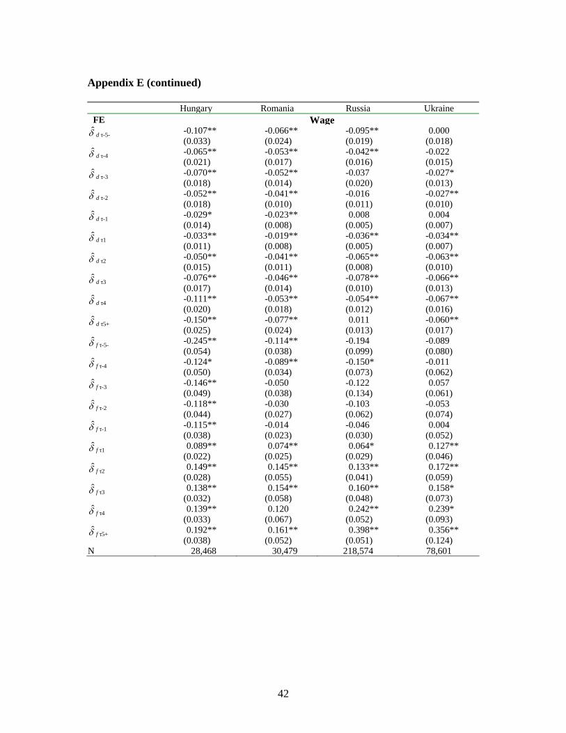
Appendix E (continued)

Hungary Romania Russia Ukraine FE Wage

-0.107** -0.066** -0.095** 0.000 δ̂ d τ-5-(0.033) (0.024) (0.019) (0.018) -0.065** -0.053** -0.042** -0.022 δ̂ d τ-4(0.021) (0.017) (0.016) (0.015) -0.070** -0.052** -0.037 -0.027* δ̂ d τ-3(0.018) (0.014) (0.020) (0.013) -0.052** -0.041** -0.016 -0.027**δ̂ d τ-2(0.018) (0.010) (0.011) (0.010) -0.029* -0.023** 0.008 0.004 δ̂ d τ-1(0.014) (0.008) (0.005) (0.007) -0.033** -0.019** -0.036** -0.034**δ̂ d τ1(0.011) (0.008) (0.005) (0.007) -0.050** -0.041** -0.065** -0.063**δ̂ d τ2(0.015) (0.011) (0.008) (0.010) -0.076** -0.046** -0.078** -0.066**δ̂ d τ3(0.017) (0.014) (0.010) (0.013) -0.111** -0.053** -0.054** -0.067**δ̂ d τ4(0.020) (0.018) (0.012) (0.016) -0.150** -0.077** 0.011 -0.060**δ̂ d τ5+(0.025) (0.024) (0.013) (0.017) -0.245** -0.114** -0.194 -0.089 δ̂ f τ-5-(0.054) (0.038) (0.099) (0.080) -0.124* -0.089** -0.150* -0.011 δ̂ f τ-4(0.050) (0.034) (0.073) (0.062) -0.146** -0.050 -0.122 0.057 δ̂ f τ-3(0.049) (0.038) (0.134) (0.061) -0.118** -0.030 -0.103 -0.053 δ̂ f τ-2(0.044) (0.027) (0.062) (0.074) -0.115** -0.014 -0.046 0.004 δ̂ f τ-1(0.038) (0.023) (0.030) (0.052) 0.089** 0.074** 0.064* 0.127**δ̂ f τ1

(0.022) (0.025) (0.029) (0.046) 0.149** 0.145** 0.133** 0.172**δ̂ f τ2

(0.028) (0.055) (0.041) (0.059) 0.138** 0.154** 0.160** 0.158* δ̂ f τ3

(0.032) (0.058) (0.048) (0.073) 0.139** 0.120 0.242** 0.239* δ̂ f τ4

(0.033) (0.067) (0.052) (0.093) 0.192** 0.161** 0.398** 0.356**δ̂ f τ5+

(0.038) (0.052) (0.051) (0.124) N 28,468 30,479 218,574 78,601

42

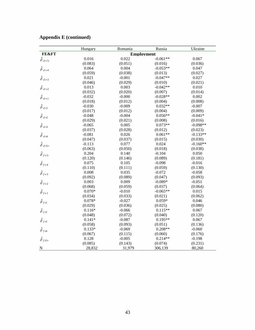
Appendix E (continued)

Hungary Romania Russia Ukraine FE&FT Employment

0.016 0.022 -0.061** 0.067 δ̂ d τ-5-(0.083) (0.051) (0.016) (0.036) 0.064 0.004 -0.053** 0.047 δ̂ d τ-4

(0.059) (0.038) (0.013) (0.027) 0.021 -0.001 -0.047** 0.027 δ̂ d τ-3

(0.046) (0.029) (0.010) (0.021) 0.013 0.003 -0.042** 0.010 δ̂ d τ-2

(0.032) (0.020) (0.007) (0.014) -0.032 -0.000 -0.028** 0.002 δ̂ d τ-1(0.018) (0.012) (0.004) (0.008) -0.030 -0.009 0.032** -0.007 δ̂ d τ1(0.017) (0.012) (0.004) (0.009) -0.048 -0.004 0.056** -0.041* δ̂ d τ2(0.029) (0.021) (0.008) (0.016) -0.065 0.005 0.073** -0.098**δ̂ d τ3(0.037) (0.028) (0.012) (0.023) -0.081 0.026 0.061** -0.133**δ̂ d τ4(0.047) (0.037) (0.015) (0.030) -0.113 0.077 0.024 -0.160**δ̂ d τ5+(0.063) (0.050) (0.018) (0.038) 0.204 0.140 -0.104 0.050 δ̂ f τ-5-

(0.120) (0.146) (0.089) (0.181) 0.075 0.105 -0.098 -0.016 δ̂ f τ-4

(0.110) (0.111) (0.059) (0.130) 0.008 0.035 -0.072 -0.058 δ̂ f τ-3

(0.092) (0.089) (0.047) (0.093) 0.003 0.009 -0.089* -0.051 δ̂ f τ-2

(0.068) (0.059) (0.037) (0.064) 0.070* -0.010 -0.065** 0.015 δ̂ f τ-1

(0.034) (0.033) (0.021) (0.062) 0.078* -0.027 0.059* 0.046 δ̂ f τ1

(0.029) (0.036) (0.025) (0.080) 0.116* -0.066 0.115** 0.067 δ̂ f τ2

(0.048) (0.072) (0.040) (0.120) 0.141* -0.087 0.195** 0.067 δ̂ f τ3

(0.058) (0.093) (0.051) (0.136) 0.133* -0.069 0.208** -0.060 δ̂ f τ4

(0.067) (0.115) (0.060) (0.176) 0.128 -0.005 0.214** -0.198 δ̂ f τ5+

(0.085) (0.143) (0.074) (0.231) N 28,832 31,979 306,139 80,260

43

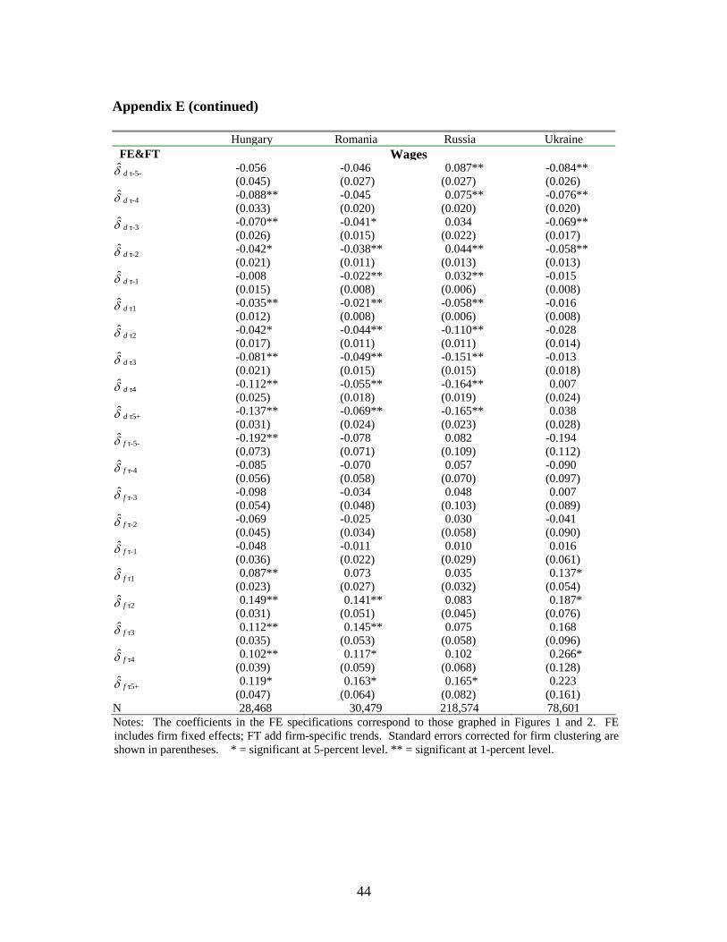
Appendix E (continued)

Hungary Romania Russia Ukraine FE&FT Wages

-0.056 -0.046 0.087** -0.084**δ̂ d τ-5-(0.045) (0.027) (0.027) (0.026) -0.088** -0.045 0.075** -0.076**δ̂ d τ-4(0.033) (0.020) (0.020) (0.020) -0.070** -0.041* 0.034 -0.069**δ̂ d τ-3(0.026) (0.015) (0.022) (0.017) -0.042* -0.038** 0.044** -0.058**δ̂ d τ-2(0.021) (0.011) (0.013) (0.013) -0.008 -0.022** 0.032** -0.015 δ̂ d τ-1(0.015) (0.008) (0.006) (0.008) -0.035** -0.021** -0.058** -0.016 δ̂ d τ1(0.012) (0.008) (0.006) (0.008) -0.042* -0.044** -0.110** -0.028 δ̂ d τ2(0.017) (0.011) (0.011) (0.014) -0.081** -0.049** -0.151** -0.013 δ̂ d τ3(0.021) (0.015) (0.015) (0.018) -0.112** -0.055** -0.164** 0.007 δ̂ d τ4(0.025) (0.018) (0.019) (0.024) -0.137** -0.069** -0.165** 0.038 δ̂ d τ5+(0.031) (0.024) (0.023) (0.028) -0.192** -0.078 0.082 -0.194 δ̂ f τ-5-(0.073) (0.071) (0.109) (0.112) -0.085 -0.070 0.057 -0.090 δ̂ f τ-4(0.056) (0.058) (0.070) (0.097) -0.098 -0.034 0.048 0.007 δ̂ f τ-3(0.054) (0.048) (0.103) (0.089) -0.069 -0.025 0.030 -0.041 δ̂ f τ-2(0.045) (0.034) (0.058) (0.090) -0.048 -0.011 0.010 0.016 δ̂ f τ-1(0.036) (0.022) (0.029) (0.061) 0.087** 0.073 0.035 0.137* δ̂ f τ1

(0.023) (0.027) (0.032) (0.054) 0.149** 0.141** 0.083 0.187* δ̂ f τ2

(0.031) (0.051) (0.045) (0.076) 0.112** 0.145** 0.075 0.168 δ̂ f τ3

(0.035) (0.053) (0.058) (0.096) 0.102** 0.117* 0.102 0.266* δ̂ f τ4

(0.039) (0.059) (0.068) (0.128) 0.119* 0.163* 0.165* 0.223 δ̂ f τ5+

(0.047) (0.064) (0.082) (0.161) N 28,468 30,479 218,574 78,601 Notes: The coefficients in the FE specifications correspond to those graphed in Figures 1 and 2. FE includes firm fixed effects; FT add firm-specific trends. Standard errors corrected for firm clustering are shown in parentheses. * = significant at 5-percent level. ** = significant at 1-percent level.

44

Appendix F: Decomposition of Privatization Effect on Employment

Hungary Romania Russia Ukraine

FE Employment δ̂ d -0.071** 0.108** 0.015 -0.050** (0.029) (0.026) (0.008) (0.015) δ̂ f 0.361** 0.320** 0.220** 0.311** (0.063) (0.084) (0.043) (0.102) Pr( δ̂ f = δ̂ d ) 0.000 0.012 0.000 0.000 FE&FT δ̂ d -0.020 -0.010 0.044** 0.001 (0.018) (0.015) (0.005) (0.010) δ̂ f 0.073 -0.048 0.106** 0.090 (0.039) (0.052) (0.030) (0.080) Pr( δ̂ f = δ̂ d ) 0.026 0.487 0.037 0.262 FE Output δ̂ d 0.019 0.335** -0.051** -0.019 (0.034) (0.038) (0.017) (0.026) δ̂ f 0.912** 0.794** 0.652** 0.852** (0.072) (0.113) (0.087) (0.227) Pr( δ̂ f = δ̂ d ) 0.000 0.000 0.000 0.000 FE&FT δ̂ d 0.063** 0.085** -0.030** -0.015 (0.022) (0.024) (0.011) (0.019) δ̂ f 0.286** 0.144 0.190** 0.337 (0.050) (0.080) (0.062) (0.221) Pr( δ̂ f = δ̂ d ) 0.000 0.477 0.000 0.112 FE Labor Productivity δ̂ d 0.089** 0.227** -0.067** 0.031 (0.020) (0.022) (0.013) (0.021) δ̂ f 0.551** 0.475** 0.432** 0.541** (0.041) (0.073) (0.072) (0.181) Pr( δ̂ f = δ̂ d ) 0.000 0.001 0.000 0.005 FE&FT δ̂ d 0.083** 0.096** -0.074** -0.016 (0.019) (0.017) (0.010) (0.017) δ̂ f 0.213** 0.191** 0.084 0.246 (0.035) (0.064) (0.054) (0.196) Pr( δ̂ f = δ̂ d ) 0.000 0.147 0.003 0.180 N 30,098 32,076 294,767 81,589

Notes: The FE&FT coefficient estimates correspond to those reported in Figures 1-4, while the standard errors and FE estimates supplement those results. Other notes are same as in Table 4. * = significant at 5-percent level. ** = significant at 1-percent level.

45

Appendix G: Decomposition of Privatization Effect on Wage

Hungary Romania Russia Ukraine FE Wage δ̂ d -0.044** -0.027** -0.035** -0.047** (0.013) (0.009) (0.007) (0.010) δ̂ f 0.295** 0.177** 0.330** 0.391** (0.027) (0.042) (0.043) (0.086) Pr( δ̂ f = δ̂ d ) 0.000 0.000 0.000 0.000 FE&FT δ̂ d -0.038** -0.017* -0.070** -0.031** (0.012) (0.008) (0.007) (0.010) δ̂ f 0.135** 0.078* 0.080* 0.232* (0.024) (0.035) (0.040) (0.095) Pr( δ̂ f = δ̂ d ) 0.000 0.008 0.000 0.006 FE Unit Labor Cost δ̂ d -0.131** -0.254** 0.026** -0.079** (0.018) (0.021) (0.008) (0.017) δ̂ f -0.260** -0.311** -0.083 -0.146 (0.036) (0.057) (0.052) (0.145) Pr( δ̂ f = δ̂ d ) 0.000 0.324 0.034 0.646 FE&FT δ̂ d -0.116** -0.111** -0.012 -0.018 (0.016) (0.017) (0.007) (0.014) δ̂ f -0.081** -0.111* 0.076 -0.033 (0.032) (0.054) (0.045) (0.152) Pr( δ̂ f = δ̂ d ) 0.319 0.993 0.052 0.923 FE Labor Productivity δ̂ d 0.088** 0.227** -0.061** 0.032 (0.020) (0.022) (0.011) (0.021) δ̂ f 0.555** 0.488** 0.413** 0.537** (0.042) (0.074) (0.069) (0.181) Pr( δ̂ f = δ̂ d ) 0.000 0.000 0.000 0.005 FE&FT δ̂ d 0.078** 0.094** -0.058** -0.012 (0.018) (0.018) (0.009) (0.017) δ̂ f 0.216** 0.189** 0.004 0.265 (0.036) (0.066) (0.052) (0.196) Pr( δ̂ f = δ̂ d ) 0.000 0.158 0.237 0.157 N 29,810 30,774 212,042 80,500

Notes: The FE&FT coefficient estimates correspond to those reported in Figures 1-4, while the standard errors and FE estimates supplement those results. Other notes are same as in Table 4. * = significant at 5-percent level. ** = significant at 1-percent level.

46