Empirical Industrial Organization - econ.msu.ru · { Market size de nition (merger analysis); ... In this case Pr(ichoose j) = Z A j(X;p) ... REDBUS would also have high BLUEBUS

Empirical Industrial Organization

Notes for Summer SchoolMoscow State University, Faculty of Economics

Andrey Simonov∗

June 2013

Attributions: This notes gained a lot from various courses in Tilburg University and Uni-versity of Chicago, in particular courses by Bart Bronnenberg, Jaap Abbring, Tobias Klein,Derek Niel, Ali Hortacsu, Jean-Piere Dube, Guenter Hitsch and Pradeep Chintagunta. Sec-tion on production function function heavily relies on excellent review by Ackerberg et al.(2007). Of course, all errors and typos are of my own1.

c©Andrey D. Simonov, 2013∗University of Chicago, Booth School of Business1Please send any comments/reports on typos to [email protected]

1

CONTENTS CONTENTS

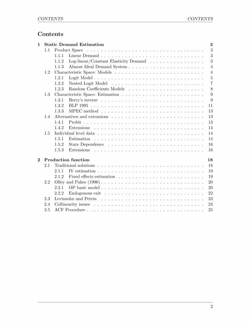
Contents

1 Static Demand Estimation 31.1 Product Space . . . . . . . . . . . . . . . . . . . . . . . . . . . . . . . . . . 3

1.1.1 Linear Demand . . . . . . . . . . . . . . . . . . . . . . . . . . . . . . 31.1.2 Log-linear/Constant Elasticity Demand . . . . . . . . . . . . . . . . 31.1.3 Almost Ideal Demand System . . . . . . . . . . . . . . . . . . . . . . 4

1.2 Characteristic Space: Models . . . . . . . . . . . . . . . . . . . . . . . . . . 41.2.1 Logit Model . . . . . . . . . . . . . . . . . . . . . . . . . . . . . . . . 51.2.2 Nested Logit Model . . . . . . . . . . . . . . . . . . . . . . . . . . . 71.2.3 Random Coefficients Models . . . . . . . . . . . . . . . . . . . . . . 8

1.3 Characteristic Space: Estimation . . . . . . . . . . . . . . . . . . . . . . . . 91.3.1 Berry’s inverse . . . . . . . . . . . . . . . . . . . . . . . . . . . . . . 91.3.2 BLP 1995 . . . . . . . . . . . . . . . . . . . . . . . . . . . . . . . . . 111.3.3 MPEC method . . . . . . . . . . . . . . . . . . . . . . . . . . . . . . 13

1.4 Alternatives and extensions . . . . . . . . . . . . . . . . . . . . . . . . . . . 131.4.1 Probit . . . . . . . . . . . . . . . . . . . . . . . . . . . . . . . . . . . 131.4.2 Extensions . . . . . . . . . . . . . . . . . . . . . . . . . . . . . . . . 14

1.5 Individual level data . . . . . . . . . . . . . . . . . . . . . . . . . . . . . . . 141.5.1 Estimation . . . . . . . . . . . . . . . . . . . . . . . . . . . . . . . . 141.5.2 State Dependence . . . . . . . . . . . . . . . . . . . . . . . . . . . . 161.5.3 Extensions . . . . . . . . . . . . . . . . . . . . . . . . . . . . . . . . 16

2 Production function 182.1 Traditional solutions . . . . . . . . . . . . . . . . . . . . . . . . . . . . . . . 18

2.1.1 IV estimation . . . . . . . . . . . . . . . . . . . . . . . . . . . . . . . 192.1.2 Fixed effects estimation . . . . . . . . . . . . . . . . . . . . . . . . . 19

2.2 Olley and Pakes (1996) . . . . . . . . . . . . . . . . . . . . . . . . . . . . . . 202.2.1 OP basic model . . . . . . . . . . . . . . . . . . . . . . . . . . . . . . 202.2.2 Endogenous exit . . . . . . . . . . . . . . . . . . . . . . . . . . . . . 22

2.3 Levinsohn and Petrin . . . . . . . . . . . . . . . . . . . . . . . . . . . . . . 232.4 Collinearity issues . . . . . . . . . . . . . . . . . . . . . . . . . . . . . . . . 242.5 ACF Procedure . . . . . . . . . . . . . . . . . . . . . . . . . . . . . . . . . . 25

2

1 STATIC DEMAND ESTIMATION

1 Static Demand Estimation

• Why do we care about demand system estimation? One of the key ingredients in anumber of Industrial Organization (IO) questions. I.e.:

– Entry/exit decisions;

– Market size definition (merger analysis);

– Production decisions.

• Lets focus on the differentiated product markets.

• Consider the market with J heterogeneous goods.

• There are two ways to proceed with estimation: treat each product as a good itself,or treat a product as a bundle of characteristics.

1.1 Product Space

1.1.1 Linear Demand

• Think about a market with j goods: j = 1, · · · , J . Proposed demand equation:

qi = ai +∑j

bijpij + εij

where qi is demand for good i, pij are price coefficients, bij are marginal effects, aiare product-specific intercepts and εij are the random shocks.

• Allow to compute own and cross price elasticities.

• The most obvious problem: we can get negative value for qi

1.1.2 Log-linear/Constant Elasticity Demand

• Solution: use log-linear/constant elasticity demand:

logqi = αi + ηilogm+

k∑j=1

εijlogpj + εi

where m is income and ηi is income elasticity

• Looks like Marshallian demand curve.

• Well, another problem: adding up constraint does not hold unless ηi = 1 ∀i:∑k

i=1wiηi =1 where wi are the expenditure shares.

3

1.2 Characteristic Space: Models 1 STATIC DEMAND ESTIMATION

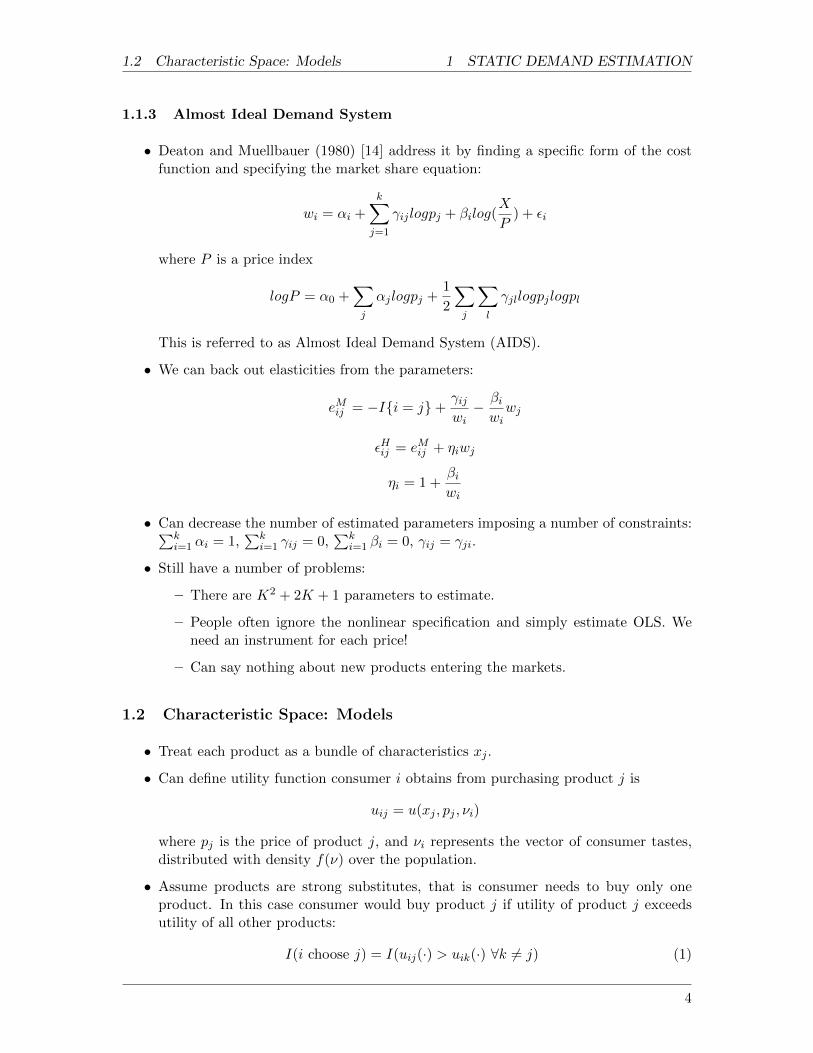
1.1.3 Almost Ideal Demand System

• Deaton and Muellbauer (1980) [14] address it by finding a specific form of the costfunction and specifying the market share equation:

wi = αi +k∑j=1

γijlogpj + βilog(X

P) + εi

where P is a price index

logP = α0 +∑j

αjlogpj +1

2

∑j

∑l

γjllogpjlogpl

This is referred to as Almost Ideal Demand System (AIDS).

• We can back out elasticities from the parameters:

eMij = −I{i = j}+γijwi− βiwiwj

εHij = eMij + ηiwj

ηi = 1 +βiwi

• Can decrease the number of estimated parameters imposing a number of constraints:∑ki=1 αi = 1,

∑ki=1 γij = 0,

∑ki=1 βi = 0, γij = γji.

• Still have a number of problems:

– There are K2 + 2K + 1 parameters to estimate.

– People often ignore the nonlinear specification and simply estimate OLS. Weneed an instrument for each price!

– Can say nothing about new products entering the markets.

1.2 Characteristic Space: Models

• Treat each product as a bundle of characteristics xj .

• Can define utility function consumer i obtains from purchasing product j is

uij = u(xj , pj , νi)

where pj is the price of product j, and νi represents the vector of consumer tastes,distributed with density f(ν) over the population.

• Assume products are strong substitutes, that is consumer needs to buy only oneproduct. In this case consumer would buy product j if utility of product j exceedsutility of all other products:

I(i choose j) = I(uij(·) > uik(·) ∀k 6= j) (1)

4


• We can define the region of f(ν) where consumers prefer product j as

Aj(X, p) = {νi ∈ RL|(uij(·) > uik(·) ∀k 6= j}

• Now we can define the market share of the good j as

sj =

∫Aj(X,p)

f(ν)dν (2)

Knowing the market share and the market size, we can easily back out the demandby

qj = Msj

• How do we solve this integral? There are two way to proceed:

– Assume a particular distribution which will make the solution analytic (i.e. logitor nested logit models)

– Use simulations or quadratures to approximate the integral.

• Similarly, as econometricians we can use distribution f(ν) to define the probabilityof consumer j choose i:

Pr(i choose j) = Pr(uij(·) > uik(·) ∀k 6= j) (3)

In this case

Pr(i choose j) =

∫Aj(X,p)

f(ν)dν

• In what follows we stick to the interpretation (2) as we discuss aggregate demand.Interpretation (3) would be useful later in the discussion of individual choice models.

1.2.1 Logit Model

• Assume additively separable utility functions:

uij = Xjβ + αpj + εij

where εij denotes consumer idiosyncratic taste for product j (which before was in-cluded into νi) (was is the dimension of εi now?)

• Assume a particular functional form for εij :

εij ∼ iid T1EV (ε)

which is Type 1 Extreme Value distribution2 with location parameter 0 and scaleparameter 1:

F (εij) = exp(−exp(−εij))2Also known as Gumbel distribution

5


• Using the properties of T1EV distribution (difference of two independent T1EV isdistributed logistically) we can write the market shares as

sj(X, p) =

∫· · ·∫Aj

f(dεi1, · · · , dεiJ) =eXjβ+αpj∑k e

Xkβ+αpk=

eδj∑k e

δk(4)

where δj is the mean utility of product j.

• We do not observe the actual utility, which requires us to make some normalizations:on the location and on the scale:

– Scale is implicitly normalized as logit error term has a fixed variance;

– Location is usually normalized by δ0 = 0, which reflects the outside option.

• Examine price derivatives and elasticities in order to characterize demand function:

Own-price marginal effect:∂qj∂pj

=∂sj∂pj

M = M

[α

eδj∑k e

δk− α(

eδj∑k e

δk)2

]= Mαsj(1−sj)

Cross-price marginal effect:∂qj∂pk

=∂sj∂pk

M = M

[−α eδjeδk

(∑

k eδk)2

]= −Mαsjsk

(Check that own and cross-price elasticities exhibit similar problems)

• Own-price derivatives vary only with the market size of good j. This is restrictive astwo products with the same market size (say BMW and Kia) should have the sameown-price elasticity (completely unintuitive in the example of BMW and Kia).

• Things are even worth in cross-price derivatives: if sBMW = sKia cross-price marginaleffect of price of Mercedes on both BMW and Kia should be the same. Obviouslymakes no sense.

• In a way market shares are ”sufficient statistics” for substitution patterns. This isoften said to be the result of the logit model; however, it rather comes from iid tastesof consumers over products:

uij = δj + εij ⇒ sj = f(δj , δ1, · · · , δJ)

sj = sk ⇒ δj = δk

• Logit models have another problem: Independence of Irrelevant Alternatives (IIA)property. It says that

sjsk

does not depend on other products.

• Classical example is when consumer needs to choose 1) between red bus and a car;2) between red bus, blue bus and a car. If sRED BUS

sCAR= 1/2 in the first model (33.3%

of consumers choose a bus), then sRED BUSsCAR

= 1/2 in the second model (but now 50%of consumers choose a bus: 25% a red bus and 25% a blue one). Once again makesno sense.

• These problems can be solved by allowing for correlation in consumer tastes, i.e.people with high εRED BUS would also have high εBLUE BUS . However, if try toestimate all elements in the variance-covariance matrix Σεi we need to estimate (J2+J)/2 elements, which is the same problem as we had in case of product space demandestimation.

6


• We can try to put some restrictions on Σεi such that the space of parameters is nottoo big.

1.2.2 Nested Logit Model

• We can use some prior knowledge about the structure of the market to divide productsinto G nests.

• Assume that nests are exclusive (product can be only in one nest).

• Redefine consumer utility as

uij = Xjβ + αpj + ζigj + (1− σ)εij = δj + νij

where

– δj = Xjβ + αpj

– νij = ζigj + (1− σ)εij

– ζjgj is a specific taste of group gj and is iid over groups.

• What is the structure of Σν?

E(νijνik) =

{σ2ζ if (j, k) ∈ g0 otherwise

• Market share is defined as in (4):

sj =

∫· · ·∫Aj

f(dζi, dεi) (5)

• Cardell (1996) [10] shows that ∀σ there exists a unique distribution of ζi such that ifεi ∼ iid EV then νij ∼ iid EV

• Nested Logit model makes this particular assumptions, which makes an integral in(5) analytical:

sj(X, p) = sj|gsg =exp(

δj1−σ )∑

k∈gj exp(δk1−σ )

(∑

k∈gj exp(δk1−σ )

)1−σ∑

g

(∑k∈gj exp(

δk1−σ )

)1−σ (6)

where sj|g stands for the market share of good j in the nest g, and sg stands for themarket share of nest g.

• Price elasticities in this case would be stronger within group than between groups(derivation is the same as for logit).

• What happens as we change σ?

– as σ → 1, substitution would be only within group;

7


– as σ → 0, we get back to logit model.

• Extensions to this include multiple level of nests (Cardell 1997 [10]), overlappingnests (Bresnahan, Stern, Trajtenberg 1997 [7]), ordered nests.

• Nested models are quite powerful. However, often criticized for setting the groupsa-priori.

1.2.3 Random Coefficients Models

• Redefine consumer utility as

uij = Xjβi − αipj + εij

Notice that now we allow both β and α to vary across consumers: intuitively wewould expect that now price elasticities should be very flexible.

• However, we need to impose some structure of βi and αi, otherwise we have (M+1)Nparameters to estimate with N observations (M is the number of characteristics).

• One way to proceed is to assume a particular distribution for βi and αi, i.e.:

– βi consist of M independent marginals, where

βim ∼ N(βm, σ2m)

– αi can be interpreted as consumer distaste for price:

lnαi ∼ N(α, σ2α)

(why do we use log-normal instead of normal in this case?)

• As before, we assume that εij ∼ iid T1EV .

• Obviously, it is a generalized version of the logit model. It also appears to be ageneralized version of the nested logit model.

• Defineβim = βm + σmβim βim ∼ N(0, 1)

αi = exp(α+ σααi) αi ∼ N(0, 1)

Now we can rewrite uij as

uij = Xjβ − αpj +

[∑m

σmxjmβim − σαpjαi + εij

]= δj + νij

• Notice that νij would be correlated across products as it contains xj and pj . Thatis, cross-price elasticities with products that have more similar characteristics wouldbe higher.

• It seems like the result we want. What are the caveats?

8

1.3 Characteristic Space: Estimation 1 STATIC DEMAND ESTIMATION

• Well, one thing is that once again we make very specific assumptions on parameters.This can be slightly improved by using empirical distribution of demographics.

• Another problem is more severe. Rewrite the market share equation:

sj =

∫· · ·∫Aj

f(dβi, αi, dεi) (7)

Unfortunately there is no analytical solution for (7). One way to go is to use quadra-tures, but these becomes infeasible as the number of integrals gets > 5 (what numberof integrals would you expect say for cola market? automobile market?)

• This is not a problem for bayesian econometrics (discussed today at the Data Analysissection).

• If we want to stay in the frequentists domain we need to simulate this integral. Foran arbitrary function f(·) and arbitrary distribution with pdf g(·):

Y =

∫f(z)g(z)dz ≈ 1

NS

∑NS

f(zns)

where z1, · · · , zNS are NS random draws from g(·).

• This is sometimes referred to as pure frequency simulator. Easy to show that it isunbiased.

• Suits for solving (7), but requires setting NS to a very big number. Can we do betterthan that?

• Recall that for εij ∼ T1EV we could solve the integral analytically. Use this fact torewrite (7) as

sj =

∫· · ·∫ exp

(Xjβ − αpj +

[∑m σmxjmβim − σαpjαi

])1 +

∑k exp(·)

f(dβi, αi) (8)

(why did we get one in the denominator?)

Now there is ”only” M+1 integrals to simulate and 2(M+1) parameters to estimate.

1.3 Characteristic Space: Estimation

1.3.1 Berry’s inverse

• Usually we observe prices, quantities (market shares) and product characteristics.Theoretical model predicts that

sj = sj(x, p;β, α)

We need to find such β and α that this equality holds (at least approximately)

9


• Intuitive way to go is to minimize the distance between the two. Usual way to thinkabout it is to add an unobservable and find β and α that minimize it:

sj = sj(x, p;β, α) + ηj

• Assuming that ηj is independent of X and p (that is, ηj is a corresponding measure-ment error) we can simply use the corresponding moments for estimation.

• As econometricians we might not observe all X, so we use only a subset of X forestimation. In this case independence of ηj and p is a very strong assumption (why?)

• Berry (1994) [5] criticized this specification by pointing that unobservables should beinside of the market share. He suggested using the following specification:

uij = Xjβ + αpj + ξj + εij

where ξj correspond to product characteristics that are unobserved to econometrician(but observed to the firms and consumers). Under the assumption of T1EV on εijwe are back in the case of logit specification.

• Same way as in (4), we can write

sj(X, p) =

∫· · ·∫Aj

f(dεi1, · · · , dεiJ) =eXjβ+αpj+ξj∑k e

Xkβ+αpk+ξk(9)

• Berry (1994) shows that there exist a very simple inversion of this non-linear function.Specify one of the goods as an outside good with ui0 = εi0. In this case

sj =eXjβ+αpj+ξj

1 +∑

k 6=0 eXkβ+αpk+ξk

s0 =1

1 +∑

k 6=0 eXkβ+αpk+ξk

Denominator of any market share is the same. Moreover, the ratio of market share ofproduct j and market share of the outside good would not depend on characteristicsand price of other products than j:

sjs0

= eXjβ+αpj+ξj

Taking the logs:

lnsjs0

= Xjβ + αpj + ξj

This looks like a simple linear regression, which can be estimated via OLS or IV.

• The question of endogeneity of ξj still remains, especially the assumption of inde-pendence of pj and ξj : would we expect prices to be independent of some productcharacteristics?

• There is a number of instruments that were proposed:

– Cost shifters - variables that shift costs but do not shift demand;

10


– Berry, Levinsohn, Pakes (1995) [6]: In oligopolistic markets - characteristics ofcompetitors (as a proxy for the closeness of competition);

– Nevo (2001) [31]: In case of a cross-section of markets: prices of products inanother markets.

• But we have just discussed that logit model is very restrictive. Can we derive anythinglike that for nested model and for random coefficients?

• There is an analytical expression for the Nested Logit:

lnsjs0

= Xjβ + αpj + σln(sj|g) + ξj

where sj|g is the share of good j in the nest g. Once again, if σ = 0 this simplifies toa simple logit model.

• What about Random Coefficients? Recall that we need to solve

s = s(X, p, ξ, θ)

where θ = {β, α, σ, σα}. By taking logs, adding ξ to both side and rearranging:

ξ = ξ + ln(s)− s(X, p, ξ, θ)

• BLP prove that operator

T (ξ) = ξ + ln(s)− s(X, p, ξ, θ)

is a contraction mapping. By finding a fixed point we get the correspondence betweenξ and θ.

• In case of Logit and Nested Logit, we could use IV to estimate parameters θ. Anal-ogously we could use GMM procedure. In case of Random Coefficients, GMM is theonly option.

• Notice that GMM requires solving for the fixed point on every step of the estimation.For people who attended micro session yesterday - does it ring a bell? This classof algorithms got the name Nested Fixed Point algorithms in the literature (sameprocedure as used in estimation of dynamic games).

1.3.2 BLP 1995

• In their paper BLP use a slightly different version of utility function

uij = Xjβi + αln(yi − pj) + ξj + εij

where yi stands for household i income. Does it make sense? Well, first is that itcoincides with Cobb-Douglas utility function. Second is that this is an analogue ofrandom coefficient distribution - we can use empirical distribution of income. Ar-guably good a-priori expectation of the shape of distribution.

11


• BLP also add supply side to the model. Assume firm n owns K cars. Then its profitsare

Pn =∑k

(pk −mck)Msk

where mck stands for marginal costs. Assuming constant marginal costs the firstorder condition ofr price is

∂Pn∂pj

= sj +∑k

(pk −mck)∂sk∂pj

= 0 (10)

• Specify marginal costs asmcj = exp(Xjγ + ωj)

and plug it back to (10):

sj +∑k

(pk − exp(Xjγ + ωj))∂sk∂pj

= 0 (11)

• This gives us J equations (number of products) and J unobservables ωj . Equationscan be inverted in terms of ωj . Notice that we know all components of (11) exceptparameters γ and unobservables ωj (how do we know ∂sk

∂pj?).

• BLP use the following moment conditions to estimate parameters:

E

( ξjωj

)| X

= 0

• Writing it is sample analogues:

GJ(θ) =1

J

∑j

( ξj(θ)ωj(θ)

)⊗ fj(X)

which is then multiplied by some (optimal) weighting matrix B (dim(θ)×J) and setto zero3 :

BGJ(θ) = 0

• Notice that Berry’s inverse works not only for an unobservable ξj , but also for themean utility δj . For Random Coefficients:

uij = Xjβ + αpj + ξj +

[∑m

σmxjmβim + σαpjαi + εij

]= δj + νij

T (δ) = δ + ln(s)− s(X, p, δ, θ)3We can also think of this as forming the objective

GJ(θ)′AGJ(θ)

and minimizing it with some optimal matrix A. Two methods are equivalent, and optimal A is

A = V ar(GJ(θ))−1 = B′B

12

1.4 Alternatives and extensions 1 STATIC DEMAND ESTIMATION

• If we are interested only in mean parameters β and α we can simply use IV giventhe fixed points of δ:

δj = Xjβ + αpj + ξj

This was proposed by Nevo (2001) in the context of market for cereals (Nevo usescross-section of markets as opposed to BLP).

• In their paper BLP use GMM. However, nothing restricts us from specifying a par-ticular error structure and use MLE.

1.3.3 MPEC method

• In some cases NFXP can be very slow - remember that it requires solving a contractionalgorithm on each iteration. Judd and Su (2012) [11] proposed an alternative method(in the context of Rust’s (1987) [33] engine replacement problem discussed yesterday).Can also be applied to BLP-type problems.

• Basic idea: instead of solving ξj as a function of θ treat ξj as a parameter subject toconstraints. Define

GJ(ξj , ωj) =1

J

∑j

( ξjωj

)⊗ fj(X)

and solve

minωj ,ξj ,θ GJ(ξj , ωj)′AGJ(ξj , ωj)

subject tosj = sj(X, p, ξ, θ) ∀j

sj +∑k

(pk − exp(Xjγ + ωj))∂sk∂pj

= 0 ∀j

• Judd and Su claim that in some cases (i.e. Rust’s engine replacement) this can beapproximately 50 times faster than solving NFXP. Currently in the literature thereis an ongoing debate if they are correct or not.

1.4 Alternatives and extensions

1.4.1 Probit

• Alternative way of dealing with correlation of the error terms is to use probit.

• As before, consumer utility is

uij = Xjβ − αpj + εij

• Assumeεi ∼ N(0,Σ)

where Σ is a (J × J) dimension matrix.

13

1.5 Individual level data 1 STATIC DEMAND ESTIMATION

• Once again, we are back in the case of J2/2 parameters to estimate.

• Another problem is that analytic form of the integral that we used in (4) is no longeravailable. In fact, there is no analytic solution to this J dimensional integral.

• However, there is a number of nice properties of normal distribution, i.e. conjugacyof two normals. This made probit estimation popular among Bayesians.

1.4.2 Extensions

• So far we have looked at cases were agents:

– Have one to one mapping from purchase to consumption;

– Are not forward looking;

– Choose today independently from yesterday;

– Buy only one type of good;

– Choose the type of good, not the quantity;

– Consider all products that are available for purchase;

– Have stable and known (to them) preferences.

• We have to relax the first assumption when we think about storable goods (i.e.soft drinks): people might behave strategically and respond to promotions, there-fore maintaining a stock of a product. Most of the papers that relax the purchase-consumption link involve dynamics.

• Another reason to include dynamics is to assume that past purchases can drive currentpurchases, i.e. due to addiction (Becker/Murphy 1988 [4]), cost of thinking (Hoyer1984 [24]), habit formation (Bronnenberg et al. 2012 [8])

• Discrete choice does not allow for complementarity between the products; a numberof papers aimed to relax it: Hendel (1999) [23], Gentzkow (2007) [17], Rossi et al.(2002) [25], etc.

• Some papers when even further and tried to consider several markets (Pradeep 2007[12])

• To estimate most of these models we need individual level data.

1.5 Individual level data

1.5.1 Estimation

• There is an increase in availability of individual level data sets (i.e. on consumerpackaged goods, such as IRI Data Set (Bronnenberg et al. 2007 [9]) or NielsonScanner Data);

• Assume we observe consumer i purchasing good j at time period t.

14


• Consider a simple utility form:

uijt = Xjtβ + αpjt + εijt

Before we assumed logit error to get the expression for the market shares. Now forevery particular choice we can compute the probability of this choice:

Pr(i choose j)(X, p) =

∫· · ·∫Aj

f(dεi1, · · · , dεiJ) (12)

• Making logit assumption on εijt we get

Pr(i choose j)(X, p) =eXjtβ+αpjt∑k e

Xktβ+αpkt(13)

• In case of aggregate level data we observed the market shares. In case of individualdata we observe choices.

• Intuitive way to approach this estimation problem is to maximize probabilities ofobserved choices. Can be done via maximum likelihood given a particular assumptionon the error term. Likelihood specification is

L =∏i

∏t

∏j

Pr(i choose j)(X, p)I(i choose j)

Can easily rewrite it as a log-likelihood:

logL =∑i

∑t

∑j

I(i choose j)log(Pr(i choose j)(X, p))

• In the same way we can approach nested logit or random coefficients.

• Marketing literature specifies another type of models: latent class models. α and βare assumed to be different for different segments of buyers (say S segments):

uijt = Xjtβs + αspjt + εijt

• Assign some probability ps of consumer being in each segment. Then we can writedown the likelihood as

L =∏i

∑s

Pr(i is in s)∏t

∏j

Pr(i choose j)(X, p)I(i choose j)

• However, latent class models are just a particular case of random coefficients (withα and β having some discrete distribution)

• So how can we adjust this simple model to account for various extensions?

15


1.5.2 State Dependence

• Simplest way to incorporate dynamics is to include a variable lijt that captures pastchoices into the model:

uijt = Xjtβ + αpjt + λlijt + εijt

• Guardini and Little (1983) [20] specify liht as a weighted average of past time periodlijt−1 and choice at period t− 1:

lijt = ωlijt−1 + (1− ω)I(i choose j at t− 1)

with ω being between 0 and 1. If we choose omega big enough lijt is highly au-tocorrelated, which implies that choice in period t1 would affect choices in periodst2 = t1 + T with T being quite big (by ”quite big” here I mean around 10). Whatare the problems with this specification?

• In the more recent marketing papers ω is simply set to 0: utility from choosing agood today affects only your choice in the next period.

• Heckman4 (1991) [22] discuss the difference in structural and spurious state depen-dence, and points out the identification difficulty in case of both heterogeneity ofagents and state dependence.

• In Dube et al. (2012) [15] authors use

uijt = αij + ηipjt + γiI{sit = j}+ εijt

where pjt is price, and sit is state (previous purchase). They allow for a very flexibleform of parameters {α1, · · · , αJ , η, γ} - mixture of 5 normal distributions. To iden-tify the parameters authors use MCMC methods (discussed today in data analysissection).

• Dube et al. test the source of state dependence (structural versus spurious) viaincluding past prices instead of state variable: past prices serve as a proxy for previouschoice. This approach has some limitations (which ones?)

• Marketing literature studying CPG (consumer packaged goods) usually do not in-strument for prices - prices are assume independent of consumer shock in particularperiod t (usually purchase occasion) as changing prices in each period can be verycostly. For obvious reasons a bad strategy in car market analysis.

1.5.3 Extensions

• Among other way the basic model can be extended are:

– Relax the assumption that people know their preferences over the product -incorporate learning (Ackerberg 2003 [1], Erdem and Keane 1996 [16], Gentzkowand Shapiro 2008 [18], Sridhar et al. 2005 [30]) and forgetting (Mehta 2004 [28]).

4In the cited paper and a number of other papers

16


– Relax the assumption that people have perfect information about prices - searchmodels: non-sequential and sequential search (Stigler 1961 [34], De los Santoset al. 2011 [13], Kim et al. 2009 [26], Moraga-Gozalez 2006 [29])

– Relax the assumption that people consider all products in the markets - consid-erations sets

17

2 PRODUCTION FUNCTION

2 Production function

• Production function is a fundamental component of all economies, relate inputs tooutputs

Yj = AjKβkj Lβlj

where Yj - output of firm j, Kj - capital inputs, Lj - labor inputs, and Aj - sometechnology level. In logs:

yj = β0 + βkkj + βllj + εj

where log(Aj) = β0+εj . β0 can be interpreted as mean efficiency across firms, and εjcan contain innate technology, management differences, measurement errors or anyunobserved sources of variation of output.

• OLS estimation? Problematic, as inputs are correlated with εj .

• I.e. assume competitive input and output markets, capital being fixed, εj fully ob-served by a firm, and labor choice impacts only current profits. Then

Lj =

[pjwjβlAjK

βkj

]1/(1−βl)=

[pjwjβle

β0+εjKβkj

]1/(1−βl)(14)

where wj , rj , pj denote prices of inputs and output. That is, Lj depends on εj .

• More generally, Kj also depends on εj , although researchers consider that bias onβl is usually more severe than bias on βk (Why? Will it change if we think aboutneoclassical growth model?)

• Another source of endogeneity: selection due to firm attrition. Firms observe εj anddecide whether to stay in the market. We observe selected sample (conditional onstaying in the market).

• I.e. assume monopolistic firms exogenously endowed with fixed level of capital. As-sume away dynamics. Firm would exit if

P (εj ,Kj ; pj , wj , β) < Φ

where β ≡ (β0, βl, βk) and Φ is the selloff value. The higher the Kj , the lower thevalue of εj the firm can bear. Hence, selection will generate negative correlationbetween εj and Kj .

2.1 Traditional solutions

• Lets generalize the production function:

yjt = β0 + βkkjt + βlljt + ωjt + ηjt (15)

where index t stand for time period, and εjt is decomposed into ωjt (observed tofirm) and ηjt (unobserved to firm). Now endogeneity comes only from ωjt (call it”unobserved productivity”).

18

2.1 Traditional solutions 2 PRODUCTION FUNCTION

2.1.1 IV estimation

• One way to deal with it is instrumental variables approach: find variables which arecorrelated with inputs but uncorrelated with ωjt. Examining (14) we can proposeusing rjt and wjt: they affect input and under some conditions are independent ofωjt (what are the conditions?)

• Even if input price are valid instruments (uncorrelated with ωjt), there are severalproblems:

– Firms do not report input prices, and when they do, they report adjusted inputprices (i.e. average wage per worker) (why is it a problem? think about qualityof labor);

– We require variation in the instruments across firms, while input markets areoften national in scope;

– ωjt might depend on some unobserved input; this often makes rjt and wjt invalidinstruments (why?);

– IV approach does not address selection problem: input prices would be corre-lated with ωjt (which way? might be bad question)

• One possibility to correct for selection is by using selection models (i.e. Heckman1979 [21])

2.1.2 Fixed effects estimation

• A second traditional approach is fixed effects estimation.

• Assume that ωjt is constant over time. Then equation (15) is

yjt = β0 + βkkjt + βlljt + ωj + ηjt (16)

• Depending on the amount of assumptions on ηjt we want to make we can use variousways to deal with fixed effects. I.e. assuming strict exogeneity (ηjt are uncorrelatedwith input choices ∀t) we can estimate

(yjt − yj) = βk(kjt − kj) + βl(ljt − lj) + (ηjt − ηj) (17)

via LS procedure.

• This approach solves selection problem, but might also have some problems:

– Assumption ωjt = ωj is quite strong (we may want to examine economic envi-ronmental changes which affect ωjt);

– If there is measurement error in inputs, fixed effect can produce even worseresults then OLS (Griliches and Hausman 1986 [19]);

– In practice fixed effect produce unreasonably low estimates of capital coefficients(i.e. returns to scale of 0.6)

19

2.2 Olley and Pakes (1996) 2 PRODUCTION FUNCTION

2.2 Olley and Pakes (1996)

• Olley and Pakes (1996) [32] (OP) propose a different approach to solve the endogene-ity problem;

• They make a number of specific assumptions:

– Time of choosing inputs and dynamic nature of inputs;

– Econometric unobservable is scalar;

– Investment level is strictly monotonic in the scalar unobservable.

• We start with a basic OP model without selection, and add selection issue later.

2.2.1 OP basic model

• Assume production function similar to (15):

yjt = β0 + βkkjt + βlljt + βaajt + ωjt + ηjt (18)

where additional input ajt is the natural log of the age of a plant.

• Assume that ωjt follows exogenous first order Markov process:

p(ωjt+1|Ijt) = p(ωjt+1|ωjt)

where Ijt is the information set of the firm at time t. p(ωjt+1|ωjt) is stochasticallyincreasing in ωjt.

• This is both econometric assumption on unobservables and economic assumption onfirms’ expectations about ωjt+1.

• Labor is assume to be a non-dynamic input;

• Capital is determined by a deterministic dynamic process:

kjt = κ(kjt−1, ijt−1) = (1− δ)kjt−1 + ijt−1

This implies that capital of the firm in t is determined by capital of the firm in t− 1and investments in t− 1.

• This implies that unexpected change in ωjt, ωjt−E(ωjt|ωjt−1), is independent of kjt.

• Firm maximizes expected profits; single period profit is

π(kjt, ajt, ωjt,∆t)− c(ijt,∆t)

This profit is conditional on optimal level of ljt as it is a function of ωjt, and ∆t

represents economic environment.

• Given this, firm solves

V (kjt, ajt, ωjt,∆t) = max{

Φ(kjt, ajt, ωjt,∆t),maxijt≥0{π(kjt, ajt, ωjt,∆t)− (19)

− c(ijt,∆t) + βE[V (kjt, ajt, ωjt,∆t)|kjt, ajt, ωjt,∆t, ijt]}}(20)

where Φ(kjt, ajt, ωjt,∆t) represents the selloff value.

20


• Optimal exit decision rule can be written as

χjt =

{1 if ωjt ≥ ωt(kjt, ajt)0 otherwise

under assumption that Φ(kjt, ajt, ωjt,∆t) does not increase in ωjt too fast (why?)and if equilibria exists.

• Investment demand function is

ijt = i(kjt, ajt, ωjt,∆t) = it(kjt, ajt, ωjt) (21)

Pakes (1994) through in some conditions under which this it(·) is strictly increasingin ωjt (is it intuitive?)

• Given that (21) is strictly increasing in ωjt, we can invert it:

ωjt = i−1t (kjt, ajt, ijt) (22)

Exploits the assumption that ωjt is the only unobservable in the investment equation(other assumptions?).

• Use this inversion in (18):

yjt = β0 + βkkjt + βlljt + βaajt + i−1t (kjt, ajt, ijt) + ηjt (23)

• Big question is how to estimate (23). One way is to try to solve for the parametricform on i−1t (·). Note that this requires complete specification of the underlying model(demand functions, sunk costs, etc.), and then solving a complicated dynamic game(finding solution in (19)).

• Another way is to use non-parametric estimation (i.e. fit a polynomial in kjt, ajt, ijtto approximate i−1t (kjt, ajt, ijt), or kernel methods). The downside is that this poly-nomial will be collinear with a constant, kjt and ajt, so we would not be able toidentify β0, βk, βa.

• Rewrite (23) as

yjt = βlljt + φt(kjt, ajt, ijt) + ηjt (24)

where φt(kjt, ajt, ijt) = β0 + βkkjt + βaajt + i−1t (kjt, ajt, ijt). Notice that we need toallow φt to be different for different t.

• From (24) we can estimate βl and ˆφ(·) via LS. This is the first stage of the estimation.

• In the second stage we would like to identify βk and βa. In the first stage we got anestimate of

φ(kjt, ajt, ijt) = β0 + βkkjt + βaajt + ωjt

• Conditional on a set of parameters β0, βk and βa we can compute

ωjt = φ(kjt, ajt, ijt)− (β0 + βkkjt + βaajt)

21


• Decompose ωjt into expected and unexpected parts:

ωjt = E(ωjt|Iit−1) + ξjt = E(ωjt|ωjt−1) + ξjt = g(ωjt−1) + ξjt

Notice that kjt and ajt are functions of the information set in time t− 1. That is, byconstruction ξjt is uncorrelated with kjt and ajt. (reason that g does not depend ontime - assumption on transition matrix)

• Now we can rewrite (18) as

yjt − βlljt = β0 + βkkjt + βaajt + ωjt + ηjt =

= β0 + βkkjt + βaajt + g(ωjt−1) + ξjt + ηjt =

= β0 + βkkjt + βaajt + g(φjt−1 − β0 − βkkjt−1 + βaajt−1) + ξjt + ηjt =

= βkkjt + βaajt + g(φjt−1 − βkkjt−1 + βaajt−1) + ξjt + ηjt

• Using βl and φjt−1, and treating g non-parametrically, we can estimate this equation(i.e. with NLLS in case of polynomial approximation) using ξjt + ηjt as error term.

• Ackerberg et al. (2005) [3] propose to use GMM with a set of moments E(kjtξjt) = 0and E(ajtξjt) = 0. They state that this produces lower variance compared with OPapproach.

• Wooldridge (2004) proposes using one-stage procedure with the following moments:

E

[ηjt ⊗ f1(kjt, ajt, ijt, ljt)

(xijt + ηjt)⊗ f2(kjt, ajt, kjt−1, ajt−1, ijt−1)

]= 0

with appropriate choice of f1 and f2.

2.2.2 Endogenous exit

• Now we relax the assumption that exit is exogenous.

• Remember that exit decision depends on

χjt =

{1 if ωjt ≥ ωt(kjt, ajt)0 otherwise

• Nothing change in the first stage (24): we found a proxy for ωjt, which takes care ofendogeneity.

• The second stage regression contains both ηjt and ξjt. Firms decision to exit dependson ωjt, and ξjt is a component of ωjt.

• Rewrite the second stage regression as

E[yjt − βlljt|Ijt−1, χjt = 1] = β0 + βkkjt + βaajt + E[ωjt|Ijt−1, χjt = 1] (25)

where ηjt canceled out as it is orthogonal to Ijt−1 by construction. Also notice thatkjt and ajt are known at t− 1.

22

2.3 Levinsohn and Petrin 2 PRODUCTION FUNCTION

• Given that ωjt is a Markovian process we can rewrite E[ωjt|Ijt−1, χjt = 1] as

E[ωjt|Ijt−1, χjt = 1] = g(ωjt−1, ωt(kjt, ajt)) (26)

• Once again, we do not know ωt(·), but we can model it non-parametrically. However,this would not allow us to make any inference on β0, βk, βa.

• We can go another way and define the propensity score

Pr(χjt = 1|Ijt−1) = Pr(χjt = 1|ωjt−1, ωt(kjt, ajt)) = φ(ijt−1, kjt−1, ajt−1) = Pjt (27)

• (27) can be estimated non-parametrically, giving us Pjt.

• Under some conditions we can invert (27) in terms of ωt(kjt, ajt):

ωt(kjt, ajt) = f(wjt−1, Pjt) (28)

• Rewriting (25) using the results in (26), (27) and (28) we get

E[yjt − βlljt|Ijt−1, χjt = 1] = β0 + βkkjt + βaajt + g(ωjt−1, f(wjt−1, Pjt)) =

= β0 + βkkjt + βaajt + g′(ωjt−1, Pjt) =

= β0 + βkkjt + βaajt + g′(φjt−1 − β0 − βkkjt−1 − βaajt−1, Pjt)

• That is, as before we can write

yjt − βlljt = β0 + βkkjt + βaajt + g′(φjt−1 − β0 − βkkjt−1 − βaajt−1, Pjt) + ζjt =

= βkkjt + βaajt + g(φjt−1 − βkkjt−1 − βaajt−1, Pjt) + ζjt

where we compress β0 into the non-parametric function g(·) as before.

• Substitute Pjt, φjt and βl and estimate it with NLLS, approximating g(·) either withpolynomial or with kernel function.

2.3 Levinsohn and Petrin

• What if we observe some periods with zero investment? Levinsohn and Petrin (2003)[27] (LP) report more than 50% percent of firms with zero investment in their dataset.

• Model of OP allows to adjust for that: OP require investments to be strictly mono-tonic only on the subset of data. That is, we can use the data with ijt > 0.

• This produce consistent results: conditioning on ijt > 0 does not have anything dosay about both ηjt and ζjt.

• However, for obvious reasons dropping 50% of the data is inefficient.

• LP propose an alternative estimation method for the case of zero investments: theypropose to use some other variables (not investments) to proxy for ωjt. They useintermediate outputs (i.e. electricity, fuels, materials) which are rarely zero.

23

2.4 Collinearity issues 2 PRODUCTION FUNCTION

• Rewrite (18) with additional input mjt (materials):

yjt = β0 + βkkjt + βlljt + βmmjt + ωjt + ηjt (29)

LP assume that mjt is a non-dynamic input which is determined by

mjt = mt(kjt, ωjt) (30)

Assume that mt is monotonic in ωjt (LP state conditions that are sufficient for this).

• Materials is a static choice, so parametric assumption can be imposed here

• Given this, we can proceed as in OP model. Start with inverting mt function:

ωjt = m−1t (kjt,mjt) (31)

Substitute (31) into (29):

yjt = β0 + βkkjt + βlljt + βmmjt +m−1t (kjt,mjt) + ηjt =

= βlljt + φt(kjt,mjt) + ηjt

Estimate βl and φjt, and proceed to the second stage where

yjt = βkkjt + βmmjt + g(φjt−1 − βkkjt−1 − βmmjt−1) + ξjt + ζjt (32)

where we use a nonparametric estimate for φjt from the first stage and non-parametricallyestimate g(·).

2.4 Collinearity issues

• Assumptions required by OP and LP models are quite restrictive.

• It turns out that even these assumptions hold, there might be some identificationissues.

• Ackerberg, Caves and Frazer (2006) (ACF) point to possible collinearity of ljt andnon-parametric function of kjt, ajt, ijt in the first stage (kjt,mjt in case of LP).

• Examine the case of LP : ljt and mjt are chosen simultaneously, perfectly variable,non-dynamic inputs. It is intuitive to expect that they are decided in a similar way:

mjt = mt(ωjt, kjt) (33)

ljt = lt(ωjt, kjt) (34)

From the results in (30) we know that we can invert mj function in ωjt. Plug it intolt instead of ωjt:

ljt = lt(m−1t (kjt,mjt), kjt) = g(mjt, kjt) (35)

We get that ljt is a function of mjt, kjt. But if we want to use non-parametricidentification on function of ωjt, kjt we would not be able to identify βl given that ljtis a function of mjt, kjt.

24

2.5 ACF Procedure 2 PRODUCTION FUNCTION

• The same problem holds for OP model.

• ACF discuss various additional assumption that make DGP such that βl can beidentified. They find two specifications for LP model: one relies on optimizationerror in ljt but require no optimization error in mjt, other sets additional timingassumptions and assumes another independent shock between time periods whichaffects ljt is independent of everything else (see ACF, section 3.1). Both seem to bequite unrealistic.

• For OP model there is a more plausible assumption:

– Assume that ljt is chosen between t − 1 and t (it is not perfect variable now).Denote this point t− b, 0 < b < 1;

– Assume that ωjt is Markovian between subperiods t− 1, t− b, etc;

– Thenlit = lt(ωit−b, kjt)

which implies that ljt is not a function of ωjt;

– Now there is not necessarily collinearity as ljt is not a function of ωjt.

• This method would not work in case of LP as it requires ljt to be set after mjt

(otherwise ljt would enter a non-parametric equation and βl would not be identifiedin the first stage.

2.5 ACF Procedure

• But is it necessary to identify βl in the first stage?

• ACF propose a procedure that does not estimate any coefficients in the first stage,but only gets rid of ηjt.

• Assume the same structure as for OP correction procedure before:

– ljt is not perfectly variable and is chosen in t − b, 0 < b < 1, that is beforematerials;

– ωjt is Markovian between sub-periods t− 1, t− b, etc.

• Now firm’s material inputs would be determined by

mjt = mt(ωjt, kjt, ljt) (36)

• as before, invert (36) and plug into the output function to get the first stage equation:

yjt = β0 + βkkjt + βlljt +m−1t (mjt, kjt, ljt) + ηjt (37)

βl is clearly not identified, but we get an estimate Φjt of the term

Φjt(mjt, kjt, ljt) = β0 + βkkjt + βlljt +m−1t (mjt, kjt, ljt)

• ACF proceed the same way as LP, but two moment conditions are required as bothβl and βk should be estimated.

25

2.5 ACF Procedure 2 PRODUCTION FUNCTION

• Decompose ωjt as before:

ωjt = E(ωjt|Iit−1) + ξjt = E(ωjt|ωjt−1) + ξjt = g(ωjt−1) + ξjt

• One set of moment conditions could be also used before (proposed by ACF for OP):

E(ξjt|kjt) = 0

• This would not hold for ljt as it is chosen after t− 1, so it might be correlated withξjt. However, ljt−1 was chosen in t− b− 1, and is in the information set Ijt−1. Thatis, second set of moments can be

E(ξjt|ljt−1) = 0

• To recover ξjt we compute the implied ωjt(βk, βl):

ωjt(βk, βl) = Φjt − βkkjt − βlljt

and non-parametrically regress ωjt(βk, βl) on ωjt−1(βk, βl). Residuals of the regres-sion are the implied ξjt(βk, βl)

• Use sample analogue of the moments

1

T

1

N

∑t

∑i

ξjt(βk, βl)

(kjtljt−1

)

• LP and OP use momentsE(ξjt|ljt−1) = 0

to test for the over-identifying restriction. This is different from what ACF do as OPand LP do inference on βl in the first stage.

• Assumption is ACF can also be adjusted so that b = 1, so the second set of momentconditions becomes

E(ξjt|ljt) = 0

• ACF also compare their procedure with dynamic panel models: ACF appears tobe more flexible regarding serially correlated transmitted error ωjt but less flexibleregarding non-transmitted error ηjt and fixed effect αj . Also, ACF requires additionalassumptions.

• Ackerberg et al. (2007) [2] discuss how one can relax scalar unobservable assumption.

26

REFERENCES REFERENCES

References

[1] Ackerberg, Daniel (2003), Advertising, Learning, and Consumer Choice in ExperienceGoods Markets: An Empirical Examination, International Economic Review, Vol. 44(3), 10071040.

[2] Ackerberg, D., Benkard, L., Berry, S., and Pakes, A. Econometric Tools for AnalyzingMarket Outcomes, Chapter in Handbook of Econometrics: Volume 6A, Edited by J.Heckman and E. Leamer, North Holland 2007.

[3] Ackerberg, D., K. Caves and G. Frazer (2005). ”Structural Identification of ProductionFunction”, mimeo, 2006, R&R Econometrica.

[4] Becker, Gary and Kevin M. Murphy (1988) ”A Theory of Rational Addiction”, Journalof Political Economy 96: 675-700, August 1988.

[5] Berry, Steven (1994), Estimating Discrete Choice Models of Product Differentiation,RAND Journal of Economics, 25, 242262

[6] Berry, Steven, James Levinsohn and Ariel Pakes (1995), Automobile Prices in MarketEquilibrium, Econometrica, 60(4), 889917.

[7] Bresnahan, Timothy F, Scott Stern and Manuel Trajtenberg Market Segmentation,Transitory Market Power, and Rents from Innovation: Personal Computers in the late1980’s, RAND Journal of Economics, 1997.

[8] Bronnenberg, Bart J., Jean-Pierre Dube and Matthew Gentzkow (2012) The Evolutionof Brand Preferences: Evidence from Consumer Migration, American Economic Review,102 (6), 2472-2508

[9] Bronnenberg, Bart J., Michael W. Kruger, and Carl F. Mela (2008), The IRI MarketingData Set, Marketing Science, 4 (July-August), 745-748.

[10] Cardell, N. S. (1997). ”Variance components structures for the extreme value and lo-gistic distributions with applications to models of heterogeneity”. Econometric Theory,13, 185-213.

[11] CheLin Su and Kenneth L. Judd, 2012. ”Constrained Optimization Approaches toEstimation of Structural Models,” Econometrica, Econometric Society, vol. 80(5), pages2213-2230, 09.

[12] Chintagunta, Pradeep and Inseong Song (2007) ”A Discrete/Continuous Model forMultiCategory Purchase Behavior of Households”, Journal of Marketing Research, Vol-ume XLIV, November, 595612

[13] De Los Santos, Babur, Ali Hortasu, and Matthijs R. Wildenbeest. 2012. ”TestingModels of Consumer Search Using Data on Web Browsing and Purchasing Behavior.”American Economic Review, 102(6): 2955-80.

[14] Deaton, Angus and John Muellbauer (1980) ”Economics and Consumer Behavior”,Cambridge University Press

27


[15] Dube, Jean-Pierre, Gunter Hitsch and Peter Rossi (2012), ”State dependence andalternative explanations for consumer inertia”, RAND Journal of Economics Vol. 41,No. 3, Autumn 2010 pp. 417445

[16] Erdem, Tulin and Michael Keane (1996), DecisionMaking Under Uncertainty: Cap-turing Dynamic Brand Choice Processes in Turbulent Consumer Goods Markets, Mar-keting Science, Vol. 15(1), 120.

[17] Gentzkow, Matthew (2007) ”Valuing New Goods in a Model with Complementarities:Online Newspapers”, American Economic Review, 97 (3). June 2007.

[18] Gentzkow, Matthew and Jesse Shapiro (2010), What Drives Media Slant? Evidencefrom U.S. Daily Newspapers, Econometrica, Vol. 78, No. 1 (January, 2010), 3571.

[19] Griliches, Z., Hausman, J. (1986). Errors in variables in panel data. Journal of Econo-metrics 31 (1), 93118.

[20] Guadagni, Peter M. and John D.C. Little (1983) ”A Logit Model of Brand ChoiceCalibrated on Scanner Data”, Marketing Science, Vol. 2, No. 3, pp. 203-238.

[21] Heckman, James (1979). Sample selection bias as a specification error, Econometrica47 (1), 153161.

[22] Heckman, James (1991) Identifying the Hand Of The Past: Distinguishing State De-pendence from Heterogeneity, American Economic Review, (May, 1991), 81(2), 75-79.

[23] Hendel (1999) Estimating Multiple-Discrete Choice Models: An Application to Com-puterization Returns, Review of Economic Studies, April 1999, pp. 423-446.

[24] Hoyer, W.D. (1984) ”An Examination of Consumer Decision Making for a CommonRepeat Purchase Product”. The Journal of Consumer Research, Vol. 11, No. 3

[25] Kim, Jaehwan, Peter Rossi and Greg Allenby (2002) ”Modeling Consumer Demandfor Variety”, Marketing Science, 21, Summer, 229-250.

[26] Kim, Jun B., Paulo Albuquerque and Bart J. Bronnenberg (2010), ”Online DemandUnder Limited Consumer Search”, Marketing Science, 29:6, 1001-1023

[27] Levinsohn, J., Petrin, A. (2003). Estimating production functions using inputs tocontrol for unobservables, Review of Economic Studies 70 (2), 317341.

[28] Mehta, Nitin, Surendra Rajiv, and Kannan Srinivasan (2004), Role of Forgettingin MemoryBased Choice Decisions, Quantitative Marketing and Economics, Vol. 2,107140.

[29] Moraga-Gonzalez, Jose Luis (2006) ”Estimation of Search Costs”, Working Paper,University of Groningen

[30] Narayanan, Sridhar, Puneet Manchanda, and Pradeep Chintagunta (2005), Tempo-ral Differences in the Role of Marketing Communication in New Product Categories,Journal of Marketing Research, Vol. 42(August), 278290.

[31] Nevo (2001) Mergers with Differentiated Products: The Case of the Ready-to-EatCereal Industry, The RAND Journal of Economics, 31(3), 395-421, 2000

28


[32] Olley, G.S., Pakes, A. (1996). The dynamics of productivity in the telecommunicationsequipment industry, Econometrica 64 (6), 12631298.

[33] Rust, John, 1987. ”Optimal Replacement of GMC Bus Engines: An Empirical Modelof Harold Zurcher,” Econometrica, Econometric Society, vol. 55(5), pages 999-1033,September.

[34] Stigler, George J. (1961) ”The Economics of Information”, The Journal of PoliticalEconomy, Vol. 69, No. 3 (Jun., 1961), pp. 213-225

29

Documents

Empirical Industrial Organization - econ.msu.ru · { Market size de nition (merger analysis); ... In this case Pr(ichoose j) = Z A j(X;p) ... REDBUS would also have high BLUEBUS