Embed Size (px)
Citation preview
134
1 J 11
EMISSIONmiddotCONTROL DEVICES FOR CONVENTIONAL INTERNAL COMBUSTION ENGINE DESIGNS AND THEIR
IMPLICATIONS FOR OXIDANT CONTROL STRATEGIES
by
Robert F Sawyer Professor Department of Mechanical Engineering
University of California Berkeley California
Most of my comments today will be based upon the National Academy of
Sciences study which has just recently been completed There are at least
two other people here who have been closely associated with that study
Professor Newhall University of Wisconsin recently of Chevron Research
who will be the second speaker and Dr Benson of Stanford Research Instishy
tute who was one of the committee members on that study
There has been some confusion about the National Academy of Sciences
study since there have been several recently in the automotive emissions
area The one which appeared in September 1974 by the CostsBenefit
Panel received a great deal of publicity some of it somewhat negative
I would encourage you to read all four volumes of that report It does
contain a lot of good information It did deal with a very fuzzy subject
that of benefits vs costs of air pollution control and therefore was
not as precise as some would like The report which has recently been
completed (the volumes were released last week) is called the Report by
the Committee on Motor Vehicle Emissions Because the interest is high
Ill take a moment to tell you how to get a copy Request the Report by
the Committee on Motor Vehicle Emissions by writing to the National
Academy of Sciences specifically the Commission on Sociotechnical Systems
National Research Council 2101 Constitution Avenue Washington DC 20418
135
Some of you may have received copies already those who contributed to the
study should have received copies by this time
One thing that has become apparent during the first day of this
meeting and was even reflected by the previous speaker is that there
remain a lot of unknowns a lot of questions that seem to me should have
been answered in the last ten years In spite of the uncertainties about
the causeeffect relationships between emission sources and photochemical
smog the decision fortunately has been made to go ahead and control the
smog anyway The general conclusion has been that air pollution is
reduced by reducing the emission of air pollutants and an aggressive
automobile emission control program has been initiated although it has
been delayed several times and the results have not come as rapidly as
one would have hoped With the 1975 automobiles there is indeed a subshy
stantial reduction in hydrocarbon and CO emissions this impact should now
begin to be felt over the next 10 years as these vehicles replace those
already on the road
The costs of these emissions controls are large somewhere between
one and five billion dollars per year The costs are large especially in
comparison with the investment that has been made in fundamental research
to understand the nature of the air pollution problem I would like to
discuss several points First I would like to say a few words on the
background of the automotive engine emissions controls then I would like
to give my assessment of the 1975 California vehicle and its emission
control system--just what its strong points and problems are and finally
I will try to identify what the critical problem areas are now in automotive
emissions controls
I believe it is important to remind you that the automobile engine was
developed over the last 50 years with goals in mind which had nothing to do
136
with air pollution As a consequence we have an automobile engine which
is a low-cost production item has a high power-to-weight ratio has
turned out to be a reliable relatively low maintenance very durable
device and in some cases even the fuel economy is not so bad Then after
the fact it was decided that this engine rhould be made to be low
emitting Therefore it is not too surprising that the approach of the
automobile industry has been to modify thi engine in which they have a
great deal of confidence and know how to build inexpensively as little as
possible The control approaches therefore have been minor modifications
to the engine and have now focused upon processing the exhaust This to
my thinking as an engineer is not a good approach But objectively if
one judges simply on the basis of whether emissions are controlled or not
has worked out quite well I do not think we can be too critical of the
add-on catalyst technology if it works The evidence now suggests that it
is going to work that it is probably cost effective and that the autoshy
mobile industry probably deserves more credit than they are receiving for
the job theyve done in developing the oxidation catalyst for the autoshy
mobile engine What Im saying is the add-on approach is not necessarily
all that bad
Again to give some general perspective on how one might approach
automotive emission controls and how we arrived where we are Id like to
discuss Figure 1 which points out several approaches to controlling
emissions from the automobile engine These are
1) preparation of the air fuel mixture which has received only minor
attention by the auto industry
2) modification of the engine itself the combustion process which
is not very evident in the 1975 automobiles but will be the subject of
Dr Newhalls presentation and
I I
I
137
3) the general field of exhaust treatment where most of the effort
has been placed by the U S auto industry
I would like to emphasize that the first area the whole matter of
mixture control that is either improving the present carburetor or
replacing it with a better mixture control system is perhaps the single
technological area which has been most overlooked by the automobile
industry The engine requires a well meteTed fuel-to-air mixture over a
wide variety of operating conditions that is good cycle-to-cycle and
cylinder-to-cylinder control The present systems simply do not do that
It is also evident that the mixture control system must operate with varying
ambient conditions of pressure and temperature The present systems do not
do that adequately There are promising developments in improvement of
mixture control systems both carbureted and fuel injection which do not
appear to be under really aggressive develJpment by the automobile industry
One should question why this is not occurring
I will skip the area of combustion modification because that really
comes under the new generation of engines The combustion modification is
an important approach and will be discussed by the next speaker
The area of exhaust system treatment the third area is the one about
which youve seen the most We early saw the use of air injection and then
improved air injection with thermal reactors Now were seeing oxidation
catalysts on essentially 100 of the U S cars sold in California There
are yet other possibilities for exhaust treatment for the control of
oxides of nitrogen based upon reduction catalysts or what is known as
threeway catalysts another variation of the reduction catalyst and
possibly also the use of particulate traps as a way of keeping lead in
gasoline if that proves a desirable thing to do (which does not appear to
be the case)
138
What about the 1975 California car Most of you probably have enough
interest in this vehicle that youve tried to figure out just what it does
But in case some of you have not been able to straighten its operation out
let me tell you as best I understand what the 1975 California car is
The cars from Detroit are 100 cataly~t eq11ipped There may be an excepshy[
l
1 tion sneaking through here and there but it looks like it is 100 These
are equipped with oxidation catalysts in a variety of configurations and
sizes the major difference being the pellet system which is used by
General Motors versus the monolith system which has been used by Ford and
Chrysler The pellet system appears to be better than the monolithic ~ l l system but it is not so obvious that there are huge differences between the
aocgtnow The catalysts come in a variety of sizes they are connected to
the engine in different ways sometimes there are two catalysts sometimes
a single catalyst (the single catalyst being on the 4 and 6-cylinder
engines) Some of the 8-cylinder engines have two catalysts some of them
have one catalyst All California cars have all of the exhaust going
through catalysts This is not true of some of the Federal cars in which
some of the exhaust goes through catalysts and some does not
Ninety percent of the California cars probably will have air pumps
Practically all the cars from Detroit have electronic ignition systems
which produce more energetic sparks and more reliable ignition The
exhaust gas recirculation (EGR) systems appear to have been improved
somewhat over 1974 but not as much as one would have hoped There were
some early designs of EGR systems which were fully proportional sophistishy
cated systems These do not appear to have come into final certification
so that there still is room for further improvement of the EGR system
The emissions levels in certification of these vehicles are extremely low
139
(Table I) Just how the automc1bile industry selects the emission levels
at which they tune their vehicles has been of great interest The
hydrocarbon and CO levels in certification (with deterioration factors
applied--so this is the effective emissions of the certification vehicles
at the end of 50000 miles) are approximately one-half the California
standards The oxides of nitrogen emissions are approximately two-thirds
of the California standards This safety factor is put in by the automoshy
bile industry to allow for differences between the certification vehicles
and the production vehicles to ensure that they did not get into a situation
of recall of production vehicles which would be very expensive
There appears to have been a great deal of sophistication developed by
the automobile industry in being able to tune their vehicles to specific
emission levels General Motors appears to have done better tuning than
the other manufacturers This leads to the rather interesting result
that a significant number of the 1975 California vehicles meet the 1977
emission standards (Table II) that is approximately 10 of the U S cars
certified for California already meet the 1977 emission standards This
does not mean to say that the industry could immediately put all of their
production into such vehicles and meet the 1977 emission standards because
of a concern about the safety factor for the certification versus producshy
tion vehicles Thirty-four percent of the foreign vehicles certified for
1975 in California meet the 1977 emission standards The 1977 emission
standards are 041 grn hydrocarbon~ 34 gm carbon monoxid~ and 20 gm
oxides of nitrogen This does confirm that the oxidation catalysts are a
more than adequate technology for meeting the 1977 emission standards and
only minor refinements and adjustments to those systems are required to go
ahead with the 1977 emission standards There are some other arguments
against this optimistic viewpoint and Ill deal with those later
140
There is a great uniformity in the deBigns which the U S manufacturshy
ers have selected for the 1975 California vehicles For those of you who
do not live in California about 80 of thl~ vehicles in the rest of the
country will be catalyst equipped General Motors is going with 100
catalysts apparently to realize the fuel economy benefit of their system
which more than pays for the cost of the catalyst system We have the very
interesting situation that the more stringent 1975 emission standards have
not only reduced the emissions of the 1975 vheicles with respect to the
1973-1974 vehicles but have also reduced the cost of operating the car
and have improved fuel economy The idea that emissions control and fuel
economy and economical operation are always one at odds with the other is
simply not true Compared to the previous years vehicles the more
stringent emissions standards of 1975 have brought improvements to fuel
economy because they forced the introduction of more advanced technology
The fuel savings which have been realized produce a net decrease in operashy
tional costs over the lifetime of the car This is not to say that pollution
control doesnt cost something If you were to compare the 1975 vehicle
with a completely uncontrolled vehicle tht~re would indeed be an incremental
cost associated with the 1975 vehicle
The foreign manufacturers have demonstrated a greater variety of
approaches in meeting the 1975 California standards but again they are
producing mostly catalyst equipped vehicles There is a widespread use of
fuel injection by the foreign manufacturers especially the Europeans
apparently because this is the easiest appmiddotroach for them and they realize
that only a fraction of their production comes to the United States
Volkswagen for example apparently has gone to 100 fuel injection on its
air cooled engines to be sold in California Mazda will continue to sell
141
rotary engine vehicles and thereby be the only rotary engine vehicle
manufacturer and marketer in the United States General Motorsgt elimination
of therotary engine stated for reasons of emissions is probably more
influenced by problems with fml economy although the two are a bit
difficult to separate Mazda is meeting the 1975 emissions standards and
in fact can meet the 1977 emission standards It has not solved its fuel
economy difficulties on the 1975 cars they will do better in 1976 All
evidence points to a fuel economy penalty for the rotary engine Nonetheshy
less we do have this option available because of the Japanese Also the
foreign manufacturers are providing us with a small number of diesel
engine cars These are of great interest because of definite fuel economy
advantages The diesel engine vehicles also meet the 1977 emissions
standards right now Also in J975 well 3ee the CVCC engine marketed by
Honda
The costs of the 1975 vehicles over tae lifetime of the vehicle are
definitely lower than the costs of the 197~ vehicles The National Academy
of Sciences estimate averaged over all vehicles is that in comparison to
the 1970 vehicles the lifetime cost of emission control system including
maintenance and fuel economy costs is aboJt $250 per vehicle greater in
1975 than 1970 Since the 1974 vehicles w2re about $500 more expensive
there has been a net saving in going from 1974 to 1975 I think the
conclusion we should draw for 1975 is that the auto industry has done a
pretty good job in meeting these standards This is something which they
said they couldnt do a few years ago something which they said that if
they could do it would be much more expewdve than it has turned out to
be
The same technology can be applied to 1977 models with no technological
difficulty and only slight refinements of the systems The fuel economy
142
penalties as estimated by the National Academy of Sciences are small 3
or less in going to the 1977 standards This estimate does assume further
advancements by the auto industry to improve fuel economy--primarily
improved exhaust gas recirculation systems It is unfortunate that this
issue of fuel economy has become so mixed up with the air pollution question
because the two are only slightly related If one is really concerned about
fuel economy and there isnt too much evidence that the auto industry or
the American public really is too concerned right now there is only one
way to have a drastic effect on fuel economy and that is to decrease the
vehicle weight Until that is done with gains on the order of 50 or
more to worry about 3 or 5 differences in fuel economy related to emission
control systems is simply to focus upon the wrong issue
Now what are the problem areas What remains to be done The
problems certainly arent over with the introduction of the 1975 vehicles
Problem Area Number One Field performance What is going to happen
to these vehicles when they get into actual service Past experience with
the 1971 through 1973 vehicles has been rather poor in that EPA and
California surveillance data show that these vehicles are not meeting the
standards Many of them did not meet the standards when they were new
The situation in general is getting worse at least for CO and hydrocarbons
that is with time the emission levels of CO and hydrocarbons for the 1971 I through 1973 vehicles is degrading There is no in-service experience of
this sort with the 1975 vehicles yet The certification data look quite I promising but the test procedures especially for durability are not ithe same as what occurs in actual use It is generally stated that the
1actual use situation for the catalysts will be more severe than the EPA
test procedure A larger number of cold starts are involved in actual use
than in the EPA test procedure and thermal cycling will probably have an
143
adverse effect on the lifetime of the cata]_yst This is not so obvious
It is also likely that the higher temperature duty cycle in actual use will
improve the performance of the catalyst in that it will help to regenerate
the catalyst through the removal of contaminants as long as one does not
get into an overheat situation The National Academy of Sciences estimate
was that the number of catalyst failures tn the first 50000 miles would
be on the order of about 7 Thats a very difficult number to estimate in
the absence of any real data A 7 failure still leaves a net gain in
emissions control even if nothing is done about this failure This points
to the problem of what happens after 50000 miles The EPA certification
procedure and control program only addresses the first 50000 miles The
second 50000 miles or slightly less for the average car is the responsishy
bility of the states Unfortunately then~ seems to be very little progress
in the area of mandatory inspection and ma-Lntenance--very little thought
being given to whether the replacement ofthe catalyst at 50000 miles
if it has failed is going to be required and how that is going to be
brought about The area of field performance remains a major problem
area one which obviously needs to be monitored as the California Air
Resources Board has been doing in the past but probably even more carefully
because the unknowns are higher with the catalyst systems
Problem Area Number Two Evaporative hydrocarbons from automobiles
It was identified at least 18 months ago that the evaporative emission
control systems are not working that the evaporative emissions are on the
order of 10 times greater than generally thought In the Los Angeles
area cars which are supposed to be under good evaporative emissions
controls are emitting approximately 19 grams per mile of hydrocarbons
through evaporation This apparently has to do with the test procedure used
144
The EPA is pursuing this The California Air Resources Board does have some
consideration going on for this but it appears that the level of activity
in resolving this problem is simply not adequate If we are to go ahead
to 04 of a gram per mile exhaust emissions standards for hydrocarbons
then it just doesnt make sense to let 19 grams per mile equivalent escape
through evaporative sources
Problem Area Number Three What about the secondary effects of the
catalyst control systems Specifically this is the sulfate emissions
problem and I really do not know the answer to that Our appraisal is
that it is not going to be an immediate problem so we can find out what
the problem is in time to solve it The way to solve it now since the
automobile industry is committed to catalysts and it is unreasonable
to expect that they will reverse that technology in any short period of
time is take the sulfur out of the gasoline The cost of removing sulfur
from gasoline is apparently less than one cent per gallon Therefore if
it becomes necessary to be concerned with sulfate emissions the way to
meet the problem is to take the sulfur out of gasoline Obviously sulfate
emissions need to be monitored very carefully to see what happens The
final appraisal is certainly not now available Another secondary effect
of the catalysts is the introduction of significant quantities of platinum
into an environment where it hasnt existed before Not only through
exhaust emissions which appear to be small but also through the disposal
problem of the catalytic reactors Since the quantity of platinum involved
is quite small the argument is sometimes used that platinum does not
represent much of a problem The fact that the amount of platinum in the
catalyst is so small may also mean that its not economical to recover it
This is probably unfortunate because then the disposal of these catalysts
l Jj
145
I becomes important I will not speak to the medical issues because
am not qualified The evidence is that theuro~ platinum will be emitted in a
form which does not enter into biological cycles--but this is no assurance
that it couldnt later be transformed in such a form What is obviously
needed is a very careful monitoring program which hopefully was started
before the catalysts were put into service If it wasnt then it should
be started today
Problem Area Number Four NO control The big problem with NO X X
control is that nobody seems to know or to be willing to establish what
the emission control level should be It is essential that this be tied
down rapidly and that it be fixed for a reiatively long period of time
because the NO level is going to have a VE~ry important ef feet upon the X
development of advanced engine technology The 20 gm level has been
attained in California with some loss of fuel economy through the use of
EGR and it is not unreasonable in our estimation to go to 15 grams per
mile with very little loss in fuel economy To go to 04 gram per mile
with present technology requires the use of one of two catalytic systems
either the reduction catalyst in tandem with the oxidation catalyst or what
is known as the three-way catalyst Both of these systems require technoshy
logical gains The state of development appears to be roughly that of the
oxidation catalyst two years ago The auto industry will probably say
that it is not quite that advanced but that if it were required to go to
04 gram per mile in 1978 that it could be done With the catalyst systems
the fuel economy penalties would not be great in fact the improvement to
the engine which would be required to make the system work would again
probably even allow a slight improvement in fuel economy What the 04
gram per mile NO catalyst system would appear to do however is to X
146
eliminate the possibility of the introduction of stratified charge engines
both the CVCC and the direction injection system and also diesel engines
It is in the context of the advantages of these advanced engines to meet
emission standards with improved fuel economy that one should be very
cautious about the 04 grammile oxides of nitrogen standards for automoshy
biles My own personal opinion is that the number should not be that
stringent that a number of 1 or 15 gm is appropriate Such a level
would require advancements but would not incur great penalties
Other items which I view as problem areas are less technically
involved and therefore require fewer comments
bull Nonregulated pollutants--again thls is a matter of keeping track
of particulates aldehydes hydrocarbon composition to make
certain that important pollutants ire not being overlooked or
that emission control systems are not increasing the output of
some of these pollutants
bull Fuel economy The pressures of fuel economy are going to be used
as arguments against going ahead wlth emissions control Mostly
these two can be resolved simultaneously We should simply ask
the automobile industry to work harder at this
bull Final problem area New fuels Again it does not appear that
the introduction of new fuels will come about as an emissions
control approach but that they may be introduced because of the
changing fuel availability patterns and the energy crisis These
fuels should be watched carefully for their impact upon emissions
This does middotappear to be an area in which a great deal of study is
going on at the present time It is one problem area perhaps in
which the amount of wprk being done is adequate to the problem
which is involved
147
In sunnnary then the appraisal of the 1975 systems is that they are
a big advancement they will be a lot better than most of us thought and
that we should give the automobile industry credit for the job theyve
done in coming up with their emissions control systems
With that boost for the auto industry which Im very unaccustomed
to Ill entertain your questions
-------=-~ ~~~ U- ~a1
~_~a--~-~ -J~ ~ -~r- _ --=~-- -___ja--~ __1~~ ~-~----=
AIR
1-4 FUEL----1
I I ENGINE
I II
_________ EXHAUST SYSTEM I bull EXHAUST
I I I
+ MIXTURE CONTROL COMBUSTION MODIFICATION EXHAUST TREATMENT
FuelAir Metering Ignition Air Jnjection FuelAir Mixing Chamber Geometry Thermal Reactor Fuel Vaporization Spark Timing Oxidation Catalyst Mixture Distribution Staged Combustion Reduction Catalyst Fuel Characteristics Ex tern almiddot Combustion Three Way Catalyst Exhaust Gas Redrculation Particulate Trap
FIGURE 1 Approaches to the Control of Engine Emissions
~ i 00
149
TABLE I
Average Emissions of 1975 Certification Vehicles (As Corrected Using the 50000-Mile Deterioration Factor)
Emissions in gmi Fraction of Standard HC CO NO HC CO NO
Federal 1975 X X
AMC 065 67 25 043 045 080
Chrysler 074 77 25 049 051 082
Ford 081 92 24 054 061 078
GM 083 80 23 055 053 074
Weighted Average 080 82 24 053 055 076
California 1975
AMC 042 49 17 047 054 087
Chrysler 048 61 16 053 067 082
Ford 052 56 13 058 062 067
GM 065 55 16 0 72 061 082
Weighted Average 058 56 16 064 062 078
kWeighted average assumes the following market shares AMC 3 Chrysler 16 Ford 27 and GM 54
150
TABLE II
Total Number of Vehicles Certified for California 1975 Standard and the Number (and percentage) of These Able to Meet
Certain More Stringent Standards
Calif 1975 Federal 1977 Hypothesized Hypothes ized 099020 04J420 049020 093420
i ~
Manufacturer no () no () no () no ()
AMC 16 (100) 1 ( 6) ti ( 38) 3 (19)
Chrysler 21 (100) 2 ( 9) ( 33) 0 ( O)
Ford 26 (100) 4 (15) -middot ( 15) 5 (19)
l GM 46 (100) 1 ( 2) -1 ( 9) 5 (11)
Foreign 62 (100) 21 (34) 3H (61) 28 (45)
1J
f
-l
151
CURRENT STATUS OF ALTERNATIVE AUTOM)BIIE ENGINE TECHNOLCXY
by
Henry K Newhall Project Leader Fuels Division
Chevron Research CanpanyRicbmmd California
I
iH1middot
10 1ntroduction and General Background
I
11 General
The term stratified ct1arge englne has been used for many
years in connection with a variety of unconventional engine
combustion systems Common to nearly all such systems is
the combustion of fuel-air mixtures havlng a significant
gradation or stratification in fuel- concentration within the
engine combustion chamber Henee the term nstratifled charge
Historically the objective of stratified charge engine designs
has been to permit spark ignition engine operation with average
or overall fuel-air ratios lean beyond the ignition limits of
conventional combustion systems The advantages of this type
of operation will be enumerated shortly Attempts at achieving
this objective date back to the first or second decade of this
century 1
More recently the stratified charge engine has been recognized
as a potential means for control of vehicle pollutant emissions
with minimum loss of fuel economy As a consequence the
various stratified charge concepts have been the focus of
renewed interest
152
12 Advantages and Disadvantages of Lean Mixture Operation
Fuel-lean combustion as achieved in a number of the stratified
charge engine designs receiving current attention has both
advantages and disadvantages wnen considered from the comshy
bined standpoints of emissionsmiddot control vehicle performance
and fuel economy
Advantages of lean mixture operation include the following
Excess oxygen contained in lean mixture combustion
gases helps to promote complete oxidation of hydroshy
carbons (HG) and carbon monoxide (CO) both in the
engine cylinder and in the exhaust system
Lean mixture combustion results in reduced peak
engine cycle temperatures and can therefore yield
lowered nitrogen oxide (NOx) emissions
Thermodynamic properties of lean mixture combustion
products are favorable from the standpoint of engine
cycle thermal efficiency (reduced extent cf dissociashy
tion and higher effective specific heats ratio)
Lean mixture operation caG reduce or eliminate the
need for air throttling as a means of engine load
control The consequent reduction in pumping losses
can result in significantly improved part load fuel
economy
153
Disadvantages of lean mixture operation include the following
Relatively low combustion gas temperatures during
the engine cycle expansion and exhaust processes
are inherent i~ lean mixture operation As a conseshy
quence hydrocarbon oxidation reactions are retarded
and unburned hydrocarbon exhaust emissions can be
excessive
Engine modifications aimed at raising exhaust temperashy
i tures for improved HC emissions control (retarded middot~
ignition timing lowered compression ratlo protrtacted combustion) necessarily impair engine fuel economy1 I
1j bull If lean mixture operation is to be maintained over ~
the entire engine load range maximum power output t l and hence vehicle performance are significantly
impaired
Lean mixture exhaust gases are not amenable to treatshy
ment by existing reducing catalysts for NOx emissions
control
Lean mixture combustion if not carefully controlled
can result in formation of undesirable odorant
materials that appear ln significant concentrations
in the engine exhaust Diesel exhaust odor is typical
of this problem and is thought to derive from lean mixshy
ture regions of the combustion chamber
154
Measures required for control of NOx emissions
to low levels (as example EGR) can accentuate
the above HC and odorant emissions problems
Successful developmentmiddotor the several stratified charge
engine designs now receiving serious attention will depend
very much on the balance that can be achieved among the
foregoing favorable and unfavorable features of lean comshy
bustion This balance will of course depend ultimately on
the standards or goals that are set for emissions control
fuel economy vehicle performance and cost Of particular
importance are the relationships between three factors -
UBHC emissions NOx emissions and fuel economy
13 Stratified Charge Engine Concepts
Charge stratification permitting lean mixture operation has
been achieved in a number of ways using differing concepts
and design configurations
Irrespective of the means used for achieving charge stratifishy
cation two distinct types of combustion process can be idenshy
tified One approach involves ignition of a small and
localized quantity of flammable mixture which in turn serves
to ignite a much larger quantity of adjoining or sur~rounding
fuel-lean mixture - too lean for ignition under normal cirshy
cumstances Requisite m1xture stratification has been achieved
155
in several different ways rangiDg from use of fuel injection
djrectly into open combustion chambers to use of dual
combustion chambers divided physically into rich and lean
mixture regions Under most operating conditions the
overall or average fuel-air ratio is fuel-lean and the
advantages enumerated above for lean operation can be realized
A second approach involves timed staging of the combustion
process An initial rich mj_xture stage in which major comshy
bustion reactions are completed is followed by rapid mixing
of rich mixture combustion products with an excess of air
Mixing and the resultant temperature reduction can in
principle occur so rapidly that minimum opportunity for NO
formation exists and as a consequence NOx emissions are
low Sufficient excess air is made available to encourage
complete oxidation of hydrocarbons and CO in the engine
cylinder and exhaust system The staged combustion concept
has been specifically exploited 1n so-called divided-chamber
or large volume prechamber engine designs But lt will be
seen that staging is also inherent to some degree in other
types of stratified charge engines
The foregoing would indicate that stratified charge engines
can be categorized either as lean burn engines or staged
combustion engines In reality the division between conshy
cepts is not so clear cut Many engines encompass features
of both concepts
156
14 Scope of This Report
During the past several years a large number of engine designs
falling into the broad category of stratified charge engines
have been proposed Many of these have been evaluated by comshy
petent organizations and have been found lacking in one or a
number of important areas A much smaller number of stratified
charge engine designs have shown promise for improved emissions
control and fuel economy with acceptable performance durashy
bility and production feasibility These are currently
receiving intensive research andor development efforts by
major organizations - both domestic and foreign
The purpose of this report is not to enumerate and describe the
many variations of stratified charge engine design that have
been proposed in recent years Rather it is intended to focus
on those engines that are receiving serious development efforts
and for which a reasonably Jarge and sound body of experimental
data has evolved It is hoped that this approach will lead to
a reliable appraisal of the potential for stratified charge
engine systems
20 Open-Chamber Stratified Charge Engines
21 General
From the standpoint of mechanical design stratified charge
engines can be conveniently divided into two types open-chamber
and dual-chamber The open-chamber stratjfied charge engine
has a long history of research lnterest Those crigines
157
reaching the most advanced stages of development are probably
the Ford-programmed c~mbustion process (PROC0) 2 3 and Texacos
controlled combustion process (TCCS) 4 5 Both engines employ a
combination of inlet aar swirl and direct timed combustion
chamber fuel injection to achieve a local fuel-rich ignitable
mixture near the point of ignition _For both engines the overshy
all mixture ratio under most operating conditions is fuel lean
Aside from these general design features that are common to
the two engiries details of their respective engine_cycle proshy
cesses are quite different and these differences reflect
strongly in comparisons of engine performance and emissions
characteristics
22 The Ford PROCO Engin~
221 Description
The Ford PROCO engine is an outgrowth of a stratified charge
development program initiated by Ford in the late 1950s The
development objective at that time was an engine having dieselshy
like fuel economy but with performance noise levels and
driveability comparable to those of conventional engines In
the 1960s objectives were broadened to include exhaust
emissions control
A recent developmental version of the PROCO engine is shown in
Figure 2-1 Fuel is injected directly into the combustion chamber
during the compression stroke resulting in vaporjzation and
formation of a rich mixture cloud or kernel in the immediate
158
vicinity of the spark plug(s) A flame initiated in this rich
mixture region propagates outwardly to the increasingly fuelshy
lean regions of the chamber At the same time high air swirl
velocities resulting from special orientation of the air inlet
system help to promote rapid mixing of fuel-rich combustion
products with excess air contained in the lean region Air
swirl is augmented by the squ1sh action of the piston as it
approaches the combustion chamber roof at the end of the comshy
pression stroke The effect of rapid mixing can be viewed as
promoting a second stage of cori1bustion in which rlch mixture
zone products mix with air contained in lean regions Charge
stratification permits operation with very lean fuel-air mixshy
tures with attendent fuel economy and emissj_ons advantages In
addition charge stratification and direct fuel injection pershy
mit use of high compression ratios with gasolines of moderate
octane quality - again giving a substantial fuel economy
advantage
Present engine operation includes enrichment under maximum
power demand conditions to mixture ratios richer than
stoichiometric Performance therefore closely matches
that of conventionally powered vehicles
Nearly all PROCO development plans at the present time include
use of oxidizing catalysts for HC emissions control For a
given HC emissions standard oxidizing catalyts permit use
of leaner air-fuel ratios (lower exhaust temperatures)
1
l
159
together with fuel injection and ignition timing charactershy
istics optimized for improved fuel economy
222 Emissions and Fuel Economy
Figure 2-2 is a plot of PROCO vehicle fuel economy versus NOx
emissions based or1 the Federal CVS-CH test procedure Also
included are corresponding HC and CO emissions levels Only
the most recent test data have been plotted since these are
most representative of current program directions and also
reflect most accurately current emphasis on improved vehicle
fuel economy 6 7 For comparison purposes average fuel
economies for 1974 production vehicles weighing 4500 pounds
and 5000 pounds have been plotted~ (The CVS-C values
reported in Reference 8 have been adjusted by 5 to obtain
estimated CVS-CH values)
Data points to the left on Figure 2-2 at the o4 gmile
NOx level represent efforts to achieve statutory 1977
emissions levels 6 While the NOx target of o4 gmile was
met the requisite use of exhaust gas recirculation (EGR)
resulted in HC emissions above the statutory level
A redefined NOx target of 2 gn1ile has resulted in the recent
data points appearing in the upper right hand region of
Figure 2-2 7 The HC and CO emissions values listed are
without exhaust oxidation catalysts Assuming catalyst middotl
conversion efficiencies of 50-60 at the end of 50000 miles
of operation HC and CO levels will approach but not meet
160
statutory levels It is clear that excellent fuel economies
have been obtained at the indlcated levels of emissions
control - some 40 to 45 improved re1at1ve to 1974 produc-
tj_on vehicle averages for the same weight class
The cross-hatched horizontal band appearing across the upper
part of Figure 2-2 represents the reductions in NOx emissions
achieveble with use of EGR if HC emissions are unrestricted
The statutory 04 gmile level can apparently be achieved
with this engine with little or no loss of fuel economy but
with significant increases in HC emissions The HC increase
is ascribed to the quenching effect of EGR in lean-middotmixture
regions of the combustion chamber
223 Fuel Requirements
Current PROCO engines operated v1ith 11 1 compression ratio
yield a significant fuel economy advantage over conventional
production engines at current compression ratios According
to Ford engineers the PROCO engine at this compression
ratio j_s satisfied by typical fu1J-boi1ing commercial gasoshy
lines of 91 RON rating Conventional engines are limited to
compression ratios of about 81 and possibly less for
operation on similar fuels
Results of preliminary experiments indicate that the PROCO
engine may be less sensitive to fuel volatility than convenshy
tional engines - m1 important ff1ctor in flextb1 llty from the
standpoint of the fuel supplier
161
224 Present Status
Present development objectives are two-fold
Develop calibrations for alternate emissions target
levels carefully defining the fueleconofuy pbtenshy
tial associated with each level of emissions control
Convert engine and auxiliary systems to designs
feasible for high volume production
23 The Texaco TCCS Stratified Charge Engine
231 General Description
Like the Ford PROCO engine Texacos TCCS system involves_
coordinated air swirl and direct combustion chamber fuel
injection to achieve charge stratification Inlet portshy
induced cylinder air swirl rates typically approach ten times
the rotational engine speed A sectional view of the TCCS
combustion chamber is shown in Figure 2-3
Unlike the PROCO engine fuel injection in the TCCS engine
begins very late in the compression stroke - just before th~
desired time of ignition As shown in Figure 2-4 the first
portion of fuel injected is immediately swept by the swirling
air into the spark plug region where ignition occurs and a
flame front is established The continuing stream of injected
fuel mixes with swirling air and is swept into the flame
region In many respects the Texaco process resembles the
162
spray burning typical of dj_esel combustion ~r1th the difshy
ference that ignition is achieved by energy from an elec-
tric spark rather than by high compression temperatures
The Texaco engine like the diesel engine does not have a
significant fuel octane requirement Further use of positive
spark ignition obviates fuel I
cetane requirements character-
istic of diesel engines The resultant flexibility of the
TCCS engine regarding fuel requirements is a si~1ificant
attribute
In contrast to the TCCS system Fords PROCO system employs
relatively early injection vaporization and mixing of fuel
with air The combustion process more closely resembles the
premixed flame propagation typical of conventional gasoline
engines The PROCO engine therefore has a definite fuel
octane requirement and cannot be considered a multifuel
system
The TCCS engine operates with hi__gh compression ratios and
with little or no inlet air throttling except at idle conshy
ditions As a consequence fuel economy is excellent--both
at full load and under part load operating conditions
232 Exhaust Emissions and Fuel Economv
Low exhaust temperatures characteristlc of the TCCS system
have necessitated use of exhaust oxidation catalysts for
control of HC emissions to low lf~Vels A11 recent development
163
programs have therefore included use of exhaust oxidation
catalysts and most of the data reported here r~present tests
with catalysts installed or with engines tuned for use with
catalysts
Figures 2-5 and 2-6 present fuel economy data at several
exhaust emissions levels for two vehicles--a US Army M-151
vehicle with naturally aspirated 4-cylinder TCCS conversion
and a Plymouth Cricket with turbocharged 4-cylinder TCCS
engine 9 10 1urbocharging has been used to advantage to
increase maximum power output Also plotted in these figures
I are average fuel economies for 1974 production vehicles of
similar weight 8
I When optimized for maximum fuel economy the rrccs vehicles
can meet NOx levels of about 2 gmile It should be noted
that these are relatively lightueight vehicles and that
increasing vehicle weight to the 4000-5000 pound level could
result in significantly increased NOx emissions Figur~s 2-5
and 2-6 both show that engine modifications for reduced NOx
levels including retarded combustion timing EGR and increased
exhaust back pressure result in substantial fuel economy
penalties
For the naturally aspirated engine reducing NOx emissions
from the 2 gmile level to O l~ gmile incurred a fuel
economy penalty of 20 Reducing NOx from the tllrbocharged
164
engine from 15 gmile to 04 gmile gave a 25 fuel economy
penalty Fuel economies for both engines appear to decrease
uniformly as NOx emissions are lowered
For the current TCCS systems most of the fuel economy penalty
associated with emissions control can be ascribed to control
of NOx emissions although several of the measures used for
NOx control (retarded cornbusticn timing and increased exhaust
back pressure) also help to reduce HG emissions HC and CO
emissions ari effectively controlled with oxidation catalysts
resulting in relatively minor reductions in engine efficiency
233 TCCS Fuel Reauirements
The TCCS engine is unique among current stratified charge
systems in its multifuel capability Successful operation
with a nuraber of fuels ranging from gasoline to No 2 diesel
Table 2-I
Emissions and Fuel Economy of Turbocharged TCCS Engine-Powered Vehicle 1
Fuel
Emissions gMile 2 Fuel Economy
mng 2HC co NOx
Gasoline
JP-4
100-600
No 2 Diesel
033
026
014
027
104
109
072
J bull l ~
-
061
050
059
060
197
202
213
230
1M-151 vehicle 8 degrees coffibustion retard 16 light load EGR tw0 catalysts (Ref 10)
2 CVS-CH 2750 pounds tnert1a welght
165
l
has been demonstrated Table ~-I lists emissions levels and
fuel economies obtained with a turbocharged TCCS-powered
M-151 vehicle when operated on each of four different fuels 10
These fuels encompass wide ranges in gravity volatjlity
octane number and cetane leve 1 as middotshown in Table 2-II
Table 2-II
Fuel Specifications for TCCS Emissions Tests (Reference 10)
Gravity 0 API Sulfur
OFDistillation~
Gasolj_ne 100-600 JP-4 No 2
Diesel
88 -
86 124 233 342 388
0024 912
-
486 012
110 170 358 544 615
0002 57 356
541 0020
136 230 314 459 505
-middot --
369 0065
390 435 508 562 594
--
lta 9
IBP 10 50 90 EP
TEL gGal Research Octane Cetane No
Generally the emissions levels were little affected by the
wide variations in fuel properties Vehicle fuel economy
varied in proportion to fuel energy content
As stated above the TCCS engine is unique in its multifuel
capability The results of Tables 2-I and 2-II demonshy
strate that the engine has neither 8ign1ficant fuel octane
nor cetane requirements and further that it can tolerate
166
wide variations j_n fuel volati1tty rhe flexibility offered
by this type of system could be of major importance in
future years
234 Durability Performance Production Readiness
Emissions control system durability has been demonstrated by
mileage accumulation tests Ignltion system service is more
severe than for conventional engines due to heterogeneity of
the fuel-air mixture and also to the high compression ratios
involved The ignition system has been the subject of
intensive development and significant progress in system
reliability has been made
A preproduction prototype engine employing the TCCS process is
now being developed by the Hercules Division of White Motors
Corporation under contract to the US Army Tank Automotive
Command Southwest Research Inr)titute will conduct reliability
tests on the White-developed enGines when installed in Military
vehlcles
30 Small Volume Prechambcr Eng1nes (3-Valve Prechamber Engines Jet Ignition Engines Torch Ignition Engines)
31 General
A number of designs achieve charge stratification through
division of the combustion region into two adjacent chambers
The emissions reduction potentiampl for two types of dualshy
chamber engines has been demonstrated F1 rst ~ j n B desJgn
trad1t1on~JJy caJJld the nrreebrnber engine a 2m211 auxil1ary
167
or ignition chamber equipped w1th a spark plug communicates
with the much larger main combustion chamber located in the
space above the piston (Figure 3-1) The prechamber which
typically contains 5-15 of the total combustion volume
is supplied with a small quantity of fuel-rich ignitable
fuel-air mixture while a large quantity of very lean and
normally unignitable mixture is applied to the main chamber
above the piston Expansion of high temperature flame
products from the prechamber leads to ignition and burning
of the lean maj_n chamber fuel-a_r charge Ignitionmiddot and
combustion in the lean main chamber region are promoted both
by the high temperatures of prechamber gases and bythe
mixing that accompanies the jet-like motion of prechamber
products into the main chamber
I jl
I i j
I
Operation with lean overall mixtures tends to limit peak comshy
bustion temperatures thus minimizing the formation of nitric
oxide Further lean mixture combustion products contain
sufficient oxygen for complete oxidation of HC and CO in the
engine cylinder and exhaust system
It should be reemphasized here that a iraditional problem
with lean mixture engines has been low exhaust temperatures
which tend to quench HC oxidation reactions leading to
excessive emissions
Control of HC emissions to low levels requires a retarded or
slowly developing combustion process The consequent extenshy
sion of heat release j nto 1ate porttt)ns of the engtne cycle
168
tends to raise exhaust gas temperatures thus promoting
complete oxidation of hydrocarbons and carbon monoxide
32 Historical Background and Current Status
321 Early Developm9nt Objectives and Engine Def igns
The prechamber stratified charge engine has existed in various
forms for many years Early work by Ricardo 1 indicated that
the engine could perform very efficiently within a limited
range of carefully controlled operating conditions Both
fuel-injected and carbureted prechambcr engines have been
built A fuel-injected design Lnittally conceived by
Brodersen 11 was the subject of extensive study at the
University of Rochester for nearly a decade 12 13 Unforshy
tunately the University of Rochester work was undertaken prior
to widespread recognition of the automobile emissions problem
and as a consequence emission characteristics of the
Brodersen engine were not determined Another prechamber
engine receiving attention in the early 1960s is that conshy
ceived by R M Heintz 14 bull The objectives of this design
were reduced HC emissions incr0ased fuel economy and more
flexible fuel requirements
Experiments with a prechamber engine design called the torch
ignition enginen were reported n the USSR by Nilov 15
and later by Kerimov and Mekhtier 16 This designation
refers to the torchlike jet of hot comhust1on gases issuing
169
from the precombustion chamber upon j_gnj_ tion In a recent
publication 17 Varshaoski et al have presented emissions
data obtained with a torch ignition engine These data show
significant pollutant reductions relative to conventional
engines however their interpretation in terms of requireshy
ments based on the Federal emissions test procedure is not
clear
l
3 2 2 Current DeveloJ)ments
A carbureted middotthree-valve prechamber engine the Honda CVCC
system has received considerable recent attention as a
potential low emissions power plant 18 This system is
illustrated in Figure 3-2 Hondas current design employs a
conventional engine block and piston assembly Only_ the
cylinder head and fuel inlet system differ from current
automotive practice Each cylinder is equipped with a small
precombustion chamber communicating by means of an orifice
with the main combustion chambe situated above the piston lj
ij_ A small inlet valve is located in each precharnber Larger
inlet and exhaust valves typical of conventlonal automotive
practice are located in the main combustion chamber Proper
proportioning of fuel-air mixture between prechamber and
main chamber is achieved by a combination of throttle conshy
trol and appropriate inlet valve timing A relatively slow
and uniform burning process gjvjng rise to elevated combusshy
tion temperatures late in the expansion stroke and during
the exhaust procezs is achieved H1 gh tewperaturr--s in thin
part of the engine cycle ar-e necessary to promote complete
170
oxidation of HC and CO It si1ould be no~ed that these
elevated exhaust temperatures are necessarily obtained at
the expense of a fuel economy penalty
To reduce HC and CO emissions to required levels it has been
necessary for Honda to employ specially designed inlet and
exhaust systems Supply of extremely rich fuel-air mixtures
to the precombustion chambers requires extensive inlet manifold
heating to provide adequate fuel vaporization This is accomshy
plished with a heat exchange system between inlet and exhaust
streams
To promote maximum oxidation of HC and CO in the lean mixture
CVCC engine exhaust gases it has been necessary to conserve
as much exhaust heat as possible and also to increase exhaust
manifold residence time This has been done by using a relashy
tively large exhaust manifold fitted with an internal heat
shield or liner to minimize heat losses In additj_on the
exhaust ports are equipped with thin metallic liners to
minimize loss of heat from exhaust gases to the cylinder
head casting
Engines similar in concept to the Honda CVCC system are under
development by other companies including Ttyota and Nissan
in Japan and General Motors and Fo~d in the United States
Honda presently markets a CVCC-powered vehicle tn tTapan and
plans US introduction in 1975 Othe~ manufactur~rs
includlnr General Motors and Forgtd 1n thr U S havf~ stated
171
that CVCC-type engines could be manufactured for use in limited
numbers of vehicles by as early as 1977 or 1978
33 Emissions and Fuel Economywith CVCC-Type Engines
331 Recent Emissions Test Results
Results of emissions tests with the Honda engine have been very
promising The emissions levels shown in Table 3-I are typical
and demonstate that the Honda engine can meet statutory 1975-1976
HC and CO stindards and can approach the statutory 1976 NOx
standard 19 Of particular importance durability of this
system appears excellent as evidenced by the high mileage
emissions levels reported in Table 3-I Any deterioration of
l emissions after 50000 miles of engine operation was slight
and apparently insignificant
I Table 3-I
Honda Compound Vortex-Controlled Combustion-Powered Vehicle 1 Emissions
Fuel Economy
Emissions 2 mpg gMile 1972
HC 1975 FTP FTPco NOv
210 50000-Mile Car+ No 2034 Low Mileage Car 3 No 3652 018 212 221089
024 065 198 1976 Standards
213175 20o41 34 - -04o411977 Standards 34 - -
1Honda Civic vehicles 2 1975 CVS C-H procedure with 2000-lb inertia weight3Average of five tests aAverage of four tests
172
Recently the EPA has tested a larger vehicle conve~ted to the
Honda system 20 This vehicle a 1973 Chevrolet Impala with
a 350-CID V-8 engine was equipped with cylinder heads and
induction system built by Honda The vehicle met the present
1976 interim Federal emissions standards though NOx levels
were substantially higher than for the much lighter weight
Honda Civic vehicles
Results of development tests conducted by General Motors are
shown in Table 3-II 21 These tests involved a 5000-pound
Chevrolet Impala with stratified charge engine conversion
HC and CO emissions were below 1977 statutory limits while
NOx emissions ranged from 15 to 2 gmile Average CVS-CH
fuel ec9nomy was 112 miles per gallon
Table 3-II
Emissions and Fuel Economy for Chevrolet Impala Strmiddotatified
Charge Engine Conversion (Ref 21)
Test
Exhaust Emlssions
gMile 1 Fuel
Economy mpgHC co NOx
1 2 3 4 5
Average
020 026 020 029 0 18
023
25 29 31 32 28
29
17 15 19 1 6 19
17
108 117 114 109 111
112
1cvs-CH 5000-lb inertia weight
173
I
332 HC Control Has a Significant Impact on Fuel Economy
In Figure 3-3 fuel economy data for several levels of hydroshy
carbon emissions from QVCC-type stratified charge engines
are plotted 22 23 ~ 24 At the 1 gmile HC level stratified
charge engine fuel economy appears better than the average
fuel economy for 1973-74 production vehicles of equivalent
weight Reduction of HC emissions below the 1-gram level
necessitates lowered compression ratios andor retarded
ignition timing with a consequent loss of efficiencymiddot For
the light-weight (2000-pound) vehicles the O~ gmile IIC
emissions standard can be met with a fuel economy of 25 mpg
a level approximately equal to the average of 1973 producshy
tion vehicles in this weight class 8 For heavier cars the
HC emissions versus fuel economy trade-off appears less
favorable A fuel economy penalty of 10 relative to 1974
production vehicles in the 2750-pound weight class is
required to meet the statutory 04 gmile HC level
333 Effect of NOx Emissions Control on Fuel Economy
Data showing the effect of NOx emissions control appear in
Figure 3-~ 22 These data are based on modifications of a Honda
CVCC-powered Civic vehicle (2000-pound test weight) to meet
increasingly stringent NOx standards ranging from 12 gmile
to as low as 03 gmile For all tests HC and CO emissions
are within the statutory 1977 standards
NOx control as shown in Figure 3-4 has been effected by use
of exhaust gas recirculation 1n comb1nation w1th retarded
174
ignj_tion timing It is clear that control of rmx emissions
to levels below l to 1 5 gmile results in stgnificant fuel
economy penalties The penalty increases uniformly as NOx
emissions are reduced ~nd appears to be 25 or more as the
04 gmile NOx level is approached
It should be emphasized that the data of Fisure 3-4 apply
specifically to a 2000-pound vehicle With increased vehicle
weight NOx emissions control becomes more difficult and the
fuel economy penalty more severe The effect of vehicle
weight on NOx emissions is apparent when comparing the data
of Table 3-I for 2000-pound vehicles with that of Table 3-II
for a 5000-pound vehicle While HC and CO emissio~s for the
two vehicles are roughly comparable there is over a factor
of two difference in average NOx emissions
34 Fuel Requirements
To meet present and future US emissions control standards
compression ratio and maximum ignltion advance are limited
by HC emissions control rather than by the octane quality of
existing gasolines CVCC engines tuned to meet 1975 California
emissions standards appear to be easily satisfied with
presently available 91 RON commercial unleaded gasolines
CVCC engines are lead tolerant and have completed emissions
certification test programs using leaded gasolines However
with the low octane requirement of the CVCC engine as noted
above the economic benefits of lead antlknock compoundt ar-euromiddot
not realized
175
It is possible that fuel volatLLity characteristlcs may be of
importance in relation to vaporization within the high
temperature fuel-rich regions of the prechamber cup inlet
port and prechamber iQlet manifold However experimental
data on this question aomiddot not appear to be available at
present
~O Divided-Chamber Staged Combustion Engines (Large-Volume Prechamber Engines Fuel-Injected Blind Prechamber Engines)
41 General
Dual-chamber engines of a type often called divided-chamber
or large-volume prechamber engines employ a two-stage comshy
bustion process Here initial r~ich mixture combustion and
heat release (first stage of combustion) are followed by rapid
dilution of combustion products with relatively low temperature
air (second stage of combustion) The object of this engine
design is to effect the transitjon from overall rich combustion
products to overall lean products with sufficient speed that
time is not available for formation of significant quantities
of NO During the second low temperature lean stage of
combustion oxidation of HC and CO goes to completion
An experimental divided-chamber engine design that has been
built and tested is represented schematically in Figure ~-1 25 26
A dividing orifice (3) separates the primary combustion
chamber (1) from the secondary combustion chamber (2) which
includes the cylinder volume above the piston top A fuel
injector (4) supplies fuel to the primary chamber only
176
Injection timing is arranged such that fuel continuously
mixes with air entering the primary chamber during the
compression stroke At the end of compression as the
piston nears its top center position the primary chamber
contains an ignitable fuel-air mixture while the secondary
chamber adjacent to the piston top contains only air
Following ignition of the primary chamber mixture by a spark
plug (6) located near the dividing orifice high temperature
rich mixture combustion products expand rapidly into and mix
with the relatively cool air contained in the secondary
chamber The resulting dilution of combustion products with
attendant temperature reduction rapidly suppresses formation
of NO At the same time the presence of excess air in the
secondary chamber tends to promote complete oxidation of HC
and CO
42 Exhaust Emissions and Fuel Economy
Results of limited research conducted both by university and
industrial laboratories indicat~ that NOx reductions of as
much as 80-95 relative to conventional engines are possible
with the divided-chamber staged combustion process Typical
experimentally determined NOx emissions levels are presented
in Figure 4-2 27 Here NOx emissions for two different
divided-chamber configurations 8re compared with typical
emissions levels for conventional uncontrolled automobile
engines The volume ratio 8 appearing as a parameter in
Figure 4-2 represents the fraction of total combustion volume
contained in the primary chamber For a values approaching
I
i J_
177
1
05 or lower NOx emissions reach extremely low levels Howshy
ever maximum power output capability for a given engine size
decreases with decreasing 6 values Optimum primary chamber
volume must ultimately_represent a compromise between low
emissions levels and desired maximum power output
HC and particularly CO emissions from the divided-chamber
engine are substantially lower than eonventional engine
levels However further detailed work with combustion
chamber geometries and fuel injection systems will be necesshy
sary to fully evaluate the potential for reduction of these
emissions
i Recent tests by Ford Motor Company show that the large volume
prechamber engine may be capable of better HC emissions conshy
trol and fuel economy than their PROCO engine This is shown
by the laboratory engine test comparison of Table 4-I 19
Table 4-I
Single-Cylinder Low Emissions middot11 ~ _____En____g__~ne __middot _e_s_-_s_____
Engine
NO--X Reduction
Method
Em1ssions g1 hp-Hr
Fuel Economy
Lb1 hp-HrNOv HC- co
PROCO
Divided Chamber
PROCO
Divided Chamber
EGR
None
EGR
None
10 30
10 04
05 ~o
o J_o 75
130
25
l 1i bull 0
33
0377
0378
0383
0377
178
Fuel injection spray characteristics are critical to control
of HC emissions from this type of engine and Fords success
in this regard is probably due in part to use of the already
highly developed PROCO-gasoline injection system Figure 4-3
is a cutaway view of Fords adaptation of a 400-CID V-8 engine
to the divided-chamber system 2 e
Volkswagen (VW) has recently published results of a program
aimed at development of a large volume precharnber engine 29
In the Volkswagen adaptation the primary chamber which comshy
prises about 30 of the total clearance volume is fueled by a
direct timed injection system and auxiliary fuel for high
power output conditions is supplied to the cylinder region by
a carburetor
Table 4-II presents emissions data for both air-cooled and
water-cooled versions of VW s dtvided-middotchamber engine 3 0
Emissions levels while quite low do not meet the ultimate
1978 statutory US standards
179
Table 4-II
Volkswagen Jarge Volume _Jrechamber Er[ Lne Emissions
Exhaust Emissions
_ _gMile 1
___E_n_gi_n_e__t--H_C___c_o__N_O_x____E_ng__i_n_e_S_p_e_c_i_f_i_c_a_tmiddot_1_middoto_n_s__
20 50 09 841 compression ratio Air-Cooled 16-Liter
prechamber volume 28 of total clearance volume conventional exhaust manishyfold direct prechamber fuel injection
20-Liter 10 40 10 91 compression ratio Water-Cooled prechamber volume 28 of
total clearance volume simple exhaust manifold reactor direct prechamber fuel injection
1cvs c-H
Toyota also has experimented wlth ___a large volume prechamber
engine using direct prechamber fuel injection and has
reported emissions levels comparable to those of Table 4-II 31
43 Problem Areas
A number of major problems inherent in the large volume
prechamber engine remain to be 3olved I~ These problems include the following II
Fuel injection spray characteristics are critically
important to achieving acceptable HC emissions
The feasibility of producing asatisfactory injecshy
tion system hasnot been estab1ished
180
Combustion noise due to high turbulence levels and
hence high rates of heat release and pres[-ure rise
in the prechamber can be excessive It has been
shown that the-noise level can be modified through
careful chamber design and combustion event timing
If the engine is operated with prechamber fuel
injection as the sole fuel source maximum engine
power output is limited This might be overcome
by a~xiliary carburetion of the air inlet for maximum
power demand or possibly by turbocharging Either
approach adds to system complexity
The engine is charmiddotaeter1zed by low exhaust temperatures
typical of most lean mixture engines
References
1 Ricardo H R Recent Research Work on the Internal Combustion Engine 11 SAE Journal Vol 10 p 305-336 (1922)
2 Bishop I N and Simko A Society of Automotive Engineers Paper 680041 (1968)
3 Simko A Choma M A and Repco L L Society of Automotive Engineers Paper 720052 (1972)
4 Mitchell E Cobb JM and Frost R A Society of Automotive Engineers Paper 680042 (1968)
5 Mitchell E Alperstein M and Cobb JM Society of Automotive Engineers Paper 720051 (1972)
6 1975-77 Emission Control Program Status Report submitted to EPA by Ford Motor Company November 26 1973
181
if
7 consultant Report on Emissions Control of Engine Systems National Academy of Sciences Committee on Motor Vehicle Emissions Washington DC September 1974
8 Austin T C and Hellman K H Society of Automotive Engineers Paper 730790 (1973)
9 See Ref 7
10 Alperstein M Schafer G H and Villforth F J Iiil SAE Paper 740563 (1974)
11 US Patent No 2615437 and No 2690741 Method of Operating Internal Combustion Engines Neil O Broderson Rochester New York
12 Conta L~ D and Pandeli American Society of Mechanical Engineers Paper 59-SA-25 (1959)
13 Canta L D and Pandeli American Society of Mechanical Engineers Paper 60-WA-314 (1960)
14 US Patent No 2884913 0 Internal Combustion Engine R Mi Heintz i
15 Nilov N A Automobilnaya Promyshlennost No 8 (1958)
l 16 Kerimov N A and Metehtiev R I Automobilnoya Promyshlennost No 1 p8-11 (1967)
17 Varshaoski I L Konev B F and Klatskin V B Automobilnaya Promyshlennost No 4 (1970)
18 An Evaluation of Three Honda Compound Vortex Controlled Combustion (CVCC) Powered Vehicles Report B-11 issued by Test and Evaluation Branch Environmental Protection Agency December 1972
19 Automotive Spark Ignition Engine Emission Control Systems to Meet Requirements of the 1970 Clean Air Amendments report of the Emissions Control Systems Panel to the Committee on Motor Vehicle Emissions National Academy of Sciences May 1973
20 An Evaluation of a 300-CID Compound Vortex Controlled Combustion (CVCC) Powered Chevrolet Impala Report 74-13 DWP issued by Test and Evaluation Branch Environmental Protection Agency October 1973
21 See Ref 7
22 See Ref 7
23 See Ref 7
24 See Ref 7
182
25 Newhall H K and El-Messiri I A Combustion and Flame 14 p 155-158 (1970)
26 Newhall H K and El-Messiri I A Society of Automotive Engineers Transaction Ford 78 Paper 700491 (1970)
27 El-Messiri I A and Newhall H K Proc Intersociety Energy Conversion Engineering Conference p 63 (1971)
28 See Ref 7
29 Decker G and Brandstetter W MTZ Motortechnische Zeitschrift Vol 34 No 10 p 317-322 (1973)
30 See Ref 7
31 See Ref 7
183
Fig 2-1 FORD PROCO ENGINE
l
Ford Proco Engine Fuel Economy and Emissions _ 15 _ f--1
00 +
I ~ x X gt( X _ x A 7- ~ X x~ ~c - l4catalyst Feed u NOx vs ruel Econ with 1 C0-71 CJ) 14 x x Ynn H( RP c tr ir-t irm vltgtZ G I HC - C0-127 _ A txcessve c
13 Approx W EG R
~ C~~r 351 CID 5000 Lb Inertia Weight
Q 21 A L 0 u w II _j
LJ =gt LL
10
35i CD 4500 Lb Inertia Weight
~ 1974 Production Average Fuel Economy
4 soo _b r-r-r-----z~lt_~~---7--_~--r--1r-7-r1--~-rz7-w~~
150 0 0 Lb PU221ufrac122-1 I
LO 20 30
NOx EMISSIONS-GMSMILE (CVS-CH) Revised216174
0
HKN 71074
Fig 2-2
l
~___-~ ~--=---~ ~=---__---~1 f-=-----1__middot-_~J ~-----------1 ~bull-=-=- (-~-~ LJii-ZJj ~ ~~-~ ~~ -__c~~ 1--~~ ~----~--1 ---------s___-c--1 ~~~-~~~bull r~~-~--middot1 ____c__ J~ p- ~
Texaco TCCS Engine
Shrouded Intake Valve
~ Intakemiddot r~ )p__-- Fuel Nozzle Fuel Nozzte Port ~ -- -yen -_~
X f -J J ( ~1 I --- ~ f middotmiddotj_Ja 1(~-~_ frff 1-Cylinderv~ v_ r--L~ I (~~)J ~- Intake 1 - ------L- middotmiddot - middotmiddot -1 H0 ad middot --- - -- 1 Po rt I 1 I ~~ ) ~ ~ ~~~ -A- I ------
- I _ ---_ ~ P1ston-mgt-lt_ffrac12 T_77~~~--1 i- r_-~J N
- ~- i~-L - _ _ - IExhaust - - I ~ - 1-_ r- bullsect ~ ----lt_ ~ I PortJ~bJ lt 7A--7~ ~1 ~j --~ ~ yl ind er
-__~lli- klmiddot ~ro v_t_gt11J1bull Bti Or K__ - middot ~
I t--tL pgt-- Ultmiddot middot- - Spark Plugr- -1 --U2middot- ~-~
LHorizont al Projections of Nozzle and Spark Plug Centerlines
Fig 2-3 i--1 00 U1
---~---~-~ -------c- --~--- 7middot-r---c-- ~- -~~~==---~~~~~- srsr RZIIEF7 11t111-~-----==-----=-~--~-~~---c=rmiddot=
OPEN CHAMBER TYPE STRATI Fl ED CHARGE ENGINE i-shyCj
DIRECTIONAl~Fsw7 Q
NOZZLE P
I
~J~treg lt-_(__(lt-(11
c_-- _7- -
SPARK PLUG_ l 1__- -_ - l --_ ~ ----__ lt_ lt_ -- --
ltlt_I_--- _
~ gt - _____- -- --~ ~-l_- 1_~ -~- ~ ------
~~~ r_I FUEL SPRAY 2 FUEL-AIR MIXING ZONE ~- _ -------
FLAME FRONT AREA 4 COMBUSTION PRODUCTS
TCCS COMBUSTION SYSTEM
Fig 2-4
3
----==-----~ l~~----bulli r-~ ~-----=-- 1 ~~ ~ -~ ~~ ___-_=gt---l p--- --=-=-_-__71-~-~~ 1-0-- --=---=-- 4 L--_-_-~ P--- ~
25
-c u
f
Cl) 24 gt u _
tgt 23a ~
I
gt-~ 220 2 0 u w 21 _J
lJJ gt LL
2
Texaco TCCS Powered Cricket Vehicle
Max Econ Setting gt A L07 HC
141 CID JQf CR 084 CO 2500 Lb Inertia Wgt
50-so Retard_ 0_73 HC
12 co 051 HC ~ 061 HC
085COA 064CO Retard+ ESPRetard+
EGR
036 HC ~ 115 co Retard +ESP+ EGR
04 06 08 10 12 14 16 18 20 NOx EMISSIONS-GMSMILE (CVS-CH) HtltN1110114
I- 00 -JFig 2-5
-~ ~=- ~ - -i______c_J ~-====c= wr=- ~-~ p--w~~~ rr w -
25
-c u
I
(f)
gt u-lt a_
2
gt-I 20
~ 0 z 0 u LLI
_J
w tJ_
15
I- CJ) CJ)
Turbocharged Texaco TCCS Ml51 Vehicle
Max Econ Adjustment_ HC-3J catalyst Feed C0-70
141 CID 10~1 CR 2750 Inertia Weight 8deg Retard ~
~bull HC-3middot2 catalyst Feed ~~ _ C0-64
_ 5deg Retard HC-0 30 8degRetard LowEGV bullco-11 ~bull HC-3middot6 catalyst Feed WIW21
Med EGR C0-67 1974 Production 33 Average Fuel Economy ~
COmiddoti05 (2750Lb)
I
bull HC-035 co- 141 13deg Retard High EGR
04 10 20 NOx EMISSIONS -GMSMILE (CVS-CH) ~~ts~b~~~74
Fig 2-6
189
Fig 3-1
PRECHAMBER TYPE STRATIFIED CHARGE ENGINE
r Inlet
(Fuel-lean Mixture )
I 0 I
Spark -Prechamber (Fuel-rich mixture)
-Main Chamber
1] HON DA CVCC ENGINE CONCEPT
190
Fig 3-2 Honda CVCC Engine
28 -l u
1
UJ 26 -gt u-(9 CL 24 2-
f
gtshy0gt
22 z ~ _)
u w
20 _J
w ~ LL
18
J= ---- 4 --~~-_----a ~~ _-_bull --~~ 1~~1 ltiil~I ~ ~-r~ ~ -~ ~-~ ~J~-iii-1 ~~1 s _-_ __-
Fuel Economy vs HC Emissions for 3-Valve Prechamber Engines
e NOx-14 15 Liter
bull Honda CVCC 2000 LbsNOx - 12 A Datsun NVCCbull15 Liter
bull ~JOx -09 A 2500 Lbs J LL 1ter NOv -15
2750 Lbs -NOx -17
- I AiJOx -12
0 02 04 06 08 LO 0HYDROCARBON EMiSSlmiddotONS - Glv1 I MILE (CVS-CH) I-
Fig 3-3
J--1
1--Fuel Economy vs NOx Emissions IO N
-- for Honda CVCC Powered Vehiclesr 26 u
l VHc-023 U1 gt umiddot 24_-__
(_IJ o_
~ 22 l
gt-5~-0 z 20 C0-200 u A HC-033w I co -3o_j
_A HC-029w 18 J I C0-27 LL
_ HC-025
HC-017 co -2-3
C0-22
0 -- 02 04 06middot 08 10 12 NOx Ef11SSIONS -GlviS MILE (CVS-CH)
Fig 3-4 middot
I
I
i93
J J
Fig 4-1 Divided Chamber Engine
middot(4) Fuel Injector
1
f J
f ff
f
~ Ii
I f
i
I f ] [
~~
0 0 0 0
i ~ I
1jl
194
E Cl 0
C QJ
CJl 0 _
-1-
z
0
Vl (lJ
-0
X 0
-t-J
V1 ro c X
LLI
Fig ~-2
COMPARISON OF CONVENTIONAL AND DIVIDED COMBUSTION CHAMBER NOx EMISSIONS
5000 MBT Ignition Timing Wide Open Ttl rattle
4000 Conventional Charnber
3000
J = fraction of Total Combustion 2000 Volume in Primary Ct1arnber
Divided Chamber 13 = 0 85
1000
Divided Chamber fo = 0 52
05 06 0 7 08 09 10 11
O~erall Fuel-Air Equivalence Ratio
195
196
AIRBORNE SURVEYS IN URBAN AIR BASINS IMPLICATIONS FOR MODEL DEVELOPMENT
by
Donald L Blumenthal Manager of Program Development
Meteorology Research Inc Altadena California 91001
middotI would like to make several points today First ozonemiddotis basically
a regional long-range problem There is a lot of long range ozone transshy
port and this transport is a normal occurrence The second point is that
ozone is stable in the absence of scavengers Junge mentions in his book
that the residence time of ozone in the troposphere is on the order of a
month Third vertical variations in concentration and ventilation rate are i very important in modeling atmospheres such as Los Angeles Layers aloft
are ventilated down to the surface on occasion and surface pollutants are
ventilated up mountain slopes as Jim Edinger has pointed out before and
often ventilated out of the basin in upper winds Fourth the day to day
carry over of pollutants from one day to the next is a very important considshy
eration in the Los Angeles Basin Finally there is a definite background
level of ozone The geophysical literature says its about O 02 to O 03 ppm (
in various parts of the world Weve seen data varying from 003 to 005 ppm
The difference may be due to calibration differences In any case numbers
like 005 are pretty substantial background levels for ozone
I am going to illustrate the points listed above with some data from
Los Angeles Basin The data were collected during a two-year study funded
by the Air Resources Board some of the analyses were funded by EPA The
study examined the three dimensional distribution of pollutants in the Los
Angeles Basin using airborne sampling systems Coinvestigators on the
project were Dr Ted Smith and Warren White of Meteorology Research Inc (MRI)
197
The first slide shows one of the aircraft we used Its a Cessna 205
which had sampling inlets on the side of the aircraft Figure 2 shows the
instrument system on the inside of the aircraft We were measuring nitrogen
oxides ozone scattering coefficient with a nephelometer condensation nuclei
carbon monoxide and meteorological parameters such as temperature humidity
turbulance Altitude and position were also measured
Figure 4 shows that the typical sampling pattern was a series of spirals
from the top of the mixing layer over an airport virtually to ground level
then we would climb up to the next point on the route and spiral down again
We had three routes (A B C Figure 3) that we would fly We had two airshy
craft and we would fly two of these three routes three times a day any
given day that we could The day I will be talking about September 25~ 1973
we flew what was called the Riverside route (C) and the Los Angeles route
(A) The 25th of July 1973 you might remember was the day before the
federal office buildings were closed in the area here because of smog
Figure 5 shows the surface streamlines at 0300 Pacific Standard Time
about 4 oclock in the morning daylight time on July 25 This streamline
analysis points out the morning stagnation conditions which are a very normal
occurrence in the Los Angeles Basin You start out with very light winds
quite variable maybe a slight off shore flow early in the morning On this
particular day this kind of situation extended well into midday The sea
breeze did not really pick up until up around noon When you have this kind
of a situation and a low radiation inversion at night you have a
long period of accumulation of pollutants all over the Basin espt~cialJy
in the prime source area the southwest portion of the Basin
198
I
Figure 6 shows the streamline pattern at 1600--400 cclock in the
afternoon same day sea breezes develop and with them a transport pattern
that carries pollutants up to the northeast and out toward the eastern por-
tion of the Basin This is a very regular pattern which we see day after l middot
day On July 25 1973 it was a little bit exaggerated The sea breeze was
held off for awhile started a bit late and so there was a very long period
of accumulation in the southwest area and then transport across the Basin
Figure 7 is an average streamline pattern at 1600 PacHic Daylight Time
on low inversion days for August 1970 It is included to show that the pattern
shown before is very typical Flow starts in the western portion of the
Basin and goes right across to the eastern portion This is using surface
data There is a very high average wind velocity in Ontario about 13 m iles
per hour and 23 mph in Riverside This is the average for the whole month
of August at 1600 PDT on low inversion days There is a considerable amount
of transport across the Basin starting relatively slowly in the morning and
accelerating in the afternoon
Figure 8 shows a verticle cross section of the scattering coefficient
The darker areas indicate higher levels of particulates Scattering coefficshy
ient is inversely proportional to visibility In the crosshatched area
visibility is less than about 3 miles In plotting altitude versus distance
inland from the coast you have Santa Monica (SMO) on the coast El Monte (EMT)
Pomona (BRA) Rialto (RIA) Redlands (RED) The lower broken line is surface
ground level The heavy dashed line is the base of the subsidence inversion
that occurred on the two days during this episode The middle line is the
base of the marine inversion There is a large area over in the western
portion of the Basin where emissions accumulate for much of the day At
199
midday the sea breeze has just started ventilating the Santa Monica area
The layer between the inversions is a layer aloft which is fairly well separshy
ated from the surface layer Ozone concentrations for instance in the
layer aloft were on the order of 04 05 ppm using the ARB calibration
method Down in the surface layer they were quite a bit lower in the mornshy
ing due to scavenging
Figure 9 shows that by afternoon the sea breeze starts and you get
kind of a clean air front Sea breeze starts ventilating the whole Basin
the stuff that was over in the west is transported eastward and at approxishy
mately Brackett (BRA) at 1700 PDT there is a clean air front The high conshy
centrations that were over Los Angeles earlier are now centered near Upland
(CAB) The numbers shown over CAB are data taken from a vertical profile
spiral over Upland at about 1600 That turns out to be the time when there
was the worst ozone concentration of the day in the Basin and it did occur
at Upland It could well be a result of the very polluted mass from the
western Basin being transported over the Upland area The layer aloft has
been a bit undercut by the sea breeze and some of the polluted mass has been
around possibly as long as the night before There has been very little
transport in the area aloft ozone concentrations are still very high
Figure 10 shows a trajectory analysis of the air arriving at Upland at
1600 since that was the worst time of the day at Upland We developed a
trajectory envelope using surface wind data and winds aloft so the air
arriving at Upland at 1600 started out somewhere back within this envelope
for example at 1130 PDT We did not go earlier than 1130 because the winds
were pretty much light and variable before that The air that arrives at
Upland at 1600 has been over the western portion of the Basin for much of
200
the morning and q~ite a bit of the evening before Thus there is
a very long period of accumulation and then a transport a pulsing effect
where you have pollutants moved across the Basin
Figure 11 is an isopleth map of surface ozone concentrations Again all
data are corrected to agree with the ARB calibration method Again you can
see that for the hours between 1600 and 1700 using surface data the Upland
area has the highest surface ozone concentrations about 063 ppm The western
area has been well ventilated by the sea breezes and it is cleaned out
The transport is actually pretty much perpendicular to the isopleth line
just about like that
Figure 12 is a vertical profile taken over Upland Cable Airportat
roughly the time of maximum ozone concentration 1636 PDT We are plotting
pollutant concentration on the x-axis versus altitude in meters (since it was
done for an EPA report) Surface leveJ at Upland is a little over 400 meters
the Z line is ozone Ozone concentration within the surface mixing layer
is pegged on the instrument at somewhat above 05 ppm Above the surface
mixing layer it drops off considerably and eventually get down to background
The T line is temperature and you ean see the subsidence inversion
on this day is very nicely documented here and provides a very strong trap
in that area The B line is the scattering coefficient inversely proporshy
tional to visibility Within the surface mixing layer visibility is on the
order of 3 miles or less while up above the surface mixing layer just a few
hundred feet difference visibilities get up to 60 or 80 miles The X is
condensation nuclei the measure of the very fine particles below about 010
micron It is a measure of quite fresh emissions If you have a high condenshy
sation nuclei count there are very fresh combustion emissions If you have
I
201
an aged air mass the condensation nuclei coagulate and the count decreases
considerably You can see that there are still some fresh emissions within
this surface layer as well But up above the surface mixing layer all the
pollutant indicators decrease considerably
Figure 13 is the same type of vertical profile taken over El Monte
which is on the western side of the sea breeze front The sea breeze front
has passed El Monte at this time almost 1700 PDT and again there are
distinct differences between the mass below the mixing layer within the sea
breeze front (below 400 meters) the marine inversion (400 to 800 meters) and
the subsidence inversion The subsidence inversion occurs at about 800 meters
and there is an old layer of very polluted stuff aloft The surface concenshy
trations are lower because of the ventilation by the sea breeze Condensashy
tion nuclei count (X line) within the surface layer is quite high There
are still fresh emissions in the El Monte area The 11 Z line is ozone
about 02 ppm within the surface layer (200 m) but it is 05 ppm up above
the surface mixing layer The scattering coefficient (B line) is very
similar it is lower at the surface and increases to a visibility equivalent
of less than 3 miles above the surface mixing layer The condensation nuclei
count is high in the lower portion of this (eg at 600 m) hut decreases conshy
siderably above This portion of the upper layer (600 m) has been around
at least all morning and condensation nuclei have been scattered from the
area The portion of the upper layer below 600 m has probably just recently
been undercut by the sea breeze and there are still some condensation nuclei
left in it
Figure 14 illustrates a different method of looking at the flushing
problems in the Basin We have tried to develop an objective criteria based
on ground level ozone to show the cleansing of the basin using the time of
202
arrival of clean air We determine the time when the ozone concentrations
drop by a factor of two at any given point The 1600 line means that between
1500 and 1700 the ozone concentration at that point dropped a factor of two
This sort of isopleth chart of when the clean air arrives agrees quite well
with the trajectory analyses although the numbers are a little bit behind
the trajectory analyses for the polluted air Figure 14 again shows the
transport process that takes place across the Basin which is ventilated from
west to east At 1900 some of the fresh ocean air finally gets out to
Redlands
In Figure 15 in order to put this whole flux problem into some perspecshy
tive we looked at the numbers the actual amount of ozone flux across the
basin We calculated the mean trajectory from Torrance towards Redlands
using the surface and upper air data We looked at the flux from the western
basin to the eastern basin basically from Los Angeles and Orange Counties to
Riverside and San Bernardino Counties This is a calculation made at 1700 PDT
We used the winds aloft from Chino as well as the vertical profiles taken at
Pomona and Corona Averaging the ozone concentration throughout the mixing
layer and multiplying by an average wind speed we arrive at a number of 185
metric tons per hour being transported directly from one side of the Basin
to the other If you look at this in terms of actual concentration in the
eastern Basin and assume that the flow was constant for about an hour it
is eno_ugh to fill up the box shown in Figure 15 to 025 ppm ozone which
exceeds the air quality standard by a factor of three (using the ARB calibrashy
tion method) Thus there is a very significant transport of ozone or ozone
precursors from one portion of the Basin to the other side of the Basin One
thing to mention though is that the concentration would not be kept up on a
203
steady state basis because the transport is a result of the pulsing effect
I Illentioned earlier There is a lot of accumulati6n in the western Basin
and these accumulated pollutants are then transported across the Basin This
kind of transport did take place in a couple hours because we also have
measurements from 1500 PDT which give us similar flux numbers
Figure 16 is a trajectory envelope similar to Figure 10 calculated for
Upland at 1600 for the air arriving at Redlands about 600 oclock in the
afternoon I wanted to include this trajectory envelope to show that the
problem is not really simple You cannot say that the air at Redlands came
from Long Beach per se The air at Redlands if you look at the whole
envelope of possible trajectories using upper air data as well as surface
data could have come from anywhere between Downtown Los Angeles and over
the Pacific Ocean south of Long Beach
Another thing to recognize is that the wind actually changes direction
slightly as you go up and down through the mixing layer and the mixing layer
is exactly what it implies There is mixing within the mixing layer so if
you begin with a parcel of air near the surface this parcel may move to the
top of the mixing layer and go one direction for awhile it then may go back
down to the bottom of the mixing layer and move in another direction for
awhile The ratio of the length scales indicata3mixing layer depths of 1500
or 2000 ft and distances on the order of 70 miles This makes it very
difficult for tetroons to follow an air trajectory because they do not go
up and down They stay at one altitude and in one wind regime and yet the
wind regimes are different at different altitudes and the air is continually
mixed up and down through this layer You can often see this on time lapse
photographs
204
The question is where does the pollutant mass go after Redlands Figure
17 is a repeat of Jim Pitts slide from yesterday and it is data for the
same day that we did our analysis It shows the ozone peaks starting at
Pomona and Riverside and on July 25 1973 eventually getting out to Palm
Springs so there is quite a bit of long-range transport The ozone is
stable at 8 00 or 9 00 oclock at night There still are ozone concenshy
trations of 02 ppm it hasnt dissipated even at the surface Ozone does
dilute as the mass moves Other calculations we did were integrations
through the mixing layer of various pollutants such as ozone and CO along
with trajectories that we measured Th~se integrations show just what the
ground data show in Figure 17 The concentrations increase through the western
portion of the Basin and then show a decrease through the eastern portion
of the Basin CO tends to decrease faster than the ozone indicating a
continued production of ozone further east
Figure 18 is a streamline chart on a larger area map for the 16th of
August 1973 It shows the typical streamline patterns that occur for
ventilation from the Basin By mid-afternoon there is flow out through the
major passes to the north and towards Palm Springs (PSP) On this particushy
lar day we had data from Arrowhead showing that the air mass from the Basin
does indeed get up there
Figure 19 shows a vertical profile over Arrowhead early in the morning
16 August 1973 at a time when there was a north wind Ozone level was
about 005 ppm the scattering coefficient was quite low on the order of
probably 60 miles visibility or so Figure 20 is a vertical profile again
over Arrowhead late that afternoon when the winds had switched There is a
flow from the Los Angeles Basin into the Arrowhead area thus one sees a
205
vertical profile that shows a distinct increase near the surface in both the
ozone and the scattering coefficient and in the condensation nuclei Ahove
that you have fairly clean air The top of the polluted level is just about
the top of the mixing level over the Basin
I want to leave the transport now and discuss the complicated vertical
structure that can occur If you want to try to model something try this
one for instance Figure 21 is a vertical profile over Brackett Airport
Pomona about 830 in the morning on 26 July 1973 which is the day after
the episode shown earlier A bit of interpretation shows how complicated
th is can be If one looks at the temperature profile it would be very
difficult to pick out a mixing layer theres a little inversion here another
inversion there several more up here After looking at hundreds of these
profiles though you can start interpreting them What is happening is that
there is a surface mixing layer at about 500 m In this layer there is a
high condensation nuclei (X line) count due to morning traffic The San
Bernardino freeway is quite close to Brackett there is a relatively high
nitrogen oxide count about 02 ppm and the b-scat is fairly high Ozone (Z)
within the surface layer however at this time is quite low The layer beshy
tween 500 m and 700 rn turns out to be the Fontana complex plume Note the
very high b-scat level it is below 3 miles visibility the plume is very
visible especially at this time of the morning when it is fairly stab]e
There is a high nitrogen oxide level (800 m) a high condensation nuclei
level and again a deficit of ozone Above this layer (800 m) you have stuff
that has been left all night very low condensation nuclei indicating a very
aged air mass ozone concentrations about 016 ppm b-scat of about 04 It
has been around all night and not yet had a chance to mix down within the
206
surface layer In fact one good way of determining the surface mixing layer
early in the morning and at night is to look for the ozone deficit Another
thing to mention is that wind reversals occurred for each of these three
layers The winds were fairly light and westerly at the surface slightly
easterly in the 500 m 700 m layer and westerly above 800 m There is a
complicated situation early in the morning but the main problem is that by
the middle of the day there is good surface heating and the pollutants have
all been entrained and mixed down to the ground so in order to modeI what
happens on the second or third day of an episode you must be able to look
at both old pollutants as well as fresh emissions And you need to account
r for ozone that is actually transported down to the surface from layers aloft l
The next slide is a photograph (not included) which is another e xample
of some layers aloft This is due to upslope flow as explained by Jim Edinger
in his publications The mountains are heated during the day in turn heating
the air and making it buoyant there is upslope flow to a point where the
heating cannot overcome the subsidence inversion and the stuff comes right
out from the mountains and spreads out over the Basin The pollutants can
stay up there if the winds aloft are very light and on the subsequent day
will he re-entrained to the surface On the other hand if there are winds
aloft different from those in the surface mixing layer or the wind velocity
aloft is high there can be a very substantial ventilation process for the
Basin Pollutants can be ventilated up the slope and blown away in the upper
winds In the case of the entire July 25th episode winds aloft were quite
light and these upper layers remained
Figure 22 is a vertical profile of one of those upslope flow conditions
in the same location shown in the photograph but on a different day Again
207
there is a relatively high surface concentration of about 03 ppm of ozone
(Z line) a layer of clean air between 900 to 1100 m and then high concenshy
trations of ozone again above 1100 m It has gone up the slopes of the
mountains and then come back out Concentrations in the 1100 to 1300 m area
are just slightly lower than they were at 600 to 800 m area Notice however
that the condensation nuclei count (X line) is quite a bit lower mainly
because the stuff is much more aged above the 1000 m level than it is down
below 900 m
Figure 23 shows the stability of ozone the fact that it can stay around
all night long This is a vertical profile taken over Riverside about 2200
PDT 1000 oclock at night Above the surface mixing layer (600 m) there
are ozone concentrations of about 0 15 ppm (Z line) Within the surface
mixing layer (below 500 m) ozone is completely scavenged decreasing to
zero The nitrogen oxides within this surface layer are being contained and
are around 01 ppm from fresh emissions that occurred during the evening
Condensation nuclei near the surface are very high The temperature profile
is very stable You have a surface based radiation inversion which is a
little strange looking for a radiation inversion~ nevertheless it is quite
stable There is a definite restriction of the mixing--a very difficult
time getting air from below 500 m to above 500 m The ozone that exists in
the 700 m range is in air where the reactions have virtually gone to compleshy
tion and is very stable All the profiles on this night changed very little
the ozone peak stays there High concentrations stay around
Figure 24 is a cross section across theurban plume of the City of St
Louis I wanted to show that this occurrence is not limited to Los Angeles
We have seen ozone formation and transport in other urban plumes These data
l
208
were taken during a project sponsored by EPA in conjunction with R Husar of
Washington University and William Wilson of EPA The dark line on this is
the ozone concentration across the urban plume perpendicular to plume The
dashed line is the scattering coefficient The power plant plume is parallel
to the urban plume The data on the left were taken 35 kilometers down wind
about 1100 oclock in the morning The ozone concentration increases slightly
to 005 ppm in the urban plume there is a deficit of o in the power plant plume3
In the same urban plume same conditions 1500 CDT two hours later further
downwind there has been substantial increase in the ozone in the urban plume
itself The b-scat is very similar to what it was before but the ozone is
now increased quite substantially except in the power plant plume where
there is a strong deficit of ozone due to scavenging by nitrogen oxides So
the formation and transport of ozone and ozone precursors in urban plumes is
a regular occurrence that happens in more places than Los Angeles and as Bob
Neligan showed this morning it can happen over quite a bit longer distances
than we are showing here
To summarize the conclusions as they affect model development first
once ozone is formed in the absence of scavengers ozone is a very stable
compound It remains for long periods of time It can he transported for
very long distances Ozone is a regional problem which cannot be controlled
on a local basis To have effective ozone control middotone must have a regional
control strategy and probably regional type air pollution districts
A second conclusion is that the vertical distribution of pollutants can
be highly complex and models have to include more than just a simple wellshy
mixed surface layer
209
A third conclusion is that layers aloft can persist over night and can
be re-entrained within the surface mixing layer on subsequent days models
should be able to account for old pollution as well as fresh emissions Also
pollutant accumulation and transport can have distinct diurnal patterns that
are strongly dependent on the meteorology Models should be time dependent
and should start at the beginning of the accumulation period In other words
models ought to be able to run for 24 or 48 hours if they have to In this
case in Los Angeles there is often an accumulation of pollutants which starts
in one portion of the Basin at midnight and continues through the next mornshy
ing even before it starts to be transported
As far as recommendations go in many areas a lot of ambient data has
been collected and in some cases the data are actually ahead of some of the
models so I think a research program is needed in developing models that
will account for this vertical structure and the day to day carry over and
the models need to be extended to cover longer distances In addition more
smog chamber work is going to be needed in looking at the effects of carry
over and mixing old pollutants with fresh emissions How people go about
this I leave to the modelers and the smog chamber people They know more
about that than I do
I
210
I
~ INVERTER
AUDIO TAPE
MONIT0R
MONITOR OBSERVER SEAT
MON ITOR
NEPHELOMETFR FLfCTRONICS
j DIGITAL DATA LOGGER
CONDENSATION
VOR DME NEPHELOMETER TUBE
JUNCTION middoteox ASSORTED POWER
AIRBORNE
TEMPERATURE TURBULENCE
middot HUMIDITY
ALTITUDE BOX
__
middotE=-middot RECORDER ----r----------
NUCLEI KJNITOR
CONVERTER
SUPPLIES
INSTRUMENT PACKAGE (
lCO
03
Ndeg
-
-----NEPHELOMETER
BLOWER
Figure 2 Instrumentation Layout for Cessna 205
211
bullubullbullbullbull
Figure 3 Airborne Sampling Routes in the Los Angeles Basin
Figure 4 Vertie al Profile Flight Path
~-~ r~i ~~1 -- ~ ~ ~2-1~ LJ-----~ r~~ ~~ t~~--l
~ ALM l
0 RIA
ec 8v
M
~ Afo
-o
M 0
~IV
ltgt
IN J--1 N
SCALE II fi M I j_ ES 0 3 4 5 =-JSEJ--J~ _middot ~middot- - =- =
I
~
M
N~J
Figure 5 SURFACE STREAMLINE ANALYSIS - 0300 PST 25 July 1973
~~~ ~~-- cp1FJ=D -~~
~ 1
~ ~ 8c
8v
~25
PACIFIC OCEAN
diams Tt
0
9 I 4 5 10 I- m p H - -middotmiddot u 4H__8 middott_
D i6 J4 k W~D SPED llaquotl SNA NJ ~1
SCALE m ICtt84bullmh R v1s1a1L1n (mil 6 ~ CONTOURS REPRESENT
-- 10ml 16km (~() bull ~ ) ~ - 000 ft 3C5
Figure 6 S_cJRFACE WIND STREAMLINES - l 600 PDT JULY 2 S I 8 7 3
l - ~---i ~-=-___-----c---it~~-~~ r----=------1 ~-~~--cpc---_t__A --~ ---llil
~_ - ~-l-cL
34bull vi~-dff
bullbullbullbull bull ~ bull -1 bullbull - -_- L bull-J bull ~bull-bull-ii------~ bullmiddot r_ -~- ~ bullI ~_ bull bull bullbull bull I bull _ - bull -~-~ middotbullbullbull ~ ~ --middot -~- bullbullmiddot ~v ) ~ - -__rl v middotmiddot - 1- ~ -- middot middotmiddot - 1 91 frac12 - ~- lt( middot K i - middot bull - middot - bullmiddot~~-~lJ) obullmiddot~ ~-f- _J_~---Smiddot~middot-~----~~~---gt_middotfY-_middot-~middot --middot-~-~----fJ_middot- middotmiddotbullmiddot u-- bullmiddot ~ ~ -middot L~ bullbull
~bullbullbullbull bullbull l_bull bull bullbullbull EW bullbullbullbull-- ~ __bull f f - middotbull - J middot f bull S bull I ~ -r --
_ bullbull bull- _ bullbull-bull ~ ~ bull bull bull bull I bull bull bull bull bull bull gt - bull middotbulliJ -bull I bull bull _1 bullJ C-- ~-middot _ bull bullbull bullbull bull _____ ~ ~ l _ middot q bull 1 -middot middot ~~middot middot middotbull_ J ~gt - J bull-bullbullbullbull ) _ -middotmiddotbullmiddot J ~middotmiddotmiddot -bullmiddotbull fmiddot 7middot _middotmiddotmiddot bullmiddot(middot Ii~ middotmiddot~_--~middot 1middot__middotmiddotmiddotmiddot middot- gt_ -~ -~-- Imiddotbullmiddotbullbull_ -
- ()_I (w--_ bullbull__(i- bullOmiddotbull bull middotbull -bull-_jlJ middot bull lt 1(middot t gt bull - ~ rbull I bull middot middot- bull41-bull l~r v-middot~- middot middot middot bull_ - middotmiddot ~Jtj (middot~ ~middoti middot middot middot middot middot ~- ~ -tmiddot~ I - middot middot_- ~ - -~ middot_ _- ~bull - _ ~) i bull bullbull bull- middot_ bull middotbull __ ( bull 11bull bull ~ampmiddot ~ l bull bullQ bull - -1 bull JY1 bullbull ~ or bullbullbullbullbull bullbull-bullbull _ ~ - bull bull-bullbullbull middotimiddot middot 91 bull t bull - - tfaw lJ--r- bull bull _ bull middot- - l
f ~~middot--~ middotmiddott ~ltrgtmiddotmiddotJmiddot_bull - ~ - __ middot- LOS ANGELES BASIN - LOW LEVEL -__ jmiddot l-gt bull - bull J iI bullbull bull bull bull _ bullbull _ Jmiddot middotL~_1 middot middot bullbullmiddot ( C middot INVERSION MEAN WIND FLOW _ J
lmiddot - f bullbullbull~ - f 1bullbullbull _ ~)- bull middot- _---_- 7f-~bull~ REGIME _F_~ AUG_UST_~ ~600 P~--- l
-__L-~bull --ncmiddotbull~~-j--bullmiddot~bullmiddot_-bull _fJibullmiddot Imiddotmiddotmiddot-bullmiddot- bullbull ~ bullbullbullbullmiddotmiddotmiddot~middotbull ___ bullJ_ _middot~0))deg bullt t1yensmiddotmiddot ( middot middotmiddot middot middot ~ middot lbullbull1 t_c0 bull -middot---l lt ~middot~- deg bullbull --= bull bull bull I bull bull bull bull bull bull bull bull bullbull _~bull b ---) bullbull-bull ) bulll middotbull middot1middot ) bullT --f bull I bullr ~bullbullbull bullbullbull( - -bull-- ( -o-----_i bull-~-l- i l l J l~-- c middotmiddot _--1 ---I middotmiddot ---- ~bull-bull bulli_ ALT Elmiddot_ bullbullbullbull _- ~~middot bull middot bullbull _ bull middotbull bull~ ~bull middot bull -middot bull--ua_-- bullbull bull
-- 01--- middot_ -middotmiddot hmiddotmiddot __1 ~-- ~ fi~~- ___ - ____ _ -middotmiddotmiddotmiddot~ ) -~-J bull bullbull bull bull 0 uc- -l ~- ~ IT ~~ll ~ bull -middot -middotmiddotmiddotmiddotbullCCAmiddotmiddotmiddot-middot middot bullbullbullbullbull
) i- 5 ~-==-- __ __ - bullbullbull _ bull~ bullbull _ bull bull l T[h4 ------ - 0
i17- o~-lt -(i-_~ 11t~bull-omiddot ~- -- 13 0l~~~bull bull Jbullbull~bull ~ ~bullbullbull bull bull x- middot~---=-~~ -=aJlll8 bull Ibull bull ~~ middotbull rbull~---bull1-~middot-middot _ middotmiddotmiddot-middot 1 0 ~vrbullmiddot ~middot ~ (J~-middot _-_~) ) ~ bull middot
l middot _ POMA_ middot =~~~----ti~ jmiddotmiddotmiddot - middot bull [j
~A ii J0 Vfli middot bullHud __=bt_ bull
CImiddot ~-- ~- middot)middot PACIFIC OCEAN I middot ---- middotmiddot ~
__ middot__ ~ - _ 23~1 middotbull 8 4 1 middot middot ~ middot middot gt ~~- l ~ u middot
bull - bull- I ~------ --1~ i middotmiddotmiddot - n _c-118 1130
~ n r -t ~~gt25) cmiddotbullmiddot
~--lt- ~~- 1-~__( i - t ~ _ middot 0 igt(_J
11bull bull11 ~~ -~[ ~i~gt----gtmiddotmiddotmiddotmiddot--~l_ ~~ ELEVATION
IN FEET bullbull (_- middot bullbullbull -middot middotbull middot ~~ middotmiddot bulltbullbull _ffmiddotmiddot-middot v I )tylt~ -~bullbull1bullbullrbullbull ~-lt -~ ( I~
600~ A0 Cv(A (1829 m AND OVER) deg )_ rJ__~7 middot middot ~--middot L==1 _J bullbullbull - bull -middot~-- rgt ~ middot(Zmiddot- middotbullmiddot middot
Z~C)-tGOO (762 middot 1829 m) 9-N4 __J (r -- lf _ bull bullgt-~~~ ~ _ w _ _ I (1 bullmiddot( middot1 middot -----~~~- middot L-bullmiddotbullW bullbullbull3 STA r I0-4 lODEL
100i -2soo (305~762m) -- Ow - -~1_- i ~~--- bull v~rvt ~~ -middot )) ~--
II gt J (-_bullmiddot middot~ l bull bull tr 1 )~ gt ) bullbull-_bullI-middot -middot bull~0 3 Mor nuq1ENr Wlbull~O JIAtCTIO-bull bull - lbull C---gt bullbull )t bullbull -( I bullf I - 20-00 (61 bull 305 ml J( Jloa xxE- -bullbull00 - -- middot1
0-200 (0middot61m) Wl)7 AVBt~gpound ) bullmiddot-iiNL~ middotntmiddot_ 1 iJJlt( _1J- ~ VAq IA9 IL ITY 0 ~ 10 15 ltS lHPtl
~--_ bull bull I bullbullbullbull 1 ~) J)J ~ bull Is bullmiddot bullbullbullbullbull ~ 3 V IS A VAqlABLE OIR~CTIO- 0 8 16 2-4 km
(SPEEDS SHOWN IN mph 10 mphbull 16 h1llr) -- middot ktr~~~ lt~ ) -middot-SCALE
Figure 7 LOS ANGELES BASIN MEAN WIND FLOW FOR DAYS WITH LOW LEVEL INVERSIONS DURING AUGUST I 970 AT 1600 PDT
-~~~~-=======~middot~-~======~middot--=-==-===gt=---==____________=== ~--=-J~==-- -=-ee----=-------
500
N f-- V
- - - SUBSIDENCE INVERSION
----MARINE INVERSION
bullbull-bull-bullbullGROUND LEVEL
x WINOS ALOFT (kmht)
WESTERN middoteASIN EASTERN BASIN
LAX WINOS EMT IHOS I I
CNO WIHOS
s_ 04 13 1500- 05 02 08
I 06 069 middot
11-1--
04 04 i ~4
06 ~ 4--
I 2
1000 n1 1005 -_E
lll --1 lJ -----------~----
~11
--=i-+- c -- 9 _____ - ~ C
lt I
I 6 4 _r 31
I 6 5 ~~ ~_ bull ---middot- 64 ~li- - middot- bullc - middot-----------
10
SMO (1347 PDT)
EMT (1246 PDT)
BRA CAB (1459 PDT) (1335 PDT
RIA (1349 PDT)
RED (1406PDT)
Figure 8 VERTICAL CROSS-SECTION OF bscat FOR lvflDDAY
T t 10-4 -1)(l n1 s are m
JULY 25 1973
- c - -~
~--~ JC_-_1- ~1pi~ oamp----~JilliiiM~f~-U~ -~--- --~~~ ~~~
-=--~
-E-- O
_ lt
1500 05
06 15
09 __~
1000 --
~- ~---middotmiddot 29
500
oJ11
__a
07
I 07 I
I I
I
09
I
I
I
I 7 ---
11 -----
~ ----- 6
---------------lt- -~middot4 --------
20
29
-
10 10
11 07 08 08
10
08
~8 _____ Y-
N
- - bull SUBSIDENCE INVERSION
----MARINE INVERSION
-bull-bull-bull GROUND LEVEL
WES TERN BASIN EASTERN BASIN x WINOS ALOFT (kmhr)
t t
CNO WINOSILA WllltOS poundMT WINOS
SMO LA EMT BRA CAB RIA RED O (1736 PDT) (1655 PDT) (1707 PDT) (163 PDT) (1823PDT) 1805 PDT)
Figure 9 VERTICAL CROSS-SECTION OF b FOR AFTERlOON OF JULY 25 1973 scat
T bull 1o- 4 - l )(units are m
__~~---iii~~- ~- ~~______ ~~- --~~J---=-~ ~
N ~ -J
PACIFiC OCEAN
0 5 10 15 1111
E 8 4 I 0 8 6 2 ~ bull
SCALE
dh Mes
CONTOURS REPRESENT - 000 ft 305 m
0 SNA
c8s
ec 8v
amp R~b
Figure 10 TRAJECTORY ENVELOPE FOR AIR ARRI1G AT CABLE AIRPORT (CPLAD) 1600 PDT JULY 25 1973
~-~
q_- ~ ------1 H~~~ -~~--~ ___---___--i- __r-=-1--===12---1 ~ ___r~ _==---_ - ~- f~~ ~-- - -5plusmn-at -~middot~
ll~~r1 ri
40
ec 8v
-1 I
amp
0 HQ_
7 0
CAP LAAR) O
VER
PACIFIC OCEAN ~ 0
RLA
4
WHqR d
diams
H ~I
I l
0 COMA
3
L~
LAH
Fa_ f ~~
S ~ LA APCD VALUES ADJUSTED TO AGREE ~
lt
0
5 10 15 mi0 WITH ARB CALIBRATIONE-j I I CONTOURS REPRESENT NZJ ~ 0 a SCALE 6 24 km - 1000 ft 305m COS v~J
______ J 10 ro ( igtf t-i
coFigure 11 SURFACE OZONE CONCENTRATIONS (pphm) I 600- I 700 PDT JULY 25 1973 ~
~~~~~C-~ ------=--~-__-~--~~~=--- ----=--~
N
-E
D1600----------------------------- 1--
14001-------------------------------
1200
I Ground Elevation
1000 middot 445 m ] lampJ
sect ~~ 7 ) SURFACE i6~ 800 MIXED LAYER
~
~ [ J ~ ~ I OZONE CONCENTRATIONS~ 600 E E GREATER THAN
( 50 pohm
400 I C H T Z GROUND LEVEL
200
I PUUloCETER UNIT SnbullBOL
NOc N0 0 ppm01 02 03 04 05 03 z
40 --~45~~ 50 co pm C0 5 10 15 20 25 30 35 I I I I I I I I I I TEIIPERATURE oc T-5 b 5 10 15 20 25 30 35 40 45
I-- 100 RELATIVE HUlillOITY H0 10 20 30 40 50 60 70 60 90 b1eot IOmiddotm- 1 8
CN cmmiddot3 1 IO X0 I 2 3 4 ~ 6 7 8 9 10 URBJLENC-C cm213ue- E
Figure 12 VERTICAL PROFILE OVER CABLE (CAB) J CLY 2 5 l C)7 3 l 63 6 PDT
~ _~ ~--- -
--
1400 I bull bull
1200
1000-5 LampJ 0 ~ I- 800 ~ c(
sooLl
-1-=-1-~--t j --=~c-o-----i-bull 1-~~~ ilt~~ -~-1 lta-abull--~ -c-~---=---r F--- ---- I n_--middot- =~~ ai~IHJ
(~-It
1600 ___________________________________
C r 11 s Ground Elevation t~C E H I~lcc
- ~ 1 90 m
4001 bullc C H
C UNDrnCUTTNG svC ~ Ic- H
SEA BREEZEC II 200
C C
[C -PARAMETER ---UNIT SYMBOL
NOx N0 0 ppm01 02 03 04 05 03 z co ppm C0 5 10 15 20 25 30 35 40 45 50
-5 middot- -~20~----25 TEMPERATURE oc T0 5 10 15 30 35 40 45
100 RELATIVE HUIOITY H0 JO 20 30 40 50 60 70 80 90 bcot 10-4m-1 8
CN crrr3 10 0 I 2 3 4 5 6 7 8 9 10 X TURBULENCE cmZ-13 sec-1 E
N N
_-----=-G--~---
Figure 13 VER TICAL PROFILE AT EL MONTE (EMT) JULY 25 1971 1656 PDT SHOWING UNDERCUTTING BY THE SEA BREEZE
0
middot~_lt ~middotmiddotmiddotbullmiddotmiddotmiddotmiddotmiddotmiddotbullbull
-~
LACA
0 - )
i r=
-v2v
~
_middot~middot)( I bullbull
bullJ
K~Ji~middot
~~ 61iAS 0
EMT J~J---6~-11 ~orr
PACIFIC OCEAN
WEST 0
SMC
0RLA
14
L~8
R~A
~BL
16 ~ ~
0 5s Pcfrac14A c1i ~ )
wFJfo~J_) ltI~~~
_ff-Clf1ito J )
HILL~
~J U
~ _~~~
~
I o middot
1 1$ ~ 11yen ~middot ~I N
I
N I- I
t
0 --pomiddotmiddot bullmiddot i- 1LO middot Joomiddotmiddotmiddot -- middot middotmiddot -middotmiddot
_middotmiddot 0 middot middotbull MWS r
L4 ( 1 T bull bull __-- -A bullbullbullbull middot
0 i __ bullbull
17 t-J~ N7 a S I ~r ~ 1 rtd ~lt A-~ v- middot ~ - cXa 0
RIA 19
CLO
ltJ~
bull ~ 0
(
--
1
_ _
-2Wl
~s~o -- _)~J0JgtJ~ ___ Q
15 l1JI
0 15 r(A0
CAP
CLARR)~R 1900 1-shyPDT
II (_-L~X L2X I 0~ R[V
0 CCtwA
I
I18=00 POT~ l4 r1
fj
-11J - ----- 11=oomiddotmiddotpor
l~i middotmiddot- o
i
5 10 5 Tl o~1 middot--middotmiddotmiddot middotmiddot
_q it==i--__F-3 9 I I CONTOURS REPRESENT SNA NZJ ~1 o
_- I 0 8 16 24 km I - 1000 ft 305 m middot ~
7 14~CALE --- 2500 ft o2m V lr1 ) middot I i0 _ il o5
16QQ pol(middot v( ____________ _L
I i
Figure 14 APPROXIMATE TIME (PDT) OF ARRIVAL OF SEA BREEZE Jl-LY 25 1973 (Ogt_iective criterion based on ground level ozone concentrations)
~ -___~==~ ~~ - ~ =-~ f7r=~1 _j~-~ --c_~~
u-middot - middot middotmiddotmiddotmiddotmiddot
~- middotmiddot~ ~1 WESTERN BASIN r Joa_middotmiddotmiddotmiddot_ NOxEMISSION RATE ~- 95 METRIC TONShr
-----bull_ ~ ~middot~ I -OUR -----middot )omiddotmiddotmiddot - middot~ l21 (fTI
~ AT middot ~ middotbullmiddot- ~- ~ middot 4bull-middot
I EASTERN BASIN NOx EMISSION RATE 10 METRIC TONS hr
ri r bullbull
t10 Joa
) __ 8v -a_ -- -bull-I O ~AGA -_ ~S ___ _ middotmiddotmiddot -
~ ~v ai- omiddot-middot~-- - ) r -middotmiddotmiddot f middot( ---~ -l A ~ _ (- bull ___
it~ ~~~ middot-middot -- ~-~ ~~~ 0 0 AZU~
AVERAGE CONCEN7RCTi)N iN BOX (IF STEADY STATE)
IS 25 pphm
1 r f--Ji 7 ~Sv PAS ou )V~(~- ~ t i -~ Li_) 03 FLUX THROUGH f~
~ ~JI_~ - amp_ JiM O SHADED BOUNOA~middot~-~ ~~-s-- EMT 185 t 60 METRI~ bull ~ ~ TONShr 0 (m)
c~~~ 1t~CS A~JFP
1000 _29
-i32
_~o tUA
_
1
O~ ~
0 -__rJ( (r- J PACIFIC OCEAN LAX _ C-middotJbull _
l o M R No _
550m
r
A frac14
HAR O HJ LAH
_ o camptA REDLANDS 18QO POT ~ r
I bull ~
RB MEAN TRAJECT~~~y
0
TOA L~S
0 AN
I - ~ 8 OUNOARY ~ ~middotltdeg ~ ~ BETWEEN middot __ WES~ERN ANO- middot middot - ~
I gt I lt bullmiddot bull (EASTERN ~ i middotmiddot middot - - ~
S ~ ~~ ~ - middot-
rt1~1_--t------l
middot1-- BASIN ~-~
1-)~~--middot ~ ~l
~~ ~-bull bull J --
-is-eo -_
0 5 10
j=i r-i C
0 8 ltl
SCALE
5 mi
2~ un
CONTOURS REPRESENT - 1000 ft 3gt5 m
--middotmiddot 2500 ft 1 762 m
~
0SNA
cos 0
_ --~ ----- --- ( bullmiddotmiddotgt
- middotlt- ltgtmiddot t__ Q ~
1 1 rmiddot bullbullbullbullmiddot ~9
NZJ ~ middotmiddot - middot- Alr ---middotmiddot- middot middot( middotmiddotmiddotmiddotv ~ bullbullbullw bullbullbull bullmiddot 1 bullbullr~ ~-- -middot ~--v ~- - I -~
ESTIMATED OZONE FLUX FROM VESTER~ TO EASTER-J BASIN JULY 25 1973 I 700 PDT
C ~IV
N N N
I
l ~
-~~
I
iI
i I
I t
t
~ ---~ --
Figure 15
~Qa llfJD fl(~middot ~ 11f ~I I
l
Lfb ec~s0 CPK v2v 0
ALT 8v Ld~_----1
I
HO-
0 CA
middotLARRv O VE~
1330
ol(Di
A~U
0ENT
~lt
s~e ~ 1530
F8f 1730
~
rbull-~
oc (WljT) -_-~(~~c lt-rw---_
~~ ~-_i~cB~~~
2-~) - ~ ~ l~w-~~ p~- pound)_
0 ojI middot tl-1CfUp I ~ ) 1 ~ J~I i bull middotbull middot~-Li 1)- ) I
DiI ~- 0
i ) 0 l I I
t
A RALc~o JI
C
-~
0 r-iR
~IV 1230 1~
RE PO ~- I - Ftl
) 0 ---~gt- __L8s ~Zi diams ( T~ _middot_ ~~ ~
I AN ~~-~ j t bi 0
~ I
~ I L i
-_gt ji o 5 c 5 Tl middot 0 0 ~-i p__i=r 2=f I_ I 1 NZJSNA 1
1 8 2 4 km )
SCALE I 00 J_(1 CONTOURS REPRESENT cos f
1 0 I --- I - ))) 35
PACIFIC OCEAN
Figure 16 TRAJECTORY E~VELOPE FOR AIR ARRI1gtJG OVER REDL_)DS AT 1800 PDT JULY 23 l =i73
224
JULY 25 1973
LA DOWNTOWN
0sect040 a
~
~ 020 0 X z0 ~ LJ 0 ~ z
~5 040 330POMONA 0 ~ en~ 020 w z _J
w w 0 (9 z O----u-~~-__~_-~~~-------L-~-0--0-0~----- z
ltt~ 040 56 (I)z
0 0o _ RIVERSIDE _J0 20 t6 ~
0~ Qt---0-0--ltrO-ltgt-C~------~~~~ a
LL ~
Rate ~ IO mph___ (I) w
_J~ ~ ~
et~ lt(
3 040 PALM SPRINGS ~
j 020 ~
0------____-----L--___---------L---~--~
105
12 4 8 12 4 8 12 l~-s----am _ pm----1
HOUR OF DAY PST
Figure 17 Diurnal variation July 25 1973 of oxidant concentrations at air monitoring stations at Los Angeles Downtown Pomona Riverside and Palm Springs California Values are corrected data Los Angeles Downtown and Pomona x 11 and Riverside and Palm Springs X 08
CONO S t 1 fRESEIS7
~
~~ 0
ciffmiddotdK ~ ~v~~o
( ~s ~
bull ~r ~ bull 1--~~----Soootl ~ ~ ~ ~ lj i1 d t CJ ~ ampfrsmiddotflt- frac12 ~ middotL~Js _-- ~
_gtgt middot~ ~rroltf~-) ~ 0 s- r
middot-middot- r_~ ~~JtbO ~~bull~Jt ~~~ L r - bull _ ~ I= J 1 ~ ~ ~-~~bullJC ___ -_ middot ~ laquo -poundJ~ ~- middot1~ r-- - V--_1_ ~ I 1 S I
V ~ bullf-uv~ fi -~zumiddot -~middot~ LS gt -tmiddot-F Q~ ~-tv I_~ --- ONT p(_ s ~S ~~~-[ ( 0 c-_ --~ ~~~___d_) lt- ~ I -i-C - -
~----1-1 bull~~POMA ~V BN ) middot-~ f -- s - ~
~VA -middot- ~p AAL a 2~~ ~~middot01 r r ~ middot middot 0-- V
i LAX bull1
~ -~poundJ-i- ltllll _(__1-0~ ~t- degQ-0- ~~ _ _-__~~-qlK ( a_ II ~ ~p-~ ~J
N bull - - 0 r o_ _I ~ -~ ~middot ~ ~amp ~--= ~ ) s ~
- -~- - middotO _a - Tl --0- ov I lHOIO J I bull J -- ~ 6 ~ -__ 2 ~
(__ ~~ _- ~-~ middot8---fl~ -- ~ bull~-abullbull _~ ~-cgt ~ bull bull middot e bull bull l ~ 0
I 1A_ HZJ middoto~J
middot0 (~ ~ S TAA
- ~ - - - --0 () _-j J middotO=c==c-c==cc~~~ l ~~ ~ ~ bull-~---~ ~ bullbull -~ al1 ~ bull __ ~--middotmiddotmiddot
diams Skyforest _ Strawberry Mt Lookout
Figure 18 STRE ~[Ll)ES FOR 1600 PDT on 8 1673
~ ~--
vO 0
N N V1
au
91 V7
-1 ~ -=1 ~~ ~~~~l r=--~d- ---1 _J-_
~E1 ~L1-~f~
3100 ---------------------------------
2900r-----------------------------
T
e w 0
~ 5 Cl Ground Elevation
1560 m
T PARAMETER UNIT SnbullBOL
NOx N 01 02 03 04 05 03
ppm z co ppm C
10 15 20 25 30 35 40 --
45 50
170
I I I z
0 5
-5 - -0~ 5 10 15 20 25 30 35 40 45 TEMPERATURE oc T
0
0
10
I
20
2
30
3
40
4
50
5
60
6
70
7
80
8
90
9
100
o
RELATIVE HUMIDITY
bcot CN
TUR8ULENC~
110-4m-
cm-3 tobull 213 1 cm sec-
H
8 X E N
N OI
Figure 19 VER TI CAL PROFILE OVER ARROWHEAD u-RR_l A CG CST I 6 1973 939 PDT
3100----------------------------------
N2900r----------------------------- -i
N
2700i-------------------------------
2500
e 0 uJ 2300 gt ~ ct
2100
1900i---------------------+--------------
~le 1iation 1360 m) 17001 ~
- -PARA1jETER UNIT SYMBOL
T NOx N1500 o ppm01 02 03 04 05 03 z co ppm C
0 5 10 15 20 25 30 35 40 45 50
TEWERATJRE oc T-5 middot --~o--- 5 10 15 20 25 30 35 40 45
IOO RELATIVE HUWIOIT Y H0 10 20 30 40 50 60 70 80 90 bcat 10-~- 1 8
CN cm- 3 104 X0 I 2 3 4 5 6 7 8 9 10 213 1 tURBliiENCE cm sec- E
Figure 20 VERTICAL PROFILE OVER ARROWHEA D -RR 1 --- -AUGlJST 16 I) 16--1S PDT
1-~i w--~i_f l-=--bullC- ---~-4
1600 bull t c- N 8 ff Tbull C[ 8 H 1 bull H z H T ~ C f N 1 H T bull C rn 1 C NE bull-~z Hi400 bull bull tf T bull N ~r --middot _P H -ybull EC N z__e H T i 8 z H Tbull C E HD Z H T POLLUTANTS REMAINING FROM bullt C Hbull L T PREVIOUS DAY1200 Et HO I II -middot-- bull Ct H 9 - H T
___ Hbull( E N 1 a tC N i--_ -1 H
C N Tbull Z HP poundIC C H z_ 1111 1
- bull C H Z l _H_ _J1000 )( cc H -z emiddot ksect bull C N ~ T
)( iz H 8 H TIAI -t XC z 7-- T0 bull pound N t H_8
t-gt
YCpound N 1800 l I-gtltbull - H (Jet
N i -r~Bltt t bull gt- t C X N H T
[ BUOYANT POINT SOURCE PLUMEH 1
N ~z-- -
C H
-bull SUPERIMPOSED ON POLLUTANTSC JZ X H T 600 -~ E c REMAINING FROM PREVIOUS OtY Cl JC t H H f bull cmiddot t HT -fl
C- X t fl _ REMNANT OF NOCTURNAL RADIATION INVERSION(I-----e-C f N K I T H
C Z [ T H x-8 400 _Zc r -H -K SURFACE MIXING LAYERz C II H K 8
C N T pound H M 8 _ I -t ff H E N -9 l
Ground Elevation 305 rn200
PARAMETER UNIT SYMBOL
_ I - I I I NOx N00 ppm01 02 03 04 05 03 z
co ppm C 0 5 IO 15 20 25 30 35 40 45 50
L middot1 TEMPERATURE oc T-5 0 5 IO 15 20 25 30 35 40 45
100 RELATIVE HUPAIDIT y H0 10 20 30 40 50 60 70 80 90 bscot o-4m- 1 B
CN cm-3 x 104 X0 2 3 4 5 6 7 8 9 10 TURBULENC~ cm213sec-1 E N
N co
Figure 21 VERTICAL PROFILE OVER BRACKETT (BRA) JULY 26 1973 0825 PDT SHOWING BUOYANT PLUME AND UNDERCUTTING BY RADIATION INVERSION
N N 01600
___bull C M C
C
1400~~~ t C [ middot H LAYER CAUSED BY
C C H C [ H UPSLOPE FLOWl
1200
1000 ] w
SURFACE MIXING LAYER 0 --= ~ -~~ 6 800~ er
C C
600t-i C C t C
I ~00
Ground Elevation 436 m 2001-------------------------------
PAIUWETU UNIT SYWBOL
NOx N ppm0 0 01 02 03 04 05 03 z co ppm C
0 5 10 15 20 25 30 35 40 45 50 I I I I I I I I TEWPERAT1JftE degC T-o b 5 10 15 20 25 30 35 40 45
100 ~EIATIVE HUWIOITY H0 10 20 30 40 50 60 70 80 90 b1tt1 10-m- 8
CN enr3 110 X0 2 3 4 5 6 7 8 9 10 Tu RUL Erct cm23sec- E
Figt1re 22 VERTICAl PROFILE AT RIALTO (RIA) JlJL Y 19 1973 1738 PDT SHOWI=JG LAYER CAUSED BY UPSLOPE FLOW
~~-7 ~ ~- 1 ~iri ~~- ~~-~ ~t ~~ ~ =~middot-1
1200 I t 1 If J-
1000
I C ltTl a_ ~l- t
800
600
L gE __r H
H
400 j (~ c pound N C E I~
t EH -
1-1 M
H H
H M H H
H
H H
11 bull H M H
M H If
H H
H
- C t H ~ C poundmiddot H
I C E I(
200
1600--------------------------- t
T t t T l
l T t
T t_
t 1
l] w ) g f
Tt t
ltt ~ T
t J t T
t J
f 1
t
Klt
H M Cro1nd Elevation 250 m HT X
5Yl80LPAllAlETER ~
NOx N0 0 ppm01 02 03 04 05 03 z
co ppm C0 5 10 io 20 25 30 35 40 45 50
25~--- ---35~~-40 TEMPERATU~E oc T-5 0 5 lO 15 20 30 45
100 RELATIVE HUMIDITY H0 iO 20 30 40 50 60 70 80 90 bact 10--ltllm-1 B
CN cmmiddot3 11 04 X0 I 2 3 4 5 6 7 8 9 10 IURBULENCE cm2hioC-1 E
Figure 23 VERTICAL PROFILE OVER RIVERSIDE (RAL) N
JULY 26 1973 2239 PDT I)
middot==-=-=
0
bull
N w 1--
ii -s~~ l-obull
CJ ~
obull -obull obull
5 02~
bscat
Oa
4l o2J
-I 3 e I 0
--)(
~
Abullu 2
ll
ol
Traverse at 750 m msl 35 km Downwind (SW) of Arch - St Louis Mo 1117 - 1137 CDT
( Power Plant Plume -01 Ibull-[ ~ e
11 bull E I -)(I
I0bull I 1r~ l -
0
I I Io 1 u I
I r- l A bull I i I 1I
H1I I 4 t I II I I
11 I I
I I r I I I
I I qo 01 I I
I I bullJ~viI I middot ~
I
I I
~
Urban Plume
ood 0 10 20 30 40 50
kilometers
o~
02
01
s 1
P
0bull 01
00S~J1 I ti middotmiddot1 middotvmiddotmiddot~ J
Urban Plume
I y
oo 0 10 20 30 40 so
kilometers
Traverse at 750 m msl 46 km Downwind (SVV) of Arch - St Louis Mo 153 0 - J 549 CDT
---- bscat
o-
Power Plant Plume
1l~ 11I 1 t
ill~t fl Ibull I ii
I
lmiddotmiddotrI
I I I I t II
l vrI V
JV-f Jl bull
bull t I bull I
Figure 24
l
232 RELATIVE CONTRIBUTIONS OF STATIONARY ANDMOilILE
SOURCES TO OXIDANT FORMATION IN LOS ANGELES COUN1Y IMPLICATIONS FOR CONTROL STRATEGIES
by Robert G Lunche Air Pollution Control Officer
Los Angeles County Air Pollution Control District Los Angeles California
Introduction
The type of air pollution problem characteristic of the west coast of the
United States and particularly of Southern California has come to be known
as photochemical smog because it is the result of sunlight-energized atmospheric
reations involving oxides of nitrogen and reactive hydrocarbons Its manifesta-
tions- -eye irritation reduced visibility damage to vegetation and accumula-
tion of abnormally high concentrations of ozone or oxidant - -are by now well
known In fact the occurrence of high levels of oxidant which consists almost
entirely of ozone has become the primary indicator for the presence and relative
severity of photochemical smog
During the 25 years since photochemical smog in Los Angeles County was
first identified an extensive program has been underway for control of the responshy
sible contaminant emissions Initially during the 1950 s these programs concenshy
trated on controlling emissions of hydrocarbons from the stationary sources of this
contaminant In the early 60 s programs for the control of hydrocarbon emissions
from motor vehicles in California were begun An exhaust emission control proshy
gram for hydrocarbons and carbon monoxide from new vehicles was begun in 1966
C011trol of oxides of nitrogen emissions from motor vehicles began in 1971
As a result of the overall control program by 1974 emissions of reactive
hydrocarbons from stationary sources have been reduced 70fo from uncontrolled
levels and about the same percentage from mobile sources Oxides of nitrcgen emissions
233
from statjonary sources have been reduced about 53 while emissions from moshy
bile sources are still about 7 above uncontrolled levels due to the increase
in NOx from 1966-1970 models Additional controls already planned for the future
will by 1980 achieve reductions of reactive hydrocarbons from stationary sources
of about 87 from uncontrolled levels and from mobile sources about 93 By
1980 emissions of oxides of nitrogen from stationary sources will have been reshy
duced 53 and from mobile sources 63 from uncontrolled levels The past
present and projected emissions of these contaminants are shown in Figure 1
A I though compliance with the air quality standards has not yet been achieved-shy
and is not likely before 1980- -the results of these programs have been reflected rather
predictably in changes in certain of the manifestations of photochemical smog For
example eye irritation is less frequent and less severe and in some areas js
rarely felt at all any more and damage to vegetation has been markedly reduced
Ozone (or oxidant) concentrations have been decreasing in Southern California
coastal areas since _1964 in areas 10-15 miles from the coast since 1966 and in
inland areas 40-60 miles from the coast since 1970 or 1971 as shown on Figures
2 arrl 3- All of these positive effects have occurred despite the continuing growth
of the area indicating that themiddot control programs are gradually achieving their purpos
a return to clean air
This improvement is al~o refutation of the so-called Big Box -concept which
assumes that the total daily emissions in a given area are somehow uniformly disshy
tributed throughout that area--regardless of its size or of known facts about the
meteorology of the area or the spatial and temporal distribution of its emissions- -
234
and of control strategies based on that concept And since the improvement in
air quality refutes the control strategies based on reductions in total emissions
it thus confirms the value of more recent control strategies which emphasize conshy
trol of motor vehicle emissions and use of a source-effect area concept
Following is a brief listing of the evidence we intend to present as supporting
our views on just what control strategy is appropriate
Examination of relative contributions of HC and NOx from stationarybull and mobile sources demonstrates that motor vehicles are the overwhelming
f source of both contaminants~
I bull Observation of air monitoring data shows that the effects of photochem -
ical smog are not uniformly distributed t_hroughout the county
bull Study of the meteorology of LA County shows consistent paths of trans -
port for various air parcels and consistent relationships between the
areas most seriously affected by photochemical smog and high oxidant
concentrations and certain other areas
bull The upwind areas are found to be source areas--the downwind areas-shy
effect areas
bull Central L A is found to be the predominant source area for the effectI area in which the highest oxidant levels in the SCAB consistently occur
bull The predominant source of emissions in this source area is found to
be motor vehicles
bull Central LA has the highest traffic density I
ij bull Both pr~mary and secondary contaminant concentrations reflect the effects
of the new motor vehicle control program in a predictable fashion 11 I
A strategy based upon these findings is gradually being verified by atmosshybull pheric oxidant data~
235
The Evidence that Motor Vehicle Emissions Are the Principal Source of Oxidant
As seen from Figure 1 at the present time the total daily emissions of I-IC
and_ NOx from all sources in Los Angeles middotcounty are primarily due to the motor
vehicle The problem now is to find the spatial and temporal representation of
emissions which when examined in the light of the known meteorology and geogra -
phy of the Los Angeles region best describes the source of emissions responsible
for the highest observed oxidant readings
In the rollback models used by EPA and others the basin is treated as a
big box with uniformly distributed emissions and peak oxidant is considered to
be proportional to total basinwide hydrocarbon emissions
The fact is that the middotemitted contaminants from which the smog is formed
and the effects which characterize that smog are not evenly distributed throughout
the Los Angeles Basin in other words the basin area under the inversion is not one
large box filled to all corners with homogeneously distributed air contaminants and
photochemical smog
Refutation of Big Box Myth
Examination of atmospheric contaminant concentrations refutes the big box
concept It is found for example that concentrations of djrectly emitted contam -
inants measured at a particular sampling site reflect the emissions within a rather
limited area around that site For this reason contaminant concentration levels
vary from one location to another and each has a characteristic daily pattern which
reflects the daily pattern of emissions in that area
middot 236
The big box concept is further refuted by the fact that peak concentrations
of carbon monoxide and oxides of nitrogen in areas of high traffic density were
fairly static prior to 1966 Thus they did not reflect the 45-50 per cent growth
in motor vehicle registrations and gasoline consumption which occurred in Los
Angeles County between 1955 and 1965 and which caused comparable increases in
total daily emissions of such vehicle-related contaminants This demonstrates
that growth was outward rather than upward so that a larger area of the County
began to be affected by photochemical smog but no area experienced smog ofJ
greater severity than that originally affected by smog formed from the vehicular
emissions which accumulated each weekday in central Los Angeles and were trans-
1 I
ported later that day to the San Gabriel Valley
1 Meteorological Evidence
To verify the geographical dependence of emissions and resulting atmospheric
concentrations let us examine the meteorology of these large areas of Southern
California Both the County and the Basin have many meteorological sub-regions
in which the patterns of wind speed and direction may be similar but within
which the patterns of air transport are parallel with those of adjacent sub-regions
and the respective air parcels do not ever meet or join
The characteristic patterns of inversion height and wind speed and direction
in these sub-regions and their patterns of vehicular emissions together have
created a network of source areas- -those in which the reactant contaminants accu -1T
i ~ mulate in the morning and begin to react--and related receptor areas--those to which
~ the products and associated effects of the photochemical reactions of the contamshy)
inants originally emitted in the source areas are carried by the late morning and
237 middot
afternoon winds ( sea breeze)
Wind-flow patterns show that characteristic patterns of transport for related
source area-effect area combinations are separate and parallel not mixing or
joining Each source area has its own reactor pipeline to its own effect area
or areas
To illustrate this source area-effect area relationship the typical flow of
polluted air from downtown Los Angeles to Pasadena was selected as a worst
case situation for in-depth examination Figure 4 shows that the air in downtown
Los Angeles on the morning of smoggy days moves directly from the central area
to Pasadena
Vehicular traffic is the predominant emission source in both downtown Los
Angeles and Pasadena Thus the air in each locality should contain CO Also
since oxidant would form in the air parcel moving from Los Angeles to Pasadena
oxidant levels would be expected to be higher in Pasadena than in downtown Los
Angeles
Figure 5 shows these relationships for the period 1960-1972 The atmosshy
pheric CO level is similar for the two areas while oxidant levels were higher in
Pasadena than in Los Angeles throughout this time period This demonstrates
that a significant amount of oxidant formed in the air as it moved to Pasadena
containing both the unreactive CO and the photochemical reactants for producing
oxidant Both CO and oxidant show a marked downward trend in each locality since
1965 which emphasizes the effect of vehicle exhaust controls and the correlation
between the localities
238
On a day which is favorable to the formation and accumulation of photoshy
chemical smog a contaminated air parcel normally originates during the
6-9 a m period on a weekday from an area of dense traffic centered just
south and west of Downtown Los Angeles It is oxidant generated within that air
parcel which usually affects Central Los Angeles and the West San Gabriel
middotK IJ l J
Valley area around Pasadena
The traffic area in which this smog had its origin is about the most dense
in Los Angeles County and has been so for the past 25-30 years No area
has a higher effective density thampn-this Using carbon monoxide which
1
is almost entirely attributable to motor vehicles as an indicator of such emis-
sions it is found that the concentrations of emitted vehicular contaminants
middotr i
measured in Central Los Angeles during the past 15 years confirms both this lack
of change in effective density and the absence of any area of any greater effective
density when local differences in inversion are acknowledged
This area the Central Source Area is depicted in Figure 4 The size
and shape of the Central Source Area was ch~sen to be large enough to reduce to
an insignificant level any diffusion or transport into this area from any externally
l generated reactants This conclusion is based in part on the trajectory studies
previously referenced as well as an analysis of the diffusion and transport parashy
meters for the area
239
The Central Source Area has been identified as that geographical region
which contributes essentially all of the primary contaminant emissions giving
rise to the highatmospheric oxidant levels in the West San Gabriel Valley
The proportion of emissions in the CSA due to motor vehicles and that due to
stationary sources is shown in Table 1 For the County as a whole about 80 per
cent of _(6-9) AM reactive hydrocarbons are due to motor vehicle emissions and this
figure rises to 90 per cent for the CSA The same conclusion a pp lies to NOx
emissions The Central Source Area contains the greatest density of vehicle traffic
in the County and thus the greatest density of source emissions Thus it appears
that the source area with the highest density of emissions during the critical (6-9)
AM period is responsible for the highest afternoon oxidant levels observed in Los
A i1geles County and in the South Coast Air Basin These highest oxidant levels
are consistently observed to occur in the San Gabriel Valley This is true whether
the LAAPCD or the ARB oxidant calibration procedure is used
Further the atmospheric concentrations of the primary pollutants can be
identified as originating primarily from the motor vehicle and they reflect the
effects of the motor vehicle emission control program A vehtcular source area
can be identified by its atmospheric levels of CO and NOx Figure 6 compares
measured atmospheric levels with calculated atmospheric levels for CO NOx
and the CONOx ratio in the downtown area
TABLE 1 240
REACTIVE HYDROCARBON EMISSIONS
(6-9) AM
1970
LOS ANGELES COUN1Y middot CENTRAL SOURCE AREA middot SOURCE TONS PER CENT TONS PER CENT
Mobile 1260 81 3 135 91 2
Stationary 290 187 1 3 88
Total 1s~o 1000 148 1000
By 7 -Mode Gallonage
241
The calculated values shown in Figure 6 were derived from a baseline
survey of 1100 vehicles and continued surveillance tests both using the Calishy
fornia 7-Mode test cycle The baseline survey showed that motor vehicles withshy
out exhaust control systems had average exhaust emissions concentrations of 3 4
per cent CO and 1000 parts per million of NOx Baseline emissions data apply
to 1965 and earlier model vehicleg and surveillance data to 1966 and later modelsmiddot
Since it can be concluded from calculations and observations that the dilushy
tion of auto exhaust emissions in the atmosphere on a smoggy day in Los Angeles
is approximately 1000 to 1 the calculated values for CO and NOx prior to 1965 are
34 ppm CO and 1 ppm NOxo After 1965 the changing effect of controlled vehicles
in the total vehicle population is reflected in the calculated values
CO and NOx values measured in the atmosphere are also shown in Figure
6 and confirm the values calculated entirely as diluted vehicular emissions NOx
concentrations measured in the atmosphere tend to be consistently a little lower
than the calculated values probably because photochemical reactions remove some
NOx from the system
The data for CO and NOx calculated and measured show that emissions in
downtown Los Angeles originate almost exclusively from motor vehicles and that
atmospheric concentrations there reflect the average emissions from a representashy
tive vehicle population
The ARB has recently published a report entitled A Trend Study of Two
Indicator Hydrocarbons in the South Coast Air Basin Acetylene was used as a
242
specific indicator of automobile exhaust emissions and it was found to have de-
clined in concentration in the Los Angeles atmosphere at an annual rate of 12 5
per cent since 1970 To quote from this report The California implementation
plan requires an annual average reduction in these emissions (reactive organic
compounds) of 166 tons per day or 11 1 of the 1970 tonnage per year The per cent
reductions in the_ acetylene levels at Los Angeles and Azusa are greater than reshy
quired by the implementation plan Since acetylene is almost entirely associated
J with auto exhaust this demonstrates that the motor vehicle emission control
program is achieving its purpose
To summarize at this point it has been deomonstrated that high oxidant values
are due to motor vehicular emissions of NOx and HC because
NOx and HC are the principal reactants in the oxidant formation process
and they originate primarily from motor vehicle emissions and
The highest oxidant values are recorded in_ effect areas that receive air
from source areas where motor vehicles are clearly identified as the
dominant source of NOx and HC
243
Future Control Strategy
The APCD strategy for achieving and maintaining the oxidant air quality
standard is based upon the fact that high oxidant values are due to motor ve-
hicle emissions of hydrocarlxms arrl nitrogen oxides This strategy is as follows
1 Both Hydrocarbon and Nitrogen Oxides Emissions Must Be Considered To Achieve the Federal Oxidant Standard
There is wide agreement that NOx and HC are the principal reactants in
the oxidant formation process and that vehicular emissions are a major source
of NOx HC and CO
2 Effective Regulation of Atmospheric Concentrations of Both HC and NOx and of the Ratio Between Them is necessary for Attainment of the Federal Air Quality Standard for Oxidant
Basmiddoted on the abundance middotof available experimental evidence it is our firm
position that the most rational approach to solving the photochemical oxidant smog
problem in the South Coast Air Basin (SCAB) is to control the quantities of emissions
from motor vehicles of both smog precursors--Hcmiddot and NOx--their resulting atmosshy
pheric concentrations and the ratios between both contaminants which will result
from these controls
We arc also convinced that the oxidant and nitrogen dioxide air quality stanshy
dards can and will be met not by 1975 or 1977 but by the early 1980 s if the emisshy
sion control program as originally outlined by Ca~ifornia or a slight modification
of it proposed by the District is followed and enforced This should also provide
for continued compliance with these air quality standards at least through 1990
244
It will also allow time for a reappraisal in about 1978 of the whole situation relative
to the ultimate emission standards required and the best approach to their impleshy
mentation
Calculation of the degree of control necessary to attain the air quality
~ standards for oxidant and nitrogen dioxide involves indirect complex methods 1
aimed at determ_ining the degree of control of the primary contaminants directly
emitted by automobiles
The following evidence supports our proposed solution to the problem in
terms of both the atmospheric concentrations of the oxidant precursors NOx
and HC the ratio between them as reflected in their exhaust emission standards
and the resulting atmospheric concentrations of oxidant which comply with the air
quality standards
Chamber Results and Projections to the Atmosphere
The importance of environmental chamberwork cannot be minimized the
j need for and direction of the whole emission control program was based initially
j on the results of chamber experiments In order to understand the importance to
air quality of achieving both the correct low quantities of emissions and the right
ratio we can present several graphic portrayals of analyses of experimental labshy
oratory work together with their relationship to past present and future air quality
in terms of both morning primary reactant concentrations during the morning
traffic peak and the equivalent emissions which would produce them
245
Figure 7 shows maximum ozone levels that were obtained by irradiating
varying amounts of auto exhaust hydrocarbons and oxides of nitrogen in an environshy
mental chamber The corresponding ozone levels then can be found for any comshy
bination of BC and NOx concentrations Thus high ozone is produced with high
emissions of both hydrocarbons and oxides of nitrogen and low oxidant is formed with
low emissions However either low NOx or low HC emissions11 can also produce
low oxidant--graphic and clear evidence of the importance of the NOxHC ratio in
ozone formation Furthermore each and every possible combination of values for
NOx and HC has then a corresponding characteristic maximum chamber ozone
concentration
Using this graph we can estimate what ozone levels would result if certain
atmospheric mixtures of NOx and HC could be injected into the chamber and
irradiated Such estimates were made for 1960 and 1965 using atmospheric data
rlThe points labeles 1960 and 65 show the location of the highest levels of both
HC and NOx found in the air in those years in Downtown Los Angeles (OOLA) area
during the 6-9 AM traffic peak
It has been demonstrated by use of CO and NOx data and CONOx ratios
hnw well the characteristics of vehicle emissions are reflected in the atmosphere
We know what emissions from the average vehicle were then in 1960-1965 both
for HC and NOx so that we can mathematically relate emissions to atmospheric
concentrations for those years and so for future years also knowing or calculating
only what the characteristic emissions will be from the average vehicle
246
The NOx concentrations stayed about the same from 1960 through 1965 because
average vehicle emissions of that contaminant did not change during that time
Mobile source emissions can be shown to have contributed essentially all of this obshy
served result However blow by controls did reduce emissions of HC and the
concentrations dropped accordingly In 1965 the last year before exhaust controls
the point 65 indicates where we were then in terms of maximum ozone formation
to be expected in a chamber with the highest HC and NO concentrations found in the X
air that year Levels of ozone actually measured in the atmosphere however
are higher than those shown on the graph for high NOx and I-IC concentrations for
those years up to the present
The strategy to meet the oxidant standard is obvious--get atmospheric NOx
and HC concentrations out of the area on the chart that produces high ozone levels
and put them in tie areas with the lowest levels This can only be done by implementshy
ing appropriate emission standards
As can be seen that did not happen between 1965 and 1970 because manufacshy
turers used controls on new cars in California which while causing a decrease in
BC (and CO) allowed a large increase in NOx emissions Thus the path line of
the atmosphere on the chart goes up from 65 and diagonally to the left passing
through an area of higher ozone levels The atmospheric concentrations of oxidant
predictably increased during the years 1967 and 1968 By 1970 they dropped to lower
levels - -back to about the same as in 1965- -exactly as predicted by the model The
app14oximate location of the point for 1970 (70) was both predicted on the basis of
247
the mathematical model and confirmed by atm-ospheric measurements of
[)owntown Los Angeles morning summertime NOx and calculated HC values
Again it should be pointed out that those points show the highest possible
concentrations of NOx and HC Years with less restrictive weather conditions
(for accumulating high primary contaminant levels) would cause lower measured
maximum NOx and HC levels but the calculations would still yield the points
shown Thus we are taking the most pessimistic view
Future Projections
In 1973 we were at about the point labeled 73 and ozone levels were beginshy
ning to drop as expected middot It should be emphasized that ozone values plotted on
thi$ graph are for the chamber only- -not the atmosphere The future path the
points 7 4 and on to 90 represents our estimate of future atmospheric levels of
NO and BC expected if the exhaust emission standards are just met While that X -
is optimistic it is all we really can do since performance of future vehicle models
is unknown We will achieve maximum ozone levels at or below the standard by
about 1980-1985 This will only be true however if cars in compliance with the
California interim standards for HC and NOx continue to be added to the vehicle
population at the normal rate These standards provide the optimum ratio of NO X
to HC necessary to provide the nitric oxide (NO) needed for the reaction that re-
moves from the air both oxidant formed photochemically and oxidant which occurs
as natural background which alone may cause the standard to be exceeded This
ratio is about 112 or 2 parts NOx to 1 part HC
248
The optimum NOxHC ratio is a key element in the APCD strategy but will
require a finite time for its attainment Replacement of older cars by newer ones
equipped to meet the most stringent standards is the only reasonable mechanism
which can change it VMT reduction proposed as a prime strategy by EPA cannot
change this crl(ical ratio which is a basic characteristic of the population at any
given time
Validation of the Districts Control Strategy
Figure 8 compares (1) future chamber oxidant levels based upon the
future maximum concentrations of HC and NOx we expect each year with the
California control program (2) calculated atmospheric concentrations using ~ I
our chamber-to-atmasphere empirical translation and (3) actual measured atmos-f 1l pheric oxidant maxima This clearly sets forth the relationship among these three
factors
The chamber concentrations (lower curve) middotare the lowest values shown
The actual atmospheric data (points connected by heavy dotted and solid lines)
vary considerably from year to year partly because of the vagaries of the weather
In all cases the atmospheric oxidant values are higher than the chamber values
because of the addition of vehicle emissions as the air parcel travels from source
to receptor areas The calculated atmospheric data (thin dashed and solid curves)
are shown to be the highest generally exceeding or equalling the actual measured
data and of course always exceeding the chamber data Thus the model paints
the most pessimistic picture possible It can be seen that by about 19801 1985 atmos -
pheric levels should be at or below the Federal air quality standard of 0 08 ppm oxidant
249
3 Motor Vehicle Exhaust Control is the Only Requirement for Achieving the Oxidant Standard by 1980
We can show that the existing motor vehicle control program has resulted
in a significant reduction of oxidant concentrations in the air
The foregoing material explained the relationship between vehicula~ emis -
sions in source areas and the high oxidant levels measured in effect areas This
relationship is exemplified by the downward trend of oxidant levels in the atmosshy
phere and by the similar year-by-year trends of NO and HC emissions from the X
average motor vehicle A projection of these vehicle emissions factors shows that
the associated maximum oxidant level in the atmosphere will meet the oxidant standard
by about 1980-1985
Figure 9 compares by year the number of days that the oxidant air quality
standard was exceeded in three separate areas with the average NO and HC emissions X
per vehicle mile To comply with the air quality regulations the number of days that
this standard is exceeded must be reduced to one per year
The lines plotted on Figure 9 show that a definite relationship exists between
the emissions from the average motor vehicle and the number of days each year that
the oxidant concentration in the air exceeds the clean air standard
The oxidant trendlines for downtown Los Angeles Pasadena arrl Azusa are
all downward and the slopes are about the same This similarity is logical because
the process that results in the suppression of oxidant accumulation simply has been
displaced from one area to another This was a unique one time situation because
of the increase in NOx between 1966 and 1971 After 1971 all areas are down Thus
l
250
the same conclusion is reached that the oxidantstandard will be met in the 1980s
I whether air quality data or vehicle emissions trends are projected middot~ Ul-
This outlook is based on the APCD s belief that future growth in both the
Los Angeles area and SCAB will not create any locality with a traffic density greater
than any traffic density in the area to date For the past 25 years the area around
downtown Los Angeles has been the area of maximum traffic density and therefore
the emissions source area responsible for the maximum effect area measurements
It is assumed that the traffic density in any future source area will be no
greater than the traffic density in downtown Los Angeles Thus since the
vehicular emissions control program will achieve and maintain the air quality
standards in areas affected by vehicular emissions from downtown Los Angeles it
will also achieve and maintain them for any area of SCAB
Summary Conclusions and Recommendations
In conclusion we have shown that a source and effect area analysis of emisshy
sions and resulting oxidant is a more reasonable and accurate representation of
the Los Angeles area for air quality analysis than gross integration metho9s such
as the big box technique It has been shown that motor vehicles are the major and
almost sole contributor to the primary HC and NOx emissions in the downtown source
area which results in the high oxidant levels in the San Gabriel Valley in fact the
highest in SCAB An air quality model and vehicle emissions control strategy has
been suggested to meet the oxidant standard by mid-1980 s
251
We have shown that
bull Only by adjusting the ratio of NOxHC in the motor vehicle emissions to
permit accumulation of sufficient atmospheric NO to sea venge the normal
atmospheric background oxidant can the standard be attained
bull The APCD strategy which provides for implementation of the present
California interim emissions standards for NOx HC and CO for new
motor vehicles in California beginning with the 1975 model vehicles will
result in compliance with the CO N02 and oxidant air quality standards
by the mid 1980 s and will maintain this compliance until 1990 and
possibly longer
bull The effectiveness of the present California motor vehicle control program
is easily demonstrable using air quality data from several areas in Los
Angeles County 1960-1973
bull To assure achievement and maintenance of the air quality goals as now preshy
dicted there must be periodic assessments of the effectiveness of the
motor vehicle control program followed by corrective actions if necessary
What has been accomplished thus far is significant but much more remains
to be done so that the best possible representation of emissions and resulting air
quality may be available for use in this air basin A much better emission inventory
defining the spatial and temporal distribution of both mobile and stationary sources
is needed Better statbnary source information is needed to evaluate the local
effects of these emissions Further detailed studies are needed to establish the
252
true relationship between emissions data from vehicle test cycles and the actual
operation of vehicles neither the 7-mode nor the CVS procedure provides a true
representation of actual vehicle operation Further tracer studies to assess the
transport and dilution of mobile and stationary source emissions from selected
source areas are also needed
253
1111
IUD
a CC I w gt-
1111
1UO
IUD
I 990
IDJO
1180
1111
IUO
FIGURE I
HYDROCARBONS
STATIONARY SOURCES MOTOR VEHICLES
- --
8 12 II 20 742 2l IS 12 I 4
HUNDREDS
HYDROCARBON EMISSIONS STATIONARY SOURCES IN
OXIDES OF
0
OF TONSDAY
FROM MOTOO VEHICLES AND LOS ANGELES COUNTY
NITROGEN
STATIONARY SOURCES
MOTOR VEHICLES
011111111111111111110111bull1111111
IIIIIIHIIIIIIIIIHIUII
llillL Its rd
l1uu~111111u1111111
2 I O 1 J 3
HUND REDS OF TONSDAY
OXIDES OF NITROGEN EMISSIONS FROM MOTOR VEHICLES ANO STATIONARY SOURCES IN LOS ANGELES COUNTY
illl~ -~--~ i~-=i _J~l ~--~ bull_~L- I ~~~-~~--Z ~
6
6S-66 ox
ICS ~A~1 M
i ssmuwmmgt
bullI
e COROyent_
64 ~ IDB RIVERS~
ORAJfD
-
t t 10 miles
bullmiddotsame Avg Cone Both Years
Pigare 2
YEAR OP HIGHEST OXlDANI CONCENTRATIONS
Highest Average of Daily -Maiimum One-Hour Concentrations
During July August amp September 1963-1972
bullLj
I
64
70 s11 3RlU)U0
70
--__ 69bull
N V +=
middot Source Air Resources Board
-200o
t t 10 adlea
tDS ampIJtsect
-1~
-1611ASampXllmiddot bull - bull -z----~------
I ldmmprwJ
IIVERSIDI
~ - 70
OampY -1 U 70 bull L
I
N V1 V
middot-i___
-----------------------------------------------------------i----------------------------
Figure 3
CHANGE OP OXIDANT CONCENTRATIONS
Percent Change from the Highest Three-Year Average to the 1970-72 Average
Of Daily Maximum One-Hour Con~entrationa for JulY August amp September
Source Air Resources Board
256
FIGURE 4 TYPICAL FLOW OF POLLUTED Am PARCEIS CIUGINATING AT DIFFERENT LOCATIONS IN THE LOS ARE~S BASIN - STARTIOO 0900 PST
l I
OAT
TRAJECTORY SUWMATIOl4
----- SMOG ~AVS
I
middotmiddotmiddotmiddotmiddotmiddotmiddotmiddotmiddotmiddotmiddotmiddotmiddotbullNONbullSlfOG DAYS
ISTARTING Tl~ cgxpsy
~ HAW
(CA
257
FiGURE 5 ATMOSPHERIC CONCENTRATIONS OF CARBON MONOXIDE AND OXIDANT IN DOWlflC1N LOS AIDELES (SOURCE AREA) AND PASADENA (EFFECT AREA) 1
1960-1972
LO CARBON MONOXIDE
30
Pasadena
middotmiddotmiddotmiddotmiddotmiddotmiddotmiddotmiddotbullbullbullbullbull Downtown Los Angeles
20
10
o_______________________________
OXIDANT
)
2 Down~ Los Angeles
1
o________________________ 1960 1962 196L 1966 1968 1970 1972
YEAR
bullbullbullbullbull
bullbullbullbullbullbullbull
258
FIGURE 6 COMPARISON 01 CALCULATED AND MEASURED ATMOSPHERIC CONCENTRATIONS OF CARBON MONOXIDE AN1) OXIDES OF NITROOEN IN DCMNTOWN IDS AIJELES
196o-1972
CARBON MONOXIDE
middotmiddotmiddotmiddotmiddotmiddotmiddotmiddotmiddotmiddotmiddotmiddotmiddotmiddotmiddotmiddotmiddotmiddotmiddotmiddotmiddotmiddotmiddotmiddotmiddotmiddotmiddotmiddotmiddotmiddotmiddotmiddotmiddotmiddotmiddotmiddotmiddotmiddotmiddotmiddotmiddotmiddot ~ ~ middotmiddotmiddotmiddotmiddotmiddotmiddotmiddotmiddotmiddotmiddotmiddot _-- ---_ middotmiddotmiddotmiddotmiddotmiddotmiddotmiddotmiddotmiddot ~ ----middotmiddot-bullw-_~ ---bullbullbull
10
o_______________1111111_____
OXIDES OF NITROGEN25
20
15 bullbullbullbullbullmiddotmiddotmiddotmiddotbullmiddotmiddotmiddotmiddotmiddotmiddotmiddotmiddotmiddotmiddotmiddotmiddot ~
1-i 10 middotmiddotmiddotmiddotmiddotmiddotmiddotmiddotmiddotmiddotmiddotmiddotmiddotmiddotmiddotmiddotmiddotmiddotmiddotmiddotmiddotmiddotmiddotmiddotmiddotmiddotmiddotmiddotmiddotmiddotmiddotmiddotmiddotmiddotmiddotmiddotmiddotmiddotmiddotmiddotmiddotmiddotmiddotmiddotmiddotmiddotmiddot ---
oS o_______________________
RATIO CONOx
40
50
0 +raquo Cd
p 30
~ 20
middotmiddotmiddotmiddotmiddotmiddotmiddotmiddotmiddotmiddotmiddotmiddotmiddotmiddotmiddotmiddotmiddotmiddotmiddotmiddotmiddotmiddotmiddotmiddotmiddotmiddotmiddotmiddotmiddotmiddotmiddotmiddotmiddotmiddotmiddotmiddot bullbullbullbullbull middotmiddotmiddotmiddotmiddot-shybullbullbullbullbull 0 u
bullbullbullbullmiddotmiddotmiddotmiddotmiddotmiddotmiddotmiddotmiddotmiddotmiddotmiddotmiddotmiddotmiddotmiddotmiddotmiddot 10
0 j
ilI 196o 1964 1968 1970 1972 I
YEAR
Measured~D-owntown Los Angeles (90th percentile ofmiddot daily] instantaneous maxima)
Calculated - Aver~ge vehicle emissions - Present control program
259
FIGURE 7
25
t i5
flJ
~ on ~ ~ Q) bO 100 Jo
+gt on z
o5
EFFECT OF CALIFORNIA 1 s AUTO EXHAUST CONTROL ffiOORA M ON MAXIMUM CHAMBER OZONE CONCENTRATION
- PPM
357bullbull
r 76 bull
11 l
30
20
CHAMBER OZONE MAXIMUM
50
10
o___________111111111111______111111111111_____________
0 05 10 15 20 25
Hydrocarbons m-2 (LB-15) - PPM (as Hexane)middot
--
bull bull bull
r--=--~1 ~a==-~ - _~l ~ y--===-- ~~--~-- ~ r---~~
o
o8
~ I
~ 0 H 8 o6 I
c~ ~ 0 z 0 0
8
~ o+ A H gtlto-
02
middoto
Figure 8 Calculated t1ax1mum Levels Instantaneous and Hourly Average
of Atmospheric Oxidant Compared to Measured Los Angeles County Maxima-with Projections to 1990
(California Standards)
~ -Calculated Inst ax ~
f Calculate Max Hr Avg 03
_ bullbull _ _ - i bull
0 bullbull -l bullbull a0Ieasured Inst Lax o3 bull middotmiddotmiddot~bull 0bull _ ____ V ~ ea~ured ~ Hr Avr o3
~~ r---
~ ~ NB r~ima for 197 4 amiddots of 121074--- -_ Chamber Ozone F ~_ _~
- 1L_
~ Federal Primarfo Air ~uality Standard ~6- -UaximumT- our Avera~elr~ppm-------------- --~ ------- -~- -~-- ~
I I I I I I I I I I I I I I I I I N1 O
1960 6i 64 66 ~i middot-o 72 74 76 79 middotso middot92 84 bullg s9 9o
TBAR (end)
0
261 FIGURE -OMPARISON OF ATMOSPHERIC OXIDANT TRENDS WITH AVERAGE NCJx AND
HC EMISSIONS (Grams per Mile from Average Vehicle)
JOO Number of days state oxidant standara wds equalled or exceeded
--- Azusa __ Pasadena ________ Downtown Los Angeles
20
15 u
___ Hydroc_arbons Oxides of Nitrogenbullmiddotmiddotmiddotmiddotmiddotbullbullmiddot 1975 and later-assume middotcalifornia ARB standards
o_ ___________________________11111____
1965 1970 1975middot 198omiddot 198S 1990


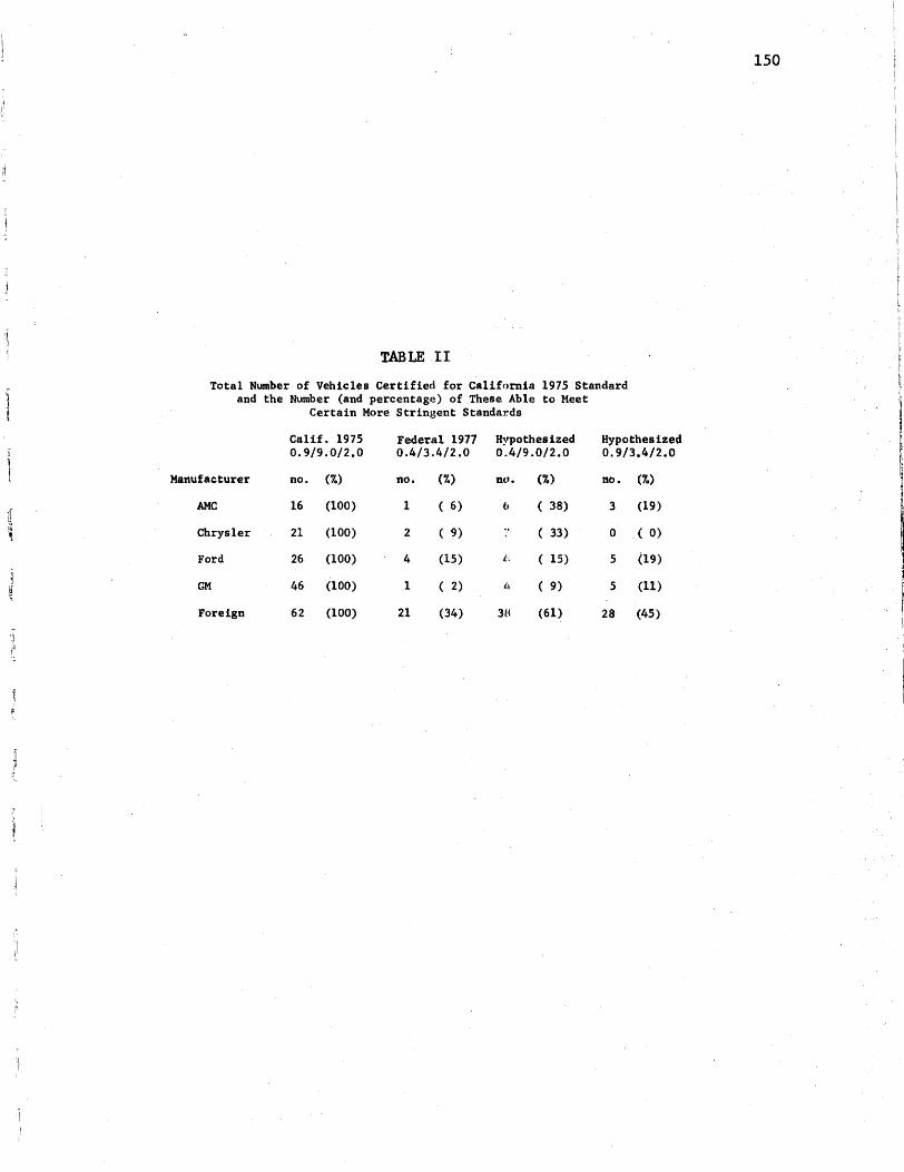


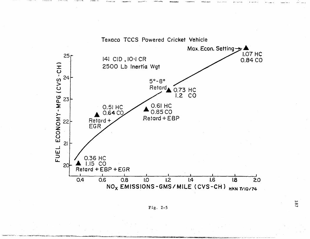


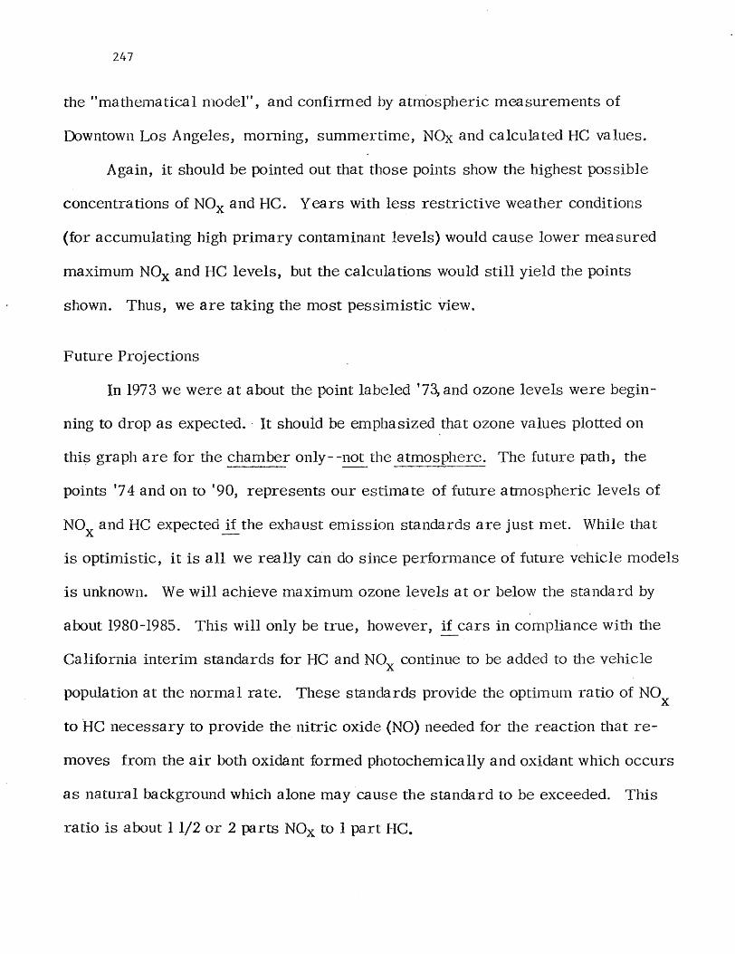


![Malposition and displacement of intrauterine devices ... · IUDs report symptoms [1].The leading conventional T-shape devices such as LNG releasing systems and copper devices have](https://img.dokumen.tips/doc/110x75/5fd903338c72c343d15a6c9c/malposition-and-displacement-of-intrauterine-devices-iuds-report-symptoms-1the.jpg)


![[UIST2013] MagGetz: Customizable Passive TangibleControllers on and around Conventional Mobile Devices](https://img.dokumen.tips/doc/110x75/55a2b9ee1a28ab445f8b45bf/uist2013-maggetz-customizable-passive-tangiblecontrollers-on-and-around-conventional-mobile-devices.jpg)