Embed Size (px)
Citation preview

EM Algorithm
Jur van den Berg

Kalman Filtering vs. Smoothing
• Dynamics and Observation model
• Kalman Filter:– Compute– Real-time, given data so far
• Kalman Smoother:– Compute – Post-processing, given all data
ttt YYX yy ,,| 00
TtYYX TTt 0,,,| 00 yy
),(~
),(~
,
,1
RNV
QNW
C
A
tt
tt
tt
tt
t
t
0v
0w
vx
wx
y
x

EM Algorithm
• Kalman smoother: – Compute distributions X0, …, Xt
given parameters A, C, Q, R, and data y0, …, yt.
• EM Algorithm:– Simultaneously optimize X0, …, Xt and A, C, Q, R
given data y0, …, yt.
),(~
),(~
,
,1
RNV
QNW
C
A
tt
tt
tt
tt
t
t
0v
0w
vx
wx
y
x

Probability vs. Likelihood
• Probability: predict unknown outcomes based on known parameters: – p(x | q)
• Likelihood: estimate unknown parameters based on known outcomes: – L( q | x) = p(x | q)
• Coin-flip example:– q is probability of “heads” (parameter)– x = HHHTTH is outcome

Likelihood for Coin-flip Example
• Probability of outcome given parameter:– p(x = HHHTTH | q = 0.5) = 0.56 = 0.016
• Likelihood of parameter given outcome:– L( q = 0.5 | x = HHHTTH) = p(x | q) = 0.016
• Likelihood maximal when q = 0.6666… • Likelihood function not a probability density

Likelihood for Cont. Distributions
• Six samples {-3, -2, -1, 1, 2, 3} believed to be drawn from some Gaussian N(0, s2)
• Likelihood of s:
• Maximum likelihood:
16.26
321)1()2()3( 222222
)|3()|2()|3(})3,2,1,1,2,3{|( xpxpxpL

Likelihood for Stochastic Model
• Dynamics model
• Suppose xt and yt are given for 0 ≤ t ≤ T, what is likelihood of A, C, Q and R?
• • Compute log-likelihood:
),(~
),(~
,
,1
RNV
QNW
C
A
tt
tt
tt
tt
t
t
0v
0w
vx
wx
y
x
T
ttttt ppRQCApRQCAL
01 )|()|(),,,|,(),|,,,( xyxxyxyx
),,,|,(log RQCAp yx

Log-likelihood
• Multivariate normal distribution N(m, S) has pdf:
• From model:
...)|(log)|(log
)|()|(log),,,|,(log
1
0 01
01
T
t
T
ttttt
T
ttttt
pp
ppRQCAp
xyxx
xyxxyx
),(~1 QAN tt xx ),(~ RCN tt xy
))()(exp()2()( 121
2/112/ μxμxx Tkp
const)()(2
1log2
1
)()(2
1log2
1
1
0
1
11
1
1
0
1
ttT
tt
T
t
ttT
tt
T
t
CRCR
AQAQ
xyxy
xxxx

Log-likelihood #2
• a = Tr(a) if a is scalar• Bring summation inward
...const)()(2
1log2
1
)()(2
1log2
1
1
0
1
11
1
1
0
1
ttT
tt
T
t
ttT
tt
T
t
CRCR
AQAQ
xyxy
xxxx
const))()Tr((2
1log
2
1
))()Tr((2
1log2
0
11
1
01
11
1
T
ttt
Ttt
T
ttt
Ttt
CRCRT
AQAQT
xyxy
xxxx
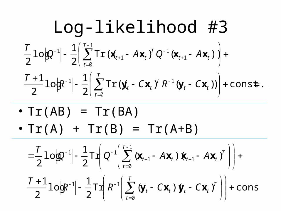
Log-likelihood #3
• Tr(AB) = Tr(BA)• Tr(A) + Tr(B) = Tr(A+B)
...const))()Tr((2
1log
2
1
))()Tr((2
1log2
0
11
1
01
11
1
T
ttt
Ttt
T
ttt
Ttt
CRCRT
AQAQT
xyxy
xxxx
const))((Tr2
1log
2
1
))((Tr2
1log2
0
11
1
011
11
T
t
Ttttt
T
t
Ttttt
CCRRT
AAQQT
xyxy
xxxx

Log-likelihood #4
• Expand
constTr2
1log
2
1
Tr2
1log2
),|,,,(
01
11
1
01111
11
T
t
TTtt
Ttt
TTtt
Ttt
T
t
TTtt
Ttt
TTtt
Ttt
CCCCRRT
AAAAQQT
RQCAl
xxyxxyyy
xxxxxxxx
yx
...const))((Tr2
1log
2
1
))((Tr2
1log2
0
11
1
011
11
T
t
Ttttt
T
t
Ttttt
CCRRT
AAQQT
xyxy
xxxx

Maximize likelihood
• log is monotone function– max log(f(x)) max f(x)
• Maximize l(A, C, Q, R | x, y) in turn for A, C, Q and R.– Solve for A– Solve for C– Solve for Q– Solve for R
0),|,,,(
C
yxRQCAl
0),|,,,(
Q
yxRQCAl
0),|,,,(
R
yxRQCAl
0),|,,,(
A
yxRQCAl

Matrix derivatives
• Defined for scalar functions f : Rn*m -> R
• Key identities
T
TTT
TTT
TTT
AA
A
BA
AB
A
BA
A
AB
AABB
ABB
AAA
log
)(Tr)(Tr)(Tr
)(
)(xx
xx

Optimizing A
• Derivative
• Maximizer
1
01
1 222
1),|,,,( T
t
Ttt
Ttt AQ
A
yxRQCAlxxxx
11
0
1
01
T
t
Ttt
T
t
TttA xxxx

Optimizing C
• Derivative
• Maximizer
T
t
Ttt
Ttt CR
C
yxRQCAl
0
1 222
1),|,,,(xxxy
1
00
T
t
Ttt
T
t
TttC xxxy

Optimizing Q
• Derivative with respect to inverse
• Maximizer
TT
t
TTtt
Ttt
TTtt
Ttt AAAAQ
T
Q
yxRQCAl
1
011111 2
1
2
),|,,,(xxxxxxxx
1
01111
1 T
t
TTtt
Ttt
TTtt
Ttt AAAA
TQ xxxxxxxx

Optimizing R
• Derivative with respect to inverse
• Maximizer
TT
t
TTtt
Ttt
TTtt
Ttt CCCCR
T
R
yxRQCAl
01 2
1
2
1),|,,,(xxyxxyyy
T
t
TTtt
Ttt
TTtt
Ttt CCCC
TR
01
1xxyxxyyy

EM-algorithm
• Initial guesses of A, C, Q, R• Kalman smoother (E-step): – Compute distributions X0, …, XT
given data y0, …, yT and A, C, Q, R.
• Update parameters (M-step):– Update A, C, Q, R such that
expected log-likelihood is maximized• Repeat until convergence (local optimum)
),(~
),(~
,
,1
RNV
QNW
C
A
tt
tt
tt
tt
t
t
0v
0w
vx
wx
y
x

Kalman Smoother• for (t = 0; t < T; ++t) // Kalman filter
• for (t = T – 1; t ≥ 0; --t) // Backward pass
QAAPP
AT
tttt
tttt
||1
||1 ˆˆ xx
ttttttt
tttttttt
Ttt
Tttt
CPKPP
CK
RCCPCPK
|11|11|1
|111|11|1
1
|1|11
ˆˆˆ
xyxx
TtttTttttTt
ttTttttTt
ttT
ttt
LPPLPP
L
PAPL
)(
ˆˆˆˆ
|1|1||
|1|1||
1|1|
xxxx

Update Parameters• Likelihood in terms of x, but only X available
• Likelihood-function linear in • Expected likelihood: replace them with:
• Use maximizers to update A, C, Q and R.
constTr2
1log
2
1
Tr2
1log2
),|,,,(
01
11
1
01111
11
T
t
TTtt
Ttt
TTtt
Ttt
T
t
TTtt
Ttt
TTtt
Ttt
CCCCRRT
AAAAQQT
RQCAl
xxyxxyyy
xxxxxxxx
yx
Ttt
Tttt 1,, xxxxx
TTtttTtTtt
TTttt
Ttt
TTtTtTt
Ttt
Ttt
PLXXE
PXXE
XE
|1|1|1|1|1|1
|||
|
ˆ)ˆˆ(ˆˆ)|(
ˆˆ)|(
ˆ)|(
xxxxxy
xxy
xy
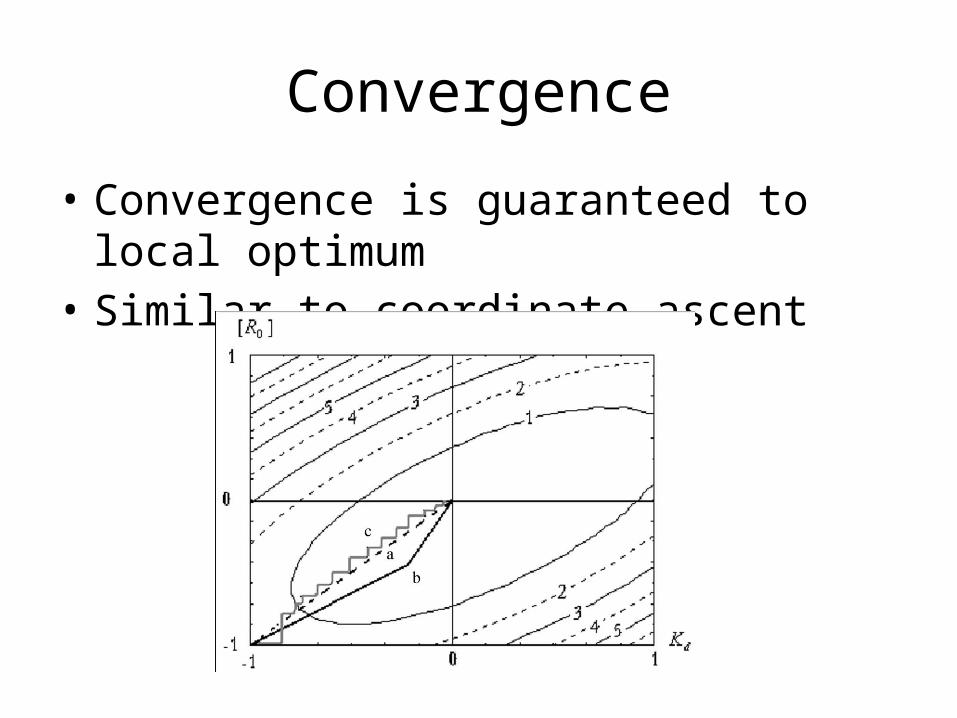
Convergence
• Convergence is guaranteed to local optimum• Similar to coordinate ascent

Conclusion
• EM-algorithm to simultaneously optimize state estimates and model parameters
• Given ``training data’’, EM-algorithm can be used (off-line) to learn the model for subsequent use in (real-time) Kalman filters

Next time
• Learning from demonstrations• Dynamic Time Warping


