Embed Size (px)
Citation preview

Elsevier Editorial System(tm) for Measurement Manuscript Draft Manuscript Number: Title: INTERPRETATION OF THE EXPERIMENTALLY MEASURED DYNAMIC RESPONSE OF AN EMBEDDED RETAINING WALL BY FINITE ELEMENT MODELS Article Type: MetroGeothecnics Papers Keywords: Diaphragm wall, Model refinement, Dynamic properties, System identification. Corresponding Author: Dr. Filippo Santucci de Magistris, PhD Corresponding Author's Institution: University of Molise First Author: Carlo Rainieri Order of Authors: Carlo Rainieri; Arindam Day; Giovanni Fabbrocino, Professor; Filippo Santucci de Magistris, PhD Abstract: Experimental measurements of the ambient vibration response of an embedded retaining wall were used to enhance the understanding of the dynamic behavior of this typology of geotechnical systems. The experimental estimates of the dynamic properties of the soil-wall system made possible the refinement of a numerical model, originally set according to standard geotechnical investigations, by means of sensitivity analyses with respect to a few model parameters. As a result, a representative model of the dynamic behavior of the soil-wall system in operational conditions was obtained. It yielded a significant insight into the soil-structure interaction mechanisms. Under low acceleration field, a superposition principle was validated, resulting in a potential a priori estimation of the response of the overall system based on the knowledge of the decoupled responses of different domains bounded by the excavation and the wall. Suggested Reviewers: Luigi Di Sarno Dipartimento di Ingegneria, University of Sannio [email protected] well-known researcher in Earthquake Engineering Augusto Penna Dipartimento di Ingegneria, University of Sannio [email protected] well-known expert of Earthquake Geotechnical Engineering Giacomo Russo Dipartimento di Ingegneria Civile e Meccanica, University of Cassino and Southern Lazio [email protected] Wee known expert in Geotechnical Engineering

Università degli Studi del Molise Dipartimento di Bioscienze e Territorio
Engineering Division History and Innovation in Constructions
Filippo Santucci de Magistris, Ph.D. [email protected] Tel: +39 0874404935
II Edificio Polifunzionale Via De Sanctis, 86100 Campobasso
Campobasso, 22.06.2015
Dear Prof. Grattan, Dear Guest Editors, please consider the paper “Interpretation of the experimentally measured dynamic
response of an embedded retaining wall by finite element models” by Carlo Rainieri
et al. for possible publication in the special issue MetroGeotechnics of the journal
Measurement.
Regards
Dr. Filippo Santucci de Magistris (Associate Professor of Geotechnical Engineering)
Cover Letter

INTERPRETATION OF THE EXPERIMENTALLY MEASURED DYNAMIC 1
RESPONSE OF AN EMBEDDED RETAINING WALL BY FINITE 2
ELEMENT MODELS 3
4
Carlo Rainieri*1, Arindam Dey#, Giovanni Fabbrocino*2, Filippo Santucci de Magistris*3 5 6
*1Post doctoral Fellow, *2Full Professor, *3Associate Professor 7 Structural and Geotechnical Dynamics Laboratory StreGa 8
Department of Biosciences and Territory, University of Molise 9 Via De Sanctis s.n.c. – 86100 Campobasso (CB), Italy 10
Tel. +39 0874 404883, Fax 0874-404952, 11 Corresponding author’s e-mail: [email protected] 12
13
#Assistant Professor 14 Indian Institute of Technology Guwahati 15
Department of Civil Engineering, Guwahati 781039, 16 Assam, India 17
E-mail: [email protected] 18 19
20
*ManuscriptClick here to view linked References

2/27
1
ABSTRACT 2
Experimental measurements of the ambient vibration response of an embedded retaining wall 3
were used to enhance the understanding of the dynamic behavior of this typology of geotechnical 4
systems. The experimental estimates of the dynamic properties of the soil-wall system made 5
possible the refinement of a numerical model, originally set according to standard geotechnical 6
investigations, by means of sensitivity analyses with respect to a few model parameters. As a result, 7
a representative model of the dynamic behavior of the soil-wall system in operational conditions 8
was obtained. It yielded a significant insight into the soil-structure interaction mechanisms. Under 9
low acceleration field, a superposition principle was validated, resulting in a potential a priori 10
estimation of the response of the overall system based on the knowledge of the decoupled responses 11
of different domains bounded by the excavation and the wall. 12
13 Keywords: Diaphragm wall, Model refinement, Dynamic properties, System identification. 14 15

3/27
1 INTRODUCTION 1
Rigid or flexible retaining walls, such as gravity, cantilever or embedded walls usually support 2
deep excavations, bridge abutments or harbor-quays. The behavior of gravity retaining walls under 3
static conditions is investigated in detail over the years, starting from the rational development of 4
earth pressure theories, which date back to the classical works of Coulomb [1] and Rankine [2]. 5
Their seismic design is also already established and is traditionally based on an extension of 6
Coulomb’s limit equilibrium analysis, commonly known as the Mononobe-Okabe method [3, 4]. 7
The Mononobe-Okabe theory was widely discussed (see, for instance, [5, 6, 7, 8] and the key 8
references listed in [9]) and it is, nowadays, the most common design method among practitioners. 9
It is especially used in the form presented by Seed and Whitman [10], which can be found in many 10
codes and regulations [11, 12, 13]. Notwithstanding the widely accepted use of this method, Ebeling 11
and Morrison [14] asserted: “A small number of model testing programs have filled in some of the 12
blanks in the understanding of dynamic response of retaining -structures. Theoretical studies have 13
been made, but with very limited opportunities to check the results of these calculations against 14
actual, observed behavior. As a result, there are still major gaps in knowledge concerning proper 15
methods for analysis and design”. These words appear to be still valid and particularly appropriate 16
for embedded retaining walls. Under dynamic excitations, the different components of the retaining 17
system exhibit complex and interdependent responses, which can be roughly summarized as 18
follows: 19
(a) dynamic interaction between the wall, the retained backfill and the soil in front of the wall; 20
(b) dynamic interaction of the underlying soil with the sustained structure. 21
These aspects and the effects of damping, natural frequencies of the system, phase lags and 22
amplifications within the backfill on the system response cannot be properly analyzed by means of 23
simplified approaches, such as the Mononobe-Okabe method. 24
Advanced dynamic analysis represents a more refined, but even more complex examination 25
tool. Dynamic analyses by means of finite-difference or finite-element methods can take into 26

4/27
detailed account of the soil-structure interaction, so they are, potentially, the most effective 1
techniques to predict the response of a flexible retaining wall. However, in the absence of 2
systematic studies and criteria for validation of the results provided by such dynamic analyses (for 3
instance, through their correlation to accurate and reliable experimental data), the effectiveness of 4
the tool remains largely dependent on the engineering judgment. 5
Giarlelis and Mylonakis [15] propose a study about the dynamic properties of a cantilever wall. 6
In particular, a Dynamic linear Wall-Soil-Structure Interaction (DWSSI) analysis was carried out to 7
investigate the effect of the presence of the cantilever wall and its flexibility on the induced 8
acceleration of the retained soil. Transfer functions were derived from the acceleration profiles of 9
the wall, allow estimating the natural frequencies of vibration of the system. In any case, simplified 10
geotechnical models in terms of geometry and material properties were considered. Moreover, they 11
do not take advantage of any verification or calibration based on the results of experimental, full 12
scale, in situ dynamic measurements. This limitation can be probably associated to the fairly limited 13
availability of experimental investigations about the dynamics of walls in the literature. Amano et al. 14
[16] execute free and forced full-scale vibration tests on a quay wall in Japan. Fukuoka and 15
Imamura [17] measure earth pressures and accelerations in the case of cantilever, large concrete 16
block and multiple anchored retaining walls during real Japanese earthquakes. Elgamal et al. [18] 17
install a shaker in the backfill of a cantilever retaining wall and analyze the forced vibrations of the 18
system. In any case, all these researches refer to gravity or cantilever walls, while no full-scale data 19
seem to be available about embedded retaining walls. In spite of the research efforts devoted to the 20
analysis of the dynamic response of retaining walls, the above-mentioned references reveal that 21
there is a substantial lack of knowledge about the dynamic properties and response of embedded 22
retaining systems, even in the presence of low amplitude excitations. On the other hand, it is worth 23
noting that results of dynamic analyses heavily depend on the reliability of the model in terms of 24
geometry and input parameters (boundary conditions, material properties, and so on). Thus, 25
extensive geotechnical investigations and the availability of full scale dynamic measurements are 26

5/27
certainly useful for the setting and calibration of effective numerical models of the soil-wall system 1
under operational conditions in view of more sophisticated analyses. 2
The opportunities provided by dynamic measurements on a real embedded retaining wall for 3
the refinement of its numerical model are the main topic of the present paper, which takes into 4
account the above-mentioned technical background and open issues. Herein it is shown, in 5
particular, how the model refinement, founded on the available measurement of the soil-wall natural 6
frequencies, can provide an insight on the most relevant geotechnical parameters affecting the 7
dynamic response of the system under investigation in operational conditions. The paper is 8
organized as follows. Setting of a basic Finite Element (FE) model of the soil-wall system based on 9
data is presented first, and various pertinent issues referring to the main uncertainties in its 10
development are discussed (Section 2 and Section 3). Then, the refinement of the numerical model 11
based on the results of ambient vibration tests is described in detail (Section 4), drawing some 12
interesting conclusions about the soil-structure interaction mechanisms at low amplitude vibrations. 13
2 EXPERIMENTAL CHARACTERIZATION OF THE GEOTECHNICAL SYSTEM 14
The analyzed reinforced concrete (r.c.) embedded retaining wall (Figure 1a) is a part of the 15
new Students’ Residence at the University of Molise in Campobasso, Italy. It consists of two 16
alignments of adjacent but not contiguous piles (Figure 1b). These have a diameter of 800 mm and 17
a length of 18 m. The free height of the wall is 6.4 m. An r.c. beam, whose cross section is 1.0 m 18
high, connects the heads of the piles; there are no anchorages. The herein reported measurements 19
and analyses refer to a time before the construction of the nearby building. 20
Deposits of varicolored scaly stiff clays, with alternate beds of limestone, calcareous marls and 21
sandy materials, and supplementary presence of calcarenite and fragments of San Bartolomeo’s 22
flysch, characterized the site from a geological point of view. The upper layer is constituted by 23
remolded debris cover of anthropogenic origin, whose thickness varies between 4 and 10 m. Figure 24
2a shows the geological map of the area. 25

6/27
(a)
(b)
Figure 1. Picture view of part of the geotechnical works for the New Students’ Residence in 1 Campobasso (a); layout of the equivalent sheet pile cross section, plan view (b) 2
Piles & plate of the building
Top beam
Instrumented piles
H= 6.4 m H= 4.2 m
Retaining wall

(a)
(c) Figure 2. Geological map and section of the Vazzieri 1 clays; ter2 – Deposits of debris cover; 2 Bartolomeo’s Flysch deposit (a); schematic location of boreholes and retaining wall on a contour 3 plot; the general direction of slope in the locality is indicated by the arrow (b); characteristics of 4 strata and SPT test results for Borehole S6 (c) and Borehole S5 (d)5
6
The team of Professional Engineers who designed the Residence according to relevant Italian 7
codes also carried out the geotechnical characterization of the site8
investigations (S5 and S6) performed on both9
7/27
(b)
(d)
Geological map and section of the Vazzieri area in Campobasso. AVS – Varicolored scaly Deposits of debris cover; anf2 – Anthropogenic remolded covering; SAN2
Bartolomeo’s Flysch deposit (a); schematic location of boreholes and retaining wall on a contour general direction of slope in the locality is indicated by the arrow (b); characteristics of
d SPT test results for Borehole S6 (c) and Borehole S5 (d)
team of Professional Engineers who designed the Residence according to relevant Italian
carried out the geotechnical characterization of the site. It was based on two borehole
performed on both sides of the retaining wall. Figure 2b schematically
Varicolored scaly SAN2 – San
Bartolomeo’s Flysch deposit (a); schematic location of boreholes and retaining wall on a contour general direction of slope in the locality is indicated by the arrow (b); characteristics of
team of Professional Engineers who designed the Residence according to relevant Italian
on two borehole
schematically

8/27
shows the positions of the boreholes and the retaining wall. The arrow indicates the general 1
direction of the slope in the investigated area. The borehole investigations were carried out up to a 2
depth of 30 m from the ground level. Stratigraphic Column Extractions, Standard Penetration Tests 3
(SPT) and Down-Hole tests (DH) were executed. Laboratory tests to determine the main physical 4
and mechanical properties of the soil were performed on the extracted samples. The strength 5
parameters of the soil samples were determined by triaxial and direct shear tests. Figure 2c and 6
Figure 2d show the different soil layers, as identified according to the stratigraphical characteristics 7
and the SPT blow counts. Down-hole tests carried out in the two boreholes provided the primary 8
and shear wave velocities (Vp, Vs) profiles. Estimates of the Poisson’s ratio, modulus of elasticity 9
and shear modulus under dynamic conditions were then obtained according to the following well-10
established expressions (see, for instance, Richart et al. [19]): 11
ν =0.5⋅ Vp Vs( )2
−1
Vp Vs( )2−1
; E = γg
⋅Vp2 ⋅
1+ν( ) ⋅ 1− 2ν( )1−ν( )
; G = E
2⋅ 1+ν( ) (1) 12
The variation of the shear wave velocity with depth is reported in Figure 3. 13
As indicated in Figure 2b, since the boreholes are located along the general direction of the 14
slope in the area, there exists a grade difference of about 8 m at the ground level between them. The 15
excavation of the borehole S6 started from an absolute height of about 676 m, while that of 16
borehole S5 commenced from nearly 668 m (Figure 3). The boreholes were separated by a 17
longitudinal distance of about 35 m. Examination of the data has led to recognize the presence of 18
soil layers with nearly identical characteristics but at a certain difference in elevation. An inclined 19
stratigraphy with an approximate slope (1V:10H) was therefore adopted for the geometry of the 20
geotechnical model. This was incorporated in the numerical model of the soil-wall system, which is 21
described in the next section. 22
In order to obtain reference values of the dynamic properties of the wall in view of the 23
refinement of the numerical model, an ambient vibration test was carried out. To this aim it is worth 24
mentioning that two piles of the wall are equipped with six couples of embedded accelerometers, 25

9/27
installed according to two orthogonal directions (parallel to the pile axis and orthogonal to the wall 1
surface) at different positions along the height. Such sensors are part of a permanent seismic 2
monitoring system [20, 21]. 3
4 Figure 3. Shear wave velocity profile obtained from borehole S5 (a) and borehole S6 (b) 5
6
Even if the embedded sensors are able to measure also the ambient vibrations, because they are 7
low-noise, high sensitivity (10 V/g) accelerometers, they are not enough in number to observe the 8
deflection shape of the wall with adequate spatial resolution. Thus, additional five accelerometers 9
with the same characteristics were externally mounted along the free height of the wall. This 10
provided an improvement of the spatial resolution of measurements in the upper part of the wall, 11
which is also characterized by the largest displacements. The additional sensors were equally 12
!
Shear wave velocity Vs (m/s)
Abs
olut
e el
evat
ion
z (m
, am
sl)
Shear wave velocity Vs (m/s)
Abs
olut
e el
evat
ion
z (m
, am
sl)
a)
b)

10/27
spaced at a distance of 0.8 m. Figure 4 shows a picture of the final sensor layout, including the 1
externally mounted as well as the embedded sensors. The horizontal accelerations were therefore 2
measured in eight positions along the height. The ambient vibration response of the wall was 3
acquired for one hour at a sampling rate of 100 Hz. 4
5 Figure 4. Sensor layout 6
7 The ambient vibration response of the wall was analyzed by powerful and robust Operational 8
Modal Analysis (OMA) techniques, such as the Frequency Domain Decomposition (FDD) [22, 23] 9
and the Stochastic Subspace Identification (SSI) [23, 24, 25]. 10

(a)
(c)
Figure 5. Analysis of the ambient vibration response of the1 FDD method (a), stabilization diagram from the SSI method (b), first experimental mode shape (c), 2 second experimental mode shape (d) 3
4
The FDD is a frequency domain, non
based on the Singular Value Decomposition (SVD) of the output Power Spectral Density (PSD)
matrix. Structural resonances are identified from the singular value plots through peak picking; the
corresponding singular vector is a good estimate of the mod
domain, parametric, modal identification procedure based on a state
dynamic problem. The modal parameters are extracted from realizations of the state matrix and
output matrix of the system obtained from measurements of its response to ambient vibrations
through projections and other algebraic operators.
Before processing, data pre-treatment
the absence of errors or anomalies, such as
window and 66% overlap were used for the spectrum computation. A frequency resolution of 0.01
11/27
(b)
(d)
Analysis of the ambient vibration response of the wall: Singular value plots from the FDD method (a), stabilization diagram from the SSI method (b), first experimental mode shape (c),
The FDD is a frequency domain, non-parametric, output-only modal identification techn
based on the Singular Value Decomposition (SVD) of the output Power Spectral Density (PSD)
matrix. Structural resonances are identified from the singular value plots through peak picking; the
corresponding singular vector is a good estimate of the mode shape. The SSI, conversely, is a time
domain, parametric, modal identification procedure based on a state-space description of the
dynamic problem. The modal parameters are extracted from realizations of the state matrix and
btained from measurements of its response to ambient vibrations
and other algebraic operators.
treatment was conducted to validate the quality of the data
the absence of errors or anomalies, such as clipping, drop-out, noise spikes and so on
used for the spectrum computation. A frequency resolution of 0.01
wall: Singular value plots from the FDD method (a), stabilization diagram from the SSI method (b), first experimental mode shape (c),
only modal identification technique
based on the Singular Value Decomposition (SVD) of the output Power Spectral Density (PSD)
matrix. Structural resonances are identified from the singular value plots through peak picking; the
e shape. The SSI, conversely, is a time
space description of the
dynamic problem. The modal parameters are extracted from realizations of the state matrix and
btained from measurements of its response to ambient vibrations
the quality of the data and
noise spikes and so on. Hanning
used for the spectrum computation. A frequency resolution of 0.01
12/27
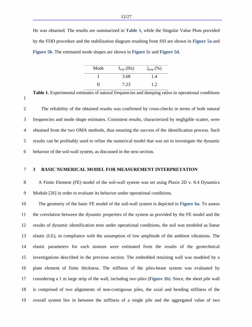
Hz was obtained. The results are summarized in Table 1, while the Singular Value Plots provided
by the FDD procedure and the stabilization diagram resulting from SSI are shown in Figure 5a and
Figure 5b. The estimated mode shapes are shown in Figure 5c and Figure 5d.
Mode fexp (Hz) ξexp (%)
I 3.68 1.4
II 7.23 1.2
Table 1. Experimental estimates of natural frequencies and damping ratios in operational conditions 1
The reliability of the obtained results was confirmed by cross-checks in terms of both natural 2
frequencies and mode shape estimates. Consistent results, characterized by negligible scatter, were 3
obtained from the two OMA methods, thus ensuring the success of the identification process. Such 4
results can be profitably used to refine the numerical model that was set to investigate the dynamic 5
behavior of the soil-wall system, as discussed in the next section. 6
3 BASIC NUMERICAL MODEL FOR MEASUREMENT INTERPRETATION 7
A Finite Element (FE) model of the soil-wall system was set using Plaxis 2D v. 8.4 Dynamics 8
Module [26] in order to evaluate its behavior under operational conditions. 9
The geometry of the basic FE model of the soil-wall system is depicted in Figure 6a. To assess 10
the correlation between the dynamic properties of the system as provided by the FE model and the 11
results of dynamic identification tests under operational conditions, the soil was modeled as linear 12
elastic (LE), in compliance with the assumption of low amplitude of the ambient vibrations. The 13
elastic parameters for each stratum were estimated from the results of the geotechnical 14
investigations described in the previous section. The embedded retaining wall was modeled by a 15
plate element of finite thickness. The stiffness of the piles-beam system was evaluated by 16
considering a 1 m large strip of the wall, including two piles (Figure 1b). Since, the sheet pile wall 17
is comprised of two alignments of non-contiguous piles, the axial and bending stiffness of the 18
overall system lies in between the stiffness of a single pile and the aggregated value of two 19

contiguous piles connected by the top be1
(EA) = 3.08x10⁷ kN/m, and bending stiffness (2
the plate element (deq) is evaluated by the following expression: 3
1.362 m was adopted for the same in the model. 4
soil-wall interface. The water table was5
investigations. Table 2 summarizes the adopted soil and wall parameters for the 6
(a)
(c)
(e)
7 Figure 6. Views of the FE models in the region around the wall: 8 (a) and its zoomed meshing (b); zoomed view of the 9 (c) and its meshing (d); zoomed view of the 10 its meshing (f) 11
12
13
Soil
Layer Material
Type E0
(105 kPa)
G0
(105 kPa)
A LE 3.188 1.113
B LE 4.086 1.433 C LE 14.51 5.045
D LE 26.49 9.243 Table 2. Material properties of soil adopted in the basic FE model14
13/27
top beam. The adopted scaled down values are: axial stiffness
ending stiffness (EI) = 4.76x10⁶ kNm2/m. The equivalent thickness of
) is evaluated by the following expression: deq=12 ∗ /, and a value of
adopted for the same in the model. A no-slip debonding condition was assume
was below the model, as resulting from the geotechnical
the adopted soil and wall parameters for the basic model.
(b)
(d)
(f)
Views of the FE models in the region around the wall: Geometry of the basic zoomed view of the FE model geometry after the first refinement
zoomed view of the FE model geometry after the second refinement (e) and
kPa) ν
γ
(kN/m3)
Vs
(m/s)
HL (m)
Left of wall
H
Right of Wall
0.432 18.00 246.2 8
0.426 19.03 271.6 3 0.438 19.47 503.9 5
0.433 19.98 673.3 10 Material properties of soil adopted in the basic FE model
xial stiffness
/m. The equivalent thickness of
, and a value of
assumed at the
geotechnical
model.
Geometry of the basic FE model geometry after the first refinement
eometry after the second refinement (e) and
HR (m)
Right of Wall
3
3 5
10

14/27
Before the evaluation of the correlation between numerical and experimental results, the model 1
was optimized in order to obtain its best functionality. A basic guidance to the selection of 2
appropriate numerical parameters, so that the reliability and accuracy of the predictions are not 3
jeopardized, is reported in the following. Further suggestions about analysis parameter settings are 4
given in [26]. 5
A fairly accurate model was set in compliance with appropriate guidelines reported in the 6
literature and proved by the results of a series of dynamic analyses of vertical propagation of S-7
waves in an homogeneous layer using Plaxis 2D v. 8.4 Dynamic module [27]. Those approaches 8
allow to properly account for the influence of boundary conditions, meshing and damping 9
parameters on the response of the system A domain aspect ratio of 40 (ratio of total domain width to 10
the average height) was chosen, after a trial and error procedure to fulfill the assumption of semi-11
infinite soil. 12
Absorbent boundaries were used setting the relaxation coefficients as follows: C1=1 and 13
C2=0.25 [28]. 14
The criteria reported in [29] were adopted to determine the mesh size, and a suitable refined 15
meshing scheme was accordingly set. Figure 6b portrays the adopted meshing for the mentioned 16
numerical model. 17
In order to extract the dynamic properties of the model of the soil-wall system, a Gaussian 18
white noise (duration: 1 hour; sampling frequency: 100 Hz) and an impulse load were alternatively 19
applied as input, so that all the modes in the frequency range of interest were almost equally excited 20
[30]. The excitation was applied as propagating shear waves generated by base shaking and a 21
dynamic analysis of the basic model was carried out to determine the acceleration responses of the 22
retaining wall at different locations, corresponding to the positions of the sensors in the 23
experimental tests. Numerical damping parameters [31, 32] affect the amplification of the response 24
at resonances but not the shape of the amplification function. An implicit Newmark scheme governs 25
the numerical time-integration and Newmark damping parameters specifies numerical damping. An 26

15/27
Undamped Newmark Scheme, also known as average acceleration scheme, was considered (so that 1
the predicted frequency spectra suffer minimal effect from numerical damping) with the following 2
parameters: Nα=0.25 and Nβ=0.5. Rayleigh damping is used to simulate material damping under 3
plane-strain conditions. Rayleigh parameters were determined following the Park and Hashash 4
approach [33]. Considering a 1% damping on the overall system in agreement with the 5
experimental estimates (Table 1), Rayleigh damping parameters were set as follows: Rα=0.293 and 6
Rβ=3.032E-4, both for the soil and the wall. The fundamental dynamic properties of the model were 7
then extracted by conventional input-output dynamic identification techniques [34], such as the 8
deterministic subspace identification [23]. The dynamic properties of the modeled system were 9
finally compared with the corresponding experimental estimates obtained from field dynamic 10
measurements. The values of the fundamental resonant frequencies of the basic numerical model of 11
the wall were equal to 4.7 Hz and 6.7 Hz, respectively. Since these values were slightly different 12
from the corresponding experimental estimates, as reported in Table 3, a refinement of the FE 13
model to more closely match the experimental results was needed. The process for minimization of 14
the scatter between experimental observations and numerical predictions is described in detail in the 15
next section. 16
17 Basic model
Mode fexp (Hz) fFEM (Hz) Scatter (%)
I 3.68 4.7 21.7
II 7.23 6.7 -7.33
First refinement
Mode fexp (Hz) fFEM (Hz) Scatter (%)
I 3.68 3.64 -1.1
II 7.23 7.46 3.1
Table 3. Comparisons between experimental and numerical estimates of the natural frequencies: the 18 basic FE model and the FE model after the first refinement 19 20 21 22

16/27
4 MODEL REFINEMENT 1
4.1 SELECTION OF THE UPDATING PARAMETERS 2
Modification of the model parameters and assumptions can be carried out to minimize 3
discrepancies between numerical predictions and experimental results. A classical approach in this 4
direction would be a trial-and-error scheme; however, when it is mostly governed by the random 5
changes in the contributory factors, it is highly tedious, time-consuming and often based on 6
intuitions rather than justified by a mathematical and logical approach. As alternatives, some robust 7
computational procedures were developed over time, to achieve the same in a regularized manner. 8
In particular, experimental estimates of dynamic properties (natural frequencies and mode shapes) 9
are being largely used for model parameter adjustments, especially in the field of structural 10
engineering. A detailed discussion about model updating procedures and some applications can be 11
found elsewhere [35, 36]. 12
In this section, the main uncertainties affecting the numerical model of the soil-wall system are 13
identified and the process for the minimization, in a regularized manner, of the scatter with the 14
reference experimental results is described. In particular, the model refinement aimed at optimizing 15
the correlation with the experimental results, quantified by the frequency scatter: 16
∆f =fi,FEM − fi,exp
fi,exp
⋅100 i=1, 2 (2) 17
(where fi,FEM and fi,exp are the numerical and experimental value of the natural frequency of the 18
i-th mode, respectively) and the mode shape correlation expressed by the MAC index [37]: 19
MAC φi,FEM , φi,exp ( ) =φi,FEM T φi,exp
2
φi,FEM T φi,FEM ( ) φi,exp T φi,exp ( )i =1,2. (3) 20
φi,FEM and φi,exp are the numerical and experimental mode shape vectors for the i-th mode, 21
respectively; the superscript T denotes transpose. 22

17/27
Regarding the uncertainties in the model geometry, it is worth noting that the above-mentioned 1
boreholes, S5 and S6, each 30 m deep, though allow for a reasonable identification of the soil 2
stratigraphy for design purposes, do not provide enough insight about the depth and profile of the 3
bedrock. However, its location has significant influence on the dynamic response of the model. 4
Since most of the model parameters are directly measured from in-situ and laboratory tests on soil, 5
the indirect identification of the bedrock depth and profile was selected as a target of the refinement 6
process. Sensitivity analyses showed that the results are fairly dependent to these parameters, which 7
are, at the same time, the most uncertain, as pointed out also by the results of SPT tests. In fact, SPT 8
blow-counts of boreholes S5 and S6 reveal a refusal of penetration at 20 m and 26 m, but, the 9
borehole is excavated further until 30 m. Hence, it is very difficult to adjudge the soil at this depth 10
to be or not as a part of the bedrock. Moreover, results from the two borehole investigations are 11
actually not sufficient to describe the global profile of the substrata along the direction orthogonal 12
to the wall; as a consequence the boreholes provide only a glimpse of the local stratigraphy. On the 13
contrary, the dynamic response of the soil-wall system is definitely affected by the substrata profile. 14
For further clarification about soil geometry, borehole investigations in the nearby vicinity of the 15
study-area were also inspected. They seem to show the presence of hard soils on the excavated side 16
at a depth of about 15 m, as depicted in Figure 7, but there is no evidence of the presence of the 17
bedrock. Even less information is available about the soil behind the wall, due to a lack of 18
investigative explorations. The already mentioned borehole S6 provides the only instance. Since 19
there is a lack of information and a significant grade difference between the stratigraphic profile of 20
the soils in the back and in front of the wall, it is quite difficult to verify the depth of the bedrock, in 21
particular on the backfill side, or adjudge the irregularity in the profile of the bedrock across the 22
transverse direction of the wall according only to the results of in-situ investigations. 23

18/27
1
Figure 7. Conglomerated plot of SPT blow-counts from the nearby boreholes towards the soil in 2 front of the wall as a function of depth from the ground level 3
4
As a consequence, the refinement process had the identification of the depth and the profile of 5
the bedrock as a primary concern. After that, minor refinements were obtained by properly setting 6
the elastic parameters of the two upper layers on the backfill side of the wall. In fact, inspection of 7
Figure 3 points out also that the shear wave profile from borehole S6 is more scattered than the 8
same from S5, especially within 16 m from the ground level. Taking into account that the rotation 9
of the wall due to excavation also implies a slight stiffness reduction of the soil in the upper part of 10
the backfill side of the wall, the effect of the change of stiffness of the different layers in the ranges 11
obtained from the DH tests in S6 was also investigated, leading to a finer refinement of the 12
numerical model. 13
14
4.2 MODEL REFINEMENT FROM ANALYSIS OF THE INTERACTION AMONG THE 15
GEOLOGICAL FORMATIONS 16
The analysis of the model geometry reveals that the retaining wall actually represents a 17
boundary between the two halves of the system. It separates the geological formation in two 18
Number of SPT blows (N)
Dep
th f
rom
the
gro
und
leve
l y (m
)
19/27
domains having a significant grade difference of about 8 m. The two domains of the system, if 1
separately analyzed, show different dynamic properties. 2
The retaining wall, located at the boundary, depicts influences from both the domains, roughly 3
represented by a superposition of the frequency responses of the two previously mentioned parts. In 4
order to study the influence of the two domains, the spectral responses of the free-field motions in 5
each of the areas are studied and compared to the overall response of the system. Considering the 6
basic model, trials with different thickness of the bottom-most layer are carried out in order to get a 7
better insight into the issue. 8
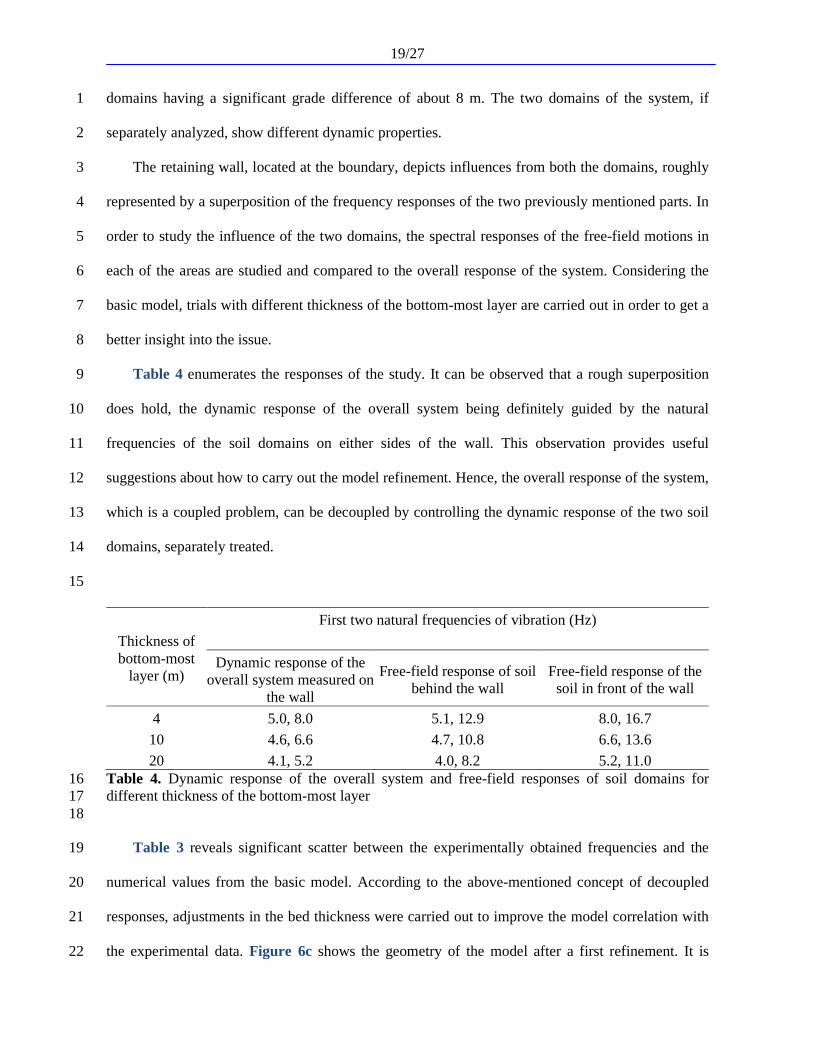
Table 4 enumerates the responses of the study. It can be observed that a rough superposition 9
does hold, the dynamic response of the overall system being definitely guided by the natural 10
frequencies of the soil domains on either sides of the wall. This observation provides useful 11
suggestions about how to carry out the model refinement. Hence, the overall response of the system, 12
which is a coupled problem, can be decoupled by controlling the dynamic response of the two soil 13
domains, separately treated. 14
15
Thickness of bottom-most
layer (m)
First two natural frequencies of vibration (Hz)
Dynamic response of the overall system measured on
the wall
Free-field response of soil behind the wall
Free-field response of the soil in front of the wall
4 5.0, 8.0 5.1, 12.9 8.0, 16.7
10 4.6, 6.6 4.7, 10.8 6.6, 13.6
20 4.1, 5.2 4.0, 8.2 5.2, 11.0 Table 4. Dynamic response of the overall system and free-field responses of soil domains for 16 different thickness of the bottom-most layer 17
18
Table 3 reveals significant scatter between the experimentally obtained frequencies and the 19
numerical values from the basic model. According to the above-mentioned concept of decoupled 20
responses, adjustments in the bed thickness were carried out to improve the model correlation with 21
the experimental data. Figure 6c shows the geometry of the model after a first refinement. It is 22

20/27
characterized by thicker bed at the left of the wall and a comparatively thinner bed on its right, in 1
agreement with the presence of hard soil recognized during the in-situ investigations. The 2
connection between the two beds governs the actual dynamic superposition effect on the wall, and it 3
was chosen by trial and guided by the frequency scatter. Figure 6d portrays the meshing of the 4
adopted model; Table 5 enumerates the material properties of the best model after the first 5
refinement. 6
Table 3 also delivers a comparison between the dynamic properties obtained from the 7
experimental investigations and the numerical predictions after the first refinement. The refined 8
model has, therefore, provided results characterized by reduced frequency scatter, and as such it 9
could be referred to as fairly representative of the actual behavior of the system in operational 10
conditions. However, scrutiny of mode shapes revealed a reversal of the modes obtained from the 11
numerical model with respect to those provided by ambient vibration tests. In fact, the highest MAC 12
values were located on the anti-diagonal of the 2-by-2 MAC matrix between the experimental and 13
numerical mode shapes. 14
15
First refinement
Soil
Layer Material
Type E0L
(105 kPa)
E0R
(105 kPa) ν
γ
(kN/m3)
HL (m)
HR (m)
A LE 1.704 3.188 0.432 18.00 8 3
B LE 2.930 4.086 0.426 19.03 3 3 C LE 14.86 14.51 0.438 19.47 5 5
D LE 26.49 26.49 0.433 19.98 20 4
Second refinement
Soil Layer
Material Type
E0L (105 kPa)
E0R (105 kPa)
ν γ
(kN/m3) HL (m)
HR (m)
A LE 1.565 3.188 0.432 18.00 8 3 B LE 3.482 4.086 0.426 19.03 3 3
C LE 14.86 14.51 0.438 19.47 5 5 D LE 26.49 26.49 0.433 19.98 19 35
Table 5. Material properties adopted in the FE model after the first and second refinement (L= left 16 side of the wall), (R= right side of the wall) 17 18

21/27
The observed inversion depended on the chosen geometry of the model. The initial choice was 1
guided by the presence of hard soil on the excavated side at a depth of about 15 m. Another 2
refinement to the model was carried out wherein the thickness of the base layer on the left side is 3
less in comparison to the right side, and hence, the connection in the base layer is downward 4
sloping from left to right. Figure 6e reports the geometry of the model, while the adopted meshing 5
is portrayed in Figure 6f. Table 5 provides the material properties adopted in the model after the 6
second refinement. 7
Table 6 shows the comparison of the dynamic properties obtained from the model after the 8
second refinement and the corresponding experimental estimates. The scatter in terms of 9
frequencies was substantially reduced with respect to the basic model (Table 3) and the correlation 10
was improved also in comparison to the first refined model (Table 3). In particular, the results 11
reported in Table 3 and Table 6 represent the best correlation as provided by sensitivity analyses 12
with respect to the updating parameters, including the elastic properties of the two upper layers in 13
the backfill side of the wall. A little stiffness decrease with respect to the corresponding layers on 14
the excavated side was required to optimize the correlation. After the second refinement, the mode 15
inversion was no more observed and a high correlation between numerical and experimental mode 16
shapes, pointed out by MAC values very close to 1 (Table 6), was obtained. 17
18 Mode fexp (Hz) fFEM (Hz) Scatter (%) MAC
I 3.68 3.65 -0.81 0.994
II 7.23 7.32 1.24 0.997
Table 6. Correlation between experimental and numerical estimates of the dynamic properties: FE 19 model after the second refinement 20
5 CONCLUSIONS 21
The dynamic response of embedded retaining walls is not frequently investigated in 22
geotechnical engineering. However, the recent seismic events in urban areas dredged out the 23
necessity to enhance the knowledge about the dynamic behavior of such structures. 24

22/27
The present paper discussed about the use of the measurements of the natural frequencies and 1
the modal shapes of an embedded retaining wall to get a representative model of in operational 2
conditions after a process of refinement. According to the results of geotechnical investigations, a 3
basic numerical model was set and its dynamic response was analyzed. The main sources of 4
uncertainty were identified and the numerical model was refined by optimizing the correlation 5
between experimental and numerical estimates of the dynamic properties of the soil-wall system. 6
The resulting model can be, therefore, referred to as representative of the real system in its 7
operational conditions. The mutual influence of retained and excavated side of the wall was 8
documented and a superposition principle accordingly validated, resulting in a potential a priori 9
estimation of the response of the overall system based on the knowledge of the decoupled responses 10
of different domains defined by the excavation. 11
The results of the study are certainly promising and encouraging in view of their extension to 12
the simulation of the response of the system under seismic excitation through the adoption of more 13
advanced soil constitutive models and taking advantage of measurements of the wall response to 14
eventual ground motions occurring in the area. 15
16
ACKNOWLEDGMENTS 17
The present research was partially supported by the ReLuis-DPC Executive Project 2014-2016, 18
Special Project “Monitoring”, whose contribution is gratefully acknowledged. Support of the 2008 19
Italian Ministry of Education “Indian-fellowship” program and the University of Molise to Dr. 20
Dey’s post-doc research fellowship is also gratefully acknowledged. 21
22 REFERENCES 23 24
[1] Coulomb, C.A. (1776). “Essai sur une application des regles des maximis et minimis a 25
quelques problemes de statique relatifs a l'architecture”. Memoires de l'Academie Royale 26
pres Divers Savants, 7. 27

23/27
[2] Rankine, W. (1857). “On the stability of loose earth”. Philosophical Transactions of the 1
Royal Society of London, 147. 2
[3] Okabe, S. (1926). “General theory of earth pressures”, Journal of the Japan Society of Civil 3
Engineering, 12(1). 4
[4] Mononobe, N. and Matsuo, H. (1929). “On the determination of earth pressure during 5
earthquakes”. Proceedings of the World Engineering Conference, Vol. 9, Tokyo, Japan, 6
177-185. 7
[5] Veletsos, A.S. and Younan, A.H. (1997). “Dynamic response of cantilever retaining walls”. 8
ASCE Journal of Geotechnical and Geoenvironmental Engineering, 123(2), 161–172. 9
[6] Koseki, J., Tatsuoka, F., Munaf, Y., Tateyama, M. and Kojima, K. (1997). “A modified 10
procedure to evaluate active earth pressure at high seismic loads”. Soils and Foundations, 11
Special Issue on Geotechnical Aspects of the January 17 1995 Hyogoken-Nambu 12
Earthquake, 209-216. 13
[7] Nakamura, S. (2006). “Reexamination of Mononobe-Okabe theory of gravity retaining walls 14
using centrifuge model tests”. Soils and Foundations, 46(3), 135-146. 15
[8] Mylonakis, G., Kloukinas, P. and Papantonopoulos, C. (2007). “An alternative to the 16
Mononobe–Okabe equations for seismic earth pressures”. Soil Dynamics and Earthquake 17
Engineering, 27(10), 957–969. 18
[9] NCHRP - National Cooperative Highway Research Program (2008). “Seismic Analysis and 19
Design of Retaining Walls, Buried Structures, Slopes, and Embankments”. Transportation 20
Research Board, Report 611, pp. 137. 21
[10] Seed, H.B. and Whitman, R.V. (1970). “Design of earth retaining structures for dynamic 22
loads”. Proceedings of Specialty Conference on Lateral Stresses in the Ground and Design 23
of Earth Retaining Structures, American Society of Civil Engineers, Ithaca, New York, 24
USA, 103-147. 25
[11] EN 1998-5 - Eurocode 8 Part 5 (2003). “Design of structures for earthquake resistance – 26
Part 5: Foundations, retaining structures and geotechnical aspects”. CEN European 27
Committee for Standardization, Bruxelles, Belgium. 28
[12] NTC (2008). “Nuove Norme Tecniche per le Costruzioni”, D.M. Infrastrutture 14/01/2008, 29
Consiglio Superiore dei Lavori Pubblici, published on S.O. n. 30 at the G.U. 04/02/2008 n. 30
29 (in Italian). 31
[13] FEMA - Federal Emergency Management Agency (2009). “NEHRP Recommended Seismic 32
Provisions for Seismic Regulation of Buildings and Other Structures”, FEMA P-750, 33

24/27
prepared for FEMA by the Building Seismic Safety Council. Federal Emergency. 1
Management Agency, Washington, D.C. 2
[14] Ebeling, R.M. and Morrison, E.E. (1992). “The Seismic Design of Waterfront Retaining 3
Structures”. Technical Report ITL-92-11. Vicksburg, Mississippi: Corps of Engineers 4
Waterways Experiment Station. 5
[15] Giarlelis, C. and Mylonakis, G. (2011). “Interpretation of dynamic retaining wall model 6
tests in light of elastic and plastic solutions”. Soil Dynamics and Earthquake Engineering, 7
31(1), 16-24. 8
[16] Amano, R., Azuma, H. and Ishii, Y. (1956). “Aseismic Design of Quay Walls in Japan”. 9
Proceedings of The First World Conference on Earthquake Engineering, Berkeley, 10
California, pp. 32-1, 32-17. 11
[17] Fukuoka, M. and Imamura, Y. (1985). “Researches on retaining walls during earthquake”. 12
Proceedings of The 8th World Conference on Earthquake Engineering, Vol. 3, San 13
Francisco, CA, USA, 501-508. 14
[18] Elgamal, A.-W., Alampalli, S. and Van Laak, P. (1996). “Forced Vibration of Full‐Scale 15
Wall Backfill System”. ASCE Journal of Geotechnical and Geoenvironmental Engineering, 16
122(10), 849-858. 17
[19] Richart, F.E., Hall, J.R. and Woods, R.D. (1970). “Vibrations of soils and foundations”, 18
Prentice-Hall, Englewood Cliff, New Jersey. 19
[20] Fabbrocino, G., Laorenza, C., Rainieri, C. and Santucci de Magistris, F. (2009). “Seismic 20
monitoring of structural and geotechnical integrated systems”. Materials Forum, 33, 404-21
419. 22
[21] Rainieri, C., Fabbrocino, G. and Santucci de Magistris, F. (2013). “An integrated seismic 23
monitoring system for a full- scale embedded retaining wall”. GeotechnicalTesting Journal, 24
36(1), 1–15. 25
[22] Brincker, R., Zhang, L. and Andersen, P. (2001). “Modal identification of output-only 26
systems using frequency domain decomposition”. Smart Materials and Structures, 10, 441-27
445. 28
[23] Rainieri, C. and Fabbrocino, G. (2014). “Operational Modal Analysis of Civil Engineering 29
Structures: An Introduction and Guide for Applications”, Springer, New York. 30
[24] Van Overschee, P. and De Moor, B. (1996). “Subspace identification for linear systems: 31
Theory – Implementation – Applications”, Kluwer Academic Publishers, Dordrecht, The 32
Netherlands. 33

25/27
[25] Peeters B. (2000). “System identification and damage detection in civil engineering”, Ph.D. 1
Thesis, Katholieke Universiteit Leuven, Leuven, Belgium. 2
[26] Brinkgreve, R.B. (2002). “Plaxis 2D Version 8.4: Reference, Scientific and Dynamics 3
Manuals”, Balkema, Lisse, The Netherlands. 4
[27] Visone, C., Bilotta, E. and Santucci de Magistris, F. (2010). “One-dimensional ground 5
response as a preliminary tool for dynamic analyses in Earthquake Geotechnical 6
Engineering”. Journal of Earthquake Engineering. 14(1), 131 – 162. 7
8
[28] Lysmer, J. and Kuhlemeyer, R.L. (1969). “Finite dynamic model for infinite media”. Journal 9
of Engineering Mechanics Division Proceedings ASCE 95(EM4), 859-877. 10
[29] Kuhlemeyer, R.L. and Lysmer, J. (1973). “Finite element method accuracy for wave 11
propagation problems”. Journal of the Soil Mechanics and Foundations Division 12
Proceedings ASCE 99(SM5), 421-427. 13
[30] Bendat, J.S. and Piersol, A.G. (2000). “Random data: analysis and measurement 14
procedures”, 3rd edn., John Wiley & Sons, New York, USA. 15
[31] Barrios, D.B., Angelo, E. and Goncalves, E. (2005). “Finite element shot peening simulation 16
for residual stress analysis and comparison with experimental results”. Mecànica 17
Computacional, 3(XXIV), 413-422. 18
[32] LUSAS (2000). “Theory Manual”, FEA Ltd, United Kingdom. 19
[33] Park, D. and Hashash, Y.M. (2004). “Soil damping formulation in nonlinear time domain 20
site response analysis”. Journal of Earthquake Engineering, 8(2), 249-274. 21
[34] Ewins, D.J. (2000). “Modal Testing: Theory, Practice and Application”, 2nd edn. Research 22
Studies Press Ltd., Baldock. 23
[35] Friswell, M.I. and Mottershead, J.E. (1995). “Finite Element Model Updating in Structural 24
Dynamics”, Kluwer Academic Publishers, Dordrecht, The Netherlands. 25
[36] Mottershead, J.E., Link, M. and Friswell, M.I. (2010). “The sensitivity method in finite 26
element model updating: A tutorial”. Mechanical Systems and Signal Processing, 25(7), 27
2275-2296. 28
[37] Allemang, R.J. and Brown, D.L. (1982). “A correlation coefficient for modal vector 29
analysis”. Proceedings of the 1st SEM International Modal Analysis Conference, Orlando, 30
FL, USA. 31
32

26/27
List of Figures 1
Figure 1 Picture view of part of the geotechnical works for the New Students’ Residence in Campobasso (a); layout of the equivalent sheet pile cross section, plan view (b)
Figure 2 Geological map and section of the Vazzieri area in Campobasso. AVS – Varicolored scaly clays; ter2 – Deposits of debris cover; anf2 – Anthropogenic remolded covering; SAN2 – San Bartolomeo’s Flysch deposit (a); schematic location of boreholes and retaining wall on a contour plot; the general direction of slope in the locality is indicated by the arrow (b); characteristics of strata and SPT test results for Borehole S6 (c) and Borehole S5 (d)
Figure 3 Shear wave velocity profile obtained from borehole S5 (a) and borehole S6 (b)
Figure 4 Sensor layout
Figure 5 Analysis of the ambient vibration response of the wall: Singular value plots from the FDD method (a), stabilization diagram from the SSI method (b), first experimental mode shape (c), second experimental mode shape (d)
Figure 6 Views of the FE models in the region around the wall: Geometry of the basic FE model (a) and its zoomed meshing (b); zoomed view of the FE model geometry after the first refinement (c) and its meshing (d); zoomed view of the FE model geometry after the second refinement (e) and its meshing (f)
Figure 7 Conglomerated plot of SPT blow-counts from the nearby boreholes towards the soil in front of the wall as a function of depth from the ground level
2 3

27/27
List of Tables 1
2
Table 1 Experimental estimates of natural frequencies and damping ratios in operational conditions
Table 2 Material properties of soil adopted in the basic FE model
Table 3 Comparisons between experimental and numerical estimates of the natural frequencies: the basic FE model and the FE model after the first refinement
Table 4 Dynamic response of the overall system and free-field responses of soil domains for different thickness of the bottom-most layer
Table 5 Material properties adopted in the FE model after the first and second refinement (L= left side of the wall), (R= right side of the wall)
Table 6 Correlation between experimental and numerical estimates of the dynamic properties: FE model after the second refinement