REVIEW

ELM-based gene expression classification with misclassificationcost

Hui-juan Lu • En-hui Zheng • Yi Lu •

Xiao-ping Ma • Jin-yong Liu

Received: 24 February 2013 / Accepted: 24 October 2013

� Springer-Verlag London 2013

Abstract Cost-sensitive learning is a crucial problem in

machine learning research. Traditional classification prob-

lem assumes that the misclassification for each category

has the same cost, and the target of learning algorithm is to

minimize the expected error rate. In cost-sensitive learning,

costs of misclassification for samples of different catego-

ries are not the same; the target of algorithm is to minimize

the sum of misclassification cost. Cost-sensitive learning

can meet the actual demand of real-life classification

problems, such as medical diagnosis, financial projections,

and so on. Due to fast learning speed and perfect perfor-

mance, extreme learning machine (ELM) has become one

of the best classification algorithms, while voting based on

extreme learning machine (V-ELM) makes classification

results more accurate and stable. However, V-ELM and

some other versions of ELM are all based on the

assumption that all misclassifications have same cost.

Therefore, they cannot solve cost-sensitive problems well.

To overcome the drawback of ELMs mentioned above, an

algorithm called cost-sensitive ELM (CS-ELM) is

proposed by introducing misclassification cost of each

sample into V-ELM. Experimental results on gene

expression data show that CS-ELM is effective in reducing

misclassification cost.

Keywords Extreme learning machine �Classification accuracy � Misclassification cost

1 Introduction

In the field of classification, cost-sensitive problem has

been a hot topic for a long time and has attracted many

researchers’ attention [1–7]. The popular classifiers that

widely used are SVM, BP, extreme learning machine

(ELM), and so on. Minority of the popular classifiers, such

as ELM, support vector machine [2, 7], neural network and

bayesian decision tree are all based on ‘‘0–1’’ loss [8].

Thus, these classification algorithms imply the following

hypothesis: Misclassification cost for each sample is the

same. However, in practical applications, such as in med-

ical diagnosis, fraud detection, fault diagnosis, the

hypothesis does not apply. For example, in medical diag-

nosis, the cost that someone who has a life-threatening

disease is mistakenly diagnosed as a healthy person is not

equal to the cost that a healthy person is mistakenly diag-

nosed as a diseased person. The former takes the patient’s

deteriorated health status, even death as cost, while the

latter takes side effects of the drug or treatment as cost.

This means that the former is obviously far more severe

than the latter. In those cases, reducing the cost of decision

and improving the classification reliability are both extre-

mely important. Cost-sensitive machine learning (CML)

algorithms were proposed by introducing the asymmetric

misclassification cost into machine learning algorithms.

H. Lu (&)

College of Information Engineering, China Jiliang University,

Hangzhou 310018, China

e-mail: hjlu@cjlu.edu.cn; huijuanlu29@gmail.com

H. Lu � X. Ma

School of Information and Electric Engineering, China

University of Mining and Technology, Xuzhou 221008, China

E. Zheng � J. Liu

College of Mechanical and Electric Engineering, China Jiliang

University, Hangzhou 310018, China

Y. Lu

Department of Computer Science, Prairie View A&M

University, Prairie View, TX 77446, USA

123

Neural Comput & Applic

DOI 10.1007/s00521-013-1512-x

CML is one of the important topics in machine learning,

whose objective is to minimize the average misclassifi-

cation cost rather than maximize classification accuracy.

CML can be realized by sampling methods and modifying

algorithms.

The sampling methods improve the classification accu-

racy by reconstructing classifiers for small class samples,

which have larger misclassification cost. Kubat [9] pro-

posed a representative under-sampling method to delete

noise samples, samples at the boundary, and samples in the

redundant classes. It is effective while the distribution ratio

is less than 70. Bagging and multiple classifiers improve

the accuracy of the classifier by ensemble of two trained

under-sampling methods, thus reducing the average mis-

classification cost [10]. Different from under-sampling,

over-sampling method copies or interpolates minority

classes to reduce the unbalance degree of dataset [11].

Japkowicz [12] evaluated the over-sampling and under-

sampling methods on unbalanced data and showed that

both kinds of methods are effective. Based on the different

misclassification cost of samples, Elkan [13] assigned the

samples with different weights and further reconstructed

the trained datasets. Zhou [14] designed the under-sam-

pling and over-sampling algorithm, where the distribution

of training dataset depends on the misclassification cost of

various classes. Based on under-sampling technique, Liu

[15] proposed easy ensemble and balance cascade method

to improve classification accuracy of the minority classes

with higher misclassification costs.

For the modifying algorithms, Ling [16] adjusted the

decision tree algorithm for unbalanced dataset, which

reduces the error rate of minority classes. Drummond [17]

studied the impact of the misclassification cost and class

distribution on decision-tree-splitting criterion and pruning

method and directly adopted the misclassification cost to

evaluate the performance of classifier. Fan et al. integrated

the weights, which are determined by cost and represent the

importance of samples, into the Adaboost. The algorithm

sampled on the weights in the first-substitution iteration

[18]. Freund and Schapire [19] introduced misclassification

cost function into the weights’ reconstruction, thus allowed

that each sample has different misclassification cost. Based

on neural network, Zhou [14] improved the accuracy of the

class with higher misclassification cost by shifting the

prediction threshold to the class with lower misclassifi-

cation cost. Xiao pointed out that the SVM optimal classi-

fication on the surface of the sample related to the two types

of errors has equal probability rather than equal risk. He

presented a diagnostic reliability function to reduce the

misclassified number of minority classes [20].

To sum up, in the fields such as medical diagnosis, fraud

detection and fault diagnosis, not only misclassification

will lead to a certain loss but also misclassifications for

different classes are different. Inspired by the literatures

above, we introduce asymmetric misclassification cost into

ELM [21, 22] and reduce the average misclassification cost

resulted from the classification process of ELM. We call

this kind of ELM cost-sensitive extreme learning machine

(CS-ELM). Rather than maximizing classification accu-

racy, the objective of the CS-ELM is to minimize the

average misclassification cost.

2 Basics of ELM

2.1 ELM

ELM was proposed by Huang et al. [21] recently. It was

developed for single-hidden layer feed forward networks

(SLFNs). The difference between ELM and traditional

neural networks is that the process of ELM is completed in

one step instead of iteration. Therefore, the learning speed of

the algorithm is much faster than that of the traditional neural

networks. The parameters of ELM (input weights and hidden

bias) are fixed once they are randomly generated. Thus, the

output layer weights can be calculated by least squares

solution. A review of ELM can be found in [22].

Given a training dataset xi; yið Þf gNi¼1, where N is the

number of samples in the dataset xi = [xi1,…,xid]T and

yi = [yi1, yi2,…,yim]T, activation function g(x) and the

number of hidden nodes L, a standard SLFN can be

described by a mathematical model:

oi ¼XL

k¼1

bkgkðxiÞ ¼XL

k¼1

bkGðxi; ak; bkÞ;

ðk ¼ 1; 2; . . .mÞ ð1Þ

where bk = [bk1, bk2,…,bkm] is the output weight between

the output weight vector connecting the k-th hidden neuron

and the output neurons, ak = [ak1, ak2,…,akm] is the input

weight connecting the input neurons and the k-th hidden

neuron, bk = [bk1, bk2,…,bkm] is the bias of the k-th hidden

neuron, and ok = [ok1, ok2,…,okm] is the k-th output vector

of SLFN. The N equations of (1) can be expressed as

O ¼ Hb ð2Þ

where H is called the hidden layer output matrix of ELM

and

H ¼hðx1Þ

..

.

hðxNÞ

264

375

¼Gða1; b1; x1Þ � � � GðaL; bL; x1Þ

..

. ... ..

.

Gða1; b1; xNÞ � � � GðaL; bL; xNÞ

264

375

N�L

Neural Comput & Applic

123

b ¼bT

1

..

.

bTL

264

375

L�m

; Y ¼yT

1

..

.

yTN

264

375

N�m

ð3Þ

In order to train an SLFN, one may wish to find the

specific bk, ak, bk such that

min Ek k2¼ min Hb� Yk k2 ð4Þ

where Y = [y1, y2,…,yN]T the target is output matrix, and

E = [e1, e2,…,eN]T is the training error. Due to the theory

of ELM, the hidden node learning parameters ak and bk can

be randomly assigned a priori without considering the input

data. Thus, the system of Eq. (4) becomes a linear model

and the output weights can be analytically determined by

finding a least square solution as follows:

b_

¼ arg minb

Hb� Yk k ¼ HyY ð5Þ

where Hythe Moore–Penrose is generalized inverse of the

hidden layer output matrix H.

2.2 V-ELM

ELM performs classification by mapping the signal label to

a high-dimensional vector and transforming the classifica-

tion task to a multi-output function regression problem. An

issue with ELM is that the hidden node learning parameters

in ELM are randomly assigned and remain unchanged

during the training procedure; the classification boundary

may not be an optimal one. Some samples may be mis-

classified by ELM, especially for those near the classifi-

cation boundary.

To reduce the number of such misclassified samples,

Huang et al. proposed an improved algorithm called voting

based on extreme learning machine (V-ELM) [23]. V-ELM

performs multiple independent ELM training instead of a

single ELM training and then makes the final decision

based on the majority voting method. Compared with the

original ELM algorithm, V-ELM is able to not only

enhance the classification performance, but also lower the

variance among different realization.

In V-ELM, several individual ELMs with same number

of hidden nodes and activation function are used. All

individual ELMs are trained with same dataset, and the

learning parameters of each ELM are randomly initialized

independently. If there are K-independent ELMs which are

trained in the V-ELM, for each test sample tx, K prediction

results can be obtained based on these independent ELMs.

A corresponding vector Wk = {C1,…,Cl} is used to store

all these K results of tx. If the class label predicted by k-th

(k [ {1, 2,…, K}) ELM is cj, then the value of the corre-

sponding cj in the vector is increased by one, that is

WkðcjÞ ¼ Wk�1ðcjÞ þ 1 ð6Þ

after all these ELMs are implemented, a final vector WK

can be obtained. In this paper, instead of determining the

final class label of tx, the vector WK is used to calculate the

sample’s belonging probability for each class.

V-ELM improves the performance of ELM, however

when it comes to the cost-sensitive problems, it doesn’t

perform well. For a dataset that has two categories, the ?1

class samples correspond to misclassification cost of 4,

while the -1 class samples correspond to misclassification

cost of 0.5. If one sample’s probabilities computed by

V-ELM are p(?1) = 0.4 and p(-1) = 0.6, the V-ELM

classifier classifies the sample to the class of -1, which

minimizes the misclassification rate. However, when the

sample is classified to -1, the corresponding misclassifi-

cation cost is 4 9 0.4 = 1.6, but if it classified to ?1,

misclassification cost is 0.5 9 0.6 = 0.3. According to the

target of cost-sensitive learning, which pursues the mini-

mization of misclassification cost, the sample should be

classified to the class of ?1 (opposite to the result above).

To enable V-ELM solve cost-sensitive problems, we

embed the misclassification cost in V-ELM, which makes

the proposed CS-ELM algorithm.

3 Cost-sensitive ELM

Inspired by the Bayesian decision theory, we implement a

framework of cost-sensitive classification (CSC) and pro-

pose a novel algorithm called CS-ELM. CS-ELM realizes

the classification by embedding the misclassification cost

into the learning machine.

3.1 Bayesian decision theory and its inspiration

In the Bayes classifier, or Bayes hypothesis testing proce-

dure, we minimize the average risk, denoted by R, for a

two-class problem, represented by classes n and p, the

average risk is defined by Van Trees as

R ¼ cnnPn

Z

Xn

Pxðxj‘nÞdxþ cppPp

Z

Xp

Pxðxj‘pÞdx

þ cpnPn

Z

Xp

Pxðxj‘nÞdxþ cnpPp

Z

Xn

Pxðxj‘pÞdx

ð7Þ

where the various terms are defined as follows:

Pi = prior probability that the observation vector

x (representing a realization of the random vector X) is

drawn from subspace Xi, with i = n, p, and Pn ? Pp = 1.

cij = cost of deciding in favor of class li represented by

subspace Xi when class lj is true, with i, j = n, p.

Neural Comput & Applic

123

Pxðxj‘nÞ = conditional probability density function of the

random vector X, given that the observation vector x is

drawn from subspace Xi, with i, j = n, p.

The first two terms on the right-hand side of Eq. (7)

represent correct decisions (i.e., correct classifications),

whereas the last two terms represent incorrect decisions

(i.e., misclassification). Each decision is weighted by the

product of two factors: the cost involved in making the

decision and the relative frequency (i.e., prior probability)

with which it occurs.

In this paper, we restructure the cost as:

Cði; jÞ ¼ cij

Z

Xi

Pxðxj‘jÞdx ð8Þ

which contains not only the original cost but also

conditional probability. Thus, Eq. (7) can be rewritten as

R ¼ Cðn; nÞPn þ Cðp; pÞPp þ Cðp; nÞPn þ Cðn; pÞPp ð9Þ

If a sample is classified to class n, the cost of C(p, p) and

C(n, p) would not occurred, and then average risk can be

written as:

RðnÞ ¼ Cðn; nÞPn þ Cðp; nÞPn ¼ ðCðn; nÞ þ Cðp; nÞÞPn

ð10ÞRðpÞ ¼ Cðp; pÞPp þ Cðn; pÞPp ¼ ðCðp; pÞ þ Cðn; pÞÞPp

ð11Þ

presents average risk is the sample is classified to class p.

Because of our focus on misclassification cost, cost of

correct classification can be ignored, therefore Eq. (10) and

(11) can be rewritten as

RðnÞ ¼ Cðp; nÞPn ð12Þ

and

RðpÞ ¼ Cðn; pÞPp ð13Þ

For traditional classifiers, classification task is to

calculate the belonging probability of every sample for

each class. Classification boundary to determine a sample’s

class is P0 = 0.5, and the decision rule is:

x 2 p; if Pp�P0

x 2 n; otherwise

�ð14Þ

where p stands for positive class and n denotes negative

class. For example, if Pp = 0.3, then x [ n.

However, for CSC, C(i, j) and C(j, i) are not the same

when i = j. If cost matrix C ¼ C i; jð Þji 6¼ jf g is known in

advance, the classification objective can be achieved based

on Eqs. (12) and (13). Assume that the cost matrix is

C = {C(p, n) = 1, C(n, p) = 4}, then R(p|x) and R(n|x)

can be calculated by Eqs. (12) and (13)

RðnÞ ¼ Cðp; nÞPn ¼ 1 � ð1� 0:3Þ ¼ 0:7

RðpÞ ¼ Cðn; pÞPp ¼ 4 � 0:3 ¼ 1:2

According to Bayesian decision R(p) \ R(n),

classification result is x [ p, which is different from the

traditional classifier. When cost matrix is fixed, CSC

boundary can be determined by

RðpÞ ¼ RðnÞ ð15Þ

For the example above, classification boundary can be

calculated as

RðpÞ ¼ RðnÞPn � Cðp; nÞ ¼ Pp � Cðn; pÞð1� PpÞ � Cðp; nÞ ¼ Pp � Cðn; pÞPp � ðCðp; nÞ þ Cðn; pÞÞ ¼ Cðn; pÞPp ¼ Cðn; pÞ=ðCðn; pÞ þ Cðp; nÞÞ

Pp ¼ 1=ð1þ 4Þ ¼ 0:2

3.2 Belonging probability based on V-ELM

Suppose the cost matrix is known in advance, which can be

determined by experts’ experiences. To resolve the CSC

which is based on Eq. (7), belonging probability P,

P = {P1, P2,…, Pl} is needed. In this paper, a method

based on V-ELM is proposed to calculate the belonging

probability.

In V-ELM, K-independent ELMs are trained using the

same training data. In the training process, all ELMs use

the same hidden layer nodes and same activation function.

For each ELM, the weight of input layer and hidden layer

bias are randomly generated. Thus, for each test sample tx,

V-ELM can predict K classification results. Then, use a

vector WK to store those K ELMs’ classification results.

The final belonging probability of test sample tx for each

class is then determined by conducting:

P ¼ WK

Kð16Þ

where P = {P1, P2,…,Pl}, and for class j(j [ {1, 2,…,l}

Pj ¼WKðjÞ

Kð17Þ

3.3 The proposed CS-ELM

For each test sample tx, given cost matrix C = {C(i,

j)|i = j}, the framework of CSC can be represented by the

Eq. (7). Based on the traditional ELM, the cost-sensitive

ELM (CS-ELM) is proposed by integrating probability

estimation and cost minimization.

Given the cost matrix C = {C(i, j)|i = j}, a training set

X = {(x1, y1),…(xi, yi),…(xn, yn)}, and a test set

TX ¼ ðtx1; ty1Þ; � � � ðtxi; tyiÞ; � � � ðtx~n; ty~nÞf g, where n is the

number of training samples, ~n stands for the number of test

Neural Comput & Applic

123

samples, the task of CSC is to design a classifier, which can

complete the objective of minimizing the misclassification

cost. Obviously, classifier based on accuracy is a particular

case of CSC, only if the cost matrix are equal, i.e., C(i,

j) = C(j, i) if i = j.

3.4 The proposed of CS-ELM

In this section, asymmetric misclassification cost is

embedded to ELM, and the ELM is reconstructed to the

CS-ELM. After the cost matrix C is fixed, and the

belonging probability P is calculated, classification result

of test sample tx can be determined by:

ty ¼ arg minfRðiÞg ¼ arg minXl

j¼1

Pi � Cði; jÞ( )

ð18Þ

According to the criteria of minimizing the

misclassification cost, class label ty is recalculated, which

contains the sample’s misclassification cost and belonging

probability information. For binary classification problem,

we just need to compare R(n|tx) and R(p|tx).

For ELM classification, after the classification model

was trained based on the training dataset, output weight bis obtained. Then, classification result of test samples

fðtxi; tyiÞg~Ni can be calculated as:

TY ¼ty1

..

.

ty ~N

2

64

3

75 ¼hðtx1Þ

..

.

hðtx ~NÞ

2

64

3

75bT

1

..

.

bTL

2

64

3

75 ð19Þ

However, for CS-ELM, classification results after

considering misclassification cost is:

TY ¼ty1

..

.

ty ~N

2

64

3

75 ¼

arg minifRðijtx1Þg

..

.

arg minifRðijtx ~NÞg

2

664

3

775 ð20Þ

where

arg minifRðijtxÞg ¼ arg min

i

X

j

fPðjjtxÞ � Cði; jÞg ð21Þ

Therefore, given a training set fðxi; tiÞgNi¼1 and a test set

fðtxi; tyiÞg~Ni , zero-initialized W, CS-ELM algorithm can be

summarized as follows:

(1) For k = 1: K;

(2) Randomly generate the k-th ELM’s hidden node

ðaij; b

ijÞj ¼ ð1; � � � ; LÞ

(3) Calculate the k-th ELM’s hidden layer output matrix

Hk

(4) Calculate the k-th ELM’s output weights

bk ¼ ðHkÞyT , where T is the output matrix.

(5) Calculate the class label of test sample tx using

the model trained in the above step. If the estimate

class label is cj, cj [ {c1, c2,…cl}, then Wk(cj) =

Wk-1(cj) ? 1

(6) End for

(7) Calculate the probability that every test sample

belongs to each class based on Eq. (17)

(8) Calculate the class label of each test sample based on

the formulation Eq. (18)

(9) End.

4 Experimental results

Two unbalanced real-world datasets, the breast cancer

dataset and the $$ dataset, which are downloaded form the

UCI1 repository, are used in the experiments. The minority

class is denoted as positive class; correspondingly, the

other class is denoted as negative class. The breast cancer

dataset contains 266 positive samples and 504 negative

samples, and each sample has nine prediction attributes and

one target attribute; The heart disease dataset contains 120

positive examples and 150 negative samples, and each

sample has 13 prediction attributes and a target attribute.

For each dataset, as done in the literature [2], the number of

training samples is gradually increased by an interval of 20,

from 20 to 240. The training samples are chosen randomly,

and the rest are considered as test dataset. The number of

hidden nodes is determined using the same method in lit-

erature [21]. In the first ELM’s training process, once the

number of hidden nodes is fixed, the other ELMs in

V-ELM use the same. For artificial misclassification costs,

C(1, -1) = 1 C(-1, 1) = 4, and K is set to be 30. For each

data set, average results of 30 simulations for V-ELM and

CS-ELM are obtained.

Global, negative, positive accuracy of CS-ELM, and V-

ELM are abbreviated to CS-TAC, CS-TNC, CS-TPC and

TAC, TNC, TPC, respectively. Average misclassification

cost of CS-ELM and V-ELM are abbreviated to CS-AMC

and AMC, respectively. Relationships between TAC (CS-

TAC), TNC (CS-TNC), TPC (CS-TPC) and AMC (CS-

AMC) are:

TAC ¼ TPC � PðpjtxÞ þ TNC � ð1� PðpjtxÞ ð22ÞAMC ¼ ð1� TPCÞ � Cð1;�1Þ þ ð1� TNCÞ � Cð�1; 1Þ

ð23Þ

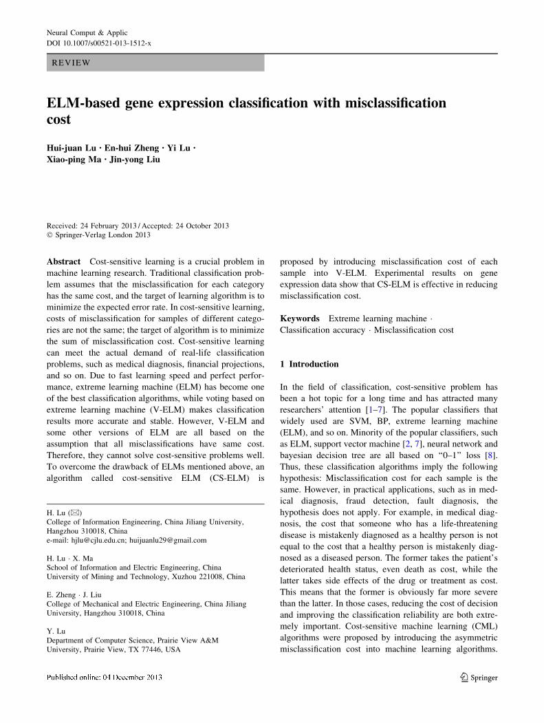
From Figs. 1 and 3, we can see that the average

misclassification costs based on CS-ELM are lower than

those based on V-ELM, and average misclassification cost

of V-ELM and CS-ELM decreases as the size of training

examples increase (Fig. 2).

Neural Comput & Applic

123

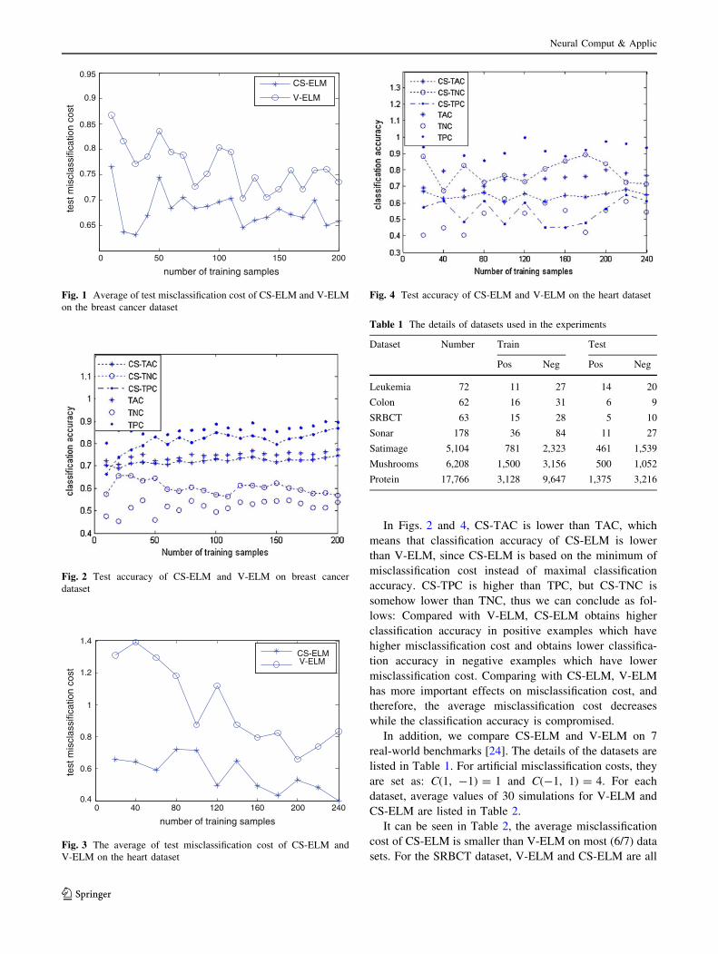
In Figs. 2 and 4, CS-TAC is lower than TAC, which

means that classification accuracy of CS-ELM is lower

than V-ELM, since CS-ELM is based on the minimum of

misclassification cost instead of maximal classification

accuracy. CS-TPC is higher than TPC, but CS-TNC is

somehow lower than TNC, thus we can conclude as fol-

lows: Compared with V-ELM, CS-ELM obtains higher

classification accuracy in positive examples which have

higher misclassification cost and obtains lower classifica-

tion accuracy in negative examples which have lower

misclassification cost. Comparing with CS-ELM, V-ELM

has more important effects on misclassification cost, and

therefore, the average misclassification cost decreases

while the classification accuracy is compromised.

In addition, we compare CS-ELM and V-ELM on 7

real-world benchmarks [24]. The details of the datasets are

listed in Table 1. For artificial misclassification costs, they

are set as: C(1, -1) = 1 and C(-1, 1) = 4. For each

dataset, average values of 30 simulations for V-ELM and

CS-ELM are listed in Table 2.

It can be seen in Table 2, the average misclassification

cost of CS-ELM is smaller than V-ELM on most (6/7) data

sets. For the SRBCT dataset, V-ELM and CS-ELM are all

0 50 100 150 200

0.65

0.7

0.75

0.8

0.85

0.9

0.95

number of training samples

test

mis

clas

sific

atio

n co

st

CS-ELM

V-ELM

Fig. 1 Average of test misclassification cost of CS-ELM and V-ELM

on the breast cancer dataset

Fig. 2 Test accuracy of CS-ELM and V-ELM on breast cancer

dataset

0 40 80 120 160 200 2400.4

0.6

0.8

1

1.2

1.4

number of training samples

test

mis

clas

sific

atio

n co

st

CS-ELMV-ELM

Fig. 3 The average of test misclassification cost of CS-ELM and

V-ELM on the heart dataset

Fig. 4 Test accuracy of CS-ELM and V-ELM on the heart dataset

Table 1 The details of datasets used in the experiments

Dataset Number Train Test

Pos Neg Pos Neg

Leukemia 72 11 27 14 20

Colon 62 16 31 6 9

SRBCT 63 15 28 5 10

Sonar 178 36 84 11 27

Satimage 5,104 781 2,323 461 1,539

Mushrooms 6,208 1,500 3,156 500 1,052

Protein 17,766 3,128 9,647 1,375 3,216

Neural Comput & Applic

123

obtained 100 percent test classification accuracy. In other

words, misclassification cost of V-ELM and CS-ELM are

equal to zero, according to Eq. (19). Therefore, CS-ELM

performs better or equals to V-ELM in all datasets, when

misclassification cost is regarded as final objective.

5 Conclusion

When the misclassification costs of examples are different,

the classification accuracy based standard classification

algorithm cannot directly meet the demands of minimizing

cost in cost-sensitive classification. By coupling probability

estimation and cost minimization, we proposed CS-ELM, a

CS-ELM algorithm. The CS-ELM is proved to be an

effective tool with good performance. When the mis-

classification costs are different in each type of samples,

compared with V-ELM, although the error rate increases

due to the decrease of classification accuracy, average

misclassification cost in CS-ELM remarkably decreases. It

is because in CS-ELM, samples with high misclassification

cost are considered to maintain their classification accu-

racy. As a result, the accuracy of negative sample, which

has low misclassification cost is sacrificed. Since samples

with high misclassification costs have much more impor-

tant effect on the average misclassification cost than those

with low cost, the average misclassification cost decreases

significantly.

Acknowledgments This work was supported by the National Nat-

ural Science Foundation of China (no. 61272315, no. 60842009, and

no. 60905034), Zhejiang Provincial Natural Science Foundation (no.

Y1110342, no. Y1080950) and the Pao Yu-Kong and Pao Zhao-Long

Scholarship for Chinese Students Studying Abroad.

References

1. Han J, Kamber M (2011) Data mining concepts and techniques.

Morgan Kanfnann, San Francisco CA

2. Zheng EH, Li P, Song ZH (2006) SVM-based Cost Sensitive

Mining. Information and Control 3:294299

3. Chow CK (1970) On optimum recognition error and reject

tradeoff. IEEE Trans Inf Theory 1:41–46

4. Foggia P, Sansone C, Tortorella F et al (1999) Mulit-classifica-

tion: reject criteria for the bayesian combiner. Pattern Recognit

32:1435–1447

5. Stefano CD, Sansone C, Vento M (2008) To reject or not to

reject: that is the question-answer in case of neural classifiers.

IEEE Trans SMC 30(1):84–94

6. Landgrebe T, Taxdmj CW, Paclik P et al (2006) The interaction

between classification and reject performance for distance-based

reject-option classifiers. Pattern Recognit Lett 8:908–917

7. Zheng EH et al. (2009) SVM-BASED credit card fraud detection

with reject cost and class-dependent error cost. Proceedings of the

PAKDD’ 09 Workshop: data mining when classes are imbal-

anced and errors have cost. Rangsit Campus: Thammasat Printing

House, 2009: 50–58

8. Zheng EH (2010) Cost sensitive data mining based on support vector

machines: theories and applications. Control and Decision

25(2):191–195

9. Kubat M, Holte R, Matwin S (1997) Learning when negative

examples abound. Machine learning: ECML-97, Lecture Notes in

Artificial Intelligence. Springer. 1224:146–153

10. Chan PK, Stolfo SJ (2001) Toward scalable learning with non-

uniform class and cost distributions: a case study in credit card

fraud detection. Proceedings of the 4th international conference

on knowledge discovery and data mining. 164–168

11. Weiss GM, Provost F (2003) Learning when training data are

costly: the effect of class distribution on tree induction. J Artif

Intell Res 19:315–354

12. Japkowicz N (2000) The class imbalance problem: significance and

strategies. Proceedings of the 2000 international conference on

artificial intelligence: special track on inductive learning, Las Vegas

13. Elkan C (2001) The foundation of cost-sensitive learning. Pro-

ceedings of the 17th international joint conference on artificial

intelligence, Washington. 239–246

14. Zhou ZH, Liu XY (2006) Training cost-sensitive neural networks

with methods addressing the class imbalance problem. IEEE

Trans Knowl Data Eng 18(1):63–77

15. Liu XY, Wu J, Zhou ZH (2009) Exploratory under-sampling for

class-imbalance learning. IEEE Trans Syst Man Cybern-Part B:

Cyber 39(2):539–550

16. Ling C, Li C (1998) Data mining for direct marketing problems

and solutions. Proceedings of the 4th international conference on

knowledge discovery and data mining, New York. 73–79

17. Drummond C, Holte R (1998) Exploiting the cost in sensitivity of

decision tree splitting criteria. Proceedings of the 17th international

conference on machine learning. Stanford University. 73–79

18. Fan W, Stolfo S, Zhang J, Chan P (1999) Adacost: misclassifi-

cation cost-sensitive boosting. Proceedings of the 16th interna-

tional conference on machine learning. Bled, Slovenia. 97–105

19. Freund Y, Schapire RE (1997) A decision-theoretic generaliza-

tion of on-line learning and an application to boosting. J Comput

Syst Sci 55(1):119–139

20. Xiao JH, Pan KQ, Wu JP, Yang SZ (2001) A study on SVM for

fault diagnosis. J Vib Measurement Diagn 21(4):258–262

21. Huang GB, Zhu QY, Siew CK (2006) Extreme learning machine:

theory and applications. Neurocomputing 70:489–501

22. Huang GB, Zhu QY, Siew CK (2004) Extreme learning machine:

a new learning scheme of feedforward neural networks. Pro-

ceedings of international joint conference on neural networks.

25–29

23. Cao JW, Lin ZP, Huang GB, Liu N (2011) Voting based extreme

learning machine. Inf Sci 185(1):66–77

24. Michie D, Spiegelhalter J, Taylor CC Machine learning neural

and statistical classification. http://www.nccup.pt/liacc/ML/

statlog/data.html. 199

Table 2 The experiment results of CS-ELM and V-ELM on different

datasets

Dataset TAC AMC

CS-ELM ELM CS-ELM ELM

Leukemia 0.811 0.875 0.376 0.447

Colon 0.825 0.895 0.279 0.401

SRBCT 1.000 1.000 0.000 0.000

Sonar 0.819 0.856 0.327 0.576

Satimage 0.818 0.863 0.364 0.504

Mushrooms 0.920 0.968 0.087 0.120

Protein 0.729 0.863 0.402 0.524

Neural Comput & Applic

123