DBSDA: Lowering the Bound of Misclassification Rate for

This article has been accepted for inclusion in a future issue of this journal. Content is final as presented, with the exception of pagination.

IEEE TRANSACTIONS ON NEURAL NETWORKS AND LEARNING SYSTEMS 1

DBSDA: Lowering the Bound of MisclassificationRate for Sparse Linear Discriminant Analysis

via Model DebiasingHaoyi Xiong , Member, IEEE, Wei Cheng , Member, IEEE, Jiang Bian, Student Member, IEEE,

Wenqing Hu, Zeyi Sun , and Zhishan Guo, Member, IEEE

Abstract— Linear discriminant analysis (LDA) is a well-knowntechnique for linear classification, feature extraction, and dimen-sion reduction. To improve the accuracy of LDA under thehigh dimension low sample size (HDLSS) settings, shrunkenestimators, such as Graphical Lasso, can be used to strike abalance between biases and variances. Although the estimatorwith induced sparsity obtains a faster convergence rate, however,the introduced bias may also degrade the performance. In thispaper, we theoretically analyze how the sparsity and the con-vergence rate of the precision matrix (also known as inversecovariance matrix) estimator would affect the classification accu-racy by proposing an analytic model on the upper bound of anLDA misclassification rate. Guided by the model, we propose anovel classifier, DBSDA, which improves classification accuracythrough debiasing. Theoretical analysis shows that DBSDApossesses a reduced upper bound of misclassification rate andbetter asymptotic properties than sparse LDA (SDA). We conductexperiments on both synthetic datasets and real applicationdatasets to confirm the correctness of our theoretical analysisand demonstrate the superiority of DBSDA over LDA, SDA,and other downstream competitors under HDLSS settings.

Index Terms— Classification, debiasing, linear discriminantanalysis, sparsity.

I. INTRODUCTION

L INEAR discriminant analysis (LDA) [1] is a well-knowntechnique for feature extraction and dimension reduc-

tion [2]. It has been widely used in many applications, such asface recognition [3], image retrieval, and so on. An intrinsiclimitation of classical LDA is that its objective function relieson the well-estimated and nonsingular covariance matrices.For many applications, such as the microarray data analysis, all

Manuscript received August 2, 2017; revised March 1, 2018 andJune 1, 2018; accepted June 1, 2018. (Corresponding author: Haoyi Xiong.)

H. Xiong is with the Big Data Laboratory, Baidu Research, Beijing100193, China, and also with the National Engineering Laboratory ofDeep Learning Technology and Application, Beijing 100193, China (e-mail:[email protected]).

W. Cheng is with the NEC Labs of America, Princeton, NJ 08540 USA.J. Bian is with the Big Data Laboratory, Baidu Research, Beijing 100193,

China, and also with the Department of Computer Science, Missouri Univer-sity of Science and Technology, Rolla, MO 65409 USA.

W. Hu and Z. Sun are with the Department of Mathematics and Statistics,Missouri University of Science and Technology, Rolla, MO 65409 USA.

Z. Guo is with the Department of Computer Science, Missouri Universityof Science and Technology, Rolla, MO 65409 USA.

Color versions of one or more of the figures in this paper are availableonline at http://ieeexplore.ieee.org.

Digital Object Identifier 10.1109/TNNLS.2018.2846783

scatter matrices can be singular or ill-posed since the data areoften with high dimension but low sample size (HDLSS) [4].

The classical LDA classifier relies on two keyparameters–the mean vector of each type and the precisionmatrix. Under the HDLSS settings, the sample precisionmatrix (also known as the inverse of sample covariance matrix)used in LDA is usually ill-estimated and quite different fromthe inverse of population/true covariance matrix [5]. Forexample, the largest eigenvalue of the sample covariancematrix is not a consistent estimate of the largest eigenvalue ofthe population covariance matrix, and the eigenvectors of thesample covariance matrix can be nearly orthogonal to the truthwhen the number of dimensions is greater than the number ofsamples [6], [7]. Such inconsistency between the true and theestimated precision matrices degrades the accuracy of LDAclassifiers under the HDLSS settings [8], [9].

A plethora of excellent work has been conducted toaddress such HDLSS data classification problem. For exam-ple, Krzanowski et al. [10] suggested to use pseudoinverseto approximate the inverse covariance matrix, when thesample covariance matrix is singular. However, the preci-sion of pseudoinverse LDA is usually low and not wellguaranteed [11]. Other techniques include the two-stagealgorithm principle component analysis + LDA [11], [12],LDA based on Kernels [13]–[16] and/or other nonpara-metric statistics [17]–[20]. To overcome the singularityof the sample covariance matrices, instead of estimatingthe inverse covariance matrix and mean vectors separately,Clemmensen et al. [21], Cai and Liu [22], and Mai et al. [23]proposed to estimate the projection vector for discriminationdirectly. More popularly, regularized LDA approaches [3],[10], [24] are proposed to solve the problem. These meth-ods can improve the performance of LDA either empiri-cally or theoretically, while few of them can directly addressthe ill-estimated inverse covariance matrix estimation issue.

One representative regularized LDA approach is to replacethe precision matrix used in LDA with a shrunken estima-tor [3], [10], [24], such as Graphical Lasso [25], so as toachieve a “superior prediction.” Intuitively, through replacingthe precision matrix used in LDA with a sparse regularizedestimation, the ill-posed problem caused by HDLSS settingscan be well addressed. The sparse estimators usually convergeto the inverse of true/population covariance matrix faster than

2162-237X © 2018 IEEE. Personal use is permitted, but republication/redistribution requires IEEE permission.See http://www.ieee.org/publications_standards/publications/rights/index.html for more information.

https://orcid.org/0000-0002-5451-3253

https://orcid.org/0000-0001-5456-626X

https://orcid.org/0000-0003-0704-2708


2 IEEE TRANSACTIONS ON NEURAL NETWORKS AND LEARNING SYSTEMS

the sample estimators [5]. With the asymptotic properties,the sparse LDA (SDA) should be close to the optimal LDA.However, the way that the sparsity and the convergence rate ofthe precision matrix estimator would affect the classificationaccuracy is not well studied in the literature.

Furthermore, with induced sparsity, the inverse covarianceestimator becomes biased [26]. The performance of SDAis frequently bottlenecked due to the bias of the sparseestimators. Recently, researchers tried to debias the Lassoestimator [26]–[28], through adjusting the �1-penalty for theregularized estimation, so as to achieve a better regressionperformance. Inspired by this line of research, we proposeto improve SDA through debiasing (i.e., desparsifing) inthis paper.

Our Contributions: With respect to the aforementionedissues, in this paper, we made following contributions.

1) We propose a novel analytic model for the LDA misclas-sification rate, based on the convergence rate of inverse)covariance matrix estimator and the sparsity/density ofthe estimates. This model can derive the upper boundsof LDA misclassification rate on both the Gaussian andnon-Gaussian datasets.

2) Guided by the proposed analytic model, we first analyzethe most commonly seen SDA via Graphical Lasso [24],and study the upper bounds of the SDA misclassificationrate. Inspired by debiased Lasso [28], we then develop anovel classifier DBSDA—debiased sparse discriminantanalysis. DBSDA leverages yet another debiased esti-mator for a linear classification problem, to reduce theupper bounds of misclassification rate, through balanc-ing the biases and variances in a regularized model.

3) Our theoretical analysis based on the proposed analyticmodel shows, in terms of asymptotic properties of pro-jection vector (also known as the vector β), DBSDAconverges faster than SDA; in terms of misclassifi-cation rate, DBSDA enjoys a reduced upper boundof misclassification rate than SDA. We also conductextensive experiments to demonstrate the advantage ofthe proposed algorithms comparing to other competitors.The results validate the correctness of our theoreticalanalysis.

The paper is organized as follows. In Section II, we reviewthe LDA models and summarize the existing LDA misclas-sification rate analysis model. In Section III, we propose ananalytic model characterizing the error bound of misclassi-fication rate based on the sparsity and convergence rate ofan inverse covariance matrix estimator. In Section IV, guidedby the proposed analytic model, we introduce a baselinealgorithm SDA, then propose our algorithm, DBSDA, andfurther compare their performances. In Section V, we vali-date the proposed algorithms, synthesized datasets, benchmarkdatasets, and real-world applications. Finally, we review therelated work, discuss the limitation, and conclude the paper inSections VI and VII, respectively.

II. PRELIMINARIES

In this section, we first briefly introduce the binary classifierusing traditional LDA. Then, we present the state-of-the-art

TABLE I

SUMMARY OF NOTATIONS

analytic models on the LDA misclassification rate whichassume that the data for classification follow certain Gaussiandistributions. The main notations are listed in Table I.

A. LDA for Binary Classification

To use Fisher’s LDA (FDA), given the independent identi-cally distributed (i.i.d.) labeled data pairs (x1, l1) . . . (xm, lm),we first estimate the sample covariance matrix � using thepooled sample covariance matrix estimator with respect to thetwo classes [1], then estimate the sample precision matrix as� = �−1. Furthernore, μ+ and μ− are estimated as the meanvectors of the positive samples and the negative samples inthe m training samples, respectively.

Given all estimated parameters � (and � = �−1),μ+ and μ−, the FDA model classifies a new data vector xas the result of

f (x) = argmax�∈{−,+}

δ(x, �, μ�, π�)

where

δ(x, �, μ�, π�) = x T �μ� − 1

2μT

� �μ� + log π� (1)


XIONG et al.: DBSDA: LOWERING THE BOUND OF MISCLASSIFICATION RATE FOR SDA VIA MODEL DEBIASING 3

where π+ and π− refer to the (foreknown) frequencies ofpositive samples and negative samples in the whole population,respectively.

B. LDA Misclassification Rate for Gaussian Data WithUncertain Covariance Estimates

In this section, we summarize the studies [8], [9], [29], [30]in theoretical misclassification rate of LDA classifiers forclassifying multivariate Gaussian data.

We first assume that the data for binary classificationfollow two (unknown) Gaussian distributions with the samecovariance matrix �∗ (i.e., the inverse covariance matrix�∗ = �∗−1) but two different means μ∗+ and μ∗−,i.e., N (μ∗+,�∗) for positive samples and N (μ∗−,�∗) fornegative samples, respectively. Given the LDA classifierf (x) based on the sample estimated mean vectors μ+,μ−, and a specific covariance matrix � (and � = �−1),Zollanvari et al. [8] and Zollanvari and Dougherty [9]modeled the expected misclassification rate of an LDA(i.e., probability of � �= f (x)) on the data of N (μ∗+,�∗),N (μ∗−,�∗) as a function ε(μ+, μ−, �, μ∗+, μ∗−, �∗),that is,

ε(μ+, μ−, �, μ∗+, μ∗−,�∗

)

= π+ ·⎛

⎜⎝−

(μ∗+ − (μ++μ−)

2

)T�(μ+ − μ−)

√(μ+ − μ−)T ��∗�(μ+ − μ−)

⎞

⎟⎠

+π− ·⎛

⎜⎝

(μ∗− − (μ++μ−)

2

)T�(μ+ − μ−)

√(μ+ − μ−)T ��∗�(μ+ − μ−)

⎞

⎟⎠

= π+ ·(

(2(μ+ − μ∗+)− (μ+ − μ−))T �(μ+ − μ−)

2√

(μ+ − μ−)T ��∗�(μ+ − μ−)

)

+π− ·(

(2(μ∗− − μ−)− (μ+ − μ−))T �(μ+ − μ−)

2√

(μ+ − μ−)T ��∗�(μ+ − μ−)

)

(2)

where � = �−1 and (·) refers to the CDF functionof a standard normal distribution. It is obvious that theexpected misclassification rate is sensitive with the parame-ters μ∗+, μ∗−,�∗, μ+, μ−, and �, while the true parametersμ∗+, μ∗−, and �∗ are usually unknown.

Assumption 1: Given m samples x1, x2, . . . , xm drawn fromN (μ∗+,�∗) and N (μ∗−,�∗) with constant priors, μ+ andμ− are estimated using sample estimators. According to [31],the sample mean μ+, μ−, and μ converge to the popula-tion mean μ∗+, μ∗−, and μ∗ at the �2-norm convergence rateO(p/m)1/2 in high probability.

Assumption 2: We assume that for each sample |xi |2 ≤ L.Thus, there has |μ+ − μ−|2 ≤ 2L. For sample covariancematrix � = m−1 ∑m

i=1 xi x Ti , there has ��2 = λmax(�) ≤

trace(�) ≤ L2, as � is a positive semidefinite matrix with alleigenvalues nonnegative.

Assumption 3: As was assumed in [32] and [33],we assume that there exists a positive constant K that

can bound the eigenvalues of �∗ as 1/K ≤ λmin(�∗) ≤

λmax(�∗) ≤ K . Since �∗ = �∗−1, then there also exists

1/K ≤ λmin(�∗) ≤ λmax(�

∗) ≤ K. In this way, there exist��∗�2 ≤ K and ��∗�2 ≤ K.

Theorem 1: We first denote �μ as �μ = μ+ − μ−.Then, based on [8] and [9], the upper bound of the expectedmisclassification rate of f (x) can be reduced to

P∼N [� · f (x) < 0] ≤

⎛

⎝C√

p/m · |��μ|2 − �Tμ��μ

2√

�Tμ��∗��μ

⎞

⎠

(3)

where C refers to a positive constant.Intuitively, when the sample estimation of a covariance

matrix � (also �) is close to the population ones �∗ (and �∗),the expected error rate can be minimized.

III. MAIN THEORY: UPPER BOUNDS OF

LDA MISCLASSIFICATION RATES

In this section, we analyze the performance of a classicalLDA classifier. We derive the upper bounds of the LDA mis-classification rate on both the Gaussian and non-Gaussian data.Our result shows, for both the Gaussian and non-Gaussiandatasets, the upper bounds of LDA misclassification rates aresensitive to the sparsity of inverse covariance matrix estimatorand the convergence rate of the estimator.

A. LDA Misclassification Rate for Gaussian Data

Let denote �μ = |μ+ − μ−|2/2 referring the gap betweenmeans, in the rest of this paper.

Theorem 2: Suppose the data for the binary classifica-tion (training and testing) follows the Gaussian distributionsN (μ∗+,�∗) and N (μ∗−,�∗) (with �∗ = �∗−1). Given aninverse covariance matrix estimator � and mean estimatorsμ+ and μ− over m samples drawn from the distribution withconstant priors, the misclassification rate of f (x) will be upperbounded by

P∼N [� · f (x) < 0] ≤

(C

2

√K · p

m− |�μ|2

2√KL2

��−12

).

(4)

Theorem 1 suggests that the performance of LDA can beimproved with lower misclassification upper bound, whenusing a sparse inverse covariance matrix estimator with fasterconvergence rate in spectral norm.

Proof: To prove Theorem 1, given the symmetric positivedefinite matrices �∗ and �∗ = �∗−1, there must exist theCholesky decomposition matrix M having �∗ = MT M and�∗−1 = �∗ = M−1(M−1)T

P[� · f∼N (x) ≤ 0] ≤

(C√

p/m · |��μ|2 − �Tμ��μ

2|M��μ|2

)

.

Since (·) is monotonically increasing, we have

P[� · f∼N (x) ≤ 0] ≤

(C

2

√p

m· �M−1�2 −

�Tμ��μ

2|M��μ|2

)

.



Since there exists (1) �M−1�2 = (λmax((M−1)T M−1))1/2 =(λmax(�

∗))1/2 ≤ (K)1/2. (2) �Tμ��μ ≥ λmin(�)|�μ|22 =

1/λmax(�) · |�μ|22 ≥ (1/L2)|�μ|22, and (3) �M�2 =(λmax(MT M))1/2 = (λmax(�

∗))1/2 ≤ (K)1/2, then we have

P[� · f∼N (x) ≤ 0] ≤ (

C2

√K · p

m − |�μ|22√KL2 ��−1

2

).

�

B. LDA Misclassification Rate for Non-Gaussian Data

In this section, we generalize the LDA misclassification ratefrom Gaussian data to non-Gaussian data.

Theorem 3: Suppose the labeled data pairs (x, �) followsa joint probability distribution with density function P(x, �).The population covariance matrix �∗ is defined as

�∗ = Ex

i.i.d.∼ P(X)[(X− μ)(X− μ)T] (5)

where μ is the sample mean estimated from the trainingsamples drawn i.i.d. from an unknown distribution with densityfunction P(x) = ∑

�∈{−1,+1} P(x, �). Based on our assump-tion on mean vectors, the Gaussian distribution N (μ,�∗) isthe nearest Gaussian distribution to the data, with minimizedKullback–Leibler divergence [34]. Then, there exists an upperbound of f (x)’s misclassification rate on such data

P[� · f (x) < 0]≤ P∼N [� · f (x) < 0] +

∑

�∈{−1,+1}π�

√DKL (P��N (μ�,�∗))

2

(6)

where P� refers to the distribution of data x with a specificlabel � ∈ {+1,−1} and the probability density function isP(x |�) = (P(x, �)/π�), and DKL(P��N (μ�,�

∗)) refers tothe Kullback–Leibler divergence between the distribution ofthe data and Gaussian distribution N (μ�,�

∗).Proof: Given an LDA classifier f (x) : X → {+1,−1},

we define the misclassification function 1[� �= f (x)] = 1when � �= f (x) and 1[� = f (x)] = 0 when � = f (x). Then,the misclassification rate of f (x), for any data distribution withdensity functions P(x, �) and � ∈ {+1,−1}, can be written as

P[l · f (x) < 0] =∑

�∈{+1,−1}

∫

x1[� �= f (x)] · P(x, �)dx .

Consider the density functions P∼N (x |�) for Gaussian distri-bution N (μ�,�

∗) and � ∈ {+1,−1}P[l · f (x) < 0]=

∑

�∈{+1,−1}

∫

x1[� �= f (x)] · π� · P∼N (x |�)dx

+∑

�∈{+1,−1}

∫

x1[� �= f (x)] · π� · (P(x |�)− P∼N (x |�))dx .

Consider the misclassification rate on Gaussian distributionP∼N [� · f (x) < 0]. Thus

P[l · f (x) < 0] ≤ P∼N [� · f (x) < 0]+

∑

�∈{+1,−1}π�

∫

x|P(x |�)−P∼N (x |�)|dx .

Consider Pinsker’s inequality

P[l · f (x) < 0]≤ P∼N [� · f (x) < 0] +

∑

�∈{−1,+1}π�

√DKL (P��N(�∗,μ�))

2

where DKL (P��N(�∗,μ�)) refers to the Kullback–Leibler diver-gence (KLD) between the Gaussian distribution N (μ�,�

∗)to the arbitrary distribution P� with the density functionP(x |�) = (P(x, �)/π�). While the KLD of a given datasetto its nearest Gaussian distributions are frequently fixed,the misclassification rate of f (x) on arbitrary data distributionis sensitive with the Gaussian bound P∼N [� · f (x) < 0]. �

Remark 1: Theorem 2 suggests that we can consider anydistribution as the combination of its nearest Gaussian dis-tribution [i.e., N (μ,�∗)] and other non-Gaussian compo-nents [35]. Given an LDA classifier f (x), the misclassificationrate is affected by two factors: 1) the misclassification rateof f (x) on the nearest Gaussian distribution of the data,i.e., P∼N [� · f (x) < 0] and 2) the divergence betweenthe data distribution and the Gaussian distribution. Since thedivergence of the given data to its nearest Gaussian distributionDKL(P��N (μ�,�

∗)) is fixed for a non-Gaussian dataset,we only need to consider the first term of the right-hand sidein the inequality. Considering both the theorems, we can thusfurther conclude that for any datasets, the performance of f (x)is sensitive to the convergence rate �� − �∗�2. Such factoris sometimes known or bounded when an estimator is given,thus are the focuses of this paper.

IV. PROPOSED ALGORITHM

In this section, we first introduce a baseline algorithmthat lowers the aforementioned error bound using the sparsebut biased precision matrix estimator with fast convergencerate. Then, we propose our algorithm DBSDA that furtherimproves the baseline algorithms through the model debiasing.Finally, we discuss the theoretical advantages of the proposedalgorithm.

A. Sparse Discriminant Analysis via Graphical Lasso

This baseline algorithm, referred to by SDA via GraphicalLasso, was derived from the Scout family of LDA introducedin [24]. Compared to the classical Fisher’s LDA presentedin Section II-A, this baseline algorithm leverages GraphicalLasso [24] estimator to replace the precision matrix estimatedusing sample covariance matrix. The proposed algorithm isimplemented using the discriminant function defined in (1), as

f (x) = argmax�∈{−,+}

δ(x, �, μ�, π�) (7)

where � refers to the Graphical Lasso estimator based on thesample covariance matrix �

� = argmin�>0

⎛

⎝tr(��)− log det(�)+ λ∑

j �=k

|� j k|⎞

⎠. (8)



According to Theorem 1 and the convergence rate of GraphicalLasso [36], the misclassification rate of f (x) is addressedin Theorem 3.

Theorem 4: Suppose the sample covariance matrix isestimated using m samples drawn i.i.d. from a Gaussiandistribution N (μ,�∗), the upper bound of the misclassifica-tion rate of f (x) on Gaussian distributions—N (μ+,�∗) andN (μ−,�∗)—should be

P∼N [� · f (x) < 0]=

(

O(

( p

m

) 12 −

(m

12

m12 + ((p + d) log p)

12

)))

(9)

with high probability, where the rate ((p + d) log p/m)1/2 isderived from the Frobenius-norm convergence rate of Graph-ical Lasso [36], and d = max1≤i≤p|{ j : �∗−1

i, j �= 0}| refersto the maximal degree of the graph (i.e., population inversecovariance matrix).

Proof: According to Zollanvari’s model, the misclassifi-cation rate of f (x) on the Gaussian data should be

P∼N [� · f (x) < 0] = ε(μ+, μ−, �, μ∗+, μ∗−,�∗

)(10)

where �−1 = � is the Graphical Lasso estimator.According to [36], while the spectral-norm convergence rate

is not yet known, the Frobenius-norm convergence rate ofGraphical Lasso is known as

��2 ≤ ��∗�2 + ��−�∗�2 ≤√K + ��−�∗�F

= Op

(√m +√

(p + d) log p√m

)

(11)

where d = max1≤i≤p |{ j : �∗ �= 0}| refers to the maximaldegree of the true graph �∗ = �∗−1. Then, according to thedefinition of O(·), we can conclude

P∼N [� · f (x) < 0]=

(

O(( p

m

) 12 − m

12

m12 + ((p + d) log p)

12

))

. (12)

�

B. DBSDA: Debiased Sparse Discriminant Analysis

Intuitively, a sparse estimator, such as SDA aforementioned,can be further improved through debiasing. For example,Lasso can be improved, with even faster convergence rate(lower error bound), by debiased Lasso [28].

In this section, we introduce our proposed algorithmDBSDA(via Graphical Lasso). We first present the linear clas-sifier form of the SDA. Then, we propose a debiased estimatorof the linear projection vector (i.e., β), which is derived fromthe well-known debiased Lasso. Later, we address the overallalgorithm design.

The SDA algorithm introduced in (7) can be rewritten in alinear classifier form as

f (x) = sign(δ(x, �, μ+, π+)− δ(x, �, μ−, π−))

= sign(xT βG + cg) (13)

where sign(·) function returns +1 if the input is nonnega-tive, and −1 when the input is negative. The vector βG =�(μ+ − μ−) and the scalar cg = −(1/2) · (μ+ + μ−)T βG +log(π+/π−). Obviously, βG is the vector of projection coef-ficients for linear classification.

Inspired by the debiased Lasso [26]–[28], we propose toimprove the performance of SDA through debiasing βG .Given m labeled training data (x1, �1), (x2, �2), . . . (xm .�m)with balanced labels, the Graphical Lasso estimator � on thedata and the SDA model (i.e., βG and cg), we propose a noveldebiased estimator of β D that takes the form as

β D ← βG + 1

m· �(X− U)T (L− XT βG − Cg) (14)

where we denote X as an m × p matrix, where 1 ≤ i ≤ mand the i th column is xi ; L as a 1 × m matrix (i.e., vector)whose i th row is �i ; U is an m × p matrix with each columnas (μ+ + μ−/2); and Cg is a p-dimensional vector with eachrow as cg . Note that the debiased estimator addressed in (14)is quite different from debiased Lasso [28], with respect to thestructure of LDA as a classifier. We analyze the performanceof debiased estimator in Section IV-C.

Given the debiased estimator β D, our proposed algorithmDBSDA is designed as

f D(x) = sign

((x T − μ+ + μ−

2

)T

β D + log(π+/π−)

)

.

(15)

In Section IV-C, we present the analytical results of DBSDA.

C. Theoretical Properties of DBSDAIn this section, we first present Theorem 4 that provides a

upper bound of the misclassification rate of DBSDA. Then,we present Theorem 5 addressing asymptotic properties of β D .Finally, we remark the theoretical performance comparisonbetween DBSDA and SDA.

1) DBSDA—Misclassification Rate Analysis: Further,we aim at analyzing the effect of convergence rates to theupper bound of DBSDA misclassification rate. Then, we havethe following theorem.

Theorem 5: Under the same conditions, the upper boundof f D(x) misclassification rate on Gaussian distributionsN (μ∗+,�∗) and N (μ∗−,�∗) (with equal priors) should be

P∼N [� · f D(x) < 0]=

(

O(

( p

m

) 12 − m

12

m12 + (p log p)

12

))

(16)

with high probability.Lemma 1: Consider the definition of the debiased LDA

estimator β D introduced in (14), we have

β D = βG + 1

m· �XT L − 1

m· �UT L

− 1

m· �(X− U)T (X− U)βG . (17)

As was defined βG = �(μ+ − μ−) = (1/m) · �XT L. Withthe assumption of equal priors (π+ = π− = 0.5), thus L is



a label vector that half of its elements are +1 while the rest areall −1. As U is matrix where each column is a constant vector(μ+ + μ−)/2, thus (1/m) · �UT L = 0. As each column of Xrefers to a sample drawn from the original data distribution,thus (1/m)(X − U)T (X − U) = � is the sample covariancematrix estimator. With all above in mind, we have

β D = βG + (I− ��)βG = (2�− ��)�μ (18)

where I refers to a p× p identity matrix. Note that (I−��)βG

can be considered the desparsification term that debiases βG

through adjusting the Karush–Kuhn–Tucker (K.K.T) conditiongiven the Graphical Lasso estimator.

Proof: As was mentioned in Lemma1, DBSDA indeedcan be considered as an LDA classifier that leverages �D asits precision matrix estimator and �D = (2 · � − ��).Considering the known Frobenius-norm convergence rate

��D�2 ≤ ��∗�2 + ��D −�∗�2 ≤√K+ ��−�∗�F

= Op√

p log p/m. (19)

According to the definition of O(·), we can obtain the result

P∼N [� · f D(x) < 0]=

(

O(

( p

m

) 12 − m

12

m12 + (p log p)

12

))

(20)

with high probability. �2) DBSDA—Asymptotic Analysis: In order to analyze the

performance of DBSDA, we first define the linear projectionvector of the optimal LDA as β∗ = �∗−1(μ∗+ − μ∗−), thenwe intend to understand how close βG and β D approximateto the optimal estimation β∗. Here, we continue assuming thepopulation mean vectors μ∗, μ∗+, and μ∗− are estimated assample mean vectors μ, μ+, and μ−, and have the followingtheorem:

Theorem 6: Given the m samples for training (x1, �1), . . . ,(xm, �m) drawn i.i.d. from N (μ∗+,�∗) and N (μ∗−,�∗) withthe equal priors, the �∞-vector-norm convergence rate ofβ D and βG approximating to the optimal estimation β∗ are

|β D − β∗|2 = Op(√

p log p/m)

|βG − β∗|2 = Op(√

(p + d) log p/m) (21)

under the assumption that |μ∗+ − μ∗−|2 is estimated as|μ+ − μ−|2 and |μ∗+ − μ∗−|2 is assumed a constant.

Proof: Here, we first prove the upper bound of|βG − β∗|∞. As was defined βG = �(μ+ − μ−), then wehave

|βG − β∗|2 =∣∣�(μ+ − μ−)−�∗

(μ∗+ − μ∗−

)∣∣2

≤ ∣∣(�−�∗)�μ|2 + |�∗

(μ∗+ − μ+

)∣∣2

+ ∣∣�∗

(μ∗− − μ−

)∣∣2

≤ ��−�∗�2 · |�μ|2+��∗�2 ·

(∣∣μ∗+ − μ+∣∣2 +

∣∣μ∗− − μ−∣∣2

). (22)

Since 1) both μ+ and μ− converge at the rate Op(√

p/m) in�2-norm; 2) the spectral-norm convergence rate of � [32] is�� − �∗�2 ≤ �� − �∗�F = Op(((p + d) · log p/m)1/2);

and 3) �μ ≤ 2L is bounded by a constant, we thus canconclude that, with high probability

|βG − β∗|2 = Op(√

(p + d) · log p/m). (23)

�Proof: Given Lemma 1, we prove the upper bound of

|β D − β∗|2 as

|β D − β∗|2 =∣∣(2�− ��)(μ+ − μ−)−�∗

(μ∗+ − μ∗−

)∣∣2

≤ |(2�− ��−�∗)(μ+ − μ−)|2+ ∣

∣�∗(μ∗+ − μ+

)∣∣2 +

∣∣�∗

(μ∗− − μ−

)∣∣2

≤ �2�− ��−�∗�2 · |μ+ − μ−|2+��∗�2 ·

(∣∣μ+ − μ∗+∣∣2 +

∣∣μ− − μ∗−

∣∣2

). (24)

According to [33], the spectral-norm convergence rate of thedesparisified estimator �D = (2 · � − ��) under mildconditions should be ��D − �∗�2 ≤ √p · ��D − �∗�∞ =Op(p · log p/m)1/2. In this way, considering Assumption 1,we conclude the convergence rate as

|β D − β∗|2 = Op(√

p log p/m). (25)

�Note that, to highlight the effect of precision matrix to theaccuracy of classification, throughout the paper, we make noassumptions on the mean vectors. We consider the sampleestimation μ, μ+, and μ− as the mean vectors μ∗, μ∗+, andμ∗− in the Gaussian distribution. It is quite often in multivariatestatistics to follow such settings [31].

Remark 2: Compared to SDA’s βG , our method DBSDArecovers the linear projection vector β D with a faster con-vergence rate, i.e., (log p/m)1/2 < ((p + d) · log p/m)1/2

in a mild condition. Thus, we can conclude that DBSDAoutperforms SDA with reduced upper bounds of �∞ vectornorm estimation errors. We name β D as the debiased estimatorof βG due to following reasons: with assumptions addressedin Theorem 4, we can rewrite βG = �(μ+ − μ−) andβ D = (2 · �− ��)(μ+ − μ−), while (2 · �− ��) is thedebiased estimator of �, according to [33].

Remark 3: In terms of misclassification rate comparison,Op((p log p/m)1/2) < Op(((p + d) log p/m)1/2) while theB = �(I − ��)��2 is not fully known. However, �� shouldbe very close to the identity matrix I , considering the K.K.Tcondition in (8). In this way, f D(x) can outperform f G (x)with lower misclassification rate.

V. EXPERIMENTS

In this section, we first validate different properties ofDBSDA on the synthesized data, from which we can gaininsight into the superiority of DBSDA. Then, we experi-mentally evaluate the performance of DBSDA on benchmarkdatasets, in terms of the accuracy for binary classification.Finally, we demonstrate the performance of DBSDA onreal-world HDLSS dataset for the application of diseases earlydetection.



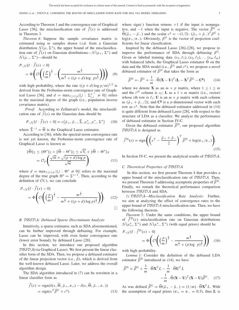
Fig. 1. Classification accuracy of DBSDA versus SDA on pseudorandomsynthesized data. (a) DBSDA versus SDA. (b) λ Tunning.

A. Synthesized Data Evaluation

To validate our algorithms, we evaluate our algorithms ona synthesized dataset, which are obtained through a pseudo-random simulation. The synthetic data are generated by twopredefined Gaussian distributions N (μ∗+,�∗) and N (μ∗−,�∗)with equal priors. The settings of μ∗+, μ∗−, and �∗ are asfollows: �∗ is a p× p symmetric and positive definite matrix,where each element �∗i, j = 0.8|i− j |, 1 ≤ i ≤ p and1 ≤ j ≤ p. μ∗+ and μ∗− are both p-dimensional vectors,where μ∗+ = 1, 1, . . . , 1, 0, 0, . . . , 0�T (the first 10 elementsare all 1’s, while the rest p−10 elements are 0’s) and μ∗− = 0.(Settings of the two Gaussian distributions first appear in [37].)In our experiment, we set p = 200. To simulate the HDLSSsettings, we train SDA and DBSDA, with 20–200 samplesrandomly drawn from the distributions with equal priors, andtest the two algorithms using 500 samples. For each setting,we repeat the experiments for 100 times and take the averagedresults, under the aforementioned cross-validation procedure.

In this experiment, we compare DBSDA, SDA, and LDA(with pseudoinverse). The results of LDA are not includedhere, as it performs extremely worse than both SDA andDBSDA under the HDLSS settings. Fig. 1(a) presents thecomparison between DBSDA and SDA, in terms of accuracy,where each algorithm is fine-tuned with the best parame-ter λ. A detailed example of parameter tuning is reportedin Fig. 1(b), where we run both the algorithms, with training

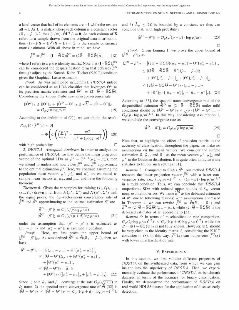
Fig. 2. Classification accuracy of DBSDA versus SDA on unbalanceddatasets (m = 160).

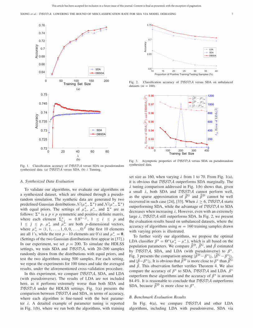
Fig. 3. Asymptotic properties of DBSDA versus SDA on pseudorandomsynthesized data.

set size as 160, when varying λ from 1 to 70. From Fig. 1(a),it is obvious that DBSDA outperforms SDA marginally. Theλ tuning comparison addressed in Fig. 1(b) shows that, givena small λ, both SDA and DBSDA cannot perform well,as the sparse approximation of βG and β D cannot be wellrecovered in such case [24], [33]. When λ ≥ 6, DBSDA startsoutperforming SDA, while the advantage of DBSDA to SDAdecreases when increasing λ. However, even with an extremelylarge λ, DBSDA still outperforms SDA. In Fig. 2, we presentthe evaluation results based on unbalanced datasets, where theaccuracy of algorithms using m = 160 training samples drawnwith varying priors is illustrated.

To further verify our algorithms, we propose the optimalLDA classifier β∗ = �∗(μ∗+ −μ∗−), which is all based on thepopulation parameters. We compare β D , βG , and β estimatedby DBSDA, SDA, and LDA (with pseudoinverse) to β∗.Fig. 3 presents the comparison among |β D−β∗|2, |βG−β∗|2,and |β−β∗|2. It is obvious that β D is more close to β∗ than βG

and β. This observation further verifies Theorem 4. We alsocompare the accuracy of β∗ to SDA, DBSDA and LDA. β∗outperform these algorithms and the accuracy of β∗ is around84.4%. It is reasonable to conclude that DBSDA outperformsSDA, because β D is more close to β∗.

B. Benchmark Evaluation Results

In Fig. 4(a), we compare DBSDA and other LDAalgorithms, including LDA with pseudoinverse, SDA via



TABLE II

EARLY DETECTION OF DISEASES ACCURACY COMPARISON BETWEEN DBSDA AND BASELINES

Fig. 4. Performance comparison on benchmark datasets (p = 300 andp � m). (a) DBSDA versus LDA baselines. (b) DBSDA versusdownstream classifiers.

Graphical Lasso, and Ye-LDA derived from [38], on the Webdatasets [39]. To simulate the HDLSS settings ( p � m),we vary the training sample sizes from 30 to 120 whileusing 400 samples for testing. The numbers of dimensionsp is 300. For each algorithm, the reported result is averagedover 100 randomly selected subsets of the training/testing datawith equal priors. SDA and DBSDA are fine-tuned with thebest λ. The experimental settings show that DBSDA con-sistently outperforms other competitors in different settings.

The nonmonotonic trend of LDA with the increasing trainingset size is partially due to the poor/uncontrollable performanceof pseudoinverse used in LDA. Note that the whole Webdataset consists of three subsets (Web-1, Web-2, and Web-3).Due to space limitation, we only report the results on Web-1in Fig. 4(a). Similar results can be observed on Web-2and Web-3.

In addition to LDA classifiers, we also compared DBSDAwith other downstream algorithms including Decision Tree,Random Forest, Linear Support Vector Machine (SVM), andKernel SVM with Gaussian Kernel. The comparison resultsare listed in Fig. 4(b). All algorithms are fine-tuned with thebest parameters under our experiment settings (under crossvalidation).

C. Early Detection of Diseases on EHR Datasets

To demonstrate the effectiveness of DBSDA in handlingthe real problems, we evaluate DBSDA on the real-worldElectronic Health Records (EHRs) data for early detectionof diseases [40]. In this application, each patient’s EHR dataare represented by a p = 295 dimensional vector, referringto the outpatient record on the physical disorders diagnosed.Patients are labeled with either “positive” or “negative,” indi-cating whether he/she was diagnosed with depression andanxiety disorders. Through supervised learning on the datasets,the trained binary classifier is expected to predict whethera (new) patient is at risk or would develop to the depressionand anxiety disorders from their historical outpatient records(physical disorder records) [41].

We evaluate DBSDA and other competitors, includinglinear SVM, nonlinear SVM with Gaussian kernel, decisiontree, AdaBoost, random forest, and other LDA baselines, withvarying training dataset size m from 100 to 700. Table IIpresents the comparison results. To simplify the comparison,we only present the results of the algorithm with fine-tunedparameter, which is selected through 10-fold cross validation.It is obvious that DBSDA and SDA outperform other baselinealgorithms significantly, while DBSDA performs better thanSDA. The advantage of DBSDA over other algorithms, suchas SVM, is extremely obvious when the size of a trainingdataset m is small. With the increasing sample size, though



TABLE III

EARLY DETECTION OF DISEASES F1-SCORE COMPARISON BETWEEN DBSDA AND OTHER BASELINES

the margins of DBSDA over the rest of algorithms decrease,DBSDA still outperforms other algorithms. We also measuredthe F1-score of all algorithms, DBSDA still outperforms othercompetitors in most cases, which is shown in Table III.

VI. RELATED WORK AND DISCUSSION

In this section, we review several most relevant studiesof our research. To address the HDLSS issues for LDA,a line of research [21], [22], [42], [43] proposed to directlyestimate a sparse projection vector without estimating theinverse covariance matrix (sample covariance matrix is notinvertible) and mean vectors separately. On the otherhand, Peck and Ness [3], Witten and Tibshirani [24], andBickel and Levina [44] proposed to first estimate the inversecovariance matrix through shrunken covariance estimators,and then estimate the projection vector with sample meanvectors. Through regularizing the (inverse) covariance matrixestimation, these algorithms are expected to estimate a sparseprojection vector with (sub)optimal discrimination power [9].

In our paper, we focus on improving covariance-regularizedLDA [24] through debiasing the projection vector estimatedusing Graphical Lasso [36]. Our work is distinct due to thefollowing reasons: 1) our work is the first to study the problemof debiasing the SDA [26]–[28]; 2) compared to the existingsolution to the debiased linear regression models [28], we pro-posed a novel debiased estimator (using a different formulatein (14)) for the covariance-regularized SDA [24], [36]; 3) weanalyzed the debiased estimator and obtained the upper boundof its misclassification rate (based on our main theory) as wellas its asymptotic properties; and 4) we validate our algorithmsthrough comparing a wide range of baselines on both thesynthesized and real-world datasets, where the evaluationresult backups our theory (e.g., asymptotic properties provedin Theorem 4 versus the curve shown in Fig 3).

In our future work, we intend to study the performanceof DBSDA for feature extraction [45], [46], and metrics/representation learning [47]. Though our work study theasymptotic property of the estimator under the IID samplingassumption, we plan to study the scheme to further improveLDA with faster rate leveraging other sampling strategies [48].In addition to debias the covariance-regularized LDA, we plan

to study the debiased estimators for other SDA [21], [22],[49], [50] under HDLSS settings. In addition to Fisher’s dis-criminant analysis that relies on the estimation of the inversecovariance matrix, our future work intends to model theperformance of a tensor discriminant analysis that preserveshigher order discriminant information in tensors [51], as wellas the performance of other projection methods [52] that learnlinear subspace for optimal classification.

VII. CONCLUSION

In this paper, we extend the existing theory [9], [30] andpropose a novel analytic model characterizing the misclas-sification upper bound of LDA under uncertainty of inversecovariance matrix estimation. Based on the analytic model,we analyzed the misclassification rate of SDA, and pro-posed DBSDA—a novel De-Biased Sparse DiscriminantAnalysis classifier that reduces the upper bound of LDAmisclassification rate through debiasing the shrunken (sparse)estimator [24]. Our analysis shows that DBSDA is witha reduced upper bound of misclassification rate and betterasymptotic properties, compared to SDA, under HDLSS set-tings. The experimental results on synthesized and real-worlddatasets show DBSDA outperformed all baseline algorithms.Furthermore, the empirical studies on estimator comparisonvalidate our theoretical analysis.

REFERENCES

[1] R. O. Duda, P. E. Hart, and D. G. Stork, Pattern Classification, 2nd ed.Hoboken, NJ, USA: Wiley, 2001.

[2] B. Kulis, “Metric learning: A survey,” Found. Trends Mach. Learn.,vol. 5, no. 4, pp. 287–364, 2013.

[3] R. Peck and J. Van Ness, “The use of shrinkage estimators in lin-ear discriminant analysis,” IEEE Trans. Pattern Anal. Mach. Intell.,vol. PAMI-5, no. 5, pp. 530–537, Sep. 1982.

[4] P. Bühlmann and S. van de Geer, Statistics for High-Dimensional Data:Methods, Theory and Applications. Springer, 2011.

[5] T. T. Cai, Z. Ren, and H. H. Zhou, “Estimating structured high-dimensional covariance and precision matrices: Optimal rates and adap-tive estimation,” Electron. J. Statist., vol. 10, no. 1, pp. 1–59, 2016.

[6] V. A. Marcenko and L. A. Pastur, “Distribution of eigenvalues for somesets of random matrices,” Math. USSR-Sbornik, vol. 1, no. 4, p. 457,1967.

[7] I. M. Johnstone, “On the distribution of the largest eigenvaluein principal components analysis,” Ann. Statist., vol. 29, no. 2,pp. 295–327, 2001.



[8] A. Zollanvari, U. M. Braga-Neto, and E. R. Dougherty, “Analytic studyof performance of error estimators for linear discriminant analysis,”IEEE Trans. Signal Process., vol. 59, no. 9, pp. 4238–4255, Sep. 2011.

[9] A. Zollanvari and E. R. Dougherty, “Random matrix theory in patternclassification: An application to error estimation,” in Proc. AsilomarConf. Signals, Syst. Comput., Nov. 2013, pp. 884–887.

[10] W. J. Krzanowski, P. Jonathan, W. V. McCarthy, and M. R. Thomas,“Discriminant analysis with singular covariance matrices: Methodsand applications to spectroscopic data,” Appl. Statist., vol. 44, no. 1,pp. 101–115, 1995.

[11] P. N. Belhumeur, J. P. Hespanha, and D. J. Kriegman, “Eigenfaces vs.Fisherfaces: Recognition using class specific linear projection,” IEEETrans. Pattern Anal. Mach. Intell., vol. 19, no. 7, pp. 711–720, 1997.

[12] J. Ye, R. Janardan, and Q. Li, “Two-dimensional linear discriminantanalysis,” in Proc. NIPS, Cambridge, MA, USA, 2004, pp. 1569–1576.

[13] N. D. Lawrence and B. Schölkopf, “Estimating a Kernel Fisher dis-criminant in the presence of label noise,” in Proc. ICML, vol. 1, 2001,pp. 306–313.

[14] Z. Zhang, “Learning metrics via discriminant kernels and multidimen-sional scaling: Toward expected Euclidean representation,” in Proc.ICML, vol. 2, 2003, pp. 872–879.

[15] S.-J. Kim, A. Magnani, and S. Boyd, “Optimal kernel selection in kernelFisher discriminant analysis,” in Proc. ICML, 2006, pp. 465–472.

[16] Z. Zhang, G. Dai, C. Xu, and M. I. Jordan, “Regularized discriminantanalysis, ridge regression and beyond,” J. Mach. Learn. Res., vol. 11,pp. 2199–2228, Aug. 2010.

[17] S. Kaski and J. Peltonen, “Informative discriminant analysis,” in Proc.ICML, 2003, pp. 329–336.

[18] C. Ding and T. Li, “Adaptive dimension reduction using discriminantanalysis and K -means clustering,” in Proc. ICML, 2007, pp. 521–528.

[19] R. He, B.-G. Hu, and X.-T. Yuan, “Robust discriminant analysis based onnonparametric maximum entropy,” in Proc. Asian Conf. Mach. Learn..Berlin, Germany: Springer, 2009, pp. 120–134.

[20] M. Chen, W. Carson, M. Rodrigues, L. Carin, and R. Calderbank,“Communications inspired linear discriminant analysis,” in Proc. ICML,2012, pp. 1–8.

[21] L. Clemmensen, T. Hastie, D. Witten, and B. Ersbøll, “Sparse discrim-inant analysis,” Technometrics, vol. 53, no. 4, pp. 406–413, 2011.

[22] T. Cai and W. Liu, “A direct estimation approach to sparse lin-ear discriminant analysis,” J. Amer. Stat. Assoc., vol. 106, no. 496,pp. 1566–1577, 2011.

[23] Q. Mai, H. Zou, and M. Yuan, “A direct approach to sparse discriminantanalysis in ultra-high dimensions,” Biometrika, vol. 99, no. 1, pp. 29–42,2012.

[24] D. M. Witten and R. Tibshirani, “Covariance-regularized regression andclassification for high dimensional problems,” J. Roy. Statist. Soc. B,vol. 71, no. 3, pp. 615–636, Jun. 2009.

[25] J. Friedman, T. Hastie, and R. Tibshirani, “Sparse inverse covari-ance estimation with the graphical lasso,” Biostatistics, vol. 9, no. 3,pp. 432–441, Jul. 2008.

[26] C.-H. Zhang and S. S. Zhang, “Confidence intervals for low dimensionalparameters in high dimensional linear models,” J. Roy. Stat. Soc. B, Stat.Methodol., vol. 76, no. 1, pp. 217–242, 2014.

[27] S. van de Geer, P. Bühlmann, Y. Ritov, and R. Dezeure, “On asymptoti-cally optimal confidence regions and tests for high-dimensional models,”Ann. Statist., vol. 42, no. 3, pp. 1166–1202, 2014.

[28] A. Javanmard and A. Montanari, “Confidence intervals and hypothesistesting for high-dimensional regression,” J. Mach. Learn. Res., vol. 15,no. 1, pp. 2869–2909, 2014.

[29] Š. Raudys and D. M. Young, “Results in statistical discriminant analysis:A review of the former Soviet Union literature,” J. Multivariate Anal.,vol. 89, no. 1, pp. 1–35, Apr. 2004.

[30] P. A. Lachenbruch and M. R. Mickey, “Estimation of error ratesin discriminant analysis,” Technometrics, vol. 10, no. 1, pp. 1–11,Feb. 1968.

[31] C. Field, “Small sample asymptotic expansions for multivariateM-estimates,” Ann. Statist., vol. 10, no. 3, pp. 672–689, Sep. 1982.

[32] A. J. Rothman, P. J. Bickel, E. Levina, and J. Zhu, “Sparse per-mutation invariant covariance estimation,” Electron. J. Statist., vol. 2,pp. 494–515, Jun. 2008.

[33] J. Janková and Sara van de Geer, “Confidence intervals for high-dimensional inverse covariance estimation,” Electron. J. Statist., vol. 9,no. 1, pp. 1205–1229, 2015.

[34] T. M. Cover and J. A. Thomas, Elements of Information Theory.Hoboken, NJ, USA: Wiley, 2012.

[35] G. Blanchard, M. Kawanabe, M. Sugiyama, V. Spokoiny, andK.-R. Müller, “In search of non-Gaussian components of a high-dimensional distribution,” J. Mach. Learn. Res., vol. 7, pp. 247–282,Feb. 2006.

[36] D. M. Witten, J. H. Friedman, and N. Simon, “New insights and fastercomputations for the graphical lasso,” J. Comput. Graph. Statist., vol. 20,no. 4, pp. 892–900, 2011.

[37] L. Tian, B. Jayaraman, Q. Gu, and D. Evans, “Aggregating privatesparse learning models using multi-party computation,” in Proc. NIPSWorkshop Private Multi-Party Mach. Learn., Barcelona, Spain, 2016.

[38] J. Ye, R. Janardan, C. H. Park, and H. Park, “An optimization crite-rion for generalized discriminant analysis on undersampled problems,”IEEE Trans. Pattern Anal. Mach. Intell., vol. 26, no. 8, pp. 982–994,Aug. 2004.

[39] J. C. Platt, “12 fast training of support vector machines using sequentialminimal optimization,” Adv. Kernel Methods, vol. 1, pp. 185–208, 1999.

[40] J. C. Turner and A. Keller, “College Health Surveillance Network:Epidemiology and health care utilization of college students at US4-year universities,” J. Amer. College Health, vol. 63, no. 8, pp. 530–538,Jun. 2015.

[41] J. Zhang, H. Xiong, Y. Huang, H. Wu, K. Leach, and L. E. Barnes,“M-SEQ: Early detection of anxiety and depression via temporalorders of diagnoses in electronic health data,” in Proc. BigData, 2015,pp. 2569–2577.

[42] Z. Qiao, L. Zhou, and J. Z. Huang, “Effective linear discriminantanalysis for high dimensional, low sample size data,” in Proc. WorldCongr. Eng., vol. 2, 2008, pp. 2–4.

[43] J. Shao, Y. Wang, X. Deng, and S. Wang, “Sparse linear discriminantanalysis by thresholding for high dimensional data,” Ann. Statist.,vol. 39, no. 2, pp. 1241–1265, 2011.

[44] P. J. Bickel and E. Levina, “Regularized estimation of large covariancematrices,” Ann. Statist., vol. 36, no. 1, pp. 199–227, 2008.

[45] Y. Hou, I. Song, H.-K. Min, and C. H. Park, “Complexity-reducedscheme for feature extraction with linear discriminant analysis,” IEEETrans. Neural Netw. Learn. Syst., vol. 23, no. 6, pp. 1003–1009,Jun. 2012.

[46] H. Tao, C. Hou, F. Nie, Y. Jiao, and D. Yi, “Effective discriminativefeature selection with nontrivial solution,” IEEE Trans. Neural Netw.Learn. Syst., vol. 27, no. 4, pp. 796–808, Apr. 2016.

[47] A. Iosifidis, A. Tefas, and I. Pitas, “On the optimal class representationin linear discriminant analysis,” IEEE Trans. Neural Netw. Learn. Syst.,vol. 24, no. 9, pp. 1491–1497, Sep. 2013.

[48] B. Zou, L. Li, Z. Xu, T. Luo, and Y. Y. Tang, “Generalization perfor-mance of Fisher linear discriminant based on Markov sampling,” IEEETrans. Neural Netw. Learn. Syst., vol. 24, no. 2, pp. 288–300, 2013.

[49] J. Zhao, L. Shi, and J. Zhu, “Two-stage regularized linear discriminantanalysis for 2-D data,” IEEE Trans. Neural Netw. Learn. Syst., vol. 26,no. 8, pp. 1669–1681, Aug. 2015.

[50] X. Zhang, D. Chu, and R. C. E. Tan, “Sparse uncorrelated lineardiscriminant analysis for undersampled problems,” IEEE Trans. NeuralNetw. Learn. Syst., vol. 27, no. 7, pp. 1469–1485, Jul. 2016.

[51] Z. Lai, Y. Xu, J. Yang, J. Tang, and D. Zhang, “Sparse tensordiscriminant analysis,” IEEE Trans. Image Process., vol. 22, no. 10,pp. 3904–3915, Oct. 2013.

[52] Z. Lai, W. K. Wong, Y. Xu, J. Yang, and D. Zhang, “Approximateorthogonal sparse embedding for dimensionality reduction,” IEEE Trans.Neural Netw. Learn. Syst., vol. 27, no. 4, pp. 723–735, Apr. 2016.

Haoyi Xiong (S’12–M’15) received the B.Eng. degree in electrical engineer-ing and automation from the Huazhong University of Science and Technology,Wuhan, China, in 2009, the M.Sc. degree in information technology from TheHong Kong University of Science and Technology, Hong Kong, in 2010, andthe Ph.D. degree in computer science from Telecom SudParis, Evry, France,jointly with Pierre and Marie Curie University (Paris VI), Paris, France, in2015.



From 2015 to 2016, he was a Post-Doctoral Research Associate with theDepartment of Systems and Information Engineering, University of Virginia,Charlottesville, VA, USA. He is currently a Senior Research Scientist with theBeijing Big Data Laboratory, Baidu Research, Beijing. He is also affiliatedwith the National Engineering Laboratory of Deep Learning Application andTechnology, Beijing. Prior to joining Baidu, he was an Assistant Professor(tenure-track) with the Department of Computer Science, Missouri Universityof Science and Technology, Rolla, MO, USA. He has published extensively ina series of top conferences and journals, including the ACM International JointConference on Pervasive and Ubiquitous Computing (ACM UbiComp), theAAAI Conference on Artificial Intelligence, the International Joint Conferenceon Artificial Intelligence, the IEEE International Conference on Data Mining,the IEEE International Conference on Pervasive Computing and Communica-tions, and IEEE/ACM TRANSACTIONS. His current research interests includeapplied machine learning and ubiquitous computing.

Dr. Xiong was a recipient of the Best Paper Award from the 9th IEEEInternational Conference on Ubiquitous Intelligence and Computing (IEEEUIC), Fukuoka, Japan, in 2012, the 2015 Outstanding Ph.D. Thesis Runner-Up Award from the SAMOVAR Lab (UMR 5157) at the French NationalScience Research Center (CNRS), Evry, France, and the Excellent ServiceAward from IEEE UIC’17, San Francisco, CA, USA. He was also a co-receipt of several miscellaneous awards. He served as referees for a number ofexcellent conference and journals, including ACM UbiComp, the Proceedingsof ACM on Interactive, Mobile, Wearable and Ubiquitous Technologies,ACM Transactions on Intelligent Systems and Technology, ACM Transactionson Multimedia, and the IEEE TRANSACTIONS ON MOBILE COMPUTING,the IEEE TRANSACTIONS ON COMPUTERS, the IEEE TRANSACTIONS ON

HUMAN-MACHINE SYSTEMS, the IEEE TRANSACTIONS ON BIG DATA, theIEEE TRANSACTIONS ON SYSTEMS, MAN AND CYBERNETICS: SYSTEMS,the IEEE Communications Magazine. His research career has been generouslysupported and financed by the EU FP7 Program, the Paris-Saclay PoleSystematic Program, the UVA HobbyâŁ™s Fellowship of ComputationalSciences, UMSystem Funds, and Baidu Research.

Wei Cheng (S’10–M’15) received the B.S. degree from the School ofSoftware, Nanjing University, Nanjing, China, in 2006, the M.Sc. degree fromthe School of Software, Tsinghua University, Beijing, China, in 2010, and thePh.D. degree from the Department of Computer Science, University of NorthCarolina at Chapel Hill, Chapel Hill, NC, USA, in 2015.

He is currently a Research Staff Member with the Data Science Depart-ment, NEC Laboratories America, Inc., Princeton, NJ, USA. His currentresearch interests include data science, machine learning, web applications,and bioinformatics.

Jiang Bian (S’16) received the B.Eng. degree in logistics engineering fromthe Huazhong University of Science and Technology, Wuhan, China, in 2014,and the M.Sc. degree in industrial engineering from the University of Florida,Gainesville, FL, USA in 2016. He is currently pursuing the Ph.D. degreewith the Department of Computer Science, Missouri University of Scienceand Technology, Rolla, MO, USA.

He is currently a Research Intern with the Beijing Big Data Laboratory,Baidu Research, Beijing, China. He has published extensively in a series oftop conferences, including the AAAI Conference on Artificial Intelligence(AAAI), the International Joint Conference on Artificial Intelligence, and theIEEE International Conference on Data Mining. His current research interestsinclude ubiquitous computing and distributed learning algorithms.

Mr. Bian served as a volunteer in AAAI-18 and awarded travel grant bythe committee.

Wenqing Hu received the B.S. degree from the School of MathematicalScience, Peking University, Beijing, China, in 2008, and the Ph.D. degreein mathematics from the Department of Mathematics, University of Marylandat College Park, College Park, MD, USA, in 2016.

He was a Post-Doctoral Associate with the School of Mathematics, Univer-sity of Minnesota Twin Cities, Minneapolis, MN, USA, from 2013 to 2016.He is currently an Assistant Professor of mathematics with the Department ofMathematics and Statistics, Missouri University of Science and Technology,Rolla, MO, USA. His current research interests include probability theory,stochastic analysis, differential equations, dynamical systems, mathematicalphysics, and statistical methodology.

Zeyi Sun received the B.Eng. degree in material science and engineeringfrom Tongji University, Shanghai, China, in 2002, the M.Phil. degree inmanufacturing from the University of Michigan, Ann Arbor, MI, USA, in2010, and the Ph.D. degree in industrial engineering and operation researchfrom the University of Illinois at Chicago, Chicago, IL, USA, in 2015.

He is currently an Assistant Professor with the Department of EngineeringManagement and Systems Engineering, Missouri University of Science andTechnology, Rolla, MO, USA. His current research interests include energyefficiency management of manufacturing systems, electricity demand responseof manufacturing systems, system modeling of cellulosic biofuel manufactur-ing, energy modeling, and control in additive manufacturing and intelligentmaintenance of manufacturing systems.

Zhishan Guo (S’10–M’16) received the B.Eng. degree in computer scienceand technology from Tsinghua University, Beijing, China, in 2009, theM.Phil. degree in mechanical and automation engineering from The ChineseUniversity of Hong Kong, Hong Kong, in 2011, and the Ph.D. degree incomputer science from the University of North Carolina at Chapel Hill, ChapelHill, NC, USA, in 2016.

He is currently an Assistant Professor with the Department of ComputerScience, Missouri University of Science and Technology, Rolla, MO, USA.His current research interests include real-time and cyber-physical systems,neural networks, and computational intelligence.

Documents

DBSDA: Lowering the Bound of Misclassification Rate for