Elements of classical mechanics - mvputten.org · I. Trajectories Cartesian and polar ... II. Hyperbolic and elliptic trajectories III. Three classical mechanics ... A onto the x-axis

(c)2017 van Putten 1

Elements of classical mechanics

🍎


Contents

I. Trajectories

Cartesian and polar coordinates

Rotations

Energy and forces

II. Hyperbolic and elliptic trajectories

III. Three classical mechanics problems

Hooke’s spring

Newton’s apple

The jumper

Particle trajectories

Cartesian and polar coordinates

Trajectories: bound and unbound

Energy and forces


4

🍎

Cartesian coordinate system

(c)2017 van Putten

5

— Cartesian coordinates (x,y)

🍎abscissa

ordi

nate

x-axis

y-axis A(x,y)

(c)2017 van Putten

6

🍎

— polar coordinates

(c)2017 van Putten

7

🍎

— polar coordinates (r,phi)

r = le

ngth

penc

il

ϕpolar angle

(c)2017 van Putten

Basis vectors

A=(a,b)

x-axis

y-axis

b

a

i

j

{i,j} = orthonormal basis:

i,j have unit length

i,j are orthogonala = projection of A onto the x-axis

b = projection of A onto the y-axis

(c)2017 van Putten8

Representations of a vector

A = a i + b j = a 10

⎛

⎝⎜⎞

⎠⎟+ b 0

1⎛

⎝⎜⎞

⎠⎟

= a0

⎛

⎝⎜⎞

⎠⎟+ 0

b⎛

⎝⎜⎞

⎠⎟= a

b⎛

⎝⎜⎞

⎠⎟

i = 10

⎛

⎝⎜⎞

⎠⎟, j = 0

1⎛

⎝⎜⎞

⎠⎟

(c)2017 van Putten9

choice of basis vectors

Rotation of a coordinate system

x-axis

y-axis

b’ a’

Ay’-axis

x’-axis

{i,j} {i’,j’}

ϕ

Rotation of an ONB

In rotating a coordinate system, vectors A remain unchanged

a’ = projection of A onto the x’-axis

b’ = projection of A onto the y’-axis

(c)2017 van Putten10

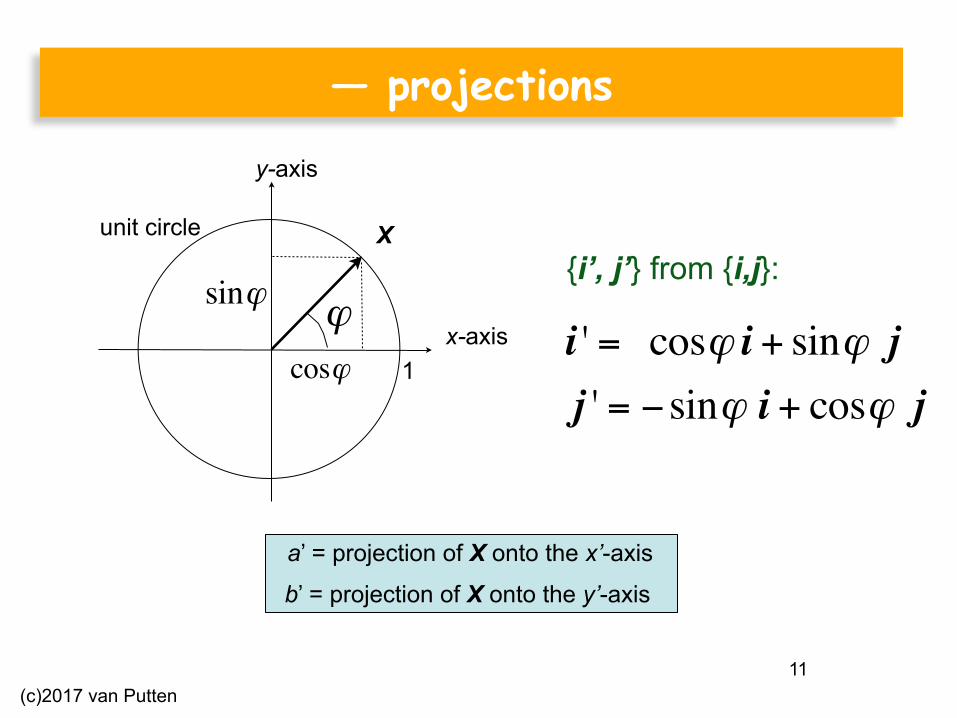
— projections

{i’, j’} from {i,j}:

a’ = projection of X onto the x’-axis

b’ = projection of X onto the y’-axis

x-axis

y-axis

Xunit circle

1

sinϕ

cosϕ

ϕi ' = cosϕ i + sinϕ jj ' = −sinϕ i + cosϕ j


Rotation: a linear transformation

A = a 'i '+ b ' j '= a '(cosϕ i + sinϕ j) + b'(−sinϕ i + cosϕ j)= (a 'cosϕ − b 'sinϕ )i +(a'sinϕ + b 'cosϕ ) j≡ ai +bj

ab

⎛

⎝⎜⎞

⎠⎟= R a '

b '⎛

⎝⎜⎞

⎠⎟=

cosϕ −sinϕsinϕ cosϕ

⎛

⎝⎜

⎞

⎠⎟

a 'b '

⎛

⎝⎜⎞

⎠⎟

R = rotation matrix


— example (I)

ϕ =ωt

ab

⎛

⎝⎜⎞

⎠⎟=

cosωt −sinωtsinωt cosωt

⎛

⎝⎜⎞

⎠⎟a 'b '

⎛

⎝⎜⎞

⎠⎟

In a co-rotating frame of the moon:

ω =2πP

angular velocity of circular motion with period P

Earth

Moon

a 'b '

⎛

⎝⎜⎞

⎠⎟= R

0⎛

⎝⎜⎞

⎠⎟


:

— example (II)ab

⎛

⎝⎜⎞

⎠⎟= R cosωt −sinωt

sinωt cosωt⎛

⎝⎜⎞

⎠⎟10

⎛

⎝⎜⎞

⎠⎟

= R cosωtsinωt

⎛

⎝⎜⎞

⎠⎟ Earth

Moon

A = ab

⎛

⎝⎜⎞

⎠⎟,

dAdt

= da / dtdb / dt

⎛

⎝⎜⎞

⎠⎟= Rω −sinωt

cosωt⎛

⎝⎜⎞

⎠⎟

Earth

Moon

A

dA/dtvelocity vector

position vector

dAdt

=dadt

⎛⎝⎜

⎞⎠⎟

2

+dbdt

⎛⎝⎜

⎞⎠⎟

2

= Rω


||A||=R d||A||/dt=0

:

15

ddti ' =ω j '

ddtj ' = −ω i '

⎧

⎨⎪⎪

⎩⎪⎪

— example (III)

{i '(t), j '(t)}Same applied to the rotating ONB

i’(t)

i’(t+dt) di’j’(t)

j’(t+dt)

dj’

(c)2017 van Putten

dϕdt

=ω

16

Trajectories in Newton’s gravitational field

Bound orbits

Unbound trajectories

(c)2017 van Putten

17

Trajectories in Newtonian gravity

Bound: elliptical orbits

Unbound: hyperbolic orbitsfocal points at ± p

ϕ

m

M

−ϕ0 <ϕ(t) <ϕ0

p-p

M

ml1 l2l1 + l2 = const.

(c)2017 van Putten

18

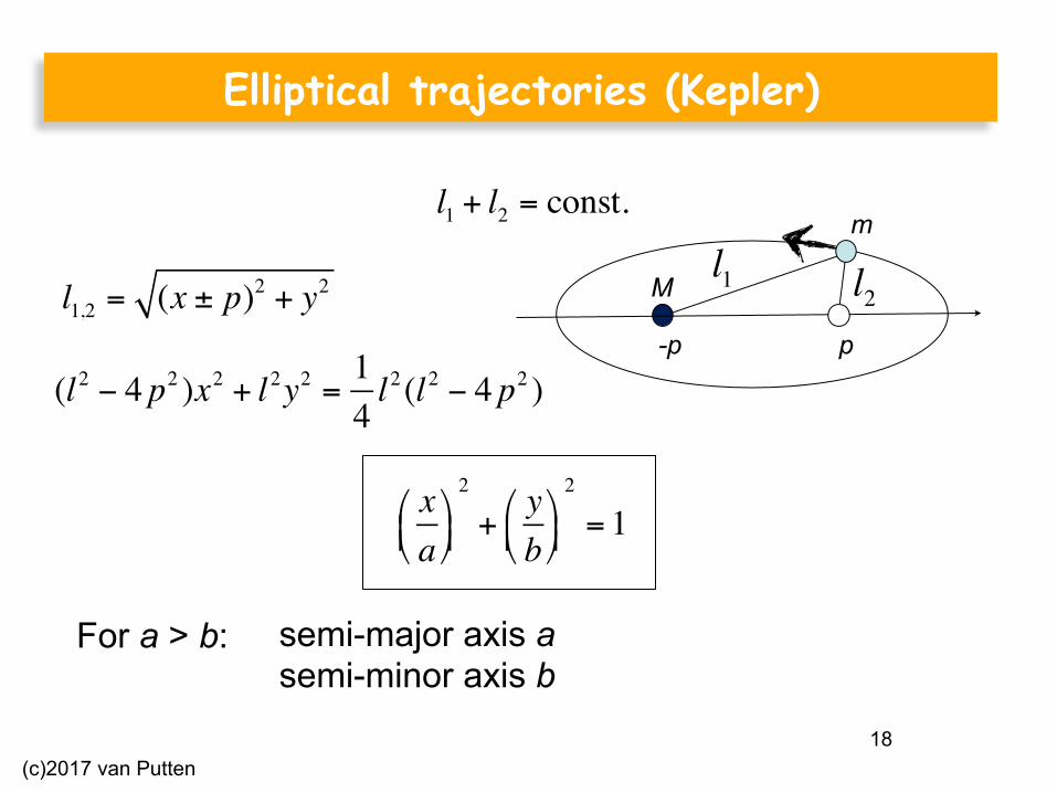
Elliptical trajectories (Kepler)

p-p

M

ml1 l2

l1 + l2 = const.

l1,2 = (x ± p)2 + y2

(l2 − 4 p2 )x2 + l2y2 = 14l2 (l2 − 4 p2 )

xa

⎛⎝⎜

⎞⎠⎟

2

+yb⎛⎝⎜

⎞⎠⎟

2

= 1

semi-major axis a semi-minor axis b

For a > b:

(c)2017 van Putten

Hyperbolic trajectories (“scattering”)

ϕ

m

M

−ϕ0 <ϕ(t) <ϕ0

r = rcosϕsinϕ

⎛

⎝⎜

⎞

⎠⎟ , r = r ϕ( )Polar coordinates:

Newton’s gravitational force F = −GMmr2

r̂, r̂ = rr,

Can show: r = const.sinϕ0 + sinϕ


20

Open and closed according to total energy H

Bound orbits:

Unbound trajectories:

closed

open (reach out to infinity)

H < 0

H > 0

(c)2017 van Putten

21

Kinetic and potential energy

Kinetic energy:

Potential energy (Newtonian gravitational binding energy):

Ek =12mv2

U = −GMmr

v

r

Ek ∝ v2 ≥ 0

U ∝−Mmr

≤ 0

(c)2017 van Putten

22

Total energy H

Total energy H: kinetic energy plus potential energy

H = Ek +U =12mv2 − GMm

r

(c)2017 van Putten

23

One-dimensional “orbits”

v = drdt

m dvdt= F = − d

drU = −

GMmr2

M m

linear motion in one dimension

dHdt

= mv dvdt+GMmr2

drdt= v m dv

dt+GMmr2

⎛⎝⎜

⎞⎠⎟= 0

Newton’s law of gravity

Total energy H is conserved

(c)2017 van Putten

24

Classification of orbits by H

H = Ek +U =12mv2 − GMm

r

Since Ek ≥ 0,U→ 0

H < 0H > 0

bound orbits: forbidden to reach infinity

upon approaching infinity

unbound orbits: allowed to reach infinity

(c)2017 van Putten

25

“Black objects”

1793: John Michell

1795: Pierre Laplace

1915: Karl Schwarzschild (exact solution)

1967: John Wheeler’s “black hole”

1974: Stephen Hawking: black holes are grey, emitting thermal radiation

(c)2017 van Putten

26

“Black objects”

H = 0 : 12mve

2 −GMmR

= 0

ve : initial velocity at the surface (“escape velocity”)

H<0: fall back

H>0: successful escapeH=0: “trapped surface” within which H < 0

(c)2017 van Putten

🙂

27

Black holes

12mc2 − GMm

RS= 0 :

ve = cConsider the limit (velocity of light)

RS =2GMc2

R = RS Radius of a

Schwarzschild black hole

(c)2017 van Putten

28

When does Newton’s law of gravity apply?

Newton’s law of gravitational attraction to a mass M applies, provided that

a) distances >> Schwarzschild radius of M

b) accelerations >> cosmological background acceleration (defined by the velocity of light and the Hubble parameter)

Newton’s law applies very well to the solar system, except for small deviations in the orbit of Mercury (small but important!)

(c)2017 van Putten

29

Force and energy

m

(c)2017 van Putten

30

Work and potential energy

ropespring

m pull

wall

a) Fs = −Fr

Fs Fr

Newton’s third law

b)Work performed stored in spring potential energyΔEs =W

W

(c)2017 van Putten

31

Work and potential energy

ΔEs = − Fs0

Δl

∫ ds

W = Fr0

Δl

∫ ds

Newton’s third law ΔEs =W

Δl

Changes are assumed to be slow and conservative, neglecting kinetic energy in m and dissipation by friction

(c)2017 van Putten

32

— example: linear spring

Fs = −kl

k is spring constant:

length of spring

force on the spring

linear range

over-stretched, nonlinear

[k]= [F][l]

=g cms−2

cm= g s−2

Hooke’s law (1660):

(c)2017 van Putten

33

— Aside: Young’s modulus

Formulation of Hooke’s law in dimensionless strain ΔL/L

(c)2017 van Putten

34

— strain-stress correlation

Young: linear relationship between stress and strain

solid material

(c)2017 van Putten

F = Aσ

σ = E Δll

E is Young’s modulus

35

— strain-stress correlation

dimensionless strain

stress linear range

over-stretched, nonlinear

[E]= [F / A][Δl / l]

= g cm−1s−2

solid material

E large: stiff material E small: soft material

(c)2017 van Putten

Dimensional analysis:

36

Hooke’s pendulum clock

u

Hooke: linear relationship between force and stretch

length l

(c)2017 van Putten

F = ku

u = l0 − l

37


u

u(t)t

F0 = mg = kl0Gravitational force balanced by a stretch of the spring:

length l

l = l0 − uΔF = F − F0 = −k(l − l0 ) = −ku

ΔF = ma = −m&&uNewton’s third law

(c)2017 van Putten

Ü

m&&u = −kuÜ

38


u

u(t)t

Time-harmonic deflection

length l

u = Acos ωt +ϕ0( ),

Equation of motion

is a 2nd order ordinary differential equation:

Two integration constants: amplitude A, initial phase ϕ0

ω =km,

P = 2πω

= 2π mk

(c)2017 van Putten

m&&u = −kuÜ

39

The free falling apple

(c)2017 van Putten

40

— trajectory in space and time

height u(t)

Free fall initial value problem

velocity du(t)/dt

time tT

fall (drop) =

area A(t)

area A(t)

(c)2017 van Putten

m&&u = −mgu(0) = H&u(0) = 0

⎧

⎨⎪

⎩⎪

Ü

ů(0)ů(0)

mů(t)=-mg

41

— free fall time

Integrate:

Integrate a second time:

u(t)− u(0) = − 12gt 2 : u(t) = H −

12gt 2

u(T ) = 0 : T =2HgFree fall time:

(A(t) = ½ g t2) u(t) = H – A

(c)2017 van Putten

&u(t)− &u(0) = −gt : &u(t) = −gtů(t) - ů(0) ů(t)

(“H - area”)

ů(t)

(c)2015 van Putten

http://www.wired.com/2014/04/basketball-physics/

The jumper


29

m&&u = −mgu(0) = 0&u(0) =V

⎧

⎨⎪

⎩⎪

43

— trajectory in space and time

The jumper “flies” according to the initial value problem

with prescribed initial height and velocity

velocity du(t)/dt

T

area A(t)

height u(t)

time tjump height area A(t)

(c)2017 van Putten

ů(0) ů(0) mů(t)=-mg

44

— total flight time

Integrate once

&u(t)− &u(0) = −gt : &u(t) =V − gtIntegrate a second time

u(t)− u(0) =Vt − 12gt 2 : u(t) =Vt − 1

2gt 2

u(T ) = 0 : T =2VgTotal flight time

&u(t*) = 0 : t* =

Vg

Time at maximal height

(c)2017 van Putten

ů(t) - ů(0) ů(t)

ů(t)

ů(t)

45

— jump height

u(t) =Vt − 12gt 2 =VT y τ( ), y τ( ) = τ 1−τ( )

Parabolic trajectory

τ =tT

expressed in dimensionless time

For parabolic curves: max y τ( ) = 14

τ =12

⎛⎝⎜

⎞⎠⎟

Maximal height reached:14VT =

V 2

2g

(c)2017 van Putten

=Ekmg

46

— duration of flying high

y(τ ) = 18 y = τ (1−τ ) = 1

4− τ −

12

⎛⎝⎜

⎞⎠⎟

2

18= τ −

12

⎛⎝⎜

⎞⎠⎟

2

: τ ± =12±

12 2

Solve

t+ − t−T

= τ + −τ− =12≅ 0.71

Relative time of flight above one-half the maximum height is

1/4

1/8

u(t)

t

H

H/2

y(τ )

τ

(c)2017 van Putten

47

Aside: Kepler orbits

(c)2017 van Putten

— polar coordinates

The trajectory of A is an ellipse: r + s = c (c is some constant)

-p px-axis

oϕ γ

A

r sr sinϕ = ssinγr cosϕ = 2p + l cosγ⎧⎨⎩

r2 = s2 + 4 pscosγ + 4 p2

scosγ = r cosϕ − 2ps = c − r

⎧

⎨⎪

⎩⎪

Write out

r(ϕ ) =

12c − 2p

2

c

1− 2p2

ccosϕ


r(ϕ ) = a 1− e2

1− ecosϕ

— ellipticity

-p px-axiso a

A1 : 2(a + p)− 2p = c

A2 : 2 p2 + b2 = c

A1

A2

p ≡ ea

b a = p2 + b2 , c = 2a

Ellipticity e:

p2 + b2

(c)2017 van Putten

In Newton’s theory, u=1/r is harmonic in phi, unifying elliptic and hyperbolic orbits.

49

Documents

Elements of classical mechanics - mvputten.org · I. Trajectories Cartesian and polar ... II. Hyperbolic and elliptic trajectories III. Three classical mechanics ... A onto the x-axis